processes

Article

The Effect of Fines on Hydraulic Conductivity ofLawrencepur, Chenab and Ravi Sand

Tanveer Ahmed Khan 1,* , Khalid Farooq 2, Mirza Muhammad 3, Mudasser Muneer Khan 1,Syyed Adnan Raheel Shah 4,*, Muhammad Shoaib 5, Muhammad Asif Aslam 1 andSyed Safdar Raza 1

1 University College of Engineering & Technology, Bahauddin Zakariya University, Multan 60000, Pakistan;mudasserkhan@bzu.edu.pk (M.M.K.); masifaslam@bzu.edu.pk (M.A.A.); safdarshah91@yahoo.com (S.S.R.)

2 Department of Civil Engineering, University of Engineering & Technology, Lahore 54700, Pakistan;kfch@uet.edu.pk

3 National Engineering Services (NESPAK), Lahore 54700, Pakistan; mirza_muhammad@yahoo.com4 Department of Civil Engineering, Pakistan Institute of Engineering and Technology, Multan 60000, Pakistan5 Department of Agricultural Engineering, Bahauddin Zakariya University, Multan 60000, Pakistan;

muhammadshoaib@bzu.edu.pk* Correspondence: tanveerkhan@bzu.edu.pk (T.A.K.); syyed.adnanraheelshah@uhasselt.be (S.A.R.S.);

Tel.: +92-333-880-4950 (T.A.K.)

Received: 6 July 2019; Accepted: 12 October 2019; Published: 2 November 2019�����������������

Abstract: The amount of fines in sand greatly influence the permeability of sandy soils. Thus, thisresearch was conducted to study the effect of plastic and non-plastic fines on the permeability ofthree types of sands (Lawrencepur sand, Chenab sand and Ravi sand). For this purpose, plastic andnon-plastic fines were collected from different location of Lahore. Samples were prepared by mixingplastic and non-plastic fines into each type of sand separately, in amounts ranging from 0% to 50%with increments of five percent. Overall 63 samples were prepared. Sieve analysis and hydrometricanalysis were performed to obtain particle size distribution for each sample. Atterberg’s limits werealso determined and each sample was classified according to the Unified Soil Classification System(USCS). Compaction tests were performed on all samples as per the procedure in a standard Proctortest. The test samples were compacted in permeability molds with optimum moisture contents toobtain the density, as per a standard Proctor test. Hydraulic conductivity tests were performed on allsixty-three samples using a constant head permeameter and a falling head permeameter. Permeabilityresults were plotted against the percentage of fines added. It was noted from the curves that thepermeability of sand-fine mixtures shows a decreasing trend with the addition of fine contents. A fewtrials were performed to formulate a correlation. Validation of the correlation was performed withthe results of 52 data sets from the field. Finally, the devised correlation was compared with threeempirical equations proposed by Mujtaba, Kozeny–Carman and Hazen.

Keywords: fluid; soil; permeability; sand; fines; transport

1. Introduction

Permeability is an important physical property of soil whose understanding is essential insettlement, seepage and stability analyses [1,2]. The stability of structures depends to a large degree onthe interaction of the said soil with water, or in other words, the ability of water to flow through thesoil [3,4]. Moreover, in-depth understanding of soil permeability is needed to estimate the quantityof seepage under and through dams, levees and embankments etc. It also helps to plan dewateringmethods to facilitate underground construction [5]. Furthermore, many dam failures have occurreddue to insufficient geotechnical and geological investigations. The failure due to seepage through adam body and/or foundation accounts for almost 30% of total failures [6].

Processes 2019, 7, 796; doi:10.3390/pr7110796 www.mdpi.com/journal/processes

Processes 2019, 7, 796 2 of 13

While studying the soil properties, D represents the diameter of particles, and D50 means acumulative 50% point of diameter (or 50% pass particle size); D10 means a cumulative 10% point ofdiameter. Numerous relationships between the permeability and grain size distribution indices (likeuniformity coefficient, coefficient of gradation, median grain size (D50) and effective grain size (D10))of the soil have been reported, such as those in Hazen [7], Zunker [8], Carman [9], Burmister [10],Michaels and Lin [11], Olsen [12], Mitchell et al. [13] and Wang and Huang [14]. Lately, Alyamani andSen [15], Koltermann and Gorelick [16], D’Andrea and Boadu [17], Chapuis [18], Sinha and Wang [19]and Cote et al. [20] established different models to corelate the hydraulic conductivity of soils with theirindex properties. The hydraulic conductivity has been discussed with sand as well [21], focusing ongrain size of soils [22]. However, equations based on grain size distribution do not yield good resultsfor clayey soils and soils with effective grain sizes greater than 3 mm [23]. The presence of grains ofextreme-size also produces inaccurate predictions of soil permeability. The prediction of permeabilityof well-graded soils is particularly difficult due to the void-filling trend of various-sized particles [24].On the other hand, laboratory and field tests have their limitations and weaknesses, such as thevariation of permeability in horizontal and vertical directions in soils [25]; disturbances in extractedsamples and how closely they represent field conditions [26,27]; and costly and time-consuming fieldpumping tests [27].

Silica fume was used to improve the qualities of clay used as clay liners. It was observed that itreduced the plasticity index (from CH to CL), permeability and swelling pressure considerably andincreased the compressive strength [28]. Two types of silts, fine sands and coarse sands were mixedwith varying amounts of commercial bentonite, and hydraulic conductivity was determined with aconsolidometer permeameter. It was found that when bentonite was mixed with coarser material, thehydraulic conductivity (log) changed linearly with void ratio [1]. The permeability of dune sand wasgreatly affected and reduced to 10−8 cm/s from 10−4 cm/s with the addition of 10% bentonite [29].

Shear strength and permeability are two important characteristics desirable for almost allgeotechnical projects. In many cases, these two are required concurrently, meaning these should beattained at maximum dry density (MDD) and optimum moisture content (OMC) of soil. As laboratorytests for determining permeability and shear strength are time-consuming, it is desirable to devisemodels to predict compacted soil’s permeability based on the index properties of soils. Efforts havebeen made to relate these important parameters with the indices of soils, such as grain size distributionand plasticity characteristics [5].

Pakistan is a vast country having large plains. Rivers (Indus, Chenab, Jhelum, Ravi, Bias and Sutlej)along with other tributaries pass through these plains. Sands of different gradations are encounteredin these rivers and are widely used in construction works. The areas near the rivers are regularlysubjected to the erosive action of river flow, especially during flood seasons, also causing damageto the river training works along the rivers and other infrastructure. In most cases, a need arises tomodify the properties of riverbed materials by mixing these with other, locally available, cheapermaterials. In this context, the predicted permeability (hydraulic conductivity) values of these sandsmixed with different proportions of fines will be very helpful. Thus, in this research sand samples fromChenab, Lawrencepur and Ravi rivers were used. The two fines (plastic and non-plastic) were addedto each type of the sand separately to prepare representative samples on MDD and OMC determinedthrough the standard Proctor test, and permeability tests were executed. The results were analyzed,and a correlation was developed to predict permeability values from the given parameters. Finally, thecorrelation developed was compared with three other permeability correlations.

2. Materials and Methods

Three types of sands (quartz as main mineral) were collected from Chenab, Lawrencepur andRavi rivers. These are the main and the most common type of fine aggregates used in various civilengineering projects in Pakistan [30]. Plastic and non-plastic fines are predominantly clays and siltsrespectively, and were collected from different localities of Lahore, Pakistan. Chenab, Lawrencepur

Processes 2019, 7, 796 3 of 13

and Ravi sands are designated as CS, LS and RS respectively, in the following discussion. Furthermore,PF represents plastic fines and NPF represents non-plastic fines. PF were collected from near ExpoCentre Lahore, whereas NPF from the Habanspura area of Lahore.

All sands and fine samples were separated from vegetation, clods and other materials of largersizes. Larger sizes in PF and NPF were broken into small fractions. All materials were then passedthrough sieve number 4. Each PF and NPF were added separately to each type of sand, ranging from0% to 50% of the total weight of sample. Overall 63 samples were prepared and following tests wereperformed in the laboratory:

(a) Grain size analysis (ASTM D-422);(b) Standard Proctor test (ASTM D-422);(c) Atterberg limits (ASTM D-4318);(d) Constant head permeability test (ASTM-D 2434);(e) Falling head permeability test.

3. Results and Discussion

3.1. Grain Size Analysis

The gradation curves of CS, LS and RS are given in Figure 1, along with curves of NPF and PF. TheLS was well graded when compared to CS and RS, whereas RS was the most uniformly graded and CSlies somewhere between the two. Understandably, the curve of PF is on the finer side of the curveof NPF. Gradation curves were drawn for all 63 samples and observations were made to calculatethe uniformity coefficient (Cu) and coefficient of gradation (Cc). Consistency limits (liquid limit andplastic limit) were determined for the soil samples attaining some plasticity due to the addition of fines.All samples were then classified according to Unified Soil Classification System (USCS). The mediangrain size (D50, diameter corresponding to 50% finer) varied between 0.01 and 0.9 mm, whereas theeffective grain size (D10) varied from 0.005 to 0.33 mm. The gradation of all samples is not shown heredue to a very large number of curves, though the observations from the gradation curves, consistencylimits and soil symbols of all the samples are listed in Table 1.

Most samples were non-plastic (NP) except some with higher percentages of plastic fines. It isalso noted that most of the samples were silty sand (SM). As per USCS, both LS and CS were poorlygraded sand (SP) while RS was poorly graded sand with silt (SP-SM).

Processes 2019, 7, x FOR PEER REVIEW 3 of 13

engineering projects in Pakistan [30]. Plastic and non-plastic fines are predominantly clays and silts respectively, and were collected from different localities of Lahore, Pakistan. Chenab, Lawrencepur and Ravi sands are designated as CS, LS and RS respectively, in the following discussion. Furthermore, PF represents plastic fines and NPF represents non-plastic fines. PF were collected from near Expo Centre Lahore, whereas NPF from the Habanspura area of Lahore.

All sands and fine samples were separated from vegetation, clods and other materials of larger sizes. Larger sizes in PF and NPF were broken into small fractions. All materials were then passed through sieve number 4. Each PF and NPF were added separately to each type of sand, ranging from 0% to 50% of the total weight of sample. Overall 63 samples were prepared and following tests were performed in the laboratory:

(a) Grain size analysis (ASTM D-422); (b) Standard Proctor test (ASTM D-422); (c) Atterberg limits (ASTM D-4318); (d) Constant head permeability test (ASTM-D 2434); (e) Falling head permeability test.

3. Results and Discussion

3.1. Grain Size Analysis

The gradation curves of CS, LS and RS are given in Figure 1, along with curves of NPF and PF. The LS was well graded when compared to CS and RS, whereas RS was the most uniformly graded and CS lies somewhere between the two. Understandably, the curve of PF is on the finer side of the curve of NPF. Gradation curves were drawn for all 63 samples and observations were made to calculate the uniformity coefficient (Cu) and coefficient of gradation (Cc). Consistency limits (liquid limit and plastic limit) were determined for the soil samples attaining some plasticity due to the addition of fines. All samples were then classified according to Unified Soil Classification System (USCS). The median grain size (D50, diameter corresponding to 50% finer) varied between 0.01 and 0.9 mm, whereas the effective grain size (D10) varied from 0.005 to 0.33 mm. The gradation of all samples is not shown here due to a very large number of curves, though the observations from the gradation curves, consistency limits and soil symbols of all the samples are listed in Table 1.

Most samples were non-plastic (NP) except some with higher percentages of plastic fines. It is also noted that most of the samples were silty sand (SM). As per USCS, both LS and CS were poorly graded sand (SP) while RS was poorly graded sand with silt (SP-SM).

Figure 1. The gradation curves of three types of sands and two fines.

0.0010.010.11100

10

20

30

40

50

60

70

80

90

100

% F

iner

Grain Size (mm)- log scale

LS CS RS NPF PF

Figure 1. The gradation curves of three types of sands and two fines.

Processes 2019, 7, 796 4 of 13

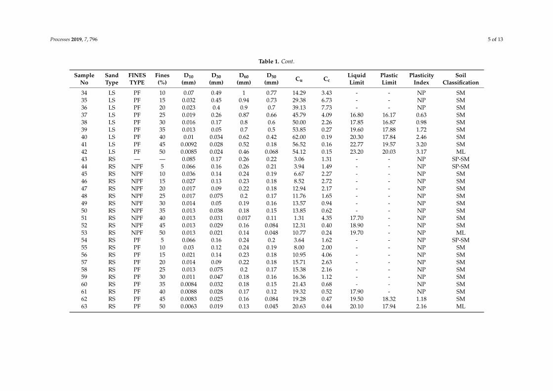
Table 1. Data from gradation curves, consistency limits and soil symbols of all the samples.

SampleNo

SandType

FINESTYPE

Fines(%)

D10(mm)

D30(mm)

D60(mm)

D50(mm) Cu Cc

LiquidLimit

PlasticLimit

PlasticityIndex

SoilClassification

1 CS — — 0.09 0.16 0.31 0.25 3.44 0.92 - - NP SP2 CS NPF 5 0.076 0.16 0.28 0.25 3.68 1.20 - - NP SP-SM3 CS NPF 10 0.055 0.15 0.28 0.23 5.09 1.46 - - NP SM4 CS NPF 15 0.043 0.13 0.27 0.21 6.28 1.46 - - NP SM5 CS NPF 20 0.025 0.098 0.22 0.16 8.80 1.75 - - NP SM6 CS NPF 25 0.026 0.081 0.23 0.18 8.85 1.10 - - NP SM7 CS NPF 30 0.024 0.067 0.22 0.17 9.17 0.85 - - NP SM8 CS NPF 35 0.016 0.05 0.19 0.14 11.88 0.82 - - NP SM9 CS NPF 40 0.015 0.042 0.18 0.12 12.00 0.65 16.85 - NP SM

10 CS NPF 45 0.013 0.033 0.17 0.077 13.08 0.49 18.25 - NP SM11 CS NPF 50 0.013 0.028 0.14 0.067 10.77 0.43 19.30 - NP ML12 CS PF 5 0.053 0.16 0.28 0.24 5.28 1.73 - - NP SP-SM13 CS PF 10 0.051 0.14 0.28 0.22 5.49 1.37 - - NP SM14 CS PF 15 0.03 0.13 0.26 0.22 8.67 2.17 - - NP SM15 CS PF 20 0.018 0.098 0.26 0.18 14.44 2.05 - - NP SM16 CS PF 25 0.017 0.077 0.23 0.17 13.53 1.52 - - NP SM17 CS PF 30 0.013 0.055 0.22 0.17 16.92 1.06 - - NP SM18 CS PF 35 0.012 0.039 0.19 0.14 15.83 0.67 - - NP SM19 CS PF 40 0.0094 0.03 0.18 0.13 19.15 0.53 18.80 - NP SM20 CS PF 45 0.0085 0.027 0.17 0.087 20.00 0.50 19.75 18.14 1.61 SM21 CS PF 50 0.0078 0.023 0.14 0.058 17.95 0.48 20.25 17.97 2.28 ML22 LS — — 0.26 0.57 1.2 0.87 4.62 1.04 - - NP SP23 LS NPF 5 0.17 0.54 1.1 0.86 6.47 1.56 - - NP SP-SM24 LS NPF 10 0.06 0.49 1 0.78 16.67 4.00 - - NP SM25 LS NPF 15 0.046 0.45 0.94 0.74 20.43 4.68 - - NP SM26 LS NPF 20 0.039 0.41 0.9 0.7 23.08 4.79 - - NP SM27 LS NPF 25 0.029 0.26 0.87 0.67 30.00 2.68 - - NP SM28 LS NPF 30 0.026 0.17 0.8 0.6 30.77 1.39 14.30 - NP SM29 LS NPF 35 0.016 0.066 0.7 0.51 43.75 0.39 15.40 - NP SM30 LS NPF 40 0.015 0.041 0.6 0.41 40.00 0.19 16.70 - NP SM31 LS NPF 45 0.014 0.028 0.51 0.17 36.43 0.11 18.72 - NP SM32 LS NPF 50 0.013 0.028 0.45 0.07 34.62 0.13 19.80 - NP ML33 LS PF 5 0.18 0.55 1.1 0.84 6.11 1.53 - - NP SP-SM

Processes 2019, 7, 796 5 of 13

Table 1. Cont.

SampleNo

SandType

FINESTYPE

Fines(%)

D10(mm)

D30(mm)

D60(mm)

D50(mm) Cu Cc

LiquidLimit

PlasticLimit

PlasticityIndex

SoilClassification

34 LS PF 10 0.07 0.49 1 0.77 14.29 3.43 - - NP SM35 LS PF 15 0.032 0.45 0.94 0.73 29.38 6.73 - - NP SM36 LS PF 20 0.023 0.4 0.9 0.7 39.13 7.73 - - NP SM37 LS PF 25 0.019 0.26 0.87 0.66 45.79 4.09 16.80 16.17 0.63 SM38 LS PF 30 0.016 0.17 0.8 0.6 50.00 2.26 17.85 16.87 0.98 SM39 LS PF 35 0.013 0.05 0.7 0.5 53.85 0.27 19.60 17.88 1.72 SM40 LS PF 40 0.01 0.034 0.62 0.42 62.00 0.19 20.30 17.84 2.46 SM41 LS PF 45 0.0092 0.028 0.52 0.18 56.52 0.16 22.77 19.57 3.20 SM42 LS PF 50 0.0085 0.024 0.46 0.068 54.12 0.15 23.20 20.03 3.17 ML43 RS — — 0.085 0.17 0.26 0.22 3.06 1.31 - - NP SP-SM44 RS NPF 5 0.066 0.16 0.26 0.21 3.94 1.49 - - NP SP-SM45 RS NPF 10 0.036 0.14 0.24 0.19 6.67 2.27 - - NP SM46 RS NPF 15 0.027 0.13 0.23 0.18 8.52 2.72 - - NP SM47 RS NPF 20 0.017 0.09 0.22 0.18 12.94 2.17 - - NP SM48 RS NPF 25 0.017 0.075 0.2 0.17 11.76 1.65 - - NP SM49 RS NPF 30 0.014 0.05 0.19 0.16 13.57 0.94 - - NP SM50 RS NPF 35 0.013 0.038 0.18 0.15 13.85 0.62 - - NP SM51 RS NPF 40 0.013 0.031 0.017 0.11 1.31 4.35 17.70 - NP SM52 RS NPF 45 0.013 0.029 0.16 0.084 12.31 0.40 18.90 - NP SM53 RS NPF 50 0.013 0.021 0.14 0.048 10.77 0.24 19.70 - NP ML54 RS PF 5 0.066 0.16 0.24 0.2 3.64 1.62 - - NP SP-SM55 RS PF 10 0.03 0.12 0.24 0.19 8.00 2.00 - - NP SM56 RS PF 15 0.021 0.14 0.23 0.18 10.95 4.06 - - NP SM57 RS PF 20 0.014 0.09 0.22 0.18 15.71 2.63 - - NP SM58 RS PF 25 0.013 0.075 0.2 0.17 15.38 2.16 - - NP SM59 RS PF 30 0.011 0.047 0.18 0.16 16.36 1.12 - - NP SM60 RS PF 35 0.0084 0.032 0.18 0.15 21.43 0.68 - - NP SM61 RS PF 40 0.0088 0.028 0.17 0.12 19.32 0.52 17.90 - NP SM62 RS PF 45 0.0083 0.025 0.16 0.084 19.28 0.47 19.50 18.32 1.18 SM63 RS PF 50 0.0063 0.019 0.13 0.045 20.63 0.44 20.10 17.94 2.16 ML

Processes 2019, 7, 796 6 of 13

3.2. Compaction Tests

Standard Proctor tests were performed on all 63 samples in accordance with the guidelines ofASTM D-698. The lowest value of MDD (1.6 g/cm3) was observed for Ravi sand. This was obvious,as RS was the most uniformly graded soil (mentioned earlier). The highest MDD was for Lawrencepursand mixed with 20% non-plastic fines (LS20NPF). Figure 2 shows the compaction curves of the lowestdry density (RS), highest dry density (LS20NPF), CS and LS soil samples.

The variations in MDD and OMC with the addition of two fines are shown in Figures 3 and 4respectively. For LS mixed with both fines, MDD increased up to 20% fine content and then startedto decrease, whereas, for both CS and RS, MDD increased for up to 35% fine content and then eitherremained the same or decreased a small amount. The initial increase in MDD may be attributable tothe occupation of voids in sand by the fines. The decline in density after reaching the peak may be dueto the bouncing of particles, thereby increasing the space within particles and reducing dry density.

Processes 2019, 7, x FOR PEER REVIEW 6 of 13

3.2. Compaction Tests

Standard Proctor tests were performed on all 63 samples in accordance with the guidelines of ASTM D-698. The lowest value of MDD (1.6 g/cm3) was observed for Ravi sand. This was obvious, as RS was the most uniformly graded soil (mentioned earlier). The highest MDD was for Lawrencepur sand mixed with 20% non-plastic fines (LS20NPF). Figure 2 shows the compaction curves of the lowest dry density (RS), highest dry density (LS20NPF), CS and LS soil samples.

The variations in MDD and OMC with the addition of two fines are shown in Figures 3 and 4 respectively. For LS mixed with both fines, MDD increased up to 20% fine content and then started to decrease, whereas, for both CS and RS, MDD increased for up to 35% fine content and then either remained the same or decreased a small amount. The initial increase in MDD may be attributable to the occupation of voids in sand by the fines. The decline in density after reaching the peak may be due to the bouncing of particles, thereby increasing the space within particles and reducing dry density.

Figure 2. Standard Proctor test results.

Figure 3. Variation in maximum dry density with different fine contents.

4 6 8 10 12 14 16 18 20 22

1.5

1.6

1.7

1.8

1.9

2.0

2.1

2.2

Dry

Des

nity

(g/c

m3 )

Moisture Content %

LS LS20NPF CS RS

0 10 20 30 40 50

1.6

1.7

1.8

1.9

2.0

2.1

2.2

Max

. Dry

Den

sity

(gm

/cm

3 )

Fine Content (%)

LS with NPF LS with PF CS with NPF CS with PF RS with NPF RS with PF

Figure 2. Standard Proctor test results.

Processes 2019, 7, x FOR PEER REVIEW 6 of 13

3.2. Compaction Tests

Standard Proctor tests were performed on all 63 samples in accordance with the guidelines of ASTM D-698. The lowest value of MDD (1.6 g/cm3) was observed for Ravi sand. This was obvious, as RS was the most uniformly graded soil (mentioned earlier). The highest MDD was for Lawrencepur sand mixed with 20% non-plastic fines (LS20NPF). Figure 2 shows the compaction curves of the lowest dry density (RS), highest dry density (LS20NPF), CS and LS soil samples.

The variations in MDD and OMC with the addition of two fines are shown in Figures 3 and 4 respectively. For LS mixed with both fines, MDD increased up to 20% fine content and then started to decrease, whereas, for both CS and RS, MDD increased for up to 35% fine content and then either remained the same or decreased a small amount. The initial increase in MDD may be attributable to the occupation of voids in sand by the fines. The decline in density after reaching the peak may be due to the bouncing of particles, thereby increasing the space within particles and reducing dry density.

Figure 2. Standard Proctor test results.

Figure 3. Variation in maximum dry density with different fine contents.

4 6 8 10 12 14 16 18 20 22

1.5

1.6

1.7

1.8

1.9

2.0

2.1

2.2

Dry

Des

nity

(g/c

m3 )

Moisture Content %

LS LS20NPF CS RS

0 10 20 30 40 50

1.6

1.7

1.8

1.9

2.0

2.1

2.2

Max

. Dry

Den

sity

(gm

/cm

3 )

Fine Content (%)

LS with NPF LS with PF CS with NPF CS with PF RS with NPF RS with PF

Figure 3. Variation in maximum dry density with different fine contents.

Processes 2019, 7, 796 7 of 13Processes 2019, 7, x FOR PEER REVIEW 7 of 13

Figure 4. Variation in optimum moisture content with different fine contents.

3.3. Permeability

Constant head permeability tests were performed in accordance with the guidelines of ASTM D-2434 on LS mixed with up to 25% and 20% of NPF and PF respectively. The same test was conducted on CS and RS mixed with both fines up to 20%. Falling head permeability tests were performed on all remaining samples. The results of the tests are shown in Figure 5. The figure shows that the permeability of all three types of sands decreases with increasing fine contents. The rate of decrease in permeability is very weighty up until 20% fine content and then reduces significantly. Amongst the nonamended sands, LS had a maximum permeability value of 4.63 × 10−3 cm/sec, whereas for CS and RS, the observed values were 2.14 × 10−3 cm/sec and 1.98 × 10−3 cm/sec respectively. These values seem to be related with their median grain size (D50). D50s for CS, LS and RS were 0.25, 0.87 and 0.22 mm respectively. In amended soils, the minimum permeability of 6.39 × 10−6 cm/sec was noted for RS mixed with 50% PF.

Figure 5. Variation in permeability with different fine contents.

0 10 20 30 40 50

15.5

16.0

16.5

17.0

17.5

18.0

18.5

Opt

imum

Moi

stur

e C

onte

nt (%

)

Fine Content (%)

LS with NPF LS with PF CS with NPF CS with PF RS with NPF RS with PF

0 10 20 30 40 500.0

1.0x10-3

2.0x10-3

3.0x10-3

4.0x10-3

5.0x10-3

Perm

eabi

lity

(cm

/sec

)

Fine Content (%)

LS with NPF LS with PF CS with NPF CS with PF RS with NPF RS with PF

Figure 4. Variation in optimum moisture content with different fine contents.

3.3. Permeability

Constant head permeability tests were performed in accordance with the guidelines of ASTMD-2434 on LS mixed with up to 25% and 20% of NPF and PF respectively. The same test was conductedon CS and RS mixed with both fines up to 20%. Falling head permeability tests were performedon all remaining samples. The results of the tests are shown in Figure 5. The figure shows that thepermeability of all three types of sands decreases with increasing fine contents. The rate of decreasein permeability is very weighty up until 20% fine content and then reduces significantly. Amongstthe nonamended sands, LS had a maximum permeability value of 4.63 × 10−3 cm/sec, whereas forCS and RS, the observed values were 2.14 × 10−3 cm/sec and 1.98 × 10−3 cm/sec respectively. Thesevalues seem to be related with their median grain size (D50). D50s for CS, LS and RS were 0.25, 0.87and 0.22 mm respectively. In amended soils, the minimum permeability of 6.39 × 10−6 cm/sec wasnoted for RS mixed with 50% PF.

Processes 2019, 7, x FOR PEER REVIEW 7 of 13

Figure 4. Variation in optimum moisture content with different fine contents.

3.3. Permeability

Constant head permeability tests were performed in accordance with the guidelines of ASTM D-2434 on LS mixed with up to 25% and 20% of NPF and PF respectively. The same test was conducted on CS and RS mixed with both fines up to 20%. Falling head permeability tests were performed on all remaining samples. The results of the tests are shown in Figure 5. The figure shows that the permeability of all three types of sands decreases with increasing fine contents. The rate of decrease in permeability is very weighty up until 20% fine content and then reduces significantly. Amongst the nonamended sands, LS had a maximum permeability value of 4.63 × 10−3 cm/sec, whereas for CS and RS, the observed values were 2.14 × 10−3 cm/sec and 1.98 × 10−3 cm/sec respectively. These values seem to be related with their median grain size (D50). D50s for CS, LS and RS were 0.25, 0.87 and 0.22 mm respectively. In amended soils, the minimum permeability of 6.39 × 10−6 cm/sec was noted for RS mixed with 50% PF.

Figure 5. Variation in permeability with different fine contents.

0 10 20 30 40 50

15.5

16.0

16.5

17.0

17.5

18.0

18.5

Opt

imum

Moi

stur

e C

onte

nt (%

)

Fine Content (%)

LS with NPF LS with PF CS with NPF CS with PF RS with NPF RS with PF

0 10 20 30 40 500.0

1.0x10-3

2.0x10-3

3.0x10-3

4.0x10-3

5.0x10-3

Perm

eabi

lity

(cm

/sec

)

Fine Content (%)

LS with NPF LS with PF CS with NPF CS with PF RS with NPF RS with PF

Figure 5. Variation in permeability with different fine contents.

Processes 2019, 7, 796 8 of 13

3.4. The Development of Correlations

Analyses were performed with the set of ρd (dry density), D10, D30, D50, D60, Cu, and Cc valuesto select the most suitable independent variables to develop correlations as D60 defines 60 % of thesoil particles are finer than this size, D30 defines 30% of the particles are finer than this size and D10defines 10% of the particles are finer than this size. The results of the analysis of ρd, D10 and D50 onpermeability are shown in Figures 6–8 respectively. The trend for permeability versus ρd is a decreasingone, though the data is somewhat scattered. For both D10 and D50, the permeability increases with anincrease in particle size.

Processes 2019, 7, x FOR PEER REVIEW 8 of 13

3.4. The Development of Correlations

Analyses were performed with the set of ρd (dry density), D10, D30, D50, D60, Cu, and Cc values to select the most suitable independent variables to develop correlations as D60 defines 60 % of the soil particles are finer than this size, D30 defines 30% of the particles are finer than this size and D10 defines 10% of the particles are finer than this size. The results of the analysis of ρd, D10 and D50 on permeability are shown in Figures 6–8 respectively. The trend for permeability versus ρd is a decreasing one, though the data is somewhat scattered. For both D10 and D50, the permeability increases with an increase in particle size.

Figure 6. Permeability versus maximum dry density.

Figure 7. Permeability versus D10.

1.5 1.6 1.7 1.8 1.9 2.0 2.1 2.20.0

5.0x10-4

1.0x10-3

1.5x10-3

2.0x10-3

2.5x10-3

Perm

eabi

lity

(cm

/sec

)

MDD (gm/cm3)

0.000 0.025 0.050 0.075 0.1000.0

5.0x10-4

1.0x10-3

1.5x10-3

2.0x10-3

2.5x10-3

3.0x10-3

Perm

eabi

lity

(cm

/sec

)

D10 (mm)

Figure 6. Permeability versus maximum dry density.

Processes 2019, 7, x FOR PEER REVIEW 8 of 13

3.4. The Development of Correlations

Analyses were performed with the set of ρd (dry density), D10, D30, D50, D60, Cu, and Cc values to select the most suitable independent variables to develop correlations as D60 defines 60 % of the soil particles are finer than this size, D30 defines 30% of the particles are finer than this size and D10 defines 10% of the particles are finer than this size. The results of the analysis of ρd, D10 and D50 on permeability are shown in Figures 6–8 respectively. The trend for permeability versus ρd is a decreasing one, though the data is somewhat scattered. For both D10 and D50, the permeability increases with an increase in particle size.

Figure 6. Permeability versus maximum dry density.

Figure 7. Permeability versus D10.

1.5 1.6 1.7 1.8 1.9 2.0 2.1 2.20.0

5.0x10-4

1.0x10-3

1.5x10-3

2.0x10-3

2.5x10-3

Perm

eabi

lity

(cm

/sec

)

MDD (gm/cm3)

0.000 0.025 0.050 0.075 0.1000.0

5.0x10-4

1.0x10-3

1.5x10-3

2.0x10-3

2.5x10-3

3.0x10-3

Perm

eabi

lity

(cm

/sec

)

D10 (mm)

Figure 7. Permeability versus D10.

Processes 2019, 7, 796 9 of 13Processes 2019, 7, x FOR PEER REVIEW 9 of 13

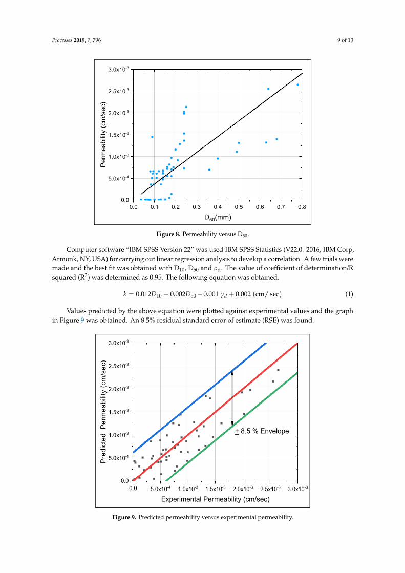
Figure 8. Permeability versus D50.

Computer software “IBM SPSS Version 22” was used IBM SPSS Statistics (V22.0. 2016, IBM Corp, Armonk, NY, USA) for carrying out linear regression analysis to develop a correlation. A few trials were made and the best fit was obtained with D10, D50 and ρd. The value of coefficient of determination/R squared (R2) was determined as 0.95. The following equation was obtained. 𝑘 = 0.012𝐷 + 0.002𝐷 − 0.001 𝛾 + 0.002 (cm/sec) (1)

Values predicted by the above equation were plotted against experimental values and the graph in Figure 9 was obtained. An 8.5% residual standard error of estimate (RSE) was found.

Figure 9. Predicted permeability versus experimental permeability.

3.5. Data Validation

0.0 0.1 0.2 0.3 0.4 0.5 0.6 0.7 0.80.0

5.0x10-4

1.0x10-3

1.5x10-3

2.0x10-3

2.5x10-3

3.0x10-3

Perm

eabi

lity

(cm

/sec

)

D50(mm)

0.0 5.0x10-4 1.0x10-3 1.5x10-3 2.0x10-3 2.5x10-3 3.0x10-30.0

5.0x10-4

1.0x10-3

1.5x10-3

2.0x10-3

2.5x10-3

3.0x10-3

Pred

icte

d P

erm

eabi

lity

(cm

/sec

)

Experimental Permeability (cm/sec)

+ 8.5 % Envelope

Figure 8. Permeability versus D50.

Computer software “IBM SPSS Version 22” was used IBM SPSS Statistics (V22.0. 2016, IBM Corp,Armonk, NY, USA) for carrying out linear regression analysis to develop a correlation. A few trials weremade and the best fit was obtained with D10, D50 and ρd. The value of coefficient of determination/Rsquared (R2) was determined as 0.95. The following equation was obtained.

k = 0.012D10 + 0.002D50 − 0.001 γd + 0.002 (cm/ sec) (1)

Values predicted by the above equation were plotted against experimental values and the graphin Figure 9 was obtained. An 8.5% residual standard error of estimate (RSE) was found.

Processes 2019, 7, x FOR PEER REVIEW 9 of 13

Figure 8. Permeability versus D50.

Computer software “IBM SPSS Version 22” was used IBM SPSS Statistics (V22.0. 2016, IBM Corp, Armonk, NY, USA) for carrying out linear regression analysis to develop a correlation. A few trials were made and the best fit was obtained with D10, D50 and ρd. The value of coefficient of determination/R squared (R2) was determined as 0.95. The following equation was obtained. 𝑘 = 0.012𝐷 + 0.002𝐷 − 0.001 𝛾 + 0.002 (cm/sec) (1)

Values predicted by the above equation were plotted against experimental values and the graph in Figure 9 was obtained. An 8.5% residual standard error of estimate (RSE) was found.

Figure 9. Predicted permeability versus experimental permeability.

3.5. Data Validation

0.0 0.1 0.2 0.3 0.4 0.5 0.6 0.7 0.80.0

5.0x10-4

1.0x10-3

1.5x10-3

2.0x10-3

2.5x10-3

3.0x10-3

Perm

eabi

lity

(cm

/sec

)

D50(mm)

0.0 5.0x10-4 1.0x10-3 1.5x10-3 2.0x10-3 2.5x10-3 3.0x10-30.0

5.0x10-4

1.0x10-3

1.5x10-3

2.0x10-3

2.5x10-3

3.0x10-3

Pred

icte

d P

erm

eabi

lity

(cm

/sec

)

Experimental Permeability (cm/sec)

+ 8.5 % Envelope

Figure 9. Predicted permeability versus experimental permeability.

Processes 2019, 7, 796 10 of 13

3.5. Data Validation

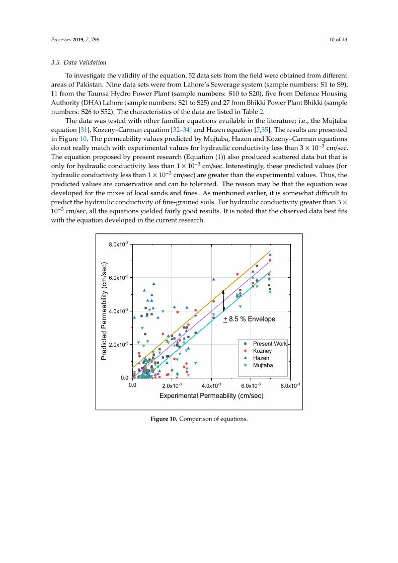
To investigate the validity of the equation, 52 data sets from the field were obtained from differentareas of Pakistan. Nine data sets were from Lahore’s Sewerage system (sample numbers: S1 to S9),11 from the Taunsa Hydro Power Plant (sample numbers: S10 to S20), five from Defence HousingAuthority (DHA) Lahore (sample numbers: S21 to S25) and 27 from Bhikki Power Plant Bhikki (samplenumbers: S26 to S52). The characteristics of the data are listed in Table 2.

The data was tested with other familiar equations available in the literature; i.e., the Mujtabaequation [31], Kozeny–Carman equation [32–34] and Hazen equation [7,35]. The results are presentedin Figure 10. The permeability values predicted by Mujtaba, Hazen and Kozeny–Carman equationsdo not really match with experimental values for hydraulic conductivity less than 3 × 10−3 cm/sec.The equation proposed by present research (Equation (1)) also produced scattered data but that isonly for hydraulic conductivity less than 1 × 10−3 cm/sec. Interestingly, these predicted values (forhydraulic conductivity less than 1 × 10−3 cm/sec) are greater than the experimental values. Thus, thepredicted values are conservative and can be tolerated. The reason may be that the equation wasdeveloped for the mixes of local sands and fines. As mentioned earlier, it is somewhat difficult topredict the hydraulic conductivity of fine-grained soils. For hydraulic conductivity greater than 3 ×10−3 cm/sec, all the equations yielded fairly good results. It is noted that the observed data best fitswith the equation developed in the current research.

Processes 2019, 7, x FOR PEER REVIEW 10 of 13

To investigate the validity of the equation, 52 data sets from the field were obtained from different areas of Pakistan. Nine data sets were from Lahore’s Sewerage system (sample numbers: S1 to S9), 11 from the Taunsa Hydro Power Plant (sample numbers: S10 to S20), five from Defence Housing Authority (DHA) Lahore (sample numbers: S21 to S25) and 27 from Bhikki Power Plant Bhikki (sample numbers: S26 to S52). The characteristics of the data are listed in Table 2.

The data was tested with other familiar equations available in the literature; i.e., the Mujtaba equation [31] , Kozeny–Carman equation [32–34] and Hazen equation [7,35]. The results are presented in Figure 10. The permeability values predicted by Mujtaba, Hazen and Kozeny–Carman equations do not really match with experimental values for hydraulic conductivity less than 3 × 10−3 cm/sec. Our equation also produced scattered data but that is only for hydraulic conductivity less than 1 × 10−3 cm/sec. Interestingly, these predicted values (for hydraulic conductivity less than 1 × 10−3 cm/sec) are greater than the experimental values. Thus, the predicted values are conservative and can be tolerated. The reason may be that the equation was developed for the mixes of local sands and fines. As mentioned earlier, it is somewhat difficult to predict the hydraulic conductivity of fine-grained soils. For hydraulic conductivity greater than 3 × 10−3 cm/sec, all the equations yielded fairly good results. It is noted that the observed data best fits with the equation developed in the current research.

Figure 10. Comparison of equations.

Table 2. Field permeability data for validation.

Sample No. Gravel Sand Fines Soil Class. γd Field Permeability

% % % USCS gm/cm3 cm/sec S1 0 89 11 SP-SM 1.727 2.00 × 10−3 S2 0 65 35 SM 1.688 2.83 × 10−3 S3 0 91 9 SP-SM 1.748 7.37 × 10−4 S4 0 81 19 SM 1.794 9.69 × 10−5 S5 0 94 6 SP-SM 1.827 1.0 × 10−3 S6 0 92 8 SP-SM 1.764 5.99 × 10−4 S7 0 93 7 SP-SM 1.589 3.60 × 10−4 S8 0 86 14 SM 1.836 1.29 × 10−3 S9 0 90 10 SP-SM 1.735 1.08 × 10−3 S10 0 57 43 SM 1.769 8.38 × 10−5 S11 0 3 97 ML 1.782 7.42 × 10−4

0.0 2.0x10-3 4.0x10-3 6.0x10-3 8.0x10-30.0

2.0x10-3

4.0x10-3

6.0x10-3

8.0x10-3

Present Work Kozney Hazen Mujtaba

Pred

icte

d Pe

rmea

bilit

y (c

m/s

ec)

Experimental Permeability (cm/sec)

+ 8.5 % Envelope

Figure 10. Comparison of equations.

Processes 2019, 7, 796 11 of 13

Table 2. Field permeability data for validation.

Sample No. Gravel Sand Fines Soil Class. γdField

Permeability

% % % USCS gm/cm3 cm/sec

S1 0 89 11 SP-SM 1.727 2.00 × 10−3

S2 0 65 35 SM 1.688 2.83 × 10−3

S3 0 91 9 SP-SM 1.748 7.37 × 10−4

S4 0 81 19 SM 1.794 9.69 × 10−5

S5 0 94 6 SP-SM 1.827 1.0 × 10−3

S6 0 92 8 SP-SM 1.764 5.99 × 10−4

S7 0 93 7 SP-SM 1.589 3.60 × 10−4

S8 0 86 14 SM 1.836 1.29 × 10−3

S9 0 90 10 SP-SM 1.735 1.08 × 10−3

S10 0 57 43 SM 1.769 8.38 × 10−5

S11 0 3 97 ML 1.782 7.42 × 10−4

S12 0 2 98 ML 1.79 9.73 × 10−4

S13 0 92 8 SP-SM 1.621 1.37 × 10−3

S14 0 85 15 SM 1.6 5.59 × 10−4

S15 0 85 15 SM 1.651 1.16 × 10−3

S16 0 92 8 SP-SM 1464 2.12 × 10−3

S17 0 97 3 SP 1.534 7.72 × 10−4

S18 0 97 3 SP 1.596 1.81 × 10−3

S19 0 91 9 SP-SM 1.526 1.54 × 10−3

S20 0 88 12 SP-SM 1.527 1.75 × 10−3

S21 0 91 9 SP-SM 1.675 2.61 × 10−3

S22 0 85 15 SM 1.576 5.31 × 10−3

S23 0 54 46 SM 1.775 6.92 × 10−3

S24 3 11 86 CL 1.528 6.47 × 10−4

S25 0 4 96 CL 1.625 4.58 × 10−4

S26 0 93 7 SP-SM 1.499 2.39 × 10−3

S27 2 87 11 SP-SM 1.479 5.71 × 10−4

S28 1 95 4 SP 1.97 2.75 × 10−3

S29 0 75 26 SM 1.719 5.46 × 10−3

S30 0 49 41 SM 1.485 6.70 × 10−4

S31 0 82 18 SM 1.79 5.00 × 10−4

S32 0 73 27 SM 1.77 8.60 × 10−4

S33 0 95 5 SP-SM 1.822 4.11 × 10−3

S34 0 87 13 SM 1.777 3.20 × 10−3

S35 1 94 5 SP-SM 1.698 9.720 × 10−4

S36 0 80 20 SM 1.858 6.80 × 10−4

S37 0 70 30 SM 1.82 8.43 × 10−4

S38 0 83 17 SM 1.837 6.78 × 10−4

S39 0 79 21 SM 1.988 5.99 × 10−4

S40 0 59 41 SM 1.871 8.28 × 10−4

S41 0 92 8 SP-SM 1.8 9.83 × 10−4

S42 0 82 18 SM 1.821 2.99 × 10−4

S43 0.5 84 15.5 SM 1.883 3.28 × 10−4

S44 0.7 6.2 93.1 CL-ML 2.104 7.94 × 10−05

S45 0 82.6 17.4 SM 1.901 2.28 × 10−03

S46 0 85.3 14.7 SM 1.792 2.73 × 10−03

S47 4.5 8.2 87.3 CL 2.056 6.68 × 10−4

S48 0 86.8 13.2 SM 1.867 6.31 × 10−3

S49 0 80 20 SM 1.849 6.97 × 10−3

S50 0 79 21 SM 1.837 6.10 × 10−3

S51 0 73.4 26.6 SM 1.816 7.66 × 10−4

S52 0 73 27 SM 1.898 2.26 × 10−3

Processes 2019, 7, 796 12 of 13

4. Conclusions

In this experimental work, the effect of adding fines to three different river sands on permeability(at maximum dry density and optimum moisture content) was studied. Moreover, an equation wasdeveloped to predict the permeability of sand and fine mixes. According to test observations andanalyses, the outcomes can be summarized, as follows:

• The study of literature indicates that most equations developed for predicting the permeabilityare for granular soils with little effort being made for fine-grained soils. Analysis showed that theequation developed in this research is very much suitable for soils of local formations when finecontent ranges from 0% to 50%.

• The equation formulated with the experimental data was compared with three empirical equationsand it was found that this equation predicted better with fine-grained soils (hydraulic conductivityvalue less than 3 × 10−3 cm/sec) than the other three. The analysis also demonstrated that at lowerranges of fine contents, other equations perform well; however, as the percentages of fine contentincreases, their adaptability is questioned.

Author Contributions: T.A.K.; K.F.; M.M.; M.M.K.; S.A.R.S.; M.S.; M.A.A. and S.S.R. have equally contributed.

Funding: This research received no external funding.

Acknowledgments: The results of laboratory experiments presented in this paper have been performed atGeotechnical Engineering Laboratory of University of Engineering and Technology Lahore-Pakistan during themaster thesis study of third author (M.M.). The technical assistance provided by Hassan Mujtaba of Departmentof Civil Engineering, University of Engineering and Technology Lahore-Pakistan during the thesis work and thetechnical guidance provided by the laboratory staff in performing experiments is highly acknowledged. The dataof field permeability tests provided by M/s NESPAK, Pakistan (National Engineering Services Pakistan Pvt. Ltd.)is also acknowledged by the authors.

Conflicts of Interest: The authors declare no conflict of interest.

References

1. Sivapullaiah, P.; Sridharan, A.; Stalin, V. Hydraulic conductivity of bentonite-sand mixtures. Can. Geotech. J.2011, 37, 406–413.

2. Tizpa, P.; Chenari, R.J.; Fard, M.K.; Machado, S.L. ANN prediction of some geotechnical properties of soilfrom their index parameters. Arab. J. Geosci. 2015, 8, 2911–2920.

3. Alhassan, M. Permeability of lateritic soil treated with lime and rice husk ash. Assumpt. Univ. J. Thail. 2008,12, 115–120.

4. Roy, S.; Bhalla, S.K. Role of geotechnical properties of soil on civil engineering structures. Resour. Environ.2017, 7, 103–109.

5. Elhakim, A.F. Estimation of soil permeability. Alex. Eng. J. 2016, 55, 2631–2638. [CrossRef]6. Barzegari, G. Geotechnical evaluation of dam foundation with special reference to in situ permeability:

A case study. Geotech. Geol. Eng. 2017, 35, 991–1011. [CrossRef]7. Hazen, A. Discussion: Dams on sand foundations. Trans. Am. Soc. Civ. Eng. 1911, 73, 190–207.8. Zunker, F. Das verhalten des bodens zum wasser. In Die Physikalische Beschaffenheit des Bodens; Springer:

Berlin, Germany, 1930; pp. 66–220.9. Carman, P.C. Fluid flow through granular beds. Trans. Inst. Chem. Eng. 1937, 15, 150–166. [CrossRef]10. Burmister, D. Principles of permeability testing of soils. In Symposium on permeability of soils; ASTM

International: West Conshohocken, PA, USA, 1955; pp. 3–26.11. Michaels, A.S.; Lin, C. Permeability of kaolinite. Ind. Eng. Chem. 1954, 46, 1239–1246. [CrossRef]12. Olsen, H.W. Hydraulic flow through saturated clays. Clays Clay Miner. 1960, 9, 131–161.13. Mitchell, J.K.; Hooper, D.R.; Campenella, R.G. Permeability of compacted clay. J. Soil Mech. Found. Division

1965, 91, 41–66.14. Wang, M.; Huang, C. Soil compaction and permeability prediction models. J. Environ. Eng. 1984, 110,

1063–1083. [CrossRef]

Processes 2019, 7, 796 13 of 13

15. Alyamani, M.S.; Sen, Z. Determination of hydraulic conductivity from complete grain-size distributioncurves. Groundw. 1993, 31, 551–555. [CrossRef]

16. Koltermann, C.E.; Gorelick, S.M. Fractional packing model for hydraulic conductivity derived from sedimentmixtures. Water Resour. Res. 1995, 31, 3283–3297. [CrossRef]

17. D’Andrea, R.; Boadu, F.K. Hydraulic Conductivity of Soils from Grain-Size Distribution: New Models.J. Geotech. Geoenviron. Eng. 2001, 127, 899–900. [CrossRef]

18. Chapuis, R.P. Predicting the saturated hydraulic conductivity of sand and gravel using effective diameterand void ratio. Can. Geotech. J. 2004, 41, 787–795. [CrossRef]

19. Sinha, S.K.; Wang, M.C. Artificial neural network prediction models for soil compaction and permeability.Geotech. Geol. Eng. 2008, 26, 47–64. [CrossRef]

20. Côté, J.; Fillion, M.-H.; Konrad, J.-M. Estimating hydraulic and thermal conductivities of crushed graniteusing porosity and equivalent particle size. J. Geotech. Geoenviron. Eng. 2011, 137, 834–842. [CrossRef]

21. Cabalar, A.F.; Akbulut, N. Evaluation of actual and estimated hydraulic conductivity of sands with differentgradation and shape. SpringerPlus 2016, 5, 820. [CrossRef]

22. van Ginkel, M.; Olsthoorn, T.N. Distribution of grain size and resulting hydraulic conductivity in landreclamations constructed by bottom dumping, rainbowing and pipeline discharge. Water Res. Manag. 2019,33, 993–1012. [CrossRef]

23. Carrier, W.D., III. Goodbye, hazen; hello, kozeny-carman. J. Geotech. Geoenviron. Eng. 2003, 129, 1054–1056.[CrossRef]

24. Göktepe, A.B.; Sezer, A. Effect of particle shape on density and permeability of sands. Proc. the Inst. Civ.Eng.-Geotech. Eng. 2010, 163, 307–320. [CrossRef]

25. Jabro, J. Estimation of saturated hydraulic conductivity of soils from particle size distribution and bulkdensity data. Trans. ASAE 1992, 35, 557–560. [CrossRef]

26. Holtz, R.D.; Kovacs, W.; Sheahan, T. An Introduction to Geotechnical Engineering, 2nd. 2011; Pearson plc:London, UK, 1981.

27. DeGroot, D.; Ostendorf, D.; Judge, A. In situ measurement of hydraulic conductivity of saturated soils.Geotech. Eng. J. SEAGS AGSSEA 2012, 43, 63–72.

28. Kalkan, E.; Akbulut, S. The positive effects of silica fume on the permeability, swelling pressure andcompressive strength of natural clay liners. Eng. Geol. 2004, 73, 145–156. [CrossRef]

29. Ameta, N.; Wayal, A.S. Effect of bentonite on permeability of dune sand. Electron. J. Geotech. Eng. 2008, 13,1–7.

30. Muhammad, M. Experimental Study on Permeability Characteristics of Sand Mixed with Fine Grained Soils.MS Thesis, University of Engineering & Technology, Lahore, Pakistan, 2016.

31. Mujtaba, H. Development of correlations between various geotechnical parameters for granular soils inPunjab. Ph.D Thesis, University of Engineering and Technology, Lahore, Pakistan, 2015.

32. Kozeny, J. Uber Kapillare Leitung Des Wassers in Boden. R. Acad. Sci. 1927, 73, 271–306.33. Carman, P.C. The determination of the specific surface of powders. I. J. Soc. Chem. Ind. 1938, 57, 225.34. Carman, P.C. Flow of gases through porous media; Butterworths Scientific Publications: London, UK, 1956.35. Hazen, A. Some physical properties of sands and gravels, with special reference to their use in filtration, 24th annual

report; Massachusetts State Board of Health: Boston, MA, USA, 1983; pp. 539–556.

© 2019 by the authors. Licensee MDPI, Basel, Switzerland. This article is an open accessarticle distributed under the terms and conditions of the Creative Commons Attribution(CC BY) license (http://creativecommons.org/licenses/by/4.0/).