The E ects of Real Exchange Rate, External Finance and …etheses.whiterose.ac.uk/4722/1/PhD_Thesis...

The Effects of Real ExchangeRate, External Finance and

Economic Integration onEmployment and Trade

Muhammad Akram

A thesis submitted to the University of Sheffield for the Degree ofDoctor of Philosophy in the Department of Economics

Monday 19th August, 2013

To my Murshid Dr. Mahboob Alam Qureshi and my familywhose prayers and encouragement are always with me.

ii

Abstract

This thesis focuses on three issues. First, it investigates the impact of fluctuations in

international trade competitiveness on employment in the UK manufacturing sector over

the period 1999 to 2010. We find statistically significant effects of a shock to international

trade competitiveness on the level of employment. We suggest that the adjustment process

in employment mainly works through job creation. We also find that compared to large

firms, small firms contribute more towards job creation than job destruction. Our results

show that changes in GDP growth rate and average wages are significantly related to

employment, suggesting that the UK labor market responds significantly to market forces.

Finally, we find that the effect of changes in the real exchange rate on both job creation

and job destruction differs for exporting and non-exporting firms.

Second, the thesis empirically examines the impact the financial dependence, specifi-

cally during the 2007-2009 financial crisis, on the UK exports using monthly data over the

period January 2002 to September 2011. We find that the UK exports are highly sensitive

to the fluctuations in the cost of capital. The UK tends to export relatively less in the

sectors which depend more on external finance than the sectors which are less dependent

of external finance. These effects became stronger during the 2007-2009 financial

crisis. We also find that adverse credit conditions affect both the supply and

demand sides of exports and play a significant role in determining the supply

and demand for UK exports. We find that along with the financial condi-

tions in the trading partners, the volume of GDP and capital labor ratios of

the importing countries are the main factors in determining the demand for

the UK exports, whereas the supply of the UK exports is driven by financial

conditions, GDP and the capital-labor ratio of the UK.

The third issue examined in the thesis is the impact of the 4th and 5th

extensions in European Union (EU) on the trade flows of member and non-

member countries. Specifically, the thesis tests whether 4th and 5th extensions

EU causes trade diversion or trade creation. Moreover, we test that whether

the trade creation and trade diversion effects of these extensions are same

across the extensions and across the new members joining in these two exten-

sions. Applying the correctly specified fixed effect gravity model on the data

of imports and exports of the EU countries spanning from 1988 to 2008, our

results show that, in most of commodity groups, the EU boosts trade among

member countries at the cost of lowering the trade with non-member coun-

tries. However, the increase in trade with member countries is more than the

decrease in the trade with non-member countries. Moreover, we found that

iii

trade creation and trade effects vary across the extensions in the EU, across

the commodity groups and across the members joining the EU in 4th and 5th

extensions of the EU.

iv

Acknowledgements

First and foremost I would like say thanks to my Allah Almighty who gave me strength

to do this assignment and Whose blessings are always with me.

Then I would like to thank Professor Mustafa Caglayan for his expert guidance and

continuous support and encouragement throughout my PhD studies. I would also like to

thank Jonathan Perraton who red my thesis draft so many times with patience and gave

me useful comments and suggestions to improve the thesis. Moreover, I appreciate all of

the support that I have received from the Department of Economics throughout my time

in Sheffield.

I am also thankful to the all PhD students with whom I have shared the office over the

last three years. Particularly, I would like to appreciate Uzma Ahmed, Zanib Jehan, Syed

Manzoor Qadir, Ozge Kandemir, Fan-Ping Chiu and Maurizio Intartaglia for taking their

time to share my problems and for making working environment a lot more fun. I am

grateful to Adul Rashid who was always there to rescue me whenever I face the problem

during the course of PhD.

Special thanks to my friend and family who gave me confidence to overcome any

problem I face. Particularly, I would like to thank Sajid, Faheem, Ali, Tahir Shah, Azhar,

Sabir and Khalid for their constant support and encouragement. Most of all, I would like

to thank my parents, wife, brothers and other family members particularly my nephews

who have always shown a great amount of support and belief in me.

Last but not least I would also like to thank Higher Education Commission (HEC)

Pakistan who financed my PhD studies.

v

Contents

Abstract iii

Acknowledgements v

Table of Contents vi

List of Tables ix

List of Figures xii

Chapter 1: Introduction 1

1.1 Motivation and Research Questions . . . . . . . . . . . . . . . . . . . . . . . 1

1.2 Aims and Objectives of the Thesis . . . . . . . . . . . . . . . . . . . . . . . 4

1.3 Methodology . . . . . . . . . . . . . . . . . . . . . . . . . . . . . . . . . . . 5

1.4 Summary of the Thesis Results . . . . . . . . . . . . . . . . . . . . . . . . . 6

1.5 Structure of the Thesis . . . . . . . . . . . . . . . . . . . . . . . . . . . . . . 7

Chapter 2: Trade Competitiveness and Employment: Job Creation or

Job Destruction 9

2.1 Introduction . . . . . . . . . . . . . . . . . . . . . . . . . . . . . . . . . . . . 9

2.2 Literature Review . . . . . . . . . . . . . . . . . . . . . . . . . . . . . . . . 11

2.3 Empirical Model and Methodology . . . . . . . . . . . . . . . . . . . . . . . 15

2.3.1 A Model of Job Flows and the Real Exchange Rate . . . . . . . . . 15

2.3.2 Empirical Model . . . . . . . . . . . . . . . . . . . . . . . . . . . . . 20

2.3.3 Construction of Variables . . . . . . . . . . . . . . . . . . . . . . . . 22

2.3.4 Data Sources . . . . . . . . . . . . . . . . . . . . . . . . . . . . . . . 25

2.3.5 At First Glance . . . . . . . . . . . . . . . . . . . . . . . . . . . . . . 29

2.3.6 Estimation of the Model . . . . . . . . . . . . . . . . . . . . . . . . . 39

2.4 Empirical Results . . . . . . . . . . . . . . . . . . . . . . . . . . . . . . . . . 41

2.4.1 All Industries . . . . . . . . . . . . . . . . . . . . . . . . . . . . . . . 41

2.4.2 Exporting Industries . . . . . . . . . . . . . . . . . . . . . . . . . . . 53

2.4.3 Non-Exporting Industries . . . . . . . . . . . . . . . . . . . . . . . . 61

2.5 Conclusions . . . . . . . . . . . . . . . . . . . . . . . . . . . . . . . . . . . . 65

Chapter 3: Financial Turmoil, External Finance and UK Exports 67

3.1 Introduction . . . . . . . . . . . . . . . . . . . . . . . . . . . . . . . . . . . . 67


3.3 A Brief Review of Financial Crisis 2007-2009 . . . . . . . . . . . . . . . . . 75

vi


3.4.1 Empirical Model . . . . . . . . . . . . . . . . . . . . . . . . . . . . . 79

3.4.2 Construction of Variables . . . . . . . . . . . . . . . . . . . . . . . . 82

3.4.3 External Finance (EXTFIN) . . . . . . . . . . . . . . . . . . . . . . 82

3.4.4 Trade Credit (TCRED) . . . . . . . . . . . . . . . . . . . . . . . . . 82

3.4.5 Tangible Assets (TANG) . . . . . . . . . . . . . . . . . . . . . . . . . 83

3.4.6 Leverage (LEVERAGE) . . . . . . . . . . . . . . . . . . . . . . . . . 83

3.4.7 Data Sources . . . . . . . . . . . . . . . . . . . . . . . . . . . . . . . 84

3.4.8 At First Glance . . . . . . . . . . . . . . . . . . . . . . . . . . . . . . 85

3.4.9 Estimation of the Model . . . . . . . . . . . . . . . . . . . . . . . . . 90


3.5.1 Aggregate Results . . . . . . . . . . . . . . . . . . . . . . . . . . . . 92

3.5.2 Sectoral Analysis . . . . . . . . . . . . . . . . . . . . . . . . . . . . . 101

3.5.3 Sensitivity Analysis . . . . . . . . . . . . . . . . . . . . . . . . . . . 106

3.5.4 An alternative Proxy for Cost of Capital . . . . . . . . . . . . . . . . 106

3.5.5 Instrumental Variable (IV) Technique . . . . . . . . . . . . . . . . . 108

3.6 Conclusions . . . . . . . . . . . . . . . . . . . . . . . . . . . . . . . . . . . . 111

Chapter 4: Trade Creation and Diversion Effects of European Union 113

4.1 Introduction . . . . . . . . . . . . . . . . . . . . . . . . . . . . . . . . . . . . 113

4.2 The Background and A Brief History of Economic Integration in Europe . . 117



4.4.1 Empirical Model . . . . . . . . . . . . . . . . . . . . . . . . . . . . . 130

4.4.2 Trade Creation and Trade Diversion . . . . . . . . . . . . . . . . . . 133

4.4.3 Data and Sample Size . . . . . . . . . . . . . . . . . . . . . . . . . . 134


4.5.1 Robustness . . . . . . . . . . . . . . . . . . . . . . . . . . . . . . . . 153

4.6 Conclusions . . . . . . . . . . . . . . . . . . . . . . . . . . . . . . . . . . . . 160

Chapter 5: Summary and Conclusions 164

5.1 Summary . . . . . . . . . . . . . . . . . . . . . . . . . . . . . . . . . . . . . 164

5.2 Conclusions . . . . . . . . . . . . . . . . . . . . . . . . . . . . . . . . . . . . 167

5.3 Policy Implications . . . . . . . . . . . . . . . . . . . . . . . . . . . . . . . . 167

Appendix A: Trade Competitiveness and Employment: Job Creation or

Job Destruction ? 169

vii

Appendix B: Financial Turmoil, External Finance and UK Exports 178

Appendix C: Trade Creation and Diversion Effects of European Union 185

References 200

viii

List of Tables

Table 1 Distribution of Firms in 22 Industries of the UK Manufac-

turing Sector . . . . . . . . . . . . . . . . . . . . . . . . . . . . . . . 27

Table 2 The UK Major Trading Partners . . . . . . . . . . . . . . . . . . 28

Table 3 UK Export Share to EU and non-EU Countries . . . . . . . . . 29

Table 4 Summary Statistics (All Industries) . . . . . . . . . . . . . . . . 34

Table 5 Summary Statistics (Exporting Industries) . . . . . . . . . . . . 36

Table 6 Summary Statistics (Non-Exporting Industries) . . . . . . . . . 37

Table 7 Average Job Creation, Job Destruction , Net Flows, Gross

Flows, Sales, Exports and Wages in UK Manufacturing In-

dustries from 1999-2010 . . . . . . . . . . . . . . . . . . . . . . . . 37

Table 8 UK Real Exchange Rate with Selected Countries . . . . . . . . 38

Table 9 Net Job Flows in Manufacturing Sector of the UK (All In-

dustries) . . . . . . . . . . . . . . . . . . . . . . . . . . . . . . . . . . 42

Table 10 Job Creation in Manufacturing Sector of the UK (All Indus-

tries) . . . . . . . . . . . . . . . . . . . . . . . . . . . . . . . . . . . . 46

Table 11 Job Destruction in Manufacturing Sector of the UK (All In-

dustries) . . . . . . . . . . . . . . . . . . . . . . . . . . . . . . . . . . 48

Table 12 Gross Job Flows in Manufacturing Sector of the UK (All

Industries) . . . . . . . . . . . . . . . . . . . . . . . . . . . . . . . . 50

Table 13 Net Job Flows in Manufacturing Sector of the UK (Export-

ing Industries) . . . . . . . . . . . . . . . . . . . . . . . . . . . . . . 54

Table 14 Net Job Flows in Manufacturing Sector of the UK (Non-

Exporting Industries) . . . . . . . . . . . . . . . . . . . . . . . . . 62

Table 15 The UK Major Trading Partner . . . . . . . . . . . . . . . . . . . 84

Table 16 Percentage Decline in the UK Exports at the Peak and Dur-

ing the Financial Crisis . . . . . . . . . . . . . . . . . . . . . . . . 86

Table 17 External Finance and Lending Rate . . . . . . . . . . . . . . . . . . . 93

Table 18 Trade Credit and Lending Rate . . . . . . . . . . . . . . . . . . . . . . 95

Table 19 Tangible Assets and Lending Rate . . . . . . . . . . . . . . . . . . . . 97

Table 20 Leverage and Lending Rate . . . . . . . . . . . . . . . . . . . . . . . . 99

Table 21 External Finance and Lending Interest Rate (Sectoral Anal-

ysis) . . . . . . . . . . . . . . . . . . . . . . . . . . . . . . . . . . . . . 103

Table 22 External Finance and Overnight Interbank Rate . . . . . . . . . . . . 107

Table 23 IV Results new External Finance and Overnight Interbank

Rate . . . . . . . . . . . . . . . . . . . . . . . . . . . . . . . . . . . . 109

ix

Table 24 Total Imports and Exports of the EU . . . . . . . . . . . . . . . . . . 135

Table 25 Percentage Share of Intra EU Imports . . . . . . . . . . . . . . . 138

Table 26 Percentage Share of Extra EU Imports . . . . . . . . . . . . . . 139

Table 27 Percentage Share of Intra EU Exports . . . . . . . . . . . . . . . 142

Table 28 Percentage Share of EU Exports to Rest of the World . . . . 143

Table 29 Total Imports of the EU from 1988 to 2008 . . . . . . . . . . . . . . . 144

Table 30 Commodity Level Imports of the EU from 1988 to 2008 . . . . . . . . 147

Table 31 Overall Trade Creation and Trade Diversion Effects of 4th and 5th

Extension in the EU, for Total and Commodity-Group level Import . 152

Table 32 Overall Trade Creation and Trade Diversion Effects of New members

joining EU in 4th and 5th Extension in the EU, for Imports . . . . . . 152

Table 33 Total Exports of the EU from 1988 to 2008 . . . . . . . . . . . . . . . 154

Table 34 Commodity Level Exports of the EU from 1988 to 2008 . . . . . . . . 156

Table 35 Overall Trade Creation and Trade Diversion of 4th and 5th Extension

in the EU, for Total and Commodity-Group level Export . . . . . . . 158

Table 36 Overall Trade Creation and Trade Diversion of New members joining

EU in 4th and 5th Extension in the EU, for Exports . . . . . . . . . . 159

Table A.1 Job Creation in Manufacturing Sector of the UK (Exporting

Industries) . . . . . . . . . . . . . . . . . . . . . . . . . . . . . . . . 169

Table A.2 Job Destruction in Manufacturing Sector of the UK (Export-

ing Industries) . . . . . . . . . . . . . . . . . . . . . . . . . . . . . . 170

Table A.3 Gross Job Flows in Manufacturing Sector of the UK (Ex-

porting Industries) . . . . . . . . . . . . . . . . . . . . . . . . . . . 171

Table A.4 Job Creation in Manufacturing Sector of the UK (Non-Exporting

Industries) . . . . . . . . . . . . . . . . . . . . . . . . . . . . . . . . 172

Table A.5 Job Destruction in Manufacturing Sector of the UK (Non-


Table A.6 Gross Job Flows in Manufacturing Sector of the UK (Non-


Table A.7 Manufacturing Industry Classification (UK SIC 2003) . . . . . 175

Table B.1 Trade Credit and Overnight Interbank Rate . . . . . . . . . . . . . . . 178

Table B.2 Tangible Assets and Overnight Interbank Rate . . . . . . . . . . . . . 179

Table B.3 Leverage and Overnight Interbank Rate . . . . . . . . . . . . . . . . . 180

Table B.4 Summary Statistics . . . . . . . . . . . . . . . . . . . . . . . . . . . 181

Table B.5 Sector Characteristics, Summary Statistics . . . . . . . . . . . . 183

Table B.6 Standard International Trade Classification, Revision 3 . . . . 184

Table C.1 Trade agreements of Europe . . . . . . . . . . . . . . . . . . . . . . . . 185

x

Table C.2 Commodity Level Exports of the EU before 5th Extension in the EU . 186

Table C.3 Commodity Level Exports of the EU before 4th Extension in the EU . 187

Table C.4 Commodity Level Imports of the EU before 5th Extension in the EU . 188

Table C.5 Commodity Level Imports of the EU before 4th Extension in the EU . 189

Table C.6 Standard International Trade Classification, Revision 3 . . . . 190

Table C.7 Weighted Mean Applied Tariff Rates (%) in EU Member

Countries . . . . . . . . . . . . . . . . . . . . . . . . . . . . . . . . . 191

Table C.8 Intra EU Imports . . . . . . . . . . . . . . . . . . . . . . . . . . . . 192

Table C.9 Extra EU Imports . . . . . . . . . . . . . . . . . . . . . . . . . . . . 193

Table C.10Intra EU Exports . . . . . . . . . . . . . . . . . . . . . . . . . . . . 194

Table C.11EU Exports to Rest of the World . . . . . . . . . . . . . . . . . . 195

Table C.12Some characteristics of the European Union countries . . . . . . . . . 196

Table C.13Summary Statistics . . . . . . . . . . . . . . . . . . . . . . . . . . . . . 197

Table C.14Trading Partners of the EU . . . . . . . . . . . . . . . . . . . . . . . . 198

xi

List of Figures

Figure 1 Share of Firms in 22 industries of UK Manufacturing Sector 27

Figure 2 Real Exchange Rate based on the Wage Costs in Manufacturing

Sector of the UK from 1999 to 2010 . . . . . . . . . . . . . . . . . . 31

Figure 3 Trade-weighted Real Exchange Rate of the UK from 1999 to 2010 . 32

Figure 4 Total Exports of the UK from 1999 to 2010 . . . . . . . . . . . . . . 32

Figure 5 UK’s Real Exchange Rate with selected 32 Trading Partners from

1999 to 2010 . . . . . . . . . . . . . . . . . . . . . . . . . . . . . . . 33

Figure 6 UK’s Real Exchange Rate with selected non-EU Trading Partners

from 1999 to 2010 . . . . . . . . . . . . . . . . . . . . . . . . . . . . 33

Figure 7 UK’s Real Exchange Rate with selected EU Trading Partners from

1999 to 2010 . . . . . . . . . . . . . . . . . . . . . . . . . . . . . . . 34

Figure 8 Average Hourly Compensation Cost in Manufacturing Sectors of the

UK and UK’s top 5 Trading Partners from 1999 to 2010 . . . . . . . 35

Figure 9 Hourly Compensation Cost in Manufacturing Sectors of the UK and

UK’s Trading Partners from 1999 to 2010 . . . . . . . . . . . . . . . 35

Figure 10 Hourly Compensation Cost in Manufacturing Sectors of the UK and

UK’s top 5 Trading Partners from 1999 to 2010 . . . . . . . . . . . . 36

Figure 11 Total Exports of the UK . . . . . . . . . . . . . . . . . . . . . . 87

Figure 12 Sectoral Exports of the UK . . . . . . . . . . . . . . . . . . . . 88

Figure 13 Monthly Lending and Overnight Interbank Rates of the UK 89

Figure 14 Total Exports (in Billion Dollars) of the EU to Member and Non-

member Countries from 1991 to 2008 . . . . . . . . . . . . . . . . . 136

Figure 15 Total Imports (in Billion Dollars) of the EU to Member and Non-

member Countries from 1988 to 2008 . . . . . . . . . . . . . . . . . 136

Figure 16 Average Share of Export in Total Sale in UK Manufactur-

ing Industries . . . . . . . . . . . . . . . . . . . . . . . . . . . . . 176

Figure 17 Employment in Manufacturing sector of the UK . . . . . . . 176

Figure 18 Average UK’s Real Exchange Rate with top 5 Trading Partners

from 1999 to 2010 . . . . . . . . . . . . . . . . . . . . . . . . . . . . 177

Figure 19 UK Manufacturing Exports by Industry from 1999 to 2010 177

Figure 20 Monthly Share Price Index of the UK . . . . . . . . . . . . . . 182

Figure 21 Levels of Economic Integration . . . . . . . . . . . . . . . . . . 199

xii

Chapter 1

Introduction

1.1 Motivation and Research Questions

World economies are endowed with several different socio-economic resources which they

use for the welfare of their people. However, the welfare of a country mainly depends on

efficient allocation and use of these resources. The interdependence of world economies

makes the efficient allocation and use of economic resources among countries indispensable

to achieve the goal of welfare maximization. In this context, international trade has played

a key role in promoting the efficient allocation of resources. Therefore, a great deal of

attention has been paid to facilitating international trade, both at the global and country

level. As a result, global trade has increased tremendously. Specifically, over the last three

decades, reductions in tariff and non-tariff barriers to trade have led to a fivefold increase

in the volume of world exports (WESS, 2010). Similarly, WTO (2011) reports that volume

of global trade in 2010 is $14, 855 billion worth. Moreover, Makwana (2006) reports that

trade accounts for around 55% of global economic growth, and as much as 75% of GDP

growth in the EU.

The advocates of trade argue that global trade increases the incomes of nations by

increasing efficiency of the productive resources through specialization and transfer of

knowledge and technology from one country to another country. In addition, they say that

trade adds to the welfare of nations by providing a wide range of products to consumers at

relatively lower prices. However, along with the benefits, international trade also has some

disadvantages, which may reduce the net benefits of the trade. In fact, international trade

requires the redistribution of productive resources among different sectors depending on

the comparative advantage of the country. This trade-led redistribution of the resources

may lead to the loss of some productive resources which is one of the main disadvantages

of international trade. Specifically, labor market adjustment costs are very prominent

and may end up in net loss of employment in trading partner. Workers who become

unemployed in contracting sectors may not get employment in expanding sectors. As a

result, the net benefits of international trade may fall.

The adjustment process during the trade-led redistribution of the resources highlights

the importance of the adjustments in the labor market due to the fluctuations in real

exchange rate. Therefore, in Chapter 2, we examine the impact of real exchange rate on

the UK labor market and test whether in response to variations in real exchange rates

employment adjusts through job creation or job destruction. Moreover, we check whether

1

the effect of the real exchange rate of the UK relative to the EU and non-EU trading

partners on the employment is the same. Finally, we test whether the impact of the real

exchange rate on employment in exporting and non-exporting industries differs.

Different economic and non-economic factors impede trade flows. For example, fluc-

tuations in the real exchange rates, access to trade credits, custom duties, rules and time

required to enforce a contract in a country, and custom procedures in a country may affect

trade flows significantly. The availability and ease in accessing trade credit plays an im-

portant role in the growth of trade. Unexpected events happening in the financial markets

may also cause a severe damage to the cross border flows of the goods and services. In

particular, small and financially constrained firms’ exports are at stake during periods

of financial crisis as their access to funds from formal banking channels is considerably

reduced. In this context, WTO (2010), reports that unfavorable financial conditions dur-

ing the financial crisis of 2007-2009 led to a 12% decrease in the overall volume of trade.

Similarly, Berman and Hericourt (2010) and Manova et al. (2011) have shown that finan-

cial constraints hinder trade flows significantly. Moreover, the intensity of the decline in

trade flows caused by the financial constraints increases during financial crisis (Chor and

Manova, 2011). In fact the drop in international trade exceeded the drop in real GDP

during the financial crisis of 2007-2009. According to WEO (2010) annualized quarter-

over-quarter drop in the global real GDP averaged under 6% from the last quarter of 2008

to the first quarter of 2009, whereas the drop in global real imports was five times as large

and averaged over 30% during the same time period. Baldwin (2009) reports that imports

and exports collapsed for the EU27 and 10 other nations that together account for three-

quarter of global trade, was more than 20% from second quarter of 2008 to second quarter

of 2009 and trade flows of many of them fell by 30% or more during this period. Similarly,

Mora and Powers (2009) reports that nominal global merchandise exports dropped by 32%

between the second quarter of 2008 and second quarter of 2009. In the words of Jacks

et al. (2009) the largest trade collapse in the last 150 years occurred between the early

2008 to mid 2009.

Mora and Powers (2009) consider the decline in trade financing as the major contrib-

utor towards the decline in the world trade during the second half of 2008 and early 2009.

Summarizing the findings of the 6 surveys of international banks, suppliers, and govern-

ment agencies Mora and Powers (2009) point out that trade financing is the number two

cause of the decline in the global trade after falling international demand. In these sur-

veys, among international suppliers, 30 % consider reduced supply of trade financing as

a key factor in lowering foreign sales, and 57 % of the banks reported that lower credit

availability contributed to trade decline between the second half of 2008 and early 2009.

Banks reduced the supply of trade financing in last quarter of 2008 and the value of letters

2

of credit fell by 11% in this quarter. Furthermore, the global impact of the crisis on trade

financing peaked in the first half of the 2009.

Similarly, quoting the surveys of International Monetary Fund (IMF) and the Bankers

Association for Finance and Trade (BAFT) now merged with International Financial Ser-

vices Association (BAFT-IFSA), Chauffour and Malouche (2011) reports that about 40

percent of trade finance was bank intermediated whose prices increased considerably dur-

ing the 2007-2009 financial crisis. Mora and Powers (2009) report that the price of letter

of credit increased by 70 base points and the price of export credit insurance increased

by 100 base points during the crisis. The trade cost on average increased by about 11%

between second quarter of 2008 to the first quarter of 2009 (Jacks et al., 2009). This rise in

the costs of the trade in general and the increase in the cost of trade finances in particular

played their role in the collapse of global trade. Thus, it appears that the reduction in

the availability of the trade finance, and the rise in the cost of the trade finance resulted

in the fall of the global trade. So, it is worthwhile to analyze whether trade finance was

indeed a major factor driving the fall in UK trade during the recent financial crisis.

Therefore, in Chapter 3 we explore how firms dependence on external finance affects

the UK exports. Particularly, we test whether the effect of financial dependence on the

UK exports became stronger during the financial crisis of 2007-2009. Moreover, we also

examine whether financial dependence affects the exports of different sectors differently,

particularly during the 2007-2009 financial crisis. In doing this, we use four different

proxies for financial dependency and two different proxies for the cost of the capital. To

examine how financial crisis affects the impact of financial dependence on exports, we use

an interaction term between financial dependence, cost of capital and the financial crisis

dummy.

The proponents of the trade always favor trade liberalization. Their idea of free trade is

based on efficiency of the market outcomes and on the principle of comparative advantage.

Theoretically free trade adds to the welfare of trading countries only if domestic markets

are working efficiently and are not distorted. But in the real world, markets do not work

efficiently and are distorted through different kinds of policy interventions. Different kinds

of economic and non-economic factors such as custom duties, international environmental

and labor standards impede the movement of factors of production and goods and services

across the borders. Therefore, instead of global free trade, regional free trade is flourishing

very quickly.

Several years ago, Viner (1950) presented the concept of the regional trade liberal-

ization which is known as the theory of the Second Best in the trade literature. This

theory presents analysis of the regional integration. Indeed, regionalism has become a key

development in international trade relations. As of January, 2012, 511 Regional Trade

3

Agreements (RTAs) have been notified to the World Trade Organization (WTO) web site,

of which 319 RTAs are in force. Most trade takes place among countries that are asso-

ciated with these RTAs. Clarete et al. (2003) reports that 97 percent of the world trade

in the year 2000 was among the countries that have joined at least one RTA. Asia-Pacific

Economic Co-operation (APEC) economies account for 44 percent of world trade and the

European Union (EU) accounts for 17 percent of global trade (EUCOM, 2009).

The rapid growth of RTAs in the world and an unprecedented increase in the share of

global trade taking place among the members of these RTAs induce researchers to analyze

the impact of an RTA on trade flows of member and non-member countries. The empirical

studies mainly test the hypothesis of whether an RTA creates or diverts trade. Most of

the existing studies have estimated the effect of an RTA on trade flows with reference to

a single commodity or single sector or with regard to aggregate trade. However, findings

are mixed. Furthermore, the analysis based on a single commodity or single sector may

not give clear picture of the impact of an RTA on trade flows. Hence, generalization of the

findings of such analysis may lead to wrong policy implications. Therefore, it is important

to know how does an RTA affect the trade flows of different commodity groups.

In the context of RTA, the European Union members have initiated Single European

Market (SEM) program to promote intra-EU trade and to create a competitive environ-

ment for firms operating in the EU member countries. In this program member countries

have agreed on free flow of goods, persons and capital among the member countries. They

also have agreed to adopt a common external tariff. These measures may enhance intra-

EU trade volume and raise the welfare of the people living in the EU. However, they may

prove detrimental for the welfare as well as trade flows of the rest of the world.

Thus differing from the existing studies, in Chapter 4 we analyze the effects

of the 4th and 5th extensions in European Union (EU) on member and non-

member countries trade flows. Specifically, we test whether the 4th and 5th

extensions in EU creates or diverts trade from the member countries. We

also test whether 4th and 5th extensions in EU increase trade among members

without affecting trade with non-member countries. Furthermore, we test

from the new members joining the EU in 4th and 5th extensions how many

members increase trade with members at the cost of decreasing trade with

non-members. Finally, we test whether 4th and 5th extensions in EU creates

trade in all the commodity groups.

1.2 Aims and Objectives of the Thesis

This thesis is initiated with the following objectives.

Keeping in view trade-led redistribution of the productive resources, and in order to

4

formulate a comprehensive and effective labor policy to mitigate the distress of labor

generated by trade-led fluctuations in employment, this thesis aims to estimate labor

adjustment costs resulting from expansion of international trade. Particularly, in this

study we look into the adjustments costs generated by fluctuations in international trade

in the UK labor market. In addition, we are keen to determine whether the changes in

global trade led to job creation or job destruction in the UK manufacturing sector.

The relationship between the financial resources available to firms and international

trade flows provides the basis for another objective of this thesis, which is, to explore

the impact of the 2007-2009 financial crisis on the UK exports. We intend to estimate

the effects of the 2007-2009 financial crisis on UK sectoral exports to determine which

sector’s exports were severely damaged during the crisis time period. For this purpose,

we take into account both the demand side as well as the supply side of UK exports while

estimating the impact of the 2007-2009 global financial crisis on UK sectoral exports.

Regional integration or free trade within the bloc and restricted trade out-

side the bloc is rapidly growing in the world. So, one more objective of the

thesis is to estimate the impact of an RTA on trade flows of member and non-

member countries. Specifically, we test the hypothesis that whether the 4th

and 5th extensions in the European Union creates trade or diverts trade taking

into account all ten sectors classified by the Standard International trade Code

(SITC).

1.3 Methodology

To estimate the impact of fluctuations in real exchange rates on the UK labor market, we

use a modified version of the Moser et al. (2010) framework, which is a reduced form of

the Klein et al. (2003) model. The modified framework enables us to examine the impact

of fluctuations in real exchange rates in the European Union and non-European Union

markets simultaneously on job flows (job creation, job destruction, net job flows and gross

job flows) in the UK manufacturing sector. In order to compute job flows (job creation,

job destruction, net job flows and gross job flows) at the industry level we have followed

the procedure adopted by Davis et al. (1996). Following Moser et al. (2010) we have used

a real exchange rate based on trade weighted hourly wage costs. Finally, we apply the

Generalized Method Moment (GMM) to estimate the empirical model.

To examine the impact of financial dependence on the UK exports during the 2007-

2009 financial crisis (in Chapter 3) we modify the Chor and Manova (2011)’s empirical

model that considers only the supply side of exports. However, our modified version takes

into account both demand and supply of the exports. We use four different proxies, namely

external finance, buyer-supplier trade credit, tangible assets and leverage for the financial

5

dependence of the firms of external resources, and two proxies: the lending interest rate

and the overnight interbank rate for the cost of capital. We calculate proxies for financial

dependence at the firm level and then match these with the sector level where we take the

median of all the firms operating in a sector because our analysis is at the sector level.

We use fixed effects and instrumental variable techniques to estimate the parameters of

the model to control for unobservable sector specific effects.

To estimate the impact of the 4th and 5th extensions in the European Union

on trade flows of member and non-member countries, we apply the correctly

specified gravity model. Specifically, we use the modified version of the cor-

rectly specified gravity model used by Kandogan (2005) to estimate the impact

of extensions in the European Union on trade flows. We estimate the empiri-

cal model by applying the Ordinary Least Square (OLS) method and control

importer, exporter, time and bilateral fixed effects by using dummy variables.

1.4 Summary of the Thesis Results

With regard to the impact of competitiveness on labor markets we find that the compet-

itiveness significantly affects employment in the UK manufacturing sector. We find that

an appreciation of the real exchange rates distorts the competitiveness of goods in inter-

national markets and significantly reduces employment. We also observe that adjustments

in the labor market work through job creation rather than job destruction. Moreover, our

findings suggest that the response of job creation and job destruction to fluctuations in

real exchange rates is different. The real exchange rate affects job creation negatively and

significantly but job destruction negatively and insignificantly.

In Chapter 3, we find that financial dependence significantly determines UK exports.

Specifically, the impact of financial dependence on UK exports is negative and statistically

significant. Moreover, our findings show that the negative relationship between financial

dependence of a firm on external resources and its ability to export became relatively strong

during the 2007-2009 financial crisis. We also find that sectors that rely more on external

finance, have limited access to buyer-supplier trade credit and lower collateralizable assets,

export less relatively. Our findings are robust and do not change when we change the proxy

for financial dependence or change the proxy for the cost of capital.

With regards to the impact of 4th and 5th extensions of the European Union

on the trade flows of member and non-member countries, we have the following

observations: The results provide evidence that the effects of the 4th and 5th

extensions of the EU on trade flows are mixed. In some product groups the EU

creates trade among members without affecting their trade with non-member

countries and in some other product categories EU diverts trade from the

6

rest of world to member countries. Specifically, we find that both the 4th

and 5th extensions of the EU cause import diversion. After the 4th and 5th

extensions of the EU, the member countries have decreased their imports from

non-member countries and have increased their imports from the member

countries. However, the decrease in imports from non-member countries is

lower than the increase in imports from member countries. Moreover, we find

that trade creation and trade diversion effects of the extensions in the EU

vary across the extensions, across the new members joining the EU in these

extensions and across the commodity groups. In addition, we found that the

geographical distance between importer and exporter country’s significantly

affects the trade flows of the EU member countries.

With regard to new members joining the EU in the 4th and 5th extensions,

our findings indicate that from new members joining the EU in the 4th ex-

tension in 1995 Austria and Sweden led to import diversion and Austria and

Finland cause the export diversion. Similarly, from the countries who became

members of the EU in the 5th extension of the EU in 2004, Cyprus, Hungary,

Lithuania Malta and Slovenia increase their imports from member countries

but decrease their imports from non-member countries. Moreover, after join-

ing the EU in 2004, Cyprus, Estonia, Hungary, and Slovenia have decreased

their exports to non-member countries and their exports to member countries

have increased. Finally, in this chapter, we show that the major share of “food

and live animal” products is imported from non-member countries and the EU

is the net importer of the food and agriculture products. Furthermore, the

analysis shows that “machinery and transport equipments”, “chemical and re-

lated products” and the “manufactured goods chiefly classified by material”

are the major contributors in the excellent export performance of the EU.

1.5 Structure of the Thesis

The rest of the thesis is organized as follows. Chapter 2 presents the analysis of the

impact of the trade competitiveness on the UK labor market. Specifically, this chapter

analysis is based on how real exchange rate led variations in the competitiveness of the

UK goods affect employment in the UK manufacturing sector. Chapter 2 also determines

how the adjustment process in employment works, whether it works through job creation

or through job destruction. Finally, Chapter 2 presents this analysis for exporting and

non-exporting industries of the UK manufacturing sector.

Chapter 3 presents the analysis of the impact of the financial dependence on the UK

exports, particularly during the 2007-2009 financial crisis. Chapter 3 also presents a brief

7

review of the 2007-2009 financial crisis. This chapter employs four different proxies for

financial dependence and two different proxies for the cost of capital to check the sensitivity

of the results. Finally, Chapter 3 determines which sector exports were severely damaged

during the financial crisis.

Chapter 4 examines the impact of the 4th and 5th extensions in the European Union

on the trade flows and determines whether 4th and 5th extensions in EU results in trade

creation or in trade diversion. Chapter 4 also provides details of the commodity groups

in which the EU increases trade among member countries without affecting the trade

with non-member countries and commodity groups in which the EU increase trade with

non-member countries. Furthermore, Chapter 4 provides a brief history of the EU.

Finally, Chapter 5 presents the summary of the thesis results and key conclusions of

the thesis. Chapter 5 also presents some policy implications based on our results.

8

Chapter 2

Trade Competitiveness and Employment: Job Creation orJob Destruction ?

2.1 Introduction

Over the last three decades, reductions in tariff and non-tariff barriers to trade have led

to a fivefold increase in the volume of world exports. The global export of goods and

services grew at an average rate of 6.3 percent per year from 1980 to 2008 (World Eco-

nomic and Social Survey WESS (2010)). The proponents of international trade claim that

international trade positively contributes to the welfare and income of nations by exploit-

ing economies of scale through specialization, enhancing the efficiency of the productive

resources, and the sharing of the knowledge and technology across countries. Further,

they argue that trade increases the choices available to consumers by providing them with

a broader range of products at relatively lower prices. As a consequence, countries are

opening their borders through the multilateral trading system, by signing regional trade

agreements or by exposing their economies to international competition as a part of their

reform programs.

However, the potential benefits of trade are obtained through the re-allocation of

resources to their most productive uses. But the redistribution of productive resources is

not free, different types of adjustment costs are involved in it. These adjustment costs

reduce the net benefits linked with international trade. Therefore, while assessing the

advantages of trade openness, one should keep in mind the size of the adjustment cost

arising from it. A prominent trade-led adjustment costs is adjustments in the labor market

arising from changes in employment and wages (Klein et al., 2003).

One source of trade-led labor adjustment costs is the frequent changes in real exchange

rates. Klein et al. (2003) describe how movements in the real exchange rates affect employ-

ment both within and between industries. Large swings in real exchange rates change the

relative prices of internationally traded goods by changing their demand and comparative

advantage in international markets. As a result the firms or industries, those are sup-

plying these products in international markets, adjusts their production. Consequently,

employment adjustment occurs in those industries in which these commodities are pro-

duced. However, the response of employment to a shock to the exchange rate varies across

industries because trade patterns and the degree of openness to trade vary significantly

across industries.

In the context of the impact of exchange rate shocks on trade, Krugman (1987) presents

businessmen’s views regarding competition which imply that a temporary shock, such as

9

swings in the real exchange rate, can have a permanent effect on trade. He says that a

nation can be driven out of some of its businesses in response to temporary real exchange

rate shocks. This loss of the business generates unemployment. Thus, Krugman suggests

that the change in real exchange rates generates labor adjustment costs.

Moreover, shocks to the real exchange rate generate labor market adjustment costs

in the form of job flows in different sectors of the economy which may end with net

losses/gains in employment by changing the incentives to produce tradable versus non-

tradable goods. Actually, the change in incentives to produce tradable versus non-tradable

goods changes the relative prices and demands for tradable and tradable products which

in turn generate fluctuations in output and employment. As a result some sectors expand

and some other sectors contract. Workers losing their jobs in a contracting sector do

not necessarily get employment immediately in the expanding sectors due to a lack of

information and difference in skills required to fill the jobs in the expanding and contracting

sectors. This mismatch in available opportunities and skills required to fill the vacant posts

creates spells of temporary unemployment. Consequently, welfare gains linked with trade

fall. Thus, governments may wish to intervene to reduce the massive job destruction.

Another important aspect of exchange rate-led labor costs is how the adjustment pro-

cess in the labor market works. It is important to understand whether the process works

through job creation or through job destruction because each of them has different welfare

impacts. If labor markets adjust through job creation, then it only reduces the jobs for

new entrants and the adjustment may be less detrimental to overall welfare. However, if

the labor market adjusts through job destruction, then not only does it reduce jobs for new

entrants but the adjustment also forces existing workers out of jobs, increasing the extent

of welfare loss. So, when estimating the labor market adjustment costs in response to a

shock to the real exchange rate, it is very important to analyze the process of adjustment

in labor markets.

In this chapter, we investigate the effects of exchange rate shocks to international com-

petitiveness on the UK labor market. Specifically, we explore the response of employment

to real exchange rate led shocks to international competitiveness using panel data for the

UK manufacturing sector. In addition, we examine whether the adjustment process of

employment works through job creation or job destruction. In other words, we explicitly

look into how job creation and job destruction respond to real exchange rate led shocks to

international competitiveness and, through this analysis, we determine whether the effect

of international trade competitiveness is asymmetric on job creation and job destruction.

Finally, we bifurcate our analysis into exporting and non-exporting firms, and to European

and non-European trading partners of the UK.

The results show that a shock to international competitiveness significantly and asym-

10

metrically affects employment in the UK manufacturing sector. We find that an appre-

ciation of the real exchange rate distorts international competitiveness of goods in inter-

national markets and reduces the employment significantly. We observe that this effect is

relatively more intensive in more open firms. We also find that the adjustment in employ-

ment works through job creation rather than job destruction. Finally, our findings suggest

that the response of job creation and job destruction to changes in the real exchange rate

is asymmetric.

The rest of the chapter is organized as follows. Section 2.2 presents a brief literature

review followed by the methodology in Section 2.3. Section 2.4 discusses the results.

Section 2.5 provides the conclusions.

2.2 Literature Review

Many studies in the literature have analyzed the dynamics of labor markets. As a result,

several channels have been identified through which various economic factors influence

employment levels. In this section, we review the papers that have focused on examining

the impact of real exchange rates on employment.

Real exchange rates have exhibited large fluctuations over the post-Bretton Woods

era. It is well known that shocks to the real exchange rate affect employment in an open

economy. However, the magnitude of changes in employment and the speed of adjustment

in employment in response to a shock to the real exchange rate depend on the structure

of the underlying labor market, the degree of the firms’ openness to international trade

and on the degree of substitutability of foreign goods for domestic goods.

To understand the impact of movements in the exchange rate several authors have

modeled fluctuations in employment in response to exchange rate shocks. Most of them

measure the effects of exchange rate shocks on flows of workers. For example, Burgess

and Knetter (1998) evaluated the impact of an exchange rate shock on the net change in

industrial employment for G-7 countries, and found that the employment responds to the

shocks to exchange rates and adjusts slowly in the long run. Similarly, Greenaway et al.

(1999) estimated the impact of trade fluctuations on the net changes in flows of workers

in the UK and found that the import penetration significantly decreases the employment

in the UK. However, the net flows of workers underestimate the total impact of changes

in employment because exchange rate shocks destroy jobs in some sectors and generate

jobs in the other sectors. So the net change in employment may be zero but the gross

change is not. Hence, to determine the impact of shock to real exchange rate or any other

international factor on employment, net flows of the worker may not give a clear picture

of job turnover (Klein et al., 2003).

Keeping in view the above drawback of net flows, a number of recent studies have used

11

the gross flows of jobs to measure the impact of swings in the real exchange rate. Their

measures of gross flows of employment increase the magnitude of labor adjustment, be-

cause, in these studies, gross flows of workers include both the movement of workers across

the firms and the movement of the worker within the firm (see for instance, Moser et al.

(2010), Gomez-Salvador et al. (2004)). Specifically, Moser et al. (2010) consider movement

of labor from one department to another department within a firm as job creation and job

destruction instead of calculating job creation and job destruction from the movements

of labor across the firms. Consequently, the size of job reallocation becomes large across

the firms because reallocation of jobs may occur without changing the employment level

in the firm.

Frequent changes in the real exchange rate produce labor adjustment costs associated

with trade because the volatility of the real exchange rate significantly decreases exports

(Chit et al., 2010). Thus, firms have to adjust their output and employment. Fluctuations

in the real exchange rate produce changes in relative prices which alter demand for ex-

ports and ultimately change the pattern of trade which re-allocates productive resources.

Consequently, once resource redistribution starts, firms have to bear the adjustment cost.

However, these adjustment costs vary from sector to sector and from industry to industry

depending on the degree of openness of the industry to international trade competition

(Knetter, 1989). With regard to the magnitude of change in relative prices in response to

an exchange rate shock, Campa and Gonzalez (2006) report that the pass-through rate

differs across industries in the short run and its magnitude is less than one. However, they

cannot reject the hypothesis of full pass through across industries and across countries in

the long run. Knetter and Goldberg (1997) report similar results.

In general, previous studies claim that a shock to the real exchange rate is an important

element in the set of variables that generates international labor market adjustment costs.

Specifically, researchers point out three potential channels through which movements in

the real exchange rate influence the labor market: export exposure, import competition

and cost exposure through imported inputs, see for example Campa and Goldberg (2001).

In the export channel, appreciation in the real exchange rate increases the

prices of goods for foreign customers which leads to a decrease in export de-

mand. Now firms producing goods being sold have two choices when they face

a decrease in export demand. One, they produce same level of output and

increase their inventories and stocks. Firms will go for increasing the stock if

they expect that appreciation in real exchange rate is just for a short period

of time or ready to give up a part of their profit. In this case there will be

no change in employment. Second, if firms expect that appreciation in real

exchange rate is not for a short period of time or they already facing a loss,

12

or not ready to reduce their profit then they will reduce their output level

when the demand for their products decrease in international markets due to

appreciation in the real exchange rate. In this case, employment will fall. In

import channel, appreciation of the real exchange rate makes foreign good rel-

atively cheaper for the domestic consumers. So they increase the demand for

imported goods and decrease the demand for domestically produced goods.

Here again domestic firms have two choices either to decrease the output or

to increase their stock. In the first case employment decreases and in second

case there will be no change in the employment. In the import channel em-

ployment in response to appreciation in the real exchange rate decreases in the

firms whose products are close substitutes of the imported goods. In the case

of the imported inputs channel, appreciation of the real exchange rate makes

imported inputs cheaper and firms may reduce their cost by importing the

inputs they use to produce their products and reduce prices of their products.

This will increase the demand of their products in foreign and domestic mar-

kets leading to increase in employment. Through these channels swings in the real

exchange rate alter the relative prices of internationally traded goods and services, and

hence, distort their competitiveness in the international market. In contrast, non-traded

goods are less responsive to fluctuations in the real exchange rate (Engel, 1999). However,

the magnitude of exchange rate pass through is not similar across industries (Knetter and

Goldberg, 1997).

A substantial part of the recent literature argues that the speed of exchange rate pass-

through is slow and alters the composition of the exports which leads to reshuffling of

productive resources. Gust et al. (2010) and Corsetti et al. (2008) report that US imports

are less responsive to exchange rate volatility over the last two decades and exchange rate

pass through remains incomplete both in the short run and in the long run. However,

Campa and Gonzalez (2006) find that the pass-through rate differs across industries in

the short run and its magnitude is less than one. Moreover, they cannot reject the full

pass through across industries and countries in the long run. With respect to a change in

the composition of exports, Auer and Chaney (2009) predict that low quality good prices

are more sensitive to a shock to the exchange rate than prices of high quality goods. In

addition, their findings suggest that an appreciation of the local currency shifts the com-

position of exports towards higher quality and more expensive products. So, the existing

literature establishes the fact that fluctuations in exchange rates change the relative prices

of internationally traded goods, and alter their competitiveness in international markets.

Exchange rate-led gain or loss in competitiveness changes the demand for interna-

tionally traded goods and services, and accordingly, firms adjust their production and

13

employment (Greenaway et al., 1999). However, exchange rate related adjustments in

production and employment differ across firms within an industry or across the industries

depending on their exposure to international competition and other institutional factors.

Industry characteristics like competitiveness in terms of prices of their products, compo-

sition of its labor force and production process also play their role in determining the

size of labor market adjustment costs in response to exchange rate fluctuations (Campa

and Goldberg, 2001). Thus, shocks to the exchange rate indirectly influence employment

levels.

Many researchers have quantified the magnitude of the labor market adjustment costs

resulting from changes in the real exchange rate and other international factors like quotas,

tariffs and preferential trade agreements. Their findings suggest a negative relationship

between changes in the real exchange rate and exports, employment and wages (Revenga,

1992). In addition, they indicate that the size of labor market adjustment costs in response

to fluctuations in the real exchange rate differs widely from country to country (Burgess

and Knetter, 1998), because domestic firms vary in their exposure to international compe-

tition (Buch et al., 2009). The findings of recent studies regarding the adjustment process

of labor markets in response to the exchange rate shocks also differ. Moser et al. (2010)

identified that adjustment process works through job creation in Germany. In contrast,

Klein et al. (2003) found that the adjustment process works through job destruction in

the United States. However, the magnitude of the labor adjustment cost in response to

changes in exchange rates in Germany is low as compared with the United States.

The literature also debates the responses of job creation and job destruction to fluctu-

ations in real exchange rate shocks to determine whether job creation and job destruction

react symmetrically. Moser et al. (2010) reported that shocks to the real exchange rate

do not foster job destruction but hinder job creation in Germany. Similarly, Abowd et al.

(1999) found that job creation is more sensitive to shocks than job destruction in France.

Likewise, Gourinchas (1999) suggested that real exchange rate fluctuations disturb job cre-

ation more as compared to job destruction. In the light of this evidence we can say that

the reaction of job creation and job destruction to real exchange rate shocks is asymmetric.

Overall, the existing literature indicates that the loss/gain in international competitive-

ness caused by swings in the real exchange rate is not identical across the board. Its mag-

nitude varies from firm to firm depending on their exposure to international competition.

Moreover, the adjustment costs associated with loss/gain in international competitiveness

differ from country to country because the comparative advantage and institutional fac-

tors that affect trade, output and employment vary across countries. Additionally, the

adjustment process in the labor market is not alike in all countries. Therefore, the results

of one country may not be generalized to other countries because the degree of openness to

14

international trade, characteristics of labor markets and other institutions that influence

trade and trade related adjustment costs vary across countries.

Most of previous studies focus on the United States, Germany and other European

countries. In the UK case, the existing literature exploring the impact of real exchange

rate led shocks in international competitiveness on employment is very limited and is silent

with regard to the adjustment process in the labor market in response to fluctuation in

trade, whether it works through job destruction or job creation. Recently, Hijzen et al.

(2011) have analyzed workers turnover in response to trade for the UK. But Hijzen et al.

(2011) emphasize on the job flows in those firms of the UK that trade in services only.

Furthermore, Hijzen et al. (2011) focus on the employment in the firms that imports

services inputs. However, employment in the UK firms that export their products in other

countries are also important. In fact the UK economy is more open as compared to other

European countries, employment protection legislation in the UK is not as strong and

labor unions are weak especially since 1980. Therefore, it is worthwhile to explore the

effects of shocks to international competitiveness arising from changes in real exchange

rates on the UK labor market.

This paper contributes to the literature in three ways. First, it investigates the impact

of real exchange rate led loss/gain in international competitiveness on employment in UK

manufacturing sector. Second, it examines whether the adjustment process in employ-

ment works through job creation or job destruction. And finally, it determines whether

the effects of a loss/gain in international competitiveness in EU and non-EU markets on

employment in the UK are similar or different.

2.3 Empirical Model and Methodology

2.3.1 A Model of Job Flows and the Real Exchange Rate

In the literature many researchers have empirically analyzed the impact of trade and trade

affecting variables on job flows in different countries. For example Klein et al. (2003)

analyzed the job flows in US manufacturing sector, Hijzen et al. (2011) and Greenaway

et al. (1999) investigated the job turnover in the UK, Moser et al. (2010) looked into to

job flows in Germany, Abowd et al. (1999) analyzed job flows in France and Burgess and

Knetter (1998) examined cross country analysis of job flows for G-7 countries. In this

section we present theoretical model based on the Klein et al. (2003) framework which

serves our purpose in the best way to show how job creation and job destruction in the

UK manufacturing sector react to a real exchange rate shock. Primarily, changes in the

real exchange rate generate job creation and job destruction simultaneously by changing

the real wage rate which firms must pay. However, the extent of the effect of a given

change in real exchange rate on job flows depends on the openness of the industry. This

15

framework provides a base for our empirical estimation.

We derive the theoretical model using the procedure adopted by Klein et al.

(2003). In fact, we reproduce the theoretical model of Klein et al. (2003).

However, the model we derive here differs from that of Klein et al. (2003) in

terms of definitions of the real exchange rate and openness. Klein et al. (2003)

define the real exchange rate as the ratio of the price of the products of the

firm to the domestic currency price of potential substitute products produced

by its foreign competitors. We base our definition of the real exchange rate on

trade weighted hourly wage costs in UK manufacturing sector relative to the

trade weighted hourly wage cost in UK’s trading partners. We think that it is

more appropriate to define real exchange rate based on wage costs to explore

the impact of real exchange rate on job flows.

Regarding openness, Klein et al. (2003) define openness as the average of

the ratio of imports plus exports to total sales, whereas we define openness as

the average of the ratio of total exports to total sales the period t and t−1. We

define openness in this way because we lack the data on industrial imports.

Let us assume that the cost function of pth firm in industry i is given by:

C(Wp, Hp;QP ) = Wαp H

1−αp Qp (2.3.1)

where Wp is the wage cost, Hp is the non-labor cost and Qp is the output of pth firm

in industry i. Since the partial derivative of the cost function with respect to input prices

gives input demand, the demand for labor can be obtained by taking the partial derivative

of the cost function with respect to wages:

Lp =∂C(Wp, Hp;QP )

∂Wp= αWα−1

p H1−αp Qp (2.3.2)

Taking the total derivative of the logarithm of the above equation, we obtain the

following:

Lp = −(1− α)Wp + (1− α)Hp + Qp (2.3.3)

where X, X = dlnX. Equation (2.3.3) gives labor demand conditional on the output

produced by the firm. How much this firm will produce depends on demand for its product

in domestic as well as in international markets. So, we assume that the demand for product

of the firm in industry i is

Qp = ApYβΠk

j=1[E−µΩij Y ∗βΩi

j ]wij (2.3.4)

16

where Ap is an idiosyncratic demand shock facing this firm, Ej is the real exchange rate

with country j. Y is domestic income and Y ∗ is income of the country j. We assume that

wij and Ωi, Ωi(with 0 ≤ Ωi ≤ 1), are trade weights and openness parameters respectively,

and both are common to all the firms in industry i. The product of the wi and Ωi, wiΩi,

gives the openness of the industry i with respect to trade with country j. Now we take

the total differential of the logarithm of equation (2.3.4), which gives us equation (2.3.5).

Qp = Ap + βY − µΩi

∑j

wijEj + βΩi

∑j

wij Y∗j (2.3.5)

To simplify we define the difference in logarithm of the trade weighted exchange rate

for all firms in industry i as Ei =∑k

j=1 dwijEj and the difference in trade weighted foreign

output as Y ∗i =

∑kj=1 dw

ij Y

∗j . Substituting equation (2.3.5) into equation (2.3.3) yields

the labor demand equation for the pth firm.

Lp = −(1− α)Wp + (1− α)Hp + Ap + βY − µΩiEj + βΩiY ∗j (2.3.6)

This equation shows that other things remaining constant, a depreciation of the trade-

weighted real exchange rate increases labor demand because Ei < 0.

However, other things will not remain constant because a depreciation of the real

exchange rate will increase demand for labor in the whole industry and as a result of the

industry-wide rise in demand for labor, the wages that this particular firm must pay will

rise as well. To incorporate this we assume that all firms in the industry i pay the same

wage rate wi. In other words wp = wi. Moreover, we assume that workers can move

from industry i to the rest of the economy. It means that some substitutability among

the workers of industry i and the workers in the rest of the economy exists. With these

assumptions, the labor supply function which firm p in industry i faces becomes:

Lp = (Wi

Γε)γ (2.3.7)

where Γ is the wage rate prevailing in the rest of the economy, γ represents labor

supply elasticity and ε shows the cross elasticity of the labor supply between industry i

and the rest of the economy. Moreover, γ > 0 and ε < 0. With this specification, the total

differential of the log of labor supply function of the firm p is

Lp = γ(Wi − εΓ) (2.3.8)

Now for simplicity and to focus on the role of the real exchange rate, assume that

Hp, Y and Y ∗i are equal to zero. Further, all firms in industry i pay the same wage Wi.

When we insert these values into equation (2.3.4), the labor demand function of the firm

p becomes:

17

Lp = Ap − (1− α)Wi − µΩiEi (2.3.9)

To get industry-wide change in labor demand, let us assume that an industry i has n

firms and relative employment size of the pth firm of the industry i is ϕip, where Σip=1 = 1.

This specification gives industry-wide change in employment as:

Li =

n∑p=1

ϕipLp (2.3.10)

Similarly, define the weighted average of the proportional change in demand shock

among the n firms in industry i, Ai, as:

Ai =

n∑p=1

ϕipAp (2.3.11)

Putting the value of Lp in equation (2.3.10) gives industry-wide change in labor de-

mand, which is expressed as follows:

Li = Ai − (1− α)Wi − µΩiEi (2.3.12)

Now set labor demand in the ith industry equal to labor supply in that industry to get

Wi in terms of Ei, Γi and Ai. For this we substitute equation (2.3.8) in equation (2.3.12)

and rearrange the resulting equation we get the following expression:

Wi =Ai

(1− α) + γ+

γεΓ

(1− α) + γ− µΩiEi

(1− α) + γ(2.3.13)

Now we insert the value of Wi in equation (2.3.12) to get the final equation for Lp

which shows the change in demand for labor of pth firm in the ith industry as a result of

a shock to real exchange rate along with other shocks to the industry.

Lp = (Ap − κAi)− κγεΓ− (1 + κ)µΩiEi (2.3.14)

where κ = (1−α)(1−α)+γ and 1 ≥ κ ≥ 0. This equation shows that pth firm exhibits job

creation if Lp > 0 and job destruction if Lp < 0. Furthermore, the solution shows that job

creation or job destruction in a particular firm depends on an idiosyncratic shock specific

to the firm, an aggregate shock to the industry which the firm belongs to, and a shock

to other aggregate variables, such as Ei and Γ. Equation (2.3.14) exhibits the likelihood

that a rise in the real exchange rate increases job destruction while decreases in the real

exchange rate boost job creation.

Equation (2.3.14) describes the relationship of job creation and job destruction to the

real exchange rate and other idiosyncratic shocks for a single firm. To change this re-

lationship for the entire industry we need job creation and job destruction rates for the

18

entire industry. Following Davis et al. (1996), we define job creation and job destruction

rates for the whole industry as the size-weighted average rates of job creation and job

destruction for all firms in that industry. Let S+ be the set of firms that expand employ-

ment in a given period of time and S− is the set of firms that contract employment in a

given period of time. Also, define φ+ as employment share of all the firms that expand

employment in a given period of time relative to employment in the whole industry, and

φ− as employment share of all the firms that contract employment in a given period of

time relative to employment in the industry.

Φ+ =∑pεS+

ϕp (2.3.15)

and

Φ− =∑pεS−

ϕp (2.3.16)

where Φ+ ≥ 0, Φ− ≥ 0 and Φ+ + Φ− = 1. Now using equation (2.3.14) and equation

(2.3.15) we get job creation for the entire industry, which is

JCi =∑pεS+

ϕp[(Ap − κAi)− κγεΓ− (1 + κ)µΩiEi] (2.3.17)

Further simplification of this equation gives

JCi = −Φ+(κAi + κγεΓ + (1 + κ)µΩiEi) +∑pεS+

ϕpAp (2.3.18)

This equation shows that all else remaining constant, a depreciation in the real ex-

change rate decreases job creation.

Similarly, job destruction for the entire industry is

JDi = −∑pεS+

ϕp[(Ap − κAi)− κγεΓ− (1 + κ)µΩiEi] (2.3.19)

Further simplification of equation (2.3.19) gives

JDi = Φ+(κAi + κγεΓ + (1 + κ)µΩiEi)−∑pεS+

ϕpAp (2.3.20)

This equation shows that other things remaining the same, a depreciation in the real

exchange rate increases job destruction.

Overall equations (2.3.18) and (2.3.20) suggest that fluctuations in the real exchange

rate are associated with job flows. Holding other factors constant, appreciation of the real

exchange adds to job creation and diminishes job destruction. Further, these equations

suggest that the effect of exchange rate shocks on job creation and job destruction is more

pronounced in more open industries.

19

2.3.2 Empirical Model

The theoretical model presented in the previous section gives a general framework for the

econometric specification of our model. This section deals with the way to get a specific

econometric specification of the model which allows us to test employment fluctuations in

response to changes in the real exchange rate. The reduced form of the general framework

with some modification gives the model we estimate to get empirical results regarding the

effects of loss or gain in competitiveness in EU and non-EU markets on UK employment.

Our empirical model is similar to that used by Moser et al. (2010), which is a modified

reduced form of the Klein et al. (2003) model. Moser et al. (2010) in their empirical

model treat 32 trading partners of the Germany as one group while calculating

the real exchange rate, whereas we treat 32 trading partners of the UK as one

group while calculating the real exchange rate. In addition, we have bifurcated

these 32 trading partners into European and non-European trading partners

of the UK and have calculated the real exchange rate for each group. This

bifurcation of the trading partners into European and non-European trading

partners gives us an opportunity to check the impact to fluctuations in the

real exchange rate of UK with European and non-European trading partners

individually as well as in a group on employment in the UK manufacturing

sector. Moser et al. (2010) use a real exchange rate based on trade weighted

relative wage cost and have calculated by considering 32 trading partners as a

one group their empirical model specification. Following Moser et al. (2010), in

our analysis, we also use a real exchange rate based on trade weighted relative

wage costs. However, we calculate a real exchange rate for three groups. This

grouping is based on the trading partners of the UK and defined as under:

• First, we consider all 32 trading partners of the UK as one group to

calculate the real exchange rate.

• Second, we consider only European trading partners of the UK as a group

to calculate the real exchange rate.

• Third, we consider only non-European trading partners of the UK as a

group to calculate the real exchange rate.

Specifically, we can write the empirical models as follows.

Workerflowit = β0 + β1Jobcreationit−1 + β2Jobdestructionit−1 + β3Avgwageit

+ β4GDPgrowtht + β5Salesgrowthit + β6Competitivenessit

+ β7Sizeit + µt + εit (2.3.21)

20

where i = industry and t = time

Workerflow ∈ Job Creation, Job Destruction, Net Flows, Gross Flows

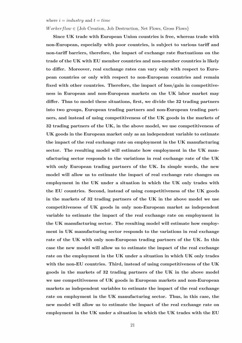
Since UK trade with European Union countries is free, whereas trade with

non-European, especially with poor countries, is subject to various tariff and

non-tariff barriers, therefore, the impact of exchange rate fluctuations on the

trade of the UK with EU member countries and non-member countries is likely

to differ. Moreover, real exchange rates can vary only with respect to Euro-

pean countries or only with respect to non-European countries and remain

fixed with other countries. Therefore, the impact of loss/gain in competitive-

ness in European and non-European markets on the UK labor market may

differ. Thus to model these situations, first, we divide the 32 trading partners

into two groups, European trading partners and non-European trading part-

ners, and instead of using competitiveness of the UK goods in the markets of

32 trading partners of the UK, in the above model, we use competitiveness of

UK goods in the European market only as an independent variable to estimate

the impact of the real exchange rate on employment in the UK manufacturing

sector. The resulting model will estimate how employment in the UK man-

ufacturing sector responds to the variations in real exchange rate of the UK

with only European trading partners of the UK. In simple words, the new

model will allow us to estimate the impact of real exchange rate changes on

employment in the UK under a situation in which the UK only trades with

the EU countries. Second, instead of using competitiveness of the UK goods

in the markets of 32 trading partners of the UK in the above model we use

competitiveness of UK goods in only non-European market as independent

variable to estimate the impact of the real exchange rate on employment in

the UK manufacturing sector. The resulting model will estimate how employ-

ment in UK manufacturing sector responds to the variations in real exchange

rate of the UK with only non-European trading partners of the UK. In this

case the new model will allow us to estimate the impact of the real exchange

rate on the employment in the UK under a situation in which UK only trades

with the non-EU countries. Third, instead of using competitiveness of the UK

goods in the markets of 32 trading partners of the UK in the above model

we use competitiveness of UK goods in European markets and non-European

markets as independent variables to estimate the impact of the real exchange

rate on employment in the UK manufacturing sector. Thus, in this case, the

new model will allow us to estimate the impact of the real exchange rate on

employment in the UK under a situation in which the UK trades with the EU

21

and non-EU countries at a time, but we assume that the fluctuations in the

exchange rates of UK with EU countries do not affect the trade with non-EU

countries or the other way round. In this case the empirical model takes the

form as written below in equation (2.3.22).

Workerflowit = β0 + β1Jobcreationit−1 + β2Jobdestructionit−1

+ β3Avgwageit + β4GDPgrowtht + β5Salesgrowthit

+ β6Competitiveness(EU)it + β7Competitiveness(non− EU)it


In fact, world trading markets are interlinked with each other and the effects of a shock

in one market may be transmitted to other markets. The linkages between the different

markets may change the pattern of job flows in trading economies in response to a shock

to the real exchange rate. In the same vein, a shock to UK trade with EU countries may

change the volume of UK trade with non-EU countries or the other way round. Thus, we

add an interaction term of EU and non-EU competitiveness in model (2.3.22) to capture

the interaction between the EU and non-EU markets and their combined effect on changes

in employment in UK manufacturing. The model (2.3.22) changes to equation (2.3.23)

given below.

Workerflowit = β0 + β1Jobcreationit−1 + β2Jobdestructionit−1

+ β3Avgwageit + β4GDPgrowtht + β5Salesgrowthit

+ β6Competitiveness(EU)it + β7Competitiveness(non− EU)it

+ β8Competitiveness(EU)it × Competitiveness(non− EU)it


2.3.3 Construction of Variables

We use a procedure similar to that of Davis et al. (1996) to calculate job flows: job

creation, job destruction, gross job flows and net job flows. Let the level of employment

in a firm in period t is eft and ∆eft is the change in employment between the period t

and t− 1. S+ and S− are the groups of firms with ∆eft > 0 and ∆eft < 0 respectively, in

industry S. To get job creation, we add up all the changes in employment in S+ group.

For job destruction, we sum all the changes in employment in S− group. The size of

the firm xft is measured as the average employment between the period t and t − 1, i.e.

xft = 0.5(eft + eft−1). Accordingly, industry size is obtained by summing up average firm

employment across the industry, i.e. Xst =∑xft

22

With regard to job flow rates, job creation, and job destruction flow rates are calculated

as the size-weighted average of the change in employment, using the formula given below.

JCst =∑fεS+

gftxftXst

(2.3.24)

JCst =∑fεS−

gftxftXst

(2.3.25)

where gft = ∆(eft)xft is the growth rate of employment in firm f at time t. The sum of

the job creation (JC) and job destruction (JD) gives total job reallocation or gross job

flows (GFR) in the industry S and the difference of JC and JD gives net changes in the

employment or net job flows (NFR) in the industry S.

Following Moser et al. (2010), we employ a real exchange rate index based on the wage

cost of the firm as the explanatory variable in the model to capture how fluctuations in real

exchange rates affect firms’ employment decisions. The real exchange rate is measured as

the UK’s average hourly wage cost in manufacturing relative to the trade-weighted average

hourly wage cost across the UK’s trading partners as below:

Real Exchange Rate = (Wage Cost)t =∑j⊂C

(Hourly Wage Cost in UK)t(Hourly Wage Cost)jt

× (Exports)jt∑iεC(Exports)it

In our analysis, a shock to the real exchange rate means a large increase/decrease

in the hourly wage average cost in the UK manufacturing sector relative to

the trade-weighted average wage cost across the UK’s trading partners. Fluc-

tuations in the real exchange rate affect employment through three channels

namely the export channel, import channel and imported inputs channel. Note

that, a rise in the real exchange rate means a rise in the cost of the produc-

tion and reduction in the profitability of a firm if the prices of the products

which it produces remain constant. The rise in real exchange rate may have

no impact on the employment if a firm is ready to reduce its profit and does

not increase the prices of its product when it faces the rise in relative wage

cost. The firm may not increase the prices of its products if it expects that

the rise in the real exchange rate is not permanent. But if a firm shifts all or

a portion of the rise in the cost of production to the prices of the product it

produces, then, the rise in the real exchange rate may lead to a reduction in

employment. This reduction in employment in response to a rise in the real

exchange rate can occur through any or all three channels given above.

In the export exposure channel, a rise in real exchange rate increases the

prices of exports and reduces the demand for goods being sold in interna-

23

tional markets. Now firms have two choices: first, they can go for piling up

their stocks and inventories and keep on producing their products at the level

at which they were producing before the rise in real exchange rate. Second,

if they do not increase their stocks and inventories and opt to reduce their

output when they face a reduction in demand for their products in interna-

tional markets. In the first case there will be no impact of a rise in the real

exchange rate on employment but in the second case a rise in the real ex-

change rate reduces the employment. So the export exposure channel have

negative impact of fluctuations in real exchange rate on employment. In the

import exposure channel, a rise in the cost of production due to a rise in real

exchange rate increases the prices of domestic products and makes imported

products relatively cheaper. This again leads to a decrease in the demand for

goods produced locally and increases the demand for imported goods. Partic-

ularly, the demand for goods whose cheaper imported substitutes are available

will decrease leading to a decrease in output and employment of the domestic

firms. So, the import exposure channel have negative impact of fluctuations

in real exchange rate on employment.

In the imported input channel, a rise in real exchange rate makes the

imported inputs cheaper. The firms can control the cost of production by

using the imported inputs. In this case impact of a rise in real exchange rate

on employment can be positive depending on the proportion of the imported

inputs being used in the production process.

So the net effect of fluctuations in the real exchange rate on employment

depends on the magnitudes of these three effects. However, in this chapter,

we focus only on the export exposure channel of the impact of the fluctuations

in the real exchange rate on employment because we do not have data on

industry level imports and the use of imported inputs.

Although the fluctuations in the real exchange rate affect employment

through three channels given above, we focus only on the export channel while

estimating the impact of real exchange rate on employment in the UK man-

ufacturing sector because we do not have the data on industry-level imports

and the data on use of industry-level imported inputs.

The wage cost(real exchange rate) and job creation move in opposite directions. How-

ever, wage cost and job destruction move in the same direction. Therefore, we expect that

an appreciation of the real exchange rate decreases the job creation rate and increases the

job destruction rate. In addition, the real exchange rate as measured in the above formula

indicates that for a given shock to the real exchange rate, employment fluctuates more in

24

the firms that have a higher export share. Thus, we expect that labor employed in the

more open firms is more exposed to external shocks, such as swings in real exchange rates.

Changes in the real exchange rates alter the relative prices and consequently, the compet-

itiveness of firms in international markets changes. So, to calculate the competitiveness

of the industry in the global market, we have interacted openness of the industry with

changes in the real exchange rate from year t to t− 1.

Competitivenessit = 4(Wage Cost)t ×Opennessit

where, openness is defined as the average share of exports in total revenues in year t

and t− 1, and it is calculated by using the formula given below

Opennessit =1

2

t−1∑τ=t−2

Exportsit(Total Revenues)it

We expect a positive coefficient of competitiveness for job creation and a negative

coefficient for job destruction. Regarding the coefficients of competitiveness for gross and

net job flows, we make no prior judgment. In the case of GDP growth rate and sales

growth rate, we expect a positive coefficient for job creation and a negative coefficients for

job destruction.

The other variables used in the analysis are defined as follows:

Hourly wage costs: Hourly compensation costs for production workers in U.S. dollars

in country j in year t.

Exports: Exports from the UK to country j in year t. We use total UK exports to

calculate real exchange rate. To calculate openness of the industry, we use firm level

exports.

Real GDP growth: Nominal GDP growth in the UK in year t, deflated by consumer

the price index.

Sales growth: Growth of total revenues from year t− 1 to t.

Avg. wage: Total wage sum in reporting year t divided by total employment in year t.

2.3.4 Data Sources

The data used in this Chapter are taken from various sources. To calculate job creation,

job destruction, gross job reallocation and net change in employment, firm-level data on

employment are obtained from the Financial Analysis Made Easy (FAME) on-line data

base. Firm level exports, sales, capital and wages and salaries are also extracted from the

same source. Researchers point out some problems with FAME data set, for

example Harris and Li (2007) compared the Annual Respondents Database

25

(ARD) and FAME data sets and report, the FAME database is unrepresenta-

tive of small- to medium-sized enterprises and therefore cannot produce results

that can be generalized to the UK level. In pointing out that FAME is biased

towards large enterprises Harris and Li (2007) define a firm as a small firm

if it employs less than 13 employees, a firm as a medium firm if it employs

between 13 and 66 employees and a firm as a large firm if it employs more than

66 employees. However, if we use the European Union definition of firms clas-

sification then FAME data gives a good representation of the small, medium

and large firms. According to the European Classification of firms, a firm is

termed as a small firm if it employs less than 50 people, a firm is termed as

a medium firm if it employs 50 to 249 people and a firm is termed as a large

firm if it employs 250 or more people. Moreover, many researchers like Faggio

et al. (2010), Greenhalgh and Rogers (2006), Bridges and Guariglia (2008),

Liu et al. (2000), Girma et al. (2008), Draca et al. (2008) and Greenaway et al.

(2007) have used the data extracted from FAME database for their firm-level

studies for the UK. Our sample size consists of firms of twenty two industries

of the UK manufacturing sector. These 22 industries give a good representa-

tion of small, medium and large firms. Table 1 and Figure 1 show distribution

of the firms into small, medium and large in each industry. Table 1 shows that

the share of small and large firms are almost similar in most of the industries.

Only in the cases of industries 16, 34 and 35 are the shares of large firms much

higher than the share of small firms. However, the total number of firms in

these industries is low, particularly in industry 16 the total number of firms

is just 161. The share of medium sized firms in each industry is higher than

the share of small and large firms in all the industries except in industry 16

in which the share of large firms is the higher than the share of medium and

small firms.

The firm-specific information available at FAME gives us an opportunity to extend

our analysis for exporting and non-exporting industries. To accomplish this purpose, we

define an exporting industry as a group of firms in an industry who sell their product

in international markets. In contrast, we define non-exporting industry as a group of

firms in an industry who sell their products only in domestic markets. More precisely, the

FAME data set allows us to capture the behavioral response of firms who are involved in

international trade, and the firms who sell only in the domestic markets, to an exogenous

shock.

Another important variable which affects the decisions of firms regarding employment

is the hourly wage cost. This is taken from the United States Bureau of Labor Statis-

26

Table 1: Distribution of Firms in 22 Industries of the UK ManufacturingSector

No. of Firms Shares

Industry Total Small Medium Large Small Medium Large

15 12553 2682 5686 4185 21.37 45.30 33.3416 161 37 37 87 22.98 22.98 54.0417 3774 740 2099 935 19.61 55.62 24.7718 2157 694 922 541 32.17 42.74 25.0819 728 108 426 194 14.84 58.52 26.6520 2986 676 1722 588 22.64 57.67 19.6921 3727 692 2137 898 18.57 57.34 24.0922 13454 3983 6534 2937 29.60 48.57 21.8323 661 203 287 171 30.71 43.42 25.8724 11296 3194 5115 2987 28.28 45.28 26.4425 7630 1457 4309 1864 19.10 56.47 24.4326 4298 978 2057 1263 22.75 47.86 29.3927 4087 1128 1993 966 27.60 48.76 23.6428 18416 4187 10743 3486 22.74 58.34 18.9329 11525 3364 5334 2827 29.19 46.28 24.5330 2264 680 1017 567 30.04 44.92 25.0431 7739 1942 3879 1918 25.09 50.12 24.7832 4217 954 2217 1046 22.62 52.57 24.8033 5898 1775 2820 1303 30.09 47.81 22.0934 3385 371 1626 1388 10.96 48.04 41.0035 3059 633 1331 1095 20.69 43.51 35.8036 14403 3509 8044 2850 24.36 55.85 19.79

According to European Classification of firms, a firm is termed as a small firm if it employs less than 50people. a firm is termed as a medium firm if it employs 50 to 249 people and a firm is termed as a largefirm if it employs 250 or more people.UK SIC 2003 classification is used for industry classification coding. See Table A.7 in the Appendix A forindustry code explanation.

Figure 1: Share of Firms in 22 industries of UK Manufacturing Sector

0.00

10.00

20.00

30.00

40.00

50.00

60.00

70.00

15 16 17 18 19 20 21 22 23 24 25 26 27 28 29 30 31 32 33 34 35 36

Shares

Industry

Small

Medium

Large

Small=Firm employing less than 50 people.

Medium= Firm employing 50 to 249 people.

Large= Firm employing 250 or more people.

tics (BLS). BLS provides hourly wage costs for 32 countries from four different regions:

Americas, Europe, Asia and Oceania. We have divided these 32 countries into two major

27

groups: European and non-European to measure how changes in wage costs in the UK

relative to other countries affect employment in the UK manufacturing (see Table 2 for

UK trading partners).

Table 2: The UK Major Trading Partners

No European Trading partners No non-European Trading Partners

1 Austria 1 United States2 Belgium 2 Brazil3 Czech Republic 3 Mexico4 Denmark 4 Australia5 Finland 5 China, P.R: Hong Kong6 France 6 Israel7 Germany 7 Japan8 Hungary 8 Korea Republic of9 Ireland 9 New Zealand10 Italy 10 Philippine11 Luxembourg 11 Singapore12 Netherlands 12 Sri Lanka13 Norway 13 Canada14 Poland16 Portugal17 Spain18 Sweden19 Switzerland

Also note that the data on hourly wage costs are available only for these 32 countries.

Further note that more than 80 percent of UK exports flow to these countries (see Table

3). More than 96 percent of UK total exports to European markets goes to the countries

we have included in our sample. Similarly, more than 59 percent of total UK exports to

non-European countries goes to the countries we have selected as non-European trading

partners of the UK.

We have exploited hourly wage costs to calculate real exchange rates for the UK with

other European and non-European countries and the competitiveness of the exports of

the UK in European and non-European countries’ markets. Details of the construction of

the real exchange rate and competitiveness are given in the variable construction section.

Other macroeconomic variables used in this study are the GDP growth rate and CPI.

The data on GDP growth rate and CPI are extracted from World Development Indicator

(WDI) 2009. Similarly, data on UK exports to her various trading partners are taken from

the United Nations on-line data base; UN COMTRADE. This analysis covers the time

period from 1999 to 2010.

28

Table 3: UK Export Share to EU and non-EU Countries

Year EU non-EU Selected 32 Selected EU Selected non-EUCountries Countries Countries Countries Countries

1999 63.66 36.34 86.72 97.65 67.592000 62.06 37.94 86.61 97.49 68.802001 59.91 40.09 84.30 97.52 64.552002 61.36 38.64 85.13 97.33 65.772003 59.28 40.72 83.17 96.97 63.082004 57.93 42.07 81.54 96.82 60.522005 57.63 42.37 80.85 97.02 58.852006 60.81 39.19 81.83 96.83 58.562007 60.58 39.42 81.90 96.71 59.142008 59.78 40.22 80.84 96.54 57.512009 58.23 41.77 80.89 96.50 59.14

Note: See Table 2 for EU and non-EU trading partners of the UK.All figures are in percentage.

2.3.5 At First Glance

Although our data cover only 12 years from 1999 to 2010, a relatively short time period,

our variables of interest including the real exchange rate, GDP growth rate, employment,

exports and sales exhibit considerable variations. Below we explain how the real exchange

rate of the UK have behaved throughout the sample period and then we present the

summary statistics of the other variables included in the model.

According to Cobham (2002) in the presence of separate currencies with

variable exchange rates for different countries, the exchange rate is seen as

an important adjustment mechanism and an important policy tool in trans-

mitting/absorbing the effects of an external shock under the flexible exchange

rate regimes. However, other researchers like Buiter (2000) point out that

the exchange rate itself is a source of external asymmetric shocks therefore

he prefers fixed exchange rate regimes and favors the fixed exchange rate and

giving up the adjustment mechanism that works through flexible exchange

rates.

The UK is a good example of the flexible and fixed exchange rate regimes

because to be the part of European Monetary System (EMS) the UK entered

into the European Exchange Rate Mechanism (ERM) program in October

1990 and adopted the fixed exchange rate system. However, the UK left the

ERM program within two years in September 1992 and came back to flexible

exchange rate regime because the pound sterling came under the pressure of

speculators.

As the exchange rate of a country appreciates or depreciate and adjusts

29

in short-run under the flexible exchange rate mechanism in response to the

nature of an external shocks such as portfolio shock therefore it automatically

move towards some long-run equilibrium. The overvalued valued currencies

depreciate and undervalued currencies appreciate and move along their long-

run equilibrium values. The large fluctuations in the values of a currency in

terms of other currencies in which substantial deviations from the average

value occurs are termed as the shock to the exchange rate.

Fluctuations in nominal exchange rates: value of currency of the country

in terms of currency of another country, brings about changes in the real

exchange rate: cost of foreign goods in terms of domestic goods. According to

Cobham (2002) for UK, in short-run the causality runs from nominal exchange

rate to real exchange rate and has marked the period of 1975 to 2000 as

a period of strong depreciations in the nominal exchange rate of the UK.

Moreover, he marked the trends of appreciations in the real exchange rate

of the UK over the period from 1979 to 1981 and over the period from 1996

to 1998. During this period the fluctuations in the real exchange rate were

similar to the changes in the nominal exchange rate, however, the changes in

real exchange rates were preceded by the fluctuations in nominal exchange

rates.

Since our objective is to measure the impact of the fluctuations in the real

exchange rates on the employment in the UK manufacturing sector, therefore,

we use the real exchange rate based on trade-weighted labor cost in UK man-

ufacturing sector relative to labor costs in the manufacturing sectors of the

trading partners of the UK. Figure 2 shows the wage costs in manufacturing

sector based real exchange rate of the UK over the period of the 1999 to 2010.

The trends in real exchange rate suggests the large overvaluation during the

period from 1999 to 2001 and the large undervaluation during the period from

2008 to 2010. Wren-Lewis and Britain (2003) and Cobham (2006) reported

that pound sterling was 16 percent overvalued against euro and 10 percent

overvalued against the dollar in 2002. Furthermore, Cobham (2006) points

out that these overvaluations of the sterling had an adverse impact on the

tradable sector. Overall, Figure 2 and Figure 4 suggest that overvaluations of

the sterling from 2006 to 2007 had adversely affected the UK exports. Simi-

larly, the trends in real exchange rate also suggests the small undervaluation

during the period from 2002 to 2003 and the small overvaluation during the

period from 2006 to 2007. Overall, Figure 2 suggest that real exchange rate

of the UK had been oscillating around its average value of the whole sample

30

period. The movements in the real exchange rate of the UK during 1999 to

2010 can be divided into three segments: first, the period of depreciation from

1999 to 2003, second, the period of appreciation from 2003 to 2007 and third,

again the period of depreciation from 2007 to 2010.

Figure 2: Real Exchange Rate based on the Wage Costs in ManufacturingSector of the UK from 1999 to 2010

0.60

0.70

0.80

0.90

1.00

1.10

1.20

1999 2000 2001 2002 2003 2004 2005 2006 2007 2008 2009 2010

RER RER average 1999-‐2010 = 0.98 RER average 1999-‐2010 + 5% = 1.03 RER average 1999-‐2010 -‐ 5% = 0.93

However, Figure 3 shows that trade-weighted real exchange rate of the UK

was relatively less volatile and had oscillated within the band of five percent

around the mean value of the real exchange rates for the period starting from

1999 to 2008. The trend in trade weighted real exchange rate indicates the

large undervaluation from 2008 and onward. According to Cobham (2002) the

real exchange rate based on wage costs in manufacturing sector reflects the

variations in the mark ups that affect the competitiveness of the UK goods

traded in the global markets, therefore, the trends in real exchange rates shown

in Figures 2 and 3 may indicate that the fluctuations in the competitiveness

of the UK goods in international markets, which in turn affects the exports,

output and employment.

Figures 4, 5, 6 and 7 show variations in real exports, real exchange rate

with 32 trading partners, real exchange rate with non-EU trading partners

and real exchange rate with EU trading partners.

Figures 4, 5, 7 and 18 in Appendix A show real exchange rate of the UK

with 32 trading partners, with non-EU trading partners, with EU trading

partners and with top 5 UK trading partners. Figures 4, 5 and 7 suggest

that total exports and real exchange rate with 32 trading partners and real

exchange rate with EU trading partners move in opposite directions. However,

Figure 6 seems to suggest that total exports and the real exchange rate with

non-EU trading partners move in same direction. This may be driven by the

31

Figure 3: Trade-weighted Real Exchange Rate of the UK from 1999 to 2010

1.100

1.150

1.200

1.250

1.300

1.350

1.400

1999 2000 2001 2002 2003 2004 2005 2006 2007 2008 2009

RER 32

RER 32 average 1999-‐2010 + 5% = 1.346

RER 32 average 1999-‐2010 -‐ 5% = 1.217

RER 32 average 1999-‐2010=1.282

Figure 4: Total Exports of the UK from 1999 to 2010

0

5

10

15

20

25

30

35

40

45

50

1999 2000 2001 2002 2003 2004 2005 2006 2007 2008 2009 2010

Exports are in $10M and at 2005 prices

fact that labor compensation cost in UK manufacturing sector is relatively low

as compared to the EU and non-EU trading partners. Our measure of real

exchange rate is based on compensation cost which in fact has risen over the

time but remained less as compared to EU and non-EU trading partners of

the UK. Figures 8,9 and 10 shows that compensation costs of the UK and its

5 major trading partners. The trend in these Figures shows that the UK is

relatively a low cost country. Figure 10 shows that before 2003, hourly labor

compensation cost in the UK was low as compared to compensation costs in

non-EU trading partners but higher as compared with the compensation costs

in EU trading partners. From 2003 to 2007 labor compensation cost in UK

was similar to its trading partners but after 2007 it has become higher in both

EU and non-EU trading partners of the UK. Comparing Figures 5, 6, 7 in the

main text and Figure 16 in Appendix A suggests that the real exchange rate and average

32

Figure 5: UK’s Real Exchange Rate with selected 32 Trading Partners from1999 to 2010

0

0.2

0.4

0.6

0.8

1

1.2

1999 2000 2001 2002 2003 2004 2005 2006 2007 2008 2009 2010

RER 32

Figures are in US Dollars at 2005 prices

Figure 6: UK’s Real Exchange Rate with selected non-EU Trading Partnersfrom 1999 to 2010

0

0.2

0.4

0.6

0.8

1

1.2

1999 2000 2001 2002 2003 2004 2005 2006 2007 2008 2009 2010

RER Non EU


export shares in total sales move in opposite directions, and that the real exchange rate

appears a prominent variable in explaining current export shares in total sales. The trend

in the real exchange rate and export shares in total sales suggests that real exchange rate

fluctuations precede changes in export shares in total sale. So, in the light of these figures

we can say that UK manufacturing industries may sign future export contracts on the

basis of the current real exchange rate.

Figure 17 in Appendix A displays average employment in the UK manufacturing sector.

In the light of Figure 17 in the Appendix A, we can see that average employment in

this sector steadily decreased over time. Specifically, the continuous downward trend

in average employment in the last decade seems to suggest that average employment is

uncorrelated with the real exchange rate. However, when we split the manufacturing sector

33

Figure 7: UK’s Real Exchange Rate with selected EU Trading Partners from1999 to 2010

0

0.2

0.4

0.6

0.8

1

1.2

1999 2000 2001 2002 2003 2004 2005 2006 2007 2008 2009 2010

RER EU


into exporting and non-exporting industries, the trends in average employment shows its

linkages with the real exchange rate more clearly. For instance, the appreciation in the

real exchange rate in the late nineties is escorting the decline in employment in exporting

industries and the rise in employment in non-exporting industries in 2000.

Table 4: Summary Statistics (All Industries)

Year Total GDP Sales Export Job Job Net Gross

Employment Growth Growth Share Creation Destruction Flows Flows

1999 375320 3.47 27.542000 388528 3.92 17.84 27.66 6.37 15.61 -9.24 21.992001 403820 2.46 18.46 19.67 5.03 9.41 -4.39 14.442002 390478 2.10 0.37 20.50 4.59 9.37 -4.78 13.952003 370680 2.82 12.19 19.67 3.20 8.62 -5.43 11.822004 352289 2.76 1.29 22.26 4.09 6.42 -2.33 10.522005 339726 2.17 6.85 17.58 4.75 6.97 -2.22 11.722006 333018 2.85 0.62 19.77 4.96 6.09 -1.13 11.052007 326934 2.56 4.42 18.24 4.91 5.66 -0.74 10.572008 325298 0.55 13.42 17.74 5.82 5.00 0.82 10.812009 270298 -4.92 -141.54 31.30 2.34 7.19 -4.85 9.53

Note: See Table 2 for EU and non-EU trading partners of the UK.All figures except total employment are in percentage.

34

Figure 8: Average Hourly Compensation Cost in Manufacturing Sectors ofthe UK and UK’s top 5 Trading Partners from 1999 to 2010

88

89

90

91

92

93

94

95

96

97

98

99

United States

Germany

Ireland

Italy

Netherlands

United Kingdom

Compensaion Cost is in US Dollars at 2005 prices and includes Pay for time worked

, Social Insurance and Directly paid benefits.

Figure 9: Hourly Compensation Cost in Manufacturing Sectors of the UK andUK’s Trading Partners from 1999 to 2010

0

20

40

60

80

100

120

140

160

1999 2000 2001 2002 2003 2004 2005 2006 2007 2008 2009 2010

UK

32 Partners

EU Partners

Non-EU Partners

Figures are in US Dollars at 2005 prices. Per Hour Compensation Cost is includes Pay

for time worked, Social Insurance and Directly paid benefits

35

Figure 10: Hourly Compensation Cost in Manufacturing Sectors of the UKand UK’s top 5 Trading Partners from 1999 to 2010

0

20

40

60

80

100

120

140

160

1999 2000 2001 2002 2003 2004 2005 2006 2007 2008 2009 2010

United States

Germany

Italy

Ireland

Netherlands

UK

Figures are in US Dollars at 2005 prices. Per Hour Compensation Cost is includes Pay

for time worked, Social Insurance and Directly paid benefits.

Table 5: Summary Statistics (Exporting Industries)

Year Total GDP Sales Export Job Job Net Gross

Employment Growth Growth Share Creation Destruction Flows Flows

1999 190213 3.47 48.212000 217847 3.92 14.32 49.34 7.30 7.47 -0.16 14.772001 199208 2.46 -15.68 45.95 4.54 8.57 -4.02 13.112002 206181 2.10 8.87 47.01 7.48 11.08 -3.59 18.562003 196554 2.82 -133.17 48.48 3.63 6.66 -3.03 10.292004 188833 2.76 7.74 49.40 3.36 6.91 -3.55 10.272005 184639 2.17 -54.86 48.25 5.05 5.12 -0.07 10.172006 174848 2.85 1.57 50.94 5.18 5.33 -0.15 10.512007 171241 2.56 0.16 50.77 5.60 3.78 1.82 9.382008 165619 0.55 4.88 52.55 5.68 4.26 1.42 9.952009 161019 -4.92 -6.65 56.78 2.97 7.41 -4.44 10.39

Note: See Table 2 for EU and non-EU trading partners of the UK.All figures except total employment are in percentage.Note that we define an exporting industry as the group of firms in an industry that sell all or a portionof their output in foreign markets. Moreover, if a firm exports in some years and does not export in otheryears, in this case we include this particular firm in exporting firms’ group in the years in which it has soldall or a portion of its output in foreign markets, and in all other years we include this particular firm innon-exporting firms’ group because this firm’s exports are zero in these years.

36

Table 6: Summary Statistics (Non-Exporting Industries)

Year Total GDP Sales Job Job Net Gross

Employment Growth Growth Creation Destruction Flows Flows

1999 185107 3.472000 170681 3.92 13.66 4.80 26.39 -21.59 31.192001 204611 2.46 33.56 6.49 10.04 -3.55 16.522002 184298 2.10 -1.14 3.31 7.53 -4.22 10.852003 174126 2.82 11.92 3.19 11.12 -7.93 14.312004 163456 2.76 -10.09 5.29 6.88 -1.58 12.172005 155087 2.17 13.88 4.46 9.27 -4.81 13.722006 158170 2.85 -23.85 4.86 7.45 -2.58 12.312007 155693 2.56 8.85 4.50 9.10 -4.61 13.602008 159679 0.55 14.44 8.69 6.44 2.25 15.132009 109278 -4.92 -305.86 1.92 7.77 -5.85 9.69

Note: See Table 2 for EU and non-EU trading partners of the UK.All the figures except total employment are in percentage.Note that we define non-exporting industry as the group of a firms in an industry that do not sell theirout put in the foreign markets.

Table 7: Average Job Creation, Job Destruction , Net Flows, Gross Flows,Sales, Exports and Wages in UK Manufacturing Industries from 1999-2010

IndustryCode JC JD NF GF Sale Export Wages

15 50983.08 95592.34 -44609.25 146575.4 3697189 171874.6 122165.116 5597.333 3591.583 2005.75 9188.917 291182.3 60399.43 14601.9717 5803.333 11071.58 -5268.25 16874.92 96932.39 20055.54 12565.9718 4503.417 8552 -4048.583 13055.42 70634.84 7543.109 7467.33719 892.1667 2388.5 -1496.333 3280.667 40240.04 7230.404 3196.64620 2846.833 8060.167 -5213.333 10907 85744.76 4543.737 8847.78821 3799.417 9297.667 -5498.25 13097.08 506284.3 36815.36 22395.5622 22281.5 34270 -11988.5 56551.5 1260667 178784.6 100786.723 3445.333 7741.083 -4295.75 11186.42 2321497 504470.7 58681.8124 18202.83 50266.42 -32063.58 68469.25 3272974 411923.3 119461.825 8148.583 20784.83 -12636.25 28933.42 480903.2 74528.7 36091.4726 8039.583 26072.25 -18032.67 34111.83 1543351 62480.46 34576.4427 6096.75 11961.67 -5864.917 18058.42 390737.8 142946.2 30326.7428 36356.33 54847.42 -18491.08 91203.75 995959.7 297853.5 126096.829 26240.75 58231.42 -31990.67 84472.16 1107337 426489.7 127410.930 7200.083 6551.25 648.8333 13751.33 783334.3 62050.59 26499.7831 15751.67 35525.25 -19773.58 51276.92 605052.3 144426.8 54367.8732 14031.17 13341.83 689.3333 27373 711675.7 238626.1 46822.8933 16995.83 21788.42 -4792.583 38784.25 566316.6 201236.1 61050.1634 7424.75 22025 -14600.25 29449.75 492274.6 92554.8 42116.7435 14638.58 11589.75 3048.833 26228.33 406481.1 205955.2 68437.1836 17701.67 28204.67 -10503 45906.33 685707.6 106033.4 68424.65

UK SIC 2003 classification is used for industry classification coding.Wages, Sales and Exports are at 2005 prices.see Table A.7 in the appendix for industry code explanation

37

Table 8: UK Real Exchange Rate with Selected Countries

Year Selected 32 Selected EU Selected non-EUCountries Countries Countries

1999 0.996 1.036 0.8942000 1.040 1.120 0.8552001 1.027 1.103 0.8422002 1.014 1.070 0.8742003 0.960 0.976 0.9242004 0.989 0.984 1.0002005 1.000 1.000 1.0002006 1.015 1.011 1.0282007 1.035 1.013 1.0912008 0.921 0.884 1.0132009 0.808 0.784 0.8642010 0.809 0.805 0.819

Note: See Table 2 for selected EU and non-EU trading partners of the UK.Real exchange rate figures are calculated using 2005 as base year.

38

It seems that in the early 2000s, fluctuations in the real exchange rate are followed by

the shifting of resources from exporting industries to non-exporting industries. Thus, the

fall of employment in trading industries appears to be absorbed by non-trading industries.

However, after 2002 employment in both the exporting and non-exporting industries falls

which gives the impression that the UK manufacturing sector is contracting. Moreover,

summary statistics given in Tables 4, 5, 6 and 7 also show that UK manufacturing sector

is contracting. Employment growth in all the industries except industries 16, 30, 32, and

35 net employment is negative. Table 7 indicates that 18 out of 22 industries of the UK

manufacturing sectors show a decline in average employment. Tables 4, 5, 6, 7 and 8

indicate that the impact of the real exchange rate on aggregate employment is small. So,

the summary statistics given in Tables 4, 5, 6, 7 and 8, and the trends in Figures 4, 5, 6 and

7 given above and Figures 16 and 17 in Appendix A reveal that the employment and real

exchange rate are interconnected and labor adjustment cost driven by the exchange rate is

worthy of analysis. Industry-wise exports are shown in Figure 19 in Appendix A. Figure

19 in Appendix A indicates that the industrial exports of the UK manufacturing sector

vary across the industries and over the time. Particularly the exports of the industries 15,

16, 17, 20, 21, 22, 23, 26, 30 and 32 show a considerable variations in their sales in the

foreign markets.

2.3.6 Estimation of the Model

The models proposed in equations (2.3.21), (2.3.22) and (2.3.23) are the dynamic panel

models in which the current realization of the job flows are influenced by the previous

period job flows. These models are first order autoregressive (AR1) panel data models

because only the first lag of the dependent variable appears as an explanatory variable in

the models. The general form of first order autoregressive (AR1) panel data models can

be written as follows:

yit =

ρ∑i=1

αiyi,t−1 + β0 + β1xit + β2zit + µi + τt + εit (2.3.26)

where t = 1 + ρ, ....., T years, i = 1, ...., N industries, yit is the job flow rate in industry

i at time t, xit is a vector of pre-determined control variables, zit is a vector of other

exogenous variables, µi is an unobserved time-invariant industry-specific fixed effects, τt

is time specific fixed effects and εit is an error term. αi, ı=1,.......,ρ and βj , j=0,1,2 are

the regression coefficients with |∑αi| ≤ 1. Blundell and Bond (1998) focused on initial

conditions to estimate the parameters of dynamic models such as this. In these initial

conditions which implies that moment restrictions are sufficient to estimate αi for T ≥ 3

Blundell and Bond (1998) assume that µi and εit are independently distributed across

the i and have the familiar error components structure in which E[µi] = 0, E[εit] = 0,

39

E[µiεit] = 0, for t = 1 + ρ, ......, T years, i = 1, ......, N industries. They also assumed that

error εit are serially uncorrelated and that the initial conditions yit are predetermined.

That is E[εitεis] = 0 for i = 1, ......, N and s 6= t and E[yi1εit] = 0 for t = 2, ......, T years,

i = 1, ......, N industries.

Estimating such a dynamic regression model of industrial job flow rates controlling for

different possible determinants on a panel of heterogeneous industries may raise econo-

metric problems which need to be care of while estimating these models. These problems

include:

• Omitted variable or time invariant industry specific characteristics (fixed effects) µi

may be correlated with the explanatory variables and cause biased estimation.

• The idiosyncratic disturbance term εit may have individual specific pattern of het-

eroscedasticity.

• Due to shorter time and larger industry dimension of the panel data, a shock to

industry specific effects may not dissipate with time and hence cause significant

correlation of yit−1 with the error term.

• Besides yit−1, some other regressors may be endogenous and thus may be correlated

with the error term in the regression.

All these problems make OLS estimates biased and inconsistent. Particularly the en-

dogeneity of yi,t−1 to the industry specific fixed effect µi makes yi,t−1 correlated with error

term and ultimately makes OLS estimates upward biased and inconsistent (Presbitero,

2008). Therefore, a possible solution to get consistent estimates is Generalized Method

of Moments (GMM) which takes care of these issues when estimating the dynamic panel

model. Specifically, Arellano and Bover (1995) / Blundell and Bond (1998) propose Sys-

tem GMM to estimate the dynamic panel model such as given in equation in 2.3.26.

Basically, System GMM estimate the dynamic panel model using a system of two simul-

taneous equations, one in levels and other in first differences. Moreover, System GMM

uses instruments while estimating the regression model, where the instrument used in level

equations are lagged first differences and instruments used in first difference equation are

lagged levels of the series. Through this System GMM controls for potential endogene-

ity problem and controls for possible correlation between the unobserved, time invariant

cross-section specific effects and any of the explanatory variable and gives consistent es-

timates. Solomon (2010) describes three advantages of using System GMM estimator to

estimate the dynamic panel model.

• First, System GMM controls for the potential endogeneity arising from the explana-

tory variables in the model.

40

• Second, System GMM control for the possible correlation between the unobserved,

time invariant cross-section specific effects and any of the explanatory variable.

• Finally, System GMM is good in dealing with short and persistent data sets and

it does not suffer from the weak instrument problem which could arise from such a

data set.

2.4 Empirical Results

2.4.1 All Industries

This section discusses the results for all industries of the UK manufacturing sector. From

all industries of the UK manufacturing sector we mean that when we estimate the empirical

model using the data of 22 industries of the UK manufacturing sectors included in our

sample. Table 9 reports the estimation results when the dependent variable is net job

flows. Column 1 contains the results when we consider 32 trading partners of the UK as

one group while calculating the real exchange rate. This column shows how employment

responds to variations in the real exchange rate of the UK with major trading partners

of the UK. Column 2 shows the results when we consider only selected European trading

of the UK as one group while calculating the real exchange rate. Column 3 shows the

results when we consider only selected non-European trading of the UK as a one group

while calculating the real exchange rate. Column 4 shows the results when we consider

real exchange rate of the UK with both European and non-European trading partners of

the UK simultaneously. Column 5 displays the results when we consider real exchange

rate of the UK with both European and non-European trading partners along with their

interaction. All the remaining tables presented in this section are structured similarly

except that they contain as the dependent variables job creation, job destruction and

gross job flows, respectively. We have estimated these models using the Blundell and

Bond (1998) dynamic panel estimation technique, generally known as System GMM and

our main variable of interest, competitiveness, is assumed to be predetermined.

Now we discuss our findings one by one in the light of the results presented in Tables

9, 10, 11 and 12. Our first result highlights the response of net job flows to the variations

in competitiveness. Columns 1, 2 and 3 of Table 9 shows that the coefficient of compet-

itiveness is negative and statistically significant. Thus, columns 1, 2 and 3 of Table 9

indicate that a rise in competitiveness1 significantly reduces the net job flows in the UK

manufacturing sector.

1Our variable competitiveness is combination of the real exchange rate based on trade weighted relativewages and openness of the industry, therefore, when we say rise in competitiveness variable it means UKproducts are becoming less competitive in international markets due to the rise in relative wage cost ofthe UK products.

41

Table 9: Net Job Flows in Manufacturing Sector of the UK (All Industries)

Dependent Variable: Net Job Flow Rate1 2 3 4 5

L.Job Creation (-0.363)** (-0.403)*** (-0.512)*** (-0.372)** (-0.413)**(0.172) (0.151) (0.165) (0.147) (0.174)

L. Job Destruction (-0.558)*** (-0.424)** (-0.337)* (-0.351)** -0.244(-0.165) (0.171) (0.184) (0.14) (0.168)

Average Wage (-0.833) -0.516 -0.260 -0.183 -0.055(0.601) (0.548) (0.596) (0.619) (0.702)

GDP Growth 0.004** 0.003* 0.003* 0.004** 0.004**(0.002) (0.002) (0.002) (0.002) (0.002)

Size (-0.027)* (-0.029)*** (-0.035)** (-0.030)** (-0.036)**(0.014) (0.013) (0.016) (0.0146) (0.019)

Competitiveness (-0.520)**(32 Partners) (0.249)Competitiveness (-0.539)** -0.107 0.530(EU Partners) (0.252) (0.333) (0.48)Competitiveness (-0.352)*** (-0.282)* (-0.391)**(non-EU Partners) (0.118) (0.168) (0.171)Competitiveness 0.001*(Interaction) (0.001)Constant 0.056* 0.040* 0.038* 0.028 0.022

(0.024) (0.022) (0.021) (0.028) (0.021)

Arellano AR(2) Probability 0.120 0.172 0.500 0.265 0.640Hansen Test Probability 0.720 0.963 0.931 0.535 0.998Total Observation 198 198 198 198 198No. Of Groups 22 22 22 22 22Observation per group 9 9 9 9 9

Robust Standard Errors are given in parentheses.Standard Errors are clustered by industry.∗ ∗ ∗ = Significant at 1 percent. ∗∗ = Significant at 5 percent. ∗= Significance at 10 percent.

Specifically, net job flow rates are reduced by 0.520, 0.539 and 0.352 units, with a one

unit rise in the competitiveness of the UK with respect to 32 trading partners, with respect

to EU trading partners and with respect to non-EU trading partners respectively. Since

the competitiveness variable is a combination of the real exchange rate and openness,

therefore, these results imply that a rise in the real exchange rate significantly reduces

net employment in the UK manufacturing sector and this effect is more intensive in the

industries that export more. Moreover, an increase in the real exchange rate significantly

decreases net employment in UK manufacturing sector whether we consider the real ex-

change rate of the UK with respect to selected 32 trading partners, the real exchange rate

of the UK with respect to selected EU trading partners or the real exchange rate with

respect to selected non-EU trading partners. So, the real exchange rate affects net job

flows in the UK manufacturing sector negatively and significantly whether we consider 32

trading partners as a group to calculate the real exchange rate, or we split these 32 trading

partners into EU and non-EU trading partners and consider them as an individual group

42

to calculate the real exchange rate, and consider UK trade with only one group at a time.

The UK has trade ties with the EU and non-EU countries and UK exports are going

to EU and non-EU countries at the same time though the volume of exports going to

EU trading partners is considerably higher than the volume of exports going to non-EU

trading partners. Moreover, the wage cost of the UK relative to EU countries and relative

to non-EU countries also varies. Therefore, the impact of a change in the real exchange

rate of the UK with respect to EU countries may differ from the impact of a change in the

real exchange of the UK with respect to non-EU countries. To test this we have divided the

32 trading partners into EU and non-EU trading partners and calculated the real exchange

rates and competitiveness for each group and have included the competitiveness of the UK

in EU markets and the competitiveness of the UK in non-EU markets simultaneously in

the model. The results of this model are reported in column 4 of Table 9. The coefficients

of Competitiveness (EU Partners) and Competitiveness (non-EU Partners) indicate that

Competitiveness (EU Partners) and Competitiveness (non-EU Partners) both affect the

net job flows in the UK manufacturing sector negatively. However, Competitiveness (non-

EU Partners) significantly reduces net job flows in the UK and Competitiveness (EU

Partners) plays an insignificant role in determining the net employment in the UK. This

implies that when we consider the real exchange rate of the UK with EU countries and the

real exchange rate of the UK with non-EU countries then a rise in the real exchange rate

of the UK with non-EU countries significantly reduces the employment in the UK. This

also implies that a rise in wage costs of the UK relative to non-EU countries is detrimental

to employment in the UK. However, a rise in wage costs of the UK relative to the EU

countries is insignificant in explaining employment in the UK. This may due to the fact

that UK is relatively more low cost than non-European trading partners and relatively

less low cost as compared with European trading partners (see Figures 8 and 9 for the

cost comparison).

Similarly, column 5 of the Table 9 shows the results when we add the interaction of

the Competitiveness (EU Partners) and Competitiveness (non-EU Partners) in the model.

The idea behind including this interaction terms was to test whether the fluctuations in

competitiveness of UK goods in EU markets affects the competitiveness of UK goods in

the non-EU markets or the other way round and ultimately affect the job flows in the UK

or not. Results reported in column 5 of the Table 9 once again indicate that a rise in

competitiveness of the UK in non-EU markets significantly determines net employment in

the UK whereas a rise in competitiveness of the UK in EU markets does not affect net

employment in the UK. However, the positive and significant coefficient of the interaction

terms indicates that the fluctuations in competitiveness of the UK goods in EU markets

affects the competitiveness of UK goods in the non-EU markets or the other way round

43

and significantly increases job flows in the UK. This also indicates that the rise in the

competitiveness in the non-EU markets leads to increase in the jobs that firms that export

their products to the EU countries, and vice versa.

The elasticity of net employment in UK manufacturing sector to competitiveness with

respect to 32 trading partners is about seven percent(0.06). Similarly, the elasticity of

net employment in UK manufacturing sector to competitiveness with respect to European

trading partners is seven percent(0.09). However, the elasticity of net employment in UK

manufacturing sector to competitiveness with respect to non-European trading partners

is relatively less and it is four percent(0.02). These elasticities shows that other things

remaining the same, one percent change in the competitiveness leads to less than one

percent changes in the net employment in the UK manufacturing sector.

Since we define competitiveness as a product of the real exchange rate (trade weighted

wage cost of the UK relative to its trading partner) and openness (average share of exports

in total sales in last two years), therefore, our negative coefficients of the competitiveness

imply that a rise in the wage cost of the UK relative to its trading partners reduces

employment in the UK manufacturing sector. This effect becomes intensive for firms

with larger export shares. Note that this finding does not change whether we consider

all 32 sample trading partners of the UK or when we divide these 32 trading partners

into European and non-European trading partners of the UK and use European or non-

European only or both at a time as a separate group (see Columns 1, 2, 3 and 4 in Table 9)

or when we consider or European and non-European trading partners both simultaneously

and along with their interaction (see Columns 4 and 5 in Table 9).

However, the coefficient of competitiveness (EU trading partners) in Column 2 of the

Table 9 is bigger than the coefficient of competitiveness (non-EU trading partners) in

Column 3 of the Table 9. This finding suggests that as compared to a shock to UK

competitiveness in non-EU markets, a shock to UK competitiveness in EU markets affects

employment in the manufacturing sector of the UK more significantly. The difference in

the effect of a change in competitiveness of the UK with regard to European and non-

European countries on net employment exists because the UK exports more relatively to

European countries (see, Table 3). Moreover, as displayed in Column 4, when we take

into account European and non-European trading partners of the UK simultaneously,

then, a rise in UK competitiveness relative to non-European countries significantly reduces

net employment. This result suggests that employment in the UK is more sensitive to

fluctuations in exchange rates of the UK with non-European countries despite the fact

that the share of UK exports going to non-European countries is lower than the share of

UK exports going to the European countries.

Furthermore, Table 9 shows that firm-specific variables like average wages and the firm

44

size reduces the net jobs flows. However, a rise in average wages significantly decreases the

net job flows in the UK manufacturing sector. The coefficient of the average wage ranges

from -1.009 to -0.562 depending on the model specification. This implies that firms cut

down their staff when they face a higher wage cost. Moreover, the negative coefficients

of size in all the models we have estimated show that net job flows decreases with an

increase in the size of a firm. Although, all the coefficients of size variable are statistically

insignificant, they indicate that the jobs in the bigger firms are relatively more stable than

the small firms.

Another important determinant of the net job flows in the UK is the GDP growth

rate. Column 1, 2, 3, 4 and 5 of the Table 9 show that the coefficients of GDP growth

are positive and statistically significant. The coefficient of the GDP growth rate almost

remains 0.002 what ever the specification of the model we estimate. This implies that as

the GDP of the UK rises net jobs increase in the UK. This also indicates that during the

periods of prosperity employment increases and during the slump time employment in the

UK decreases.

Now we discuss our findings highlighting the response of job creation to the variations

in competitiveness. Columns 1, 2 and 3 of Table 10 show that the coefficient on compet-

itiveness is negative and statistically significant. Thus, columns 1, 2 and 3 of Table 10

indicate that a rise in competitiveness significantly reduces job creation in the UK man-

ufacturing sector. Specifically, job creation rates are reduced by 0.432, 0.412 and 0.290

units with a one unit rise in the competitiveness of the UK with respect to 32 trading

partners, with respect to EU trading partners and with respect to non-EU trading part-

ners respectively. Since the competitiveness variable is a combination of the real exchange

rate and openness, therefore, these results imply that a rise in the real exchange rate sig-

nificantly reduces new job opportunities in the UK manufacturing sector and this effect

is more intensive in those industries that export more. Moreover, an increase in the real

exchange rate significantly hinders job creation in the UK manufacturing sector whether

we consider the real exchange rate of the UK with respect to selected 32 trading partners,

the real exchange rate of the UK with respect to selected EU trading partners or the real

exchange rate of the UK with respect to selected non-EU trading partners of the UK. So,

the real exchange rate affects job creation process in the UK manufacturing sector nega-

tively and significantly whether we consider 32 trading partners as a group to calculate

the real exchange rate, or we split these 32 trading partners into EU and non-EU trading

partners and consider them as an individual group to calculate real exchange rate, and

consider UK trade with only one group at a time.

The results reported in the column 4 of the Table 10 show that the coefficients of the

Competitiveness (EU Partners) and Competitiveness (non-EU Partners) indicates that

45


job creation in the UK manufacturing sector negatively.

Table 10: Job Creation in Manufacturing Sector of the UK (All Industries)

Dependent Variable: Job Creation Rate1 2 3 4 5

L.Job Creation (-0.189)* -0.122 (-0.231)*** (-0.221)*** (-0.225)***(0.105) (0.1) (0.094) (0.081) (0.085)

L. Job Destruction -0.108 (-0.218)* -0.082 -0.089 -0.102(0.09) (0.118) (0.081) (0.083) (0.1)

Average Wage (-0.715)** (-1.009)*** (-0.562)* (-0.598)* (-0.733)**(0.288) (0.317) (0.029) (0.307) (0.366)

GDP Growth 0.002* 0.002* 0.002** 0.002* 0.002*(0.001) (0.001) (0.001) (0.001) (0.002)

Size -0.003 -0.003 -0.005 -0.004 -0.009(0.015) (0.014) (0.015) (0.015) (0.016)

Competitiveness (-0.432)***(32 Partners) (0.145)Competitiveness (-0.412)*** -0.129 -0.037(EU Partners) (0.156) (0.221) (0.351)Competitiveness (-0.290)*** (-0.249)*** (-0.229)**(non-EU Partners) (0.065) (0.1) (0.108)Competitiveness 0.0002(Interaction) (0.001)Constant 0.074** 0.086** 0.074*** 0.074*** 0.080***

(0.015) (0.017) (0.013) (0.013) (.016)



However, Competitiveness (non-EU Partners) significantly reduces job creation rates

in the UK and Competitiveness (EU Partners) plays an insignificant role in determining

new employment opportunities in the UK. This implies that when we consider the real

exchange rate of the UK with EU countries and the real exchange rate of the UK with

non-EU countries then a rise in the real exchange rate of the UK with non-EU countries

significantly reduces new job opportunities in the UK. This also implies that a rise in wage

costs of the UK relative to non-EU countries is detrimental to employment generation in

the UK. However, a rise in wage costs of the UK relative to the EU countries is insignificant

in explaining new job creations in the UK. This may due to the fact that UK is relatively

more low cost than non-European trading partners and relatively less low cost as compared

with European trading partners (see Figures 8 and 9 for the cost comparison).

Similarly, results reported in column 5 of Table 10 once again indicate that a rise in

46

competitiveness of the UK in non-EU markets significantly determine job creation in the

UK whereas the a rise in competitiveness of the UK in EU markets does not affect job

creation in the UK. However, the positive and significant coefficient of the interaction

term indicates that the fluctuations in competitiveness of UK goods in EU markets affect

the competitiveness of UK goods in the non-EU markets or the other way round and

significantly increase job opportunities in the UK. This also indicates that the rise in

competitiveness in the non-EU markets leads to increase in jobs in the firms that export

their products to the EU countries, and vice versa.

The negative coefficients on competitiveness in the Table 10 imply that a rise in the

wage cost of the UK relative to its trading partners decreases new employment opportu-

nities in the UK manufacturing sector. This effect becomes intensive for firms with larger

export shares. Once again note that this finding does not change whether we consider all

32 sample trading partners of the UK or when we divide these 32 trading partners into Eu-

ropean and non-European trading partners of the UK and use European or non-European

only or both at a time as a separate group (see Columns 1, 2, 3 and 4 in Table 10) or

when we consider or European and non-European trading partners both simultaneously

and along with their interaction (see Columns 4 and 5 in Table 10).

However, the coefficient on competitiveness (EU trading partners) in Column 2 of the

Table 10 is bigger than the coefficient on competitiveness (non-EU trading partners) in

Column 3 of the Table 10. This finding suggests that as compared to a shock to UK

competitiveness in non-EU markets, a shock to UK competitiveness in EU markets affects

new jobs opportunities in manufacturing sector of the UK more significantly. Moreover,

as displayed in Column 4, when we take into account European and non-European trad-

ing partners of the UK simultaneously, then, a rise in UK competitiveness relative to

non-European countries significantly reduces job creation. This result suggests that job

creation in the UK is more sensitive to fluctuations in exchange rates of the UK with

non-European countries.

Furthermore, Table 10 shows that firm specific variables like average wages and firms

size, and job creation move in opposite direction. However, a rise in average wages sig-

nificantly decreases job creation in the UK manufacturing sector. The coefficient on the

average wage ranges from -1.009 to -0.562 depending on the model specification. This

implies that firms cut down recruitment of new staff when they face higher wage costs.

Moreover, the negative coefficients on size in all the models we have estimated show that

job creation decreases with an increase in the size of a firm. Although, all the coefficients

of a variable named size are statistically insignificant, they indicate the stability of the

jobs in the bigger firms.

Another important determinant of job creation in the UK is the GDP growth rate.

47

Column 1, 2, 3, 4 and 5 of the Table 10 show that the coefficients on GDP growth are

positive and statistically significant. The coefficient of GDP growth almost remains 0.002

whatever the specification of the model we estimate. This implies that as the GDP of

the UK rises job creation also increases in the UK. This also indicates that during the

times of economic prosperity when GDP increases, the employment opportunities in the

UK also increases and during slumps when GDP declines, the employment opportunities

in the UK decrease as well.

Table 11: Job Destruction in Manufacturing Sector of the UK (All Industries)

Dependent Variable: Job Destruction Rate1 2 3 4 5

L.Job Creation 0.068 0.061 0.093 -0.046 -0.049(0.174) (0.171) (0.178) (0.155) (0.155)

L. Job Destruction 0.283** 0.289** 0.254* 0.332** 0.320**(0.126) (0.125) (0.129) (.143) (0.146)

Average Wage -0.664 -0.650 -0.744 -0.566 -0.541(0.609) (0.608) (0.606) (0.5) (0.491)

GDP Growth (-0.002)* (-0.002)* (-0.002)* (-0.002*) (-0.002)*(0.001) (0.001) (0.001) (0.001) (0.001)

Size 0.024 0.024 0.026 0.018 0.019(0.018) (0.018) (0.018) (0.019) (0.02)

Competitiveness 0.087(32 Partners) (0.156)Competitiveness 0.075 0.038 -0.307(EU Partners) (0.18) (0.217) (0.365)Competitiveness 0.082 0.017 0.057(non-EU Partners) (0.078) (0.121) (0.133)Competitiveness -0.001(Interaction) (0.001)Constant 0.055*** 0.055*** 0.057*** 0.057*** 0.057

(0.02) (0.02) (0.02) (0.017) (0.016)



Table 11 shows the results regarding the response of job destruction to variations in the

competitiveness and other key variables affecting job destruction. Columns 1, 2, 3, 4 and

5 of Table 11 show that the coefficients on competitiveness are positive and statistically

insignificant. This implies that fluctuations in competitiveness do not play any role in

explaining job destruction in the UK manufacturing sector. In other words, in response

to fluctuations in the real exchange rate firms in the UK manufacturing sector do not fire

their workers. This also indicates that firms in the UK manufacturing sector retain their

48

trained workers when they face a rise in wage costs relative to wage costs in the trading

partners of the UK.

Columns 1, 2, 3, 4 and 5 of Table 11 indicate that job destruction in UK manufacturing

sector is mainly determined by the GDP per capita and the previous period job destruc-

tions. An increase in the GDP significantly reduces the job destructions. The coefficients

of GDP remain almost −0.002 whatever the model specification we adopt to estimate the

response of job destruction. This implies that during a period of prosperity the rate of

job destruction is significantly decreased. The coefficients of GDP remain almost −0.002

whatever the model specification we adopt to estimate the response of job destruction.

Moreover, the previous period job destruction also significantly explains current period

job destruction. The coefficients of lagged job destruction range from −0.254 to 0.334 in

different models we have estimated to estimate the responses of job destruction to different

variables. Furthermore, results reported in Table 11 indicate that average wages and firm

size do not play any role in explaining job destruction in the UK manufacturing sector.

Table 12 shows the results regarding the gross flows of jobs in the UK manufacturing

sector. Columns 1, 2, 3, 4 and 5 of the Table 12 indicate that the coefficients on com-

petitiveness are negative and insignificant in the entire set of models we have estimated.

This implies that fluctuations in competitiveness do not explain variations in gross flows

of employment in the UK manufacturing sector. In other words, we can say that fluctua-

tions in the real exchange rates of the UK do not affect the gross flow of jobs in the UK

manufacturing sector. Table 12 shows that gross flows of employment in the UK manufac-

turing sector are mainly driven by average wage costs, previous period job creations and

previous period job destructions. The coefficients of the previous period job creation and

previous period job destructions are positive and significant which implies that previous

period job flows are really important in determining current period gross job flows in UK

manufacturing sector. The coefficients of the previous period job creation ranges from

0.228 to 0.435 in the models we have estimated. Similarly, the coefficients of the previous

period job creation ranges from 0.277 to 0.337 in the models we have estimated. Moreover,

Columns 1, 2, 3, 4 and 5 of Table 12 show that coefficients of the average wage are negative

and statistically significant in the entire set of models we have estimated. This implies

that a rise in average wages reduces gross flows of the jobs in the UK manufacturing sector

significantly. This decrease in the gross job flows in response to a one unit increase in the

average wage ranges from −1.173 to −1.582 depending on the model’s specification.

Overall, results reported in Tables 10 and 11 explain the adjustment process in net

employment. Our findings suggest that the adjustment process in net employment to a

real exchange rate led fluctuations in competitiveness works through job creation.

The results in Tables 10 and 11 confirm this observation. Table 10 shows that compet-

49

Table 12: Gross Job Flows in Manufacturing Sector of the UK (All Industries)

Dependent Variable: Gross Job Flow Rate1 2 3 4 5

L.Job Creation 0.417* 0.435* 0.370 0.228 0.229(0.245) (0.245) (0.236) (0.22) (0.255)

L. Job Destruction 0.284* 0.277 0.310* .337** .334**(0.164) (0.167) (0.158) (0.151) (0.154)

Average Wage (-1.329)** (-1.363)** (-1.173)* (-1.580)* (-1.582)*(0.624) (0.639) (0.651) (0.817) (0.869)

GDP Growth 0.000 0.000 0.000 -0.001 -0.001(0.002) (0.002) (0.003) (0.003) (0.003)

Sales Growth 0.001 0.001 0.002 0.005 0.005(0.007) (0.007) (0.007) (0.01) (0.01)

Size 0.016 0.016 0.014 0.014 0.014(0.025) (0.024) (0.025) (0.028) (0.029)

Competitiveness -0.137(32 Partners) (0.187)Competitiveness -0.103 0.073 0.076(EU Partners) (0.213) (0.282) (0.391)Competitiveness -0.107 -0.129 -0.129(non-EU Partners) (0.1) (0.111) (0.111)Competitiveness 0.000(Interaction) (0.001)Constant 0.095*** 0.096*** 0.094*** 0.110*** 0.110***

(0.026) (0.026) (0.026) (0.03) (0.03)



itiveness affects job creation significantly and Table 11 shows that competitiveness affects

job destruction insignificantly. Keeping in mind the definition of competitiveness, in the

light of results presented in these two tables we may infer that a shock to the real exchange

rate disturbs only job creation. Considering the way we have calculated the real exchange

rate, another interpretation of the result is that the rise in UK wage costs relative to its

trading partners hinders the creation of new jobs but does not affect existing jobs in the

UK manufacturing sector. This result also implies that a rise in the wage cost of the UK

relative to its trading partners reduces new job opportunities in the UK manufacturing

sector but does not affect the existing jobs in the UK manufacturing sector. This effect be-

comes intensive for firms with larger export shares. This finding does not change whether

we consider all 32 sample trading partners of the UK or when we divide these 32 trading

partners into European and non-European trading partners of the UK and use European

50

or non-European only or both at a time as a separate group (see Columns 1, 2, 3 and 4

in Tables 10 and 11) when we consider or European and non-European trading partners

both simultaneously and along with their interaction (see Columns 4 and 5 in Tables 10

and 11).

Based on the results given in Tables 10 and 11 we can say that in response to a

shock to competitiveness, net employment in UK manufacturing sector adjusts through

job creation. Moser et al. (2010) reports similar findings for Germany, a comparatively

more restricted labor market compared with the UK. This finding seems to be in contrast

with the findings of Klein et al. (2003) for the USA labor market which appears to adjust

through job destruction in response to a shock to the real exchange rate. The difference

in the adjustment process in response to fluctuations in the real exchange rate in UK and

USA labor markets might be due to the following three reasons. First, there is a difference

in definition of the real exchange rate,Klein et al. (2003) use real exchange rate based on

prices, whereas we use real exchange rate based on trade weighted relative wages. Second,

we use different definition of the openness, Klein et al. (2003) use ratio sum of imports and

exports to total out as a measure of openness, whereas we use average share of exports

in total sales in previous two years as a measure of openness. Third, we use a different

data set to analyze to the impact of real exchange rate on employment. We have used UK

manufacturing sector data whereas Klein et al. (2003) have used US manufacturing sector

data to estimate the impact of exchange rate on employment.

Our finding that the reaction of job creation and job destruction to a shock in competi-

tiveness is not the same for the UK is in line with the existing literature for other European

countries like Germany and France. Using establishment level data, Moser et al. (2010)

find that the reaction of job creation and job destruction to real exchange rate changes

is asymmetric for Germany. Similarly, Abowd et al. (1999) report that exogenous shocks

other than the real exchange rate affect job creation more than job destruction. However,

our estimates for job creation and job destruction are higher than the coefficients esti-

mated by Moser et al. (2010). So our results suggest that UK labor market adjustment

is larger than in the German labor market. In fact, our findings are comparable with

the findings of Burgess and Knetter (1998) for the United States, Canada and the United

Kingdom that indicate that employment adjusts more quickly in response to a shock to

the real exchange rate while German and Japanese employment are insensitive to shocks

to the real exchange rate.

Once again our finding that job creation and job destruction behave differently in

response to a shock in competitiveness does not change with the change of the specification

of the model. Fluctuations in competitiveness affect job creation significantly and job

destruction insignificantly whether we consider competitiveness with regard to all (32 in

51

our sample) trading partners of the UK or take into account competitiveness with regard

to EU or non-EU trading partners only. Columns 1, 2 and 3 in Tables 10 and 11 support

this observation. Furthermore, changes in competitiveness foster only job creation even

when we check the effect of competitiveness of the UK with regard to non-EU trading

partners of the UK controlling for the effect of competitiveness of the UK with respect to

EU trading partners (see Columns 4 and 5 in Tables 10 and 11).

The asymmetric reaction of job creation and job destruction in response to a shock in

competitiveness may indicate that firms in the UK manufacturing sector do not want to

lose their trained workers, at least in the short run. However, these firms do not offer new

jobs if they lose their competitiveness in world markets. This behavior of firms may be

behind the active response of job creation and non-responsiveness of job destruction to a

shock to competitiveness.

Our third result emphasizes the response of employment to temporary shocks other

than competitiveness shocks such as GDP and sales growth. The results presented in

Tables 9, 10 and 11 show that temporary shocks to GDP growth significantly affect job

flows in UK manufacturing. A negative shock to GDP growth significantly reduces job

creation and net job flows and significantly increases job destruction. This seems to suggest

that employment in the UK responds to shocks and adjusts according to the nature of the

shock. Workers laid off in the bad times are rehired in good times.

In contrast to the results of Moser et al. (2010) that GDP growth and sales growth do

not affect job flows, we found that GDP growth increases job flows. This finding indicates

that the UK employment market appears to respond to market forces while the German

labor market does not exhibit such responses. Moreover, our results do not change when

we change the model specification, considering all 32 partners, European, non-European

or both together and without their interaction (see Columns 1, 2, 3 and 4 in Tables 9, 10

and 11).

Our fourth result highlights the effects of variations in average wage costs and job

flows. Tables 9, 10, 11 and 12 indicate that a rise in average wage costs (represented with

average wage in the results tables) significantly decreases net job flows, job creation and

gross job flows but does not explain job destruction. This result indicates that in response

to a rise in average wage cost firms do not lay off their existing workers, however, they

may be reluctant to hire new workers.

Another potential implication of this finding is that an increase in average wages ben-

efits only those workers who remain in their jobs or who have succeeded in getting a job.

However, an increase in average wages is detrimental to unemployed labor because unem-

ployed workers have to bear the cost of higher wages in terms of lower jobs opportunities

available and longer spells of unemployment. This finding is again comparable to that of

52

Moser et al. (2010) for Germany, a rise in average costs significantly reduces job creation

but does not affect job destruction. Our findings show that a rise in average costs signifi-

cantly reduces gross job flows and job creation but does not affect job destruction, these

do not change with the change in specification. Columns 1, 2, 3 and 4 in Tables 10, 11

and 12 confirm this observation.

Finally, we find that the larger the size of the firm, the lesser will be net job flows

and job creation (see Table 9). However, the coefficients are very small. This implies that

bigger firms discourage job creation and try to absorb the temporary rise in demand. On

the other hand, smaller firms have less capacity to bear the shock so they lay off their

workers in bad times and rehire them in good times. This behavior of smaller firms raises

their contribution toward net job flows. In other words, in the UK manufacturing sector

smaller firms contribute more to net job flows. Hijzen et al. (2010) report similar results

for smaller firms for the UK using data over the period from 1997 to 2008. From Columns

1, 2, 3 and 4 of Table 9 we can say that our finding that bigger firms contribute less towards

net job flows is robust and does not change with the change in model specification.

The results we have discussed above are robust and do not alter with the changes

in model specification. They remain consistent when we consider all 32 major trading

partners of the UK, when we take into account only European trading partners or when

we use data on the non-European trading partners of the UK in our specification. The

changes in the model specification slightly alter the value of the parameters but signs and

statistical significance of the parameters do not change.

2.4.2 Exporting Industries

The results discussed so far show that a rise in UK wage costs relative to its trading

partners significantly reduces net employment overall in the UK manufacturing sector.

Moreover, the adjustment process in employment works through job creation. In this

section, we report the results of only exporting industries of the UK manufacturing sector.

we define an exporting industry as the group of firms in an industry which sell

all or a portion of their output in foreign markets. Moreover, if a firm exports

in some years and does not export in other years, in this case we consider

this particular firm exporting firms group only in the years in which it has

sold all or a portion of its output in foreign markets. The year in which this

particular firm’s exports are zero, in that year we consider this firm in non-

exporting firms group. Table 13 describes the results for net job flows in exporting

industries which are quite similar to the results for net job flows in UK manufacturing as

a whole.

Now we discuss our findings one by one in the light of the results presented in Tables

53

Table 13: Net Job Flows in Manufacturing Sector of the UK (Exporting In-dustries)


L.Job Creation (-0.163)* (-0.171)* 0.111 0.238 0.230(0.096) (0.096) (0.137) (0.153) (0.159)

L. Job Destruction -0.548 -0.564 (-0.594)** (-0.706)** (-0.740)**(0.393) (0.393) (0.241) (0.303) (0.366)

Average Wage -0.007 -0.019 0.086 -0.012 -0.016(0.074) (0.075) (0.121) (0.132) (0.123)

GDP Growth 0.005*** .005*** .007*** .007*** 0.007***(0.002) (0.002) (0.002) (0.002) (0.002)

Sales Growth -0.003 -0.004 -0.007 -0.005 -0.005(0.011) (0.012) (0.009) (0.009) (0.009)

Size 0.008 0.009 0.097 0.095 0.094*(0.071) (0.071) (0.059) (0.052) (0.053)

Competitiveness (-0.273)*(32 Partners) (0.141)Competitiveness (-0.288)* -0.201 -0.277(EU Partners) (0.153) (0.246) (0.537)Competitiveness (-0.134)* -0.019 -0.005(non-EU Partners) (0.077) (0.13) (0.179)Competitiveness -0.973(Interaction) (4.918)Constant 0.016 0.019 -0.032 -0.012 -0.009

(0.031) (0.032) (0.041) (0.046) (0.042)



13, A.1, A.2, and reftab:Table A3 in Appendix A. The result given in Table 13 highlights

the response of net job flows in exporting industries of the UK manufacturing sector to the

variations in competitiveness. Columns 1, 2 and 3 of Table 13 show that the coefficient on

competitiveness is negative and statistically significant. Thus, columns 1, 2 and 3 of Table

13 indicate that a rise in competitiveness significantly reduces net job flows in exporting

industries of the UK manufacturing sector. Specifically, net job flow rates are reduced by

0.273, 0.288 and 0.134 units, with a one unit rise in the competitiveness of the UK with

respect to 32 trading partners, with respect to EU trading partners and with respect to

non-EU trading partners respectively. Since the competitiveness variable is a combination

of the real exchange rate and openness, therefore, these results imply that a rise in the

real exchange rate significantly reduces net employment in exporting industries of the

UK manufacturing sector and this effect becomes more intensive in the industries that

54

export more. Moreover, an increase in the real exchange rate significantly decreases net

employment in exporting industries of the UK manufacturing sector whether we consider

the real exchange rate of the UK with respect to selected 32 trading partners, real exchange

rate of the UK with respect to selected EU trading partners or real exchange rate of the

UK with respect to selected non-EU trading partners of the UK. So, real exchange rate

affects net job flows in exporting industries of the UK manufacturing sector negatively

and significantly whether we consider 32 trading partners as a group to calculate the real

exchange rate, or we split these 32 trading partners into EU and non-EU trading partners

and consider them as an individual group to calculate real exchange rate, and consider

UK trade with only one group at a time.

The UK has trade ties with the EU and non-EU countries and UK exports are going

to EU and non-EU countries at the same time though the volume of exports going to

EU trading partners is considerably higher than the volume of exports going to non-

EU trading partners. Moreover, the wage cost of the UK relative to EU countries and

relative to non-EU countries also varies. Therefore, the impact of a change in the real

exchange rate of the UK with respect to EU countries differs from the impact of a change

in the real exchange of the UK with respect to non-EU countries. The results given in

column 4 of the Table 13 provides the evidence for this observation. The coefficients

of Competitiveness (EU Partners) and Competitiveness (non-EU Partners) indicate that


net job flows in the UK manufacturing sector negatively. However, both the coefficients

are insignificant statistically which indicates that Competitiveness (non-EU Partners) and

Competitiveness (EU Partners) play an insignificant role in determining net employment

in the exporting industries of the UK. This implies that fluctuations in the real exchange

rate of the UK with EU countries and with non-EU countries do not affect employment in

exporting industries of the UK. Furthermore, this finding indicates that a rise in wage costs

of the UK relative to EU and non-EU countries decreases net employment in the exporting

industries of the UK. However, this decrease in the net employment is insignificant. This

may be due to the fact that UK is relatively more low cost than non-European trading

partners and relatively less low cost as compared with European trading partners (see

Figures 8 and 9 for the cost comparison).

Similarly, column 5 of the Table 13 shows the results when we add the interaction

of the Competitiveness (EU Partners) and Competitiveness (non-EU Partners) in the

model which indicate that neither competitiveness of the UK in non-EU markets nor the

competitiveness of the UK in EU markets affect the net employment in the exporting

industries of the UK. However, the negative and significant coefficient of the interaction

terms in column 5 of the Table 13 indicates that the fluctuations in competitiveness of

55

the UK goods in EU markets do not affect the competitiveness of the UK goods in the

non-EU markets or the other way round and also have no role in explaining the net job

flows in exporting industries of the UK.

Since we define competitiveness as the product of the real exchange rate (trade weighted

wage cost of the UK relative to its trading partner) and openness (average share of exports

in total sales in last two years), therefore, our negative coefficients on competitiveness

imply that a rise in the wage cost of the UK relative to its trading partners reduces

employment in exporting industries of the UK manufacturing sector. This effect becomes

intensive for firms with larger export shares. Note that this finding does not change

whether we consider all 32 sample trading partners of the UK or when we divide these

32 trading partners into European and non-European trading partners of the UK and

use European or non-European only or both at a time as a separate group or when we

consider or European and non-European trading partners both simultaneously and along

with their interaction (see Columns 1, 2, 3, 4 and 5 in Table 13).

However, the coefficients are significant only in the first three models. Moreover, the

coefficient on competitiveness (EU trading partners) in Column 2 of the Table 13 is bigger

than the coefficient on competitiveness (non-EU trading partners) in Column 3 of the

Table 13. This finding suggests that as compared to a shock to UK competitiveness in

non-EU markets, a shock to UK competitiveness in EU markets affects employment in

exporting industries of the UK manufacturing sector more significantly. The difference in

the effect of a change in competitiveness of the UK with regard to European and non-

European countries on net employment exists because the UK exports more relatively to

European countries (see, Table 3).

Furthermore, Table 13 shows that firm specific variables like average wages and firm

size do not affect net jobs flows in exporting industries of the UK manufacturing sector.

However, a rise in average wages decreases the net job flows in the UK manufacturing

sector. The coefficient on the average wage ranges from -0.007 to -0.086 depending on the

model specification. This implies that firms cut down their staff when they face a higher

wage cost. Another important determinant of the net job flows in exporting industries of

the UK is the GDP growth rate. Column 1, 2, 3, 4 and 5 of the Table 13 show that the

coefficients of GDP growth are positive and statistically significant. The coefficients of the

GDP growth rates range from 0.005 to 0.007 depending on the model specification. This

implies that as the GDP of the UK rises the net jobs increase in exporting industries of

the UK. This also indicates that macroeconomic prosperity increases the employment in

the exporting industries of the UK and vice versa.

The results presented in Table 13 show that a rise in competitiveness significantly

decreases net employment in the exporting industries of UK manufacturing. This implies

56

that a rise in the real exchange rate trims down jobs in exporting industries of the UK

manufacturing sector. This impact is more intensive for more open firms. In other words

employment is more sensitive to fluctuations in the real exchange rate for firms who trade

more. This observation is robust and does not change with the change in trading partners

of the UK. Columns 1, 2 and 3 of Table 13 show that a negative relationship between net

job flows and competitiveness holds whether we consider all 32 trading partners of the UK

or when we focus on only European or non-European trading partners of the UK.

Another finding regarding the effect of a shock to competitiveness on net job flows,

which Table 13 displays, is that a shock to the competitiveness of the UK in EU countries

market is more detrimental to net job flows in exporting industries of the UK manufac-

turing sector than to a shock in competitiveness of the UK in non-EU country markets.

Columns 2 and 3 of Table 13 show that a rise in competitiveness in EU countries’ markets

reduces net employment three times more as compared to the reduction in employment

in response to a rise in competitiveness in non-EU countries. In other words, net employ-

ment in exporting industries of the UK manufacturing sector is more sensitive to a shock

in competitiveness in EU markets than to a shock in competitiveness in non-EU markets.

Higher sensitivity of net job flows in exporting industries to a shock in competitiveness in

EU markets as compared to a shock in competitiveness in non-EU markets is due the fact

that about 60 percent of the exports of the UK goes to EU countries (see Table 3).

Now we discuss our findings highlighting the response of job creation in exporting

industries of the UK manufacturing sector to variations in competitiveness. Columns

1, 3 and 4 of Table A.1 in Appendix A show that the coefficient on competitiveness is

negative and statistically significant. Thus, Columns 1, 3 and 4 of Table A.1 in Appendix

A indicate that a rise in competitiveness significantly reduces job creation in exporting

industries of the UK manufacturing sector. Specifically, job creation rates are reduced by

0.174, 0.105 and 0.097 units with a one unit rise in the competitiveness of the UK with

respect to 32 trading partners and with respect to non-EU trading partners respectively.

Since the competitiveness variable is a combination of the real exchange rate and openness,

therefore, these results imply that a rise in the real exchange rate significantly reduces the

new job opportunities in the UK manufacturing sector and this effect is more intensive

in the industries those exports more. Moreover, an increase in the real exchange rate

significantly hinders job creation in the UK manufacturing sector whether we consider the

real exchange rate of the UK with respect to selected 32 trading partners or real exchange

rate of the UK with respect to selected non-EU trading partners of the UK. However,

the coefficient on competitiveness (EU partners) is negative but statistically insignificant

which implies that fluctuations in the real exchange rate do not explain variations in new

job creation in the exporting industries of the UK manufacturing sector. So, the real

57

exchange rate affects job creation process in the UK manufacturing sector negatively and

significantly whether we consider 32 trading partners as a group to calculate the real

exchange rate, or we split these 32 trading partners into EU and non-EU trading partners

and consider them as an individual group to calculate the real exchange rate, and consider

UK trade with only one group at a time.

The results reported in the column 4 of the Table A.1 in Appendix A show that the

coefficients on Competitiveness (EU Partners) and Competitiveness (non-EU Partners) in-

dicates that Competitiveness (EU Partners) and Competitiveness (non-EU Partners) both

affect job creation in the UK manufacturing sector negatively. Similarly, results reported

in column 5 of the Table A.1 in Appendix A show that the coefficient of the interaction

term is positive and insignificant which indicates that the fluctuations in competitiveness

of the UK goods in EU markets do not affect competitiveness of the UK goods in the

non-EU markets or the other way round.

Furthermore, Column 1, 2, 3, 4 and 5 of the Table A.1 in Appendix A shows that firm-

specific variables like average wages and firm size, and job creation move in the opposite

direction. However, a rise in average wages significantly decreases job creation in the

exporting industries of the UK manufacturing sector. The coefficient of the average wage

ranges from -0.165 to -0.069 depending on the model specification. This implies that firms

cut down the new recruitment of new staff when they face a higher wage cost. Moreover,

the negative coefficients of size in all the models we have estimated show that job creation

decreases with an increase in the size of a firm. Although, all the coefficients of a variable

named size are statistically insignificant, they indicate the stability of jobs in the bigger

firms.

Another important determinant of the job creation in the UK is the GDP growth rate.

Column 1, 2, 3, 4 and 5 of the Table A.1 in Appendix A show that the coefficients of

GDP growth are positive and statistically significant. The coefficient of the GDP growth

ranges from 0.002 to 0.003 depending on the specification of the model we estimate. This

implies that as the GDP of the UK rises, the job creation also increases in the exporting

industries of the UK. This also indicates that during the economic prosperity when GDP

increases, the employment opportunities in exporting industries of the UK also increases.

Table A.2 in Appendix A shows the results regarding the response of job destruction

in exporting industries of the UK manufacturing sector to variations in competitiveness

and other key variables affecting job destruction. Columns 1, 2, 3, 4 and 5 of Table A.2

in Appendix A show that the coefficients on competitiveness are positive and statistically

insignificant. This implies that fluctuations in competitiveness do not play any role in

explaining job destruction in exporting industries of the UK manufacturing sector. In other

words, in response to fluctuations in the real exchange rate firms in exporting industries

58

of the UK manufacturing sector do not fire their workers. This also indicates firms in the

UK manufacturing sector retain their trained workers when they face a rise in wage costs

relative to wage costs in the trading partners of the UK.

Columns 1, 2, 3, 4 and 5 of Table A.2 in Appendix A indicate that job destruction

rates in the UK manufacturing sector are mainly determined by GDP growth rates, average

wages and previous period job destructions. An increase in GDP growth rates significantly

reduces the job destructions. The coefficients on GDP range from −0.004 to −0.005

depending on the model specification we adopt. This implies that during a period of

prosperity job destruction rates are significantly decreased. The coefficients of average

wages range from −0.169 to −0.191 depending on the model specification we adopt. This

implies that firms in the exporting industries of the UK manufacturing sector do not fire

their worker when they face a rise in average wages. Moreover, the previous period job

destruction also significantly explains the current period job destruction. The coefficients

of lagged job destruction ranges from −0.391 to 0.476 in different models we have estimated

to estimate the responses of job destruction to different variables. Furthermore, results

reported in Table A.2 in Appendix A indicate that firm size does not play any role in

explaining job destruction rates in exporting industries of the UK manufacturing sector.

Table A.3 in Appendix A shows the results regarding gross flows of jobs in exporting

industries of the UK manufacturing sector. Columns 1, 2, 3, 4 and 5 of the Table A.3

in Appendix A indicate that coefficients on competitiveness are negative and insignificant

in the entire set of models we have estimated. This implies that fluctuations in competi-

tiveness do not explain variations in gross flows of employment in the UK manufacturing

sector. In other words, we can say that fluctuations in the real exchange rates of the UK

do not affect gross flows of jobs in UK manufacturing sector. Table A.3 in Appendix A

shows that gross flows of employment in the UK manufacturing sector are mainly driven

by average wage costs and GDP growth rates. The coefficients of average wages and GDP

growth rates are negative and significant which implies that average wages and GDP

growth rates are really important factors in determining the gross job flows in export-

ing industries of UK manufacturing sector. The coefficients on average wages range from

−0.366 to −0.411 in the models we have estimated. This implies that a rise in average

wages reduces gross flows of the jobs in exporting industries of the UK manufacturing

sector significantly. This decrease in the gross job flows in response to a one unit increase

in the average wage ranges from −0.366 to −0.411 depending on the model’s specification.

Similarly, the coefficients of the GDP growth rates remain −0.003 in the models we have

estimated. This implies that a rise in GDP growth rates reduces the gross flows of the

jobs in the UK manufacturing sector significantly. This decrease in the gross job flows

remains the −0.003 in response to a one unit increase in the GDP growth rate in all the

59

models we have estimated.

Overall, results reported in Tables A.1 and A.2 in Appendix A explain the adjustment

process in net employment. Our findings suggest that the adjustment process in net

employment to real exchange rate led fluctuations in competitiveness works through job

creation because changes in competitiveness affect only job creation significantly but do not

foster job destruction (see Columns 1, 3 and 4 in Tables A.1 and A.2 in the Appendix A).

This finding indicates that shocks to the real exchange rate do not affect job destruction

but significantly hinder job creation in the UK exporting industries. Keeping in view

the definition of the real exchange rate, we can also say that a rise in UK wage costs

relative to its trading partners decreases job creation significantly and does not change

job destruction in exporting industries.

Columns 1 and 3 of Tables A.1 and A.2 in the Appendix A indicate that in response to

a shock in competitiveness the adjustment process in employment in exporting industries

works through job creation whether we consider competitiveness of the UK in all 32 trading

partners countries’ markets or when we take into account non-EU trading partners of the

UK only. However, the adjustment process in employment in response to fluctuations in

competitiveness is not clear when we reduce the sample to EU trading partners of the

UK only or when we control for the effect of competitiveness in non-EU markets or in

EU markets. This is clear from the coefficients on competitiveness from Columns 2 and

4 in Tables A.1 and A.2 in the Appendix A. This may be due to the fact that we have

calculated competitiveness using the wage cost of the UK relative to its trading partners.

The wage cost in EU trading partners of the UK and the UK is more or less same and

does not change very much over time. Therefore, a slight change in relative wage cost of

the UK is not enough to change job creation or job destruction.

We also find that net job flows are insensitive to firm-specific average wage costs. How-

ever, overall macroeconomic conditions in the country significantly disturb net job flows.

For instance, Table 13 shows that a positive shock to GDP promotes jobs significantly

in exporting industries. This implies that workers laid off in bad times are rehired in

good times. We can also interpret this finding as employment in trading firms responds to

the macroeconomic environment in the country. Once again, our finding that the overall

macroeconomic environment in a country plays a vital role in determining the employment

level does not change with the change in specification (see Columns 1, 2, 3, 4 and 5 in

Table 13).

Another observation similar to our main findings is that job creation and job destruc-

tion in exporting industries do not respond symmetrically to a shock in competitiveness.

Job creation decreases significantly in response to a rise in competitiveness while job de-

struction is insensitive to changes in the competitiveness (see Tables A.1 and A.2 in the

60

Appendix A). This implies that firms do not lay off their trained workers in response to

a negative shock to their demand in the short run, however, they recruit new staff in re-

sponse to a positive shock to their demand. Like our finding for all industries, our finding

that job creation and job destruction behave differently in response to a shock in compet-

itiveness for exporting industries does not change as well with the change in specification

of the model (see results in Columns 1, 2, 3, 4 and 5 of Table A.2 and Columns 1 and 3,

of Table A.1 in the Appendix A).

Furthermore, for exporting industries we find that for firm-specific variables, sales

growth and average wages play a significant role in explaining variations in jobs but sales

growth has limited power to explain deviations in employment. Tables A.1 and A.2 in the

Appendix A indicate that average wages hinders job creation and job destruction signifi-

cantly but sales growth explains neither job creation nor job destruction. Fluctuations in

average wages lead to changes in job creation and in job destruction is consistent and do

not change with the change in specification of the model (see results in Columns 1, 2, 3,

4 and 5 of Tables A.1 and A.2 in the Appendix A).

With regard to total job flows in exporting industries in response to a shock in firm

specific and macroeconomic variables, Table A.3 in the Appendix A indicates that firm-

specific variables and the overall macroeconomic environment in the country significantly

explain the overall reallocation of the jobs. A rise in average wages and GDP growth

reduces the gross job flows in exporting industries. However, sales growth increases the

gross job flows in exporting industries of the UK manufacturing sector. Furthermore,

Columns 1, 2, 3, 4 and 5 of Table A.3 in the Appendix A indicate that firm specific

and macroeconomic variables play a significant role in determining the gross job flows in

exporting industries and this finding does not change with the change of specification.

2.4.3 Non-Exporting Industries

So for we have discussed our results for all industries and only exporting industries of the

UK manufacturing sector. Now we turn to explain our findings regarding non-exporting

industries in the UK manufacturing sector. We define a non-exporting industry as

the group of firms in an industry those do not sell their products in the foreign

markets. Table 14 shows the results for the net job flows in firms those sell their products

only in domestic markets. We call this group of firms non-exporting industries. The table

displays that changes in real exchange rate do not affect net job flows in non-exporting

firms. This observation remains valid whether we consider all 32 trading partners of the

UK or we estimate the effects of real exchange rate on net job flows taking in to account

only European or non-European trading partners of the UK simultaneously. The results

in Columns 1, 2, 3, 4, and 5 of Table 14 support this observation as the coefficients of the

61

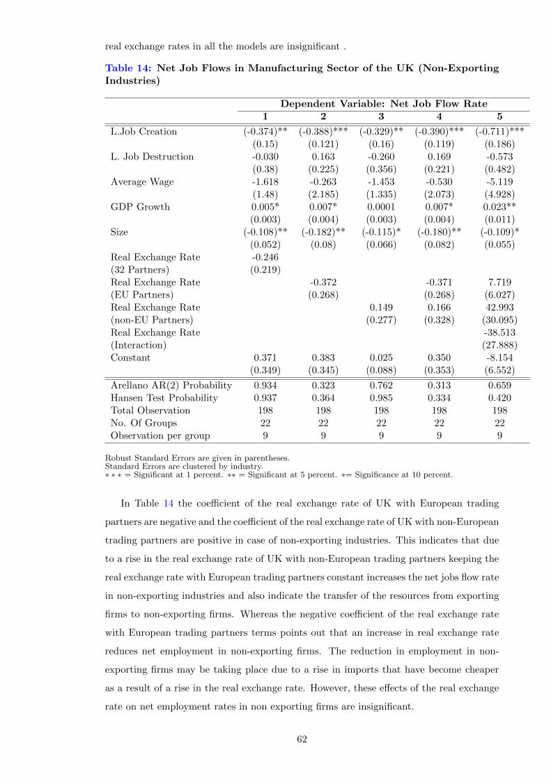
real exchange rates in all the models are insignificant .

Table 14: Net Job Flows in Manufacturing Sector of the UK (Non-ExportingIndustries)


L.Job Creation (-0.374)** (-0.388)*** (-0.329)** (-0.390)*** (-0.711)***(0.15) (0.121) (0.16) (0.119) (0.186)

L. Job Destruction -0.030 0.163 -0.260 0.169 -0.573(0.38) (0.225) (0.356) (0.221) (0.482)

Average Wage -1.618 -0.263 -1.453 -0.530 -5.119(1.48) (2.185) (1.335) (2.073) (4.928)

GDP Growth 0.005* 0.007* 0.0001 0.007* 0.023**(0.003) (0.004) (0.003) (0.004) (0.011)

Size (-0.108)** (-0.182)** (-0.115)* (-0.180)** (-0.109)*(0.052) (0.08) (0.066) (0.082) (0.055)

Real Exchange Rate -0.246(32 Partners) (0.219)Real Exchange Rate -0.372 -0.371 7.719(EU Partners) (0.268) (0.268) (6.027)Real Exchange Rate 0.149 0.166 42.993(non-EU Partners) (0.277) (0.328) (30.095)Real Exchange Rate -38.513(Interaction) (27.888)Constant 0.371 0.383 0.025 0.350 -8.154

(0.349) (0.345) (0.088) (0.353) (6.552)



In Table 14 the coefficient of the real exchange rate of UK with European trading

partners are negative and the coefficient of the real exchange rate of UK with non-European

trading partners are positive in case of non-exporting industries. This indicates that due

to a rise in the real exchange rate of UK with non-European trading partners keeping the

real exchange rate with European trading partners constant increases the net jobs flow rate

in non-exporting industries and also indicate the transfer of the resources from exporting

firms to non-exporting firms. Whereas the negative coefficient of the real exchange rate

with European trading partners terms points out that an increase in real exchange rate

reduces net employment in non-exporting firms. The reduction in employment in non-

exporting firms may be taking place due to a rise in imports that have become cheaper

as a result of a rise in the real exchange rate. However, these effects of the real exchange

rate on net employment rates in non exporting firms are insignificant.

62

We also find that in non-exporting firms the net job flows are mainly determined by

GDP growth. Columns 1, 2, 4, and 5 of Table 14 show that the coefficients on GDP

growth rates are positive and statistically significant. This implies that an increase in

GDP growth leads to a rise in employment in non-exporting firms. The marginal effect

of the GDP growth rate on net employment rate for exporting industries are

0.005, 0.007, 0.007 and 0.023 for models 1, 2, 3, 4 and 5 in Table 14. A one

percent change in GDP growth rate leads to less than one percent change

in the employment2. This implies that in a time of prosperity employment

rises and in bad times employment falls. This result also indicates that the

overall macroeconomic environment in the country affects job flows in non-

exporting firms of manufacturing sector of the UK. This result remains valid

for the entire set of models we have estimated except when we consider non-

European trading partners of the UK. This may be due to the fact that most

UK trade takes place with other European countries.

Columns 1, 2, 3, and 5 of Table 14 show that the size of a firm in an industry

has a negative effect on net employment rates in the non-exporting industries.

The marginal effects of the size of a firm in an industry on net employment

rates in non-exporting industries are -0.108, -0.182, -0.115, -0.180 and -0.109

for models 1, 2, 3, 4 and 5 respectively, in Table 14. This implies that as the

size of a firm in an industry increases the fluctuations in the net employment

decreases. However, our results indicate that one percent change in size of a

firm in an industry leads to a less than one percent change in the employment3.

Results shown in Table 14 implies that for non-exporting firms, the bigger the

firm, the lesser will be the net change in employment in response to a shock.

Net job flows decrease with the increase in the size of the firm. This indicates

that smaller firms are more vulnerable to a shock. In other words, we can

say that bigger firms have more capacity to bear shocks and the adjustment

in employment in bigger firms is relatively low. This result is very stable and

does not change with the change of specification.

We also find that a shock to the real exchange rate neither creates nor destroys jobs

in non-exporting industries. The coefficients of the real exchange rates in the entire set

of the models we have estimated for job creation and job destruction in non-exporting

industries are insignificant (see Tables A.4 and A.5 in Appendix A). This implies that job

creation and job destruction in non-exporting industries of the UK manufacturing sector

2The elasticities of net employment rates to GDP growth rates for these coefficients are -0.19, -0.26,-0.19, -0.004 and -0.87

3The elasticities of net employment rates to GDP growth rates for these coefficients are 0.34, 0.57, 0.36,0.57 and 0.34

63

are insensitive to variations in the real exchange rate. Once again our finding that changes

in real exchange rate do not bring changes in job creation or job destruction for non-trading

industries is consistent and does not vary with change to the model specification.

Table A.4 in Appendix A show previous period job creation rates, GDP growth and

average wages play a significant role in determining the job creations rates. The negative

and statistically coefficients of the previous period job creation rates and the average wages

indicate that other things remaining the same, a rise in previous period job creation rates,

and a rise in average wages decrease job creation rates significantly. Whereas positive and

statistically coefficients of the GDP growth rates indicate that a rise in GDP growth rates

increases the job creation rates in non-exporting industries significantly. The marginal

effect of the previous period job creation rates, average wages and GDP growth rates

are -0.110, -1.429 and .009 respectively when in the model 1. The marginal effects of

these variables are similar in other four model given in the Table A.4 in Appendix A. The

positive coefficients of GDP growth rate implies that other thing remaining the same, as

the GDP growth rate rise the firms increase hiring the new staff which leads to increase

in the opportunities to get employed for the existing unemployed workers and for the new

workers joining the labor force. The negative coefficients of average wages implies that

other thing remaining the same, as wages rise firms reduce hiring new staff which leads

to a reduction in the opportunities to get employed for the existing unemployed workers

and for new workers joining the labor force.

However, a one percent change in the previous period job creation rates, average wages

and GDP growth rates leads to less than one percent changes in job creation rates because

the elasticities in job creation rates with respect to previous period job creation rates,

average wages and GDP growth rates are less than one for all the models we have estimated

except for average wages in model 4 and for GDP growth in model 54. Whereas, Table

A.5 in Appendix A indicates that the job destruction rate is mainly determined by the

previous period job destruction rates and no other variable has a significant effect on

job destruction rates except GDP growth rates which is significant in model 5. Results

presented in Tables A.4 and A.5 in Appendix A show that GDP growth significantly

determines job creation and job destruction in non-exporting industries. However, GDP

growth affects job creation significantly in all five models, and job destruction in one out

of five models we have estimated. Therefore, we can say that our finding is consistent and

does not change with the change of model specification. In addition, we may say that the

4The elasticities of job creation rate with respect to previous period job creation rates are -0.12, -0.13,-0.10, -0.13 and -0.18 for models 1, 2, 3, 4 and 5 respectively. The elasticities of job creation rate withrespect to average wages are -0.61, -0.90, -0.58, -1.08 and -0.98 for models 1, 2, 3, 4 and 5 respectively.The elasticities of job creation rate with respect to GDP growth rates are 0.39, 0.56, 0.13, 0.52 and 1.82for models 1, 2, 3, 4 and 5 respectively.

64

adjustment process in net employment to a shock in average wages mainly works through

job creation because fluctuations in average wages affect job creation significantly and job

destruction insignificantly in most of the models we have estimated (see Tables A.4 and

A.5 in Appendix A).

With regard to firm-specific variables, we find that a rise in average wages does not

affect job destruction but significantly reduces job creation in non-exporting firms of the

UK manufacturing sector. This implies that non-exporting firms do not lay off their exist-

ing staff when they face higher wages. However, they avoid new recruitment when wages

rise. As a result, the effect of a rise in wages on net employment becomes insignificant

(see Table 14). Table A.6 in Appendix A shows that gross flows of the jobs are mainly

determined by previous period job creations and job destruction rates. Tables A.4 and

A.5 in Appendix A also support this observation. These two tables show that job creation

and job destruction rates are significantly determined by their lags.

Overall, our results show that a change in wage costs of the UK manufacturing sec-

tor relative to the wage costs in UK’s trading partners does not affect net employment

in non-exporting industries of the UK. Moreover, variations in the real exchange rates

neither create nor destroy jobs in non-exporting industries of the UK. Average wages and

GDP growth play a major role in explaining the dynamics of the employment in non-

exporting industries. Moreover, these results remain consistent whether we consider the

real exchange rate of the UK with 32 trading partners of the UK or we take into account

real exchange rate of the UK with only European or real exchange rate of the UK with

non-European trading partners of the UK only.

2.5 Conclusions

Shocks to the real exchange rate change incentives to produce tradable versus non-tradable

goods and generate labor market adjustment costs and may end up with net losses/gains

in employment. Along with the size of adjustment costs, how the adjustment process in

employment works is really important in labor market analysis. In this paper we have

analyzed three main questions. First, how employment in UK manufacturing responds

to a real exchange rate-led shock in competitiveness. Second, whether the adjustment in

employment works through job creation or job destruction. And third, whether the effect of

real exchange rate-led changes in UK competitiveness with European and non-European

countries is similar. Furthermore, the data we used provide us with an opportunity to

extend our analysis to exporting and non exporting firms of the UK manufacturing sector.

Using GMM we have estimated the dynamics of employment adjustments due to a

shock in competitiveness for the UK manufacturing sector. Our first conclusion is that

there is a significant reduction in the employment due to a rise in UK wage costs relative

65

to its trading partners. This effect is more pronounced in industries that export relatively

more. However, the effect is small economically.

Second, the adjustment in net employment to a shock in competitiveness is significantly

driven by job creation and not significantly affected by job destruction. However, in

job creation previous period job destruction plays a more important role. Our results

are comparable to the results of Moser et al. (2010) for Germany, Abowd et al. (1999),

Gourinchas (1999) for France who found that job creation is more sensitive to shocks to

the real exchange rate as compared to job destruction. However, Moser et al. (2010) found

lower coefficients as compared to those we reported here.

Moreover, our results suggest that the UK labor market responds to shocks and in-

duces the employment smoothing accordingly. For example, temporary shocks to GDP

significantly explain job creation, job destruction and net flows. This implies that workers

fired in bad times will be rehired in good times. So, employment will be high in good

times but low in bad times.

Similar to the Hijzen et al. (2010) findings regarding the contribution of smaller firms

to employment fluctuations, we also find that smaller firms contribute more towards job

creation and slightly less towards job destruction than larger firms. This implies that

employment in small firms is more sensitive to fluctuations in competitiveness than large

firms. Furthermore, the size of labor adjustment in the UK manufacturing sector in

response to real exchange rate led fluctuations in competitiveness of the UK with European

and non-European countries differs. This observation is similar to the results of Burgess

and Knetter (1998) that the size of labor adjustment in response to a shock in real exchange

rate varies from country to country.

Moreover, we found that fluctuations in real exchange rate may not affect net employ-

ment in non-exporting firms. However, the increases in real exchange rate significantly

reduce net employment in exporting firms. So we can say that employment in exporting

and in non-exporting firms behave differently in response to a change in the real exchange

rate. In fact, changes in the real exchange rate put more pressure on net employment

through job creation than job destruction in both exporting and non-exporting firms of

the manufacturing sector of the UK.

Finally, the average wage cost affects jobs creation significantly but does not foster job

destruction. This suggest that insiders benefit from higher wages while outsiders bear the

cost of the job reallocation process.

66

Chapter 3

Financial Turmoil, External Finance and UK Exports

3.1 Introduction

The funds that a firm acquires from the external resources such as banks

and other financial institutions to finance their productive activities are called

external finance. Availability and easier access to the funds from external resources

play an important role in growth and development of a country. The growing literature

in trade and finance establishes the fact that access to finance is a key ingredient in firms’

growth. According to the Business Environment and Enterprise Survey BEEPS (2010),

about 66% of the respondent firms in 29 countries of Europe and Central Asia (ECA) and

63% of EU-10 countries respondent firms report that access to external finance is one of the

major obstacles in doing business. Furthermore, this report indicates that the percentage

of firms indicating unfavorable interest rates as the main reason for not applying for a

loan ranges from about 2 to 42% of the firms surveyed. Overall, the survey suggests

that unavailability of external funds at affordable costs is a major obstacle in starting,

maintaining or extending business to foreign markets. In other words, credit constraints

may prevent firms from extending their business across borders.

Several empirical studies have examined the relationship between trade and finance

from different dimensions. Some of them look into the impact of financial development

on international trade and show that financial development promotes international trade.

For example, Beck (2003) finds that countries with better developed financial system have

higher export shares and trade balances in the industries that use more external finance.

Similarly, Hur et al. (2006), using cross-country industry level data, report that financial

development increases export shares and trade balances. On the other hand, some studies

have examined the linkages between access to external finance and cross border economic

activities. For instance, Berman and Hericourt (2010) using a large cross-country firm-

level data set of nine developing and emerging economies show that financial constraints

create a disconnection between a firm’s productivity and its export status. Manova et al.

(2011) using Chinese firms’ data show that credit constraints restrict international trade

flows. Specifically, their findings indicate that limited credit availability hinders firms’

trade flows.

Another dimension explored in the trade and finance literature is how credit constraints

affect firms’ decisions to enter in international markets. Minetti and Zhu (2011) find that

the probability of exporting in Italian credit-rationed firms is 39% lower and that credit

67

rationing reduces foreign sales by more than 38%. Similarly, using UK firm-level data,

Guariglia and Mateut (2010) study the links between firms’ global engagement status

and their financial health and show that the global engagement of firms improves their

financial health, suggesting that firms involvement in cross-border activity shields them

from financial constraints.

In general, researchers have established the fact that financial constraints reduce in-

ternational trade. However, empirical evidence on how firms exports respond to financial

constraints during the financial crisis is limited. According to my knowledge there is only

one paper by Chor and Manova (2011) which explores how international imports to the

USA reacted during the financial crisis. They show that countries with higher interbank

rates export less to the USA. They also show that this negative relationship has been

further intensified during the recent financial crisis when the interbank rate shot up. Fur-

thermore, they find that industries that require more external finance, with lower access

to trade credit and lower collateralizable assets, export less, and this effect becomes even

stronger during financial crisis. According to WTO (2010), the volume of the global trade

contracted by 12.2% during 2007-2009 global economic crisis. It was the largest decline in

world trade since World War 2.

Moreover, the intensity of the decline in trade flows caused by the financial constraints

seems to increase during the financial crisis (Chor and Manova, 2011). According to WEO

(2010) annualized quarter-over-quarter drop in the global real GDP averaged under 6%

from the last quarter of 2008 to the first quarter of 2009, whereas the drop in global real

imports was five times as large and averaged over 30% during the same time period. The

same source reports that volume of the global trade which was growing at 2.9% in 2008

showed a decrease of 11% in 2009. During this period the imports and exports of the

advanced economies declined more rapidly than the imports and exports of the emerging

and developing economies. The imports and exports of the advanced economies declined by

12.7% and 12.4% respectively in 2009, whereas the imports and exports of the emerging

and developing economies declined by 8.2% and 7.8% respectively in 2009. Similarly,

Mora and Powers (2009) report that nominal global merchandise exports dropped by 32%

between the second quarter of 2008 and second quarter of 2009.

Mora and Powers (2009) consider the decline in trade financing as a major contributor

towards the decline in the world trade during the second half of 2008 and early 2009. Sum-

marizing the findings of the 6 surveys of international banks, suppliers, and government

agencies, Mora and Powers (2009) point out that trade financing is number two cause of

the decline in the global trade after falling the international demand. In these surveys,

among international suppliers, 30 % consider reduced supply of trade financing as a key

factor in lowering foreign sales, and 57 % of the banks reported that lower credit availabil-

68

ity contributed to trade decline between the second half of 2008 and early 2009. Banks

reduced the supply of trade financing in last quarter of 2008 the trade financing and the

value of letters of credit fell by 11% in this quarter. Furthermore, the global impact of the

crisis on trade financing peaked in the first half of the 2009.

Similarly, quoting the surveys of International Monetary Fund (IMF) and the Bankers

Association for Finance and Trade (BAFT) now merged with International Financial Ser-

vices Association (BAFT-IFSA), Chauffour and Malouche (2011) report that about 40

percent of trade finance was bank intermediated whose prices increased considerably dur-

ing the 2007-2009 financial crisis. Mora and Powers (2009) report that the price of letter

of credit increased by 70 base points and the price of export credit insurance increased

by 100 base points during the crisis. The trade cost on average increased by about 11%

between the second quarter of 2008 to the first quarter of 2009 (Jacks et al., 2009). This

rise in the costs of the trade in general and the increase in the cost of trade finances in

particular played their role in the collapse of global trade. Thus, it appears that reduction

in the availability of the trade finance, and the rise in the cost of the trade finance resulted

in the fall of the global trade. So, it is worthwhile to analyze whether trade finance was

indeed a major factor driving the fall in UK trade during the recent financial crisis.

Thus, in this chapter we analyze how UK exports responded to external financing

during the financial crisis of 2007-2009. It is useful to analyze UK exports during the

financial crisis because the UK is the seventh largest producer of manufacturing goods

and the fifth largest exporter of manufacturing goods in the world (Garcia-Vega et al.,

2012). Furthermore, on average 30 percent of the total sales of UK manufacturing firms are

directed abroad. The UK is the second largest host to multinational enterprises (Guariglia

and Mateut, 2010). Moreover, UK is one of the economies that was severely affected by the

financial crisis 2007-2009. During the crisis, the UK’s growth rate fall to -0.4 percent (Das,

2010), unemployment rate increased to 7.8 percent and the lending interest rates shot up

to 6.5 percent per annum (Brancaccio and Fontana, 2010). Furthermore, in this crisis

the Northern Rock bank, Royal Bank of Scotland (RBS) and Halifax Bank of Scotland

(HBOS) got into trouble, RBS bank announced the loss of 24.1 billion pounds, the biggest

loss of the corporate history, and the share price index decreased to 83.59. The UK’s credit

market was dried up and credit provided to the private sector decreased to $3.353 billion.

Moreover, during the crisis period 25 percent of UK manufacturers reported lack of credit

as a major hurdle in fulfilling their export orders and 15 percent of manufacturers reported

lack of credit as a factor likely to constraint their investment in next twelve months (BOE,

2011). Furthermore, UK exports declined drastically during the crisis period; the details

of decline in exports are given in Table 16. In order to rescue the UK’s banks, Bank

of England slashed the interest rate to 0.5 percent and the UK government announced a

69

bailout package of £400 billion worth. The UK government measures to encourage lending

and to revive confidence in financial markets have increased UK taxpayer liability to 1.5

trillion pounds (Oxlade, 2012). These facts about the UK economy during the financial

crisis 2007-2009 raise the importance of the analysis which estimates the impact of the

financial crisis on UK sectoral exports. We use monthly UK exports data to estimate the

effects of the global financial crisis 2007-2009. Our sample period consists of January 2002

to September 2011.

We contribute to the existing literature in three aspects. First, the existing literature

estimates the impact of the current global financial crisis on US exports, whereas we focus

on UK exports. Second, in the previous literature researchers analyzed the impact of the

financial crisis on exports from the supply side only. Rather, we estimate the impact of

the financial crisis on exports considering both the demand and supply sides. Finally, we

use monthly data whereas most of the previous studies have used annual data.

We show that financial dependence is significant in determining the volume of UK

exports. Specifically, we find that the impact of financial dependence is negative and

statistically significant. We also show that the negative relationship between financial de-

pendence and the ability of firms to export became relatively stronger during the 2007-2009

financial crisis. These results hold when we use different proxies for financial dependence

in our analysis.

Further, our findings suggest that GDP and the capital-labor ratio of the UK and

the GDP and claims on the private sector of the importer country have positive and

significant impact on UK sectoral exports. Moreover, we found that the capital-labor

ratio and interest rates of importer countries are negative and statistically significant. We

also observe that the UK lending rate affects UK exports negatively.

In general, our findings remain unchanged when we use the overnight interbank rate

instead of the lending rate as a measure of cost of capital. They remain unchanged even

when we use an instrumental variable (IV) approach to estimate the model. Furthermore,

the negative impact of financial dependence on exports holds when we extend our analysis

to the sectoral level; we find that those sectors that rely more on external finance, have

lower access to trade credit and have lower collateralizable assets export less relatively.

The rest of the Chapter is organized as follows. Section 3.2 reviews the studies that

have focused on the effects of financial dependence on exports. A brief review of financial

crisis 2007-2009 is also presented in this section. Section 3.3 describes the data we use in

our empirical analysis and discusses the construction of the variables. Section 3.4 presents

the empirical model which we estimate in order to examine the impact of financial crisis

on UK sectoral exports. Section 3.5 presents and discusses the empirical findings. Finally,

Section 3.6 presents conclusions.

70


The linkages between trade and finance have been extensively analyzed both theoretically

and empirically. Researchers mainly focus on estimating the impact of overall financial

conditions in a country on international trade, in explaining the channels through which fi-

nancial constraints influence the cross-border flows of goods and services, and on exploring

whether firms’ participation in exporting activity affects their financial health. In general,

the trade and finance literature establishes the fact that financial constraints affect inter-

national trade. However, this effect varies across firms, industries, sectors and countries

depending on their dependence on external finance and overall financial conditions in the

country.

Several studies document that in the presence of credit constraints, countries with

more developed financial markets have a comparative advantage in financially vulnerable

sectors. Beck (2002), using 30 years data for 65 countries, explores the link between

financial development and trade in manufactures. He shows that countries with better-

developed financial sectors have a comparative advantage in manufacturing industries.

Moreover, he also shows that financial development has a significant impact on both the

level of exports and trade balance of manufactured goods. Similarly, Kletzer and Bardhan

(1987) show that a well-developed financial sector can theoretically lead to a comparative

advantage in industries that rely more on external financing. Hur et al. (2006) report a

positive relationship between financial development and industry-level exports. In short,

the development of the financial system in a country boosts exports by providing easy

access to financial resources to the exporters.

With regard to the association between firms’ financial health and their exporting

activities Greenaway et al. (2007), using data of UK manufacturing firms, show that

exporter firms exhibit better financial health than non-exporter firms. In fact, not only

does firms’ financial health affect exports but firm involvement in international trade also

affects firms’ financial status. Regarding the impact of firms’ participation in cross-border

sales on the financial health of firms, Greenaway et al. (2007) and Guariglia and Mateut

(2010) analyze the link between global engagement status and financial health of the

UK firms and find that global engagement status shields firms from financial constraints.

Hence, the existing literature seems to establish a two-way causality between financial

health and firms’ exporting status.

Evidence from existing studies suggests that trade finance is a key element in de-

termining the volume of international trade. According to Auboin (2009) 80 to 90% of

world trade depends on some form of trade financing. This implies that countries with

better financial markets have a comparative advantage in accessing foreign markets and

71

extending their business beyond their national borders because developed financial mar-

kets provide trade credits on easier terms and conditions than relatively less developed

financial markets.

In fact, trade financing generates funds to cover substantial upfront sunk costs that

firms intending to start exporting activity or to extend their business in global market

have to pay but cannot be financed with internal cash flows. This implies that policies

that ensure the availability of funds at easier terms and conditions will stimulate trade.

By and large, the trade and finance literature identifies three main reasons of exports’

reliance on external finance. First, firms have to bear additional upfront fixed sunk costs

as well as some variable costs specific to international trade which cannot be met from

internal cash flows. Sunk costs include expenditures made to search for profitable export

markets and to set up marketing and distribution networks abroad. They also include

outlays incurred in adapting the product to meet international standards and regulatory

compliance and variable costs consisting of expenditure on shipping and customs duties.

In most cases firms have to bear these expense before the export revenues are realized.

In order to finance these expenditures, exporters opt for external resources. Second, on

average international transactions take 30 to 90 days longer than domestic transactions

which further intensifies an exporter’s need for external capital (Chor and Manova, 2011).

Finally, cross border business activities involve more risk relative to domestic business

activities. To avoid this risk exporters have to insure their transactions for which they

have to pay insurance premium leading to an increase in the cost of exporting and further

intensifying the need for external capital. As a result of the risks associated with trade,

the benefits/profit of trade may fall.

Although sunk entry cost is crucial for exporters, it varies with the size of firms. Das

et al. (2007) show that on average sunk entry cost for Colombian small producers is higher

and ranges from 430,000 to 412,000 US dollars while for large producers on average it is

lower and ranges from 334,000 to 402,000 US dollars. However, they report similar sunk

entry costs across sectors. In sum, in the presence of a sunk entry cost, exporting becomes

a challenge for firms. Furthermore, firms have to bear these costs before they actually

start exporting their product. This implies that only firms with sufficient liquidity can

expand their business beyond national borders.

The above mentioned factors indicate the significance of financial markets for cross-

border trade. Any disruption in financial markets which constrained the liquidity available

may affect firms’ decisions to sell their products in global markets and affects the overall

volume of trade. Recently, using Italian firm level data, Minetti and Zhu (2011) show that

credit constraints impede exporting activities of firms. This negative impact of credit con-

straints on exports becomes stronger during the financial crisis when the supply of funds

72

becomes worse. Likewise, Auboin (2009) reports that 10-15% of the fall in international

trade in the second half of 2008 was due to a fall in the supply of trade finance. Further-

more, the size of global market for trade finance in 2008 is estimated at the $10-12 trillion,

which is almost 80% of the total value of world trade in 2008. In a nutshell, international

trade and finance are closely linked and among others factors global trade also reflects

variations in financial markets.

Thus, researchers working on trade and finance use different firm-specific variables to

denote firms’ dependence on external resources and to evaluate the impact of external

financing on international trade. For instance, to reflect firms’ requirement for outside

capital Rajan and Zingales (1998) and Chor and Manova (2011) use the fraction of total

capital not financed by internal cash flows. This measure of firms’ financial dependence

along with reflecting the volume of formal trade financing also indicates firms’ long term

need for external capital. Using this definition of firms’ dependence on external finance

to estimate the impact of external finance on exports Chor and Manova (2011) show that

countries with high costs of capital export less in sectors that depend more on external

resources.

Buyer-supplier trade credit is another important indicator which shows firms’ depen-

dency on external finance and reflects short term working capital needs of firms and affects

cross border trade. Petersen and Rajan (1997), Fisman and Love (2003) and Chor and

Manova (2011) use buyer-supplier trade credit as a potential substitute for formal trade

financing. Their findings indicate that firms with greater access to buyer-supplier trade

credit export more relative to firms with lower access to buyer-supplier trade credit. Fur-

thermore, Brennan et al. (1988) and Long et al. (1993) argue that buyer-supplier trade

credit is used to ensure the quality of the product and as an incentive to discriminate

among cash and credit customers. Since buyer-supplier trade credit does not come from

formal banking channels, firms with a greater access to buyer-supplier trade credit may

show some resilience to the detrimental effects of a financial crisis which squeezes liquidity

and makes it harder for firms to get credit from formal banking channels.

Along with the availability of external funds, the ability of firms to acquire these

funds also matters. Therefore, firms’ endowment of tangible assets which determines their

ability to acquire funds from formal banking channels becomes important. In principle,

firms characterized with more tangible assets can offer greater collateral to acquire external

funds. Researchers use tangible assets as an inverse proxy for the financial vulnerability

of firms. For example, Chor and Manova (2011) use tangible assets as an inverse proxy for

the financial vulnerability of sectors to estimate the impact of the financial crisis on US

imports. Their findings show that the exports of the sectors with higher endowments of

tangible assets are less sensitive to adverse credit conditions during the 2007-2009 financial

73

crisis.

So far we have discussed studies which focus on the overall impact of financial devel-

opment on international trade. Now we emphasize how international trade behaves in

response to unexpected events happening in financial markets which reduce the availabil-

ity of funds. In fact, the importance of financial resources in promoting and extending

cross border trade flows magnifies when financial markets face a liquidity crunch and trade

financing dries up. Indeed, financial crisis depletes trade financing and creates a gap be-

tween demand for and supply of trade finance. Chauffour and Malouche (2011) report

that the gap between demand and supply of trade finance in US financial markets was

estimated at around $25 billion during the 2007-2009 financial crisis. Furthermore, they

report that this gap increased to around $300 billion in secondary markets with the spread

of financial crisis from USA to EU and then to the developing countries. This suggests

that the trade finance market dried up globally during the 2007-2009 financial crisis.

Consequently, firms became financially constrained and their output, employment and

sales declined in both domestic and foreign markets. In particular, foreign sales contracted

drastically during the financial crisis. Levchenko et al. (2011) report that from the second

quarter of 2008 to second quarter 2009 US imports declined by 21.4 percent and exports

dropped by 18.9 percent. Similarly, Auboin (2009) reports that 10-15% of the fall in

cross border trade in the second half of 2008 was caused by the fall in the supply of trade

finance. In the same vein Amiti and Weinstein (2011) estimate that the 1997 banking crisis

caused a 10.5 percent decline in Japanese exports. Bricongne et al. (2012) report similar

results for French sector level exports. In short, financial crisis has severe consequences

for international trade.

However, the financial turmoil’s effect on cross border trade varies from firm to firm,

industry to industry, sector to sector and from country to country depending on the size

and dependency of firm, industry or sector on external financial resources and on the level

of financial markets developments in the country. For instance, Chor and Manova (2011)

report that credit constraints hinder international trade and this hindrance intensified

during the 2007-2009 financial crisis when acute shortage of trade financing prevailed in

the financial markets. Moreover, they find that exports decreased relatively more in sectors

which rely more on external finance, have limited access to buyer-supplier trade credit and

have fewer collateralizable assets.

On the whole, the existing literature establishes a strong link between external finance

and international trade flows. Specifically, researchers consider that credit constraints

hinder cross border flows of goods and services. However, the literature on how interna-

tional trade flows respond to unexpected events like liquidity crisis in financial markets

is limited. Existing work mainly focuses on USA and European countries. Particularly,

74

very few studies exist with reference to the impact of the 2007-2009 financial crisis on in-

ternational trade. Specifically, with reference to the response of international trade flows

of the UK during the 2007-2009 liquidity crunch the existing literature is scarce. Thus, to

look into effects of financial crisis on UK trade flows has worth and will contribute to the

trade-finance literature considerably.

3.3 A Brief Review of Financial Crisis 2007-2009

Financial crisis, or credit crunch, is not a new phenomenon. Financial markets in the

world have gone through sudden liquidity crunches in the past as well. According to Bordo

(2008) financial crises are as old as financial markets. However, the 2007-2009 financial

crisis differs from previous crises in its nature, intensity and in the level of damage to

economies facing the crisis.

The 2007-2009 financial crisis was a global crisis which started in the USA and spread

like a wild fire to other parts of the globe through asset markets, international banking and

through monetary standards. For instance, Das (2010) states that given the economic,

financial and trade inter-linkages of the world economy, the US financial crisis shifted to

other economies very quickly. Furthermore, during the crisis, valuation of the banks fell

and stock markets crashed across the countries. For example US and UK indices dropped

by more than three-quarters of their original value during this period (Wisniewski and

Lambe, 2011). As a result, many banks across the globe suspended their normal activities

and failed to honor their obligations. Specifically, Lehman Brothers, Bear Stearns, BNP

Paribas, Sachsen LB and Northern Rock bank were among the victims of the crisis.

In terms of intensity and damage, the 2007-2009 financial crisis was so damaging

that COP (2009) and De Larosiere (2009) described it as the worst crisis since the Wall

Street Crash and the Great Depression of late 1920s and 1930s. Likewise, Turner (2009)

considered it as the greatest crisis in the history of finance capitalism. Consequently,

economies facing the crisis were damaged intensively. For instance, the WorldBank (2011)

shows that growth rate of the world economy declined to -2.05 percent in 2009 from 3.94

percent in 2007. Similarly, high income economies, OECD, EURO Area, Japan and United

States declined to -3.53, -3.69, -4.18, -6.29 and -2.67 percent in 2009 which were growing

at 2.65, 2.54, 2.82, 2.36 and 1.94 percent, respectively, in 2007. However, low and middle

income economies showed a positive growth rate in 2009 and were growing at the rate of

2.78 percent in 2009. This suggests that financial crisis led to severe economic contraction

in advanced economies where financial markets are well developed.

Indeed, liquidity constraints arising from the financial crisis 2007-2009 have contributed

to falls in aggregate supply and demand. Output and employment decreased drastically

during the crisis period. For example, Das (2010) reports that the growth rate of the

75

second largest economy in Europe, i.e., the UK fell to -0.4 percent in third quarter of

2009. Similarly, Brancaccio and Fontana (2010) reports that the unemployment rate in

US rose from 4.7 percent in the fourth quarter of 2007 to 9.2 percent in the second quarter

of 2009. Likewise, unemployment in the UK moved from 5.1 percent to 7.8 percent, France

from 7.5 percent to 9.1 percent, Spain from 8.6 percent to 17.9 percent, and Ireland from

4.6 percent to 12 percent during the same time period. These examples of a decline in

growth rate and in employment indicate that the 2007-2009 financial crisis has affected

real sector intensively.

With regard to the reasons behind the financial crisis of 2007-2009, Brancaccio and

Fontana (2010) point to two issues. First, they argued that misguided underpricing of

the risk which made financial investors overconfident in measuring and managing the risk

lead to financial crisis. Second, they consider the ‘Greenspan Put’, i.e., loose monetary

policy of early 2000 as a major cause of the recent financial crisis. In a similar vein Bordo

(2008) suggests that major changes in regulations, lax regulatory oversight, a relaxation

of normal prudent lending and period of abnormally low interest rates contributed to the

crisis. Along with the default of subprime mortgage, the above mentioned factors created

uncertainty in financial markets about the soundness of loans for buyouts leading to drying

up the interbank lending market. The prevailing uncertainty and lack of funds available

in financial markets turned into a severe liquidity crisis in a very short period of time and

spread across the globe through trade and financial markets linkages.

Consequently, the governments and the central banks of some economies, plagued

with liquidity crisis, stepped in with fiscal and monetary stimulus to combat the crisis.

For example, in the case of monetary measures to combat crisis and to encourage lending,

the Bank of England slashed bank rate form 5% in 2008 to 0.5% in 2009 and the US

central bank kept bank rates close to zero in 2008. With reference to fiscal stimulus

Das (2010) reports that initially the US government provided a small stimulus worth

$152 billion in 2008 and later in 2009 president Obama signed a package worth $787

billion to save the banks. Furthermore, to rescue US financial institutions and to reduce

market rates the Federal Bank committed itself to purchase $1.7 trillion worth of treasury

bonds, mortgage-backed securities and agency debts. Similar measures were taken to save

the financial institutions of the UK. The BBC reports that in October 2008, the UK

government announced a $88 billion rescue package for the banking system. Moreover,

the UK government offered up to $350 billion in short-term lending support5.

In the context of the chronology of the events which took place during the 2007-2009

financial crisis, Wisniewski and Lambe (2011) and Brunnermeier (2009) state that early

signs of the crisis became visible in February 2007 when delinquency rates among subprime

5See, http://news.bbc.co.uk/1/hi/7521250.stm.

76

borrowers increased. Later, in June 2007, the leading investment bank Bear Stearns came

under pressure when two of its hedge funds failed to meet their margin calls. The crisis

intensified and spread to other economies with the passage of time. As Edmonds et al.

(2010) report the disruption in the banking operation intensified in August 2007 when

BNP Paribas suspended normal activities on three of its hedge funds and the ECB was

forced to provide liquidity, and the German Bank Sachsen LB became a victim of the

crisis. Failure of the banks to continue their normal activities generated chaos and a fear

of liquidity problem in the financial markets.

The fear of liquidity problems worsened with the collapse of Bear Stearns in March

2008. However, the financial crisis reached on its peak in September 2008 when Lehman

Brothers collapsed (Oxlade, 2012)6, followed by the announcements of bailout packages

for the banks by governments of the affected economies and mergers of banks in October

2008. Consequently, the public debts mounted up and macroeconomic conditions wors-

ened. Despite granting the generous bail out packages to banks by the government to

cope with the liquidity crisis, confidence in financial markets only slowly returned in April

2009.

Up till now we discussed the overall development of the crisis. Now we look into the

insights of the crisis with reference to the UK. The UK is one of the economies which has

been severely affected by the financial crisis of 2007-2009. The tidal wave of the crisis

starting with the repayment of the subprime mortgage in August 2007 entangled the UK

as well. At the same time, British house prices started to fall and triggered the financial

crisis in the UK. However, British house prices stabilized in April 20097. The overnight

interbank rate started to shoot up and reached to 6.5 percent per annum

in September 2008 which was 5.31 percent per annum in January 2007 and

share price index number decreased to 83.596 in October 2008 from 131.015

in June 2007, as a result the credit market dried. The claims on private sec-

tor which shows credit provided to private sectors decreased to $3.353 billion

in June 2008 from $14.082 billion in June 2007. This created distress in the

stock markets and share prices declined. The share price index dropped from

132.5 in May 2007 to 82.2 in November 2008 and declined further to 74.2 in

February 2009. As a result investment, output and exports declined. The

real exports of the UK declined to £4155.988 million in September 2008 from

£10025.571 million in July 2007 when the crisis started8. According HM Trea-

6Oxlade, A. (2012), Economy watch: Is the British economy already back into recession?http://9dj1o x.0.u.is/money/news/article-1616085/Economy-watch-What-Britain.html.

7See footnote 2 for reference.8These figures are taken from International Financial Statistics(IFS) 2011 data base.

77

sury’s Management Report (2012)9, following a news report leaked by BBC

that Northern Rock bank had approached the Bank of England for liquidity

support, on 14 September 2007 about £4.6 billion were withdrawn from the

Northern Rock bank. Furthermore, the report states that in January 2008

Royal Bank of Scotland (RBS) announced the biggest loss in the corporate

history, a loss of £24.1 billion. BOE (2011) reports that in 2007 less than 3%

of the UK manufacturers cited the lack of credit as a factor likely to constraint

their export orders over next three months, this number increased to 15% in

2009. In addition, in 2007, less than 2% of the UK manufacturers cited the lack

of credit as a factor likely to constraint their output over next three months,

this number increased to 25% in 2009. Consequently, UK exports declined.

However, the decline in exports varied from sector to sector.

For example, from October 2008 to November 2008 within the period of

one month Food and live animal exports dropped by 9.2 percent, Beverage and

tobacco exports decreased by 19.4 percent, Crude materials, inedible except

fuel exports decreased by 44.5 percent, Chemical and related products exports

dropped by 22.1 percent, Manufactured goods classified chiefly by material

decreased by 14.9 percent and Machinery and transport equipment exports

decreased by 11.9 percent. Similar trends were observed in the exports of

other commodities during this period (see Table 16 for details). These figures

show that the financial crisis 2007-2009 has affected the real economy of the

UK particularly the financial crisis 2007-2009 had severe consequences for the

UK exports.

In the chronology of events which took place in the UK during the financial crisis,

Northern Rock got into trouble and applied for liquidity support from the Bank of Eng-

land in September 2007 and finally was nationalized in February 2008 after two unsuc-

cessful bids. Similarly, in early October 2008 Halifax Bank of Scotland (HBOS) ran into

a trouble and through a bailout package was merged into Lloyds bank in January 2009.

On 8th October 2008 UK government announced 400 billion pound worth rescue plan for

the banks and nationalized HBOS and RBS, two largest banks of the UK and took the

partial ownership of the Lloyd TSB bank. According to Oxlade (2012) UK government

measures to encourage lending and to revive confidence in financial markets has increased

UK taxpayers’ liability to 1.5 trillion pounds.

In sum, the 2007-2009 financial crisis was global in nature and severely affected macroe-

conomic conditions across the globe. Indeed, acute liquidity constraints in financial mar-

9 Review of HM Treasury’s management response to the financial crisis, March 2012 Report availableat http://www.hm-treasury.gov.uk/d/review fincrisis response 290312.pdf

78

kets during the crisis have led to the contraction of the real sector in all the affected

economies. Thus, given the above mentioned facts it is important o investigate the impact

of 2007-2009 financial crisis on UK exports.



Given the state of the literature we use the models given in equations 3.4.1 and 3.4.2 to

analyze the impact of 2007-2009 financial crisis on the UK exports. These models are

modified versions of the model used by Chor and Manova (2011) to estimate the impact

of financial crisis on US imports. In their model, Chor and Manova (2011) consider only

demand side of the exports which is affected by changes in cost of the capital. Chor and

Manova (2011) interacted exporter country’s cost of capital with the financial

vulnerability of different sectors of the importing country. This implies that

Chor and Manova (2011) are changing the exporter country’s cost of capital

and observing its impact on exports through changes in the financial vulnera-

bilities of the sectors operating in the importing countries in response to the

changes in exporter country’s cost of capital. This may be incorrect because

fluctuations in the exporter country’s cost of the capital will affect the finan-

cial vulnerabilities of firms or the sectors operating in an exporting country

rather than affecting the financial vulnerabilities of the firms or the sector

operating in the importing country. Moreover, from the model proposed by

Chor and Manova (2011), we cannot differentiate whether fluctuations in the

cost of capital affect exports by affecting the demand for exports or by affect-

ing the supply of exports because Chor and Manova (2011) have interacted

exporter country’s cost of the capital with the financial vulnerability of the

sectors operating in the importing countries to measure the impact of the

financial vulnerability of the sector on exports.

Thus, to overcome the above mentioned problems in Chor and Manova

(2011) model we have modified it. In the modified model we interact exporter

country’s cost of the capital with financial vulnerability of firms or sectors

operating in the exporting countries to estimate the impact of the financial

vulnerability of a firm or a sector on its exports. This will give the impact of the

financial conditions in the exporting country on the supply of the exports. In

addition, we interact the cost of capital in the importer country with financial

vulnerability of firms or sectors operating in the importing country. This

will give the impact of the financial conditions prevailing in the importing

country on the demand for exports. So, from the modified model we can

79

easily bifurcate the impact of the variations in the cost of the capital on the

supply of exports and on the demand for exports.

The modified version of the model is given below in equations 3.4.1 and 3.4.2.

Exportsuk,kit = β1IBrateuk,t × EXTFINuk,k + β2DCrisis × IBrateuk,t × EXTFINuk,k

+ β3IBrateit × EXTFINi,k + Σnj=1αjZj +Dkt +Dit +Dik + εikt (3.4.1)

Exportsuk,kit = β0Exportsuk,kit−1 + β1IBrateuk,t × EXTFINuk,k

+ β2DCrisis × IBrateuk,t × EXTFINuk,k + β3IBrateit × EXTFINi,k

+ Σnj=1αjZj +Dkt +Dit +Dik + εikt (3.4.2)

where k = sector, t = time and i = importer country

Exportsuk,kit=UK exports in sector K going to importing country i.

IBrateuk,t=cost of capital in UK at time t. In principle, insurance costs and interest rates

charged on the exports credit lines would be the ideal measures to represent the cost of the

trade financing for the UK. However, unfortunately, a direct measure of insurance costs

and the rates charged on the exports credit lines are not available for the UK and for the

trading partners of the UK from the data sources we have used to get the data for this

chapter. Therefore, following Chor and Manova (2011) we use interbank lending rate as

a measure of cost of the capital or as a proxy for the trade financing in the UK and in

trading partners of the UK.

IBratei,t=cost of capital the cost of trade financing in importing country at time t. We

use the interbank lending rate as a measure of cost of the capital as a proxy for the trade

financing in trading partners of the UK.

EXTFINuk,k=dependence of sector k of the UK on external resources. We have used

four proxies; External Finance, Trade Credit, Tangible Assets and Leverage, to measure

the dependence of a sector k of the UK on external resources and their definitions are

given in the variable construction section.

EXTFINi,k=dependence of sector k of the importing country on external resources. We

have used credit to the private sector as a proxy to measure the dependence of sector k of

the importing country on external resources.

Z=is a vector of control variables and includes GDP of the UK, interest rates of the UK,

Capital labor ratio of the UK, importer country’s GDP, Capital labor ratio, interest rates,

and Time required to enforce a contract (TREC). All these variables directly or indirectly

affect UK exports and have been used as control variables in the literature. Note that in

80

our analysis exports, GDP of the UK, Capital-labor ratio of the UK, importer country’s

GDP, Capital-labor ratio are in log form.

Dit= Country-time fixed effects. They will capture the impact of the shocks to aggregate

production and bilateral exchange rates fluctuations in each importing country on their

imports over time.

Dkt= Sector-time fixed effects. They will capture the impact of the shocks to aggregate

production, bilateral exchange rates fluctuations on different sectors which vary across the

sectors depending on the size, vulnerability and trade volumes of a sector.

Dik= Country-sector fixed effects. They will capture the time-invariant sources of the

comparative advantage that affect the average pattern of the country imports across the

sectors.

DCrisis=dummy variable, equal to 1 if the period is crisis period, otherwise

zero. In our analysis, following (Wisniewski and Lambe, 2011) we use the

time period from May 2007 to February 2009 as the crisis period.

εikt= error term

In both models we use double interaction (IBrateuk,t × EXTFINuk,k) and

triple interaction (DCrisis × IBrateuk,t × EXTFINuk,k) terms. Here, the double

interaction term IBrateuk,t × EXTFINuk,k measures the sensitivity of financial

vulnerability of the sector k in the UK to fluctuations in the cost of capital.

IBratei,t ×EXTFINi,k measures the sensitivity of the financial vulnerability of

the sector k in the importing country to changes in the cost of capital. When

the cost of capital rises it becomes harder for a firm to acquire external fi-

nance leading to a reduction in output and exports especially in firms with

greater requirements for external finance. So, we expect the coefficient of

the IBrateuk,t × EXTFINuk,k term, i.e., β1 < 0. Similarly, the double interac-

tion term IBratei,t × EXTFINi,k measures the sensitivity of financial vulner-

ability of the sector k in importing country i to fluctuations in the interest

rates. The double interaction term IBratei,t × EXTFINi,k also measures fluc-

tuations in demand for imports of country i from the UK. So, the coefficient

of IBratei,t × EXTFINi,k term, i.e. β3 shows the sensitivity of UK exports to

changes in interest rates in importing country. As the cost of borrowing for

consumption purposes increases demand for imported goods decreases. Thus,

as a consequence, when the cost of borrowing increases it will decrease UK

exports as well. So, we expect the coefficient of the IBratei,t×EXTFINi,k term,

i.e., β3 < 0.

The triple interaction term DCrisis × IBrateuk,t × EXTFINuk,k measures the

sensitivity of financial vulnerability of the sector k in the UK to fluctuations

81

in the cost of capital during the crisis period. In fact, credit conditions in a

country become worse as the interest rate shoots up during the financial crisis

and in turn the cost of capital becomes very high. Subsequently, firms cannot

afford to raise external funds at high interest rates and cut down their output

and employment during periods of liquidity crunch. Consequently, domestic

and foreign sales decline. In particular, financially constrained firms’ exports

decline relatively more as compared to less constrained firms. Therefore, we

expect coefficient of the DCrisis × IBrateuk,t × EXTFINuk,k term, i.e., β2 < 0 as

well. In other words, we expect that the negative effect of a rise in interest

rate on exports intensifies during the credit crunch.

3.4.2 Construction of Variables

The funds that a firm acquires from the external resources such as banks

and other financial institutions to finance their productive activities are called

external finance. For firms’ dependence on external resources, we use the following four

proxies.

3.4.3 External Finance (EXTFIN)

External Finance (EXTFIN) is defined as the fraction of total capital expenditure not

financed by internal cash flows from operation (Rajan and Zingales, 1998):

EXTFIN =Total Capital Expenditure not Financed by Internal Cash Flows from Operation

Investment

It indicates firms’ long term need for external finance. A rise in interest rates makes

it costly for firms to get finance from formal banking channels and ultimately leads to a

decrease in cross-border activities of financially constrained firms. Therefore, we expect

the coefficients of IBrateuk,t × EXTFINuk,k and DCrisis × IBrateuk,t × EXTFINuk,k

terms, i.e., both β1 and β2 to be less than zero when using EXTFIN as a proxy for financial

dependence of the sector to estimate equation 3.4.1.

3.4.4 Trade Credit (TCRED)

Trade Credit (TCRED) is defined as the ratio of trade credit to the book value of total

assets of firms.

TCRED =Trade Credit

Book Value of Total Assets of Firm

This variable indicates firms’ short term working capital requirements (Chor and

Manova, 2011). Firms use trade credit as an alternative to borrowing from formal bank-

ing channels. Moreover, firms with a greater access to trade credit are less sensitive to a

82

rise in interest rates because they can finance their cross-border activities by using buyer-

supplier trade credit. Therefore, we expect the coefficients of IBrateuk,t × TCREDuk,k

and DCrisis×IBrateuk,t×TCREDuk,k terms, i.e., β1 and β2 to be greater than zero when

instead of EXTFIN we use TCRED as a proxy for financial dependence of the sector to

estimate equation 3.4.1. Furthermore, β2 can be less than zero as well if the crisis exhausts

the credit availability along with the other forms of financing to the firms to support their

exports.

3.4.5 Tangible Assets (TANG)

Tangible Assets (TANG) is defined as the ratio of tangible assets to book value of total

assets.

TANG =Total Tangible Assets


This proxy captures firms’ ability to pledge collateral in acquiring external borrowing

(Braun (2003) ; Claessens and Laeven (2003) ; Chor and Manova (2011)). Firms with

greater tangible assets can get funds from banks more easily because they can offer more

assets as collateral. Therefore, we expect the coefficients of IBrateuk,t × TANGuk,k and

DCrisis× IBrateuk,t×TANGuk,k terms, i.e., both β1 and β2 to be greater than zero when

instead of EXTFIN we use TANG as a proxy for financial dependence of the sector to

estimate equation 3.4.1.

3.4.6 Leverage (LEVERAGE)

Leverage is defined as the ratio of total debt to book value of total assets.

LEVERAGE =Total Debt


Leverage shows the riskiness of firms. Risks of default increase with an increase in

the leverage of firms. Banks try to avoid lending funds to firms with high leverage or

may lend to them at an interest rate which is higher than the interest rate which banks

charge firms with lower values of leverage. So, firms with high leverage may not be able to

get funds from banks easily and reduce their cross-border activities. Thus, we expect the

coefficients of IBrateuk,t×LEV ERAGEuk,k and DCrisis×IBrateuk,t×LEV ERAGEuk,kterms, i.e., both β1 and β2 to be less than zero when we use LEVERAGE as a proxy

for financial dependence of the sector to estimate equation 3.4.1. On the other hand, the

leveraged firms are normally big in their sizes, and can manage to get loans from the banks

to finance their production activities fulfill their export orders even under the financial

crisis situations. Thus, in this case the coefficients of IBrateuk,t × LEV ERAGEuk,k and

83

DCrisis×IBrateuk,t×LEV ERAGEuk,k terms, i.e., both β1 and β2 to be greater than zero

when we use LEVERAGE as a proxy for financial dependence of the sector to estimate

equation 3.4.1. If the crisis become so worse that the leveraged firms could not exploit

the banks to get the funds then the coefficient of DCrisis× IBrateuk,t×LEV ERAGEuk,kterms will be less than zero.

Note that we calculate these proxies at the firm level and then to match with sector

level data we take a median of all the firms operating in a sector.

3.4.7 Data Sources

The data we use for this study are taken from various sources and our sample period

consists of January 2002 to September 2011. Monthly data of UK exports are taken from

Overseas Trade Statistics, HM Revenue & Customs (HMRC). Overseas Trade Statistics,

HM Revenue & Customs (HMRC) provide detailed data on monthly exports and imports

of the UK. Furthermore, HMRC provides the break down on import and export data for the

UK according to regions, trading partners and Standard International Trade Classification

(SITC) commodity codes. Note that our sample covers UK exports going to 25 major

trading partners only. Table 9 shows these trading partners. Also note that these trading

partners account for more than 80% of UK exports. Thus, the selection of the sample

seems reasonable.

Table 15: The UK Major Trading Partner

No Trading partner No Trading Partner

1 BELGIUM 14 NETHERLANDS2 CANADA 15 NORWAY3 CHINA 16 POLAND4 CZECH REPUBLIC 17 QATAR5 DENMARK 18 RUSSIA6 FRANCE 19 SINGAPORE7 GERMANY 20 SPAIN8 HONG KONG 21 SWEDEN9 HUNGARY 22 SWITZERLAND10 INDIA 23 TAIWAN11 IRISH REPUBLIC 24 TURKEY12 ITALY 25 USA13 JAPAN

In order to measure the financial dependence of the sectors, firm level data are taken

from Financial Analysis Made Easy (FAME). FAME provides detailed information on

companies for a period of ten years. Moreover, the majority of the firms, for which FAME

provides data, are not listed on the stock exchange. In general, non-listed companies are

small, financially constrained, possess lower assets and have poor credit ratings as com-

84

pared to large, financially sound, and well-established listed companies with better credit

ratings. In addition, smaller firms are likely to face more problems in obtaining financial

resources from banking and non banking channels relative to the large firms. Thus, our

proxies for the financial dependence of firms should provide a good representation of fi-

nancially constrained firms. Table B.5 provides the characteristics of the sectors and the

number of firms included in each sector included in our sample. Monthly lending interest

rate, overnight interbank rate, consumer price index and claims on private sector of part-

ner countries and of the UK, are extracted from International Financial Statistics (IFS).

Data of the UK’s GDP,labor force and gross fixed capital formation and the GDP, labor

force, gross fixed capital formation and the time required to enforce a contract (TREC)

of partner country are extracted from the World Development Indicators (WDI).

3.4.8 At First Glance

Table B.4 given in Appendix B reports the means, standard deviations, maximum and

minimum values of the key variables used in the analysis, before, after and during the

financial crisis 2007-2009. This table shows that on average the lending rates and overnight

interbank rates have increased on average during the financial crisis which indicate that

the credit markets of the UK were tighten and the credit availability to firms to finance

their production activities to fulfill their export orders have lowered during the crisis.

Table B.4 given in Appendix B also indicates that on average the cost of capital increased

during the financial crisis and has played its role in decreasing UK exports. This decline

in the UK exports is shown in Table 16. Table 16 shows that if we compare total exports

at the start of the crisis and the exports when recovery started the total exports of the UK

have declined by 13.8 percent. Furthermore, Table 16 shows that total exports declined

by 14.2 percent within the period of one month, from October 2008 to November 2008,

when the crisis was at its peak.

Our objective is to explore how the financial crisis of 2007-2009 has affected

the UK exports. To achieve this goal we a require measure of credit conditions

in the UK and in trading partners of the UK as our key explanatory variables.

The interest rates charged on export credit lines or insurance would be the

ideal variables to be used as a direct measure of the cost of trade financing.

But unfortunately, the data of the rates charged on export credit lines or in-

surance is not readily available for the countries included in our sample from

the data sources that we have used for this chapter. Therefore, following Chor

and Manova (2011) we use interbank lending rates as a proxy to measure the

cost of trade financing. Chor and Manova (2011) state that in the absence of

systematic information on the cost of trade financing, the interbank lending

85

Table 16: Percentage Decline in the UK Exports at the Peak and During theFinancial Crisis

Sector Peak of Overallthe Crisis during the Crisis

Food and Live Animal -9.2 11.1Beverages and Tobacco -19.4 -7.7Crude Materials, Inedible except Fuel -44.5 -32.7Minerals Fuels, Lubricants and Related material -11.5 -5.5Animal and vegetable oils, Fats and Waxes -9.9 47.6Chemical and Related Products, n.e.s -22.1 5.9Manufactured goods classified chiefly by material -14.9 -38.8Machinery and Transport Equipments -11.9 -24.9Miscellaneous manufactured article -9.0 -11.7Commodities and Transactions not Classified elsewhere in the SITC -10.6 8.7

Total Exports -14.2 -13.8Note: Calculated from Overseas Trade Statistics, HM Revenue & Customs (HMRC) monthly data on UKexports. Peak of the Crisis values are calculated using the exports from October 2008 to November 2008.Overall during the Crisis values are calculated using the exports from March 2007 to February 2009.

rate can serve as a broader measure of the cost of external finance in the econ-

omy and also as a proxy for the cost of trade financing. Basically, interbank

rate is an interest rate that commercial banks charge from each other for a

short term loan which a commercial bank acquires from the other commer-

cial banks to adjust liquidity positions and to meet the reserve requirements.

Furthermore, the interbank lending rate serves as a benchmark for the overall

cost of the credit in the economy and other interest rates such as a mortgage

rates and commercial banks lending rates take a clue from it. However, Chor

and Manova (2011) state that the interbank rate is a noisy measure of the

actual cost of trade financing to exporting firms and underestimates the im-

pact of financial distress on trade flows. In order to support their argument

Chor and Manova (2011) present two reasons. First, the interbank rate is an

interest rate for the contracts that actually took place, and the financial trans-

action that did not occur would presumably cleared at a higher interest rates.

This implies that the actual marginal cost of capital for the marginal exporter

would likely to be higher. Second, at the height of the financial crisis, credit

tightening is due to the higher cost of credit and due to a limited availability

of external financing, both of which would hamper firms’ ability to export. In

the absence of systematic data on the loan quantities across countries and over

time we cannot evaluate the impact of credit rationing on trade flows. Thus,

results using the interbank rate as a proxy for cost of credit will provide only

a lower bound for the combined effects of both margins of credit tightening.

Thus, in the light of Chor and Manova (2011) arguments, use of interbank

86

lending rate as a measure of credit conditions in a country underestimates

the impact of credit conditions on trade flows. With these limitations, we use

interbank lending rate as a measure of tightness of prevailing credit conditions

in the countries included in our sample. In addition, the fluctuations in total exports

of the UK for the whole sample period and during the financial crisis are shown in the

Figure 11. This figure depicts that the exports of the UK were falling even before the

start of financial crisis because cost of the capital were increasing even before the start of

financial crisis. The trends in cost of the capital represented by the lending interest rates

and overnight interbank rates are shown in Fig 13 indicate this phenomenon.

Figure 11: Total Exports of the UK

0.000

50.000

100.000

150.000

200.000

250.000

2002 Jan

2002 Jul

2003 Jan

2003 Jul

2004 Jan

2004 Jul

2005 Jan

2005 Jul

2006 Jan

2006 Jul

2007 Jan

2007 Jul

2008 Jan

2008 Jul

2009 Jan

2009 Jul

2010 Jan

2010 Jul

2011 Jan

2011 July

a: UK Total Exports in Million Pounds from Jan 2002 to Sep 2011

Total Exports

0.000

50.000

100.000

150.000

200.000

250.000

2007 May

2007 Jul

2007 Sep

2007 Nov

2008 Jan

2008 Mar

2008 May

2008 Jul

2008 Sep

2008 Nov

2009 Jan

b: UK Total Exports in Milion Pounds from May 2007 to Mar 2009

Total Exports

The Fig 13 shows a sharp decline in the interest rate after 2009 which indicates the

measures taken by the Bank of England to encourage the investors in which the Bank has

slashed the interest rate from 5 percent in 2008 to 0.5 percent in 2009. This decline in the

87

interest rate revived the confidence of the investors in the gloomy situation prevailing in

the UK and around the world. As a result the share price index started to improve from

the second quarter of 2009 which had been falling since the start of the crisis. Figure 20 in

Appendix B shows the fluctuations in share price index before, after and during the crisis.

However, UK exports revived after the second quarter of the 2009 as shown by the Figure

11. Sector level exports of the UK show a similar trend to the trend of total exports of the

UK. Figure 12 shows the trends in sectoral exports for the whole sample period as well as

during the crisis period.

Figure 12: Sectoral Exports of the UK

0.000 20.000 40.000 60.000 80.000 100.000 120.000 140.000 160.000

2002 Jan

2002 Jun

2002 Nov

2003 Apr

2003 Sep

2004 Feb

2004 Jul

2004 Dec

2005 May

2005 Oct

2006 Mar

2006 Aug

2007 Jan

2007 Jun

2007 Nov

2008 Apr

2008 Sep

2009 Feb

2009 Jul

2009 Dec

2010 May

2010 Oct

2011 Mar

2011 Aug

a: UK Sectoral Exports in Million Pounds from Jan 2002 to Sep 2011

S-‐0 S-‐1 S-‐2 S-‐3 S-‐4 S-‐5 S-‐6 S-‐7 S-‐8 S-‐9

0.000

10.000

20.000

30.000

40.000

50.000

60.000

70.000

80.000

2007 May

2007 Jun

2007 Jul

2007 Aug

2007 Sep

2007 Oct

2007 Nov

2007 Dec

2008 Jan

2008 Feb

2008 Mar

2008 Apr

2008 May

2008 Jun

2008 Jul

2008 Aug

2008 Sep

2008 Oct

2008 Nov

2008 Dec

2009 Jan

2009 Feb

b: UK Sectoral Exports in Million Pounds from May 2007 to Feb 2009

S-‐1 S-‐2 S-‐3 S-‐4 S-‐5 S-‐6 S-‐7 S-‐8 S-‐9 S-‐0

see Table B.6 for SITC code explanation

The Figure 12 shows that Machinery and transport equipments (S-7), Chemical and

related products (S-5), Manufactured goods chiefly classified by material (S-6), Miscella-

neous manufactured articles (S-8) are the major exports of the UK. Similar to the Table

16, Figure 12 shows that exports in all the sectors have declined when the crisis was at its

88

Figure 13: Monthly Lending and Overnight Interbank Rates of the UK

0

1

2

3

4

5

6

7

2002 Jan

2002 Jun

2002 Nov

2003 Apr

2003 Sep

2004 Feb

2004 Jul

2004 Dec

2005 May

2005 Oct

2006 Mar

2006 Aug

2007 Jan

2007 Jun

2007 Nov

2008 Apr

2008 Sep

2009 Feb

2009 Jul

2009 Dec

2010 May

2010 Oct

2011 Mar

2011 Aug

a: Lending and Overnight interbank rates of the UK from Jan 2002 to Sep

2011

Lending rate

OIR

0

1

2

3

4

5

6

7

2007 May

2007 Jun

2007 Jul

2007 Aug

2007 Sep

2007 Oct

2007 Nov

2007 Dec

2008 Jan

2008 Feb

2008 Mar

2008 Apr

2008 May

2008 Jun

2008 Jul

2008 Aug

2008 Sep

2008 Oct

2008 Nov

2008 Dec

2009 Jan

2009 Feb

b: Lending and Overnight interbank rates of the UK from May 2007 to Feb

2009

Lending rate

OIR

peak. The exports of Minerals fuels, lubricants and related material (S-3) and Chemical

and related material (S-5) sectors have decreased drastically when the crisis was at its

peak. However, Table B.4 in Appendix B shows that on average UK exports going to

the selected trading partners have increased during the crisis. This implies that the UK

exports have declined drastically in the minor trading partners of the UK. However,if we

compare the UK exports going to all trading partners of the UK at the beginning of the

crisis with the exports when the recovery started, then Table 16 shows that overall UK

exports have declined by -13.8 percent. Furthermore, Table 16 shows that the exports of

Manufactured goods chiefly classified by material (S-6), Crude materials, inedible except

fuel (S-2) and Machinery and transport equipments (S-7) were severely hit by the financial

crisis, when we compare the export at the beginning of the crisis with the exports when

89

the recovery started.

Table B.4 also indicates that the key variables identified in the literature to measure

the cost of capital, i.e. the lending rates and overnight interbank rate have increased on

average and became more volatile during the financial crisis 2007-2009. During the crisis,

on average rise in the lending interest rate and in the overnight interbank rate reflects

that the credit conditions in UK had become worse during the 2007-2009 financial crisis.

This rise in the cost of capital during the crisis had led to an increase in the vulnerability

of financially constrained firms. As a result UK exports declined.

In sum, Table 16, Table B.4 in Appendix B, Figure 13, Figure 20 in Appendix B,

Figure 11 and Figure 12 indicate that the financial conditions in the UK had become tight

during the financial crisis and led to the increase in financial vulnerability of firms, which

in turn, have adversely affected the cross-border activity of the UK firms.

3.4.9 Estimation of the Model

The model shown in equation 3.4.1 is a simple panel regression model and we use Ordinary

Least Square (OLS) technique to estimate the model given in equation 3.4.1. In this

model we control for sector-time, country-time and country-sector fixed effects through

the dummy variables used in the model. However, equation 3.4.2 is a dynamic model as

it contains the lagged dependent variable as an explanatory variable.

Inclusion of the lagged dependent variable as an explanatory variable and the time

invariant unobserved sector and country specific effects make the model given in equation

3.4.2 endogenous. Moreover, there is problem of reverse causality between the GDP of the

UK and the exports of the UK in the in equation 3.4.2 as well. Therefore, OLS estimates

become inconsistent. Actually, in presence of the endogenous variables in the model, the

OLS estimates just give the magnitude of the association and do not give the directions

of the causation which is required for the policy analysis. Therefore, we use Instrumental

Variable (IV) method to get the consistent estimates which is a widely used methodology

is presence of the endogenous variable in the model to get the consistent estimates. This

method not only gives the magnitude of the association but the direction of causality as

well. Basically, the IV method uses the instrumental variable in place of the variable

which is causing the endogeneity problem in the model. A good instrument has three

properties. First, the instrumental variable is uncorrelated with the error terms. Second,

the instrumental variable is correlated with the variable being instrumented. Third, an

instrumental variable is strongly correlated with the variable being instrumented. The first

and the second properties of the instrumental variable are called necessary conditions for

a variable to be an instrument of a variable. With these properties of the instruments, the

IV method gives consistent estimates of the model which can be used for policy analysis.

90

Moreover, along with catering the simultaneous causality bias the IV method addresses

the omitted variable bias and errors in the variable bias as well.

Econometricians suppose.

Yi = βXi + εi (3.4.3)

In this equation Yi is dependent variable and Xi is an independent variable. ε is error

term. Now if we apply OLS to estimate the β, then β will be consistent and can be used

for policy analysis only if

Cov(Xε) = 0 (3.4.4)

However, if

Cov(Xε) 6= 0 (3.4.5)

Then OLS to estimate the β will be inconsistent and cannot be used for policy analysis.

However, the Instrumental Variable(IV) method gives consistent estimates of β which can

be used for the policy analysis. Actually, the IV method breaks the Xi in to two parts,

one which is correlated with the error term and the other part which is not correlated with

the error term. IV method do this using the instrumental variables. Suppose there exists

a variable Zi which is correlated with the Xi but not correlated with the error term. The

variable Zi will be a valid instrument if it satisfies the conditions below.

Cov(Zε) = 0 (3.4.6)

Cov(XZ) 6= 0 (3.4.7)

Now if the Zi satisfies the above conditions then in first stage regress Xi on Zi using

the OLS and calculate the predicted values of Xi. These predicted values of the Xi will

not be correlated with the error term. Then in the second stage use these predicted values

of Xi instead of the Xi in the original model given in equation 3.4.3 to get the consistent

estimates of the β.

We can write the above mentioned process as under.

Stage 1:

Xi = θZi + υi (3.4.8)

Now calculate the predicted values of Xi, Xi where Xi=θZi. As the Zi is not corre-

lated with the error term ε, the Xi=θZi will not be correlated with error term ε as well.

Therefore, replace the Xi with the Xi in equation 3.4.3 and estimate it using OLS.

91

Stage 2:

Yi = βXi + εi (3.4.9)

This will give the value of the β which is consistent and can be used for the policy

analysis.

The model given in equation in 3.4.2 contains the lag of dependent variable Exportsuk,kit−1

as an explanatory variable. The term Exportsuk,kit−1 will be correlated with error term

εkit. Therefore, we use the Instrumental Variable technique to estimate the parameters

of the model because this methodology removes the problem of endogeneity by using the

instruments of the variables causing the endogeneity and gives consistent estimates when

we estimate a dynamic panel model.


In this section we discuss the results we have got by estimating equations 3.4.1 and 3.4.2.

Overall, our results presented in Tables 17, 18, 19, 20, 21, 22, 23, B.1, B.2, B.3 and

B.5 show that UK exports are more sensitive to the cost of capital in sectors which are

financially constrained, have limited access to buyer-supplier trade credit, are endowed

with less tangible assets and have higher values of leverage. In addition, the sensitivity of

UK exports to the cost of capital increased during the 2007-2009 financial crisis.

3.5.1 Aggregate Results

Tables 17, 18, 19 and 20 present the results from aggregate data obtained for equation

3.4.1. Column 2 in all tables in this section shows the results of models that estimate

the impact of external resources on exports after controlling for the country-time, sector-

time, country-sector and other factors that influence exports. Column 3 in all the tables

in this section presents the findings that estimate the impact of external resources and

the financial crisis of 2007-2009 on exports after controlling for country-time, sector-time,

country-sector and other factors influencing export shares. Column 4 in all the tables in

this section shows the results of models which estimate the impact of external resources,

financial crisis and the impact of importing country financial variables on export shares

after controlling for country-time, sector-time, country-sector and other factors influencing

the export. These tables differ with each other only with respect to the proxy used to

measure firm’s dependency on external resources.

Table 17 shows the results when we estimate equation 3.4.1 using external finance as a

proxy for firms’ dependence on external resources and lending interest rate as a measure

of the cost of capital.

As expected, β1 and β2, the coefficients of Lrate ∗ EXTFIN and D Crisis ∗ Lrate ∗

EXTFIN variables respectively are less than zero and statistically significant in columns

92

Table 17: External Finance and Lending Rate

Crisis Period=May 07 to Feb 09 Dependent Variable: log (Sectoral Exports of the UK)(1) (2) (3)

Lrate * EXTFIN -0.031*** -0.019* -0.024*(0.010) (0.010) (0.014)

D Crisis * Lrate * EXTFIN -0.013*** -0.009*(0.004) (0.005)

Lrate * Pvt Claims 0.032**(0.012)

UK Interest Rate -0.004 -0.004 -0.0005(0.012) (0.012) (0.015)

Partner Interest Rate -0.011 -0.011 -0.519**(0.025) (0.024) (0.198)

UK GDP 27.944*** 27.230*** 18.236***(2.482) (2.565) (2.793)

Partner GDP 0.382*** 0.383*** 0.588***(0.021) (0.021) (0.032)

UK K/L Ratio 1.803** 1.797** 1.686*(0.795) (0.795) (0.858)

Partner K/L Ratio -0.468*** -0.467*** -0.083***(0.025) (0.024) (0.024)

N 13216 13216 12206r2 0.958 0.958 0.957

Robust Standard errors in parentheses, Standard errors are clustered by Importers

Country-time, Sector-time and Country-Sector effects are controlled

* p < 0.10, ** p < 0.05, *** p < 0.01

2, 3 and 4 of Table 17. A one percent rise in the cost of the capital leads to 0.024 percent

decrease in UK exports in the sectors which depend more on the external resources. This

decrease in UK exports due to the rise in the cost of capital intensified further by 0.009

percent during the financial crisis 2007-2009 when financial conditions not only in the UK

but all over the world became tight. Since we have used lending interest rate as a proxy

for the cost of capital. Therefore, these results imply that as the lending rate goes up, the

UK tends to export relatively less in the sectors which depend more on external resources.

Moreover, this negative effect of the lending interest rate on UK exports became stronger

and highly significant during the 2007-2009 financial crisis when financial conditions in the

UK became tight and lending interest rates shot up. Table 17 also shows that a rise in the

cost of capital in the UK decreases UK sector level exports. These findings are consistent

with Chor and Manova (2011), who also report that countries with higher interbank rates

export relatively less to the USA in sectors with greater external finance requirements.

They also report that the negative effect significantly intensified during the 2007-2009

financial crisis. Similarly, our results are consistent with the findings of Manova et al.

(2011), who, using Chinese firm level data, show that financial constraints hinder firms’

trade flows. Moreover, Bricongne et al. (2012) report similar results for French sector level

93

exports.

Table 17 shows that the coefficients of GDP and the capital-labor ratio of the UK are

statistically significant and indicate that these variables significantly affect UK sectoral

exports. Columns 2, 3 and 4 of the Table 17 show that the sectoral exports of the UK

increases significantly with the increase in GDP and the capital labor ratio of the UK. One

percent increase in UK GDP increases UK exports by 18.236 percent, and a one percent

increase in the UK capital-labor ratio increases UK exports by 1.686 percent. This implies

that GDP and the capital labor ratio of the UK significantly contribute to the exports

of the UK. The significant coefficients of the GDP of the UK and the GDP

of the importer country implies that exports can decline in the absence of a

financial crisis if the GDP of an exporter or importer country declines. A

fall in the GDP of the exporter country will reduce the supply of the exports

and the reductions in the importer country’s GDP will reduce demand for

the exports. Moreover, the exports of a country can decline if the domestic

demand for goods increases and production remains constant.

Column 4 of the Table 17 shows that the financial variables of importing country, claims

on private sectors as percentage of GDP and partner country interest rates significantly

affect UK exports. A one percent rise in the partner country’s claims on private sector

as a percentage of the GDP increases UK exports by 0.032 percent whereas one percent

rise in the importing country’s interest rate reduces UK exports by 0.519 percent. This

implies that the rise in the financial resources of the consumers living in trading partners

increases demand for goods imported from the UK whereas the rise in cost of the financial

resources in the importing country reduces the demand for goods imported from the UK.

Moreover, partner country GDP and the capital-labor ratio significantly determine UK

exports. Importing country GDP and UK exports are positively related whereas importing

country capital labor ratio and UK exports move in the opposite direction. This implies

that increases in the GDP of trading partners boost their imports from the UK whereas

an increase in capital relative to the labor of the trading partners discourages imports

from the UK. This result is quite meaningful because a rise in GDP of the importing

countries increases their income level which in turn boosts demand for imported goods,

while an increase in the capital labor ratio of trading partners indicate that their capacity

to produce and meet their demand for a product domestically is increased. Consequently,

their demand for imported goods decreases.

Overall, the results displayed in Table 17 indicate that the 2007-2009 financial crisis had

severe consequences for UK trade. Furthermore, the 2007-2009 financial crisis exerted its

pressure on UK exports by affecting the both demand and supply sides of exports. Results

in Table 17 also suggest that financial crisis hits the exports of financially constrained firms

94

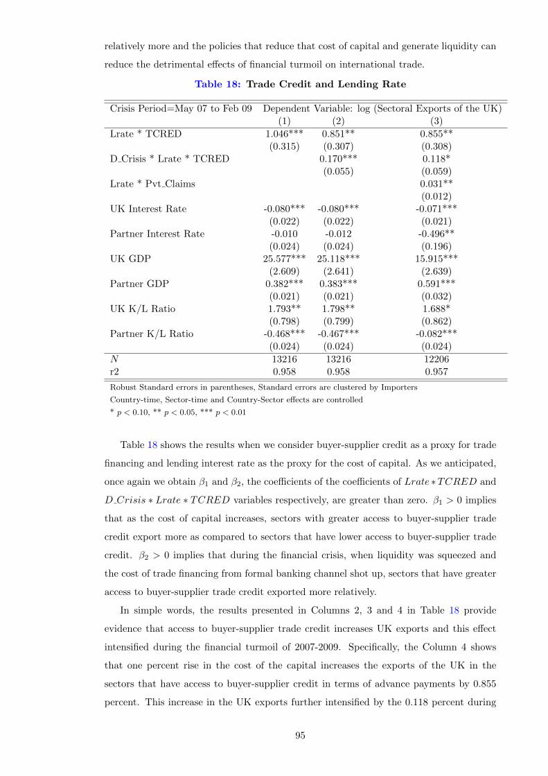
relatively more and the policies that reduce that cost of capital and generate liquidity can

reduce the detrimental effects of financial turmoil on international trade.

Table 18: Trade Credit and Lending Rate


Lrate * TCRED 1.046*** 0.851** 0.855**(0.315) (0.307) (0.308)

D Crisis * Lrate * TCRED 0.170*** 0.118*(0.055) (0.059)


UK Interest Rate -0.080*** -0.080*** -0.071***(0.022) (0.022) (0.021)


UK GDP 25.577*** 25.118*** 15.915***(2.609) (2.641) (2.639)

Partner GDP 0.382*** 0.383*** 0.591***(0.021) (0.021) (0.032)

UK K/L Ratio 1.793** 1.798** 1.688*(0.798) (0.799) (0.862)

Partner K/L Ratio -0.468*** -0.467*** -0.082***(0.024) (0.024) (0.024)

N 13216 13216 12206r2 0.958 0.958 0.957



* p < 0.10, ** p < 0.05, *** p < 0.01

Table 18 shows the results when we consider buyer-supplier credit as a proxy for trade

financing and lending interest rate as the proxy for the cost of capital. As we anticipated,

once again we obtain β1 and β2, the coefficients of the coefficients of Lrate ∗TCRED and

D Crisis ∗ Lrate ∗ TCRED variables respectively, are greater than zero. β1 > 0 implies

that as the cost of capital increases, sectors with greater access to buyer-supplier trade

credit export more as compared to sectors that have lower access to buyer-supplier trade

credit. β2 > 0 implies that during the financial crisis, when liquidity was squeezed and

the cost of trade financing from formal banking channel shot up, sectors that have greater

access to buyer-supplier trade credit exported more relatively.

In simple words, the results presented in Columns 2, 3 and 4 in Table 18 provide

evidence that access to buyer-supplier trade credit increases UK exports and this effect

intensified during the financial turmoil of 2007-2009. Specifically, the Column 4 shows

that one percent rise in the cost of the capital increases the exports of the UK in the

sectors that have access to buyer-supplier credit in terms of advance payments by 0.855

percent. This increase in the UK exports further intensified by the 0.118 percent during

95

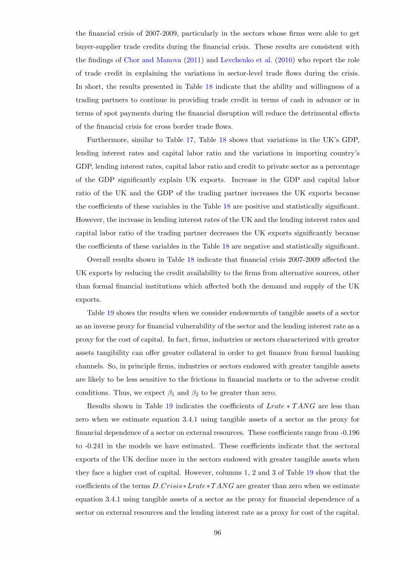
the financial crisis of 2007-2009, particularly in the sectors whose firms were able to get

buyer-supplier trade credits during the financial crisis. These results are consistent with

the findings of Chor and Manova (2011) and Levchenko et al. (2010) who report the role

of trade credit in explaining the variations in sector-level trade flows during the crisis.

In short, the results presented in Table 18 indicate that the ability and willingness of a

trading partners to continue in providing trade credit in terms of cash in advance or in

terms of spot payments during the financial disruption will reduce the detrimental effects

of the financial crisis for cross border trade flows.

Furthermore, similar to Table 17, Table 18 shows that variations in the UK’s GDP,

lending interest rates and capital labor ratio and the variations in importing country’s

GDP, lending interest rates, capital labor ratio and credit to private sector as a percentage

of the GDP significantly explain UK exports. Increase in the GDP and capital labor

ratio of the UK and the GDP of the trading partner increases the UK exports because

the coefficients of these variables in the Table 18 are positive and statistically significant.

However, the increase in lending interest rates of the UK and the lending interest rates and

capital labor ratio of the trading partner decreases the UK exports significantly because

the coefficients of these variables in the Table 18 are negative and statistically significant.

Overall results shown in Table 18 indicate that financial crisis 2007-2009 affected the

UK exports by reducing the credit availability to the firms from alternative sources, other

than formal financial institutions which affected both the demand and supply of the UK

exports.

Table 19 shows the results when we consider endowments of tangible assets of a sector

as an inverse proxy for financial vulnerability of the sector and the lending interest rate as a

proxy for the cost of capital. In fact, firms, industries or sectors characterized with greater

assets tangibility can offer greater collateral in order to get finance from formal banking

channels. So, in principle firms, industries or sectors endowed with greater tangible assets

are likely to be less sensitive to the frictions in financial markets or to the adverse credit

conditions. Thus, we expect β1 and β2 to be greater than zero.

Results shown in Table 19 indicates the coefficients of Lrate ∗ TANG are less than

zero when we estimate equation 3.4.1 using tangible assets of a sector as the proxy for

financial dependence of a sector on external resources. These coefficients range from -0.196

to -0.241 in the models we have estimated. These coefficients indicate that the sectoral

exports of the UK decline more in the sectors endowed with greater tangible assets when

they face a higher cost of capital. However, columns 1, 2 and 3 of Table 19 show that the

coefficients of the terms D Crisis∗Lrate∗TANG are greater than zero when we estimate

equation 3.4.1 using tangible assets of a sector as the proxy for financial dependence of a

sector on external resources and the lending interest rate as a proxy for cost of the capital.

96

Table 19: Tangible Assets and Lending Rate


Lrate * TANG -0.196** -0.241*** -0.208**(0.070) (0.067) (0.077)

D Crisis * Lrate * TANG 0.041** 0.029*(0.016) (0.015)


UK Interest Rate 0.057** 0.056** 0.056*(0.026) (0.026) (0.030)


UK GDP 24.088*** 23.103*** 14.298***(2.121) (2.211) (2.368)

Partner GDP 0.382*** 0.383*** 0.589***(0.021) (0.021) (0.031)

UK K/L Ratio 1.818** 1.822** 1.711*(0.797) (0.797) (0.861)

Partner K/L Ratio -0.468*** -0.467*** -0.082***(0.024) (0.024) (0.024)

N 13216 13216 12206r2 0.958 0.958 0.957



* p < 0.10, ** p < 0.05, *** p < 0.01

97

These coefficients indicate that during the financial crisis 2007-2009 in which reserves of the

financial institutions were decreased dramatically, banks were reluctant to give loans to the

firms and interest rates were gone up, the UK sector level exports increased in the sectors

that were endowed with greater tangible assets because they can present more assets as a

collateral to the banks to get loan. This also implies that in the presence of high cost of

capital, UK export performance is better in the sectors characterized by greater tangible

assets. Moreover, the coefficient of the triple interaction term (D Crisis∗Lrate∗TANG),

β2 is greater than zero which implies that the positive impact of tangible assets on UK

export performance became markedly stronger during the 2007-2009 financial crisis.

With regards to other control variables used in the models, Table 19 shows that GDP

and the capital labor ratio of the UK significantly determine UK sectoral exports. Columns

2, 3 and 4 of the Table 19 show that the sectoral exports of the UK increases significantly

with the increase in GDP and the capital labor ratio of the UK. One percent increase in

GDP of the UK increases the exports of the UK by 14.298 percent and one unit increase in

capital labor ratio of the UK increases the exports of the UK by 1.711 units. This implies

that GDP and the capital labor ratio of the UK significantly contribute to the exports of

the UK.

Column 4 of Table 19 shows that the financial variables of importing country, claims

on private sectors as a percentage of GDP and partner country interest rates significantly

affect UK exports. A one percent rise in the partner country’s claims on private sector as

a percentage of the GDP increases UK exports by 0.031 percent whereas a one percent

rise in the importing country’s interest rates decreases UK exports by 0.507 percent. This

implies that the rise in the financial resources of the consumers living in trading partners

increases demand for goods imported from the UK whereas the rise in the cost of financial

resources in the importing country reduces the demand for goods imported from the UK.

Moreover, partner country GDP and the capital-labor ratio significantly determine the UK

exports. Importing country GDP and UK exports are positively related whereas importing

country capital labor ratio and UK exports move in the opposite direction. This implies

that increases in the GDP of trading partners boost their imports from the UK whereas an

increase in capital relative to the labor of the trading partners discourages imports from

the UK. This result is quite meaningful because a rise in GDP of the importing countries

increases their income level which in turn boosts demand for imported goods, while an

increase in the capital labor ratio of trading partners indicate that their capacity to produce

and meet the their demand for a product domestically is enhanced. Consequently, their

demand for imported goods decreases.

Overall, results shown in Table 19 indicate that the 2007-2009 financial crisis had

severe consequences for UK exports particularly for the exports of the sectors with lesser

98

endowments of the tangible assets. Furthermore, the 2007-2009 financial crisis exerted its

pressure on UK exports by affecting both the demand and supply sides of exports. Results

in Table 19 also suggest that financial crisis hits the exports of financially constrained

firms relatively more and policies that reduce that cost of capital and generate liquidity

can reduce the detrimental effects of financial turmoil on international trade.

Once again our results are consistent with the findings of Chor and Manova (2011) who

report that countries with higher interbank rates export more in the sectors intensive in

tangible assets. They also provide evidence of stronger comparative advantage of a sector

with greater tangible assets has in exporting its products during the financial crisis over

the sector with lower tangible assets. Similarly, Iacovone and Zavacka (2009) also report

that the decline in exports of the sector endowed with fewer tangible assets during the

financial crisis.

Table 20: Leverage and Lending Rate


Lrate * Leverage -0.240 -0.285* -0.254(0.157) (0.160) (0.165)

D Crisis * Lrate * Leverage 0.040** 0.036**(0.017) (0.017)


UK Interest Rate 0.085 0.085 0.070(0.055) (0.055) (0.061)


UK GDP 26.753*** 26.235*** 16.435***(2.695) (2.733) (3.032)

Partner GDP 0.382*** 0.383*** 0.595***(0.021) (0.021) (0.035)

UK K/L Ratio 1.812** 1.818** 1.702*(0.799) (0.799) (0.865)

Partner K/L Ratio -0.468*** -0.467*** -0.079***(0.024) (0.024) (0.025)

N 13216 13216 12206r2 0.958 0.958 0.957



* p < 0.10, ** p < 0.05, *** p < 0.01

Actually, a higher proportion of the tangible assets in firms’ total assets provides

higher protection to banks because banks can recover their loans by selling these assets

if a firm defaults. So, banks prefer to lend to firms with greater tangible assets. This

relationship between tangible assets and access to financial resources makes sectors with

intensive tangible assets less vulnerable to financial markets disruptions. Therefore, export

99

performance of the sectors with greater tangible assets remains relatively stable during

financial crisis.

Table 20 shows results when we consider leverage as a proxy for financial dependence

of a sector on external resources. Basically, leverage indicates the riskiness of a firm.

A firm with larger values of leverage is more risky than a firm with a lower value of the

leverage. So, it is likely that firms characterized by higher leverage face problems in getting

funds from financial institutions. Particularly, during a liquidity crisis banks hesitate to

lend to highly leveraged firms. Therefore, such firms are likely to face disruption in their

exporting activity during the financial crisis. Hence, we expect coefficients of both single

and double interaction terms, i.e., the parameters of IBrateuk,t × LEV ERAGEuk,k and

DCrisis × IBrateuk,t × LEV ERAGEuk,k to be less than zero. In general, the leveraged

firms are big in their sizes and have more collateralizable assets which they can present as

a collateral to get funds from the financial resources from the financial institutions. If this

is the case, then leverage firms may get the funds easily from the banks even under the

crisis situations. Under this scenario the coefficients of both single and double interaction

terms, i.e., the parameters of IBrateuk,t × LEV ERAGEuk,k and DCrisis × IBrateuk,t ×

LEV ERAGEuk,k can be greater than zero. However, if the crisis becomes so severe that

banks are unable to give loans to leveraged firms, then coefficient of double interaction

terms, i.e., the parameters of DCrisis × IBrateuk,t × LEV ERAGEuk,k will be less than

zero.

Table 20 shows results when we consider leverage as a proxy for financial dependence

of a sector on external resources. Columns 2, 3 and 4 of the Table 20 show that the

coefficients of single interaction terms i.e., the parameters of IBrateuk,t×LEV ERAGEuk,kare negative and ranges from -0.240 to -0.285 depending on the control variable used

in the model. This implies that in the presence of higher cost of trade financing the

UK exports less in sectors characterized by higher values of leverage. This result seems

reasonable because the leverage indicates the riskiness of a firm. A firm with larger values

of leverage is more risky than a firm with a lower value of the leverage. So, it is likely

that firms characterized by higher leverage face problems in getting funds from financial

institutions. However, this effect is statistically significant only in case the model 2.

Moreover, Column 3 and 4 of the Table 20 indicate that the coefficients of the DCrisis ×

IBrateuk,t × LEV ERAGEuk,k is positive and ranges from 0.036 to 0.040 which implies

that the exports of the leveraged sector have increased during the financial crisis 2007-

2009. Specifically, Column 4 of the Table 20 indicates that one unit rise in leverage of a

firm increases the UK exports by 0.036. This effect of the leverage on the UK exports is

statistically significant. The leveraged firms have exported more during the financial crisis

2007-2009 because in general, the highly leveraged firms are big in their sizes and have

100

more collateralizable assets which they can present as a collateral to get funds from the

financial institutions.

Furthermore, similar to Tables 17, 18 and 19, the Table 20 shows that variations in the

UK’s GDP and capital labor ratio and the variations in importing country’s GDP, lending

interest rates, capital labor ratio and credit to private sector as a percentage of the GDP

significantly explain the variations in the UK exports. Increase in the GDP and capital

labor ratio of the UK and the GDP of the trading partner increases the UK exports

because the coefficients of these variables in the Table 20 are positive and statistically

significant. However, increase in the lending interest rates and capital labor ratio of the

trading partner decrease the UK exports significantly because the coefficients of these

variables in the Table 20 are negative and statistically significant.

Overall, Tables 17, 18, 19 and 20 indicate that the financial crisis 2007-2009 had

affected the UK exports significantly. In particular, a decline in UK sector level exports

during the financial crisis has resulted in severe consequences for the real economy. On

one hand the tight conditions for access to financial resources during the crisis severely

affected firms’ ability to invest in new and in existing projects leading to fall in output and

employment. On the other hand, a gloomy picture of the economy along with the rise in

unemployment decreased consumers’ income which shattered consumers’ confidence and

their demand for products fell sharply across the globe. As a result, exports fell down.

3.5.2 Sectoral Analysis

So for we have discussed our finding regarding the overall effects of the 2007-2009 global

financial crisis on UK exports. We presented the evidence that financially vulnerable

sectors export less when they face higher costs of capital and this effect had intensified

during the 2007-2009 financial crisis when financial conditions not only in the UK but in

the whole world became tight. Moreover, these negative effects were more prominent in

the sectors endowed with less tangible assets, having lower access to buyer-supplier credit

and having higher values of leverage.

In this section we report our findings regarding the response of exports of different

sectors to the 2007-2009 financial turmoil. We define a firm as a financially constrained

firms if it require funds from external sources to carry out its production activities and

have a lower access to funds from the external sources. We have used four proxies to

represent financial constraints of a firm. They include the External finance, defined as a

ratio of capital expenditure not financed by the internal cash flows from operation to the

investment (EXTFIN), Trade credit, defined as a ratio of trade credit to the book value

of total assets of firm (TCRED), Tangible assets, defined as ratio of total tangible assets

to the book value of total assets of firm (TANG) and Leverage, defined as ratio of total

101

debt to the book value of total assets of a firm. We have calculated these proxies for each

firm included in the sector and then have taken a median value of all the firms in a sector

to represent a financial constraints of a sector. In simple words a sector is a financially

constrained if on average firms included in a sector have lower access to external finance

or have lower access to trade credit or have lesser collateralizable assets to get loans from

banks or other financial institutions. Table B.5 in Appendix B shows the average values

of the proxies used to represent the financial constraints of different sector.

102

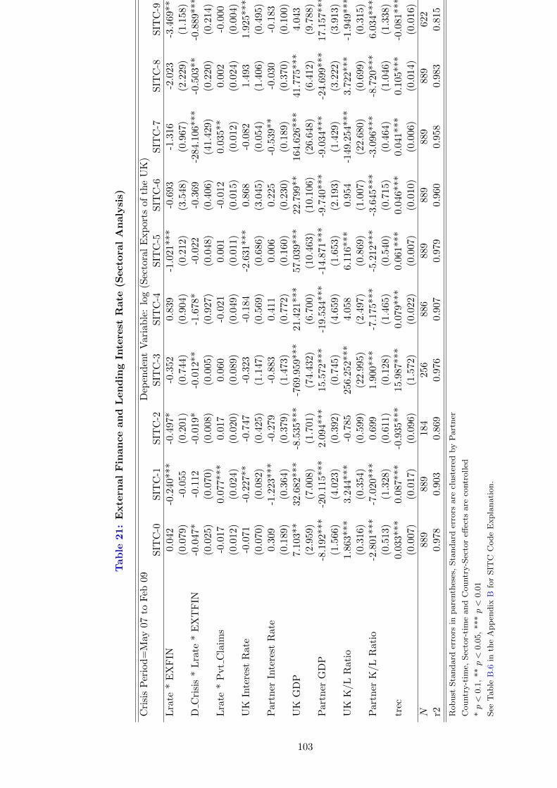
Tab

le21:

Exte

rnal

Fin

an

ce

an

dL

en

din

gIn

tere

stR

ate

(Secto

ral

An

aly

sis)

Cri

sis

Per

iod

=M

ay07

toF

eb09

Dep

end

ent

Var

iab

le:

log

(Sec

tora

lE

xp

ort

sof

the

UK

)S

ITC

-0S

ITC

-1S

ITC

-2S

ITC

-3S

ITC

-4S

ITC

-5S

ITC

-6S

ITC

-7S

ITC

-8S

ITC

-9

Lra

te*

EX

FIN

0.04

2-0

.240

***

-0.4

97*

-0.3

520.

839

-1.0

21***

-0.6

93

-1.3

16

-2.0

23

-3.4

69**

(0.0

79)

-0.0

55(0

.201

)(0

.744

)(0

.904

)(0

.212)

(3.5

48)

(0.9

67)

(2.2

29)

(1.1

58)

DC

risi

s*

Lra

te*

EX

TF

IN-0

.047

*-0

.112

-0.0

19*

-0.0

12**

-1.6

78*

-0.0

22

-0.3

69

-284.1

06***

-0.5

03**

-0.8

89***

(0.0

25)

(0.0

70)

(0.0

08)

(0.0

05)

(0.9

27)

(0.0

48)

(0.4

06)

(41.4

29)

(0.2

20)

(0.2

14)

Lra

te*

Pvt

Cla

ims

-0.0

170.

077*

**0.

017

0.06

0-0

.021

0.0

01

-0.0

12

0.0

35**

0.0

02

-0.0

00

(0.0

12)

(0.0

24)

(0.0

20)

(0.0

89)

(0.0

49)

(0.0

11)

(0.0

15)

(0.0

12)

(0.0

24)

(0.0

04)

UK

Inte

rest

Rat

e-0

.071

-0.2

27**

-0.7

47-0

.323

-0.1

84-2

.631***

0.8

68

-0.0

82

1.4

93

1.9

25***

(0.0

70)

(0.0

82)

(0.4

25)

(1.1

47)

(0.5

69)

(0.6

86)

(3.0

45)

(0.0

54)

(1.4

06)

(0.4

95)

Par

tner

Inte

rest

Rat

e0.

309

-1.2

23**

*-0

.279

-0.8

830.

411

0.0

06

0.2

25

-0.5

39**

-0.0

30

-0.1

83

(0.1

89)

(0.3

64)

(0.3

79)

(1.4

73)

(0.7

72)

(0.1

60)

(0.2

30)

(0.1

89)

(0.3

70)

(0.1

00)

UK

GD

P7.

103*

*32

.682

***

-8.5

35**

*-7

69.9

59**

*21

.421

***

57.0

39***

22.7

99**

164.6

26***

41.7

75***

4.0

43

(2.9

59)

(7.0

08)

(1.7

01)

(74.

432)

(6.7

00)

(10.4

63)

(10.1

06)

(26.6

48)

(6.4

12)

(9.7

88)

Par

tner

GD

P-8

.192

***

-20.

115*

**2.

094*

**15

.572

***

-19.

534*

**-1

4.8

71***

-9.7

40***

-9.0

34***

-24.6

99***

17.1

57***

(1.5

66)

(4.0

23)

(0.3

92)

(0.7

45)

(4.6

59)

(1.6

53)

(2.1

93)

(1.4

29)

(3.2

22)

(3.9

13)

UK

K/L

Rat

io1.

863*

**3.

244*

**-0

.785

256.

252*

**4.

058

6.1

16***

0.9

54

-149.2

54***

3.7

22***

-1.9

49***

(0.3

16)

(0.3

54)

(0.5

99)

(22.

995)

(2.4

97)

(0.8

69)

(1.0

07)

(22.6

80)

(0.6

99)

(0.3

15)

Par

tner

K/L

Rat

io-2

.801

***

-7.0

20**

*0.

699

1.90

0***

-7.1

75**

*-5

.212***

-3.6

45***

-3.0

96***

-8.7

20***

6.0

34***

(0.5

13)

(1.3

28)

(0.6

11)

(0.1

28)

(1.4

65)

(0.5

40)

(0.7

15)

(0.4

64)

(1.0

46)

(1.3

38)

trec

0.03

3***

0.08

7***

-0.9

35**

*15

.987

***

0.07

9***

0.0

61***

0.0

46***

0.0

41***

0.1

05***

-0.0

81***

(0.0

07)

(0.0

17)

(0.0

96)

(1.5

72)

(0.0

22)

(0.0

07)

(0.0

10)

(0.0

06)

(0.0

14)

(0.0

16)

N88

988

918

425

688

6889

889

889

889

622

r20.

978

0.90

30.

869

0.97

60.

907

0.9

79

0.9

60

0.9

58

0.9

83

0.8

15

Robust

Sta

ndard

erro

rsin

pare

nth

eses

,Sta

ndard

erro

rsare

clust

ered

by

Part

ner

Countr

y-t

ime,

Sec

tor-

tim

eand

Countr

y-S

ecto

reff

ects

are

contr

olled

*p<

0.1

,**p<

0.0

5,

***p<

0.0

1

See

Table

B.6

inth

eA

pp

endix

Bfo

rSIT

CC

ode

Expla

nati

on.

103

We classify UK exports at the sectoral level using Standard International Trade Clas-

sification (SITC) Revision 3. Details of these codes are given in Table B.6 in Appendix

B.

Table 21 presents results when we estimate equation 3.4.1 for each sector separately

using external finance as proxy for financial dependence of the sector and lending interest

rate as a proxy for the cost of capital. The coefficients of the Lrate ∗ EXTFIN ranges

from -0.3.469 to 0.839. These coefficients implies that the marginal sensitivity of the

UK sectoral exports to the financial vulnerability caused by the changes in the cost of

the capital varies from sector to sector depending on their sizes, their requirements of

funds from the external sources and availability of the required funds from formal and

non-formal financial institutions. Overall, results given in Table 21 highlight that eight

out of ten sectors tend to reduce their exports when they face higher cost of capital.

However, only five sectors become financially vulnerable when the cost of capital increases

and significantly reduce their exports. These sectors are Beverages and Tobacco (SITC-

1), Crude materials, inedible except fuels (SITC-2), Chemical and related products n.e.s

(SITC-5) and Commodities and transactions not classified elsewhere in the SITC (SITC-

9).

Note that in Table 21, β2 i.e the coefficient of D Crisis∗Lrate∗EXTFIN is less than

zero and statistically significant for all sectors except Beverages and Tobacco (SITC-1)

and Manufactured goods classified chiefly by material (SITC-6) sectors. The coefficient of

D Crisis∗Lrate∗EXTFIN ranges from -284.106 to -0.012 which indicates that financial

crisis 2007-2009 affected the exports of different sector differently. Table 21 shows that

the financial crisis 2007-2009 had the most severe consequences for the exports of the

Machinery and transport equipment (SITC-7) sector and had the least impact on the

exports of beverages and tobacco (SITC-1) sector. Overall the coefficients of the term

D Crisis ∗ Lrate ∗ EXTFIN indicate that the reduction in sector level exports of the

UK intensified during the 2007-2009 global financial crisis. Overall, Table 20 and results

reported in Table 21 point out that the UK sector level exports depend more on external

finance. Therefore, they were severely affected by the 2007-2009 global financial crisis.

Other variables which significantly affected the UK sectoral exports are the GDP and

the capital-labor ratio of the UK and the GDP and the capital labor ratio of the trading

partners of the UK. These variables significantly explain the variations in the exports of

all the sectors. Lending interest rates of the UK and the lending interest rates and claims

on private sectors of the importing countries are insignificant in explaining the variations

in the exports of most of the sectors when we consider their impact on the exports of a

single sector at a time.

On the whole, Table 21 provides the evidence that the net effect of the 2007-2009

104

financial crisis on UK sectoral exports is negative and consistent with the existing lit-

erature. For instance, Jansen and von Uexkuell (2010) state that the net effect of the

global financial crisis on trade is negative. In fact the loss in economic activity due to

financial turmoil 2007-2009 resulted in a decline in incomes of consumers living in the

UK as well as the consumers living in the other parts of the globe. In turn, demand for

imports declined across the globe leading to a contraction in the volume of international

trade overall . Our finding that exports of ”Food and Live Animals” decreased during

the financial crunch support this fact. Actually, the decrease in economic activity and the

rise in unemployment during the financial crisis resulted in a decrease of incomes of the

people. As a result, demand for food and live animal decreased because a big chunk of the

income, people spend on their food. Jansen and von Uexkuell (2010) report a fall income

of along with a rise in prices of food items during the crisis as major reasons of fall in

export of food items.

Moreover, the results given in Table 21 suggest that the financial crisis created the

rippling effects for sector level export of the UK. Declines in foreign sales of one sector

have generated a decline in exports of the other sectors. For example, negative coefficients

of the triple interaction terms D Crisis ∗ Lrate ∗EXTFIN point out that exports of all

sectors declined during the financial crisis. This overall decline in exports led to decrease

in the demand for transport and allied sectors which contribute to boost the trade. The

results shown in columns 5, 8, 9 and 10 of the Table 21 may support this argument and

point out that the decline in the exports of Animal and vegetable oils, fats and waxes

(SITC-4), Miscellaneous manufactured articles (SITC-8), Commodities and transaction

not classified elsewhere in the SITC (SITC-9) and Machinery and Transport Equipment

(SITC-7) exports significantly declined during crisis period. As a result demand for lor-

ries and trucks used to transport tradable commodities from one destination to another

destination declined which contributed to the decline in demand for Minerals, Fuels, Lu-

bricants and related material (SITC-3) leading to the decrease in the exports of Fuels,

Lubricants and related material (SITC-3). Results provided in column 4 of Table 21 favor

this observation.

We find that except for Food and live animal (SITC-0) and Animal and vegetable

oils, fats and waxes (SITC-4), all other sectors that require external financing reduce their

foreign sales when they experience a rise in the interest rate. However, columns 3, 4, 7 and

11 in Table 21 show that an increase in interest rates leads to a significant reduction in

exports of Beverages and tobacco (SITC-1), Crude materials, inedible except Fuel (SITC-

2), Chemical and Related Products, n.e.s (SITC-5), Commodities and transactions not

classified elsewhere in the SITC (SITC-9).

105

3.5.3 Sensitivity Analysis

We check the robustness of our results in two ways. First, instead of the lending interest

rate, we use the overnight interbank rate as the proxy for cost of capital. However, the

proxies to represent financial vulnerability of the sector; EXTFIN, TCRED and LEVER-

AGE remain the same. Second, we apply the instrumental variable (IV) technique to

estimate our model because current period exports may be driven by previous period

exports and may become endogenous. If this is the case then OLS gives biased and incon-

sistent estimates whereas the IV approach takes care of endogeneity problems and gives

unbiased and consistent estimates.

3.5.4 An alternative Proxy for Cost of Capital

Table 22 reports the results when we use external finance as a proxy for financial depen-

dence of a sector and the overnight interbank rate as a proxy for the cost of capital. Once

again, columns 2, 3 and 4 of the Table 22 show that in the presence of a higher overnight

interbank rate, the UK exports less in the sectors which depend more on external resources.

Likewise, we find that the tendency of decline in the UK sector level exports in response to

a rise in the overnight interbank rate became stronger and statistically significant during

the 2007-2009 financial crisis when overnight interbank rates shot up. Hence, our findings

that sector level exports of the UK are finance dependent and become vulnerable when

financial markets face liquidity crisis does not change with the change in the proxy for cost

of capital. Indeed, Table 22 shows that financial variables of the UK significantly affect

UK exports. Moreover, importing country financial variables like interest rates and claims

on the private sector play a significant role in explaining the variations in UK sector level

exports. Furthermore, partner country GDP and capital-labor ratio significantly affect

UK exports. This implies that demand side of the UK exports is as equally important as

the supply side of the UK exports. This indicates that disruptions in financial markets

exert their pressure on exports through interest rates, here the overnight interbank rate,

and affect both demand and supply of exports significantly.

Overall, the results reported in Table 22 and in Tables B.1, B.2 and B.3 in Appendix

B are similar to the results presented in the Tables 17, 18, 19 and 20. Only a slight

variation in values of the parameters exists, but the sign and significance of parameters

do not change when we use the overnight interbank rate as a proxy for the cost of capital

instead of lending rate to measure cost of capital. On the whole, Table 22 and Tables

B.1, B.2 and B.3 in Appendix B show that when the overnight interbank rate increases

UK sector level exports contract. Furthermore, this contraction in exports in response

to a rise in the overnight interbank rate occurs relatively more in sectors which depend

106

Table 22: External Finance and Overnight Interbank Rate


IBrate * EXTFIN -0.013* -0.007 -0.007(0.007) (0.007) (0.007)

D Crisis * IBrate * EXTFIN -0.015*** -0.014**(0.005) (0.005)

IBrate * Pvt Claims 0.010***(0.002)

UK Interest Rate 0.003 -0.0003 -0.005(0.011) (0.010) (0.013)

Partner Interest Rate -0.024* -0.024* -0.143***(0.012) (0.012) (0.026)

UK GDP 5.541* 5.114 5.652(3.055) (3.039) (3.551)

Partner GDP 1.002*** 1.001*** 1.070***(0.065) (0.064) (0.026)

UK K/L Ratio -1.872** -1.887** -2.350***(0.676) (0.674) (0.689)

Partner K/L Ratio 0.546*** 0.545*** 0.617***(0.089) (0.089) (0.035)

N 13916 13916 12566r2 0.939 0.939 0.935



* p < 0.10, ** p < 0.05, *** p < 0.01

107

more on external finance, have lower access to buyer-supplier trade credit and have lower

values of the leverage. In addition, this response of UK exports to changes in the overnight

interbank rate intensified further during the 2007-2009 financial crisis.

In sum, the results reported in Table 22 and in Tables B.1, B.2 and B.3 in Appendix

B indicate that our results are robust and do not change with the change in proxy used to

measure the cost of capital. UK exports behave in a similar way in response to variations

in overnight interbank rates and in response to fluctuations in the lending rates which we

have used to measure the cost of capital.

3.5.5 Instrumental Variable (IV) Technique

Current period exports may depend on exports in the previous period. If this is the case

then OLS estimates become inconsistent due to possible endogeneity between errors and

the lagged dependent variable. Therefore, to resolve this problem and to get consistent

estimates we estimate equation 3.4.2 using an instrumental variable approach.

Table 23 presents the results when we estimate equation 3.4.2 using the instrumental

variable approach. Columns 2, 3 and 4 of Table 23 report the results when use LEVER-

AGE, EXTFIN and TCRED as proxies for financial dependency of the sector. Table 23

shows that previous period exports significantly determine current period exports. More-

over, coefficients of lag period exports in Table 23 indicate that previous period exports

positively affect current exports. This finding suggests that the sectors which exported

more in the previous period are likely to export more in the current period.

The results presented in Table 23 also suggest that the UK exports more in the sectors

which are less dependent on external finance when they experience higher cost of capital.

This intensity of decrease in exports due to rise in the cost of capital become more in-

tensified during the financial crisis. For example Column 2 of the Table 23 shows that a

one percent rise in the cost of the capital increases the exports of firms which have higher

leverage value by 0.025 percent. This makes sense because normally the high leveraged

firms are normally bigger in their sizes and can afford and manage to get funds from the

banks even when the cost of the capital has increased. However, during the financial crisis

of 2007-2009 the leveraged firms were unable to get the loans from banks because the

banks were unable to give loans to bigger firms due to the lack of funds. The coefficient

of the D Crisis * IBrate * Fin Vul in Column 1 of the Table 23 shows this phenomenon.

This implies that even the high leveraged firms’ exports declined during the financial

crisis because they were unable to get funds to finance their production to fulfill their

export orders during the financial crisis. The marginal decrease in the exports of the

leveraged firms due to unavailability of the funds during the financial crisis of 2007-2009

is 0.024. In addition, Table 23 shows that a rise in the overnight interbank rate leads to

108

Table 23: IV Results new External Finance and Overnight Interbank Rate

Crisis Period=May 07 to Feb 09 Dependent Variable: log (Sectoral Exports of the UK)Fin vulnerability measure: (LEVERAGE) (TCRED) (EXTFIN)

l.Exports 0.902*** 0.901*** 0.910***0.011 0.011 -0.008

IBrate * Fin Vul 0.025* 0.072*** -0.001**(0.013) (0.017) (0.001)

D Crisis * IBrate * Fin Vul -0.024*** -0.077*** -0.0001(0.007) (0.028) (0.001)

IBrate * Pvt Claims 0.002* 0.002** -0.002***(0.001) (0.001) (0.0003)

UK Interest Rate -0.005 -0.005* -0.003*(0.005) (0.003) (0.001)

Partner Interest Rate -0.038** -0.039** 0.019***(0.016) (0.016) (0.003)

UK GDP 1.498*** 1.503*** 0.910***(0.193) (0.199) (0.146)

Partner GDP 0.004 0.004 0.036(0.043) (0.043) (0.037)

UK K/L Ratio -0.342*** -0.338*** -0.232***(0.065) (0.066) (0.044)

Partner K/L Ratio 0.004 0.005 0.045**(0.037) (0.038) (0.018)

N 11734 11734 12204r2 0.351 0.352 0.353Hansen Test 0.983 0.990 0.912

Robust Standard errors in parentheses, Standard errors are clustered by Partner

Time, Reporter, Partner and Sector fixed effects are controlled

* p < 0.1, ** p < 0.05, *** p < 0.01

a decline in UK exports, especially in the sectors which depend more on external finance,

have lower access to buyer-supplier trade credit and have higher leverage values.

Moreover, Column 3 of the Table 23 indicates that UK firms with higher access to

buyer-supplier trade credit export more relatively than the firms who are unable to get

buyer-supplier trade credit to finance their production activities to fulfill their export

orders. The coefficient of IBrate * Fin Vul Column 3 of the Table 23 shows that a one

percent rise in the cost of the capital increases exports of firms which have a higher access

to the buyer-supplier trade credit by 0.072 percent. However, the coefficient of the D Crisis

* IBrate * Fin Vul in Column 3 of the Table 23 indicates that during the financial crisis

UK exports decreased by 0.077 percent. This implies that the financial crisis of 2007-

2009 was so intensive that it had depleted the buyer-supplier credit and as a result UK

exports decreased because firms were unable to get finances from the sources other than

the formal financial institutions to finance their production activities to fulfill their export

orders. This implies that financial crisis 2007-2009 has significantly decreased the exports

of the firms who have lesser access to buyer-supplier trade credit.

109

Column 4 of the Table 23 shows the results when we use external finance as a proxy

for financial vulnerability of a firm. The coefficient of the IBrate * Fin Vul in Column 4

of the Table 23 indicates that as the cost of capital increases the UK exports significantly

decreases because it raises overall cost of the production and their prices which makes

the UK goods less competitive in the international markets. As a results their demand

decreases leading to decrease in the UK exports. Moreover, the exports decreases because

some firms particularly the smaller firms cannot afford to get loan from the banks at a

higher cost. So their productions and exports both fall. In addition, coefficient of the

IBrate * Fin Vul in Column 4 of the Table 23 indicates that one percent rise in the cost of

capital leads to 0.001 percent decrease in the UK exports. This intensity of the decrease

in UK exports due to rise in the cost of capital intensified further during the financial

crisis 2007-2009 when cost of capital i.e. the interest rate shot up. The coefficient of the

D Crisis * IBrate * Fin Vul in Column 4 of the Table 23 indicates that UK exports have

decreased by 0.0001 percent due to one percent in the cost of the capital but this effect is

statistically insignificant.

From supply side the other variables which effects the UK exports significantly include

GDP of the UK, lending interest rates and the capital labor ratio of the UK. Results given

in the Table 23 shows that GDP significantly increases the UK exports. Whereas the

lending interest rates and the capital labor ratio of the UK significantly decrease the UK

exports. However, lending interest rate is significant only in two models. Furthermore,

one percent rise in the GDP of the UK increases the UK exports more than one percent.

This implies that the UK exports increase with the increase in GDP of the UK . However,

the negative coefficients of the capital labor ratio and the interest rates of the UK indicate

that supply of the UK exports contracts with the increase in capital labor ratio and with

the increase in interest rate.

On the demand side of the UK exports the Table 23 shows that partner country lending

interest rates significantly reduces the UK exports. Whereas partner country claims on

the private sector significantly increases the UK exports. This implies that the increase in

financial resources of the consumers living in the trading partners of the UK significantly

increases UK exports. However, the rise in lending interest rates or the cost of the financial

resources of the consumers living in the trading partner countries significantly reduces UK

exports.

Overall results shown in the Table 23 indicate that UK exports are significantly influ-

enced by the financial variables of the UK as well as the financial variables of the trading

partners. In simple words, both the supply and demand sides matters for UK exports.

Furthermore, we find that the negative impact of a rise in the cost of capital on exports

of the sector which depends more on external finance, having limited access to trade credit

110

and higher values of leverage became stronger during the financial crisis 2007-2009. This

implies that the 2007-2009 financial crisis has severely hit UK sector level exports.

Overall, Table 23 shows that exporting country’s financial variables significantly ex-

plain the variations in exports. Similarly, the financial variables of importing country

significantly explain the fluctuations in the UK sector level exports as well. Once more,

we find that GDP and the capital labor ratio of the UK and partner country’s claims on

private sector significantly determine UK exports. In a nutshell our major findings do not

change with the change in methodology adopted to estimate the model.

The results explained in Sections 3.5.3, 3.5.4 and 3.5.5 show that overall our findings

are robust and remain consistent even if we change the proxy to measure cost of capital

or if we change the technique to estimate the parameters of the model.

3.6 Conclusions

In this chapter we analyzed the impact of the 2007-2009 global financial crisis on UK

trade with its major trading partners. Our sample covers monthly exports of ten sectors

going to twenty five major importers of the UK from January 2002 to September 2011.

We applied Ordinary Least Square (OLS) and Instrumental Variable (IV) techniques to

estimate our empirical models. Exploiting variations in the cost of capital over time as

well as fluctuations in financial vulnerability across different sectors, we show that credit

conditions are an important channel through which financial turmoil affects the volume of

UK exports. Specifically, we show that with higher lending rates and thus tighter credit

market conditions UK exported less during the 2007-2009 financial crisis. Moreover, these

negative effects become stronger for sectors with limited access to buyer-supplier trade

credit, with fewer collateralizable assets and with higher dependency on external financing.

We also find that adverse credit conditions affect both the supply and demand sides of

exports and play a significant role in determining the supply and demand for UK exports.

We find that along with the financial conditions in the trading partners, the volume of GDP

and capital labor ratios of the importing countries are the main factors in determining the

demand for the UK exports, whereas the supply of the UK exports is driven by financial

conditions, GDP and the capital-labor ratio of the UK.

In general, our findings imply that adverse credit conditions are an important channel

through which financial turmoil transmits its effect to international trade flows of the UK.

These effects of the credit crunch on UK exports hold even after controlling for GDP, the

factors of production and the cost of capital in trading partners of the UK as well as the

GDP and the capital-labor ratio of the UK. Moreover, our findings regarding the impact

of financial conditions on the UK exports are robust and do not change with changes in

the proxy used to represent the cost of capital or with change in the measure used to

111

represent financial dependency of the sector on external resources.

Overall, our findings suggest that policy interventions that reduce the cost of capital

will be really helpful in reducing substantially the detrimental effects of severe financial

disruptions on international trade flows.

112

Chapter 4

Trade Creation and Diversion Effects of the EuropeanUnion

4.1 Introduction

Regionalism has re-emerged as one of the key developments in international trade relations.

511 Regional Trade Agreements (RTAs) have been notified to World Trade Organization

(WTO) as of January, 2012, out of which 319 RTAs are in force. Among the RTAs 90

percent are Free Trade Areas (FTA) and 10 percent are Customs Unions (CU)10. A Free

Trade Area is an agreement in which two or more than two countries agree

to remove all the tariff and non-tariff barriers and the quantitative restric-

tions on their mutual trade. However, each member of the group is free to

adopt and maintain any tariff or regulations on the trade with non-member

country. However, a Custom Union is an agreement in which two or more

than two countries agree to remove all the tariff and non-tariff barriers and

the quantitative restrictions on their mutual trade, plus a common external

tariff on the trade with non-member countries11. Most global trade takes place

among the countries associated with these agreements. According to Clarete et al. (2003)

97 percent of international trade in 2000 was among the countries that had joined at least

one of the RTAs. However, this share was 72 percent in 1990. Similarly, 21 Asia-Pacific

Economic Cooperation (APEC) economies, collectively, account for 44 percent of world

trade12. Likewise, in the context of European Union (EU), the EUCOM (2009) report

states that EU is the chief economic area in the world with 30 percent of global GDP and

17 percent of the global trade.

Unification of the trade policies changes the consumption and production behavior of

member and non-member countries. In addition, economic integration affects the welfare

of the people living in member and non-member countries. These changes in consumption,

production and in welfare can be measured in terms of trade creation and trade diversion

generated by the RTAs. Trade creation (TC) takes place when production shifts to a low

cost member country, and consumption shifts from domestic goods to imported goods.

Trade diversion (TD) is a phenomenon in which production shifts to a low cost member

country, which may not be the lowest in the world. Moreover, consumption shifts from

imported goods of a non-member country to goods imported from a member country.

10For detail, see http://www.wto.org/english/tratop e/region e/region e.htm 07-7-2012.11see Figure 21 in Appendix C for levels of economic integration12For detail, see http://www.ustr.gov/countries-regions/japan-korea-apec/apec 08-03-2010.

113

The mushroom growth of RTAs in the world and an unprecedented increase in the share

of global trade taking place among the members of these RTAs catches the attention of

researchers and economists to test the effects of RTAs on trade flows. A number of studies

have explored the theoretical and empirical relations between economic integration and

trade flows to seek the answers to questions such as how an RTA affects the trade flows of

members and non-member countries? What are the channels through which an RTA affects

the trade? For example, Viner (1950), Lipsey (1957),Bhagwati (1971), Gehrels (1956),

Riezman (1979) and Kowalczyk (2000) have discussed the theoretical framework about

trade creation, trade diversion and the welfare effects of an RTA. They have developed

the conditions through which we can decide whether an RTA diverts or creates trade.

Empirical investigations of RTAs and trade flows include the studies of Sayan (1998),

Keuschnigg et al. (1996), Radelet (1997), Goto and Hamada (1999), Watcher (2005),

Nguyen and Ezaki (2005), Sarker and Jayasinghe (2007), Georges (2008), Lee et al. (2008),

Lambert and McKoy (2009), Datta and Kouliavtsev (2009) and Vollrath et al. (2009).

These studies give mixed results for the RTA effects on the trade flows. Some of them

conclude that an RTA creates trade and while the other studies point out that an RTA

that diverts trade. Moreover,the effects of an RTA on trade flows vary from bloc to bloc

and from commodity to commodity. These characteristics of the effects of an RTA on

trade flows provides an incentive to carry out this analysis.

There are two main objectives of this chapter. First, to analyze the trade creation

and trade diversion effects of an RTA considering all the commodity groups one by one.

Second, when a new member joins an existing RTA, how much trade it creates and how

much trade it diverts. The motivation behind the first objective is that the most of the

existing studies explore the impact of RTAs on trade flows with reference to a single

commodity or a single sector while few other studies use aggregate trade flows. However,

an analysis based on a single sector will not paint the picture well to understand the

impact of RTAs on trade flows. In other words, we cannot conclude from analysis based

on a single sector which sectors will benefit and which sectors face losses from an RTA.

Similarly, we cannot determine how much displacement in production and employment will

occur in different sectors when an RTA is signed. Overall, generalization of conclusions

about the effects of an RTA on trade flows, on the basis of single commodity or sector

analysis, may lead to the wrong policy implications. A comprehensive, precise and result-

oriented trade policy requires a detailed analysis of the effects of an RTA on all sectors of

a country. Thus, in chapter we estimate the trade creation and trade diversion effects of

the European Union (EU) considering all the ten major commodity groups classified by

the Standard International Trade Classification (SITC).

Specifically, in this chapter we analyze the trade creation and trade diversion effects of

114

the European Union (EU). It is worth analyzing because the EU members have initiated

the Single European Market (SEM) program to promote intra-EU trade and to create a

competitive environment for firms operating in the EU member countries. In this program

member countries agreed on the free flow of goods, persons and capital among the member

countries. They also agreed to adopt a common external tariff. These measures may

enhance intra-EU trade volume and raise the welfare of the people living in the EU.

However, they may prove detrimental for the welfare as well as trade flows of the rest of

the world. Thus, we explore trade creation and trade diversion effects of the EU for all

commodity groups classified by the Standard International Trade Classification (SITC).

Through this analysis we determine the commodity groups in which EU stimulate trade

among member countries and the commodity groups in which the EU diverts trade from

non-member countries to member countries. By carrying out this analysis we contribute

to existing literature.

In fact, the European Union (EU) has gone through many extensions. From

time to time new members have joined the EU. When a new country joins an

RTA its pattern of trade with member countries and non-member countries

changes due to changes in the external tariff for member and non-member

countries. According to Baldwin and Wyplosz (2009) the EU applies a com-

mon external tariff for about 10000 products being imported from non-member

countries. The average common external tariff rate applied on all products is

about 6.5 percent. However, the common external tariff varies across the

products. The common external tariff for the industrial goods is 4.1 percent

whereas common external tariff on the agricultural product is 16.5 percent.

The EU member countries’ weighted mean applied tariff rates on the imports

is given in the Table C.7 in Appendix C. The table shows that EU countries

have increased their tariff on the goods imported from non-member countries

from 1988 to 1995 and after that they have decreased their tariff on the im-

ports from non-member countries gradually. The applied tariff on average

and reached to 6.27 percent in 1995 from 3.59 percent in 1988 and then de-

creased gradually. This implies that discrimination against the imports from

non-member countries has decreased over time, particularly after the 4th and

5th enlargement in the EU. Table C.12 in Appendix C also shows the similar

trends in applied tariff rates. The table shows that the average effective ap-

plied tariff rate was more than four percent from 1988 to 1994, before the 4th

enlargement of the EU. This average effective applied tariff rate had decreased

to almost three percent from 1995 to 2003, after the 4th enlargement. With

the extension of the EU membership to ten new eastern European countries

115

the average effective applied tariff rate had reduced further and became al-

most two percent from the 2004 to 2008. This reduction in average applied

tariff rate implies that with the enlargement in the EU memberships, the com-

petition in the EU markets has increased not only among the EU members

but among the non-members as well because now there are greater number

of the firms who are selling their goods in the EU markets. This reduction

in the tariff on the imports from non-member countries is important for the

non-EU countries because it indicates that the discrimination against the im-

ports from the non-member countries has been reduced and their access to

the EU markets has become relatively easier over the time though they have

to compete with the member countries who have a duty free access to the EU

markets. Extensions in the EU membership will increase the intra-EU trade

but this increase in the intra-EU trade may be at the cost of decrease in the

trade with non-member countries who do not have duty free access of the EU

markets. The products coming to EU markets from the non-member countries

have to pay tariff and have to face non-tariff barriers as well make them less

competitive in the EU markets and their sale in the EU markets declines. As

a result output and employment may fall in the non-member countries and

the welfare of the people living in the non-member countries may decrease.

Thus, our second objective is to analyze the effects of the 4th and 5th extensions of

the EU on the trade flows. The 4th extension of the EU took place in 1995 in which four

new members joined EU and the 5th extension of the EU took place in 2004 in which ten

new members joined the EU. Through this analysis we look into which commodity group

and how much trade a new creates and in which commodity group and how much trade

it diverts from non-members to member countries.

While carrying out our investigation, we use a correctly-specified gravity model de-

veloped by Kandogan (2005) to measure the effect of the EU on trade flows for a panel

of 27 EU member countries. The EU 27 includes Austria, Belgium, Bulgaria, Cyprus,

Czech Republic, Denmark, Estonia, Finland, France, Germany, Greece, Hungary, Ireland,

Italy, Latvia, Lithuania, Luxembourg, Malta, Netherlands, Poland, Portugal, Romania,

Slovakia, Slovenia, Spain, Sweden and United Kingdom. We capture country-specific,

time-specific, commodity group-specific characteristics affecting trade flows by incorporat-

ing country-specific, time-specific, commodity group-specific constants for each country,

time and commodity group. Moreover, in our analysis we consider EU as custom union

because EU countries impose a common external tariff on the imports coming from the

non member countries.

Our results show that, generally, extensions of the EU have a positive impact on in-

116

ternational trade and increase trade among members. In particular we found that the

EU’s extension in 1995 increased the exports to member countries and decreased exports

to non-member countries. However, the EU’s extension in 2004 increases export to mem-

bers without decreasing the exports to non-members. Furthermore, our results show that

the EU extensions occurring in 1995 and in 2004 increased exports to members coun-

tries without decreasing exports to non-members in four out of ten commodity groups.

However, both the extensions of the EU increased imports from member countries and

decreased imports from non-member countries. Only in one commodity group both the

extensions in the EU increased imports from member countries without decreasing the

imports from non-member countries. Overall, our results show that both extensions re-

sulted in import diversion and have resulted in relatively less export diversion. Export

diversion has occurred in all the commodity groups except “Mineral, Fuels, Lubricants and

related material”, “Machinery and Transport Equipment”, “Miscellaneous manufactured

article” and in “Commodities and Transactions not classified elsewhere in the SITC”.

Whereas, import diversion has occurred in all the commodity groups except “Machinery

and Transport Equipment”.

The rest of the chapter is organized as follows. Section 4.2 presents a brief history of

economic integration in the EU, followed by a literature review and the methodology in

Sections 4.3 and 4.4, respectively. Section 4.5 discusses the results and Section 4.6 presents

the conclusion.

4.2 The Background and A Brief History of Economic Integration inEurope

According to Baldwin and Wyplosz (2009) the European Union (EU) is the world’s biggest

trader and account for about 40 percent of the world trade. Furthermore, he states that

EU’s share of trade in services is even greater than 40 percent. EU’s external trade policies

are harmful to world’s poorest countries because EU puts its highest barriers against

the goods that these poor countries can export. From the perspective of the European

integration, the most important factors that played a key role in increasing the trade

between the European countries and in restoring the financial position of the European

economies, were the establishment of the Organization for European Cooperation (OEEC)

in 1948 and the European Payment Union (EPU) in 1950. The members of OEEC and

EPU not only agreed to remove all the discriminatory trade measures and but also agreed

to reduce the trade barriers by 25 percent of their original values. As a result the intra-

Europe trade boomed and the volume of intra-Europe trade in 1958 reached at a level that

was more than double the volume of intra-Europe trade in 1950 (Baldwin and Wyplosz,

2009). The tremendous growth in the trade between the OEEC countries provided an

117

opportunity to the member nations to accumulate substantial dollar reserves necessary to

regain their financial stability.

In spite of the fact that OEEC had succeeded in reviving the economies of member

countries, some members felt that OEEC was not enough for the deeper integration neces-

sary to avoid future wars and for a stable restoration of the economic strength. Thus, six

members of the OEEC, Belgium, France, Germany, Italy, Luxembourg and Netherlands

moved forward and established the European Coal and Steel Community (ECSC) in 1952

and gave their coal and steel sectors that were considered as a backbone of the industrial

economy, under a supranational authority. Important decisions like pricing, production

and trade for these two critical sectors were given in the hands of this supranational au-

thority. As a result the possibility of the war was reduced and these economies continued

to grow remarkably economically.

Then, in 1957 these six countries signed two treaties in Rome and established European

Economic Community (EEC) and European Atomic Energy Community (EAEC) and

moved forward to a broader economic integration. Later, the institutions of the ECSC

and EEC and EAEC were merged into the European Communities (EC) in 1965. Instead

of coming from the members’ national parliaments, the European Union Parliament was

elected directly in the 1979 for the first time. The Rome Treaty was a far reaching

document for the integration of the Europe because in this treaty the six nations not

only had agreed to remove all tariffs and quotas on intra-EEC trade but also agreed to

adopt a common external tariff on the imports from non-member countries. In addition,

they agreed on free mobility of the labor, capital market integration, free trade in services

and on a wide range of common policies. According to the Rome treaty they promised

to remove all quotas and tariffs on intra-EEC trade in three stages and each stage was

consisted of four years.

However, they achieved their objective, the removal of quotas and tariffs on intra-EEC

trade, almost a year and half before the schedule. The EEC members set a common

external tariff using simple arithmetic average of their pre-EEC tariffs. By this formula

Italy and France had to lower their tariff, Belgium, Luxembourg and Netherlands had to

raise their tariff, whereas the common external tariff of Germany almost remained the

same. As a result the unprecedented economic growth and prosperity started in these

economies leading to an immense growth in intra-EEC trade. According to during the

formation of the EEC Baldwin and Wyplosz (2009) the share of intra-EEC trade increased

from about 30 percent to 50 percent whereas the share of other EEC imports coming

from other six European countries decreased from 8 percent to 7 percent. Furthermore,

Baldwin and Wyplosz (2009) reported that during the era of golden age of growth, 1950-

1975, average unemployment in European countries was 2.5 percent and their incomes

118

were either doubled, as in France, Belgium and Netherlands, or tripled as in Germany and

Italy.

Preferential reduction of the tariff and other trade barrier within EEC and within

EFTA but not across the EEC and AFTA caused the discrimination for EEC-based and

EFTA based firms to access each others markets. As a result the profits and the profit-

oriented opportunities for the exporters in each group had reduced over time. The loss of

profit and profit-oriented opportunities was relatively more for the exporters of the AFTA

group because the GDP and the potential market size of 6 EEC economies was more than

twice the GDP and the potential market size of the EFTA economies. Moreover, the

incomes of EEC economies were growing twice as fast as that the incomes of the EFTA

economies. Therefore, the EEC club became relatively more attractive than the EFTA

club for the exporters and ultimately generated the forces in favor of the EEC enlargement

and non-EEC countries started to think about joining the EEC.

Realizing that the AFTA is not a substitute for the free trade access to the EEC

markets because the EEC performance was excellent and their economies were growing

remarkably, the United Kingdom was the first from the EFTA member applied for the

EEC membership in 1961 and joined the EEC in 1973. When United Kingdom will become

the member of the EEC the other AFTA nations have to face discrimination even in bigger

markets because the United Kingdom will also impose tariff on the imports from the non-

member countries. This fear of discrimination generated a tendency to join the EEC in

other members of the EFTA as well. Keeping in view the keenness of the AFTA member

to join the EEC, the ECC enlargement was started and till today EEC membership has

been extended six times.

The first enlargement in EEC took place in 1973 in which Denmark, Ireland and United

Kingdom joined the EEC. Later, Greece joined the EEC in 1981 in the second enlargement

of the EEC followed by Portugal and Spain who joined the EEC in 1986 in the third ex-

pansion of the EEC. The extensions in the EEC membership extended the market for the

firms of the EEC countries because now they can sell their products in a bigger market.

As a result, the production, employment and the exports of the firms operating in the

member states increased leading to the overall increase in the output, employment and

intra-EEC trade of the member countries. In turn, the economic development became the

fate of these countries. Along with removing the tariffs and quotas on intra-EEC trade

the EEC countries erected a series of technical barriers to trade (TBT) such as techni-

cal standards, industrial regulations, capital controls, preferential public procurements,

administrative and frontier formalities. Although these technical barriers were adopted

to protect consumers, workers and environment but they differ from member to member

because the laws and regulations concerning the protection of consumers, workers and

119

environment were not same in the member countries. However, these barriers were re-

stricting the intra-EEC trade substantially. Thus to harmonize these technical standards

and regulations the Single Market Programme was initiated. The EEC was promoted to

the Single Market in 1993 by providing four freedoms. These freedoms include the free

movement of goods, services, people and money across the member countries of the Eu-

ropean Union. These freedoms enhanced the development process further and proved a

mile stone in the economic development of the region.

The Single European Market programme strengthened the economic integration pro-

cess in the EEC countries and non-EEC countries once again found themselves threatened

by the discriminatory effects of the integration in the European Union. The AFTA na-

tions reacted to this programme and formed European Economic Area (EEA) which served

as single market for AFTA countries, and many of them also applied for the European

Union’s membership. However, Austria, Finland and Sweden only managed to join the

European Union in the fourth enlargement of the European Union in 1995.

Moreover, with the fall of the Union of Soviet Socialist Republics (USSR), the central

and eastern European countries were keen to join the EU and were eager to have a free

trade access to a big EU market. To get a free trade access to the European market

was a commercial necessity of the newly freed eastern and central countries. Therefore,

to extend the enlargement process to these states the European Council formulated the

accession criteria in 1993 at Copenhagen. According to these criteria, accession could

take place as soon as a perspective member country satisfies the economic and political

conditions required for membership. These economic and political conditions are known

as the Copenhagen Criteria13.

The Maastricht Treaty was signed in 1992 to promote a balanced development of

economic activities including sustainable growth with low inflation, higher quality of life,

and social and economic unity among the members14. The Treaty came in to force in

1993. The Maastricht Accord took the EU to a higher level of economic integration by

establishing the Monetary and Economic Union. This Monetary Union resulted in the

creation of a single currency EURO for the member countries.

In the fourth enlargement of the EU, Austria, Finland and Sweden joined the EU in

1995. The Euro zone was created by replacing the national currencies with EURO notes

and coins of 12 member states in 2002. Another big extension in membership of EU took

place in 2004 when ten eastern and central European countries gained the membership of

EU. The new members were Cyprus, Czech Republic, Estonia, Latvia, Lithuania, Hungary,

13Copenhagen Criteria, European Commission Enlargement Process, for detail seehttp://ec.europa.eu/enlargement/enlargement process/accession process/criteria/index en.h.

14The Maastricht Treaty, article 2, for detail see http://www.eurotreaties.com/maastrichtec.pdf.

120

Malta, Poland, Slovenia and Slovakia. Later in January 2007 Romania and Bulgaria joined

the EU. Croatia, Macedonia and Turkey are on the waiting list to join the EU.

Along with the joining the EU, the EU member countries have signed regional trade

agreements with other countries as well which play an important role in promoting trade

with non-members countries as well. The details of these agreements are given in Table

C.1 in Appendix C. However, in this chapter we only consider European Union (EU) in

our analysis to measure of the impact of the EU on trade flows of the member and non-

member countries. We only consider EU because according to EUCOM (2009) EU is the

chief economic area in the world with 30 percent of global GDP and 17 percent of the global

trade. Moreover, its membership has been extended several times and currently consists

of 27 member countries. According to Baldwin and Wyplosz (2009) EU accounts for more

than 40 percent share of world trade in services. Furthermore, he states that almost 90

percent of EU exports consist of manufactured goods and about half of all exports are

machinery and transport equipments. With regards to imports Baldwin and Wyplosz

(2009) reports that two out three euros spent on imports goes to purchase manufactured

goods. Moreover, about one in every five euros spent on imports goes to the pay for

fuel. The EU also puts its highest trade barriers on the goods being imported from the

non-member countries particularly on the imports from poor countries of the world.

The EU applies a common external tariff on the imports from the non-

members countries. This tariff provide an edge to countries who enjoy a duty

free access of the EU markets over the countries who do not have this duty

free access of EU markets. According to Baldwin and Wyplosz (2009) the EU

applies a common external tariff for about 10000 products being imported from

non-member countries. The average common external tariff rate applied on

all products is about 6.5 percent. However, the common external tariff varies

across the products. The common external tariff for the industrial goods is

4.1 percent whereas common external tariff on the agricultural product is 16.5

percent. The EU member countries’ weighted mean applied tariff rates on the

imports is given in the Table C.7 in Appendix C. The table shows that EU

countries have increased their tariff on the goods imported from non-member

countries from 1988 to 1995 and after that they have decreased their tariff

on the imports from non-member countries gradually. The applied tariff on

average and reached to 6.27 percent in 1995 from 3.59 percent in 1988 and

then decreased gradually. This implies that discrimination against the imports

from non-member countries has decreased over time, particularly after the

4th and 5th enlargement in the EU. Table C.12 in Appendix C also shows the

similar trends in applied tariff rates. The table shows that the average effective

121

applied tariff rate was more than four percent from 1988 to 1994, before the 4th

enlargement of the EU. This average effective applied tariff rate had decreased

to almost three percent from 1995 to 2003, after the 4th enlargement. With the

extension of the EU membership to ten new eastern European countries the

average effective applied tariff rate had reduced further and became almost two

percent from the 2004 to 2008. This reduction in average applied tariff rate

implies that with the enlargement in the EU memberships, the competition in

the EU markets has increased not only among the EU members but among the

non-members as well because now there are greater number of the firms who

are selling their good in the EU markets. This reduction in the tariff on the

imports from non-member countries are important for the non-EU countries

because it indicates that the discrimination against the imports from the non-

member countries has been reduced and their access to the EU markets has

become relatively easier over the time though they have to compete with the

member countries who have a duty free access to the EU markets. Extensions

in the EU membership will increase the intra-EU trade but this increase in

the intra-EU trade may be at the cost of decrease in the trade with non-

member countries who do not have duty free access of the EU markets. The

products coming to EU markets from the non-member countries have to pay

tariff and have to face non-tariff barriers as well make them less competitive in

the EU markets and their sale in the EU markets declines. As a result output

and employment may fall in the non-member countries and the welfare of the

people living in the non-member countries may decrease.

Thus, time and again extensions in EU and its journey towards deeper integration

add to the importance of investigating the effects of extensions in the EU on the trade

flows of the member and non-member countries. It is important to analyze because when

a new member joins the EU its international trade increases with members because its

goods can move freely in the markets of members countries and become relatively cheaper

which attracts more customers as compared to when it was not a member. Moreover, all

the countries who have joined the EU differ in their economic sizes and in terms of their

economic resources. Therefore, the benefits and the costs of joining the EU may vary from

country to country. Some characteristics of the EU members are given in Tables C.12 and

C.7 in Appendix C. These tables show that over the period of time the weighted applied

tariff has been reduced and EU countries vary considerably in terms of their economic

sizes and in terms of their economic resources. This variation in the economic sizes and

in their economic resources may have different trade creation and trade diversion effects

when they join the EU. Thus, in this chapter we look into how the 4th and 5th extensions

122

in the EU affected the trade flows of affiliates. How did the 4th and 5th extensions in the

EU alter the trade patterns of non-member countries? Have these extensions in the EU

membership led to trade creation or to trade diversion? We consider only the 4th and 5th

extension of the EU in this chapter due to two reasons. First, because the thirteen new

members have joined in these two extensions. Second, a comprehensive commodity group

level data of imports and exports is available from 1988 and onward which covers these

two extensions comprehensively.


The fundamental question regarding how an RTA although the EU is a customs union

affects the trade flows is as important now as at the beginning of the process. What are the

channels through which regional economic integration transmits its effects on member and

non-member nations? How do these trading pacts change the welfare of intra bloc, extra

bloc and the welfare of the global community? These questions need to be considered to

be able to evaluate the performance of the preferential trading agreements. Many studies

in the existing literature provide the theoretical and empirical insights on these issues.

The theoretical framework for economic integration analysis is linked with the seminal

paper of Viner (1950). In this paper Viner (1950) explains the trade creation, trade

diversion and the welfare effects of a customs union. He argues that if trade creation is

higher than trade diversion then the union will raise welfare and if trade diversion is higher

than trade creation then it will reduce welfare of the member states.

Lipsey (1957) states that Viner (1950) has assumed fixed consumption as a sufficient

condition for trade-diverting custom union. Lipsey (1957) allowed substitution in con-

sumption and demonstrated that a custom union increases welfare when trade diversion is

higher than the trade creation. However, this case is valid only if the country forming the

custom union increase the volume of total imports from member country than the volume

of import which she was importing from non-member country. Secondly, the terms of

trade must be better after forming the custom union and importing from the member

country than the terms of trade from not forming the custom union and importing from

the non-member country. Thus, the assumptions of this case are very strong and may not

fulfill in real world. If her imports remains constant after forming a custom union then

trade diversion higher than the trade creation will always lead to a decrease in the welfare.

Now that we know that the condition for welfare improvements of a union depends

on the assumptions made for the analysis of association, by changing assumptions of the

model, the conditions for the welfare enhancing customs union will change. Bhagwati

(1971) interprets Viner’s theory under the assumption of production variability within

the general equilibrium model. He points out that in the absence of substitution in con-

123

sumption the sufficient condition to make custom union welfare reducing is not the fixed

consumption but fixed level of imports. Gehrels (1956) argues that if we consider only the

production effects then Viner analysis underestimates the benefits of a custom unions to

member countries and gives biased results.

Riezman (1979) incorporates terms of trade effects into customs union analysis and

reveals that pre-agreement small mutual trade among members is a sufficient condition

to benefit from a customs union. Kowalczyk (2000) also uses terms of trade and volume

of trade to explain trade creation and trade diversion effects of the trading bloc. He sup-

ports the findings of Riezman (1979) and Lipsey (1957) regarding the pre-agreement trade

volume to select the partner country to establish the union. However, he articulates that

given the total volume of imports of a country who imports larger share of goods from the

member country and lesser share of goods from the non-member country , if the country is

small and can discriminate among its trading partners through preferential tariff strategy,

the goods imported from member country and non-member country are substitutes and

the members are ready to reduce their mutual tariff rate equiproportionately then the best

choice for a small country is to go for membership of multiple trade areas.

Recently, Baier and Bergstrand (2004) says that net welfare gain/loss of the two coun-

tries FTA depends on trade creation and the trade diversion of the members and has

categorized the three economic determinants of the trade creation and trade diversion.

These determinants include economic geographic factors, intra-industry trade determi-

nants, and inter-industry trade determinants. Furthermore, Baier and Bergstrand (2004)

state that trade creation is greater the closer are the two countries, and trade diversion

is less the remote are the two trading partners from the rest of the world because the

trade among the countries that are far from each other is less as compared to the trade

among the countries that are closer to each other. In addition, the trade creation is greater

the larger and more similar two countries are in their economic sizes, and trade diversion

is lesser the smaller is the economic size of the rest of the world. Moreover, trade cre-

ation is greater the wider are difference between the relative factor endowments of the two

countries, and trade diversion is lesser the smaller are the difference between the factor

endowments of the member countries and that of the rest of the world.

After discussing the papers on theoretical developments on economic integration anal-

ysis, let’s see what the data say. Do the data support or contradict the theoretical find-

ings regarding the impact of economic integration on trade flows? So for most of the

researchers who assessed the impact of economic integration on trade flows empirically

presented mixed results. However, researchers who study the effect of regional integration

on flow of goods and services crossing the border of a country conclude that, on the whole,

RTAs are beneficial to the member countries. Cooper (2006) divides the existing empirical

124

findings into three groups: The first group consists of studies that oppose the integration

and consider regional integration as a stumbling bloc to global trade liberalization. The

second group includes studies that supports economic integration and considers it as a

building bloc to global trade liberalization. The third group encircles the papers that gen-

erally oppose the bloc formation because they believe that impact of trade liberalization

on labor in import-sensitive sectors and on environment is not good instead of presenting

the trade diversion effects of an association to oppose the establishment of the union.

Researchers who believe that the establishment of free trade area is good for multilat-

eral free trade argue that the formation of a union spurts competition and increases trade

among members. For example, Sayan (1998), Keuschnigg et al. (1996), Radelet (1997),

Goto and Hamada (1999), Watcher (2005), Nguyen and Ezaki (2005), Fredrik (2006),

Sarker and Jayasinghe (2007), Georges (2008), Lambert and McKoy (2009)and Vollrath

et al. (2009) have found that regional trade agreements increase trade among the members

of the bloc. However, Kono (2002) has shown that regional trade agreements

can hinder or support multilateral trade liberalization under certain condi-

tions. In these conditions Kono (2002) gives a key position to members intra

and extra-FTA comparative advantage. He states that members with simi-

lar intra and extra-FTA comparative advantages liberalize trade more rapidly

than the members with dis-similar intra and extra-FTA comparative advan-

tages.

In contrast, the first group of economists in Cooper (2006) classification base their

arguments on the trade diversion effect of a free trade area. They believe that free trade

areas are a stumbling bloc for global trade liberalization. For instance, Fredrik (2006),

Clausing (2001), Cuyvers (1997), Lee et al. (2008), Datta and Kouliavtsev (2009) and

Vollrath et al. (2009) who report trade diversion in their analysis of the impact of regional

integration on trade flows. Their findings show that formation of free trade area increases

trade among member countries at the cost of a decrease in trade with non-member nations.

The third group of economist in Cooper (2006) classification argues that FTA-led

shifts in production activities to low cost partner countries lead to unemployment in

countries whose firms are comparatively high cost. As a result, the life standard of labor

worsens, comparatively, in high cost countries. In addition to poor quality of life, these

economists oppose the trade liberalization in the bloc because it degrades environment

due to over utilization of natural resources. They say that FTA-led de-location of the

firm from high cost countries to relatively low cost member states creates environmental

problems. Lindsey (2004) demonstrates that multinational corporations shift jobs to the

countries where wages are lowest and environmental regulations are not strict. Honeck

(2004) shows that 19 percent of job loss in manufacturing sector of Ohio State was due to

125

the NAFTA-led increase in imports to Ohio.

The effects of economic integration are not the same across the board. The effects vary

from bloc to bloc, depending on the period of investigation as well as the commodities

and countries involved. Soloaga and Alan (2001) found no indication that regionalism

boosts intra-bloc trade. Their findings also indicate that the EU and European Free

Trade Association (EFTA) result in diversion in the case of non-fuel trade. Balassa (1967)

demonstrates that the European Common Market (ECM) promotes intra-bloc trade in

the cases of non-durable consumption and manufactured goods. In the case of machinery

and transport equipment, ECM boosts trade with the rest of the world. Kandogan (2005)

shows that majority of the Europe’s liberalization agreements have been welfare improving

for all the partners involved, in all sectors, particularly, in human and physical capital-

intensive sectors. Furthermore, he shows that EU partners have experienced welfare losses

in labor-intensive sectors. Similarly, Baier and Bergstrand (2007) also have presented the

evidence that free trade agreements increase trade among the members.

Moreover, Baldwin and Venables (1995) states that regional integration agreements

seem to have generated welfare gains for the member countries but possibly negative

spillovers on to the non-member countries. Clarete et al. (2003) estimate the effects of

regionalism on trade flows in Asia and show that 9 out of 11 preferential trade agreements

(PTAs) divert trade. In their analysis, it turns out that only two PTAs increase trade

among members without affecting trade with the rest of the world. Similarly, Carrere

(2006) analyzed seven different regional trade agreements and found that in general, these

regional trade agreements increase trade among members and reduce trade with the rest

of the world, suggesting the evidence of trade diversion. In a similar vein, Lambert and

McKoy (2009) analyze the impact of preferential trade associations on food and agricul-

tural trade. Their findings demonstrate that preferential trade association formation is

helpful in increasing the trade among members as well as with non-members in both agri-

cultural and food trade. Furthermore, they show that associations formed by developing

countries result in trade diversion.

In fact, economic integration of the countries affects trade and changes the consumption

and production patterns of member countries through two channels. First, the scale and

competition channel. Second, the trade and location channel. Scale and competition

encourage production, employment and stimulate the flow of free trade but only among

members. Trade and location channel deals with the shifts in production activities, changes

in employment and trade patterns of member and non-member countries.

The removal of trade barriers generates greater competition among the member economies

and expands the market for producers of the member countries. Competition among do-

mestic industries improves the productive efficiency of local producers and enhances the

126

quality and quantity of the product available in the economy. Cooper (2006) and Clarete

et al. (2003) argue that economic integration creates a bigger market for the producers

of member nations and generates more opportunities for them to export their products,

ultimately leading to more business and employment. Similarly, Wacziarg (1999) reports

that by increasing the size of the market and competition, trade openness policies provide

an opportunity to the trading nations to reap the expected benefits of increasing return to

scale. However, the benefits of the trade openness among the members of a custom union

will be lower than the trade openness at global level because the market size of a custom

union in which a member country can supply its products will be smaller than the size of

global market.

However, policy-generated competition among producers may create non-optimal pat-

tern of specialization. The distribution of resources among different products and countries

within an RTA may not be the true representative of the distribution of resources under the

global free trade. Panagariya (1994) argues that specialization stimulated by preferential

trade associations is not optimal under universal free trade because a capital rich country

within the association may also be a labor rich country in the world. Hence, the RTA-led

reshuffling of resources among different products may switch labor-intensive products into

capital-intensive products after joining the RTA. Consequently, an RTA may go against

the spirit of the Heckscher-Ohlin model of trade15.

The economic benefits of regional trade agreement depend on the degree of comparative

advantage of the perspective member states. The Ricardian model of international trade

illustrates that the difference in comparative advantage in different products results in

gains for both countries through specialization. The comparative advantage of a member

country relative to the other member states of the RTA and relative to rest of the world

determines the benefits and cost for a particular member country of the RTA.

The comparative advantage of a country in some products may change after joining the

PTA due to the transportation cost involved in supplying the product to other members

of the PTA. The distance between the origin and destination country determines the

transportation costs and results in the variation of prices of the same goods across the

region.

However, transportation cost adversely affects agricultural trade more as compared to

the trade of other durable products because agricultural goods are perishable in nature and

require extra care and special vehicles to transport them. The extra care and refrigeration

increase the transportation cost and the prices of agricultural product for the end user

15Heckscher-Ohlin model says that a country should produce and export the goods which uses theabundant factor of production of the country in more proportion and import that product which uses itsscarce factor of production more.

127

although not all agricultural goods require refrigeration. As a result agricultural goods

trade becomes more sensitive to the distances among the trading partners as compared to

the industrial products trade. Vollrath et al. (2009) have confirmed this hypothesis while

analyzing the factors determining the trade flows in agriculture and clothing.

The existing literature presents the mixed kind of the results with reference to the

effects of economic integration on trade flows. Some studies say regional economic inte-

gration generates trade among the members without affecting the trade with nonmembers,

while, some other papers present that economic integration leads to trade diversion. Most

of the studies cover a single sector agriculture or manufacturing sector in their analysis.

However, a comprehensive studies covering all sectors of the economy and all the commod-

ity groups to evaluate the impact of regional trade agreements on trade flows, particularly

with reference to the new members joining the existing trade agreement are scarce in the

existing literature. The earlier studies analyze the impact of extensions in the trade agree-

ments on overall trade flows or on sector level imports and exports. In this chapter we

analyze the impact of the 4th and 5th extensions of the European Union (EU) on the im-

ports and exports of all commodity groups classified by the Standard International Trade

Classification (SITC) and for each new member joining the EU in these two extension.


The effects of economic integration is normally viewed in the form of trade creation (TC)

and trade diversion (TD) and its overall gross impact on trade (GTC)16. The TC effect

reflects an increase in the trade flows among member countries. The TD represents the

replacement of the trade flows from non-members especially low cost non-partners to the

partner countries. While, gross effect considers the combined impact of the TD and TC,

which shows as an increase of trade among the signatories of the agreement.

To date researchers have used different methodologies to evaluate the effects of regional

integration. For example Truman (1969) used market share of imports in consumption to

judge trade creation and trade diversion in the EEC. Balassa (1967) and Mordechai (1969)

used import demand equations for analysis of the trade creation and trade diversion effects

of EEC. However, none of these methodologies can be applied to measure the effect of the

extensions in the EU on trade flows countries because the data requirement to use these

methodologies could not be met from the available sources of the data. The procedures

require data on prices of the commodities, which is not available for EU countries. There-

fore, following Kandogan (2005), our methodology to measure trade creation and trade

diversion effects of the extensions in the EU is based on analyzing the error terms of the

correctly specified fixed effect gravity model which does not require the data on the prices

16See Pelzman (1977).

128

of goods directly to make the analysis.

The gravity equation model is the most widely used approach to assess the impact of

bilateral trade or multilateral trade. Tinbergen (1962) and Poyhonen (1963) initiated the

usage of the simple gravity model without any economic foundations for evaluation of the

volume of international trade flows. Later on, with some modifications Pelzman (1977),

Anderson (1979), Krugman (1987), Bergstrand (1989), Deardorff (1998), Evenett and

Keller (2002), Frankel and Rose (2002), Anderson and Van Wincoop (2004) applied the

gravity model to reveal the impact of regionalization on the trade flows. The researchers

developed micro foundations for the gravity model and amended the gravity model to

make it consistent with different trade theories.

Although the gravity model is the favored tool in measuring the trade creation and

trade diversion effects of an RTA, the literature differs vastly on the variables that should

be included in the empirical model. The traditional gravity model of Tinbergen (1962)

and Poyhonen (1963) explain as the volume of bilateral trade between two countries by

the size of their economies and the geographical distance between them. These models

also included trade-promoting time invariant factors such as a common border, common

language, colonial relationship etc to explain bilateral trade. These variables explain bi-

lateral trade from different aspects. For example, in order to give the touch of competing

trade theories such as Heckscher-Ohlin Theory and Increasing Return Theory, Balassa

(1986), Balassa and Bauwens (1987) and Helpman (1987) introduced the measure of rel-

ative factor endowment and the measure of similarity of the trading economies, in to the

gravity model. The monetary variables play an important role in explaining the trade

flows. Therefore, over time researchers have added the variables such as real exchange

rates, exchange rates uncertainty, and foreign exchange reserves to gravity model. Par-

ticularly, Bergstrand (1985) and Bayoumi and Eichengreen (1997) augmented the gravity

model with real exchange rates, Thursby and Thursby (1987) added exchange rate uncer-

tainty and Matyas (1997) and Kandogan (2005) included foreign exchange reserves in the

gravity model.

It is a very common practice in literature to include the bloc dummy in the gravity

model to test the significance of regional trade agreements on trade volumes. For instance,

Baldwin and Venables (1995), Frankel (1997), Soloaga and Alan (2001), Lambert and

McKoy (2009) and Vollrath et al. (2009) include a dummy variable to measure the impact

of a regional trade agreement in the gravity model. A positive and significant of coefficient

for the dummy variable is interpreted as the trade creation effect of the trade agreement.

However, on the basis of econometric issues like averaging over time and restricting the

same parameters for all time periods, and also the same coefficients for imports and ex-

ports, Wang and Winters (1992), Baldwin (1994) and Polak (1996) criticized the use of

129

the dummy variables directly in the gravity model and termed the inferences drawn from

this model as incorrect and misleading. Later, in order to address these issues Matyas

(1997) proposed a triple indexed gravity model in which he used separate constants for

each time period, each importer and for each exporter in the gravity model. Furthermore,

Egger (2000) Egger and Pfaffermayr (2003) and Kandogan (2005) introduced a bilateral

interaction dummy in the correctly specified gravity model of Matyas (1997) to control

for time-invariant country pair fixed effects. We use this model in our analysis to cap-

ture trade creation and trade diversion effects of the EU. More detailed discussion on the

development of Gravity model is given in Kandogan (2005), Carrere (2006) and Vollrath

et al. (2009).


We use correctly-specified fixed effect gravity model used by Kandogan (2005) to estimate

the effects of extension in the EU on the trade flows. Along with time, importer, exporter,

bilateral fixed effects we also include commodity-group fixed effects as well. This will

capture commodity group-specific time invariant characteristics which affect trade flows

of the commodities pertaining to that particular group. The model is given below.

Mijts = λt + αi + γj + δij + θs + β1Yit + β2Yjt + β3dij + β4 4 eijt + β5Rit + β6Rjt

+β7SIMijt + β8RFijt + β9COLij + β10CLij + β11CBij + εijt(4.4.1)

where Mijts is real imports of commodity group s of country i from country j at time

t. λt, αi, γj , θs and δij denote year, importer, exporter, commodity group, and bilateral

interaction fixed effects, respectively. Year fixed effects, λt, captures time varying factors

that influence the volume of imports from all countries. Importer fixed effects, αi, captures

the effect of time-invariant characteristics of the importer that influence the volume of

imports. Exporter fixed effects, γj , captures the effect of time-invariant characteristics

of the exporter that influence the volume of its exports. θs capture commodity group

specific characteristics that influence the trade flows of that particular commodity group.

Finally, bilateral fixed effects, δij , allows us to capture the effect of time-invariant bilateral

characteristics country pair that influences the volume of trade between exporting and

importing countries.

Furthermore, the demand and supply sides of the imports are represented by real

GDP of the importing and exporting countries and denoted by Yit and Yjt, respectively

in the model. Theoretically, when income changes the structure of final demand changes

leading to changes in the demand for imports. In fact, real GDP of the importing country

indicates the potential demand for imports and has a positive impact on the demand for

130

imports. Thus, we expect a positive sign for β1. Furthermore, real GDP of the importing

country also represents the size of the market for export. The greater the GDP of importer

country the bigger the size of market for potential exports. When the size of market for

exports grow, exports also increase which also indicates a positive relation between the

real GDP of the importer country and imports. On the other hand, the supply side of

international trade is covered by using the real GDP of the exporting country. As the

GDP of a country grows, its capacity to export goods and services to other countries,

after meeting the domestic demand increases. Therefore, we expect a positive sign for β2.

However, if the rise in GDP leads to relatively higher domestic demand, then this may

lead to a decrease in exports. Thus, β2 can also have a negative sign. 4eijt represents the

bilateral real exchange rate and is used to capture the effects of fluctuations in domestic

currency on trade flows. We use the official exchange rate as a measure of the exchange

rate. Generally, imports decrease with depreciation of domestic currency and increase

with the appreciation of the domestic currency. Therefore, expected sign of the coefficient

of the 4eijt is negative.

dij is the geographical distance between importing and exporting countries. This is

used as the proxy for the transportation cost of goods being imported. The larger the

distance between the importer and exporter countries is, the higher will be the transporta-

tion cost. This raises the price of the product to the end user and ultimately reduces trade

flows among the countries which are far from each other. Thus, we expect a negative sign

for the coefficient of dij . This also caters for the fact that neighboring countries will trade

more.

Ri and Rj are foreign exchange reserves of importing and exporting countries respec-

tively. Basically Ri and Rj provide the stability to the exchange rates of the importing

and exporting countries. The more the foreign exchange reserves of a country are, the

more stable its exchange rate will be and stability of exchange rate leads to increase in

the trade flows. Thus, Ri and Rj affect trade flows among the trading partners indirectly

through providing the stability to the exchange rate which is closely related with cross

border sale of the goods and services. We expect positive signs for the coefficients of the

Rit and Rjt.

SIM is a similarity index and denotes the similarity in economic sizes of the importer

and exporter countries. Following the Kandogan (2005) we calculate SIM using the

formula given below.

SIM = ln[1− (Yit

Yit + Yjt)2 − (

YjtYit + Yjt

)2] (4.4.2)

In fact, SIM captures the similarity of country i and j at time t in terms of their

131

GDP. The above formula shows that when two countries are of equal sizes then the term

in side the brackets takes the value of 0.5 and decreases as the countries diverge in their

sizes.

RF denotes the relative factor endowment and in the words of Kandogan (2005) mea-

sures the distance between trading partners in terms of their relative factor endowments.

RF is calculated as below.

RFij = |ln[Kit

Lit]− ln[

Kjt

Ljt]| (4.4.3)

where Kit and Lit shows the capital stock and labor force of the importer country at

time t, respectively. Kjt and Ljt shows the capital stock and labor force of the exporter

country at time t, respectively. When country i and country j have the same factor

endowment then RFij takes the value zero, and RF increases as the difference between

the relative factor endowments of country i and j increases. In order to calculate capital

stock required to calculate RF , we follow Kandogan (2005) and use perpetual inventory

method given below.

Ki1 = 5(GFCFi0 +GFCFi1) (4.4.4)

Kit = 0.9Kit−1 +GFCFit (4.4.5)

where GFCFit is the gross fixed capital formation in country i at time t. We assume

that the capital stock depreciates at a constant rate of 10 percent.

COL, CL and CB are the dummy variables and capture the effects of previous colo-

nial relationship, common language, and common border between the trading partners,

respectively. COL is equal to 1 if the trading partner have colonial relationship in the

past, otherwise zero. CL is equal to 1 if trading partner have common official language,

otherwise zero. CB is equal to 1 if trading partners have common border, otherwise zero.

It is easier to communicate with each other if both importer and exporter country have

same language. Thus we expect positive sign for the coefficient of CL. Baldwin and

Venables (1995) states that colonial ties always involved important trade relation. Usu-

ally, the mother country’s market was the main export destination for the colony’s traded

goods. When the colonial system came to an end the former colonist typically continued

the preferential treatment for the goods coming from their former colonies. Therefore, we

expect a positive sign for the coefficient of COL as well. Within EU countries, Austria

shares colonial relation with Czech Republic and Slovenia, United Kingdom with Cyprus,

Ireland and Malta, Greece with Cyprus, Hungary with Slovakia, Netherlands with Lux-

embourg, Germany with Poland and Sweden with Estonia and Finland. Moreover, when

132

both importer and the exporter country share a common border then it reduces trans-

portation costs and makes the availability of the goods at a cheaper price as compared to

if both countries do not share a common border. Thus we expect a positive sign for the

coefficient of the CB.

Finely, εijt is the error term. According to Kandogan (2005) in presence of the bilateral

variables in the model, the error term, εijt, is more refined and can be interpreted as the

time-invariant bilateral effects on country i’s imports from country j at time t, not taken

into account elsewhere. In simple words, according to Kandogan (2005) the error term εijt

reflects the effect of liberalization agreements. We also use these error terms to measure

the impact of extensions in the EU.

All the variables we use in the empirical model except COL, CL and CB are real

variables and in log form.

4.4.2 Trade Creation and Trade Diversion

Following Kandogan (2005) to measure trade creation (TC), trade diversion (TD) and net

trade (Net) we estimate the empirical model given in the empirical model section before

and after the extension in the EU and estimate the regression errors, εijt, for each model.

Then we calculate the average errors, εijt, for member countries and for the non-member

countries for the model before the extension and after the extension. Then we take the

difference of the average errors after the extension and before the extension for the trade

creation. Mathematically we can write this process as under in equation 4.4.6.

TC = εijt after the extension for members − εijt before the extension for members (4.4.6)

TC > 0 shows that trade has improved among members after the extension. In simple

word TC > 0 shows trade creation

For trade diversion we take the difference of the average errors after the extension and

before the extension for non-member countries. Mathematically we can write this process

as under in equation 4.4.7.

TD = εijt after the extension for non-members − εijt before the extension for non-members (4.4.7)

TD < 0 shows that trade of member countries with non-member countries has decreased.

In simple word TD < 0 shows trade diversion.

To measure the net impact of the extension we take the difference of the TC and TD.

Mathematically we can write this process as under in equation 4.4.8.

Net = TC − TD (4.4.8)

133

We repeat this process to measure trade creation and trade diversion for each com-

modity group and for each new member of the EU.

We estimate the parameters of the model proposed in 4.4.1 by applying the Ordinary

Least Square (OLS) technique on panel data for 27 EU member countries.

4.4.3 Data and Sample Size

Data used in this Chapter are taken from three different sources and cover

the period from 1988 to 2008 for EU 27 countries. The EU 27 includes Aus-

tria, Belgium, Bulgaria, Cyprus, Czech Republic, Denmark, Estonia, Finland,

France, Germany, Greece, Hungary, Ireland, Italy, Latvia, Lithuania, Luxem-

bourg, Malta, Netherlands, Poland, Portugal, Romania, Slovakia, Slovenia,

Spain, Sweden and United Kingdom. Since all these countries have not joined

the EU at the same time therefore our definition of EU 27 changes over time.

Our sample includes a country as a member of the EU 27 from the year it

has joined the EU. Before joining the EU this particular country is consid-

ered as non-member and not included in EU 27 countries. Thus the number

of countries included in the EU 27 increases with the extensions in the EU

membership over the time. The list of trading partners of the EU 27 countries

is given in Table C.14 in the Appendix C. We take into account all developed, de-

veloping and poor countries as the trading partners in our analysis because the developed

countries accounts for about 90 percent of the EU trade. From the remaining 10 percent

of the EU trade nearly 40 percent of EU trade is with the poor countries to whom EU have

signed preferential trade agreements under the Generalized System of preference (SGSP)

and Everything But Arms (EBA) which grants them zero tariff access to the EU markets.

Bilateral imports (M) and bilateral exports (X) of the 27 EU member countries have been

taken from the United Nations Commodity Trade Statistics Database; UN COMTRADE

2009. Data on GDP, foreign exchange reserves, labor force, gross fixed capital forma-

tion, and exchange rates are extracted from World Development Indicator (WDI) 2009.

Data on geographical distance between the trading partners, past colonial relationship,

common language, and common border are taken from Centre d’Etudes Prospectives et

d’Informations Internationales (CEPII) online. Imports, exports, GDP, foreign exchange

reserves, gross domestic capital formation and exchange rates have been deflated by the

CPI of the respective country. Moreover, Imports, exports, GDP, foreign exchange re-

serves, gross domestic capital formation, exchange rates, labor force, and the distance

between the importer and exporter country are in log form. Now before moving towards

estimation let’s have a look on the trends of intra and extra EU imports and exports.

Table 24, Figure 14 and Figure 15 shows total exports and imports of the EU. Table

134

24, Figure 14 and Figure 15 shows that over the period of time exports and the imports of

the EU has increased. But if we have a closer look at the Table 24, Figure 14 and Figure

15 they show a jump in exports and imports of the EU from the EU member countries

in years 1995 and 2004. In fact these two jumps in the EU exports and imports shows

that in these two year new members have joined the EU and due these extensions in EU,

EU exports and imports has increased more than the increase in any other years. The

extension in the EU has boosted the intra EU trade is reflected from the Tables 25,and 27

which shows share of imports and exports coming from the member countries, respectively.

Table 24: Total Imports and Exports of the EU

Exports Imports

Year EU non-EU EU non-EU

1991 897.178 599.212 728.406 691.3191992 978.662 659.016 780.385 735.1601993 853.682 631.667 625.977 669.7791994 997.841 717.866 718.951 759.4691995 1248.802 857.755 999.024 808.6551996 1286.715 897.245 1024.682 850.8851997 1312.686 913.134 1018.747 874.3181998 1385.83 917.242 1084.673 902.8411999 1692.766 812.773 1320.102 864.0252000 1685.791 859.093 1326.308 999.4402001 1733.482 867.738 1317.510 985.4152002 1884.879 947.549 1404.801 1013.3252003 2248.341 1114.12 1694.494 1222.6312004 2690.877 1330.278 2208.513 1334.1702005 2916.706 1470.914 2357.005 1526.0332006 3302.405 1667.333 2665.484 1791.4602007 3821.73 1934.349 3184.714 2030.8622008 4167.848 2173.137 3199.224 2191.428

Figures in billion dollars.

This trend indicates that extensions in the EU has resulted in trade creation. In spite

of the fact that EU’s exports and imports from non-member countries have increased over

time, the share of the EU’s imports and exports from non-member countries in the EU’s

total imports and exports have decreased. Tables C.11, C.9 in Appendix C and Tables 28

and 26 reflect this trend. This also gives some indication of the trade diversion.

Table 25 in the main text and Table C.8 in the Appendix C show the share of intra-

EU imports of each commodity group and total intra-EU imports of each commodity

group, over time. Table 25 shows that over time the intra-EU import share of each

group has increased which indicates that over time trade among members of the EU has

increased. Table C.8 in the Appendix C also shows that imports of EU from member

countries have increased over the last two decades. Imports of all the categories from the

member countries are showing the increasing trend. However, major intra EU imports

135

Figure 14: Total Exports (in Billion Dollars) of the EU to Member and Non-member Countries from 1991 to 2008

0

500

1000

1500

2000

2500

3000

3500

4000

4500

1991

1992

1993

1994

1995

1996

1997

1998

1999

2000

2001

2002

2003

2004

2005

2006

2007

2008

EU

Non-‐EU

Figure 15: Total Imports (in Billion Dollars) of the EU to Member and Non-member Countries from 1988 to 2008

0

500

1000

1500

2000

2500

3000

3500

1988

1989

1990

1991

1992

1993

1994

1995

1996

1997

1998

1999

2000

2001

2002

2003

2004

2005

2006

2007

2008

EU

NEU

are “food and live animal”, “chemical and related products, n.e.s”, “manufactured goods

chiefly classified by material”, “miscellaneous manufactured articles” and “machinery and

transport equipments”. The transport and machinery equipment is the highest tradable

commodity group among the EU member countries. Manufactured goods and the chemical

related products are on second and third position among the intra EU imports.

Table 26 in the main text and Table C.9 in the Appendix C show the share of imports

the EU coming from non-EU member countries for each commodity group and total im-

ports into the EU coming from non-EU member countries for each commodity group, over

time. Table 26 shows the EU’s import share for each commodity group coming from non-

member countries has decreased over time which indicate that with the passage of time

136

EU trade with non-members is shrinking. However, Table C.9 in the Appendix C shows

that imports of all the commodities and services from rest of the world have increased over

time. EU member countries fulfill almost 50 percent of their demand for the imports of the

“food and live animal” and 75 percent demand for “mineral fuels, lubricants and related

material” by importing these products from the rest of the world. The EU’s other major

imports coming from the non-members include “chemical and related products”, “manu-

factured goods chiefly classified by materials”, “ miscellaneous manufacture articles” and

“ machinery and transports equipments”.

137

Tab

le25:

Perc

enta

ge

Sh

are

of

Intr

aE

UIm

port

s

Year

SIT

CS

ITC

SIT

CS

ITC

SIT

CS

ITC

SIT

CS

ITC

SIT

CS

ITC

01

23

45

67

89

1988

48.1

68.2

26.5

16.5

42.6

50.5

42.9

42.8

42.9

20.5

1989

49.3

69.0

26.3

13.4

45.5

50.5

43.0

43.5

42.7

21.5

1990

50.5

69.6

27.0

14.6

50.3

50.9

44.3

44.9

43.3

22.8

1991

58.1

72.2

35.1

21.5

57.2

60.7

54.9

56.0

48.6

32.0

1992

58.4

70.0

34.3

20.6

51.7

60.1

54.9

56.5

48.1

36.7

1993

56.9

70.8

31.9

19.4

51.9

57.2

50.9

52.1

41.9

61.2

1994

56.2

70.7

31.4

18.8

50.6

57.8

50.4

52.5

42.6

57.3

1995

58.3

73.2

41.6

21.3

51.7

62.0

61.3

59.0

47.0

67.5

1996

57.8

70.7

40.9

21.3

56.2

61.7

60.8

59.0

46.8

66.8

1997

57.6

69.6

40.3

21.2

55.9

60.9

59.9

57.4

45.7

68.3

1998

57.8

70.8

40.4

22.3

52.8

61.4

59.3

57.7

45.0

67.2

1999

66.3

76.8

46.0

28.8

61.4

71.6

66.2

61.8

49.0

83.9

2000

64.5

74.9

43.3

28.0

61.9

70.4

62.5

58.6

45.9

78.2

2001

64.4

75.7

43.6

28.0

63.4

70.5

63.7

60.4

46.2

50.1

2002

65.2

76.6

46.0

28.3

63.1

71.8

63.4

60.8

46.8

55.0

2003

65.7

78.0

46.3

29.6

62.2

71.6

63.2

59.2

46.4

75.6

2004

69.0

79.9

51.8

31.8

61.5

73.4

68.8

64.8

51.7

78.5

2005

68.6

80.2

51.7

31.9

61.4

73.3

67.8

64.4

50.5

68.9

2006

68.7

80.5

52.2

31.7

59.7

72.9

66.2

63.7

49.2

68.6

2007

68.3

80.9

52.5

31.0

59.2

72.3

65.7

65.1

50.7

81.9

2008

68.7

81.2

51.2

31.4

58.7

71.2

66.0

63.2

49.1

80.9

Fig

ure

sare

inp

erce

nta

ges

.See

Table

C.6

inth

eA

pp

endix

Cfo

rSIT

CC

ode

Expla

nati

on.

138

Tab

le26:

Perc

enta

ge

Sh

are

of

Extr

aE

UIm

port

s

Year

SIT

CS

ITC

SIT

CS

ITC

SIT

CS

ITC

SIT

CS

ITC

SIT

CS

ITC

01

23

45

67

89

1988

51.9

31.8

73.5

83.5

57.4

49.5

57.1

57.2

57.1

79.5

1989

50.7

31.0

73.7

86.6

54.5

49.5

57.0

56.5

57.3

78.5

1990

49.5

30.4

73.0

85.4

49.7

49.1

55.7

55.1

56.7

77.2

1991

41.9

27.8

64.9

78.5

42.8

39.3

45.1

44.0

51.4

68.0

1992

41.6

30.0

65.7

79.4

48.3

39.9

45.1

43.5

51.9

63.3

1993

43.1

29.2

68.1

80.6

48.1

42.8

49.1

47.9

58.1

38.8

1994

43.8

29.3

68.6

81.2

49.4

42.2

49.6

47.5

57.4

42.7

1995

41.7

26.8

58.4

78.7

48.3

38.0

38.7

41.0

53.0

32.5

1996

42.2

29.3

59.1

78.7

43.8

38.3

39.2

41.0

53.2

33.2

1997

42.4

30.4

59.7

78.8

44.1

39.1

40.1

42.6

54.3

31.7

1998

42.2

29.2

59.6

77.7

47.2

38.6

40.7

42.3

55.0

32.8

1999

33.7

23.2

54.0

71.2

38.6

28.4

33.8

38.2

51.0

16.1

2000

35.5

25.1

56.7

72.0

38.1

29.6

37.5

41.4

54.1

21.8

2001

35.6

24.3

56.4

72.0

36.6

29.5

36.3

39.6

53.8

49.9

2002

34.8

23.4

54.0

71.7

36.9

28.2

36.6

39.2

53.2

45.0

2003

34.3

22.0

53.7

70.4

37.8

28.4

36.8

40.8

53.6

24.4

2004

31.0

20.1

48.2

68.2

38.5

26.6

31.2

35.2

48.3

21.5

2005

31.4

19.8

48.3

68.1

38.6

26.7

32.2

35.6

49.5

31.1

2006

31.3

19.5

47.8

68.3

40.3

27.1

33.8

36.3

50.8

31.4

2007

31.7

19.1

47.5

69.0

40.8

27.7

34.3

34.9

49.3

18.1

2008

31.3

18.8

48.8

68.6

41.3

28.8

34.0

36.8

50.9

19.1

Fig

ure

sare

inp

erce

nta

ges

.See

Table

See

Table

C.6

inth

eA

pp

endix

Cfo

rSIT

CC

ode

Expla

nati

on.

139

Table 27 in the main text and Table C.10 in the Appendix C show the share of intra-EU

exports of each commodity group and total intra-EU exports of each commodity group,

over time. Table 27 shows that over time the intra-EU export share of each group has

increased, which indicates that over time trade among members of the EU has increased.

Table C.10 in the Appendix C also shows that exports of EU from member countries

have increased over the last two decades. presents the exports of EU member countries to

other member states. About 2/3 of EU’s “food and live animal” goods are traded among

the member countries. The “machinery and transport equipment”, “manufactured goods

classified chiefly by material”, “miscellaneous manufactured articles” and “chemical and

related product” are the major exports of the EU. The European Union is the biggest

market of “machinery and transport equipments” produced by other member countries.

Intra EU exports increased tremendously over time.

Table 28 in the main text and Table C.11 in the Appendix C show the share of exports

of EU going to non-EU member countries for each commodity group and total exports

the EU going to non-EU member countries for each commodity group, over time. Table

28 indicates that shares of the EU exports going to non-EU countries is falling over time.

However, Table C.11 in the Appendix C shows that exports of the EU to the rest of the

world are increasing over time. “Chemical and related products, n.e.s”, “manufactured

goods classified chiefly by material”, “machinery and transport equipments” and “mis-

cellaneous manufactured article” are the EU’s major exports the non-member countries.

The “machinery and transport equipments” is the biggest export item of EU countries to

non-member countries. “Animal and vegetable oils, fats and waxes” commodities are the

least traded commodities of the EU with non-member countries.

Overall, these tables and figures show that the EU trade, both, among the members

and with rest of the world, has increased over time. In spite of the extension to the EU in

1995 and in 2004, the overall volume of imports from and export to non-member countries

has increased. This may due to fact that most of the EU member countries have already

formed free trade areas with each other and details of these agreements is given in the

Table C.1. However, the share of total of imports from and export to the non-member

countries has decreased (see Tables 26 and 28). This rise in the volume of EU’s imports

and exports from non-member countries but the decrease in the share of EU’s imports

and exports from non-member countries induce to empirically analyze the situation. In

addition, whether the increase in the trade of EU with member and non-member nations is

statistically significant or not and whether this increasing trend of EU trade with member

and non-member countries is just because of the formation of EU or other factors are

also playing their role, needs statistical analysis of the EU trade with member countries

and with the rest of world. Therefore, to find answers to these questions we analyzed

140

the effect of EU on trade flows by controlling for other factors affecting trade. Using the

total imports of each commodity group as the dependent variable we determine in which

commodity groups the EU creates trade and in which commodity groups the EU diverts

trade from non-member states to member nations. For the sensitivity of our result we also

use total exports of each commodity group as dependent variable to determine in which

commodity groups the EU creates trade and in which commodity groups the EU diverts

trade from non-member states to member nations. Note that summary statistics of the

other variables included in the model are given in the Table C.13 in the Appendix C.

141

Tab

le27:

Perc

enta

ge

Sh

are

of

Intr

aE

UE

xp

ort

s

Year

SIT

CS

ITC

SIT

CS

ITC

SIT

CS

ITC

SIT

CS

ITC

SIT

CS

ITC

01

23

45

67

89

1991

70.8

54.4

70.0

60.7

65.2

55.7

55.7

64.0

57.6

60.6

1992

70.1

53.4

70.1

61.2

61.6

55.2

55.2

63.9

57.4

61.0

1993

70.1

51.0

67.9

58.2

64.6

52.8

52.8

62.0

54.3

59.3

1994

69.9

50.8

70.2

57.7

63.9

54.3

54.3

63.1

55.0

59.1

1995

69.6

52.0

70.4

59.0

62.8

55.8

55.8

64.5

56.5

59.3

1996

69.7

52.6

68.4

59.9

65.8

55.6

55.6

63.4

56.3

59.6

1997

68.1

51.6

68.2

62.2

60.6

55.1

55.1

63.6

57.0

60.0

1998

69.7

53.3

69.5

61.0

58.7

55.6

55.6

65.5

59.0

60.2

1999

78.9

63.0

74.9

69.6

68.0

63.9

63.9

71.6

66.1

67.8

2000

77.5

60.6

74.2

68.7

66.5

63.1

63.1

70.0

64.9

65.5

2001

78.3

60.9

74.0

70.0

71.0

63.1

63.1

70.9

65.4

66.0

2002

78.6

61.2

73.1

68.9

71.7

63.0

63.0

70.0

65.8

66.1

2003

79.6

61.6

73.7

68.2

73.2

63.5

63.5

70.7

65.5

67.2

2004

80.4

62.1

73.4

67.5

73.3

64.2

64.2

70.6

65.2

66.7

2005

80.6

61.4

71.7

67.5

74.4

64.5

64.5

69.6

64.3

66.7

2006

80.4

59.4

71.7

66.0

76.6

64.1

64.1

70.4

64.6

66.1

2007

80.7

60.2

72.6

64.4

78.2

64.7

64.7

70.9

63.6

66.5

2008

79.8

60.8

71.1

64.9

79.7

64.9

64.9

70.2

61.9

66.4

Fig

ure

sare

inp

erce

nta

ges

.See

Table

See

Table

C.6

inth

eA

pp

endix

Cfo

rSIT

CC

ode

Expla

nati

on.

142

Tab

le28:

Perc

enta

ge

Sh

are

of

EU

Exp

ort

sto

Rest

of

the

Worl

d

Year

SIT

CS

ITC

SIT

CS

ITC

SIT

CS

ITC

SIT

CS

ITC

SIT

CS

ITC

01

23

45

67

89

1991

29.2

45.6

30.0

39.3

34.8

44.3

44.3

36.0

42.4

39.4

1992

29.9

46.6

29.9

38.8

38.4

44.8

44.8

36.1

42.6

39.0

1993

29.9

49.0

32.1

41.8

35.4

47.2

47.2

38.0

45.7

40.7

1994

30.1

49.2

29.8

42.3

36.1

45.7

45.7

36.9

45.0

40.9

1995

30.4

48.0

29.6

41.0

37.2

44.2

44.2

35.5

43.5

40.7

1996

30.3

47.4

31.6

40.1

34.2

44.4

44.4

36.6

43.7

40.4

1997

31.9

48.4

31.8

37.8

39.4

44.9

44.9

36.4

43.0

40.0

1998

30.3

46.7

30.5

39.0

41.3

44.4

44.4

34.5

41.0

39.8

1999

21.1

37.0

25.1

30.4

32.0

36.1

36.1

28.4

33.9

32.2

2000

22.5

39.4

25.8

31.3

33.5

36.9

36.9

30.0

35.1

34.5

2001

21.7

39.1

26.0

30.0

29.0

36.9

36.9

29.1

34.6

34.0

2002

21.4

38.8

26.9

31.1

28.3

37.0

37.0

30.0

34.2

33.9

2003

20.4

38.4

26.3

31.8

26.8

36.5

36.5

29.3

34.5

32.8

2004

19.6

37.9

26.6

32.5

26.7

35.8

35.8

29.4

34.8

33.3

2005

19.4

38.6

28.3

32.5

25.6

35.5

35.5

30.4

35.7

33.3

2006

19.6

40.6

28.3

34.0

23.4

35.9

35.9

29.6

35.4

33.9

2007

19.3

39.8

27.4

35.6

21.8

35.3

35.3

29.1

36.4

33.5

2008

20.2

39.2

28.9

35.1

20.3

35.1

35.1

29.8

38.1

33.6

Fig

ure

sare

inp

erce

nta

ges

.See

Table

See

Table

C.6

inth

eA

pp

endix

Cfo

rSIT

CC

ode

expla

nati

on.

143


Unification of the trade policies by removing the border-related trade barriers from the flow

of goods and services among the countries alters production and consumption patterns.

These amendments in consumption and production behavior can be measured in terms of

trade creation and trade diversion effects of preferential trade agreements. Furthermore,

when a new country joins an existing trading bloc, it also leads to changes in production

and consumption behavior in this particular country and in its trading partners as well. In

this chapter using correctly specified gravity model we have estimated the trade creation

and trade diversion effects of the 4th and 5th extensions in the EU which took place in

1995 and in 2004, respectively. In this section we discuss these results.

Table 29: Total Imports of the EU from 1988 to 2008

Dependent Variable: log (Imports)Before 4th Extension Before 5th Extension With 4th and 5th Extension

Yi 1.880*** 1.270*** 0.616***(0.240) (0.136) (0.103)

Yj 0.133 0.082 0.108(0.161) (0.078) (0.088)

dij -1.260*** -1.457*** -1.549***(0.094) (0.079) (0.086)

SIM -0.104 -0.040 -0.023(0.108) (0.059) (0.060)

eij -0.077*** -0.111*** -0.133***(0.021) (0.020) (0.021)

Ri 0.302*** 0.475*** 0.475***(0.038) (0.031) (0.033)

Rj 0.144*** 0.163*** 0.177***(0.025) (0.034) (0.038)

RF -0.085 -0.020 -0.006(0.075) (0.041) (0.040)

COL 0.682*** 0.561*** 0.561***(0.110) (0.122) (0.132)

CL 0.471*** 0.563*** 0.597***(0.102) (0.097) (0.108)

CB 0.397** 0.555*** 0.574***(0.160) (0.122) (0.128)

N 41824 129811 165901r2 o 0.597 0.577 0.563



* p < 0.1, ** p < 0.05, *** p < 0.01

Table 29 shows the result for overall imports. Column 2 of the Table 29 shows the

results of regression for overall imports of the EU before the 4th extension. Column 3 of

the Table 29 presents the results of regression for overall imports of the EU before the

5th extension in the EU which took place in 2004. Column 4 of the Table 29 shows the

144

results of regression for overall imports of the EU for the entire sample period from 1988

to 2008 which includes period before and after the 4th and 5th extensions of the EU. The

results presented in the Table 29 shows EU imports of the EU are highly sensitive to the

GDP of the member countries. In simple words GDP of importing country is a significant

determinant of its imports. It is shows that demand side plays important role in the EU

imports. Regression results presented Columns 2 and 3 in the Table 29 show that a one

percent rise in GDP of importer country leads to more than one percent rise in its imports.

However, results presented in Column 3 of the Table 29 shows that a one percent increase

in GDP leads to a less than one percent increase in imports. This finding is consistent

with findings of Kandogan (2005) who found similar results. However, Table 29 shows

that exporter country GDP has a positive but insignificant impact on EU’s imports. The

GDP of the trading partners of the EU does not play any role in explaining the EU’s

exports.

Another factor that plays a significant role in explaining the imports of the EU is the

real exchange rate. Columns 2, 3 and 4 in Table 29 shows that as the domestic currency

depreciates the EU imports decreases. In fact, when domestic currency depreciates the

imported goods becomes relatively dearer leading to decrease in their demand. Moreover,

Table 29 shows that one percent decrease in the value of the domestic currency leads to

less than one percent decrease in the EU’s imports. About 10 percent of the decrease the

decrease in EU’s imports is caused by the fluctuations in the real exchange rates. Once

gain our results are consistent the existing literature. For instance, Kandogan (2005) and

Vollrath et al. (2009) report that the depreciation of the domestic currency results in

lowering the volume of the imports of a country.

Furthermore, Table 29 shows that foreign currency reserves of both importer and ex-

porter country significantly determine the volume of the EU’s imports. Actually, foreign

currency reserves indicate the stability of the exchange rates. The more the foreign cur-

rency reserves of a country are the more stable the currency of that country is. The more

stable the currency of a country is the more will be its imports. Kandogan (2005) also

reports similar results.

Trade promoting factors, past colonial relationship, common language, and common

border play a significant role in determining the EU’s imports. Table 29 shows that the

coefficients of the COL, CL and CB are positive and significant. This implies that EU

countries imports more from the countries with whom they have past colonial relationships,

share a common language, and have a common border. Actually, these factors reduce

the cost of imports which results in reducing the prices of the imported goods from the

trading partners with whom EU countries share a common language, have past colonial

relationship and have common border. Kandogan (2005) also reports the positive impact

145

of the these variables on imports and exports of the EU.

However, we could not find a significant impact of similarity of the importer and

exporters’ economies (SIM), and the impact of relative factor endowment (RF ) on EU’s

imports.

Another important variable which affects the imports of a country through price chan-

nel is the transportation cost involved in carrying the product from origin place to the final

user of the product. The transportation cost is an important ingredient of the interna-

tional trade and is positively related with the distance between countries where production

unit are installed and the countries where users of the product reside. The transportation

cost increases the prices of the product for the consumers which results in decreasing the

demand for that particular product. Results given in Table 29 support this hypothesis.

We have used the distance between the importing and the exporting country as a proxy

for the transportation cost. The greater the distance between the importer and exporter

country, the higher will be transportation costs. The negative and highly significant co-

efficient for the distance shown in Table 29 implies that transportation cost impedes the

EU’s trade with countries that are far way. Our results are consistent with the findings

of Vollrath et al. (2009) and Kandogan (2005). Our result also shows that neighboring

countries will trade more as compared to the far flung countries. Clarete et al. (2003)

report similar results.

Table 30 and Tables C.5 and C.4 in the Appendix C show commodity group level

results after and before the 4th and 5th extensions in the EU taking place in 1995 and in

2004, respectively. These tables show that importer country GDP significantly explains

the variations in the imports of different commodity groups. Overall, these tables show

that commodity group level results are similar to the results for the total imports reported

in Table 29. Results reported in Table 30 and Tables C.5 and C.4 in the Appendix C show

that EU countries’ commodity group level imports increase with the increase in their

GDPs. This result hold for entire group of commodities and for before EU’s extension in

1995 and in 2004 and for the entire sample period which ranges from 1988 to 2008. This

implies that EU’s demand for the imports for all the commodity groups has increased with

the rise in the income. However, the income elasticities of imports of different commodities

groups varies across the commodity groups and over time. For example, Table 30 show

that income elasticities of demand for imports of “Minerals Fuels, Lubricants and related

Material”, “Miscellaneous manufactured article” and “Commodities and Transactions not

classified elsewhere in the SITC” are greater than one.

146

Tab

le30:

Com

mod

ity

Level

Imp

ort

sof

the

EU

from

1988

to2008

Dep

end

ent

Var

iab

le:

log(

Imp

orts

)S

ITC

-0S

ITC

-1S

ITC

-2S

ITC

-3S

ITC

-4S

ITC

-5S

ITC

-6S

ITC

-7S

ITC

-8S

ITC

-9

Yi

0.61

1***

0.29

00.

400*

1.09

4***

0.34

20.

469*

*0.

523*

**0.3

36

1.2

81***

2.4

80***

(0.1

88)

(0.3

91)

(0.2

18)

(0.3

64)

(0.5

35)

(0.2

29)

(0.1

79)

(0.2

10)

(0.1

71)

(0.7

87)

Yj

0.05

0-0

.134

-0.0

130.

121

1.03

4***

-0.0

530.

147

0.2

02

0.1

53

0.3

22**

(0.1

09)

(0.1

60)

(0.1

03)

(0.3

20)

(0.3

50)

(0.1

75)

(0.1

14)

(0.1

42)

(0.1

37)

(0.1

59)

dij

-1.5

87**

*-1

.174

***

-1.6

39**

*-2

.459

***

-1.4

45**

*-1

.655

***

-1.7

40**

*-1

.505***

-1.5

00***

-1.3

98***

(0.1

36)

(0.1

33)

(0.1

45)

(0.2

36)

(0.1

53)

(0.1

32)

(0.1

28)

(0.1

37)

(0.1

44)

(0.2

22)

SIM

-0.0

001

-0.0

820.

042

-0.2

04-0

.235

0.15

4-0

.021

0.0

67

-0.1

14

0.0

33

(0.0

99)

(0.1

23)

(0.1

03)

(0.2

05)

(0.1

80)

(0.0

97)

(0.0

89)

(0.0

94)

(0.0

86)

(0.1

61)

e ij

-0.1

52**

*-0

.137

***

-0.1

70**

*-0

.221

***

-0.1

03**

-0.1

10**

*-0

.101

***

-0.1

15***

-0.1

13***

-0.0

70*

(0.0

24)

(0.0

40)

(0.0

28)

(0.0

61)

(0.0

43)

(0.0

23)

(0.0

26)

(0.0

31)

(0.0

27)

(0.0

41)

Ri

0.40

1***

0.54

1***

0.56

1***

0.44

1***

0.35

1***

0.47

8***

0.49

1***

0.5

50***

0.4

62***

0.0

89

(0.0

51)

(0.0

92)

(0.0

48)

(0.1

05)

(0.0

99)

(0.0

58)

(0.0

47)

(0.0

51)

(0.0

45)

(0.1

18)

Rj

0.20

0***

0.28

8***

0.18

5***

0.20

20.

105

0.22

9***

0.16

1***

0.1

52***

0.1

15**

0.0

21

(0.0

52)

(0.0

80)

(0.0

45)

(0.1

36)

(0.0

80)

(0.0

46)

(0.0

49)

(0.0

47)

(0.0

53)

(0.0

79)

RF

-0.0

23-0

.052

0.04

2-0

.055

-0.0

500.

117

-0.0

240.0

40

-0.0

33

0.0

49

(0.0

72)

(0.0

94)

(0.0

73)

(0.1

48)

(0.1

52)

(0.0

73)

(0.0

61)

(0.0

73)

(0.0

61)

(0.1

20)

COL

0.95

6***

0.69

7***

0.58

1***

0.22

10.

451*

0.52

0**

0.56

2***

0.6

34***

0.8

81***

0.8

96**

(0.2

00)

(0.2

29)

(0.2

01)

(0.3

29)

(0.2

34)

(0.2

08)

(0.1

80)

(0.1

92)

(0.1

79)

(0.3

71)

CL

0.92

7***

0.62

9**

0.41

3**

0.48

2*0.

343

0.47

1**

0.79

9***

0.5

56***

0.5

08***

1.1

54***

(0.1

68)

(0.2

49)

(0.1

83)

(0.2

83)

(0.2

49)

(0.2

02)

(0.1

79)

(0.1

73)

(0.1

59)

(0.2

94)

CB

0.42

1**

0.57

8**

0.77

8***

1.19

8***

1.45

7***

0.55

2***

0.14

80.3

53**

0.2

10

0.6

23*

(0.1

91)

(0.2

34)

(0.1

92)

(0.3

15)

(0.2

20)

(0.2

06)

(0.1

74)

(0.1

78)

(0.1

86)

(0.3

36)

N23

712

1233

420

778

8361

7401

1694

822

201

21409

23754

9003

r2o

0.72

40.

589

0.68

50.

614

0.60

70.

788

0.82

00.8

25

0.8

55

0.5

82

Robust

Sta

ndard

erro

rsin

pare

nth

eses

,Sta

ndard

erro

rsare

clust

ered

by

Part

ner

Tim

e,R

eport

er,

Part

ner

and

Sec

tor

fixed

effec

tsare

contr

olled

*p<

0.1

,**p<

0.0

5,

***p<

0.0

1

See

Table

C.6

inth

eA

pp

endix

Cfo

rSIT

CC

ode

Expla

nati

on.

147

This implies that one percent increase in the GDPs of EU countries leads to more

than one percent rise in imports of ” “Minerals Fuels, Lubricants and related Material”,

“Miscellaneous manufactured article” and “Commodities and Transactions not classified

elsewhere in the SITC”.

These results are consistent with the existing literature. For example, our finding

that rise in the imports of the “Mineral Fuels, Lubricants and related material” due to

the increase in the EU countries GDPs, is consistent with the reports of World Energy

Technology Outlook (WETO) which states that EU countries meet 60 percent of their

demand for oil and gas from domestic sources17 . Almost 75 percent of remaining demand

is met through importing it from non-member countries.

For all other commodity groups the income elasticity of demand for import is less than

one which implies that a one percent rise in the GDP of importing countries leads to less

than one percent increase in imports of commodities included in these commodity groups.

Similarly, tables C.5 and C.4 in the Appendix C also report a positive relation between the

imports of different commodity groups and the GDPs of the importer countries. Kandogan

(2005) also reports similar results.

However, we could not find a significant impact of the exporter countries GDPs on most

of the commodity group level imports of the EU countries. This finding is clear from the

results reported in Table 30 and Tables C.5 and C.4 in the Appendix C. Only in the case of

“Food and Live Animal”, “Mineral Fuels, Lubricants and related material” “Animal and

Vegetable Oils, Fats and Waxes”, “Machinery and Transport Equipments”, “Miscellaneous

manufactured articles” and “Commodities and transactions not classified elsewhere in the

SITC” we found a significant impact of the exporter countries GDP. This implies that in

supply of these commodity groups in the EU countries markets increases with increase in

the GDP of the exporter countries. These results support the findings of Clarete et al.

(2003) Kandogan (2005), Vollrath et al. (2009) and the supply side preposition that the

higher the GDP of a country, the higher will be its exports. This also indicates that

EU countries are diverting their resources from the production of ordinary or low value

products to towards the production of more sophisticated and high value manufactured

goods as their GDP rise.

In addition, results reported in Table 30 and Tables C.5 and C.4 in the Appendix C

show that the impact of the exporter country GDP on the EU imports of the “ Beverages

and Tobacco”, “Crude Materials, Inedible except Fuel”, “Chemical and related products,

n.e.s”, “Food and Live Animal” is negative. However, the coefficients of the exporter coun-

try GDP is insignificant for the commodity groups. This implies that in these commodity

17For further details see; European Commission, World Energy technology Outlook 2050, atftp://ftp.cordis.europa.eu/pub/fp7/energy/docs/weto-h2 en.pdf.

148

groups EU countries may have gained self sufficiency. The negative income elasticity of

exports for “food and live animal” may be due to Common Agricultural Policy (CAP)

of European countries which makes difficult for agriculture related product of non-EU

countries to access the market of EU countries.

Furthermore, results reported in Table 30 and Tables C.5 and C.4 in the Appendix

C show that distance between the importer and exporter country, real exchange rate,

foreign currency reserves of the importer significantly explain the commodity group level

imports of the EU. The negative distance elasticity of imports shows that as the distance

between importer and exporter increases their trade relations contract. In simple words,

EU countries prefers to import from relatively nearer countries. The negative exchange

rate elasticity of imports implies that as the domestic currency depreciates the imports of

the commodities included in these commodity groups decrease. The positive coefficients

of the foreign exchange reserves of the importer and exporter implies that increase in

foreign exchange reserves increases the EU countries imports by providing stability to

their domestic currencies.

Similar to the results for overall imports of the EU countries reported in the Table 29

we find the positive impacts of the past colonial relationship of importer and exporter,

common language, and common border on commodity group level imports of the EU

countries. Table 30 and Tables C.5 and C.4 in the Appendix C show that EU countries

import more from the countries with whom they have past colonial ties, share a common

language and have a common border.

Now we discuss results for the trade creation and trade diversion effects of the two

extensions in European Union (EU) which took place in the 1995 and in 2004. We also

discuss here our results regarding the trade creation and trade diversion effects of the

new members joining the EU in 1995 and in 2004. Table 31 shows trade creation and

trade diversion effects of the extensions of the EU taking place in 1995 and in 2004, for

overall imports and for the commodity group level imports. The Table 32 shows the trade

creation and trade diversion effects of the new members joining the EU in 1995 and in

2004. Columns 3rd, 4th and 5th Columns of the Table 31 shows trade creation, trade

diversion and Net trade effects of the extension in the EU respectively, for overall imports

as well as for the commodity-group level imports.

Results reported in Table 31 show that both the extensions in EU membership have

resulted in increasing trade between the EU members. However, this increase in the

trade among the member is at the cost of the decrease in the trade with non-member

countries. Overall, these two extensions in the EU has resulted increasing the trade of

the EU countries. The increase in trade among the members of the EU is more than the

decrease in the trade with non-member countries. Thus, in net these two extension have

149

increased the trade of the EU countries. Table 31 also shows that the EU’s extension

which took place in 2004 created more trade among members of the EU as compared to

the EU’s extension which took place in 1995. However, the decrease in imports from the

non-member countries due to the extension in the membership of the EU is relatively more

in the extension which occurred in 2004 as compared to the extension which took place

in 1995. These results make sense because in 1995 only new three countries joined the

EU whereas in 2004 ten new countries became the part of EU, in turn, the overall total

GDP of the EU has increased relatively more after the 5th extensions than the increase in

increase in overall total GDP of the EU after the 5th extensions. This rise in the GDP of

the EU has is playing its role in increasing the intra-EU trade flows because our findings

indicate that an increase GDP of a country significantly increases its trade volume.

Furthermore, 3rd, 4th and 5th Columns of the Table 31 show that the extensions of EU

in 1995 and in 2004 along with the increasing imports from the member countries decrease

imports from the non-member countries, for eight out of ten commodity groups. However,

these extensions in the EU, membership increases imports from member countries more

than the decrease in imports from the non-member countries. This implies that in gen-

eral, extensions in the EU has resulted in improving the net trade of the EU countries.

Specifically, the extension of the EU taking place in 1995 increases the imports of two

commodity groups, “Minerals Fuels, Lubricants and related materials” and “Machinery

and Transport Equipments”, from member and non-member countries and for all other

commodity groups this extension of the EU increases the imports from member countries

but decreases the imports from non-member countries.

However, the extension of the EU which took place in 2004 increases the imports from

both member and non-member countries for only one commodity group named “Machinery

and Transport Equipments” and for all other commodity groups, the extension of the EU

which took place in 2004 increased imports from member countries at the cost of imports

for non-member countries. Our results indicates that both the extensions of the EU

enhance trade with members and non-members in “Machinery and Transport Equipments”

and led to trade diversion in all other commodity groups. Thus, Table 31 shows that the

extension in EU has resulted trade creation and trade diversion as well not only for overall

imports but at commodity level imports as well.

Our results confirm the findings of Commission of the European Communities (2009)

that “machinery and transport equipments” is the key sector of the EU with 27 percent

of world automotive production and a 30 percent global market share automotive prod-

uct trade18. Our results are consistent with the findings of European Commission for

18For further details see; Commission of the European Communities (2009), European industryin a changing world updated sectoral overview, Commission Staff Working Document, SEC(2009), at

150

Enterprise and Industry (2010) that the “Machinery and Transport Equipments” is the

key sectors contributing to excellent performance of the EU19. Our findings support the

observations of Sura (2009). He found that EU members are the most specialized countries

for these products such as Germany as the most specialized in manufacture of “Machin-

ery and Transport Equipments”, Ireland for chemical and related products, and Bulgaria

and Hungary for refined petroleum and nuclear fuel. Our results are consistent with the

findings of Balassa (1967) that in the case of machinery and transport equipment, the Eu-

ropean Common Market (ECM) boosts trade with the rest of the world. Our finding that

the extensions in the EU membership amplifies the trade among members significantly

is consistent with the findings of Baier and Bergstrand (2007) that regional integration

results in accelerating trade among its members. Our finding that extensions in the EU

diverts trade from non-members to member countries in most of the commodity groups

implies that EU countries have become less dependent on the rest of the world in most of

the commodity groups. Similar results have been reported by the Zahniser et al. (2002)

for MERCOUSER and NAFTA.

Now we discuss our findings regarding trade creation and trade diversion effects of the

new members joining the EU in 1995 and in 2004. Table 32 shows how much trade has

been created and how much trade has been diverted by the new members joining the EU

in 1995 and in 2004. This table shows that of the new members joining the EU in the 4th

extension only Finland increased its imports from members without affecting its imports

from non-members. The remaining two new members, Austria and Sweden increased their

imports from member countries but decreased their imports from non-member countries.

Thus, in the light results reported in Table 32 we can say that Austria and Sweden caused

the trade diversion but Finland leads to trade creation. However, in net terms all the

countries joining the EU in 4th extension of the EU increased their trade.

Moreover, Table 32 shows that 4 out of the 10 members joining the EU in the 5th ex-

tension increased their imports from members countries and also increased their imports

from non-member countries. These new members who increased imports from members

as well as from non-member countries are Estonia, Latvia, Poland and Slovakia. These

four countries results in trade creation. All other members joining the EU in 5th exten-

sion increased imports from member countries but decreased imports from non-member

countries. The subset of new members who increase imports from the member countries

at the cost of imports from non-member countries consists of Cyprus, Hungary, Lithuania,

http://ec.europa.eu/enterprise/policies/industrialcompetitiveness/files/industry/doc/sec 2009 1111 en.pdf19For further details see; European Commission for Enterprise and Industry (2010),

’EU manufacturing Industry: What are the challenges and opportunities for the Com-ing years’, First tentative findings of sector-specific analysis carried out in DG Enterpriseand Industry., at http://ec.europa.eu/enterprise/policies/industrial-competitiveness/economic-crisis/files/eu manufacturing challenges and opportunities en.pdf

151

Table 31: Overall Trade Creation and Trade Diversion Effects of 4th and 5th

Extension in the EU, for Total and Commodity-Group level Import

Imports Extension TD TC Net

Total 4th -0.0262 0.1185 0.1447Total 5th -0.0322 0.1504 0.1826

S3-0 4th -0.0394 0.2064 0.24585th -0.0454 0.2492 0.2945

S3-1 4th -0.0796 0.2373 0.31695th -0.1069 0.2662 0.3731

S3-2 4th -0.0288 0.0885 0.11735th -0.0525 0.1280 0.1805

S3-3 4th 0.0010 0.0061 0.00525th -0.0061 0.0236 0.0298

S3-4 4th -0.0687 0.0835 0.15225th -0.1020 0.1256 0.2276

S3-5 4th -0.0139 0.0834 0.09735th -0.0266 0.1124 0.1389

S3-6 4th -0.0041 0.0462 0.05035th -0.0148 0.0739 0.0886

S3-7 4th 0.0056 0.1101 0.10455th 0.0213 0.1600 0.1386

S3-8 4th -0.0077 0.0417 0.04945th -0.0069 0.0553 0.0621

S3-9 4th -0.0334 0.2047 0.23815th -0.0461 0.4397 0.4859

see Section 4.3 for definitions of TD, TC and Net.

see Table C.6 in Appendix C for SITC codes.

Table 32: Overall Trade Creation and Trade Diversion Effects of New membersjoining EU in 4th and 5th Extension in the EU, for Imports

Extension New Member TD TC Net

Austria -0.097 0.147 0.2444th Finland 0.018 0.112 0.094

Sweden -0.026 0.308 0.334

Cyprus -0.249 -0.090 0.159Czech Republic - - -

Estonia 0.031 0.184 0.153Hungary -0.261 0.388 0.648

5th Latvia 0.003 0.210 0.207Lithuania -0.124 0.220 0.344

Malta -0.121 0.212 0.333Poland 0.049 0.345 0.296Slovakia 0.043 0.321 0.277Slovenia -0.517 0.104 0.621


The data of Czech Republic is not available.

152

Malta and Slovenia. Thus, these five countries are causing import diversion. However,

Table 32 shows that all the countries joining the EU in 5th extension of the EU, whether

they are causing imports diversion or not, in net they increase the imports. This indicates

that overall these members increase international trade.

4.5.1 Robustness

In order to check the sensitivity of our results we have applied the model given in equation

4.4.1 using logged exports of the EU member countries as the dependent variable and

calculated the trade creation and trade diversion of the 4th and 5th extensions of the EU.

The results are given in Tables 33 and 34 below and in Tables C.3 and C.2 in Appendix

C. Results reported in these tables show that real GDP of EU countries significantly

explains EU exports. This indicates that with the increase in the GDP of EU countries

their capacity to exports increased. A one percent increase in the GDP of EU countries

leads to a less than one percent increase in their exports before the 4th extension of the

EU. However, a one percent increase in the GDP of EU countries leads to more than one

percent increase in their exports before the 5th extension of the EU. This indicates that

the EU countries’ export performance has improved after the 4th extension of the EU.

However, the GDP elasticity of exports of the EU countries has decreased from 1.469 to

after the 4th extension to 0.929 after the 5th extension of the EU. This suggest that 5th

extension has been relatively less beneficial for the EU’s exports performance.

Table 33 shows that importer countries’ GDP also significantly explains the exports

of the EU. Positive and significant coefficients of importer countries GDP indicates that

demand for EU’s exports increases with an increase in the importer countries GDP. How-

ever, Table 33 shows that a one percent increase in the importer countries’ GDP increases

EU’s exports less than one percent.

However, Table 33 shows that distance between the importers and EU countries and

EU’s exports are negatively related. As the distance between the importer countries and

the EU countries increases the exports of the EU decreases. This indicates that EU

countries exports less to far flung countries. This also implies that as the transportation

cost increases the exports of EU countries decreases.

Table 33 also shows that EU’s exports are sensitive to the variations in real exchange

rates. EU countries’ exports increase with the depreciation of the domestic currency.

This implies that as the domestic currency depreciates the EU’s goods become relatively

cheaper in the foreign markets leading to an increase in their demand. However, the

exchange rate elasticity of the EU’s exports is less than one. Furthermore, Table 33 shows

that sensitivity of the EU’s exports to real exchange rate has decreased with extensions in

the EU’s membership. The elasticity of the EU’s exports to real exchange rates decrease

153

Table 33: Total Exports of the EU from 1988 to 2008

Dependent Variable: log(Exports)Before 4th Extension Before 5th Extension With 4th and 5th Extension

Yi 0.273** 1.469*** 0.929***(0.113) (0.120) (0.213)

Yj 0.205** 0.239** 0.296**(0.086) (0.097) (0.121)

dij -1.711*** -1.629*** -1.506***(0.100) (0.094) (0.097)

SIM -0.036 -0.084 -0.066(0.058) (0.064) (0.084)

∆eij 0.222*** 0.173*** 0.124***(0.037) (0.026) (0.040)

Ri 0.601*** 0.565*** 0.267***(0.024) (0.023) (0.032)

Rj 0.063*** 0.055** 0.028(0.024) (0.023) (0.037)

RF -0.008 -0.030 -0.044(0.039) (0.041) (0.063)

COL 0.848*** 0.834*** 0.914***(0.123) (0.117) (0.135)

CL 0.690*** 0.703*** 0.726***(0.107) (0.104) (0.118)

CB 0.595*** 0.596*** 0.298*(0.127) (0.123) (0.178)

N 196770 155293 51099r2 o 0.643 0.665 0.708



* p < 0.10, ** p < 0.05, *** p < 0.01

to 0.173 from 0.222 after the 4th extension and it further decreased to 0.124 after the 5th

extension in the EU.

In addition, Table 33 indicates that foreign reserves of the importer and exporter

countries Rit and Rjt significantly explain variations in the EU’s exports by providing the

stability to the real exchange rates of the EU’s countries with it trading partners.

Moreover, Table 33 shows that past colonial relationship of exporter and importer

country, common language, and a common border also significantly explain variations

in the EU countries’ exports. These trade promoting factors positively effects the EU’s

exports. EU countries exports more to the countries with whom they have past colonial

relationships, share a common language and have common border.

Now we discuss our results for commodity group level exports of the EU. Tables C.3

and C.2 in the Appendix C show the results for commodity group level exports of the EU

before the 4th and 5th extensions of the EU and Table 34 shows the results for commodity

group level exports of the EU for the whole sample period which contains the time period

154

before and after the 4th and 5th extensions of the EU.

Results reported in these Tables C.3 and C.2 in the Appendix C and Table 34 indicate

that for most of the commodity groups, commodity group level results for exports are

similar to results reported in Table 33 for overall exports of the EU. These tables show that

importer and exporter country GDP significantly explains the variations in the commodity

level exports of the EU. This implies that both the demand and supply side play their

role in determining the commodity level exports of the EU. However, the GDP elasticity

of the exports varies across the commodity groups. For example, Table 34 shows that

one percent change in exporter’s GDP leads to 2.488 percent change in exports of the

commodities included in SITC-9 commodity groups. For all other commodity groups one

percent change in exporter’s GDP leads to less than one percent change in exports of the

commodities included in these groups.

155

Tab

le34:

Com

mod

ity

Level

Exp

ort

sof

the

EU

from

1988

to2008

Dep

end

ent

Var

iab

le:

log(

Exp

orts

)S

ITC

-0S

ITC

-1S

ITC

-2S

ITC

-3S

ITC

-4S

ITC

-5S

ITC

-6S

ITC

-7S

ITC

-8S

ITC

-9

Yi

0.33

2*0.

944*

**0.

097

0.82

1**

0.92

7*0.

236

0.08

50.5

69***

0.6

12***

2.4

48***

(0.1

96)

(0.3

58)

(0.2

35)

(0.3

35)

(0.5

01)

(0.1

84)

(0.2

07)

(0.1

69)

(0.1

75)

(0.4

76)

Yj

0.10

10.

205

0.23

2*0.

368*

*0.

080

0.25

6***

0.29

8**

0.3

36***

0.2

44**

0.2

12*

(0.1

04)

(0.1

83)

(0.1

31)

(0.1

88)

(0.1

70)

(0.0

83)

(0.1

48)

(0.1

17)

(0.1

20)

(0.1

10)

dij

-1.6

39**

*-1

.624

***

-1.6

91**

*-3

.018

***

-1.6

22**

*-1

.928

***

-1.7

83**

*-1

.802***

-1.6

10***

-1.2

63***

(0.1

46)

(0.1

48)

(0.1

18)

(0.1

76)

(0.1

79)

(0.1

25)

(0.1

14)

(0.1

18)

(0.1

31)

(0.1

79)

SIM

-0.0

01-0

.101

0.01

90.

109

0.21

7-0

.054

0.04

7-0

.081

-0.0

90

-0.0

78

(0.0

96)

(0.1

31)

(0.1

00)

(0.1

65)

(0.1

96)

(0.0

73)

(0.1

01)

(0.0

73)

(0.0

85)

(0.1

30)

∆e ij

0.22

1***

0.16

4***

0.19

9***

0.15

5***

0.15

4***

0.28

2***

0.29

2***

0.2

32***

0.2

05***

0.1

30***

(0.0

43)

(0.0

46)

(0.0

48)

(0.0

48)

(0.0

45)

(0.0

57)

(0.0

55)

(0.0

42)

(0.0

36)

(0.0

26)

Ri

0.59

2***

0.31

1***

0.50

3***

0.54

2***

0.42

9***

0.79

9***

0.64

4***

0.6

80***

0.6

59***

-0.1

10

(0.0

59)

(0.0

74)

(0.0

61)

(0.0

89)

(0.1

24)

(0.0

45)

(0.0

44)

(0.0

46)

(0.0

37)

(0.0

83)

Rj

0.07

7***

0.04

70.

101*

*0.

089

0.01

40.

047*

0.03

70.1

05***

0.0

61**

0.0

10

(0.0

26)

(0.0

47)

(0.0

43)

(0.0

61)

(0.0

48)

(0.0

27)

(0.0

33)

(0.0

25)

(0.0

30)

(0.0

38)

RF

-0.0

14-0

.075

0.01

1-0

.009

0.07

2-0

.009

0.05

6-0

.009

-0.0

28

-0.0

60

(0.0

62)

(0.0

89)

(0.0

64)

(0.1

13)

(0.1

35)

(0.0

48)

(0.0

57)

(0.0

52)

(0.0

60)

(0.1

03)

COL

0.88

6***

0.70

6***

0.72

1***

0.61

0***

0.61

2***

0.97

6***

1.02

5***

1.0

48***

1.2

18***

0.8

25***

(0.1

73)

(0.1

77)

(0.1

50)

(0.2

34)

(0.2

01)

(0.1

60)

(0.1

73)

(0.1

78)

(0.1

88)

(0.1

92)

CL

0.85

6***

0.61

6***

0.65

8***

0.27

00.

626*

**0.

650*

**0.

549*

**0.6

37***

0.9

03***

0.9

68***

(0.1

71)

(0.1

73)

(0.1

50)

(0.2

38)

(0.2

25)

(0.1

47)

(0.1

72)

(0.1

67)

(0.1

67)

(0.2

04)

CB

0.77

9***

0.52

7**

0.76

3***

1.13

2***

1.31

8***

0.35

2*0.

231

-0.0

18

0.1

88

0.7

42***

(0.1

83)

(0.2

15)

(0.1

92)

(0.2

25)

(0.1

98)

(0.1

94)

(0.1

65)

(0.2

00)

(0.2

12)

(0.2

40)

N21

214

1663

818

301

1302

593

9325

853

2671

627820

26203

11607

r2o

0.69

00.

621

0.70

50.

575

0.54

00.

760

0.79

40.7

97

0.8

06

0.6

29

Robust

Sta

ndard

erro

rsin

pare

nth

eses

,Sta

ndard

erro

rsare

clust

ered

by

Part

ner

Tim

e,R

eport

er,

Part

ner

and

Sec

tor

fixed

effec

tsare

contr

olled

*p<

0.1

,**p<

0.0

5,

***p<

0.0

1

See

Table

C.6

inth

eA

pp

endix

Cfo

rSIT

CC

ode

Expla

nati

on.

156

Similarly, results given in Tables C.3 and C.2 in the Appendix C and Table 34 indicate

that an increase in the distance between the importer and exporter country significantly

decreases the commodity level exports of the EU. A one percent increase in the distance

between the importer and exporter country leads to more than one percent decrease in

EU’s exports of all the commodity groups This implies that transportation cost is really

an important factor in determining the commodity level exports of the EU. This also

indicates that EU countries export more to neighboring countries.

Furthermore, Tables C.3 and C.2 in the Appendix C and Table 34 show that the

real exchange rate is another important factor in explaining the variation in commodity

level exports of the EU. Depreciations of the domestic currency significantly increase the

commodity level exports of the EU, and vice versa. Moreover, increase in the exporter

country foreign exchange reserves significantly increase the EU commodity level exports.

In fact, foreign exchange reserves of the EU countries provide the stability to exchange

rate of their currency which in turn provide confidence to importer and exporter that price

of the product of the EU countries in international markets remains stable and leads to

increase in the exports of the EU. In addition, the foreign exchange reserves of the importer

countries also significantly explain variations in the EU’s commodity level exports.

Moreover, results reported in Tables C.3 and C.2 in the Appendix C and Table 34

show that past colonial relationships between the EU countries and the countries that

import EU products significantly increase the EU commodity level exports. Similarly, EU

countries exports more to the countries with whom they share a common language and

have common borders. In simple words, trade-promoting factors significantly explain the

variations in the EU’s commodity level exports.

Overall, Tables C.3 and C.2 in the Appendix C and Table 34 show that the above

mentioned results holds for commodity level exports of the EU before and after the 4th

and 5th extensions in the EU. However, the results reported Tables C.3 and C.2 in the

Appendix C and in Table 34 show that the signs of the coefficients of the exporter’s GDP

and importer’s GDP for some commodity groups differ the signs of the parameters of

the exporter’s GDP and importer’s GDP for overall exports results reported in Table 33.

Variations in the signs of the coefficients of exporter’s GDP for different commodity groups

basically indicate the nature of the products included in different commodity groups.

Now we discuss the trade creation and trade diversion caused by the 4th and 5th

extensions of the EU with reference to exports of the EU. The 3rd, 4th and 5th Columns of

the Table 35 show the trade creation, trade diversions and net trade effects of the 4th and

5th extensions of the EU considering the total exports of the EU as well as the commodity

group level of the exports of the EU countries. The negative value of the TD in 3rd

Column of the Table 35 indicates trade diversion. Positive values of TC in 4th Column

157

of the Table 35 indicates trade creation and the values given 5th Column of the Table 35

presents the net trade effects. Table 35 indicates that with regard to total exports the 4th

extension of the EU increases exports of the EU to EU member countries but decreases

the decreases the exports to non-member countries. This implies that 4th extension of

the EU caused the exports diversion. The new members joining the EU in 1995 increase

exports to member countries at the cost of reducing exports to non-member countries.

However, the increase in the exports of new members joining the EU to member countries

is more than the reduction in exports to non-member countries.

Table 35: Overall Trade Creation and Trade Diversion of 4th and 5th Extensionin the EU, for Total and Commodity-Group level Export

Exports Extension TD TC Net

Total 4th -0.0078 0.1192 0.1270Total 5th 0.0092 0.1607 0.1515

SITC3-0 4th -0.0212 0.2587 0.27985th -0.0203 0.3234 0.3437

SITC3-1 4th -0.0294 0.1962 0.22565th -0.0013 0.2721 0.2734

SITC3-2 4th -0.0114 0.0624 0.07385th -0.0242 0.0748 0.0990

SITC3-3 4th 0.0210 0.0029 -0.01815th 0.0251 0.1125 0.0873

SITC3-4 4th -0.0606 0.1852 0.24585th -0.0352 0.0847 0.1199

SITC3-5 4th -0.0086 0.1382 0.14685th -0.1035 0.1832 0.2867

SITC3-6 4th -0.0187 0.1221 0.14085th -0.0175 0.1384 0.1559

SITC3-7 4th 0.0240 0.0851 0.06115th 0.0439 0.0880 0.0441

SITC3-8 4th 0.0088 0.0684 0.05975th 0.0143 0.0714 0.0571

SITC3-9 4th 0.0021 0.2441 0.24195th 0.4027 0.7173 0.3146


see Table C.6 in Appendix C for SITC codes.

Furthermore, Table 35 shows that in contrast to 4th extension of the EU, the 5th

extension of the EU, along with increasing the exports to member countries increases

exports to non-member countries as well. This implies that the 5th extension of the EU

lead to trade creation. Overall, Table 35 indicates that the 4th extension of the EU diverts

trade from the non-member countries to member countries but the 5th extension of the

EU increases trade with members and non-member countries.

However, with regard to commodity level trade creation, trade diversion and net effects

of the 4th and 5th extension of the EU varies across the commodity groups. Table 35

158

indicates that 4th and 5th extensions of the EU increase exports to member countries with

decreasing the exports to member countries in “Minerals Fuels, Lubricants and related

material”, “Machinery and Transport Equipments”, “Miscellaneous manufactured items”

and Commodities and “Transactions not classified elsewhere in the SITC” commodity

groups. For all other commodity groups, 4th and 5th extension of the EU increase exports

to member countries but decrease the exports to non-member countries. Our results

consistent with the findings of Commission of the European Communities (2009)20, Sura

(2009) and with the findings of Balassa (1967).

Table 36: Overall Trade Creation and Trade Diversion of New members joiningEU in 4th and 5th Extension in the EU, for Exports

Extension New Member TD TC Net

Austria -0.123 0.085 0.2074th Finland -0.009 0.078 0.087

Sweden 0.105 0.319 0.214

Cyprus -0.444 -0.443 0.001Czech Republic - - -

Estonia -0.081 0.016 0.097Hungary -0.023 0.289 0.312

5th Latvia 0.056 0.352 0.296Lithuania 0.035 0.515 0.480

Malta 0.171 0.209 0.038Poland 0.060 0.560 0.501Slovakia 0.016 0.364 0.348Slovenia -0.030 0.181 0.211


The data of Czech Republic is not available.

Table 36 shows the trade creation, trade diversion and net trade effects of new mem-

bers joining the EU in 4th and 5th extensions of the EU. This table indicates that from

the members who joined the EU in the 4th extension only Sweden increased its trade with

both members and non-member countries. The other two countries, Austria and Fin-

land increased exports to members countries but decreased their exports to non-member

countries. This implies that Austria and Finland have diverted their exports from non-

members to member countries and caused trade diversion. However, Sweden the third

member joining the EU in the 4th extension of the EU presents evidence of trade cre-

ation. However, the increase in the exports of Austria and Finland to members countries

is greater than the decrease in exports to non-member countries.

In addition, Table 36 points out that from the countries who joined EU in the 5th

extension of the EU, Cyprus, Estonia, Hungry and Slovenia caused export diversion as

the values of TD are less than zero for these countries. This implies that these new

members of the EU increase their exports to member countries at the cost of decrease in

20see footnote 19 for the reference

159

the exports to non-member countries. However, their increase in the exports to member

countries is greater than the decrease in the exports to non-member countries.

Moreover, Table 36 indicates that Latvia, Lithuania, Malta, Poland and Slovakia led to

trade creation and increase their exports to member and non-member countries. However,

the increase in the exports of these countries to member countries in greater than the

increase in their exports to non-member countries. Thus, these countries lead to trade

creation after joining the EU in 2004.

Overall, Table 35 indicates that for total exports trade creation and trade diversion

effects varies across the 4th and 5th extensions of the EU. This table also presents the

evidence that trade creation and trade diversion effects of the 4th and 5th extensions of the

EU differ across the commodity groups. Moreover, Table 36 indicate that trade diversion

and trade creation effects of the extensions in the EU not only vary from country to

country but also differ across the extension in the EU.

4.6 Conclusions

Regionalization has re-emerged as a trade policy option in the last two decades. Many

new regional trade agreements have been formed and existing regional trade agreements’

memberships have been extended. These trends in the development of the regional trade

agreements raises the importance to analyze the impact of the regional trade agreements

and their extensions on the trade with members of trade agreements and trade with the rest

of the world. In this chapter we have analyzed the impact of 4th and 5th extensions of the

EU on the trade with members as well as with the rest of the world. Particularly, we have

estimated the trade creation and trade diversion impact of 4th and 5th extensions of the

EU. Using both imports and the exports of the EU member countries we have estimated

trade creation and trade diversion of 4th and 5th extensions of the EU for total imports

and exports as well as for each commodity group classified by SITC. Furthermore, we have

also analyzed the trade creation and trade diversion impact of new members joining the

EU in these two extension.

We have used correctly specified fixed effect gravity model on the panel of 27 EU

member countries spanning from 1988 to 2008. The regression errors of the model have

been used to measure the trade creation and trade diversion overall impact of 4th and 5th

extensions of the EU as well to measure trade creation and trade diversion impact of the

new members joining the EU in these two extensions. The results provide evidence that

the effects of the 4th and 5th extensions of the EU on trade flows are mixed. In some

product groups the EU creates trade among members without affecting their trade with

non-member countries and in some other product categories EU diverts trade from the

rest of world to member countries. In most of commodity groups, our results support

160

the finding of the existing literature that regional economic integration boosts trade flows

among the members. These results are consistent with the results of Clarete et al. (2003)

for APEC and the EU and with the findings of Kandogan (2005) for EU.

Specifically, we find that both 4th and 5th extensions of the EU causes the import di-

version. After 4th and 5th extensions of the EU, the member countries have decreased their

imports from non-member countries and have increased their imports from the member

countries. However, the decrease in imports from non-member countries is lower than the

increase in imports from member countries. This implies that intra EU trade has strength-

ened after 4th and 5th extension of the EU and EU member countries’ trade with rest of

the world has suffered. These findings provide the evidence of trade diversion taking place

in results of 4th and 5th extensions of the EU.

Moreover, we find that after the 4th extension of the EU the member countries divert

their exports from non-member countries to member countries. However, this diversion

of exports from non-member countries to member countries is lower than the increase in

their export to member countries. Furthermore, we find that after the 5th extension of

the EU the exports of the EU countries has increased to both member and non-member

countries. These findings indicate that 5th extension has resulted in trade creation but 4th

extension has resulted in trade diversion.

In addition, our findings indicate that from new members joining the EU in 4th exten-

sion in 1995 Austria and Sweden lead to import diversion and Austria and Finland cause

the export diversion. Similarly, from the countries who became the member of the EU

in 5th extension of the EU in 2004, Cyprus, Hungary, Lithuania Malta and Slovenia in-

crease their imports from member countries but decrease their imports from non-member

countries. Moreover, after joining the EU in 2004, Cyprus, Estonia, Hungary, and Slove-

nia have decreased their exports to non-member countries and their exports to member

countries have increased.

Our results regarding trade creation and trade diversion impact of the extensions in the

EU for commodity level imports and exports indicate that after the 4th extension of EU,

intra EU imports has increased at the cost of decreasing imports from the rest of the world

in all the commodity groups except “ Minerals Fuel, Lubricants and related material” and

“Machinery and Transport equipments”. This indicates that except these two commodity

groups the 4th extension of the EU leads to trade diversion. The trade creation effects

for these two commodity groups may indicates that EU countries imports intermediate

products from the rest of the world. The evidence of the trade diversion impact for all

other commodity groups is an indication that EU countries are becoming self sufficient

in fulfilling the domestic need for the products included in the commodity groups. The

dependence of the EU countries on the non-member countries has further decreased after

161

the 4th extension of EU that has led to imports diversion in all the commodity groups

except “Machinery and Transport Equipments”.

Similarly, our finding show that both 4th and 5th extensions in the EU diverts exports

of all the commodity groups except “ Minerals Fuel, Lubricants and related material” and

“Machinery and Transport equipments” from non-member countries to member countries.

In fact, in these two commodity groups EU countries imports as well exports more to

non-member countries relative to member countries. So, we can say that in these two

commodity groups EU countries promotes trade with the rest of the world. Actually, for

these two commodity groups, EU countries imports raw material or intermediate products,

process them and then re-export to members as well as to the non-member countries.

Our findings that 4th and 5th extensions in the EU lead to trade diversion in most of

the commodity groups implies that employment opportunities in the EU countries have

increased after the 4th and 5th extensions in the EU, whereas the employment opportu-

nities in the rest of the world may have decreased after the 4th and 5th extension of the

EU because the demand for their products in the EU countries have decreased after the

extensions in the EU.

In addition, we found that the geographical distance between importer and exporter

country’s significantly affects the trade flows of the EU member countries. This observation

implies that transportation cost is a major hurdle in promotion of the trade. The negative

distance elasticity of imports and exports indicate that neighboring countries will trade

more as compared to far away countries. We also found that real GDP significantly affects

the trade flows. Both the imports and exports of the EU countries increase with the

increase in the real GDP of these countries. This indicates that not only the demand for

imports increases with the increase in the real GDP but the capacity to export also rises

with the increase in the GDP.

Another crucial finding is related with the impact of real exchange rate on the trade

flows. Our findings indicate that depreciation of the domestic currency decreases the im-

ports but increases the exports of the EU which implies that fluctuations in real exchange

rates play a significant role in determining the trade flows of the EU countries. Foreign

currency reserves of a country also play their role in determining the trade flows by pro-

viding the stability to the exchange rate. Moreover, we found that common language,

common border and colonial relationship between the importer and exporter significantly

determine the trade flows of the EU countries.

Similarly we found that “machinery and transport equipments”, “chemical and related

products” and the “manufactured goods chiefly classified by material” are the major con-

tributors in the excellent export performance of the EU. EU imports the intermediate

goods used in these sectors from the non member countries and process them and then

162

re-export the final product to non member nations. Our results strengthen the arguments

of the Commission of the European Communities (2003) that the automotive sector is

backbone of the EU economy.

On the whole our finding suggest that trade creation and trade diversion effects of the

extensions in the EU vary across the extensions, across the commodity groups, and across

the new members joining the EU in fourth and fifth extensions of the EU.

163

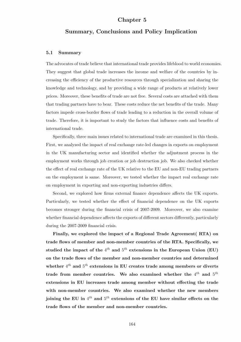
Chapter 5

Summary, Conclusions and Policy Implication

5.1 Summary

The advocates of trade believe that international trade provides lifeblood to world economies.

They suggest that global trade increases the income and welfare of the countries by in-

creasing the efficiency of the productive resources through specialization and sharing the

knowledge and technology, and by providing a wide range of products at relatively lower

prices. Moreover, these benefits of trade are not free. Several costs are attached with them

that trading partners have to bear. These costs reduce the net benefits of the trade. Many

factors impede cross-border flows of trade leading to a reduction in the overall volume of

trade. Therefore, it is important to study the factors that influence costs and benefits of

international trade.

Specifically, three main issues related to international trade are examined in this thesis.

First, we analyzed the impact of real exchange rate-led changes in exports on employment

in the UK manufacturing sector and identified whether the adjustment process in the

employment works through job creation or job destruction job. We also checked whether

the effect of real exchange rate of the UK relative to the EU and non-EU trading partners

on the employment is same. Moreover, we tested whether the impact real exchange rate

on employment in exporting and non-exporting industries differs.

Second, we explored how firms external finance dependence affects the UK exports.

Particularly, we tested whether the effect of financial dependence on the UK exports

becomes stronger during the financial crisis of 2007-2009. Moreover, we also examine

whether financial dependence affects the exports of different sectors differently, particularly

during the 2007-2009 financial crisis.

Finally, we explored the impact of a Regional Trade Agreement( RTA) on

trade flows of member and non-member countries of the RTA. Specifically, we

studied the impact of the 4th and 5th extensions in the European Union (EU)

on the trade flows of the member and non-member countries and determined

whether 4th and 5th extensions in EU creates trade among members or diverts

trade from member countries. We also examined whether the 4th and 5th

extensions in EU increases trade among member without effecting the trade

with non-member countries. We also examined whether the new members

joining the EU in 4th and 5th extensions of the EU have similar effects on the

trade flows of the member and non-member countries.

164

In Chapter 2, the GMM method was used to estimate the dynamics of employment in

the UK manufacturing sector arising from a shock to the real exchange rate. The findings

of the analysis show that the real exchange rate significantly affects employment in the

UK. Specifically, we show that a rise in UK wage costs relative to its trading partner

leads to a significant reduction in net employment in the UK manufacturing sector. This

tendency of a reduction in employment is more pronounced for industries that export

relatively more.

Chapter 2 shows that adjustments in net employment to a shock in competitiveness

mainly occurred due to job creation. Our results also show that the adjustment is not

significantly affected by job destruction. Moreover, Chapter 2 reports that smaller firms

contribute more towards job creation and slightly less towards job destruction than larger

firms. Furthermore, the size of labor adjustment in UK manufacturing sector in response

to real exchange rate led fluctuations in competitiveness of the UK with European and

non-European countries differs.

Moreover, the findings of Chapter 2 show that fluctuations in real exchange rate may

not affect net employment in non-exporting firms. However, an increase in real exchange

rate significantly reduces net employment in exporting firms.

In Chapter 3 OLS with dummies to control sector-time, country-time and

country-sector fixed effect and IV techniques have been used to analyze the

impact of the 2007-2009 global financial crisis on UK trade with its 25 major

trading partners. The findings of this chapter show that credit conditions are

an important channel through which financial turmoil affects the UK exports.

Specifically, the results indicate that with higher lending rates and tighter

credit market conditions the UK exported less during the 2007-2009 financial

crisis. Moreover, these negative effects become stronger for sectors with lim-

ited access to buyer-supplier trade credit, with lesser collateralizable assets,

with higher dependency on external financing and with lower values of the

leverage.

Chapter 3 also shows that adverse credit conditions affect the supply and

demand side of exports significantly and play a significant role in determining

the supply and the demand of the UK exports. Moreover, it shows that the

demand for exports is primarily driven by the importing country’s GDP, cap-

ital labor ratio, interest rates and the credit to private sector. Whereas UK’s

GDP, capital labor ratio, interest rates and availability and the accessibility of

the external funds significantly determine the supply of UK exports. The ob-

servation that financial markets disruptions reduce UK exports is robust and

does not change with the change in proxy used for the cost of capital and the

165

change in measures used for the financial dependency of a sector on external

resources.

In Chapter 4, we use correctly specified fixed effect gravity model to es-

timate the effects of the 4th and 5th extensions in the European Union (EU)

on the trade flows of member and non member countries. The findings show

that the effects of 4th and 5th extensions in the EU on trade flows are mixed.

Only in two out of ten commodity groups does the EU create trade among

members without affecting the EU trade with non-member countries while in

all other product categories the 4th and 5th extensions in the EU diverts trade

from member countries to rest of the world. In general, Chapter 4 shows that

the EU boosts the intra-bloc trade at the cost of reducing the trade with extra

bloc trading partners. However, in case of “Minerals Fuels, Lubricants and

Related material” and “Machinery and Transport Equipments” commodity

groups, 4th and 5th extensions in EU results in increasing the trade with mem-

ber countries without affecting the trade with non-member countries. In these

two commodity groups 4th and 5th extensions in the EU increase trade with

non-member countries along with increasing the trade with member countries.

These finding make sense because the EU member countries are oil deficient

countries and they meet their energy and fuel demand by importing fuels and

related products from the non-member countries. Moreover, the EU coun-

tries import raw material or the intermediate goods, process them and then

re-exports the final products.

Furthermore the findings of the chapter show that trade creation and trade

diversion effects of the extensions in the EU vary across the extensions, across

the new members joining the EU in these extensions and across the commodity

groups. This finding make sense because the extensions of the EU vary across

time, in the number and the sizes of the countries joining the EU in these

extensions and in variations in the nature of the products included in different

commodity groups.

Finally, in this chapter, we show that the major share of “food and live animal” prod-

ucts is imported from non-member countries and the EU is the net importer of the food

and agriculture products. Furthermore, the analysis shows that “machinery and trans-

port equipments”, “chemical and related products” and the “manufactured goods chiefly

classified by material” are the major contributors in the excellent export performance of

the EU.

166

5.2 Conclusions

The fluctuations in real exchange rates significantly affect the employment in UK manu-

facturing sector and the adjustment in net employment to a shock in the real exchange

rate mainly works through job creation. The UK labor market responds to shocks sig-

nificantly and induces the employment smoothing accordingly. That is, the workers fired

in bad times will be rehired in good times. So, employment will be high in good times

and unemployment will be high in bad times. Moreover, the employment in small firms

is more sensitive to fluctuations in competitiveness than large firms. The employment in

exporting and in non-exporting firms behave differently in response to the change in the

real exchange rate. Furthermore, the insiders (employed) benefit from the higher wages

while outsiders (unemployed) bear the cost of the job reallocation process.

Overall, the financial crisis of 2007-2009 has significantly affected the UK exports.

Specifically, the exports of the sectors that depend more on external finance, have limited

access to buyer-supplier trade credit and have lesser tangible assets, were severely damaged

during the crisis. Adverse credit conditions are important channel through which financial

turmoil transmit its effect to international trade flows of the UK. Rises in cost of the capital

significantly reduce the UK exports and this reduction even became more intensive during

the financial crisis of 2007-2009.

On the whole our finding suggest that trade creation and trade diversion

effects of the extensions in the EU vary across the extensions, across the com-

modity groups, and across the new members joining the EU in fourth and fifth

extensions of the EU. These findings indicate that 5th extension has resulted

in trade creation but 4th extension has resulted in trade diversion. In some

commodity groups the EU increases trade among member countries while in

other commodity groups the EU diverts trade from member countries to non-

member countries. Specifically, the EU results in trade creation in 8 out of 10

commodity groups. The EU is net importer of the food and agricultural prod-

ucts. Moreover, the “machinery and transport equipments”, “chemical and

related products” and the “manufactured goods chiefly classified by material”

are major exports of the EU.

5.3 Policy Implications

Our findings show that the loss in international competitiveness significantly decreases

the employment in the UK manufacturing sector. Particularly, we observe that decrease

in the international competitiveness leads to a significant reduction in employment in the

exporting industries. These findings are useful in policing making as they suggest that

167

there is a need to take policy measures that encourage job creations in non-trading indus-

tries, improve labor productivity and encourage domestic consumption-led growth. These

policy measures will be helpful in reducing the negative effects of the loss of international

competitiveness on employment and strengthens the labor markets to absorb the negative

shocks to international trade.

Our findings also suggest that policy interventions that reduce the cost of capital

will be really helpful in reducing substantially the detrimental effects of severe financial

disruptions on international trade flows. Particularly, ensuring the provision of the credit

at affordable rate to financially constrained firms during the crisis will enhance the exports.

Our findings suggest that the EU countries should take measures to improve

the productivity of the members countries so that they fulfill export order

from the members and well from the non-member countries. By improving

the productivity and the productive capacity of the member countries the EU

can reduce at least the exports diversion caused by the new members joining

the EU in the extensions of the EU.

168

Appendix A: Trade Competitiveness and Employment: JobCreation or Job Destruction ?

Table A.1: Job Creation in Manufacturing Sector of the UK (Exporting In-dustries)


L.Job Creation 0.163 0.131 0.148 0.064 0.321**(0.165) (0.185) (0.181) (0.149) (0.15)

L. Job Destruction -0.229 -0.193 -0.160 -0.123 -0.208(0.193) (0.222) (0.209) (0.194) (0.304)

Average Wage -0.102* -0.094** -0.069* -0.083* -0.165***(0.061) (0.042) (0.039) (0.049) (0.061)

GDP Growth .003*** 0.003*** 0.003*** .002** 0.002*(0.001) (0.001) (0.001) (0.001) (0.001)

Sales Growth 0.001 0.001 0.001 0.002 -0.001(0.004) (0.004) (0.004) (0.004) (0.005)

Size -0.003 -0.159 -0.105 -0.026 0.026(0.039) (0.089) (0.085) (0.058) (0.054)

Competitiveness -0.174*(32 Partners) (0.104)Competitiveness -0.159 -0.056 0.060(EU Partners) (0.116) (0.15) (0.349)Competitiveness -0.105*** -0.097** -0.068(non-EU Partners) (0.032) (0.046) (0.102)Competitiveness 1.983(Interaction) (3.318)Constant 0.072 0.072 0.066 0.072*** 0.072***

(0.02) (0.019) (0.017) (0.02) (0.025)



169

Table A.2: Job Destruction in Manufacturing Sector of the UK (ExportingIndustries)


L.Job Creation 0.078 0.089 0.071 0.087 0.113(0.155) (0.128) (0.125) (0.128) (0.139)

L. Job Destruction 0.401*** 0.392*** 0.391*** .404*** .476***(0.133) (0.134) (0.125) (0.124) (0.148)

Average Wage -0.178* -0.181* -0.191** -0.176** -0.169**(0.101) (0.098) (0.092) (0.088) (0.083)

GDP Growth -0.004*** -0.004*** -0.004*** -0.004*** -0.005***(0.002) (0.001) (0.002) (0.002) (0.002)

Sales Growth 0.005 0.005 0.005 0.005 0.005(0.005) (0.005) (0.005) (0.005) (0.005)

Size -0.062 -0.044 -0.043 -0.046 -0.041(0.082) (0.076) (0.076) (0.073) (0.087)

Competitiveness 0.071(32 Partners) (0.0732)Competitiveness 0.087 0.011 0.276(EU Partners) (0.083) (0.125) (0.323)Competitiveness 0.022 -0.015 -0.045(non-EU Partners) (0.041) (0.064) (0.087)Competitiveness 2.200(Interaction) (3.165)Constant 0.094*** 0.091 .093*** .090*** 0.082***

(0.034) (0.032) (0.032) (0.031) (0.03)



170

Table A.3: Gross Job Flows in Manufacturing Sector of the UK (ExportingIndustries)


L.Job Creation 0.125 0.107 0.070 0.107 0.129(0.273) (0.253) (0.267) (0.25) (0.272)

L. Job Destruction 0.149 0.127 0.163 0.160 0.245(0.226) (0.231) (0.211) (0.203) (0.313)

Average Wage -0.398*** -0.411*** -0.366*** -0.393*** -0.371***(0.091) (0.08) (0.106) (0.083) (0.093)

GDP Growth -0.003* -0.003** -0.003* -0.003** -0.003**(0.003) (0.002) (0.002) (0.002)) (0.002)

Sales Growth 0.005 0.005 0.005 0.005 0.004(0.004) (0.004) (0.005) (0.004) (0.004)

Size -0.035 -0.030 -0.032 -0.030 -0.027(0.155) (0.148) (0.152) (0.145) (0.135)

Competitiveness -0.091(32 Partners) (0.103)Competitiveness -0.102 -0.029 0.165(EU Partners) (0.116) (0.148) (0.495)Competitiveness -0.050 -0.063 -0.100(non-EU Partners) (0.044) (0.063) (0.09)Competitiveness 2.479(Interaction) (5.348)Constant 0.195*** .199*** .191*** 0.194*** 0.182***

(0.031) (0.03) (0.031) (0.03) (0.402)



171

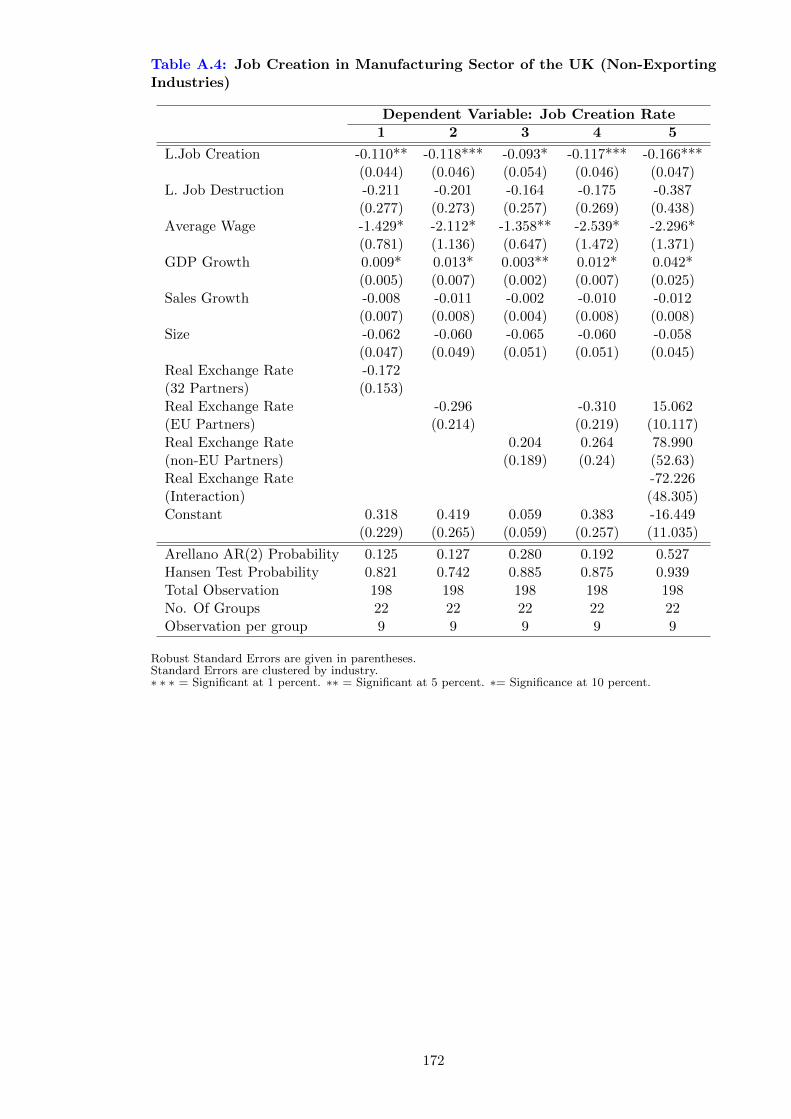
Table A.4: Job Creation in Manufacturing Sector of the UK (Non-ExportingIndustries)


L.Job Creation -0.110** -0.118*** -0.093* -0.117*** -0.166***(0.044) (0.046) (0.054) (0.046) (0.047)

L. Job Destruction -0.211 -0.201 -0.164 -0.175 -0.387(0.277) (0.273) (0.257) (0.269) (0.438)

Average Wage -1.429* -2.112* -1.358** -2.539* -2.296*(0.781) (1.136) (0.647) (1.472) (1.371)

GDP Growth 0.009* 0.013* 0.003** 0.012* 0.042*(0.005) (0.007) (0.002) (0.007) (0.025)

Sales Growth -0.008 -0.011 -0.002 -0.010 -0.012(0.007) (0.008) (0.004) (0.008) (0.008)

Size -0.062 -0.060 -0.065 -0.060 -0.058(0.047) (0.049) (0.051) (0.051) (0.045)


(0.229) (0.265) (0.059) (0.257) (11.035)



172

Table A.5: Job Destruction in Manufacturing Sector of the UK (Non-Exporting Industries)


L.Job Creation -0.019 -0.019 -0.018 -0.018 0.008(0.059) (0.056) (0.058) (0.06) (0.086)

L. Job Destruction 0.289* 0.288* 0.276* 0.282* 0.336*(0.151) (0.154) (0.157) (0.161) (0.154)

Average Wage 0.726 0.823 0.185 0.355 0.363(0.801) (0.922) (0.9) (1.091) (1.105)

GDP Growth -0.003 -0.002 -0.001 -0.003 (-0.015)*(0.005) (0.005) (0.005) (0.005) (0.009)

Sales Growth 0.003 0.002 0.002 0.003 0.007(0.009) (0.009) (0.01) (0.009) (0.01)

Size 0.116 0.114 0.102 0.110 0.104(0.108) (0.103) (0.105) (0.101) (0.099)

Real Exchange Rate 0.069(32 Partners) (0.098)Real Exchange Rate 0.046 0.046 -5.362(EU Partners) (0.126) (0.127) (3.619)Real Exchange Rate 0.176 0.177 -27.724(non-EU Partners) (0.192) (0.197) (18.508)Real Exchange Rate 25.545(Interaction) (16.945)Constant -0.062 -0.026 -0.001 -0.053 5.887

(0.133) (0.147) (0.057) (0.144) (3.982)



173

Table A.6: Gross Job Flows in Manufacturing Sector of the UK (Non-Exporting Industries)


L.Job Creation -0.331 -0.289 -0.405 -0.293 -0.301(0.254) (0.259) (0.286) (0.26) (0.27)

L. Job Destruction 0.220* 0.285* 0.230* 0.315* 0.299**(0.126) (0.158) (0.117) (0.165) (0.139)

GDP Growth 0.005 0.008 -0.002 0.008 0.010(0.005) (0.006) (0.007) (0.006) (0.013)

Sales Growth -0.002 -0.004 0.003 -0.003 -0.003(0.008) (0.009) (0.007) (0.008) (0.009)

Size 0.262 0.280 0.332 0.307 0.307(0.323) (0.342) (0.401) (0.361) (0.362)


(0.276) (0.289) (0.091) (0.279) (5.917)



174

Table A.7: Manufacturing Industry Classification (UK SIC 2003)

Code Industry

15 Food products and Beverages16 Tobacco products17 Textiles18 Wearing apparel; dressing & dyeing of fur19 Tanning & dressing of leather & leather products20 Wood and of products of wood and cork except furniture21 Pulp, paper and paper products22 Publishing, printing and reproduction of recorded media23 Coke refined petroleum products24 Chemicals and chemical products25 Rubber and plastic products26 Other non-metallic mineral products27 Basic metals28 Fabricated metal products, except machinery and equipment29 Machinery and equipment not elsewhere classified30 Office machinery and computers31 Electrical machinery and apparatus not elsewhere classified32 Radio, television and communication equipment and apparatus33 Medical, precision and optical instruments, watches and clocks34 Motor vehicles, trailers and semi-trailers35 Other transport equipment36 Furniture; manufacturing not elsewhere classified

175

Figure 16: Average Share of Export in Total Sale in UK Manufacturing In-dustries

0

5

10

15

20

25

30

35

Figure 17: Employment in Manufacturing sector of the UK

0

50000

100000

150000

200000

250000

300000

350000

400000

450000

1999 2000 2001 2002 2003 2004 2005 2006 2007 2008 2009

Employment (All Industries)

Employment (Exporting Industries)

Employment (Non-Exporting Industries)

176

Figure 18: Average UK’s Real Exchange Rate with top 5 Trading Partnersfrom 1999 to 2010

0

0.02

0.04

0.06

0.08

0.1

0.12

0.14

0.16

0.18

USA

Germany

Ireland

Netherlands

Italy

Trade weighted real exchange rate average for each partner is calculated using

trade weighted real exchange rate values from 1999 to 2010.

Figure 19: UK Manufacturing Exports by Industry from 1999 to 2010

12

14

16

18

12

14

16

18

12

14

16

18

12

14

16

18

12

14

16

18

2000 2005 2010 2000 2005 2010 2000 2005 2010

2000 2005 2010 2000 2005 2010

15 16 17 18 19

20 21 22 23 24

25 26 27 28 29

30 31 32 33 34

35 36

lexp

ort

YearSee Table A.7 for Industry Codes Explanation

177

Appendix B: Financial Turmoil, External Finance and UKExports

Table B.1: Trade Credit and Overnight Interbank Rate


IBrate * TCRED 0.572*** 0.444** 0.463***(0.141) (0.146) (0.148)

D Crisis * IBrate * TCRED 0.179*** 0.138**(0.054) (0.057)


UK Interest Rate -0.050** -0.058*** -0.061***(0.016) (0.017) (0.018)


UK GDP 4.107 3.620 4.300(2.907) (2.952) (3.484)

Partner GDP 1.002*** 1.002*** 1.070***(0.065) (0.065) (0.027)

UK K/L Ratio -1.902** -1.903** -2.366***(0.680) (0.678) (0.695)

Partner K/L Ratio 0.547*** 0.546*** 0.618***(0.090) (0.090) (0.036)

N 13916 13916 12566r2 0.939 0.939 0.935



* p < 0.10, ** p < 0.05, *** p < 0.01

178

Table B.2: Tangible Assets and Overnight Interbank Rate


IBrate * TANG 0.022 -0.013 -0.006(0.040) (0.044) (0.044)

D Crisis * IBrate * TANG 0.048*** 0.040**(0.013) (0.014)


UK Interest Rate 0.004 -0.002 -0.007(0.017) (0.017) (0.021)


UK GDP 5.179* 4.312 5.001(2.887) (2.945) (3.281)

Partner GDP 1.002*** 1.002*** 1.070***(0.064) (0.064) (0.026)

UK K/L Ratio -1.865** -1.861** -2.326***(0.675) (0.674) (0.691)

Partner K/L Ratio 0.546*** 0.545*** 0.618***(0.088) (0.088) (0.035)

N 13916 13916 12566r2 0.939 0.939 0.935



* p < 0.10, ** p < 0.05, *** p < 0.01

179

Table B.3: Leverage and Overnight Interbank Rate


IBrate * Leverage 0.154*** 0.123** 0.131**(0.049) (0.054) (0.051)

D Crisis * IBrate * Leverage 0.050*** 0.041**(0.014) (0.015)


UK Interest Rate -0.049** -0.059*** -0.064**(0.020) (0.019) (0.023)


UK GDP 4.466 3.849 4.497(2.938) (2.975) (3.509)

Partner GDP 1.002*** 1.002*** 1.070***(0.065) (0.065) (0.026)

UK K/L Ratio -1.889** -1.882** -2.348***(0.678) (0.677) (0.692)

Partner K/L Ratio 0.547*** 0.546*** 0.618***(0.090) (0.090) (0.035)

N 13916 13916 12566r2 0.939 0.939 0.935



* p < 0.10, ** p < 0.05, *** p < 0.01

180

Tab

leB

.4:

Su

mm

ary

Sta

tist

ics

Peri

od

Vari

ab

leO

bs.

Mean

Std

.D

ev.

Min

Max

Exp

orts

1594

255

.52

133.

270.0

002

2629.1

3U

Kle

nd

ing

rate

1600

04.

340.

483.5

05.2

5B

efor

eU

Kin

terb

ank

rate

1600

04.

340.

483.5

05.2

5th

eU

KG

DP

1600

019

3125

0.00

8455

1.08

1800000.0

02100000.0

0C

risi

sU

KK

/L16

000

1908

1.73

2667

.50

15619.5

923439.2

3P

artn

erle

nd

ing

rate

1172

06.

202.

921.6

018.3

0P

artn

erin

terb

ank

rate

1083

06.

299.

540.1

060.0

0P

artn

erG

DP

1600

015

0067

6.00

2533

183.

003.9

813000000.0

0P

artn

erK

/L12

800

3190

0000

.00

1380

0000

0.00

860.4

2719000000.0

0P

artn

erC

laim

son

Pvt.

Sec

tor

1466

024

8000

00.0

010

2000

000.

0019772.2

0560000000.0

0

Exp

orts

5452

64.2

912

9.60

0.0

01

1185.6

8U

Kle

nd

ing

rate

5500

4.69

1.40

1.0

05.7

5D

uri

ng

UK

inte

rban

kra

te55

004.

691.

401.0

05.7

5th

eU

KG

DP

5500

2090

909.

0028

750.

592000000.0

02100000.0

0C

risi

sU

KK

/L55

0022

102.

6914

33.9

418215.0

423439.2

3P

artn

erle

nd

ing

rate

3370

6.85

3.07

1.8

017.1

0P

artn

erin

terb

ank

rate

3740

5.69

5.62

0.1

327.0

0P

artn

erG

DP

5500

1725

639.

0028

2186

8.00

6.9

013000000.0

0P

artn

erK

/L44

0036

1000

00.0

015

5000

000.

001162.5

2721000000.0

0P

artn

erC

laim

son

Pvt.

Sec

tor

4890

2760

0000

.00

1030

0000

0.00

97720.9

0510000000.0

0

Exp

orts

7629

67.1

513

5.43

0.0

01

1300.8

9U

Kle

nd

ing

rate

7750

0.50

0.00

0.5

00.5

0A

fter

UK

inte

rban

kra

te77

500.

500.

000.5

00.5

0th

eU

KG

DP

5500

2000

000.

000.

002000000.0

02000000.0

0C

risi

sU

KK

/L55

0019

859.

4615

01.2

818215.0

421229.8

1P

artn

erle

nd

ing

rate

4350

5.47

3.18

1.5

016.1

0P

artn

erin

terb

ank

rate

5210

3.32

4.15

0.1

325.0

0P

artn

erG

DP

5380

1814

419.

0029

6592

6.00

8.2

613000000.0

0P

artn

erK

/L44

0033

6000

00.0

014

5000

000.

001179.9

8682000000.0

0P

artn

erC

laim

son

Pvt.

Sec

tor

6330

2810

0000

.00

9900

0000

.00

174177.0

0503000000.0

0

Inte

rest

rate

sare

inp

erce

nta

ges

and

all

oth

erva

riable

sare

inm

illion.

Cri

sis

Per

iod

isfr

om

May

2007

toF

ebru

ary

2009

(Wis

nie

wsk

iand

Lam

be,

2011).

181

Figure 20: Monthly Share Price Index of the UK

0

20

40

60

80

100

120

140 2002 Jan

2002 Jul

2003 Jan

2003 Jul

2004 Jan

2004 Jul

2005 Jan

2005 Jul

2006 Jan

2006 Jul

2007 Jan

2007 Jul

2008 Jan

2008 Jul

2009 Jan

2009 Jul

2010 Jan

2010 Jul

2011 Jan

2011 July

a: Monthly Share Price index of the UK from Jan 2002 to Sep 2011

Share Price index

0

20

40

60

80

100

120

140

2007 May

2007 Jul

2007 Sep

2007 Nov

2008 Jan

2008 Mar

2008 May

2008 Jul

2008 Sep

2008 Nov

2009 Jan

b: Monthly Share Price index of the UK from May 2007 to Feb 2009

Share Price index

182

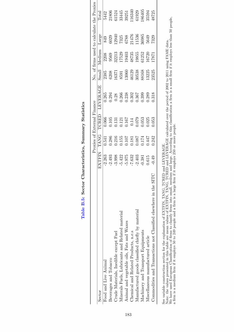
Tab

leB

.5:

Secto

rC

hara

cte

rist

ics,

Su

mm

ary

Sta

tist

ics

Pro

xie

sof

Exte

rnal

Fin

an

ceN

o.

of

firm

su

sed

toca

lcu

late

the

Pro

xie

s

Sec

tor

EX

TF

INT

AN

GT

CR

ED

LE

VE

RA

GE

Sm

all

Med

ium

Larg

eT

ota

l

Food

and

Liv

eA

nim

al-2

.263

0.54

10.

066

0.2

65

2385

2208

849

5442

Bev

erag

esan

dT

obac

co-2

.493

0.28

60.

105

0.2

94

6208

9569

6029

21806

Cru

de

Mat

eria

ls,

Ined

ible

exce

pt

Fu

el-3

.998

0.21

60.

131

0.2

816371

32213

12940

61524

Min

eral

sF

uel

s,L

ub

rica

nts

and

Rel

ated

mat

eria

l-5

.422

0.15

50.

121

0.2

66

8591

17529

7325

33445

An

imal

and

vege

tab

leoi

ls,

Fat

san

dW

axes

-5.9

750.

107

0.16

70.2

38

13060

19403

6788

39251

Ch

emic

alan

dR

elat

edP

rod

uct

s,n

.e.s

-7.6

320.

181

0.14

0.3

02

46129

48735

21476

116340

Man

ufa

ctu

red

good

scl

assi

fied

chie

fly

by

mat

eria

l-2

.403

0.08

70.

079

0.3

67

30538

19855

11536

61929

Mac

hin

ery

and

Tra

nsp

ort

Equ

ipm

ents

-0.3

810.

174

0.05

30.3

99

88168

61252

36985

186405

Mis

cell

aneo

us

man

ufa

ctu

red

arti

cle

0.61

50.

447

0.02

50.2

89

13225

16720

5649

35594

Com

mod

itie

san

dT

ran

sact

ion

sn

otC

lass

ified

else

wh

ere

inth

eS

ITC

-0.4

90.

242

0.05

30.3

18

23525

17871

7329

48725

See

vari

able

const

ruct

ion

sect

ion

for

the

expla

nati

on

of

EX

TF

IN,

TA

NG

,T

CR

ED

and

LE

VE

RA

GE

.N

ote

:th

eva

lues

pre

sente

din

this

table

are

mea

nva

lues

of

EX

TF

IN,

TA

NG

,T

CR

ED

and

LE

VE

RA

GE

calc

ula

ted

over

the

per

iod

of

2002

to2011

usi

ng

FA

ME

data

.W

ehav

euse

dE

uro

pea

nC

lass

ifica

tion

of

firm

sto

class

ify

firm

sin

tosm

all,

med

ium

and

larg

e.A

ccord

ing

toth

iscl

ass

ifica

tion

afirm

isa

small

firm

ifit

emplo

ys

less

than

50

peo

ple

,a

firm

isa

med

ium

firm

ifit

emplo

ys

50

to249

peo

ple

and

afirm

isa

larg

efirm

ifit

emplo

ys

250

or

more

peo

ple

.

183

Table B.6: Standard International Trade Classification, Revision 3

SITC Code Explanation

SITC-0 Food and Live AnimalSITC-1 Beverages and TobaccoSITC-2 Crude Materials, Inedible except FuelSITC-3 Minerals Fuels, Lubricants and Related materialSITC-4 Animal and vegetable oils, Fats and WaxesSITC-5 Chemical and Related Products, n.e.sSITC-6 Manufactured goods classified chiefly by materialSITC-7 Machinery and Transport EquipmentsSITC-8 Miscellaneous manufactured articleSITC-9 Commodities and Transactions not Classified elsewhere in the SITC

184

Appendix C: Trade Creation and Diversion Effects ofEuropean Union

Table C.1: Trade agreements of Europe

Country EEA ECCU ECFTA EA CEFTA MCA EMA

Algeria - - - - - 1976 2002Austria 1994 1995 1973 - - - -Belgium 1994 1957 1957 - - - -Bulgaria - - - 1993 1999 - -Croatia - - 2002 - 2003 - -Cyprus 2004 2004 1973 - - - -The Czech Rep. 2004 2004 - 1992 1993 - -Denmark 1994 1973 1973 - - - -Egypt - - - - - 1977 2004Estonia 2004 2004 - 1995 - - -Finland 1994 1995 1973 - - - -France 1994 1957 1957 - - - -Germany 1994 1957 1957 - - - -Greece 1994 1981 1981 - - - -Hungary 2004 2004 - 1992 1993 - -Iceland 1994 - 1973 - - - -Ireland 1994 1973 1973 - - - -Israel - - - - - - 2002Italy 1994 1957 1957 - - - -Jordan - - - - - 1977 2002Latvia 2004 2004 - 1995 - - -Lebanon - - - - - 1977 2003Lithuania 2004 2004 - 1995 - - -Luxembourg 1994 1957 1957 - - - -FYR Macedonia - - 2001 - - - -Malta 1994 2004 1971 - - - -Morocco - - - - - - 2000Netherlands 1994 1957 1957 - - - -Norway 1994 - 1973 - - - -Palestine - - - - - - 1997Poland 2004 2004 - 1992 1993 - -Portugal 1994 1986 1973 - - - -Romania - - - 1993 1997 - -The Slovakia 2004 2004 - 1992 1993 - -Slovenia 2004 2004 - 1997 1996 - -Spain 1994 1986 1986 - - - -Sweden 1994 1995 1973 - - - -Switzerland 1994 - 1973 - - - -Syria - - - - - 1977 -Tunisia - - - - - - 1998Turkey - 1996 1963 - - - -The UK 1994 1973 1973 - - - -

source; Kandogan (2005)

EEA= European Economic Area. ECCU= European Community’s Customs Union.

ECFTA= European Free Trade Area. EA= Europe Agreements. EMA= Euro-Mediterranean Agreements

CEFTA= Central European Free Trade Area. MCA= Mediterranean Cooperation Agreements

185

Tab

leC

.2:

Com

mod

ity

Level

Exp

ort

sof

the

EU

befo

re5th

Exte

nsi

on

inth

eE

U

Dep

end

ent

Var

iab

le:

log(

Exp

orts

)S

ITC

-0S

ITC

-1S

ITC

-2S

ITC

-3S

ITC

-4S

ITC

-5S

ITC

-6S

ITC

-7S

ITC

-8S

ITC

-9

Yi

0.76

3***

1.38

2***

0.59

3*1.

217*

**3.

372*

**2.

120*

**1.

483*

**1.8

38***

1.2

01***

0.9

83

(0.2

12)

(0.3

66)

(0.3

07)

(0.4

30)

(0.6

11)

(0.2

22)

(0.2

39)

(0.2

20)

(0.2

05)

(0.6

90)

Yj

-0.0

100.

445*

0.11

20.

737*

**0.

045

0.17

6***

0.29

2*0.3

53**

0.2

18*

0.2

69**

(0.1

45)

(0.2

32)

(0.1

14)

(0.1

66)

(0.1

95)

(0.0

67)

(0.1

66)

(0.1

46)

(0.1

16)

(0.1

17)

dij

-1.5

36**

*-1

.590

***

-1.6

06**

*-2

.881

***

-1.4

98**

*-1

.828

***

-1.7

40**

*-1

.721***

-1.5

57***

-1.2

33***

(0.1

40)

(0.1

53)

(0.1

20)

(0.1

75)

(0.1

79)

(0.1

23)

(0.1

06)

(0.1

09)

(0.1

34)

(0.1

60)

SIM

0.01

9-0

.187

0.08

40.

065

0.02

3-0

.076

-0.0

52-0

.080

-0.1

53*

-0.1

69

(0.1

08)

(0.1

34)

(0.0

97)

(0.1

50)

(0.1

61)

(0.0

64)

(0.0

99)

(0.0

82)

(0.0

88)

(0.1

36)

∆e ij

0.18

3***

0.13

0***

0.14

4***

0.13

4***

0.14

0***

0.19

5***

0.21

4***

0.1

79***

0.1

70***

0.1

25***

(0.0

33)

(0.0

40)

(0.0

35)

(0.0

47)

(0.0

38)

(0.0

40)

(0.0

43)

(0.0

34)

(0.0

25)

(0.0

31)

Ri

0.54

3***

0.31

8***

0.46

1***

0.50

3***

0.31

6***

0.75

4***

0.60

7***

0.6

31***

0.6

15***

-0.3

74***

(0.0

57)

(0.0

72)

(0.0

65)

(0.0

90)

(0.1

09)

(0.0

42)

(0.0

42)

(0.0

42)

(0.0

38)

(0.0

88)

Rj

0.06

5**

0.04

70.

077*

*0.

065

0.04

30.

036

0.01

50.0

95***

0.0

57**

0.0

26

(0.0

28)

(0.0

45)

(0.0

36)

(0.0

51)

(0.0

41)

(0.0

25)

(0.0

32)

(0.0

25)

(0.0

28)

(0.0

39)

RF

0.01

6-0

.177

**0.

065

-0.0

05-0

.050

-0.0

080.

018

0.0

13

-0.0

93

-0.1

14

(0.0

71)

(0.0

89)

(0.0

63)

(0.1

04)

(0.1

12)

(0.0

49)

(0.0

57)

(0.0

55)

(0.0

58)

(0.1

05)

COL

0.83

1***

0.67

5***

0.75

5***

0.59

8**

0.60

6***

0.93

0***

0.91

7***

1.0

85***

1.2

31***

0.8

21***

(0.1

69)

(0.1

81)

(0.1

44)

(0.2

40)

(0.2

09)

(0.1

58)

(0.1

57)

(0.1

72)

(0.1

85)

(0.1

72)

CL

0.91

6***

0.63

5***

0.68

0***

0.30

80.

606*

*0.

664*

**0.

674*

**0.6

25***

0.9

02***

0.9

64***

(0.1

72)

(0.1

74)

(0.1

51)

(0.2

41)

(0.2

40)

(0.1

44)

(0.1

52)

(0.1

66)

(0.1

61)

(0.2

01)

CB

0.84

9***

0.58

6***

0.70

6***

1.19

2***

1.16

8***

0.42

7**

0.23

90.0

29

0.1

80

0.5

51***

(0.1

84)

(0.2

26)

(0.1

86)

(0.2

26)

(0.2

09)

(0.1

88)

(0.1

59)

(0.2

00)

(0.2

15)

(0.2

12)

N16

879

1360

114

424

1013

278

9920

189

2104

621607

20307

9209

r2o

0.71

10.

645

0.73

20.

607

0.56

80.

787

0.81

50.8

10

0.8

20

0.6

40

Robust

Sta

ndard

erro

rsin

pare

nth

eses

,Sta

ndard

erro

rsare

clust

ered

by

Part

ner

Tim

e,R

eport

er,

Part

ner

and

Sec

tor

fixed

effec

tsare

contr

olled

*p<

0.1

,**p<

0.0

5,

***p<

0.0

1

See

Table

C.6

inth

eA

pp

endix

Cfo

rSIT

CC

ode

Expla

nati

on.

186

Tab

leC

.3:

Com

mod

ity

Level

Exp

ort

sof

the

EU

befo

re4th

Exte

nsi

on

inth

eE

U

Dep

end

ent

Var

iab

le:

log(

Exp

orts

)S

ITC

-0S

ITC

-1S

ITC

-2S

ITC

-3S

ITC

-4S

ITC

-5S

ITC

-6S

ITC

-7S

ITC

-8S

ITC

-9

Yi

1.30

7**

-0.3

970.

168

-0.8

782.

357

1.95

4***

1.07

0**

1.9

91***

0.6

27

18.9

35***

(0.5

93)

(0.5

12)

(0.4

94)

(1.5

22)

(1.5

49)

(0.4

22)

(0.5

00)

(0.5

20)

(0.4

33)

(1.4

31)

Yj

-0.0

150.

718*

*0.

515*

**1.

131*

*0.

169

0.23

1*0.

448*

0.3

90*

0.4

06**

0.5

62***

(0.4

50)

(0.3

55)

(0.1

65)

(0.5

49)

(0.2

99)

(0.1

32)

(0.2

37)

(0.2

30)

(0.1

82)

(0.2

13)

dij

-1.2

28**

*-1

.544

***

-1.3

39**

*-2

.888

***

-1.7

06**

*-1

.751

***

-1.6

58**

*-1

.521***

-1.2

04***

-1.0

63***

(0.1

32)

(0.1

91)

(0.1

30)

(0.2

62)

(0.1

48)

(0.1

37)

(0.1

38)

(0.1

27)

(0.1

58)

(0.1

87)

SIM

0.07

6-0

.256

-0.0

08-0

.097

0.10

9-0

.007

-0.0

88-0

.011

-0.1

40

0.2

02

(0.1

83)

(0.1

77)

(0.1

16)

(0.2

63)

(0.2

52)

(0.1

02)

(0.1

22)

(0.1

23)

(0.1

12)

(0.1

78)

∆e ij

0.20

8***

0.16

9**

0.08

3**

0.04

70.

116

0.13

1***

0.14

4***

0.1

02**

0.1

66***

0.0

79**

(0.0

49)

(0.0

68)

(0.0

39)

(0.0

99)

(0.0

71)

(0.0

43)

(0.0

51)

(0.0

50)

(0.0

49)

(0.0

33)

Ri

0.24

0***

0.23

3***

0.38

8***

0.14

2-0

.169

0.11

2**

0.18

9***

0.4

54***

0.2

76***

-0.5

15***

(0.0

80)

(0.0

90)

(0.0

78)

(0.1

47)

(0.1

55)

(0.0

53)

(0.0

62)

(0.0

74)

(0.0

60)

(0.1

36)

Rj

-0.0

29-0

.074

*0.

072

0.10

20.

064

0.01

80.

030

0.0

28

0.0

25

-0.0

58*

(0.0

59)

(0.0

44)

(0.0

54)

(0.0

80)

(0.0

81)

(0.0

40)

(0.0

47)

(0.0

39)

(0.0

39)

(0.0

32)

RF

0.04

4-0

.200

*-0

.047

-0.1

13-0

.065

0.02

3-0

.057

-0.0

09

-0.0

59

0.1

72

(0.1

23)

(0.1

21)

(0.0

91)

(0.1

74)

(0.1

68)

(0.0

70)

(0.0

89)

(0.0

95)

(0.0

84)

(0.1

23)

COL

0.89

4***

0.62

4***

0.97

7***

0.81

4***

0.21

41.

024*

**1.

102*

**1.1

44***

1.3

59***

0.7

40***

(0.1

85)

(0.2

05)

(0.1

60)

(0.2

95)

(0.2

69)

(0.1

74)

(0.1

73)

(0.1

80)

(0.1

96)

(0.2

01)

CL

0.79

8***

0.63

6***

0.53

8***

0.22

80.

873*

**0.

635*

**0.

674*

**0.7

44***

1.0

17***

1.2

56***

(0.1

86)

(0.1

95)

(0.1

79)

(0.3

38)

(0.2

89)

(0.1

50)

(0.1

63)

(0.1

77)

(0.1

77)

(0.2

25)

CB

0.72

5***

0.47

3*0.

327*

0.67

7**

0.88

0***

0.06

0-0

.268

-0.1

96

-0.0

69

0.2

14

(0.2

22)

(0.2

54)

(0.1

94)

(0.3

30)

(0.2

78)

(0.2

31)

(0.2

04)

(0.2

49)

(0.2

67)

(0.3

35)

N55

0448

3248

3933

4629

1963

6466

216785

6496

3393

r2o

0.76

40.

721

0.79

00.

671

0.61

20.

838

0.85

90.8

40

0.8

63

0.7

17

Robust

Sta

ndard

erro

rsin

pare

nth

eses

,Sta

ndard

erro

rsare

clust

ered

by

Part

ner

Tim

e,R

eport

er,

Part

ner

and

Sec

tor

fixed

effec

tsare

contr

olled

*p<

0.1

,**p<

0.0

5,

***p<

0.0

1

See

Table

C.6

inth

eA

pp

endix

Cfo

rSIT

CC

ode

Expla

nati

on.

187

Tab

leC

.4:

Com

mod

ity

Level

Imp

ort

sof

the

EU

befo

re5th

Exte

nsi

on

inth

eE

U

Dep

end

ent

Var

iab

le:

log(

Imp

orts

)S

ITC

-0S

ITC

-1S

ITC

-2S

ITC

-3S

ITC

-4S

ITC

-5S

ITC

-6S

ITC

-7S

ITC

-8S

ITC

-9

Yi

1.23

0***

0.84

6*1.

050*

**1.

090*

1.19

9*1.

092*

**0.

787*

**0.6

43**

2.3

29***

2.4

52***

(0.2

59)

(0.4

52)

(0.2

65)

(0.6

30)

(0.6

20)

(0.2

40)

(0.2

32)

(0.3

03)

(0.2

21)

(0.6

76)

Yj

-0.0

25-0

.194

-0.0

400.

482

0.65

40.

026

0.12

80.3

08**

0.1

31

0.1

20

(0.0

84)

(0.1

54)

(0.0

85)

(0.3

51)

(0.4

63)

(0.1

68)

(0.1

00)

(0.1

32)

(0.1

52)

(0.1

29)

dij

-1.5

44**

*-1

.103

***

-1.6

11**

*-2

.351

***

-1.3

04**

*-1

.635

***

-1.6

73**

*-1

.388***

-1.3

69***

-1.5

50***

(0.1

35)

(0.1

54)

(0.1

44)

(0.2

32)

(0.1

62)

(0.1

22)

(0.1

28)

(0.1

35)

(0.1

45)

(0.2

45)

SIM

0.06

7-0

.130

-0.0

61-0

.391

**-0

.364

**0.

012

0.05

70.0

47

-0.1

07

-0.0

48

(0.0

87)

(0.1

25)

(0.0

91)

(0.1

88)

(0.1

85)

(0.0

88)

(0.0

94)

(0.0

94)

(0.0

98)

(0.1

63)

e ij

-0.1

18**

*-0

.113

***

-0.1

28**

*-0

.213

***

-0.0

56-0

.096

***

-0.0

93**

*-0

.124***

-0.0

86***

-0.0

63

(0.0

25)

(0.0

36)

(0.0

26)

(0.0

54)

(0.0

48)

(0.0

24)

(0.0

22)

(0.0

28)

(0.0

30)

(0.0

39)

Ri

0.43

7***

0.55

4***

0.56

8***

0.46

3***

0.38

6***

0.47

8***

0.42

7***

0.4

58***

0.4

52***

0.2

91**

(0.0

48)

(0.0

89)

(0.0

44)

(0.0

92)

(0.1

06)

(0.0

52)

(0.0

40)

(0.0

47)

(0.0

45)

(0.1

18)

Rj

0.17

0***

0.22

7***

0.15

1***

0.28

2***

0.06

00.

210*

**0.

143*

**0.1

85***

0.0

92

0.0

57

(0.0

50)

(0.0

73)

(0.0

44)

(0.0

93)

(0.0

88)

(0.0

47)

(0.0

39)

(0.0

45)

(0.0

59)

(0.0

72)

RF

0.01

6-0

.071

-0.0

19-0

.170

-0.1

64-0

.009

0.00

40.0

47

-0.0

40

-0.0

02

(0.0

66)

(0.0

89)

(0.0

70)

(0.1

24)

(0.1

56)

(0.0

64)

(0.0

71)

(0.0

70)

(0.0

72)

(0.1

20)

COL

0.95

4***

0.49

4**

0.61

6***

0.26

00.

464*

*0.

542*

**0.

609*

**0.6

08***

0.8

94***

1.0

07***

(0.1

98)

(0.2

39)

(0.2

00)

(0.2

49)

(0.2

22)

(0.1

86)

(0.1

63)

(0.1

83)

(0.1

68)

(0.2

77)

CL

0.88

4***

0.81

4***

0.33

7*0.

345

0.20

00.

421*

*0.

644*

**0.6

35***

0.5

32***

0.9

56***

(0.1

69)

(0.2

37)

(0.1

79)

(0.2

53)

(0.2

30)

(0.2

01)

(0.1

53)

(0.1

58)

(0.1

45)

(0.2

46)

CB

0.42

8**

0.49

9**

0.70

2***

1.17

1***

1.32

7***

0.51

1***

0.24

10.4

09**

0.2

98

0.3

97

(0.1

88)

(0.2

44)

(0.1

92)

(0.3

02)

(0.2

49)

(0.1

95)

(0.1

75)

(0.1

72)

(0.1

89)

(0.3

19)

N18

857

9520

1657

166

0759

1713

130

1740

016505

18368

6936

r2o

0.74

20.

620

0.70

30.

658

0.63

00.

810

0.83

60.8

43

0.8

67

0.6

35

Robust

Sta

ndard

erro

rsin

pare

nth

eses

,Sta

ndard

erro

rsare

clust

ered

by

Part

ner

Tim

e,R

eport

er,

Part

ner

and

Sec

tor

fixed

effec

tsare

contr

olled

*p<

0.1

,**p<

0.0

5,

***p<

0.0

1

See

Table

C.6

inth

eA

pp

endix

Cfo

rSIT

CC

ode

Expla

nati

on.

188

Tab

leC

.5:

Com

mod

ity

Level

Imp

ort

sof

the

EU

befo

re4th

Exte

nsi

on

inth

eE

U

Dep

end

ent

Var

iab

le:

log(

Imp

orts

)S

ITC

-0S

ITC

-1S

ITC

-2S

ITC

-3S

ITC

-4S

ITC

-5S

ITC

-6S

ITC

-7S

ITC

-8S

ITC

-9

Yi

0.94

4*1.

214*

*1.

855*

**1.

552

1.14

50.

765*

1.32

5**

1.0

62*

3.6

12***

8.8

64***

(0.4

86)

(0.5

26)

(0.5

54)

(1.1

76)

(0.8

29)

(0.4

62)

(0.5

90)

(0.6

03)

(0.4

65)

(1.7

15)

Yj

0.44

0**

-0.0

97-0

.186

1.56

2**

0.24

60.

240

-0.2

410.4

76

0.2

41

-0.7

74**

(0.1

99)

(0.3

43)

(0.2

22)

(0.7

50)

(0.3

85)

(0.2

43)

(0.2

05)

(0.2

99)

(0.2

66)

(0.3

69)

dij

-1.1

73**

*-0

.556

***

-1.4

87**

*-2

.045

***

-1.3

76**

*-1

.452

***

-1.4

05**

*-1

.211***

-1.1

26***

-1.3

29***

(0.1

54)

(0.2

12)

(0.1

79)

(0.2

57)

(0.2

10)

(0.1

62)

(0.1

37)

(0.1

24)

(0.1

59)

(0.3

27)

SIM

-0.0

60-0

.136

-0.2

79*

-0.5

13*

-0.4

03-0

.126

0.04

90.1

07

-0.2

41*

0.1

68

(0.1

37)

(0.2

63)

(0.1

67)

(0.2

94)

(0.2

76)

(0.1

39)

(0.1

42)

(0.2

01)

(0.1

45)

(0.2

52)

e ij

-0.0

66**

*-0

.063

*-0

.101

***

-0.2

34**

*-0

.009

-0.1

22**

*-0

.051

*-0

.098**

-0.1

08***

0.1

13**

(0.0

23)

(0.0

35)

(0.0

28)

(0.0

81)

(0.0

57)

(0.0

29)

(0.0

29)

(0.0

41)

(0.0

33)

(0.0

51)

Ri

0.15

6**

0.53

4***

0.17

8**

0.53

9***

0.26

5*0.

345*

**0.

374*

**0.3

54***

0.1

71***

0.0

77

(0.0

77)

(0.1

12)

(0.0

76)

(0.2

09)

(0.1

43)

(0.0

79)

(0.0

75)

(0.0

81)

(0.0

57)

(0.1

77)

Rj

0.06

40.

138*

0.13

3***

0.32

9***

0.02

10.

264*

**0.

128*

**0.1

97***

0.2

05***

-0.0

56

(0.0

41)

(0.0

72)

(0.0

42)

(0.1

11)

(0.1

10)

(0.0

56)

(0.0

48)

(0.0

73)

(0.0

62)

(0.1

05)

RF

-0.0

91-0

.164

-0.2

10*

-0.3

07-0

.351

*-0

.130

-0.0

100.1

32

-0.1

43

0.1

48

(0.1

06)

(0.1

98)

(0.1

11)

(0.2

16)

(0.2

13)

(0.1

06)

(0.1

08)

(0.1

62)

(0.1

15)

(0.2

05)

COL

1.07

3***

0.40

80.

723*

**0.

202

0.23

40.

682*

**0.

691*

**0.8

35***

1.0

19***

1.4

39***

(0.1

85)

(0.2

97)

(0.2

03)

(0.2

68)

(0.2

65)

(0.2

04)

(0.1

64)

(0.1

90)

(0.1

59)

(0.2

84)

CL

0.86

9***

0.85

2***

0.19

80.

463*

0.32

40.

338

0.65

0***

0.5

09***

0.5

25***

0.6

50**

(0.1

70)

(0.2

69)

(0.2

05)

(0.2

73)

(0.2

97)

(0.2

15)

(0.1

60)

(0.1

73)

(0.1

49)

(0.2

87)

CB

0.32

70.

573*

0.26

70.

956*

**1.

215*

**0.

051

-0.0

060.2

87

-0.0

19

0.4

37

(0.2

38)

(0.2

98)

(0.2

51)

(0.3

10)

(0.2

43)

(0.2

07)

(0.2

14)

(0.2

30)

(0.2

47)

(0.4

81)

N60

3531

4354

9021

7520

4940

5855

385079

5735

2522

r2o

0.77

30.

680

0.72

80.

708

0.69

50.

857

0.85

70.8

76

0.8

95

0.7

04

Robust

Sta

ndard

erro

rsin

pare

nth

eses

,Sta

ndard

erro

rsare

clust

ered

by

Part

ner

Tim

e,R

eport

er,

Part

ner

and

Sec

tor

fixed

effec

tsare

contr

olled

*p<

0.1

,**p<

0.0

5,

***p<

0.0

1

See

Table

C.6

inth

eA

pp

endix

Cfo

rSIT

CC

ode

Expla

nati

on.

189

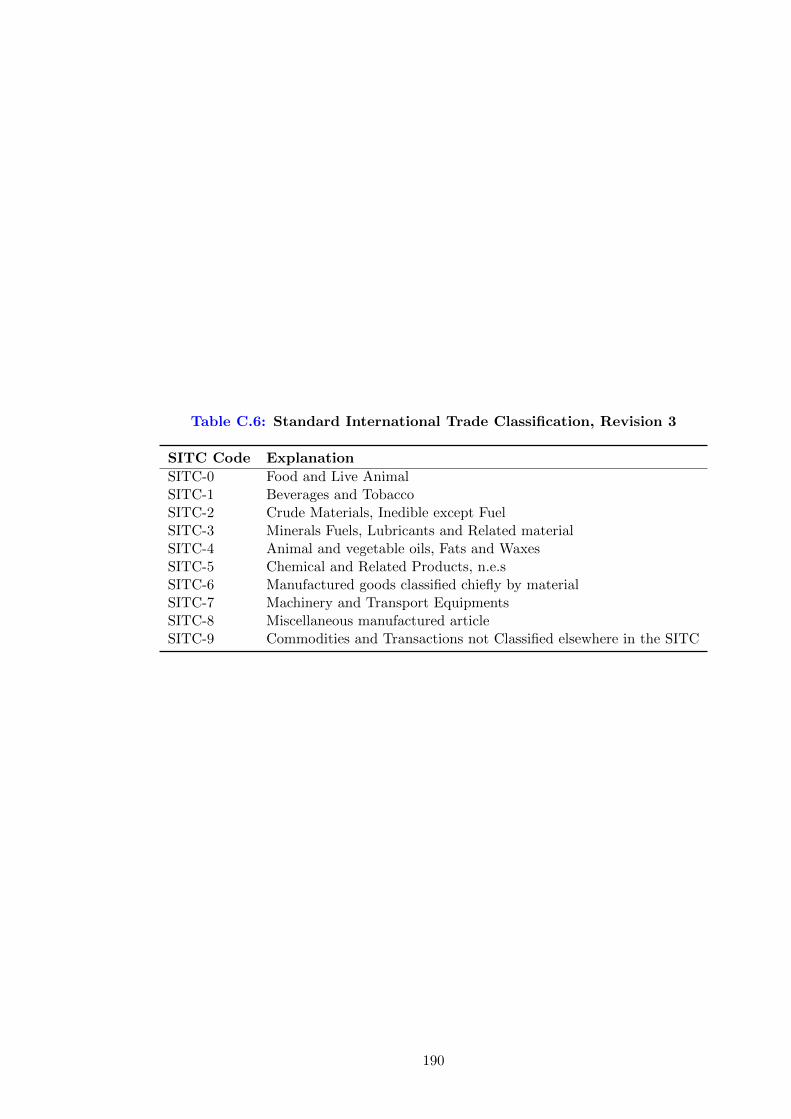
Table C.6: Standard International Trade Classification, Revision 3

SITC Code Explanation

SITC-0 Food and Live AnimalSITC-1 Beverages and TobaccoSITC-2 Crude Materials, Inedible except FuelSITC-3 Minerals Fuels, Lubricants and Related materialSITC-4 Animal and vegetable oils, Fats and WaxesSITC-5 Chemical and Related Products, n.e.sSITC-6 Manufactured goods classified chiefly by materialSITC-7 Machinery and Transport EquipmentsSITC-8 Miscellaneous manufactured articleSITC-9 Commodities and Transactions not Classified elsewhere in the SITC

190

Tab

leC

.7:

Weig

hte

dM

ean

Ap

pli

ed

Tari

ffR

ate

s(%

)in

EU

Mem

ber

Cou

ntr

ies

Country

Name

1988

1989

1990

1991

1992

1993

1994

1995

1996

1997

1998

1999

2000

2001

2002

2003

2004

2005

2006

2007

2008

2009

2010

Austria

3.59

3.77

5.05

4.74

4.46

4.12

4.44

6.27

4.01

3.62

3.29

3.13

2.14

3.02

1.99

2.03

2.07

1.84

1.85

1.81

1.77

1.51

1.61

Belgiu

m3.59

3.77

5.05

4.74

4.46

4.12

4.44

6.27

4.01

3.62

3.29

3.13

2.14

3.02

1.99

2.03

2.07

1.84

1.85

1.81

1.77

1.51

1.61

Bulgaria

3.59

3.77

5.05

4.74

4.46

4.12

4.44

6.27

4.01

3.62

3.29

3.13

2.14

3.02

1.99

2.03

2.07

1.84

1.85

1.81

1.77

1.51

1.61

Cypru

s3.59

3.77

5.05

4.74

4.46

4.12

4.44

6.27

4.01

3.62

3.29

3.13

2.14

3.02

1.99

2.03

2.07

1.84

1.85

1.81

1.77

1.51

1.61

Czech

Republic

3.59

3.77

5.05

4.74

4.46

4.12

4.44

6.27

4.01

3.62

3.29

3.13

2.14

3.02

1.99

2.03

2.07

1.84

1.85

1.81

1.77

1.51

1.61

Denmark

3.59

3.77

5.05

4.74

4.46

4.12

4.44

6.27

4.01

3.62

3.29

3.13

2.14

3.02

1.99

2.03

2.07

1.84

1.85

1.81

1.77

1.51

1.61

Estonia

3.59

3.77

5.05

4.74

4.46

4.12

4.44

6.27

4.01

3.62

3.29

3.13

2.14

3.02

1.99

2.03

2.07

1.84

1.85

1.81

1.77

1.51

1.61

Fin

land

3.59

3.77

5.05

4.74

4.46

4.12

4.44

6.27

4.01

3.62

3.29

3.13

2.14

3.02

1.99

2.03

2.07

1.84

1.85

1.81

1.77

1.51

1.61

Fra

nce

3.59

3.77

5.05

4.74

4.46

4.12

4.44

6.27

4.01

3.62

3.29

3.13

2.14

3.02

1.99

2.03

2.07

1.84

1.85

1.81

1.77

1.51

1.61

Germ

any

3.59

3.77

5.05

4.74

4.46

4.12

4.44

6.27

4.01

3.62

3.29

3.13

2.14

3.02

1.99

2.03

2.07

1.84

1.85

1.81

1.77

1.51

1.61

Gre

ece

3.59

3.77

5.05

4.74

4.46

4.12

4.44

6.27

4.01

3.62

3.29

3.13

2.14

3.02

1.99

2.03

2.07

1.84

1.85

1.81

1.77

1.51

1.61

Hungary

3.59

3.77

5.05

4.74

4.46

4.12

4.44

6.27

4.01

3.62

3.29

3.13

2.14

3.02

1.99

2.03

2.07

1.84

1.85

1.81

1.77

1.51

1.61

Italy

3.59

3.77

5.05

4.74

4.46

4.12

4.44

6.27

4.01

3.62

3.29

3.13

2.14

3.02

1.99

2.03

2.07

1.84

1.85

1.81

1.77

1.51

1.61

Latv

ia3.59

3.77

5.05

4.74

4.46

4.12

4.44

6.27

4.01

3.62

3.29

3.13

2.14

3.02

1.99

2.03

2.07

1.84

1.85

1.81

1.77

1.51

1.61

Lithuania

3.59

3.77

5.05

4.74

4.46

4.12

4.44

6.27

4.01

3.62

3.29

3.13

2.14

3.02

1.99

2.03

2.07

1.84

1.85

1.81

1.77

1.51

1.61

Luxembourg

3.59

3.77

5.05

4.74

4.46

4.12

4.44

6.27

4.01

3.62

3.29

3.13

2.14

3.02

1.99

2.03

2.07

1.84

1.85

1.81

1.77

1.51

1.61

Malta

3.59

3.77

5.05

4.74

4.46

4.12

4.44

6.27

4.01

3.62

3.29

3.13

2.14

3.02

1.99

2.03

2.07

1.84

1.85

1.81

1.77

1.51

1.61

Neth

erlands

3.59

3.77

5.05

4.74

4.46

4.12

4.44

6.27

4.01

3.62

3.29

3.13

2.14

3.02

1.99

2.03

2.07

1.84

1.85

1.81

1.77

1.51

1.61

Poland

3.59

3.77

5.05

4.74

4.46

4.12

4.44

6.27

4.01

3.62

3.29

3.13

2.14

3.02

1.99

2.03

2.07

1.84

1.85

1.81

1.77

1.51

1.61

Portugal

3.59

3.77

5.05

4.74

4.46

4.12

4.44

6.27

4.01

3.62

3.29

3.13

2.14

3.02

1.99

2.03

2.07

1.84

1.85

1.81

1.77

1.51

1.61

Romania

3.59

3.77

5.05

4.74

4.46

4.12

4.44

6.27

4.01

3.62

3.29

3.13

2.14

3.02

1.99

2.03

2.07

1.84

1.85

1.81

1.77

1.51

1.61

Slovakia

3.59

3.77

5.05

4.74

4.46

4.12

4.44

6.27

4.01

3.62

3.29

3.13

2.14

3.02

1.99

2.03

2.07

1.84

1.85

1.81

1.77

1.51

1.61

Slovenia

3.59

3.77

5.05

4.74

4.46

4.12

4.44

6.27

4.01

3.62

3.29

3.13

2.14

3.02

1.99

2.03

2.07

1.84

1.85

1.81

1.77

1.51

1.61

Spain

3.59

3.77

5.05

4.74

4.46

4.12

4.44

6.27

4.01

3.62

3.29

3.13

2.14

3.02

1.99

2.03

2.07

1.84

1.85

1.81

1.77

1.51

1.61

Sweden

3.59

3.77

5.05

4.74

4.46

4.12

4.44

6.27

4.01

3.62

3.29

3.13

2.14

3.02

1.99

2.03

2.07

1.84

1.85

1.81

1.77

1.51

1.61

United

Kin

gdom

3.59

3.77

5.05

4.74

4.46

4.12

4.44

6.27

4.01

3.62

3.29

3.13

2.14

3.02

1.99

2.03

2.07

1.84

1.85

1.81

1.77

1.51

1.61

Fig

ure

sare

taken

from

Worl

dB

ank

web

site

,htt

p:/

/data

.worl

dbank.o

rg/in

dic

ato

r/T

M.T

AX

.MR

CH

.WM

.AR

.ZS.

Wei

ghte

dm

ean

applied

tari

ffis

the

aver

age

of

effec

tivel

yapplied

rate

sw

eighte

dby

the

pro

duct

imp

ort

share

sco

rres

pondin

gto

each

part

ner

countr

y.D

ata

are

class

ified

usi

ng

the

Harm

oniz

edSyst

emof

trade

at

the

six-

or

eight-

dig

itle

vel

.T

ari

ffline

data

wer

em

atc

hed

toSta

ndard

Inte

rnati

onal

Tra

de

Cla

ssifi

cati

on

(SIT

C)

revis

ion

3co

des

todefi

ne

com

modit

ygro

ups

and

imp

ort

wei

ghts

.T

oth

eex

tent

poss

ible

,sp

ecifi

cra

tes

hav

eb

een

conver

ted

toth

eir

ad

valo

rem

equiv

ale

nt

rate

sand

hav

eb

een

incl

uded

inth

eca

lcula

tion

of

wei

ghte

dm

ean

tari

ffs.

Imp

ort

wei

ghts

wer

eca

lcula

ted

usi

ng

the

Unit

edN

ati

ons

Sta

tist

ics

Div

isio

n’s

Com

modit

yT

rade

(Com

trade)

data

base

.E

ffec

tivel

yapplied

tari

ffra

tes

at

the

six-

and

eight-

dig

itpro

duct

level

are

aver

aged

for

pro

duct

sin

each

com

modit

ygro

up.

When

the

effec

tivel

yapplied

rate

isunav

ailable

,th

em

ost

favore

dnati

on

rate

isuse

din

stea

d.

191

Tab

leC

.8:

Intr

aE

UIm

port

s

Year

SIT

CS

ITC

SIT

CS

ITC

SIT

CS

ITC

SIT

CS

ITC

SIT

CS

ITC

01

23

45

67

89

1991

74.8

4312

.186

22.7

4827

.383

3.24

83.8

5712

7.67

827

4.7

56

96.2

54

5.4

619

9282

.635

13.1

3623

.254

25.7

242.

935

91.7

1413

4.42

929

5.5

9104.0

86

6.8

82

1993

69.6

4511

.549

17.9

6520

.538

2.82

877

.775

101.

711

226.7

878.8

12

18.3

74

1994

76.9

9913

.109

22.1

5319

.856

3.60

994

.81

121.

334

263.9

187.6

28

15.5

44

1995

92.9

4215

.41

35.9

3923

.906

4.47

128.

829

189.

981

368.0

16

110.1

83

29.3

48

1996

93.9

6515

.873

32.2

4929

.136

4.92

712

8.24

218

2.23

939

3.8

22

116.3

16

27.9

14

1997

87.4

9515

.823

32.0

2228

.037

4.63

112

7.58

517

9.26

539

6.1

1115.2

01

32.5

78

1998

89.0

9116

.776

31.2

4622

.385

4.62

113

5.82

118

7.98

844

7.8

76

118.6

930.1

79

1999

107.

418

20.8

4635

.591

35.2

515.

305

181.

112

221.

898

534.5

51

141.2

31

36.8

99

2000

96.2

4118

.275

36.7

1556

.208

4.30

218

0.54

215.

2852

1.6

4130.0

32

67.0

75

2001

100.

321

19.6

9634

.909

53.3

884.

616

193.

068

214.

704

533.1

6135.1

08

28.5

420

0211

0.22

822

.136

37.4

5355

.04

5.62

422

6.40

422

6.11

654

9.7

2146.3

76

25.7

04

2003

135.

038

26.1

0744

.16

70.4

466.

905

273.

096

265.

572

637.9

2171.9

72

63.2

78

2004

162.

615

30.9

3261

.296

102.

118.

261

338.

111

355.

3884

1.5

96

221.7

77

86.4

36

2005

174.

636

32.6

3965

.838

143.

847

9.08

237

5.6

376.

707

892.7

66

233.7

57

52.1

35

2006

191.

129

34.2

481

.315

175.

147

10.6

6141

7.54

437.

895

995.2

56

250.9

271.3

820

0722

8.91

440

.573

98.9

7118

1.27

812

.756

490.

685

532.

245

1164.8

299.7

8134.7

11

2008

245.

989

40.3

2996

.195

234.

598

16.9

2749

5.57

152

5.83

911

04.5

79

296.7

12

142.4

85

Fig

ure

sin

billion

dollars

.se

eT

able

C.6

inA

pp

endix

Cfo

rSIT

Cex

pla

nati

on.

192

Tab

leC

.9:

Extr

aE

UIm

port

s

Year

SIT

CS

ITC

SIT

CS

ITC

SIT

CS

ITC

SIT

CS

ITC

SIT

CS

ITC

01

23

45

67

89

1991

54.0

234.

701

42.1

499

.881

2.42

854

.358

104.

913

215.6

5101.6

03

11.6

21

1992

58.9

545.

643

44.5

0299

.389

2.73

861

.014

110.

581

227.9

86

112.4

99

11.8

54

1993

52.6

874.

758

38.3

4985

.212

2.61

758

.118

98.2

35208.7

8109.3

97

11.6

26

1994

59.9

015.

423

48.3

5285

.811

3.51

869

.152

119.

304

238.3

57

118.0

64

11.5

87

1995

66.4

025.

635

50.4

3688

.347

4.16

979

.102

120.

128

256.1

87

124.1

48

14.0

99

1996

68.6

576.

579

46.6

8210

7.62

43.

844

79.7

4811

7.60

527

3.8

72

132.3

82

13.8

92

1997

64.3

956.

915

47.3

9510

4.12

43.

648

81.8

7812

0.15

1293.5

9137.1

115.1

12

1998

65.0

496.

906

46.1

2878

.12

4.12

785

.366

129.

085

328.4

23

144.9

06

14.7

31

1999

54.6

626.

313

41.7

4887

.269

3.34

71.8

9811

3.47

633

1.0

68

147.1

58

7.0

93

2000

52.9

966.

125

47.9

9314

4.67

62.

653

75.7

3612

9.11

936

8.2

38

153.1

718.7

35

2001

55.4

426.

328

45.1

137.

035

2.67

80.7

7112

2.15

434

9.9

18

157.6

06

28.3

93

2002

58.7

176.

747

44.0

0613

9.51

33.

295

88.9

313

0.31

735

4.3

24

166.4

29

21.0

45

2003

70.6

257.

348

51.2

6116

7.47

84.

203

108.

238

154.

706

439.6

68

198.6

91

20.4

12

2004

72.9

867.

7956

.985

219.

311

5.16

912

2.83

116

0.98

245

7.1

86

207.3

223.6

09

2005

79.8

838.

0561

.529

307.

636

5.70

113

6.95

117

9.31

349

4.3

99

229.0

623.5

120

0687

.135

8.27

774

.467

377.

918

7.19

155.

602

223.

513

565.9

75

258.6

38

32.7

45

2007

106.

224

9.60

489

.566

404.

197

8.79

718

7.91

227

7.70

662

5.0

73

291.9

33

29.8

520

0811

1.91

49.

354

91.5

5551

1.83

511

.896

200.

932

270.

291

642.7

08

307.3

78

33.5

66

Fig

ure

sin

billion

dollars

.se

eT

able

C.6

inA

pp

endix

Cfo

rSIT

Cex

pla

nati

on.

193

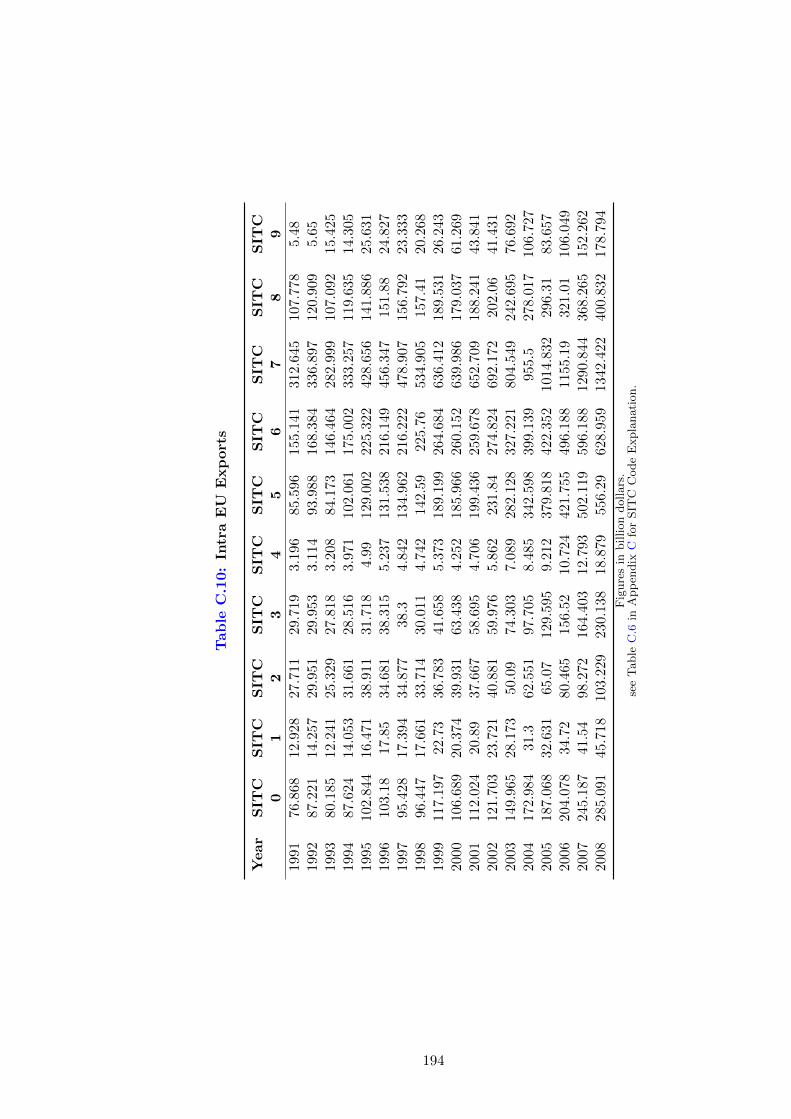
Tab

leC

.10:

Intr

aE

UE

xp

ort

s

Year

SIT

CS

ITC

SIT

CS

ITC

SIT

CS

ITC

SIT

CS

ITC

SIT

CS

ITC

01

23

45

67

89

1991

76.8

6812

.928

27.7

1129

.719

3.19

685

.596

155.

141

312.6

45

107.7

78

5.4

819

9287

.221

14.2

5729

.951

29.9

533.

114

93.9

8816

8.38

433

6.8

97

120.9

09

5.6

519

9380

.185

12.2

4125

.329

27.8

183.

208

84.1

7314

6.46

428

2.9

99

107.0

92

15.4

25

1994

87.6

2414

.053

31.6

6128

.516

3.97

110

2.06

117

5.00

233

3.2

57

119.6

35

14.3

05

1995

102.

844

16.4

7138

.911

31.7

184.

9912

9.00

222

5.32

242

8.6

56

141.8

86

25.6

31

1996

103.

1817

.85

34.6

8138

.315

5.23

713

1.53

821

6.14

945

6.3

47

151.8

824.8

27

1997

95.4

2817

.394

34.8

7738

.34.

842

134.

962

216.

222

478.9

07

156.7

92

23.3

33

1998

96.4

4717

.661

33.7

1430

.011

4.74

214

2.59

225.

7653

4.9

05

157.4

120.2

68

1999

117.

197

22.7

336

.783

41.6

585.

373

189.

199

264.

684

636.4

12

189.5

31

26.2

43

2000

106.

689

20.3

7439

.931

63.4

384.

252

185.

966

260.

152

639.9

86

179.0

37

61.2

69

2001

112.

024

20.8

937

.667

58.6

954.

706

199.

436

259.

678

652.7

09

188.2

41

43.8

41

2002

121.

703

23.7

2140

.881

59.9

765.

862

231.

8427

4.82

469

2.1

72

202.0

641.4

31

2003

149.

965

28.1

7350

.09

74.3

037.

089

282.

128

327.

221

804.5

49

242.6

95

76.6

92

2004

172.

984

31.3

62.5

5197

.705

8.48

534

2.59

839

9.13

995

5.5

278.0

17

106.7

27

2005

187.

068

32.6

3165

.07

129.

595

9.21

237

9.81

842

2.35

210

14.8

32

296.3

183.6

57

2006

204.

078

34.7

280

.465

156.

5210

.724

421.

755

496.

188

1155.1

9321.0

1106.0

49

2007

245.

187

41.5

498

.272

164.

403

12.7

9350

2.11

959

6.18

812

90.8

44

368.2

65

152.2

62

2008

285.

091

45.7

1810

3.22

923

0.13

818

.879

556.

2962

8.95

913

42.4

22

400.8

32

178.7

94

Fig

ure

sin

billion

dollars

.se

eT

able

C.6

inA

pp

endix

Cfo

rSIT

CC

ode

Expla

nati

on.

194

Tab

leC

.11:

EU

Exp

ort

sto

Rest

of

the

Worl

d

Year

SIT

CS

ITC

SIT

CS

ITC

SIT

CS

ITC

SIT

CS

ITC

SIT

CS

ITC

01

23

45

67

89

1991

31.6

2910

.848

11.8

7319

.225

1.70

568

.148

87.4

1923

0.075

70.1

42

15.7

75

1992

37.1

5912

.423

12.7

4918

.987

1.94

476

.372

95.2

1625

0.503

77.2

91

15.6

919

9334

.235

11.7

3911

.951

19.9

821.

761

75.1

6789

.936

238.

201

73.5

28

24.5

75

1994

37.6

8813

.601

13.4

1720

.874

2.24

485

.798

102.

418

273.0

64

82.9

64

25.7

57

1995

44.8

2815

.185

16.3

6122

.042

2.95

910

2.23

812

3.87

833

0.4

64

97.5

62

31.7

53

1996

44.7

9516

.075

15.9

9425

.66

2.72

310

5.18

712

4.85

135

3.903

102.8

729.6

48

1997

44.6

7216

.331

16.2

4823

.275

3.15

310

9.93

812

3.52

836

1.5

93

104.4

58

22.8

42

1998

41.9

5315

.464

14.8

1119

.189

3.33

113.

9111

8.99

371.5

95

104.0

920.8

82

1999

31.4

1113

.342

12.3

0318

.201

2.53

106.

721

104.

946

326.4

09

90.1

89

25.3

27

2000

30.9

5713

.241

13.8

828

.956

2.14

510

8.60

411

1.36

834

6.865

94.4

73

69.4

65

2001

30.9

9513

.427

13.2

0125

.113

1.92

211

6.73

410

6.44

234

6.0

21

97.1

49

85.8

67

2002

33.0

6215

.051

15.0

3627

.045

2.31

113

6.44

118.

026

360.5

58

103.5

879.4

48

2003

38.3

3317

.538

17.8

6934

.588

2.59

316

2.29

213

5.82

942

4.2

21

118.5

65

79.0

17

2004

42.1

2519

.082

22.7

1547

.069

3.08

819

0.65

216

6.24

251

0.0

6138.5

93

82.6

78

2005

44.9

1620

.532

25.6

2362

.268

3.16

220

9.32

318

4.33

956

3.3

18

148.1

185.8

76

2006

49.6

6823

.762

31.6

9380

.486

3.27

223

5.96

520

8.51

263

3.0

2164.9

989.3

23

2007

58.5

6327

.499

37.0

2590

.855

3.57

227

4.13

124

4.59

273

8.4

76

185.5

05

108.7

47

2008

72.3

8929

.45

42.0

3112

4.37

24.

808

301.

526

7.44

182

6.758

202.8

88

139.8

06

Fig

ure

sin

billion

dollars

.se

eT

able

C.6

inA

pp

endix

Cfo

rSIT

Cex

pla

nati

on.

195

Tab

leC

.12:

Som

ech

ara

cte

rist

ics

of

the

Eu

rop

ean

Un

ion

cou

ntr

ies

Exte

nsi

onC

OU

NT

RY

YP

YR

ES

DIS

TK

/LT

ari

f1T

ari

f2T

ari

f3T

ari

f4

Bel

giu

m29

72.2

6028

4.84

714

4.30

159

04.0

4413

38.7

242.

738

2.7

38

2.3

10

Fra

nce

1529

5.48

025

1.58

176

9.22

361

73.0

9610

58.7

413.4

65

4.2

26

3.4

65

2.3

10

Fou

ndin

gG

erm

any

2181

0.03

026

6.13

511

67.5

5561

71.9

1810

82.4

053.3

48

4.2

05

3.3

48

2.3

10

Mem

ber

sIt

aly

1295

2.26

022

5.34

480

6.65

959

02.2

3411

22.6

513.4

81

4.2

27

3.4

81

2.3

10

Lu

xem

bou

rg29

0.29

363

1.12

02.

354

4858

.806

3005

.668

2.7

18

2.7

18

2.3

10

Net

her

lan

ds

4387

.335

277.

736

363.

237

6156

.097

1158

.058

3.4

73

4.2

28

3.4

73

2.3

10

Den

mar

k13

662.

040

2569

.814

234.

022

5960

.626

9324

.386

3.439

4.2

09

3.4

39

2.3

10

1st

Irel

and

1099

.932

280.

205

61.8

9960

11.8

0513

73.7

233.

443

4.2

38

3.4

43

2.3

10

Un

ited

Kin

gdom

1008

3.81

017

0.91

051

0.13

864

27.2

2458

5.88

23.4

87

4.2

28

3.4

87

2.3

10

2nd

Gre

ece

1586

.142

146.

513

134.

759

5120

.412

715.

890

3.437

4.2

25

3.4

37

2.3

10

3rd

Por

tuga

l13

43.4

5613

0.72

522

2.81

858

26.6

4063

5.54

63.

413

4.2

30

3.4

13

2.3

10

Sp

ain

7105

.264

173.

426

562.

199

5886

.856

983.

490

3.5

03

4.2

36

3.5

03

2.3

30

Au

stri

a22

35.8

9727

8.28

520

3.81

954

21.3

4413

26.9

153.3

84

4.2

26

3.3

84

2.3

10

4th

Fin

lan

d13

28.7

3825

7.30

598

.478

5647

.318

1024

.297

3.437

4.2

34

3.4

37

2.3

10

Sw

eden

2328

4.26

026

22.4

7623

0.07

659

96.4

1490

50.7

203.4

52

4.2

30

3.4

52

2.3

10

Cyp

rus

111.

258

117.

650

29.6

0241

72.7

2747

9.30

83.

392

4.4

13

3.3

92

2.3

10

Cze

chR

ep.

4961

.782

Est

onia

1457

.574

1073

.310

16.9

1346

77.0

7166

03.4

883.0

01

3.0

01

2.3

10

5th

Hu

nga

ry18

5980

.500

1826

8.25

019

5.04

647

57.8

4498

691.

300

3.243

4.0

38

3.2

43

2.3

11

Lat

via

78.1

1733

.609

23.2

5342

81.6

2218

3.06

33.0

04

4.3

50

3.0

04

2.3

10

Lit

hu

ania

613.

984

177.

681

31.5

3941

89.5

7185

9.89

03.0

63

4.2

25

3.0

63

2.3

09

Mal

ta42

.979

110.

486

22.1

7943

47.7

0958

9.56

83.

321

4.5

75

3.3

21

2.3

09

Pol

and

8968

.603

234.

178

381.

387

4871

.189

1034

.336

3.0

99

4.0

14

3.0

99

2.3

10

Slo

vakia

461.

052

85.6

1010

6.45

543

95.9

7848

2.82

23.

125

4.3

50

3.1

25

2.3

11

Slo

ven

ia25

2.50

712

6.35

350

.471

4409

.432

656.

387

3.1

60

3.8

48

3.1

60

2.3

30

6th

Bu

lgar

ia41

0.71

952

.146

88.3

7847

34.0

7224

9.89

02.8

66

2.8

66

2.3

09

Rom

ania

2464

.418

111.

769

2290

.297

4537

.797

508.

098

3.3

27

4.3

33

3.3

27

2.3

10

Y=

Rea

lG

DP

inB

illion,

PY

=P

erC

apit

aR

eal

GD

P,R

ES=

Fore

ign

Res

erves

inB

illion,

K/L

=C

apit

al

Lab

or

rati

o

Tari

f1=

Aver

age

tari

fffo

r1988-2

008,

Tari

f2=

Aver

age

tari

fffo

r1988-1

994,T

ari

f3=

Aver

age

tari

fffo

r1995-2

003,

Tari

f4=

Aver

age

tari

fffo

r2004-2

008

Y,

PY

,D

IST

,R

ES

Valu

esare

the

aver

ages

for

each

countr

yfo

r1998-2

008

196

Table C.13: Summary Statistics

Variable Obs Mean Std. Min Max

Yj 480496 425054.5 2377581 0.018 37800000Yi 564322 12954.03 31730.91 28.2841 227918.2Rj 472632 612000000 29400000000 0.0007 1.95E+12Ri 564322 413.0327 1361.989 1.0921 43515.38eij 294619 1020000000 1.42E+11 9.42E-10 2.41E+13SIM 464623 -1.75128 1.318097 -15.85478 -0.6931472RF 337910 1.932992 1.676233 0.0001331 11.80068dij 557095 5555.734 3913.962 59.61723 19586.18

Values are the average of all the countries included in the sample

Values of Yj , Yi, Rj and Ri are in billions and others are in units

197

Table C.14: Trading Partners of the EU

Afghanistan, Albania, Algeria, American Samoa, Andorra, Angola, Antarctica, Antigua andBarbuda, Argentina, Armenia, Aruba, Australia, Austria, Azerbaijan, Bahamas, Bahrain,Bangladesh, Barbados, Belarus, Belgium, Belize, Benin, Bermuda, Bhutan, Bolivia, Bosniaand Herzegovina, Botswana, Bouvet Island, Brazil, Brunei Darussalam, Bulgaria, Bunkers,Burkina Faso, Burundi, Cambodia,Cameroon, Canada, Cape Verde, Cayman Island, Chad, Chile,China, Christmas Island, Cocos Island, Colombia, Comoros, Congo Democratic Republic, CongoRepublic, Cook Island, Costa Rica, Cote d’Ivoire, Croatia, Cuba, Cyprus, Czech Republic,Czechoslovakia, Denmark, Djibouti, Dominica, Dominican Republic, Ecuador, Egypt, ArabRepublic, El Salvador, Equatorial Guinea, Eritrea, Estonia, Ethiopia, Faeroe Islands, FalklandIsland, Fiji, Finland, Fmr Arab Republic of Yemen, Fmr Democratic Republic of Germany,Fmr Democratic Yemen, Fmr Ethiopia, Fmr Fed. Republic of Germany, Fmr USSR, FmrYugoslavia, France, French Guiana, French Polynesia, Gabon, Gambia, Georgia, Germany, Ghana,Gibraltar, Greece, Greenland, Grenada, Guadeloupe, Guam, Guatemala, Guinea, Guinea-Bissau,Guyana, Haiti, Heard Island and McDonald Islands, Holy See (Vatican City State), Honduras,Hong Kong SAR China, Hungary, Iceland, India, Indonesia, Iran, Iraq, Ireland, Israel, Italy,Jamaica, Japan, Jordan, Kazakhstan, Kenya, Kiribati, Korea Democratic Republic, KoreaRepublic, Kuwait, Kyrgyz Republic, Lao PDR, Latvia, Lebanon, Lesotho, Liberia, Libya,Lithuania, Luxembourg, Macao SAR China, Macedonia, FYR, Madagascar, Malawi,Malaysia,Maldives, Mali, Malta, Marshall Islands, Martinique, Mauritania, Mauritius, Mayotte, Mexico,Micronesia, Moldova, Mongolia, Montenegro, Montserrat, Morocco, Mozambique, Myanmar,Namibia, Nauru, Nepal, Netherlands, New Caledonia, New Zealand, Nicaragua, Niger, Nigeria,Niue, Norfolk Island, Northern Mariana Islands, Norway, Oman, Pakistan, Palau, Panama, PapuaNew Guinea, Paraguay, Peru, Philippines, Pitcairn, Poland, Portugal, Qatar, Romania, RussianFederation, Rwanda, Saint Helena, Saint Pierre and Miquelon, Samoa, San Marino, Sao Tomeand Principe, Saudi Arabia, Senegal, Serbia, Seychelles, Sierra Leone, Singapore, Slovak Republic,Slovenia, Solomon Islands, Somalia, South Africa, South Georgia and the South Sandwich Island,Spain, Sri Lanka, Saint Kitts and Nevis, Saint Lucia, Saint Vincent and the Grenadines, Sudan,Suriname, Swaziland, Sweden, Switzerland, Syrian Arab Republic, Tajikistan, Tanzania, Thailand,Timor-Leste, Togo, Tokelau, Tonga, Trinidad and Tobago, Tunisia, Turkey, Turkmenistan, Turksand Caicos Islands, Tuvalu, Uganda, Ukraine, United Arab Emirates, United Kingdom, UnitedStates, Uruguay, Uzbekistan, Vanuatu, Venezuela, RB, Vietnam, Virgin Islands (U.S.),Wallis and Futuna Island, West Bank and Gaza, Yemen, Republic, Zambia, Zimbabwe

198

Figure 21: Levels of Economic Integration

Free Trade

among Members Common

External Tariff Free Factor Movements

Macro Policy Harmonization

Free Trade Area

Custom Union

Common Market

Economic Union

A Free Trade Area is an agreement in which two or more than two countries agree to remove all the tariff and non-tariff barriers and the quantitative restrictions on their mutual trade. However, each member of the group is free to adopt and maintain any tariff or regulations on the trade with non-member country. A Custom Union is an agreement in which two or more than two countries agree to remove all the tariff and non-tariff barriers and the quantitative restrictions on their mutual trade, plus a common external tariff on the trade with non-member countries. A Common Market is an agreement in which two or more than two countries agree to remove all the tariff and non-tariff barriers and the quantitative restrictions on their mutual trade, adopt of a common external tariff on the trade with non-member countries, plus a free movement of the factors of production among the member countries. An Economic Union is an agreement in which two or more than two countries agree to remove all the tariff and non-tariff barriers and the quantitative restrictions on their mutual trade, adopt a common external tariff on the trade with non-member countries, a free movement of the factors of productions, and harmonization of the macro economic policies.

199

References

Abowd, J., P. Corbel, and F. Kramarz (1999). The entry and exit of workers and thegrowth of employment: an analysis of French establishments. Review of Economics andStatistics 81 (2), 170–187.

Amiti, M. and D. Weinstein (2011). Exports and financial shocks. The Quarterly Journalof Economics 126 (4), 1841–1877.

Anderson, J. (1979). A theoretical foundation for the gravity equation. The AmericanEconomic Review 69 (1), 106–116.

Anderson, J. and E. Van Wincoop (2004). Trade costs. Journal of Economic Litera-ture 42 (3), 691–751.

Arellano, M. and O. Bover (1995). Another look at the instrumental variable estimationof error-components models. Journal of econometrics 68 (1), 29–51.

Auboin, M. (2009). Boosting the availability of trade finance in the current crisis: back-ground analysis for a substantial G20 package. CEPR Policy Insight 35.

Auer, R. and T. Chaney (2009). Exchange Rate Pass-Through in a Competitive Model ofPricing-to-Market. Journal of Money, Credit and Banking 41 (s1), 151–175.

Baier, S. and J. Bergstrand (2007). Do free trade agreements actually increase members’international trade? Journal of International Economics 71 (1), 72–95.

Baier, S. L. and J. H. Bergstrand (2004). Economic determinants of free trade agreements.Journal of International Economics 64 (1), 29–63.

Balassa, B. (1967). Trade creation and trade diversion in the European Common Market.The Economic Journal 77 (305), 1–21.

Balassa, B. (1986). The determinants of intra-industry specialization in united statestrade. Oxford Economic Papers 38 (2), 220–233.

Balassa, B. and L. Bauwens (1987). Intra-industry specialisation in a multi-country andmulti-industry framework. The Economic Journal 97 (388), 923–939.

Baldwin, R. (2009). The great trade collapse: Causes, Consequences and Prospects. Cepr.

Baldwin, R. E. (1994). Towards an integrated Europe, Volume 25. Citeseer.

Baldwin, R. E. and A. J. Venables (1995). Regional economic integration. Handbook ofinternational economics 3, 1597–1644.

Baldwin, R. E. and C. Wyplosz (2009). The economics of European integration, Volume 3.McGraw-Hill London.

Bayoumi, T. and B. Eichengreen (1997). Is regionalism simply a diversion? evidence fromthe evolution of the ec and efta. In Regionalism versus Multilateral Trade Arrangements,NBER-EASE Volume 6, pp. 141–168. University of Chicago Press.

Beck, T. (2002). Financial dependence and international trade: is there a link? Journalof International Economics 57 (1), 107–131.

Beck, T. (2003). Financial dependence and international trade. Review of InternationalEconomics 11 (2), 296–316.

BEEPS (2010). BEEPS At-A-Galance 2008 Cross Country Report. Business Environmentand Enterprise Performance Surveys(BEEPS), The World Bank Group, 1–60.

Bergstrand, J. (1985). The gravity equation in international trade: some microeconomicfoundations and empirical evidence. The review of economics and statistics 67 (3), 474–481.

Bergstrand, J. (1989). The generalized gravity equation, monopolistic competition, andthe factor-proportions theory in international trade. The Review of Economics andStatistics 71 (1), 143–153.

200

Berman, N. and J. Hericourt (2010). Financial factors and the margins of trade: Evidencefrom cross-country firm-level data. Journal of Development Economics 93 (2), 206–217.

Bhagwati, J. (1971). Trade-diverting customs unions and welfare-improvement: A clarifi-cation. The Economic Journal 81 (323), 580–587.

Blundell, R. and S. Bond (1998). Initial conditions and moment restrictions in dynamicpanel data models. Journal of econometrics 87 (1), 115–143.

BOE (2011). Financial Stability Report, 2011, Issue No. 30. Bank of England (BOE).

Bordo, M. (2008). The crisis of 2007: some lessons from history.The First Global Financial Crisis of the 21st Century, available athttp://cid.bcrp.gob.pe/biblio/Papers/Documentos/The%20first%20global%20financial%20crisis%20of%20the%2021st%20century.pdf#page=61 ,51.

Brancaccio, E. and G. Fontana (2010). The conventional views of the global crisis: A criti-cal assessment. An Assessment of the Global Impact of the Financial Crisis. Houndmills(Basingstoke, UK): Palgrave Macmillan..

Braun, M. (2003). Financial contractibility and asset hardness. University of California-Los Angeles mimeo.

Brennan, M., V. Miksimovic, and J. Zechner (1988). Vendor financing. The Journal ofFinance 43 (5), 1127–1141.

Bricongne, J., L. Fontagne, G. Gaulier, D. Taglioni, and V. Vicard (2012). Firms and theglobal crisis: French exports in the turmoil. Journal of International Economics 87 (1),134–146.

Bridges, S. and A. Guariglia (2008). Financial constraints, global engagement, and firmsurvival in the united kingdom: evidence from micro data. Scottish Journal of PoliticalEconomy 55 (4), 444–464.

Brunnermeier, M. (2009). Deciphering the liquidity and credit crunch 2007-08. Journalof Economic Perspectives 23 (1), 77–100.

Buch, C., I. Kesternich, A. Lipponer, and M. Schnitzer (2009). Financial Constraints andthe Margins of FDI. Centre for Economic Policy Research (7444).

Buiter, W. H. (2000). Optimal currency areas scottish economic society/royal bank ofscotland annual lecture, 1999. Scottish Journal of Political Economy 47 (3), 213–250.

Burgess, S. and M. Knetter (1998). An international comparison of employment adjust-ment to exchange rate fluctuations. Review of International Economics 6 (1), 151–163.

Campa, J. and L. Goldberg (2001). Employment versus wage adjustment and the USdollar. Review of Economics and Statistics 83 (3), 477–489.

Campa, J. and M. J. Gonzalez (2006). Differences in exchange rate pass-through in theeuro area. European Economic Review 50 (1), 121–145.

Carrere, C. (2006). Revisiting the effects of regional trade agreements on trade flows withproper specification of the gravity model. European Economic Review 50 (2), 223–247.

Chauffour, J. and M. Malouche (2011). Trade finance during the 2008–9 trade collapse:Key takeaways. World Bank-Economic Premise (66), 1–6.

Chit, M., M. Rizov, and D. Willenbockel (2010). Exchange rate volatility and exports:New empirical evidence from the emerging East Asian Economies. The World Econ-omy 33 (2), 239–263.

Chor, D. and K. Manova (2011). Off the cliff and back? credit conditions and internationaltrade during the global financial crisis. Journal of International Economics.

Claessens, S. and L. Laeven (2003). Financial development, property rights, and growth.The Journal of Finance 58 (6), 2401–2436.

201

Clarete, R., C. Edmonds, and J. Wallack (2003). Asian regionalism and its effects on tradein the 1980s and 1990s. Journal of Asian Economics 14 (1), 91–129.

Clausing, K. (2001). Trade creation and trade diversion in the Canada–UnitedStates free trade agreement. Canadian Journal of Economics/Revue canadienned’economique 34 (3), 677–696.

Cobham, D. (2002). The exchange rate as a source of disturbances: The uk 1979-2000.National Institute Economic Review 181 (1), 96–112.

Cobham, D. (2006). The overvaluation of sterling since 1996: How the policy makersresponded and why. The Economic Journal 116 (512), F185–F207.

Cooper, H. W. (2006). Free Trade Agreements: Impact on U.S. Trade andImplications for U.S. Trade Policy. CRS Report for Congress, available athttphttp://fpc.state.gov/documents/organization/70293.pdf .

COP (2009). April Oversight Report. Congressional Oversight Panel (COP), Washington,DC .

Corsetti, G., L. Dedola, and S. Leduc (2008). High exchange-rate volatility and low pass-through. Journal of Monetary Economics 55 (6), 1113–1128.

Cuyvers, L. (1997). Trade diversion effects of the new EU arrangements on ASEAN. AsianEconomic Journal 11 (3), 243–263.

Das, D. (2010). Current global financial crisis: The great recession and nascent recovery.Globalization Development Centre, Bond University Working Paper (35).

Das, S., M. Roberts, and J. Tybout (2007). Market entry costs, producer heterogeneity,and export dynamics. Econometrica 75 (3), 837–873.

Datta, A. and M. Kouliavtsev (2009). NAFTA and the Realignment of Textile and ApparelTrade: Trade Creation or Trade Diversion? Review of International Economics 17 (1),172–186.

Davis, S., J. Haltiwanger, and S. Schuh (1996). Job creation and job destruction. Cam-bridge, MA: MIT Press.

De Larosiere, J. (2009). The High-Level Group on financial supervision in the EU: report.European Commission.

Deardorff, A. (1998). Determinants of bilateral trade: does gravity work in a neoclassicalworld? Regionalization of the World Economy, edited by Frankel, J., University ofChicago Press.

Draca, M., S. Machin, and J. Van Reenen (2008). Minimum wages and firm profitability.Technical report, National Bureau of Economic Research.

Edmonds, T., T. Jarrett, and J. Woodhouse (2010). The credit crisis: A timeline. Houseof Commons Library, Standard Notes, No. SN/BT/4991.

Egger, P. (2000). A note on the proper econometric specification of the gravity equation.Economics Letters 66 (1), 25–31.

Egger, P. and M. Pfaffermayr (2003). The proper panel econometric specification of thegravity equation: A three-way model with bilateral interaction effects. Empirical Eco-nomics 28 (3), 571–580.

Engel, C. (1999). Accounting for US Real Exchange Rate Changes. Journal of PoliticalEconomy 107 (3), 507–538.

EUCOM (2009). The General Report on the Activities of the EuropeanUnion 2009. European Commission (EUCOM) report 2009, available at,http://europa.eu/generalreport/en/2009/files/rg2009 en.pdf .

Evenett, S. and W. Keller (2002). On theories explaining the success of the gravityequation. Journal of Political Economy 110 (2), 281–316.

202

Faggio, G., K. G. Salvanes, and J. Van Reenen (2010). The evolution of inequality inproductivity and wages: panel data evidence. Industrial and Corporate Change 19 (6),1919–1951.

Fisman, R. and I. Love (2003). Trade credit, financial intermediary development, andindustry growth. The Journal of Finance 58 (1), 353–374.

Frankel, J. and A. Rose (2002). An estimate of the effect of common currencies on tradeand income. The Quarterly Journal of Economics 117 (2), 437–466.

Frankel, J. A. (1997). Regional trading blocs in the world trading system. Institute forInternational Economics, Washington DC .

Garcia-Vega, M., A. Guariglia, and M. Spaliara (2012). Volatility, financial constraints,and trade. International Review of Economics & Finance 21 (1), 57–76.

Gehrels, F. (1956). Customs union from a single-country viewpoint. The Review of Eco-nomic Studies 24 (1), 61–64.

Georges, P. (2008). Liberalizing NAFTA Rules of Origin: A Dynamic CGE Analysis.Review of International Economics 16 (4), 672–691.

Girma, S., H. Gorg, and A. Hanley (2008). R&d and exporting: A comparison of britishand irish firms. Review of World Economics 144 (4), 750–773.

Gomez-Salvador, R., J. Messina, and G. Vallanti (2004). Gross job flows and institutionsin Europe. Labour Economics 11 (4), 469–485.

Goto, J. and K. Hamada (1999). Regional economic integration and Article XXIV of theGATT. Review of International Economics 7 (4), 555–570.

Gourinchas, P. O. (1999). High Exchnage Rates Do Matter: French Job Reallocation andExchange Rate Turbulence. European Economic Review 43 (7), 1279–1316.

Greenaway, D., A. Guariglia, and R. Kneller (2007). Financial factors and exportingdecisions. Journal of International Economics 73 (2), 377–395.

Greenaway, D., R. Hine, and P. Wright (1999). An empirical assessment of the impactof trade on employment in the United Kingdom. European Journal of Political Econ-omy 15 (3), 485–500.

Greenhalgh, C. and M. Rogers (2006). The value of innovation: The interaction of com-petition, r&d and ip. Research Policy 35 (4), 562–580.

Guariglia, A. and S. Mateut (2010). Inventory investment, global engagement, and finan-cial constraints in the UK: evidence from micro data. Journal of Macroeconomics 32 (1),239–250.

Gust, C., S. Leduc, and R. Vigfusson (2010). Trade integration, competition, and thedecline in exchange-rate pass-through. Journal of Monetary Economics 57 (3), 309–324.

Harris, R. and Q. Li (2007). Firm level empirical study of the contribution of exportingto uk productivity growth. Report submitted to UKTI March.

Helpman, E. (1987). Imperfect competition and international trade: Evidence from four-teen industrial countries. Journal of the Japanese and international economies 1 (1),62–81.

Hijzen, A., M. Pisu, R. Upward, and P. Wright (2011). Employment, job turnover,and trade in producer services: Uk firm-level evidence. Canadian Journal of Eco-nomics/Revue canadienne d’economique 44 (3), 1020–1043.

Hijzen, A., R. Upward, and P. Wright (2010). Job Creation, Job Destruction and the Roleof Small Firms: Firm-Level Evidence for the UK. Oxford Bulletin of Economics andStatistics 72 (5), 621–647.

Hur, J., M. Raj, and Y. Riyanto (2006). Finance and trade: A cross-country empiricalanalysis on the impact of financial development and asset tangibility on internationaltrade. World Development 34 (10), 1728–1741.

203

Iacovone, L. and V. Zavacka (2009). Banking crises and exports: lessons from the past.World Bank Policy Research Working Paper, No. 5016 .

Jacks, D., C. Meissner, and D. Novy (2009). 18. The role of trade costs in the great tradecollapse. The Great Trade Collapse: Causes, Consequences and Prospects, 159.

Jansen, M. and E. von Uexkuell (2010). Trade and employment in the global crisis. Inter-national Labour Organisation, Geneva, Switzerland.

Kandogan, Y. (2005). Trade creation and diversion effects of europe’s regional liberaliza-tion agreements.

Keuschnigg, C., W. Kohler, A. Casella, and A. Sapir (1996). Austria in the EuropeanUnion: dynamic gains from integration and distributional implications. Economic Pol-icy 11 (22), 155–211.

Klein, M., S. Schuh, and R. Triest (2003). Job creation, job destruction, and the realexchange rate. Journal of International Economics 59 (2), 239–265.

Kletzer, K. and P. Bardhan (1987). Credit markets and patterns of international trade.Journal of Development Economics 27 (1-2), 57–70.

Knetter, M. (1989). Price Discrimination by U.S. and German Exporters. The AmericanEconomic Review 79 (1), 198–210.

Knetter, M. and P. Goldberg (1997). Goods prices and exchange rates: What have welearned? Journal of Economic Literature 35 (3), 1243–1272.

Kono, D. (2002). Are Free Trade Areas Good for Multilateralism? Evidence from theEuropean Free Trade Association. International Studies Quarterly 46 (4), 507–527.

Kowalczyk, C. (2000). Welfare and integration. International Economic Review 41 (2),483–494.

Krugman, P. (1987). The Narrow Moving Band, the Dutch Disease, and the CompetitiveConsequences of Mrs. Thatcher: Notes on Trade in the Presence of Dynamic ScaleEconomies. Journal of Development Economics 27 (1-2), 41–55.

Lambert, D. and S. McKoy (2009). Trade creation and diversion effects of preferential tradeassociations on agricultural and food trade. Journal of Agricultural Economics 60 (1),17–39.

Lee, H., C. Koo, and E. Park (2008). Are Exports of China, Japan and Korea Divertedin the Major Regional Trading Blocs? The World Economy 31 (7), 841–860.

Levchenko, A., L. Lewis, and L. Tesar (2010). The collapse of international trade duringthe 2008-2009 crisis: In search of the smoking gun. IMF Economic Review 58 (2),214–253.

Levchenko, A., L. Lewis, and L. Tesar (2011). The Role of Trade Finance in the US TradeCollapse: A Skeptics View. Trade Finance During the Great Trade Collapse, WorldBank .

Lindsey, B. (2004). Job losses and trade. Cato institute trade briefing paper 19, 1–12.

Lipsey, R. (1957). The theory of customs unions: trade diversion and welfare. Econom-ica 24 (93), 40–46.

Liu, X., P. Siler, C. Wang, and Y. Wei (2000). Productivity spillovers from foreign di-rect investment: evidence from uk industry level panel data. Journal of InternationalBusiness Studies 31 (3), 407–425.

Long, M., I. Malitz, and S. Ravid (1993). Trade credit, quality guarantees, and productmarketability. Financial Management , 117–127.

Makwana, R. (2006). Reforming International Trade. Available at,http://www.stwr.org/imf-world-bank-trade/reforming-international-trade.html .

204

Manova, K., S. Wei, and Z. Zhang (2011). Firm exports and multinational activity undercredit constraints. National Bureau of Economic Research, Working Paper No. 16905 .

Matyas, L. (1997). Proper econometric specification of the gravity model. The worldeconomy 20 (3), 363–368.

Minetti, R. and S. Zhu (2011). Credit constraints and firm export: microeconomic evidencefrom Italy. Journal of International Economics.

Mora, J. and W. Powers (2009). Decline and gradual recovery of global trade financing:US and global perspectives. VoxEU (27 November).

Mordechai, E. K. (1969). Trade Creation and Trade Diversion by the EEC and EFTA.Economia Internationale 22 (s), 273–280.

Moser, C., D. Urban, and B. Di Mauro (2010). International competitiveness, job creationand job destruction–An establishment-level study of German job flows. Journal ofInternational Economics 80 (2), 302–317.

Nguyen, T. and M. Ezaki (2005). Regional economic integration and its impacts on growth,poverty and income distribution: The case of Vietnam. Review of Urban & RegionalDevelopment Studies 17 (3), 197–215.

Oxlade, A. (2012). Economy watch: Is the British economy already back into recession?available at, http://9dj1o x.0.u.is/money/news/article-1616085/Economy-watch-What-Britain.html .

Panagariya, A. (1994). East Asia and the new regionalism in world trade. The WorldEconomy 17 (6), 817–839.

Pelzman, J. (1977). Trade Creation and Trade Diversion in the Council of Mutual Eco-nomic Assistance: 1954-1970. American Economic Review 67 (4), 713–722.

Petersen, M. and R. Rajan (1997). Trade credit: theories and evidence. Review of Finan-cial Studies 10 (3), 661–691.

Polak, J. J. (1996). Is apec a natural regional trading bloc? a critique of the ?gravitymodel?of international trade. The World Economy 19 (5), 533–543.

Poyhonen, P. (1963). Trade Creation and Trade Diversion by the EEC and EFTA.Weltwirtschaftliches Archive 90, 93–100.

Presbitero, A. (2008). The debt-growth nexus in poor countries: a reassessment. Eco-nomics: The Open-Access, Open-Assessment E-Journal 2.

Radelet, S. (1997). Regional Integration and Cooperation in Sub-Saharan Africa: Areformal trade agreements the right strategy? Development Discussion Paper, HarvardInstitutte for Development International Development .

Rajan, R. and L. Zingales (1998). Financial dependence and growth. The AmericanEconomic Review 88 (3), 559–586.

Revenga, A. (1992). Exporting jobs? The Quarterly Journal of Economics 107 (1), 255–284.

Riezman, R. (1979). A 3×3 model of customs unions. Journal of International Eco-nomics 9 (3), 341–354.

Sarker, R. and S. Jayasinghe (2007). Regional trade agreements and trade in agri-foodproducts: evidence for the European Union from gravity modeling using disaggregateddata. Agricultural Economics 37 (1), 93–104.

Sayan, S. (1998). Could Regional Economic Cooperation Generate Trade Creation andTrade Diversion Effects without Altering Trade Policies of Members?: Preliminary Re-sults from a Gravity Application to BSEC. Bilkent Univ., Department of Economics.

Soloaga, I. and W. L. Alan (2001). Regionalism in the nineties: What effect on trade?The North American Journal of Economics and Finance 12 (1), 1–29.

205

Solomon, M. E. (2010). A comparison of spillovers from british and foreign multinationalsin the uk economy. University of Essex, available at, https://editorialexpress.com/cgi-bin/conference/download.cgi?db name=res2011&paper id=142 .

Sura, W. (2009). Industry, Trade and Services. Eurostat: Statistics in focus 62/2009,European Commission. 62.

Thursby, J. G. and M. C. Thursby (1987). Bilateral trade flows, the linder hypothesis,and exchange risk. The Review of Economics and Statistics, 488–495.

Tinbergen, J. (1962). Shaping the world economy: Suggestions for an international eco-nomic policy. Twentieth Century Fund New York.

Turner, A. (2009). A regulatory response to the global banking crisis. The Turner Review .

Viner, J. (1950). The Custom Union Issue. Carnegie Endowment for International PeaceNew York.

Vollrath, T., M. Gehlhar, and C. Hallahan (2009). Bilateral Import Protection, Free TradeAgreements, and Other Factors Influencing Trade Flows in Agriculture and Clothing.Journal of Agricultural Economics 60 (2), 298–317.

Wacziarg, R. (1999). Measuring the Dynamic Gains from Trade. Research Workingpapers 1 (1), 1–50.

Wang, Z. K. and L. A. Winters (1992). The trading potential of eastern europe. Journalof Economic Integration 7 (2), 113–136.

Watcher, L. (2005). The Effects of the FTA on Social Welfare and Urban Employment.International Society for Intercommunication of New Ideas (ISINI) 8th InternationalConference, Wageningen, The Netherlands, August 2005 .

WEO (2010). Do financial crises have lasting effects on trade? IMF, World EcnomicOutlook, October 2010 .

WESS (2010). Retooling the Global Trade. World Economic and Social Survey (WESS)Report, Chapter 4, Economic and Social Affairs Department, United Nation, New York .

Wisniewski, T. and B. Lambe (2011). The role of media in the credit crunch: The case ofthe banking sector. Journal of Economic Behavior & Organization.

WorldBank (2011). World Development Indicators (Edition: September 2011). ESDSInternational, University of Manchester. DOI: http://dx.doi.org/10.5257/wb/wdi/2011-09 .

Wren-Lewis, S. and G. Britain (2003). Estimates of equilibrium exchange rates for sterlingagainst the euro. HM Treasury London.

WTO (2010). Trade to expand by 9.5 percent in 2010 after a dismal 2009. World TradeOrganization Reports, Press Release 598, March 26..

WTO (2011). World Trade Report 2011. World Trade Organization (WTO).

Zahniser, S., D. Pick, G. Pompelli, and M. Gehlhar (2002). Regionalism in the west-ern hemisphere and its impact on US agricultural exports: A gravity-model analysis.American Journal of Agricultural Economics 84 (3), 791–797.

206

The E ects of Real Exchange Rate, External Finance and …etheses.whiterose.ac.uk/4722/1/PhD_Thesis...

Documents

Transcript of The E ects of Real Exchange Rate, External Finance and …etheses.whiterose.ac.uk/4722/1/PhD_Thesis...