The Effects of Globalization on Macroeconomic

Dynamics in a Trade-Dependent Economy:

the Case of Korea

Fabio Milani†

Sung Ho Park‡

The views expressed herein are those of authors and do not nec-

essarily reflect the officical views of the Bank of Korea. When

reporting or citing this paper, the authors’ name should always

be explicitly stated.

†Department of Economics, University of California, Irvine, 3151, Social Science Plaza, Irvine, CA 92697-5100,

U.S.A., E-mail: fmilani@uci.edu

‡Economic Research Institute, Bank of Korea, 39 Namdaemunno, Jung-Gu, Seoul, Korea, E-mail:

pshlhk@bok.or.kr

We would like to thank seminar participants at the Bank of Korea for comments and dis-

cussions. Professor Milani acknowledges and is grateful for the financial support provided

by the Bank of Korea regarding this research project. All remaining errors are our own.

Contents

1 Introduction 1

2 Small Open Economy Model 4

2.1 Model Description . . . . . . . . . . . . . . . . . . . . . . . . . . . . . . . 5

2.1.1 Households . . . . . . . . . . . . . . . . . . . . . . . . . . . . . . . 5

2.1.2 Firms . . . . . . . . . . . . . . . . . . . . . . . . . . . . . . . . . . 7

2.1.3 Exchange Rate, Terms of Trade, Monetary Policy . . . . . . . . . . 8

2.2 Model Summary . . . . . . . . . . . . . . . . . . . . . . . . . . . . . . . . 9

2.3 Non-Fully Rational Expectations . . . . . . . . . . . . . . . . . . . . . . . 11

3 Estimation Details 12

3.1 State Space . . . . . . . . . . . . . . . . . . . . . . . . . . . . . . . . . . . 12

3.2 Data . . . . . . . . . . . . . . . . . . . . . . . . . . . . . . . . . . . . . . . 12

3.3 Bayesian Approach . . . . . . . . . . . . . . . . . . . . . . . . . . . . . . . 16

4 Results 18

4.1 Structural Estimates . . . . . . . . . . . . . . . . . . . . . . . . . . . . . . 18

4.2 Globalization and Macroeconomic Dynamics . . . . . . . . . . . . . . . . . 18

4.3 The Role of Domestic and Global Shocks . . . . . . . . . . . . . . . . . . . 21

5 Robustness 23

6 Conclusions 27

The Effects of Globalization on Macroeconomic Dynamicsin a Trade-Dependent Economy: the Case of Korea

This paper studies the implications of globalization for the dynamics of macroe-

conomic variables over the business cycle for a small open trade-dependent economy,

such as Korea.

We study the impact of globalization through the lens of a structural model.

Globalization is modeled as a time-varying degree of openness in the economy. We

estimate the model allowing for non-fully rational expectations, learning by economic

agents, and incomplete international financial markets.

The empirical results show that globalization led to important changes in the

macroeconomic environment. Domestic variables have become much more sensitive

toward global measures over the 1991-2012 sample. In particular, domestic output

and inflation are significantly affected by global output. Fluctuations in Korean

output, inflation, and interest rates, which were driven for the most part by domestic

shocks in the early 1990s, are due in large part (roughly 70%) to global shocks (and

shocks inherent to open-economy in nature) by the end of the sample.

Keywords: Globalization, Inflation Dynamics, Global Slack Hypothesis, Openness,

Inflation Expectations, Small Open Economy DSGE Model, Korea

JEL classification: E31, E32, E50, E52, E58, F41, F62

1 Introduction

One of the most significant changes that affected the world economy over the last three

decades has been the rapid increase in trade integration among economies around the globe.

In terms of economic research, this process of globalization has spawned interest, in particular,

in the fields of international trade and labor, with researchers predominantly focusing their

attention on the role of globalization in the potential cause of the increase in wage inequality

across skill levels in the U.S. and other countries. Research on the implications of globalization

at the macroeconomic level, however, has somewhat lagged behind.

But globalization is also likely to produce a variety of effects on the macroeconomy. Various

researchers (e.g., Rogoff (2003), Ball (2008), Taylor (2008), and so forth) and policy-makers

(e.g., Fisher (2006), Bernanke (2007), Mishkin (2009), and so forth) have noticed and debated

the potential impact of globalization on macroeconomic variables and monetary policy, as well

as the challenges that it poses for state-of-the-art models. With regard to the dynamics of

macro variables, these debates played a central role in the literature that defines the so-called

Globalization Hypothesis (GH), or, alternatively, the ‘Global Slack’ Hypothesis, whose central

claim is that global factors, in contrast to domestic factors, have become progressively more

influential in determining domestic macroeconomic aggregates.

The existing empirical evidence on the effects of globalization at the macroeconomic level,

however, is so far mixed at best. For example, Borio and Filardo (2007) find that domestic

inflation rates, even in the U.S., have become more a function of global measures of economic

activity, rather than of conventional domestic indicators. On the contrary, Ihrig et al. (2010)

explore different specifications and conclude that global output does not have significant ef-

fects on domestic U.S. inflation: conventional closed-economy Phillips curves still are sufficient

descriptions of the data. Milani (2012) shows that globalization has only a limited impact on

macroeconomic relationships in the U.S., providing empirical evidence that corroborates the

theoretical arguments made in Woodford (2007) and Gali (2011), which exploit open-economy

two-country settings to claim that it is very unlikely that U.S. inflation and monetary pol-

icy effectiveness may be affected by globalization in a quantitatively significant way. Overall,

most of the empirical evidence is therefore consistent with a limited impact of globalization on

macroeconomic relationships.

The focus on the U.S. is, however, not ideal if one is interested in assessing the changes that

globalization may have induced in single economies. Although the trade component of GDP has

progressively increased, the U.S. economy still remains quite closed.

In this paper, we take a different direction and choose to study the impact of globalization

in a highly globally-integrated economy, instead. In this regard, Korea is an ideal example to

1

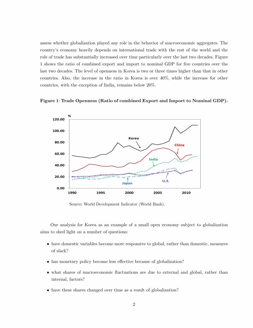
assess whether globalization played any role in the behavior of macroeconomic aggregates. The

country’s economy heavily depends on international trade with the rest of the world and the

role of trade has substantially increased over time particularly over the last two decades. Figure

1 shows the ratio of combined export and import to nominal GDP for five countries over the

last two decades. The level of openness in Korea is two or three times higher than that in other

countries. Also, the increase in the ratio in Korea is over 40%, while the increase for other

countries, with the exception of India, remains below 20%.

Figure 1: Trade Openness (Ratio of combined Export and Import to Nominal GDP).

0.00

20.00

40.00

60.00

80.00

100.00

120.00

1990 1995 2000 2005 2010

%

Korea

China

India

JapanU.S.

Source: World Development Indicator (World Bank).

Our analysis for Korea as an example of a small open economy subject to globalization

aims to shed light on a number of questions:

• have domestic variables become more responsive to global, rather than domestic, measures

of slack?

• has monetary policy become less effective because of globalization?

• what shares of macroeconomic fluctuations are due to external and global, rather than

internal, factors?

• have these shares changed over time as a result of globalization?

2

To answer to those questions, we use a structural approach by exploiting and estimating a

small open economy model, which includes several features that have been shown necessary in

fitting aggregate time series data in both closed and open-economy frameworks, such as habit

formation in consumption, sticky prices, indexation to past inflation, and so forth.

As a departure from conventional estimations, we relax the assumption of rational expecta-

tions, which is standard in open-economy macroeconomics. In a changing economy, the informa-

tional assumptions required by rational expectations would be exceedingly strong (i.e., agents

would be required to optimize taking into account changes in future openness: this complicates

the microfoundations and it doesn’t seem realistic), more so than in typical constant-parameter

environments. We instead model expectations as near-rational, and allow private-sector agents

to learn over time the relevant economic relationships. In the spirit of the macroeconomic adap-

tive learning literature (e.g., Evans and Honkapohja (2003)), we constrain agents in the model

to have no information advantage over the researchers and econometricians working with the

model (i.e., if econometricians do not observe the shocks and the model parameters, neither do

the agents in the model).

Moreover, given the plethora of evidence against the existence of financial market complete-

ness at the international level, we assume incomplete international financial markets. Among

other things, this assumption allows us to attenuate the restrictions imposed by the uncovered

interest parity condition on exchange rate fluctuations, by allowing for a debt-elastic interest

rate premium.

The structural small open economy model is estimated using full-information Bayesian

methods. The coefficients in the state-space representation of the model are time-varying because

they are a function of the degree of openness in the economy, which is itself time-varying and

is the key channel exploited here to model globalization, and also because of economic agents’

gradual learning about the economy.

Results Overview. The empirical results reveal the significant effects that globalization

has had on business cycle dynamics in Korea. The relationships among the major domestic and

foreign variables have crucially changed. Korean output has become progressively more sensitive

to global output and less dependent on domestic consumption. Domestic inflation is also driven to

a large extent by global, rather than exclusively domestic, slack. The influence of open-economy

variables, such as the terms of trade and exchange rate or risk premium shocks, has risen over

the sample. These developments are clearly exemplified by a variance decomposition exercise.

While domestic shocks to preferences, technology, and monetary policy account for more than

70% of business cycle fluctuations at the beginning of the 1990s, the situation is reversed as it is

external shocks (either global variables or variables related to open economy in nature such as

the terms of trade or exchange rates) that come to dominate by the end of the sample. Those

3

explain roughly 70% of the observed variability in output, inflation, and interest rates.

Related Literature. At the broadest level, this paper aims to contribute to our under-

standing of the changes in the structure and dynamics of economies that are brought by the

process of globalization. While economists have focused a large deal of attention on globalization

as a potential cause of the increase in wage inequality between high-skilled and low-skilled work-

ers, research on its implications for business cycle dynamics has been less common. As discussed

above, the papers that looked at the potential effects of globalization with a more macroeco-

nomic focus emphasized how globalization could change the dynamics of inflation, by making it

more a function of global, rather than domestic, measures. This paper contributes to this line of

research by providing evidence from a country that has been potentially more sensitive to the

forces of globalization.

On a methodological level, the paper presents an estimation of a microfounded small open

economy model, which departs from conventional estimations in the literature in two main

respects: first, it incorporates globalization, modeled in a highly tractable way, as a time-varying

structural parameter; and second, it departs from the assumption of rational expectations, which

can be unrealistically strong for economies that have moved from emerging to developed, and

have been subject to major structural changes over the period. As the estimation recognizes the

difficulties economic agents face in forming expectations in real time, it models expectations as

non-fully rational (although still close to rational), but also allows agents to progressively learn

about the economy.

At a more specific level, the paper provides an empirical investigation of the Korean econ-

omy, which reveals major changes in its characteristics over time. There are several studies that

address how the Korean economy is affected by external shocks or foreign factors. These papers

generally show that the business cycle in Korea is influenced by external shocks, although domes-

tic monetary policy still remains effective. For example, Kim and Park (2009) and Kim (2011)

use SVAR and find that output and inflation rate in Korea are affected by external shocks. Kang

and Mook (2009) claim, based on the results from Factor-Augmented VARs, that monetary pol-

icy in Korea is still effective even though domestic economic variables are unilaterally affected

by foreign factors. These studies, however, neither show how the effects of foreign factors on

business cycles in Korea change over time, nor explicitly deal with globalization.

2 Small Open Economy Model

The model is based on the small-open economy environments developed in Monacelli (2005),

and Galı and Monacelli (2005). The version used in the paper mirrors the model with incomplete

markets and endogenous sources of persistence, which is estimated in Justiniano and Preston

4

(2010a).1 We only present a sketch of the main features of the model here. The reader is referred

to the original papers for a detailed derivation.

2.1 Model Description

2.1.1 Households

Households derive utility from their total consumption Ct, in deviation from a stock of

consumption habits that they have accumulated up to that period, and they suffer disutility

from hours of labor supplied Nt. They are assumed to maximize

E0

∞∑t=0

βtζt

[(Ct − hCt−1)1−σ

1− σ− N1+ϕ

t

1 + ϕ

]. (1)

The parameters 0 ≤ β ≤ 1, 0 ≤ h ≤ 1, σ > 0, and ϕ > 0, denote the household’s

discount factor, the degree of (external) habit formation in consumption, and the inverse of

the elasticities of intertemporal substitution in consumption and of labor supply. The term ζt

represents an exogenous aggregate preference (or taste) shock, which can be interpreted, for

example, as a disturbance to the degree of consumers’ impatience.

The aggregate consumption term that enters households’ utility function is a composite

index of the Dixit-Stiglitz aggregates, CH,t and CF,t, of domestically and foreign-produced goods:

Ct =

[(1− α)1/ηC

η−1η

H,t + α1/ηCη−1η

F,t

] ηη−1

, (2)

where 0 ≤ α ≤ 1 denotes the share of foreign goods in the consumption basket and is typically

interpreted as the degree of openness of the domestic economy, and where η > 0 denotes the

elasticity of substitution across domestic and foreign goods. The aggregate indexes CH,t and

CF,t are given by

CH,t =

[∫ 1

0CH,t(j)

ε−1ε dj

] εε−1

, (3)

CF,t =

[∫ 1

0CF,t(j)

ε−1ε dj

] εε−1

, (4)

where ε > 1 indicates the elasticity of substitution across differentiated goods, produced either

domestically or abroad.

1Similar models, under rational expectations and constant openness, have been estimated in Kam et al. (2009),

Justiniano and Preston (2010b), and Beltran and Draper (2008), among several others.

5

Households maximize Equation (1) subject to a budget constraint, which is given in any

period by

PtCt +Bt + ΞtB∗t = (1 + it−1)Bt−1 + (1 + i∗t−1)φt(At)ΞtB

∗t−1 +WtNt + ΠH,t + ΠF,t + Tt, (5)

where Pt denotes the aggregate price level, Bt holdings of domestic (one-period) bonds, B∗t

holdings of foreign (one-period) bonds, Wt the nominal wage, ΠH,t and ΠF,t profits distributions

obtained from the ownership of domestic and foreign firms, and Tt lump-sum taxes or transfers.

International financial markets are incomplete, since investors have access only to domestic and

foreign one-period bonds, rather than to the full set of Arrow-Debreu securities. Domestic bonds

yield the interest rate it, while foreign bonds yield the interest rate i∗t and their rate of return

also depends on the (nominal) exchange rate Ξt and on the interest-rate (risk) premium φt(At),

which is assumed to be a positive function of the country’s level of foreign debt as a fraction of

steady-state output Y , and is modeled as

φt = exp[−χ(At + φt)

], (6)

At ≡Ξt−1Bt−1

Y Pt−1, (7)

where φt denotes the exogenous component of the risk-premium. Households allocate consump-

tion expenditures for each differentiated consumption good j, and across domestic and foreign

goods, according to the demand functions as below

CH,t(j) = (PH,t(j)/PH,t)−εCH,t, (8)

CF,t(j) = (PF,t(j)/PF,t)−εCF,t, (9)

CH,t(j) = (1− α)(PH,t/Pt)−ηCt, (10)

CF,t(j) = α(PF,t/Pt)−ηCt, (11)

where PH,t and PF,t denote aggregate price indexes corresponding to domestic and foreign con-

sumption baskets, and Pt = [(1−α)P 1−ηH,t +αP 1−η

F,t ]1/(1−η) is the consumer price index (CPI). The

elasticity across differentiated goods ε is allowed to differ from the elasticity between domestic

and foreign goods η.

The intratemporal and intertemporal optimality conditions are given by the following:

λt = ζt(Ct − hCt−1)−σ−1, (12)

λt = ζtPtNϕt /Wt, (13)

6

λt = Et

[β(1 + i∗t )φt+1λt+1

Ξt+1

ΞtΠt

], (14)

λt = Et [β(1 + it)λt+1Πt] , (15)

where Πt ≡ Pt/Pt−1 denotes the gross inflation rate, and λt denotes the Lagrange multiplier.

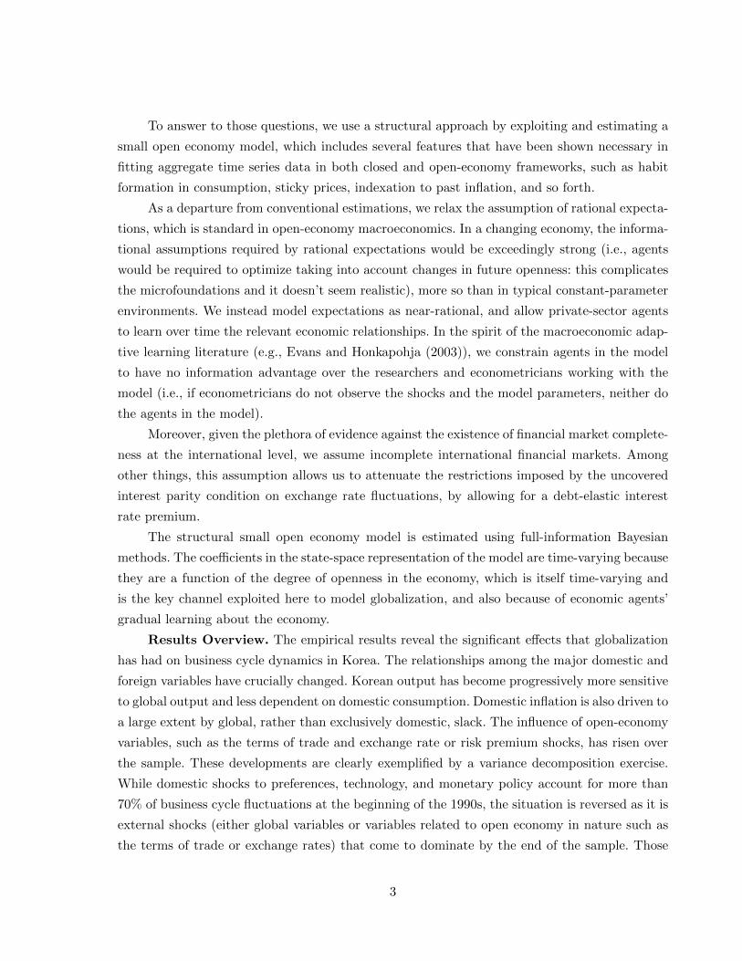
2.1.2 Firms

A continuum of domestic firms produce differentiated goods under monopolistic competition.

Prices are sticky a la Calvo: only a fraction 1 − θH of firms can set prices optimally in a given

period; the remaining fraction θH is not allowed to reoptimize its pricing plans and simply

adjusts prices based on the past period’s inflation rate πH,t−1, as follows

logPH,t(j) = logPH,t−1(j) + γHπH,t−1, (16)

where 0 ≤ γH ≤ 1 denotes the degree of inflation indexation. Firms maximize the expected

discounted sum of future profits

Et

∞∑T=t

θT−tH Qt,TYH,T (j)

[PH,t(j)

(PH,T−1

PH,t−1

)γH− WT

εa,t

], (17)

where εa,t denotes a technology disturbance, and YH,T (j) =(PH,t(j)PH,T

(PH,T−1

PH,t−1

)γH)−ε(CH,T +

C∗H,T ) is the demand curve that firms face for their product. The term PH,t, the aggregate

domestic price level, evolves as

PH,t =

[(1− θH)P

∗(1−ε)H,t + θH

(PH,t−1

(PH,t−1

PH,t−2

)γH)1−ε] 1

1−ε

. (18)

Besides domestic producers, the economy is populated by retail firms, which import foreign

differentiated goods and are also assumed to act as monopolistic competitors and, hence, enjoy

pricing power. Even though, following Monacelli (2005), the law of one price holds at the docks,

their pricing power leads to the law of one price deviations in the short run and to incomplete

exchange rate pass-through. Importing firms also set prices a la Calvo, with fractions 1−θF and

θF optimizing or setting prices according to the indexation rule (with degree of indexation now

denoted by γF ) each period. Importing firms maximize profits

Et

∞∑T=t

θT−tF Qt,TCF,T (j)

[PF,t(j)

(PF,T−1

PF,t−1

)γF− ΞTP

∗F,T (j)

](19)

subject to the demand curve CF,T (j) =(PF,t(j)PF,T

(PF,T−1

PF,t−1

)γF )−εCF,T .

7

The first-order conditions implied by profit maximization for domestic and importing firms

are given by

Et

∞∑T=t

θT−tH Qt,TYH,T (j)

[PH,t(j)

(PH,T−1

PH,t−1

)γH− ε

ε− 1

WT

εa,t

]= 0, (20)

Et

∞∑T=t

θT−tF Qt,TCF,T (j)

[PF,t(j)

(PF,T−1

PF,t−1

)γF− ε

ε− 1ΞTP

∗F,T (j)

]= 0. (21)

2.1.3 Exchange Rate, Terms of Trade, Monetary Policy

Exchange rate dynamics in the model are determined by the following uncovered interest

rate parity condition

Etλt+1Pt+1

[(1 + it)− (1 + i∗t )(

Ξt+1

Ξt)φt+1

]= 0. (22)

The condition typically restricts the differential between domestic and foreign interest rates to

equal the expected depreciation of the domestic currency. In our model, given the assumption of

incomplete markets, there can be a wedge in the relation, given by the risk-premium disturbance

φt.

The real exchange rate in the model is expressed as

Qt = ΞtP ∗tPt. (23)

As in Monacelli (2005), the law of one price may not hold at all times: the law of one price gap

may hence be defined as EtP ∗tPF,t6= 1. The terms of trade are defined as:

St =PF,tPH,t

. (24)

Given that the available data on the terms of trade for most countries do not exactly

match the definition in the model, in the empirical analysis, we take two approaches: in the first

approach, we exploit terms of trade data in the estimation and account for possible misalignments

by adding an exogenous disturbance εs,t (which can be alternatively interpreted as measurement

error); in the second approach, we force the terms of trade to match the definition in the model

and do not use a corresponding observable in the estimation (in such a case, we also omit the

shock). The overall empirical conclusions are similar in the two cases.

We assume that monetary policy in the home country is well approximated by the following

Taylor rule

8

it = ρit−1 + (1− ρ) [ψππt + ψyyt + ψe,t∆et] + εmp,t, (25)

which assumes that the Bank of Korea changes policy rates to react to fluctuations in domestic

output, to inflation, and to the growth rate of nominal exchange rates. The rule allows for

interest-rate smoothing in policy decisions. The term εmp,t accounts for unsystematic deviations

from the historical policy rule.

Finally, market clearing implies

YH,t = CH,t + C∗H,t, (26)

Y ∗t = C∗t . (27)

2.2 Model Summary

The model’s optimality and equilibrium conditions are log-linearized around a non-stochastic

steady state. The resulting log-linearized equations used in the empirical analysis are shown

below:

ct =h

1 + hct−1 +

1

1 + hEtct+1 −

1− hσ(1 + h)

(it − Etπt+1

)+

(1− h)(1− ρζ)σ(1 + h)

εζ,t, (28)

yt = (1− αt)ct + αtη (qt + st) + αty∗t , (29)

πt = (1− αt)πH,t + αtπF,t, (30)

πH,t =β

1 + βγHEtπH,t+1 +

γH1 + βγH

πH,t−1 +

+λH

1 + βγH

[ϕyt − (1 + ϕ)εa,t + αtst + qt +

σ

1− h(ct − hct−1)

], (31)

πF,t =β

1 + βγFEtπF,t+1 +

γF1 + βγF

πF,t−1 +λF

1 + βγF[qt − (1− αt)st] + εcp,t, (32)

et − et−1 = qt − qt−1 + πt − π∗t , (33)

Etet+1 − et = it − i∗t + χat + εφ,t, (34)

at = β−1at−1 − αt (qt + αtst)−αt

1− αtyt +

αt1− αt

[η (st + qt) + y∗t ] , (35)

st − st−1 = πF,t − πH,t + εs,t, (36)

it = ρit−1 + (1− ρ) [ψππt + ψyyt + ψe,t∆et] + εmp,t. (37)

The Equation (28) is the Euler equation for consumption under habit formation in con-

sumers’ preferences. The goods market clearing condition, expressed by Equation (29), posits

9

a relation between domestic output and domestic consumption, the terms of trade, the real

exchange rate, and global output. Equations (30) to (32) define the dynamics of inflation: CPI

inflation is a weighted average of domestic and import-price inflation. Domestic inflation evolves

according to a New Keynesian Phillips curve, with the current inflation rate driven by expected

future inflation, lagged inflation, and current marginal costs. Marginal costs in the equation are

a function of current output, technology shocks, the terms of trade, the real exchange rate, and

current and lagged consumption. Import price inflation is driven by expectations, lagged terms,

and the law of one price gap, which depends on the real exchange rate and on the terms of

trade. The composite coefficients λH and λF , which define the slope of the Phillips curves, are

negative functions of the degrees of price stickiness θH and θF , respectively.

Equation (33) defines the real exchange rate: changes in the nominal exchange rate equal

changes in the real exchange rate plus changes in domestic inflation minus changes in foreign

inflation. The main equation for the determination of exchange rates in the model is given by

the log-linearized UIP condition (34): the expected depreciation of the nominal exchange rate

equals the differential between home and foreign interest rates, but, given the assumption of

incomplete markets, it also depends on the country’s financial assets position and on the risk-

premium shock εφ,t. Net foreign assets evolve according to equation (35). Equation (36) defines

the terms of trade: quarterly changes are equal to the differential between foreign-produced and

domestic-produced-goods inflation; this is not a perfect equality, however, as we allow, at least

for now, for a shock, which is meant to capture misalignments between the available data on

the terms of trade and the implied theoretical variable in the model.

The final equation (37) represents a Taylor rule for an open economy. The policy rate is

adjusted gradually in reaction to movements in inflation, output, and (nominal) exchange rates.

Given that the exchange rate regime in Korea switches from a managed float arrangement to a

floating regime in 1997, we allow for a break in the response coefficient to exchange rates.2

In the model, we replaced the mathematical expectation operator Et with the more flexible

subjective expectation indicator Et. The next subsection describes how such expectations are

formed. Moreover, we let the openness parameter α be time-varying in the empirical section to

match the increase in openness in Korea over the period.

The global, or the rest of the world (ROW), variables (y∗t , π∗t , i∗t collected in vector X∗t ),

which enter some of the main structural equations, are modeled in an unrestricted fashion as

following a VAR(1):

X∗t = zX∗t−1 + Ωε∗t , (38)

2Taylor rules with high response coefficients to exchange rates represent a straightforward way to model actively

managed or fixed exchange rate regimes.

10

where the matrix z contains the VAR coefficient f11, ..., f33 and Ω is assumed to be diagonal.3

There is a total of nine structural disturbances in the model: the domestic preference,

technology, cost-push, monetary policy, the terms of trade, the exchange rate or interest rate

risk premium, global output, global inflation, and global interest rate shocks.

2.3 Non-Fully Rational Expectations

We relax the strong informational assumptions implicit in the rational expectations hypoth-

esis. The deviation from rational expectations is, however, kept small: the assumed expectation

formation model is typically interpreted as ‘near’-rational. Agents are assumed to form forecasts

based on their Perceived Law of Motion (PLM), which has the same structural form as the Min-

imum State Variable (MSV) solution of the system under rational expectations. For empirical

realism, we assume that agents observe historical data related to the model’s endogenous vari-

ables, but they are unable to observe the structural disturbances. Such an assumption is meant

to endow agents with a level of knowledge that doesn’t surpass the knowledge of an economic

researcher or econometrician working with the model. The agents’ PLM is given by

Yt = at + btYt−1 + εt, (39)

where at is a vector of estimated intercepts, bt is a matrix of coefficients describing the perceived

dynamics of the economy, and Yt = [ct, πt, πH,t, πF,t, qt, st, it, at, et, y∗t , π∗t , i∗t ]′. Therefore, we allow

economic agents in the small open economy to incorporate information on foreign variables to

form their expectations. The PLM is written in its more general form, but it is necessary to point

out that some coefficients are equal to zero: the coefficients on lagged CPI inflation are equal to

zero (as they are zero in the MSV solution under RE), while the coefficients on its components,

domestic and import price inflation are non-zero. Also, as under rational expectations, domestic

agents recognize that global output, inflation, and interest rates are exogenous to the domestic

economy (the small open economy assumption): in the perceived equations for these global

variables, the coefficients on domestic variables are restricted to zero.

Agents estimate the PLM using the available historical time series at each point in time.

They update their beliefs according to the learning formulae

φt = φt−1 + gR−1t Xt(Yt −X ′tφt−1), (40)

Rt = Rt−1 + g(XtX′t −Rt−1), (41)

3We restrain from modeling the rest of the world aggregate in a structural fashion, given the heterogeneity of

the economies it includes. The aggregate dynamics of global variables are well represented empirically by an

atheoretical VAR.

11

where φt = [at, bt]′ and Xt = [1, Y ′t−1]′. The first expression describes the updating of mean

beliefs φt (i.e., the perceived coefficients), which collect all the relevant coefficients in at and bt,

and the second the updating of the associated precision matrix Rt. Agents’ expectations formed

from equation (39), which are updated via equations (40) and (41), can be substituted into the

system expressed by equations (28)-(38) to yield the so-called economy’s Actual Law of Motion

or ALM.

3 Estimation Details

3.1 State Space

The ALM of the model can be inserted in a state-space system and written as

ξt = At

(αt, φt

)+ Ft

(αt, φt

)ξt−1 +Gt

(αt, φt

)ωt (42)

Observablest = Hξt (43)

where ξt collects the model’s endogenous variables, the structural disturbances, and the ex-

pectation terms, and ωt collects the structural innovations. The second equation in the system

represents the set of measurement equations linking observables with their counterparts in the

model, through the selection matrix H.

The vectors and matrices of coefficients A, F , and G in the ALM are functions of the degree

of openness in the economy, measured by the parameter αt, which is varying over time because

of increased globalization. Figure 2 shows the degree of openness αt over the sample. They are

also time-varying because of private-sector agents’ learning and evolving beliefs summarized by

φt.

The structural parameter αt affects the dynamic interactions between the variables in the

system and, in particular, the extent to which domestic conditions are sensitive to open-economy

and foreign variables. By allowing for the structure of the economy to depend on the time-varying

αt, we are able to investigate the impact of globalization on macroeconomic dynamics in Korea.

3.2 Data

We estimate the structural small open economy model using quarterly data for Korea and

global variables for a sample spanning the period between 1991:I and 2012:IV. In the estimation

we match the following set of observables (corresponding to the variable in the model in paren-

thesis): Korea data for real GDP (yt), the CPI inflation rate (πt), import price inflation (πF,t),

12

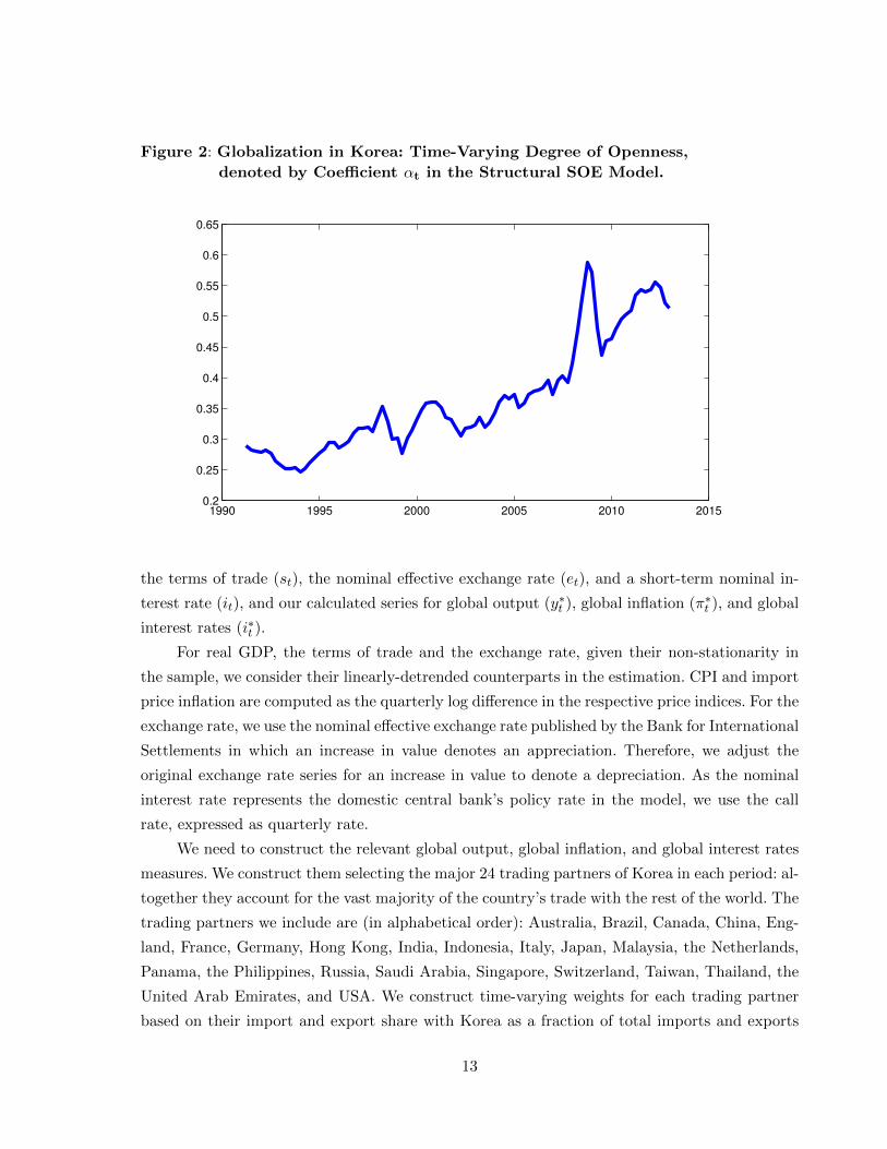
Figure 2: Globalization in Korea: Time-Varying Degree of Openness,

denoted by Coefficient αt in the Structural SOE Model.

1990 1995 2000 2005 2010 20150.2

0.25

0.3

0.35

0.4

0.45

0.5

0.55

0.6

0.65

the terms of trade (st), the nominal effective exchange rate (et), and a short-term nominal in-

terest rate (it), and our calculated series for global output (y∗t ), global inflation (π∗t ), and global

interest rates (i∗t ).

For real GDP, the terms of trade and the exchange rate, given their non-stationarity in

the sample, we consider their linearly-detrended counterparts in the estimation. CPI and import

price inflation are computed as the quarterly log difference in the respective price indices. For the

exchange rate, we use the nominal effective exchange rate published by the Bank for International

Settlements in which an increase in value denotes an appreciation. Therefore, we adjust the

original exchange rate series for an increase in value to denote a depreciation. As the nominal

interest rate represents the domestic central bank’s policy rate in the model, we use the call

rate, expressed as quarterly rate.

We need to construct the relevant global output, global inflation, and global interest rates

measures. We construct them selecting the major 24 trading partners of Korea in each period: al-

together they account for the vast majority of the country’s trade with the rest of the world. The

trading partners we include are (in alphabetical order): Australia, Brazil, Canada, China, Eng-

land, France, Germany, Hong Kong, India, Indonesia, Italy, Japan, Malaysia, the Netherlands,

Panama, the Philippines, Russia, Saudi Arabia, Singapore, Switzerland, Taiwan, Thailand, the

United Arab Emirates, and USA. We construct time-varying weights for each trading partner

based on their import and export share with Korea as a fraction of total imports and exports

13

with the selected set of partners in each period. In the few cases in which observations on GDP,

inflation, or interest rates for the trading partner are not available in a given quarter (which

happens for some countries in the early part of the sample), we assign them a zero weight and,

hence, exclude them from the computation of the relevant global measure in that period. The

impact of occasional missing data on the results should be minimal, given that data are available

for the major trading partners (USA, Japan, China, Germany, etc.).

Given that we consider linearly detrended domestic GDP, we use the same detrending

procedure for global GDP. We linearly detrend real GDP series for each trading partner using

the available samples. Global inflation are computed as the quarterly log difference in the price

index and interest rates are considered in levels (as quarterly rates). We choose seasonally

adjusted data when available and, when they are not, we run the seasonal adjustment procedure

on the raw series (except for interest rates). Global measures are computed as weighted averages

as:

y∗t =

N∑j=1

wy,jt yjt , (44)

π∗t =N∑j=1

wπ,jt πjt , (45)

i∗t =N∑j=1

wi,jt ijt , (46)

where j = 1, ..., N , N = 24, is an index for the different trading partners, yjt , πjt , and ijt are the

detrended output, inflation rate, and short-term interest rate, of trading partner j, and where

the weights wz,jt , for variable z = y, π, i, are given in each period t by the sum of Korea’s imports

and exports with country j, as a fraction of total Korean imports and exports with the set of

trading partners:4

wz,jt =(Importsjt + Exportsjt )∑Ni=1(Importsjt + Exportsjt )

. (47)

Figure 3 shows the resulting series for (detrended) global output, global inflation, and

global interest rates, along with the six domestic variables used in the estimation. The global

4The only reason why the weights may differ across variables is because possibly different observations may be

missing for GDP, inflation, or interest rates, for the different countries. As discussed before, when an observation

for a country is missing, that country is assigned a zero weight in the computation of the global measure in that

period.

14

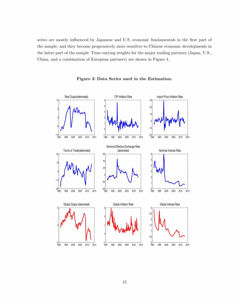
series are mostly influenced by Japanese and U.S. economic fundamentals in the first part of

the sample, and they become progressively more sensitive to Chinese economic developments in

the latter part of the sample. Time-varying weights for the major trading partners (Japan, U.S.,

China, and a combination of European partners) are shown in Figure 4.

Figure 3: Data Series used in the Estimation.

1990 1995 2000 2005 2010 2015−10

−5

0

5

10

Real Output(detrended)

1990 1995 2000 2005 2010 2015−1

0

1

2

3

4

5

CPI Inflation Rate

1990 1995 2000 2005 2010 2015−20

−10

0

10

20

30

Import Price Inflation Rate

1990 1995 2000 2005 2010 2015−20

−10

0

10

20

Terms of Trade(detrended)

1990 1995 2000 2005 2010 2015−40

−20

0

20

40

60

Nominal Effective Exchange Rate(detrended)

1990 1995 2000 2005 2010 20150

1

2

3

4

5

6

Nominal Interest Rate

1990 1995 2000 2005 2010 2015−5

0

5

Global Output (detrended)

1990 1995 2000 2005 2010 2015−1

0

1

2

3

Global Inflation Rate

1990 1995 2000 2005 2010 20150

0.5

1

1.5

2

2.5

3

Global Interest Rate

15

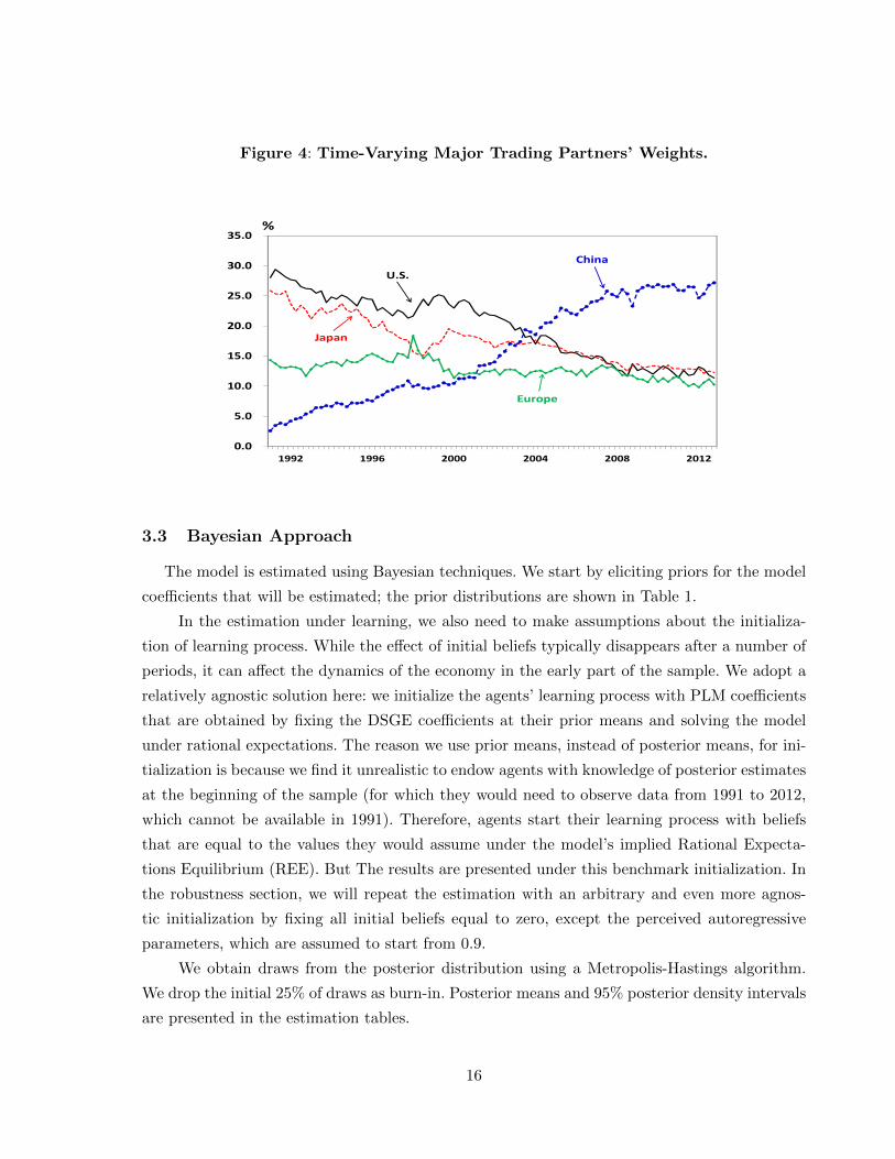
Figure 4: Time-Varying Major Trading Partners’ Weights.

0.0

5.0

10.0

15.0

20.0

25.0

30.0

35.0

1992 1996 2000 2004 2008 2012

U.S.

Japan

China

Europe

%

3.3 Bayesian Approach

The model is estimated using Bayesian techniques. We start by eliciting priors for the model

coefficients that will be estimated; the prior distributions are shown in Table 1.

In the estimation under learning, we also need to make assumptions about the initializa-

tion of learning process. While the effect of initial beliefs typically disappears after a number of

periods, it can affect the dynamics of the economy in the early part of the sample. We adopt a

relatively agnostic solution here: we initialize the agents’ learning process with PLM coefficients

that are obtained by fixing the DSGE coefficients at their prior means and solving the model

under rational expectations. The reason we use prior means, instead of posterior means, for ini-

tialization is because we find it unrealistic to endow agents with knowledge of posterior estimates

at the beginning of the sample (for which they would need to observe data from 1991 to 2012,

which cannot be available in 1991). Therefore, agents start their learning process with beliefs

that are equal to the values they would assume under the model’s implied Rational Expecta-

tions Equilibrium (REE). But The results are presented under this benchmark initialization. In

the robustness section, we will repeat the estimation with an arbitrary and even more agnos-

tic initialization by fixing all initial beliefs equal to zero, except the perceived autoregressive

parameters, which are assumed to start from 0.9.

We obtain draws from the posterior distribution using a Metropolis-Hastings algorithm.

We drop the initial 25% of draws as burn-in. Posterior means and 95% posterior density intervals

are presented in the estimation tables.

16

Table 1: Prior Distributions and Posterior Estimates, Baseline Model.

Parameters Prior Distributions Posterior Mean 95% PDI

η Γ(2, 0.25) 0.47 [0.36, 0.60]

h B(0.7, 0.1) 0.70 [0.48, 0.85]

σ Γ(1.5, 0.25) 1.40 [0.92, 1.91]

γH B(0.7, 0.1) 0.64 [0.40, 0.83]

θH B(0.75, 0.1) 0.82 [0.61, 0.93]

ϕ Γ(1.5, 0.125) 1.52 [1.29, 1.75]

γF B(0.7, 0.1) 0.51 [0.27, 0.77]

θF B(0.75, 0.1) 0.29 [0.23, 0.35]

χ Γ(0.01, 0.005) 0.009 [0.003, 0.02]

ρ B(0.7, 0.1) 0.83 [0.78, 0.89]

ψπ N(1.5, 0.125) 1.63 [1.40, 1.86]

ψy N(0.25, 0.125) 0.11 [0.02, 0.22]

ψ∆e,≤97 Γ(0.75, 0.3) 0.39 [0.23, 0.62]

ψ∆e,≥98 Γ(0.15, 0.15) 0.13 [0.05, 0.27]

ρz B(0.5, 0.2) 0.33 [0.14, 0.53]

ρa B(0.5, 0.2) 0.23 [0.06, 0.58]

ρcp B(0.5, 0.2) 0.79 [0.67, 0.90]

ρs B(0.5, 0.2) 0.68 [0.50, 0.81]

ρφ B(0.5, 0.2) 0.33 [0.16, 0.52]

σz Γ−1(0.5, 2) 3.84 [3.17, 4.75]

σa Γ−1(0.5, 2) 1.14 [0.94, 1.48]

σcp Γ−1(0.5, 2) 8.72 [7.04, 10.88]

σs Γ−1(0.5, 2) 6.57 [5.66, 7.61]

σφ Γ−1(0.5, 2) 8.85 [7.75, 10.13]

σmp Γ−1(0.5, 2) 0.29 [0.25, 0.33]

f11 B(0.8, 0.1) 0.94 [0.87, 0.98]

f12 N(0, 0.25) -0.09 [-0.34, 0.15]

−f13 Γ(−0.25, 0.15) 0.14 [0.03, 0.30]

f21 Γ(0.1, 0.05) 0.05 [0.02, 0.09]

f22 B(0.5, 0.2) 0.53 [0.35, 0.71]

f23 N(0, 0.25) 0.07 [-0.15, 0.28]

f31 Γ(0.1, 0.05) 0.04 [0.02, 0.09]

f32 Γ(0.1, 0.05) 0.06 [0.02, 0.11]

f33 B(0.8, 0.1) 0.78 [0.67, 0.88]

σy∗ Γ−1(0.5, 1) 0.85 [0.72, 0.99]

σπ∗ Γ−1(0.5, 1) 0.50 [0.43, 0.59]

σi∗ Γ−1(0.5, 1) 0.21 [0.18, 0.25]

g B(0.025, 0.005) 0.009 [0.006, 0.012]

Note: Γ denotes Gamma distribution, B Beta distribution, N Normal distribution,

and Γ−1 Inverse Gamma distribution. The prior distributions are expressed

in terms of mean and standard deviation.

17

4 Results

4.1 Structural Estimates

Table 1 reports the posterior estimates for the baseline model. There is typically a large

uncertainty in the literature on the values assumed by η, the elasticity of substitution across

domestic and foreign goods, with values ranging from close to zero (particularly in estimations)

to much higher (in calibrations). Here, we find a posterior mean estimate equal to 0.47, which is

in line with many estimates for other countries, although lower than typical calibration choices.

Regarding nominal rigidities, there is substantial evidence of price stickiness for firms producing

domestic goods, with a mean for the Calvo coefficient θH equal to 0.82; the degree of stickiness

in the import sector is, instead, quite limited, with a Calvo coefficient θF estimated at 0.29.

Such value implies a non-trivial, although imperfect, degree of exchange-rate pass-through.

The posterior estimates regarding the Bank of Korea’s monetary policy rule indicate an

aggressive response toward fluctuations in CPI inflation (ψπ = 1.63), a more limited response

to real activity (ψy = 0.11). The estimates also signal an attention toward exchange rate move-

ments, with a reaction coefficient to the growth rate of the nominal exchange rate ψ∆e that

shifts from 0.39 in the managed float pre-crisis period to 0.13 after 1997 (the latter obtained

under a prior distribution favoring values close to zero).

The persistence of the structural disturbance hitting the economy is not extreme: the

autoregressive coefficients are estimated at values between 0.23 and 0.79. The shocks, however,

have a high volatility, and particularly so the open-economy shocks to import price, the terms

of trade, and the risk premium.

Finally, we have also estimated the constant gain coefficient, which is responsible for gov-

erning the speed at which agents learn about the structure of the economy, along with the other

‘deep’ parameters of the model. We find a posterior mean for the constant gain equal to 0.009,

with a value that is somewhat smaller than the ones typically found for the U.S. (e.g., Milani

(2007), Milani (2011)).

4.2 Globalization and Macroeconomic Dynamics

As a result of globalization, the relationships between macroeconomic variables in Korea and

in the rest of the world may change in magnitude over the sample. Figure 5 shows the implied

reduced-form coefficients, i.e. the relevant elements in the matrix Ft(αt, φt), describing some of

the most interesting relationships. For each panel, the figure shows the posterior mean estimate

18

of the composite reduced-form coefficient over the sample, along with the 5% and 95% bands.

The main change which is apparent from the figure is that Korea’s output has become much

more responsive to global measures of slack over time, as yt has become more and more driven

by y∗t , and less influenced by domestic demand, with the effect of domestic consumption on

output falling over time. The effect of open-economy variables, as the terms of trade and the

real exchange rate, on real activity has also increased over the sample.

Figure 5: Time-Varying Reduced-Form Coefficients.

1990 1995 2000 2005 2010 20150

0.2

0.4

0.6

0.8

1

Effect of y* on y

1990 1995 2000 2005 2010 20150.1

0.2

0.3

0.4

0.5

0.6

Effect of c on y

1990 1995 2000 2005 2010 20150.05

0.1

0.15

0.2

0.25

0.3

0.35

0.4

Effect of y* on π

1990 1995 2000 2005 2010 20150

0.05

0.1

0.15

0.2

Effect of π* on π

1990 1995 2000 2005 2010 2015

0.2

0.25

0.3

0.35

0.4

0.45

0.5

Effect of i* on i

1990 1995 2000 2005 2010 20150.05

0.1

0.15

0.2

0.25

0.3

Effect of s on y

1990 1995 2000 2005 2010 20150.04

0.06

0.08

0.1

0.12

0.14

Effect of q on y

1990 1995 2000 2005 2010 20150.06

0.08

0.1

0.12

0.14

0.16

0.18

Effect of q on π

Note: The graphs show posterior means across draws for the composite reduced-form coefficients,along with 5% and 95% percentile bands.

The recent literature on globalization and the role of global slack for macroeconomics and

monetary policy has mostly focused on the increased significance of global slack as a driver of

domestic inflation rates. While the evidence for such countries as the U.S. is mixed, the evidence

is clearly more favorable for Korea: the dependence of πt on global output has risen from values

close to 0.09 to around 0.3 in 2012. The effect is also quite precisely estimated. Inflation also has

become more sensitive to exchange rates over time. The only relationship that doesn’t seem to

have consistently changed over time is the one between domestic and global inflation: we may

speculate that the estimated coefficient’s movement toward zero may be a consequence of the

overall stability of inflation rates around the world in the second part of the sample.

19

It is worth reminding that the reduced-form interactions in the economy are time-varying

not only as a result of globalization, but also as a result of the variation in agents’ beliefs due to

their incremental learning process about the economy. To separate the two influences, Figure 6

shows the previous time-varying coefficients along with the new counterfactual paths (shown in

red) that they would have followed if the globalization channel was shut down. In such a case,

the degree of openness in Korea’s economy is fixed at its value at the beginning of the sample

(roughly 28% in 1990) and not allowed to change afterwards. The graphs clearly show that the

dependence of Korean macroeconomic variables on their global counterparts would have been

significantly diminished, had globalization not taken place. Domestic output would be much

more dependent on domestic consumption than on global output (with coefficients moving from

0.7 to 0.4 for global output, and from 0.3 to 0.5 for consumption), the sensitivity of inflation

to global slack would be cut alomost in half, and the role of the terms of trade and the real

exchange rate in the economy would be scaled down.

Figure 6: Comparison of Time-Varying Reduced-Form Coefficients with and without

Globalization.

1990 1995 2000 2005 2010 20150

0.2

0.4

0.6

0.8

1

Effect of y* on y

1990 1995 2000 2005 2010 20150.1

0.2

0.3

0.4

0.5

0.6

Effect of c on y

1990 1995 2000 2005 2010 20150.05

0.1

0.15

0.2

0.25

0.3

0.35

0.4

Effect of y* on π

1990 1995 2000 2005 2010 20150

0.05

0.1

0.15

0.2

Effect of π* on π

1990 1995 2000 2005 2010 2015

0.2

0.25

0.3

0.35

0.4

0.45

0.5

Effect of i* on i

1990 1995 2000 2005 2010 20150.05

0.1

0.15

0.2

0.25

0.3

Effect of s on y

1990 1995 2000 2005 2010 20150.04

0.06

0.08

0.1

0.12

0.14

Effect of q on y

1990 1995 2000 2005 2010 20150.06

0.08

0.1

0.12

0.14

0.16

0.18

Effect of q on π

Note: The graphs show posterior means across draws for the composite reduced-form coefficients,along with 5% and 95% percentile bands. The red lines represent the counterfactualcoefficients that would be obtained in the same model, if globalization hadn’t taken place(α constant and fixed to its value in 1990).

20

4.3 The Role of Domestic and Global Shocks

Figure 7 displays a selection of impulse responses for the main variables of interest to domestic

and global shocks. The figure shows how the impulse responses vary across the sample period

from 1991:I to 2012:IV. The top-left panel in the Figure highlights one of the main changes

affecting the Korean economy over the sample: the response of domestic output to global output

shocks has constantly increased over the sample, and it is around two times larger in 2012 than

it was in 1991. Domestic real activity has also become more responsive to terms of trade and

exchange rate shocks (the top-right panel and the mid-left panel in the Figure).

The mid-right panel and the bottom-left panel in the Figure present the corresponding

evidence for inflation. Global output shocks have had a progressively larger effect on inflation

over the sample, with a peak response that increased from less than 0.1 in 1991 to 0.25 in 2012,

while domestic technology shocks have seen their effects halve over the period.

Finally, another noticeable change is that domestic nominal interest rates have become

much more reactive to shocks affecting global interest rates than they were in the earlier decades

(the bottom-right panel in the Figure).

A central source of interest in the impact of globalization on the macroeconomy is the

idea that globalization may hinder the effectiveness of domestic monetary policies when the

economy is influenced by global variables. We assess the evidence on changes in monetary policy

effectiveness by looking at the effects of exogenous monetary policy shocks over the sample.

Even though global conditions have progressively become more important, domestic monetary

policy in Korea has remained effective. Figure 8 clarifies that its effects remain very similar at

each point in the sample.

Given the importance of global variables and shocks documented so far, we can ask the

following, possibly more general, questions: what shares of business cycle, inflation, and interest

rate fluctuations in Korea are due to global, rather than domestic, forces? How much have these

shares changed over time as a consequence of globalization?

We answer these questions by presenting evidence from a (forecast error) variance de-

composition exercise. Figure 9 illustrates the variance shares of Korea’s output, consumption,

inflation, and interest rate that can be accounted for by global and domestic shocks.5 Given that

the variance decomposition results are also time-varying, the figure shows how the shares evolve

every quarter from 1991 to 2012.

Business cycle fluctuations at the beginning of the sample are mostly driven by domestic

5We adopt here a flexible definition of ”global” we include not only global shocks to world output, inflation, and

interest rates, but also shocks related to the country’s open-economy dimension, such as terms of trade, exchange

rate, and import cost-push shocks.

21

Figure 7: Time-Varying Impulse Responses

05

1015

20

19911995

20002005

2010

−0.5

0

0.5

1

Horizon

Domestic Output to Global Output Shock

Sample

Re

sp

on

se

05

1015

20

19911995

20002005

2010

−4

−2

0

2

Horizon

Domestic Output to Terms of Trade Shock

Sample

Re

sp

on

se

05

1015

20

19911995

20002005

2010

−2

0

2

4

Horizon

Domestic Output to Exchange−Rate Shock

Sample

Re

sp

on

se

05

1015

19911995

20002005

2010

−0.5

0

0.5

Horizon

Domestic Inflation to Global Output Shock

Sample

Re

sp

on

se

05

1015

19911995

20002005

2010

−2

−1

0

1

Horizon

Domestic Inflation to Technology Shock

Sample

Re

sp

on

se

05

1015

20

19911995

20002005

2010

−0.2

0

0.2

Horizon

Domestic Interest Rate to Global Interest Rate Shock

Sample

Re

sp

on

se

22

Figure 8: Time-Varying Effects of Monetary Policy

0

5

10

15

19911995

2000

2005

2010

−0.15

−0.1

−0.05

0

0.05

Horizon

Domestic Output to Monetary Policy Shock

Sample

Response

0

5

10

15

20

19911995

2000

2005

2010

−0.1

−0.08

−0.06

−0.04

−0.02

0

0.02

Horizon

Domestic Inflation to Monetary Policy Shock

Sample

Response

shocks (largely preference and technology shocks), which account for more than 70% of output

variability, with a limited role for global variables. The situation strongly reverses by the end

of the sample: now Korean business cycles are driven by global shocks (with a share equal to

70%), with a smaller role for domestic innovations.

As expected, consumption expenditures are still dominated by domestic shocks, mostly by

consumers’ preferences, but the influence of global drivers has rapidly increased over the sample,

accounting for almost half of the variance by the end of the sample.

The transforming impact of globalization is also evident in the evolution of the variance

decomposition shares for inflation and interest rates. While the variables are mainly driven by

domestic shocks in the early 1990s, the role of global shocks becomes dominant starting from

the late 1990s - early 2000s, and by 2012, global and open-economy-related shocks explain about

80% of inflation and interest rate fluctuations.

5 Robustness

To assess the sensitivity of our main results to some of the choices that have been made in

the empirical analysis, we repeat the estimation considering the following four modifications.

The posterior estimates under these robustness checks are shown in Table 2.

Initial Learning Beliefs. The first modification relates to the choice of initial beliefs for

the agents’ learning algorithm. Rather than assuming that they start with beliefs fixed at their

23

Figure 9: Forecase Error Variance Decomposition over Time

1990 1995 2000 2005 2010 20150.2

0.4

0.6

0.8

1Domestic Output

1990 1995 2000 2005 2010 20150

0.2

0.4

0.6

0.8

1Consumption

1990 1995 2000 2005 2010 20150

0.2

0.4

0.6

0.8

1Domestic Inflation

1990 1995 2000 2005 2010 20150

0.2

0.4

0.6

0.8

1Domestic Interest Rate

Note: The solid red line represents the share of variance explained by global (global output,global inflation, global interest rates, importing price, exchange rate and terms of trade)shocks while the dotted blue line represents the share of variance explained by domestic(techonology, preference, and monetary policy) shocks.

values in a REE obtained with the model’s coefficients equal to their prior means, we now

assume an uninformative, although ad hoc, initialization. We fix all initial beliefs, except the

coefficients of a variable on its own first lag, to be equal to zero. The autoregressive coefficients

are assumed to start at a value of 0.9 at the beginning of the sample in 1991. The values are

the same for each variable. Such initialization is somewhat in the spirit of Minnesota priors in

the VAR literature (although with 0.9 rather than 1 as first-lag coefficients) and it attempts to

capture the general ignorance of economic agents about the structure of the economy, with the

knowledge that macroeconomic time series are generally quite persistent.

Terms of Trade. Secondly, we change our treatment of the terms of trade variable. In

the benchmark estimation, we used data on the terms of trade, obtained as the log difference

between the price of exports and the price of imports, as one of the observable variables to match.

In the model, however, the terms of trade are given by the difference between πF,t and πH,t. By

using the empirical measure, instead, we have allowed for differences between the two through

the exogenous disturbance εs,t. An alternative, which we consider here, is to take the model at

heart, rather than using outside data, simply letting terms of trade equal to their definition in

24

the model. In this case, we have eight observables and eight shocks in the estimation, rather

than nine and nine. The empirical literature has been split about using the first or the second

approach regarding the terms of trade.

Post-1997 Sample. Given that the Korean economy is likely subject to a structural

break, at least in the monetary and exchange rate policy strategy in the aftermath of the 1997

financial crisis, we repeat the estimation on the shorter sample, now starting in 1998:I and ending

in 2012:IV. In this case, we do not need to assume a break in the feedback coefficient to the

nominal exchange rate in the Taylor rule.

Taylor Rule Dependence on Foreign Interest Rate. As a final sensitivity check, we

allow for monetary policy decisions to be influenced by the global monetary policy stance. In

this scenario, interest rate policies in the U.S., Japan, China, and the Euro area could have a

particular effect on Korea’s interest rates. We re-estimate the model using this version of the

Taylor rule

it = ρit−1 + ρ∗i∗t−1 + (1− ρ) [ψππt + ψyyt + ψe∆et] + εmp,t, (48)

where domestic interest rates can also respond to foreign interest rates through the reaction

coefficient ρ∗ (for which we assume a Beta(0.5,0.2) prior). For this case, we also restrict the

sample to the post-1997 period.

The posterior estimates regarding the robustness checks are reported in Table 2. Under the

non-informative learning initialization, the estimated elasticity of substitution between domestic

and foreign goods becomes larger. Non-fully rational beliefs and learning introduce more persis-

tence in the system in this case: the estimates of habit formation and of the persistence in the

terms of trade shock are reduced in this case. The situation is different when terms of trade data

are not exploited in the estimation: the elasticity of substitution is lower, while the habit for-

mation, the cost-push and exchange rate disturbance persistence parameters generally increase.

Given that the terms of trade disturbance is no longer present in the model, the volatility of the

cost-push shock rises with respect to the baseline case to help the model fitting the data despite

the tighter restrictions. The notable changes in the estimates in the post-1997 sample are that

the response to the exchange rate in the monetary policy rule is much closer to zero and the

volatility of the cost-push is much lower. There is some evidence of an effect of foreign interest

rates, although the magnitude of the response is small (ρ∗ = 0.11).

The table also reports the minimum and maximum shares of output due to the menu of

global shocks over the samples for the different specifications. The minimum shares also fall at

the beginning of the sample with values around 0.20-0.30, and the maximum values appear either

right before the financial crisis or in 2012 and attain values between 0.65 and 0.82. Therefore,

the overall conclusions do not substantially change under any of the previous alternatives.

25

Table 2: Posterior Estimates, Robustness Checks.

(Different Initial Beliefs) (No ToT data) (Post-1997) (MP Reaction to i∗)

Parameters Mean 95% PDI Mean 95% PDI Mean 95% PDI Mean 95% PDI

η 0.60 [0.37,0.92] 0.32 [0.24,0.43] 0.57 [0.40,0.75] 0.57 [0.41,0.79]

h 0.50 [0.22,0.78] 0.81 [0.64,0.91] 0.61 [0.43,0.78] 0.49 [0.24,0.73]

σ 1.00 [0.46,1.70] 1.43 [1.05,1.83] 1.29 [0.90,1.78] 1.12 [0.60,1.69]

γH 0.66 [0.45,0.85] 0.63 [0.42,0.83] 0.68 [0.42,0.86] 0.65 [0.47,0.85]

θH 0.54 [0.17,0.84] 0.78 [0.70,0.85] 0.57 [0.38,0.81] 0.64 [0.32,0.84]

ϕ 1.55 [1.33,1.81] 1.50 [1.28,1.77] 1.52 [1.29,1.77] 1.52 [1.28,1.81]

γF 0.64 [0.43,0.85] 0.57 [0.31,0.82] 0.64 [0.42,0.86] 0.66 [0.40,0.86]

θF 0.23 [0.18,0.29] 0.20 [0.13,0.27] 0.57 [0.38,0.81] 0.48 [0.30,0.67]

χ 0.01 [.003,0.02] 0.009 [.002,0.02] 0.006 [.003,0.01] 0.011 [.004,0.03]

ρ 0.80 [0.71,0.87] 0.82 [0.76,0.87] 0.76 [0.69,0.82] 0.71 [0.60,0.80]

ψπ 1.68 [1.40,1.95] 1.63 [1.42,1.85] 1.33 [1.09,1.56] 1.28 [1.05,1.53]

ψy 0.09 [0,0.18] 0.09 [0.01,0.17] 0.08 [0.02,0.15] 0.06 [.004,0.12]

ψ∆e,≤97 0.34 [0.20,0.55] 0.36 [0.21,0.55] - -

ψ∆e,≥98 0.10 [0.02,0.21] 0.12 [0.04,0.24] 0.02 [.001,0.07] 0.02 [.001,0.05]

ρ∗ - - - 0.11 [0.02,0.24]

ρz 0.19 [0.06,0.37] 0.23 [0.08,0.39] 0.31 [0.11,0.52] 0.31 [0.13,0.50]

ρa 0.46 [0.05,0.96] 0.28 [0.10,0.47] 0.31 [0.09,0.55] 0.51 [0.17,0.94]

ρcp 0.80 [0.65,0.92] 0.94 [0.87,0.98] 0.47 [0.14,0.75] 0.59 [0.40,0.82]

ρs 0.19 [0.07,0.38] - 0.86 [0.64,0.97] 0.88 [0.72,0.96]

ρφ 0.33 [0.14,0.53] 0.70 [0.55,0.82] 0.50 [0.31,0.74] 0.53 [0.35,0.72]

σz 4.40 [3.18,6.16] 4.20 [3.39,5.44] 4.34 [3.26,5.76] 4.18 [3.22,5.30]

σa 2.11 [1.07,4.30] 1.01 [0.82,1.23] 1.16 [0.94,1.44] 1.37 [0.97,2.16]

σcp 11.86 [9.36,14.65] 11.69 [9.04,16.6] 4.89 [3.81,6.32] 5.42 [3.97,7.37]

σs 6.47 [5.54,7.51] - 6.03 [4.91,7.35] 5.91 [5.00,7.34]

σφ 8.81 [7.60,10.13] 6.37 [5.53,7.40] 8.06 [6.58,10.1] 8.09 [6.62,9.88]

σmp 0.29 [0.25,0.34] 0.29 [0.25,0.34] 0.21 [0.18,0.26] 0.22 [0.18,0.26]

σy∗ 0.85 [0.73,0.99] 0.85 [0.74,1.00] 0.86 [0.71,1.05] 0.85 [0.70,1.02]

σπ∗ 0.50 [0.44,0.58] 0.50 [0.43,0.59] 0.40 [0.33,0.48] 0.40 [0.33,0.48]

σi∗ 0.21 [0.18,0.25] 0.21 [0.18,0.25] 0.11 [0.09,0.14] 0.11 [0.09,0.14]

g 0.007 [.004,0.01] 0.007 [.005,0.01] 0.009 [.005,0.01] 0.009 [.005,0.01]

FEVD min 0.20(1991q2)

0.17(1993q4)

0.26(1999q1)

0.33(1999q1)

FEVD max 0.68(2008q4)

0.65(2009q1)

0.72(2012q1)

0.82(2012q1)

26

6 Conclusions

The recent macroeconomic literature has become interested in studying the impact that the

steady process of globalization of the world economies over the past three decades may have had

on macroeconomic dynamics in single countries. Various studies have argued that globalization

may have made domestic variables, such as real output and inflation, potentially more responsive

to global indicators than to local developments. A significant part of the research has focused

on the U.S., including the papers testing the so-called ‘global slack hypothesis’ (e.g., Borio

and Filardo (2007), Martinez-Garcia and Wynne (2012)). While some papers found significant

effects, others conclude that globalization has not changed the behavior of the U.S. economy in

a discernible way (i.e., Milani (2012)).

This paper has considered what we think which is a better example to investigate the forces

of globalization. We choose to focus on Korea, a developed small-open economy that is highly

dependent on international trade with the rest of the world. Moreover, the importance of trade

for the domestic economy (as exemplified by the trade to GDP share), has rapidly grown over

the last two decades.

We have estimated a structural small open-economy, extended to include a number of nom-

inal and real rigidities. To study the effects of globalization over the period, we have allowed

the degree of openness of the economy to be time-varying in the estimation. Given the possible

regime changes in the Korean economy before the 1990s, and the changes, possibly due to glob-

alization, that may have affected Korea in the following decades, we have chosen to relax the

extreme informational assumption required to agents under the rational expectations hypothe-

sis. Instead, agents form near-rational expectations and try to learn over time the coefficients

describing the relationships among macroeconomic (both domestic and global) variables.

Our results show that globalization has played an important role in the Korean economy.

Domestic variables, such as output, inflation, and interest rates, which were prevalently driven

by domestic factors in the early 1990s, have become much more sensitive to foreign and global

developments. Now, roughly 70% of the variability of domestic variables can be attributed to

external shocks. This result may open an interesting question for monetary-policymaking in a

situation in which the domestic economy is driven, in large part, by factors that are outside its

control.

Lastly, we would like to mention some caveats about our work. We have allowed here glob-

alization to affect macroeconomic relationships at business cycle frequencies. But globalization

may have had an impact even at lower frequencies, by changing the long-run growth rate of the

Korean economy.6 We do not model that channel here, and leave to future research assessing

6Uy et al. (2013) show how international trade can explain the long-run structural change in the Korean economy.

27

its importance. Many empirical small open economy models abstract from capital to keep the

system and estimation tractable, and we follow the same approach here. Adding capital and in-

vestment decisions may uncover new channels through which globalization affects the economy.

Finally, with few exceptions, most models in the New-Open-Economy-Macro tradition do not

include endogenous import-export decisions by firms. We share the same limitation here.

References

Ball, L. M. (2008), “Has Globalization Changed Inflation?” NBER Working Paper.

Beltran, D. O. and Draper, D. (2008), “Estimating the Parameters of a Small Open Economy

DSGE Model: Identifiablity and Inferential Validity,” FRB International Finance Discussion

Papers.

Bernanke, B. S. (2007), “Globalization and monetary policy,” Fourth Economic Summit, Stand-

ford Institute for Economic Policy Research.

Borio, C. and Filardo, A. (2007), “Globalization and Inflation: New cross-country evidence of

on the global determinants of domestic inflation,” BIS Working Paper.

Evans, G. W. and Honkapohja, S. (2003), Learning and Expectations in Macroeconomics, Prince-

ton University Press.

Fisher, R. W. (2006), “Coping with Globalization’s Impact on Monetary Policy,” Remarks for

the National Association for Business Economics Panel Discussion at the 2006 Allied Social

Science.

Galı, J. and Monacelli, T. (2005), “Monetary policy and exchange rate volatility in a small open

economy,” Review of Economic Studies, 72.

Ihrig, J., Kamin, S. B., Lindner, D., and Marquez, J. (2010), “Some Simple Tests of the Glob-

alization and Inflation Hypothesis,” International Finance, 13, 343–375.

Justiniano, A. and Preston, B. (2010a), “Can structural small open-economy models account

for the influnece of foreign disturbances?” Journal of International Economics, 81, 61–74.

Justiniano, A. and Preston, B. (2010b), “Monetary Policy and Uncertainty in an Empirical

Small Open-Economy Model,” Journal of Applied Econometrics, 25, 93–128.

Kam, T., Lees, K., and Liu, P. (2009), “Uncovering the Hit List for Small Inflation Targeters:

A Bayesian Structural Analysis,” Journalof Money, Credit and Banking, 41, 583–618.

28

Kang, K. Y. and Mook, S. B. (2009), “Impacts of Foreign Factos on Monetary Policy Effective-

ness,” BOK Monthly Bulletin.

Kim, S. (2011), “Effects of U.S. Structural Shocks on Korean Economy,” Review of International

Money and Finance, 1.

Kim, Y. Y. and Park, J. Y. (2009), “Foreign Impulse Response Analysis for Korea in a Global

Structural VAR Model,” Kyong Je Hak Yon Gu, 57, 5–37.

Martinez-Garcia, E. and Wynne, M. A. (2012), “Global Slack as a Determinant of US Inflation,”

Federal Reserve Bank of Dallas. Globalization and Monetary Policy Institute Working paper

No. 123.

Milani, F. (2007), “Expectations, Learning and Macroeconomic Persistence,” Journal of Mone-

tary Economics, 54, 2065–2082.

Milani, F. (2011), “Expectation Shocks and Learning as Drivers of the Business Cycle,” Eco-

nomic Journal, 121, 379–401.

Milani, F. (2012), “Has Globalization Transformed U.S. Macroeconomic Dynamics,” Macroeco-

nomic Dynamics, 16, 204–229.

Mishkin, F. S. (2009), “Globalization, Macroeconomic Performance, and Monetary Policy,” Jour-

nal of Moeny, Credit and Banking, 41, 187–196.

Monacelli, T. (2005), “Monetary Policy in a Low Pass-Through Environment,” Journal of

Money, Credit, and Banking, 37, 1047–1066.

Rogoff, K. (2003), “Globalization and Global Disinflation,” Paper prepared for the Federal Re-

serve Bank of Kansas City conference on ”Monetary policy and Uncertainty: Adapting to a

Changing Economy” Jackson Hole.

Taylor, J. B. (2008), “The Impacts of Globalization on Monetary Policy,” Banque de France

Symposium on ”Globalization, Inflation and Monetary Policy”.

Uy, T., Yi, K.-M., and Zhang, J. (2013), “Structural Change in an Open Economy,” Journal of

Monetary Economics, 60, 667–682.

Woodford, M. (2007), “Globalization and monetary control,” in Gali, J., Gertler, M.J. (Eds.),

International Dimensions of Monetary Policy, University of Chicago Press.

29