The E�ects of a Financial Transaction Tax in

an Arti�cial Financial Market†

Daniel Fricke‡§

Thomas Lux‡§

Correspondence: daniel.fricke@ifw-kiel.de, thomas.lux@ifw-kiel.de

Preliminary, comments welcome!This version: 10th October 2010

Abstract

In this paper we investigate the e�ects of a Financial TransactionTax (FTT) in an order-driven arti�cial �nancial market. FTTs aremeant to limit short-term speculative behavior by taking some of theexcess liquidity out of the system. Hence when studying their e�ects,adjustments in time horizons and liquidity e�ects should play a majorrole. In our model agents interact through a continuous double-auction(CDA) mechanism and we allow for a continuum of investment strate-gies within the chartist/fundamentalist framework. Successful strate-gies spread through the population via a Genetic Algorithm (GA),which allows us to analyze the optimal strategies, most importantlythe optimal investment horizons, for di�erent tax rates. Our modelnicely reproduces many of the stylized facts of �nancial time series,e.g. the building up and bursting of price bubbles. With �xed behav-ioral strategies we �nd the FTT to be destabilizing due to the liquidityreduction. We obtain the same result for �exible strategies. In thiscase however, investment horizons indeed increase. We are currentlytesting the robustness of these results with respect to certain systemparameters.

†Funding by the Paul Woolley Centre for the Study of Capital Market Dysfunctionalityat the University of Technology Sydney is gratefully acknowledged.

‡Kiel Institute for the World Economy, Hindenburgufer 66, 24105 Kiel§Department of Economics, University of Kiel, Olshausenstr. 40, 24118 Kiel

1

1 Introduction and Existing Literature

For several decades the �nancial transaction tax (FTT) has been discussedas an useful instrument to curb �nancial market volatility.1 Only recently-given the surging government de�cits from responses to the crisis- the focushas shifted to the FTTs large potential tax revenues.2 In this paper we in-vestigate the e�ects of a FTT in an Agent-based arti�cial �nancial market.FTTs theoretical appeal stems from the idea of limiting short-term specu-lative behavior on �nancial markets, and thereby transaction volumes, byhigher transaction costs. Given the divergence of �nancial market and 'real'activity during the last last decades, when �nancial market transaction vol-umes continuously exceeded those of the real economy, this seems a reason-able aim. The exponential growth of �nancial transaction volumes was fueledby a continuous fall in transaction costs for many assets due to technolog-ical progress in computer-based trading and increased competition betweenstock exchanges. Unfortunately, higher liquidity3 meant higher fragility inthe sense that speculative bubbles and �nancial crises became more likely. Inthis way, a FTT that favors longer-term investments could reunite �nancialmarket and real activity additionally freeing up economic resources from the�nancial sector for more productive uses.From this perspective it is not surprising that the �nancial industry -beingthe main potential taxpayer- is the major opponent of the FTT. The ar-guments against the tax are: (1) market liquidity is reduced too much, (2)volatility may in fact increase, (3) �rms' capital costs rise and (4) there isa danger of capital �ights. In this paper we are mostly concerned with the�rst two (interrelated) points.4

High liquidity, i.e. small transaction costs, fuels excess volatility (comparedto 'fundamentals') as it makes round-trips relatively cheap. Empirical evi-dence veri�es that FTTs, despite applying for all market participants, harmshort-term speculators disproportionately more. For example, asset holdingperiods increase while transaction volumes decrease with higher tax rates.5

1The �rst proposal for a FTT was made by John Maynard Keynes (see Keynes (1936),Chapter 12). James Tobin picked up Keynes' idea for currency markets (Tobin-tax), seeTobin (1978).

2These potential revenues are often estimated to range between 1 and 3% of nationalGDPs. See, e.g. Pollin et al. (2003).

3Liquidity is the ability to trade large size quickly, at low costs, see Harris (2003).4In future research we are planning to deal with point (4) as well. This could be done

by having two markets and imposing the tax only on one of them.5See Jackson and O'Donnell (1985) and Baltagi et al. (2006). For example Baltagi et

al. (2006) �nd that a tax increase from 0.3 to 0.5% reduced trading volume in China byroughly 1/3.

2

While the tax also raises indirect transaction costs, e.g. via higher bid-askspreads,6 it is unlikely that liquidity will be reduced too much for relativelysmall tax rates. Nevertheless it is not clear a-priori which would be the 'op-timal' tax rate.While FTTs reduce transaction volumes, this does not imply that volatilitywill decrease as well. Theoretically, there should be a U-shaped relationship:for small tax rates, volatility decreases, while it may increase for larger ratessince in this case liquidity is indeed reduced too much. Empirical evidenceon point (2) is therefore rather mixed: some studies �nd that volatility de-creases, increases or does not react at all.7

Given these contradicting results, simulations of realistic arti�cial �nancialmarkets are a promising way to non-invasively evaluate the e�ects of regula-tory measures in general. There is a long list of agent-based models, usuallywithin the chartist-fundamentalist framework as in e.g. Kirman (1991, 1993)and Lux (1995), that are able to replicate some of the stylized facts appar-ent in �nancial prices and returns.8 Important insights can be gained frommany of these models, but when it comes to evaluating regulatory policies,crucial (simplifying) assumptions concerning agents' behavior and market mi-crostructure should somehow a�ect the results. For example, in many modelsit is assumed that a market-maker provides in�nite liquidity, in which caseFTTs are potentially stabilizing for small tax rates.9 However, liquidity isa major determinant of volatility in real markets10 and is important whendiscussing the e�ects of FTTs. Therefore we explicitly take the microstruc-ture of real markets into account by simulating an order-driven continuousdouble-auction (CDA).To our knowledge, there are only few studies dealing with FTTs in realis-tic order-driven markets, two examples include Mannaro et al. (2008) andPellizzari and Westerho� (2009).11 However, these studies su�er from the

6Note that the bid-ask spread is an important benchmark for trading costs: someonewho �rst buys the asset and then sells it again will have to pay the spread.

7See, e.g. Jones and Seguin (1997), Hau (2006) and Roll (1989), respectively.8See Lux (2008) for a survey.9For a single asset market, see Ehrenstein (2002) and Westerho� (2003, 2004a). For two

ex-ante identical markets, with one country unilaterally introducing the tax, Westerho�(2004b) �nds that the taxed market is stabilized while volatility in the tax haven stronglyincreases. For markets of di�erent size, Hanke et al. (2007) conclude that if the tax isintroduced in the large (small) market, volatility decreases (increases) there.

10See Mike and Farmer (2008).11Mannaro et al. (2008) use a once-a-day supply-demand based market-clearing rule,

deleting all orders not executed during the clearing session. Orders are therefore �ll-or-kill orders, strongly limiting the price impact of single orders. In this setting the FTTincreases volatility. Pellizzari and Westerho� (2009) �nd that the FTT destabilizes a CDA

3

assumption that all agents act with equal probability thereby neglecting therelevancy of investment horizons. In this way, the FTT's punishing e�ecton short-term speculation is missed.12 Furthermore, possible adjustments ofagents' trading strategies in response to the FTT are often missed or at leaststrongly limited. We incorporate learning of agents as well. Another nov-elty compared to the existing literature is that the limit orders in our modelemerge from a rule-based decision process, rather than being based on purerandom numbers.13

In our model two groups of agents interact on a �nancial market: Noisetraders act as liquidity providers and have random price expectations. In-formed traders use information about past prices and the fundamental valuewhen forming their price expectations. Their price expectations are modeledas in Youssefmir et al. (1998), such that di�erent strategies can be fullydescribed by three di�erent time horizons: the investment horizon (denotedby Hw) basically de�nes how often a particular agent acts and how long hisplanning horizon is when making investment decisions. Two di�erent trendhorizons incorporate trend chasing of agents: the backward trend horizon(Hb) de�nes how many past price observations are relevant when calculatingthe trend. The forward trend horizon (H t) de�nes how long the agent ex-pects his calculated trend to last before the price will start returning to thefundamental value. Our model is very �exible concerning the strategies andwe essentially allow for all combinations of time horizons within a certaininterval. Most importantly, the relative size of forward trend and investmenthorizon de�nes whether an agent is a chartist, a fundamentalist or somethingin between. In order to increase heterogeneity within the group of informedtraders, we also allow for contrarian behavior, i.e. some agents expect atrend reversal. Consequently, each strategy can be fully described by thetime horizons and trend-following/contrarian behavior.In order to endogenize agents' decisions about their strategies, we employa genetic algorithm (GA). GAs constitute a class of search, adaptation andoptimization techniques based on the principles of natural evolution. In thisway, switches between strategies depend upon the relative strength of eachstrategy.14 Consequently, the GA allows us to characterize the 'optimal'

market, while it stabilizes a dealership market since here is abundant liquidity providedby specialists.

12See Anufriev and Bottazzi (2004) for the importance of investment horizons. In anin�nite liquidity model, Demary (2010) incorporates investment horizons and �nds thatinvestment horizons increase for small tax rates.

13As done for example heavily in Mannaro et al. (2008).14See Lux and Schornstein (2005). Our usage of the GA allows to analyze the evolution

of investment strategies on a micro-level. See Lux and Marchesi (1999, 2000) as well.

4

(time-varying) strategies for di�erent tax rates, where we are mainly inter-ested in the adjustments in investment horizons.15

Our main conclusions can be summarized as follows: First, the model is ableto replicate the stylized facts of real �nancial time-series for several param-eter combinations, e.g. the model replicates the building up and burstingof price bubbles. Second, we �nd that a FTT is destabilizing for �xed be-havioral strategies. This result is driven by a large liquidity decrease in thiscase. Third, and most important, for �exible behavioral strategies invest-ment horizons lengthen. However, this increase in investment horizons is notsu�cient to stabilize the �nancial market in a CDA market structure. Weare currently testing the robustness of these results with respect to certainsystem parameters.The remainder of this paper is structured as follows: Section 2 introducesthe structure of the model. Section 3 presents pseudo-empirical results andSection 4 concludes.

2 The Model

2.1 CDA and Information

The basic model structure is the following16: the �nancial market consistsof N heterogenous agents trading one asset (dividendless with �xed supply)against cash.17 Cash earns an interest rate of r = 0 i.e. there are no interestpayments or they are spent elsewhere. The market is order-driven and thequoted price pt (mid-price) is the average of the best ask (aqt ) and best bid(bqt ) in the limit-order book (LOB), while aqt−bqt is the bid-ask spread. In casethere are no orders in the LOB, the quoted price is simply the last transactionprice. Prices are discrete in the sense, that orders can only be submitted ona speci�ed grid, de�ned by the tick-size of ∆. Despite being dividendless,we assume there exists a fundamental value following a geometric Brownianmotion of the form

pft+1 = pft e(µt+1) (1)

where the noise term µt is iidN(0, σµ), σµ is the corresponding volatilityand e(·) is the exponential function. This can be justi�ed by the fact that

15The Santa Fe Arti�cial Stock Market also uses a GA, however only with a discretenumber of possible choices, see LeBaron, Arthur, and Palmer (1999).

16In the following, general parameters will be used to write down the mathematicalmodel structure. Speci�c details on the parameter values used in the simulations aregiven below.

17This structure could be made more realistic by considering a principal-agent structurewhere agents, e.g. brokers, invest on behalf of agents.

5

dividend payments are negligible on a short-term basis, since they are onlypaid once a year and usually only have a small e�ect on wealth.18 Anotherinterpretation is that dividend payments are spent elsewhere as well. Agentsare assumed to know the past history (up to t) of both the fundamentalvalue and the quoted price.19 Each agent is initially endowed with Si

0 = Ns

assets and Ci0 = Nsp0 units of cash. We impose short-selling and capital

constraints, such that Sit , C

it ≥ 0 for all t, i.20

We simulate a CDA market,21 where two types of orders exist: a market orderspeci�es the size of the order and whether to buy or sell the asset. A limitorder additionally speci�es a limit price at which the agent is still willing totrade. In principle, market orders are guaranteed execution but not price,since with a market order a trader is assured that it will be executed againstthe best price in the LOB within a short amount of time. Limit orders, onthe other hand are guaranteed price but not execution as they will only beexecuted at (or below (above) for buy (sell) orders) the speci�ed price whichmay never happen if no matching order is found.22

Table 1 illustrates how a simpli�ed CDA market works: Buy orders are storedon the bid side (left), while sell orders are on the ask side (right). The tworelevant features are price-priority and time-priority. Price-priority meansthat the best orders are placed on top of the book, i.e. the order with thehighest bid price (best bid) and the order with the lowest ask price (best ask).Obviously, orders stored in the LOB cannot be executed immediately. In ourexample, the best bid is 100.50 while the best ask is 101.50 such that currentlyno trade is possible. Time-priority means that, after providing price-priority,orders with the same limit price are sorted according to submission date.Therefore the best bid is placed above the second best bid (with the samelimit price), since it was submitted earlier to the LOB. In the Example the

quoted price would beaqt+bqt

2= 101.00. Note however, that this quoted price is

rather hypothetical: For example, assume there arrives a new sell order witha quantity of 25 and limit price 100.00. In this case the order is marketable,

18Furthermore this simpli�es the analysis in the sense that we have a �xed number ofassets and, in case of no FTT, also a �xed amount of cash since the interest rate wasarbitrarily set to zero. Note that the total amount of cash would be constantly decreasingwith a positive tax rate. In a dealership market this would also be the case for a tax rateof zero, since the market maker earns the bid-ask spread.

19Of course, 'true' fundamentals are unobservable in reality. Modeling the fundamentalvalue as private information would be one way to capture this.

20This assumption has important implications for the determination of order sizes, seeSection 2.3.

21As an extension we plan to simulate the model in a dealership market.22In the following we will treat market orders as limit orders with current market price.

This simpli�es taking into account budget constraints at order submission (see below).

6

Bid AskPrice Quantity Time Price Quantity Time100.50 20 12:38:39 101.50 10 12:15:01100.50 10 12:42:08 105.00 5 12:28:4095.60 8 12:10:52 110.50 10 09:01:0587.90 5 10:15:23 125.50 8 12:40:18

Table 1: Example: LOB.

such that the o�ered 25 assets are sold at a price of 100.00, which does notcoincide with the quoted price of 101.00.23

2.2 Trader Types

There are two groups of traders in the market, who di�er in the way theyform their price expectations. First, there is a fraction θ ∈ [0, 1] of informedtraders and a fraction (1 − θ) of noise traders. Hence there are Nθ = Nθ

informed and N − Nθ noise traders. Agents are chosen to act as follows:�rst, it is chosen whether an informed trader or a noise trader will act. Theprobabilities are given by the fractions in the population. Subsequently, aparticular trader will be chosen relative to his inverse investment horizon1/Hw,i, i.e. if agent i's investment horizon is small, then he is likely toact more often. At the beginning, each trader's time horizons are chosenrandomly from a certain interval (see below).24

2.2.1 Noise Traders

Whether an agent buys or sells the asset depends on his expectation of theasset's future price at the end of his investment horizon. Noise traders areusually assumed to trade for personal but not for speculative reasons. Weslightly deviate from this, by simply letting their expected return ϵ be aniidN(0, σϵ) random variable. Then the agent's expected return at the end ofhis investment horizon is

pt+Hw,i = pt e(ϵt+1), (2)

where pt+Hw,i is the expected price at t+Hw,i and ϵ is independent of µ (thefundamental increments) and σϵ > σµ. One possibility is to set σϵ constant

23Note how time- and price-priority favor the buying agent in the Example: He submit-ted a limit price of 100.50 but only pays 100.00.

24Note that the forward trend horizons will not be needed for noise traders.

7

for all t, i. The second possibility is to endogenize the volatility of noisetraders expectations over t and i, such that the expected return distributionbecomes broader when volatility is large. This type of volatility feedbackwould then for example generate volatility clustering mechanically (see Sec-tion 3.1).25 We are planning to work on this issue, but hold σϵ constant inthe following as we are more interested in informed traders' behavior.If pt+Hw,i > pt the agent submits a buy order, where the limit price ofthe �rst order (p1) is chosen uniformly on the interval [γpt, pt+Hw,i ] withpt+Hw,i/pt > γ > 0.26 For sell orders the interval is [pt+Hw,i , pt/γ] withpt/pt+Hw,i > γ > 0.In order to pocket possible capital gains, all agents (this holds for informedtraders as well, see below) create two orders, where the �rst order is al-ways being send to the LOB, while the submission of the second dependson whether the �rst order was executed.27 For example, an agent buyingthe asset today will try to sell it again at a limit price equal to his priceexpectation at the end of his investment horizon.28 The limit price of thesecond order will therefore be p2 = pt+Hw,i for both buy and sell orders. Themaximum time for an unexecuted order to remain in the LOB is simply Hw,i

(intraday) time-steps, afterwards the order will be deleted.It is important to note that noise traders are only needed to close the model,since it may be possible that most informed traders appear just on one marketside. Thus, by buying high and selling low noise traders provide liquidity, ifthe informed agents are not willing to do so. Interestingly, a relatively smallnumber of noise traders is already su�cient for the model to work. How-ever, in case that the GA is deactivated, with such a small number of noisetraders the generated bubbles appear relatively smooth, such that prices andreturns would be autocorrelated.29 Therefore, we will set θ not too large inthe simulations.

25The noise traders in Raberto et al. (2003) are constructed exactly in such a way, i.e.in their model informed traders are not necessary to reproduce the stylized facts.

26In principle, the parameter γ allows to in�uence the probability of noise traders gen-erating market orders. As noise traders are not the main focus of our study, we set γ = 1in the following.

27In real markets the second order corresponds to a take-pro�t order.28Modeling such strategic order placements, where an agent's subsequent order depends

on his previous order, is intuitive and incorporates the aim of wealth/utility maximization.Interestingly, we are, to our knowledge, the �rst to incorporate this in a simulation model.In the literature agents usually submit single orders without trying to take pro�ts.

29See Section 3.

8

2.2.2 Informed Traders: Chartists and Fundamentalists

Informed traders use information about past prices and fundamental valuesin their price expectations. These are modeled, following Youssefmir et al.(1998), as

dpit+τ

dτ= − pit − pft

H t,i+

(T it +

pt − pftH t,i

)e(− τ

H t,i

), (3)

where pit+τ is the expected price at t+τ , T it is the calculated trend and H t,i is

the forward trend horizon over which agent i expects the trend to last. Thetrend itself is an exponentially smoothed average rate of price changes overa backward horizon Hb,i of the form

T it =

1

Hb,i

∫ t

0

dp

dτe

(−t− τ

Hb,i

)dτ, (4)

where dp is the price change between t − τ and t and Hb,i is the backwardtrend horizon of i. The evolution of trends can be obtained by taking thetime derivative of Eq. (4)

dT it

dt=

1

Hb,i

dp

dt− 1

Hb,i

[1

Hb,i

∫ t

t0

dp

dτe

(−t− τ

Hb,i

)dτ

], (5)

hence we obtaindT i

t

dt=

1

Hb,i

(dp

dt− T i

t

). (6)

Given the boundary condition pit = pt, each agent formulates his expectedprice development over his investment horizon via Eq. (3) using the cal-culated trend from Eq. (6). This system incorporates, depending on thecorresponding horizons, chartist and fundamentalist behavior. In principleall agents are fundamentalists in the sense that for Hw,i → ∞ (given H t,i) theexpected price will collapse towards the fundamental value. However, agentsdo not have in�nite investment horizons in general, therefore the relativemagnitude of H t,i to Hw,i will matter: agents with a small value of H t,i/Hw,i

can be considered as fundamentalists, while a large value indicates a morechartist strategy. Intermediate values are a combination of both strategies.Technically, the price expectation is in�uenced by three terms: �rst, agentsexpect the observed trend and the di�erence between price and fundamentalvalue to continue in the near term (this is the second part on the right-handside of Eq. (3)). However, the in�uence of this term decreases for increas-ing τ (and hence for large Hw,i). Second, via the decreasing impact of the

9

calculated trend, the agent expects the price to eventually relax towards the

fundamental value at a rate of − pit−pftHt,i .

30 Note that fundamentalism is de-�ned in terms of the expected price at the end the investment horizon, buta fundamentalist may nevertheless try to gain from short-term trends as de-scribed below.

Figure 1: Example: Development of expected price for di�erentforward trend horizons, T i

t = 1, Hw,i = 500, pt = 110and pft = 100.

In the following, a discretized version (i.e. dt = dτ = 1) of Eqs. (3) and(6) will be employed. This produces a time-series of the expected price de-velopment for each agent.31 As an example, consider Figure 1 which plots,for di�erent forward trend horizons, the expected price development of anagent with an assumed calculated trend of 1 and an investment horizon of500.32 The current price is 110, while the fundamental value is currentlyequal to 100. Obviously, for relatively small trend horizons the agent expectsthe price to revert towards the fundamental value soon. For larger trend

30We should note that very large (small) calculated trends generally give rise to morechartist (fundamentalist) behavior in the near future.

31Note that during the simulation of Eq. (3) all variables known at time t are �xed overthe investment horizon, except for pit+τ and τ .

32It should be noted that the results would be symmetric for a trend of −1, howeverunder the restriction of a minimum (expected) price of ∆.

10

horizons, the agent expects the trend to last in the near term but the priceto revert towards the fundamental value at the end of his planning period.For very large trend horizons, this no longer holds. Consequently there is alow level of speculation for small trend horizons, in which case the dynamicsare dominated by the �rst term in Eq. (3).As should be clear from the above discussion, the way informed agents havebeen modeled so far implies that all of them are trend-followers (at leastto some extent). In order to increase heterogeneity within the populationwe introduce a sub-group within the informed traders, called contrarians.33

These agents calculate their trends as explained above, but when formingprice expectations they use −T i

t rather than T it in Eq. (3). Contrarians are

chosen randomly at the beginning of the simulations and make up a fractionπcont of informed traders.34

The order submission of informed agents (trend-followers and contrarians)proceeds as follows: After picking an agent, his expected price developmentover the investment horizon is calculated given his calculated trend. In casethe agent expects the price to be higher (lower) than the current price hewill submit a buy (sell) order, otherwise he will do nothing. The (limit)order price depends on the expected development of the price between t andt+Hw,i. De�ning

pimax = maxt:τ :t+Hw,i

p[t:t+Hw,i]

pimin = mint:τ :t+Hw,i

p[t:t+Hw,i](7)

gives the maximum and minimum of the price over the investment horizon ofi. Then for a buy order the limit price is the minimum between the currentmarket price and pimin+σi

p, where σip is the volatility of the price over the last

Hb,i periods. Hence, the agent might set a limit order with a price below thecurrent market price if he expects the price to decrease over the short-termand σi

p can be seen as a caution interval due to the assumed risk aversion(see below). After buying the asset, agents try to pocket their pro�ts byselling the asset at a later point again. The limit price of this sell order isthen simply the maximum of the expected price at the end of the period(pt+Hw,i) and the risk-adjusted price maximum over the investment horizon(pimax − σi

p). More formally, the strategy of �nding limit prices for a buyorder can be written as follows.

33See also Raberto et al. (2003).34Note that we do not di�erentiate between chartists and fundamentalists when choosing

whether a particular agent is a contrarian or not. Furthermore, whether an agent is atrend-follower or a contrarian will matter for his investment strategy. While we keep thesestrategies �xed without the GA, when the GA is activated agents will be allowed to switchbetween them as well (see below).

11

Buy if pt+Hw,i > pt:

p1 = bi = min(pimin + σip, pt) , p2 = ai = max(pimax − σi

p, pt+Hw,i). (8)

Similar considerations allow to write the strategy for a sell order asSell if pt+Hw,i < pt:

p1 = ai = max(pimax − σip, pt) , p2 = bi = min(pimin + σi

p, pt+Hw,i). (9)

Figure 2 illustrates the concept for a sell order: Again the current price isequal to 110 and the fundamental value equals 100. The investment horizonis Hw,i = 500. The expected price at the end of the investment horizon isbelow the current price, therefore the agent will �rst sell the asset and tryto buy it back at a lower price. Since the agent expects a positive trendto continue in the near term, pimax exceeds the current price, while pimin

coincides with pt+Hw,i . As the agent is risk averse he places a sell orderwith limit price ai = pimax − σi

p and a conditional buy order with limit pricebi = pt+Hw,i . The agent's expected return on his investment is therefore equalto | ln(ai/bi)| = | ln(p1/p2)|, where | · | denotes the absolute value and ln[·]the natural logarithm,.

95

100

105

110

115

120

125

130

135

0 50 100 150 200 250 300 350 400 450 500

Pt

Time

+ σi

- σi

Sell order: Pt+Hw,i < Pt

Pt+Hw,i = Pmin

bi

ai

Pmax

Figure 2: Example: Limit price determination for a sell order.

12

2.3 Asset Demand and Trading Process

Each order comes with an order price and an order size, i.e. agents submitprices at which they are willing to trade (at most) the speci�ed number ofassets. Now we focus on the part of the order sizes.While de�ning a strategy that maps price expectations into order sizes ap-pears to be a trivial task, our imposed short-selling and budget constraintscomplicate things considerably.35 To see this, consider the general problem:In our setting all agents are initially endowed with the same level and com-position of wealth.36 The wealth of agent i at time t is simply W i

t = ptSit+Ci

t

and his wealth at the next date is W it+1 = pt+1S

it +Ci

t = W it + dptS

it . There-

fore, the trading behavior reduces to an optimization problem with respectto the asset holdings Si

t .As future price developments are uncertain, we assume agents to be risk-averse. First, this risk-aversion is re�ected in the determination of the in-formed agents' limit prices in Eqs. (8-9). However, heterogeneity shouldalso be present in the agents' order sizes, i.e. in their demand functions.In the literature on order-driven markets, the usual approach is to eitheruse some form of utility maximization (often CARA or CRRA utility func-tions)37, pick random order sizes38, or use rules-of-thumb, most importantlyunit orders where the order size is set arbitrarily set to 1 for both buyers andsellers39. We tested all approaches, but were somewhat unsatis�ed with eachof them. First, the CARA approach has become pretty standard in the liter-ature. This is mainly because the desired asset holdings that can be derivedfrom the underlying utility maximization problem are independent of wealth(for Gaussian returns). However, as noted in Franke (2008), the actual ordersize, i.e. the di�erence between desired and actual holdings, is not indepen-dent of wealth. Given the imposed short-selling and credit constraints thatagents face, order sizes were not in line with economic principles40 and the

35See Franke and Asada (2008).36Empirically, wealth follows a power law distribution see e.g. Levy and Solomon (1997).

Nonetheless not introducing di�erences in initial wealth allows to compare agents' wealthover time.

37See e.g. Chiarella et al. (2009) and Bottazzi, Dosi, and Rebesco (2005) for an appli-cation of CARA asset demand in an order-driven market.

38See e.g. the random traders in Mannaro et al. (2008).39See e.g. Pellizzari and Westerho� (2009).40For example, using CARA asset demand, an agent expecting a price decrease will

always sell all his assets, while an agent expecting a price increase will only buy someassets if the expected (risk-adjusted) return is large enough such that his desired stockholdings exceed the actual ones. One approach to circumvent this problem is proposed inChiarella et al. (2009). However, without going into the details, this approach is also notvery convincing as agents expecting a price increase may have to sell assets.

13

demand function dominated the simulated time-series. Random picking oforder sizes or using unit orders is also not very appealing economically aswell, as they imply that order sizes are independent of agents' behavioralparameters.Consequently we chose a di�erent approach that has the advantage of com-bining economic variables with rule-of thumb behavior, additionally takingaccount of the heterogeneity of agents.41 In the following the order size willdepend on three crucial variables: the agent's expected return, his aggres-siveness and his available resources. To be precise, the demand function isspeci�ed as

dit =

int[(1 + ln(p2

p1)− χ)αi(·) Ci

t

(1+χ/2)bi

]if buy order

int[(1 + |ln(p2

p1)| − χ)αi(·)Si

t

]if sell order,

(10)

where int[·] denotes the integer value, χ the two-sided tax rate and αi(·) ∈(0, 1] is an aggressiveness parameter that determines what proportion of hiscash/assets the agent actually wants to use for investment.42 Simply by con-struction, at least when α is not too large, the agent's budget constraint isnever binding since he willingly only uses a fraction of his wealth to investin the risky asset.43 This can be justi�ed by the idea that agents are reluc-tant to submit very large orders which are likely to have a strong marketimpact.44 The parameter α may have any functional form, which is why weleft the arguments unspeci�ed before. Thus it is possible to make agents' ag-gressiveness explicitly dependent on economic variables.45 In the following,this parameter only depends on the relative weight of chartism and funda-mentalism for each agent as

αi

(H t,i

Hw,i

)= α

(1 +

√(H t,i

Hw,i

)), (11)

with α being some reference value. Hence, chartists are likely to place larger,i.e. more aggressive, orders.46 Further note that Eq. (10) depends on the

41Note that rule-of-thumb behavior, although having the weakness of being 'ad-hoc', ismore realistic in terms of how actual people make decisions, see Gigerenzer (2008).

42A similar but more simpli�ed approach appears in Giardina and Bouchaud (2003) andMartinez-Jaramillo (2007).

43This ensures that agents do not run out of assets/cash.44See Harris (2003), Ch. 15.45For example, one could think of liquidity and volatility a�ecting order sizes.46Chartists are usually found to be less risk-averse than fundamentalists, see e.g.

Menkho� and Schmidt (2005). Since all informed agents have the same degree of risk-

14

expected return, where agents take the full tax rate into account when sub-mitting their orders even though they only have to pay χ/2 at each transac-tion. This is because the tax will have to be paid twice in order to realizecapital gains. It is worth emphasizing that the tax a�ects transaction vol-umes negatively in two ways: �rst via Eq. (10) single order sizes necessarilybecome smaller due to the negative impact of the tax. Second, in order toprovide the same level of liquidity for each tax rate, we force noise tradersto trade irrespective of their expected return (see Section 3.2 for a discussionof this assumption). This is not true for informed traders who will only postan order if the expected return exceeds the tax rate. In this way, possibleliquidity reductions for higher tax rates are solely due to informed traders.Finally, concerning the simulation of the CDA two remarks are necessary:�rst, market orders are considered as limit orders at the current marketprice. Hence, agents submitting market orders will only buy/sell at or belowthe current market price. Second, the submission of the second order is de-pendent upon the execution of the �rst order. As soon as the �rst order wasexecuted, the second order will be submitted to the LOB. Orders remain inthe book for Hw,i intraday steps if they are not executed at once or only �lledpartially. In this way, agents only submit orders they are willing to submitto the market. It may of course happen that an agent has outstanding orderswhen being picked again, in which case his outstanding orders will be deletedfrom the LOB.47

The CDA trading is structured as follows: agents trade sequentially and eachtime-step corresponds to the generation of an agent submitting his two or-ders. Orders are subject to price- and time-priority as explained above. TheLOB and wealth are updated continuously. While the price is updated con-tinuously as well, there is an intraday period of length n.48 Only the values ofthe price at the end of each intraday trading period will be recorded and usedin the agents' price forecasts/limit price determination. Thus, after the lastagent submitted his order during the intraday session, all remaining possibletransactions are executed, the relevant mid-price is calculated and the next

aversion in the order price determination, we introduce heterogeneity in their aggressive-ness. We should note that aggressiveness is usually de�ned with respect to order pricesrather than to order sizes, see e.g. Ranaldo (2004).

47As a robustness check we tried random order cancelation, where each order is deletedfrom the LOB with a constant positive probability. The qualitative results are only a�ectedif this probability ≈ 0, i.e. if outstanding orders are only deleted when an agent acts again.This problem disappears if the number of agents is adjusted accordingly, so there has tobe a positive probability of premature order cancelation. See Mike and Farmer (2008) forempirical regularities in order cancelation.

48During this intraday period, n agents are chosen to act. We rule out that an agentacts twice during one intraday period.

15

intraday session starts.

2.4 GA Learning

One of the main aims of this paper is to investigate informed traders' optimalstrategies, where a strategy can be fully described by the agent's time hori-zons plus the information on trend-following/contrarian behavior. In orderto investigate this, we allow agents to change their strategies over time byemploying a GA in the following.GAs have been introduced by Holland (1975) as a stochastic search algo-rithm for numerical optimization.49 The approach uses operations similarto genetic processes of biological organisms to develop better solutions ofan optimization problem from an existing population of randomly initiatedcandidate solutions. Typically the proposed solutions are encoded in strings(chromosomes) using a binary alphabet.50 In our regard each individual'sdecision is encoded in a binary string of length LL = L+ 1, where L/3 bitsbelong to each of the horizons and the last bit indicates whether an agentuses the contrarian strategy. Denoting kj

i,t the value at the j-th position ofthe string (0 or 1), the binary string for the horizons is translated into apositive integer in the following way:

Hw,i = H + (H −H)

L/3∑j=1

kji,t2

j−1,

Hb,i = H + (H −H)

2L/3∑j=L/3+1

kji,t2

j−2L/3−1,

H t,i = H + (H −H)L∑

j=2L/3+1

kji,t2

j−L−1,

(12)

where each horizon is de�ned on the interval [H,H] with H being the min-imum and H the maximum horizon.51 As we are only interested in positive

49See Dawid (1999) for a general introduction of GAs.50As a robustness check, we are planning to experiment with real-coded GAs. A real

coded GA simply uses a real representation of the choice variables, see Herrera et al.(1998) for an overview.

51In the following H = n in order to guarantee that agents have enough observations tocalculate the relevant standard deviations.

16

integers, we will set

L/3 = int

[log(H −H + 1)

log(2)

].52

The GA maintains a population of solution candidates and evaluates thequality of each solution candidate according to a problem-speci�c �tnessfunction, which de�nes the environment for the evolution. New solution can-didates are created by selecting relatively �t members (i.e. their strategies)and combining them through various operators. The GA has the followinggenetic operators:

1. Reproduction: From the pool of all informed traders, Nθ copies areselected (with replacement) randomly with probabilities depending onthe agent's relative �tness, i.e. prob(reproduce agent i's strategy) =f it/∑

f it with f i

t being the �tness of agent i (tournament selection).

2. Cross-over: The copies from the reproduction are randomly paired in amating process with each couple producing two o�spring via exchang-ing genetic material. The simplest way is to select two individuals ran-domly and swap bits between both chromosomes. Here we randomlyselect an integer in the range of [1, LL− 1] and construct o�springs bycombining the left of this position from parent one with that from theright-hand part of parent two and vice versa. The cross-over operationis carried out with probability πcross, while with probability (1−πcross)the o�spring are unchanged copies of their parents.

3. Mutation: Mutation simply means that each position within a string isaltered with a certain probability πmut to the other value of the binaryalphabet.53

Note that the �tness function is the crucial element of the GA since it mea-sures the quality of the solution corresponding to a genetic structure. Inan optimization problem, the �tness function simply computes the value ofthe objective function. In the context of �nancial markets there is no suchobjective function, but there is a variety of indicators that show how '�t' a

52Take L = 5 as an example: This would allow a representation of 2L − 1 = 31 possiblesolution candidates, i.e. from 00000 to 11111. Converting from base 2 to base 10, thiswould allow a representation of the integer numbers from 1 to 31.

53In principle there is a fourth operator, called election. This operator avoids a decreaseof �tness in the overall population, by allowing only those o�spring to the population whohave a higher potential �tness than the parents. Election will not be considered here sincethere is no straightforward way to test potential �tness of new strategies.

17

particular agent (or his strategy) is.54 In a sense, our problem is relativelycomplex since our agents try to maximize wealth by optimizing over threedi�erent horizons and using trend-following/contrarian behavior. Thereforewe relate the �tness to the (gross) return on wealth since the last activationof the GA:

f it = 1 + ln

(W i

t

W it−ωGA

).55 (13)

In principle it would be more useful to use a smoothed �tness measure ratherthan the raw returns on wealth as in Eq. (13). However, since the agents'strategies will change when the GA is being activated, such a smoothed valuewould not properly re�ect whether a particular strategy was successful in thepast. In order to avoid such problems, the GA will be activated after everyωGA = ρN/n intraday trading sessions (ρ ≥ 1).56 The parameter ρ de�neshow often each agent acts on average before the GA is being activated, andwill be chosen such that the return on wealth properly re�ects the success-fulness of a particular strategy.

3 Pseudo-Empirical Results

In this Section we present pseudo-empirical results of our model simulations.In order to start the simulations, agents need to be endowed with an arti-�cial time-series for the price. Our aim is to construct a realistic �nancialmarket, so we initialize the system with a price series constructed similarto Eq. (1), using historical log-returns of the German stock index (DAX) asincrements.57 If not stated otherwise, the reported results are the outcome ofsimulations of T time-steps (always disregarding the �rst 2000 observations),each of which repeated 100 times with di�erent random seeds.58 The timehorizons are picked randomly from the interval [H,H] using binary code andinitially each informed agent is a contrarian with probability πcont.In the following, we always di�erentiate between two cases in our simulations,namely when the GA is switched o� and when it is switched on. In the latter

54Just as an example, one could focus on the forecasting ability of the agent by comparingmean-squared forecast errors.

55We use gross returns in order to have positive �tness values. This ensures that theprobabilities during the reproduction step are positive.

56As a robustness check we plan using di�erent values of ρ.57Another possibility would be to use random returns. Nevertheless, the results are

qualitatively the same for both methods. Note in the following that the initial price serieswill always be more volatile than the fundamental value.

58During a particular Monte-Carlo simulation, the sequence for the fundamental valueis identical over the simulation runs.

18

Parameter Value Description

[H,H] ∈ [10,500] Interval of minimum and maximum horizonN = 1000 Total number of agentsNs = 100 Initial endowment of assets and cashn = 10 Length of intraday period

p0, pf0 = 100 Starting value price/fundamental value

T = 11000 Number of time stepsα = 0.02 Reference value for aggressiveness∆ = 0.01 Tick size for the priceπcont = 0.05 Prob. of informed trader being contrarianπcross = 0.7 Crossover prob. in GAπmut = 0.01 Mutation prob. in GAρ = 5 How often is the GA being activatedσϵ = 0.035 Volatility of noise traders expected returnσµ = 0.001 Volatility of fundamental noiseθ = 0.15 Fraction of informed traders

Table 2: General parameter values for the simulations.

case it will be activated every ωGA periods. In order to get a feeling for themodel's properties, we will �rst present time-series of single simulation runsfor both cases. For such single runs, we will always present time-series forthe price, the log-returns and the corresponding volatilities calculated overa moving window using the last H observations. Then we will investigatethe e�ects of a FTT using the Monte-Carlo method outlined above. Thegeneral parameter values used in our simulations and brief descriptions forall parameters are given in Table 2.Before proceeding, we re-emphasize one of the main drawbacks when sim-ulating arti�cial �nancial markets, namely the large number of degrees offreedom in choosing parameter values. While one should employ empiricalestimates whenever possible, in case there is no (and perhaps never will beone) empirical estimate it is clearly the researcher who decides about thevalue. However, we do not see this as a problem as long as the employedmodel (such as ours) is relatively robust with respect to certain parame-ter changes. To stress this point, consider for example the parameter θ:What would be a reasonable value for the fraction of informed traders inthe population? A priori we should expect a large number of agents to useinformation about past prices and the fundamental value when forming priceexpectations in real markets. If so, how may of those agents will follow the

19

trend and how many of them will not do so? Will it matter whether theGA is being activated? Within our model, we found θ to be the crucial pa-rameter for the appearance of the time series for the price, the log-returnsand the corresponding volatilities. This holds for both the case when theGA is switched o�, see Figures 3-5 in the Appendix, and the case when itis switched on, see Figures 7-11. In the �rst case, an increasing θ leads tosmoother, more pronounced bubbles, corresponding to signi�cant autocorre-lation in both prices and returns. Furthermore, the level of price (return)volatility increases (decreases) with higher θ. In the second case, a higher θleads to more realistic time series, in terms of the stylized facts (see below).In either case, the value of θ should however not become too large since thenliquidity would be quite low.Consequently, while there is always scope for �ne-tuning of the parameters inorder to obtain more 'realistic' time-series we we found the qualitative resultsfor to be rather robust with respect to parameter changes as compared toour baseline scenario in Table 2.

3.1 Properties

One obvious question is whether our (still very simple) model is able toreplicate the stylized facts of real �nancial time-series. Without going intothe details, the stylized facts of asset prices and returns can be summarizedas follows:59

• Martingale property (unit root) of prices: Price dynamics close to arandom walk.

• Fat Tail in return distribution (power-law): More probability mass inthe center and the tails of the return distribution as compared to aGaussian.

• Volatility clustering: Autoregressive dependence in various measures ofvolatility.

In this paper, mainly due to time-constraints, we do not aim to test quanti-tatively whether all of these stylized facts are present in our model.60 Ratherwe want to present (single) representative time-series from our model andargue that only the martingale property is ful�lled in any case. In contrast,the presence of the closely connected stylized facts of volatility clustering andfat tails in the return distribution is only found for not too low values of θ

59See e.g. Lux (2008).60This will be subject of future research.

20

and only if the GA is activated. Subsequently we will present explanationsfor the absence of these two stylized facts for other cases and argue aboutpossible extensions that should allow to obtain the stylized facts even then.Just as an empirical example consider Figure 6, where a historical daily sam-ple of the German stock index (DAX) along with the log-returns and thecorresponding volatility is presented. The martingale property is ful�lled,one obvious indicator for this is that the return series �uctuates, unsystem-atically in sign, around zero. An indicator of volatility clustering is theappearance of long, relatively calm periods and sporadic outbursts of volatil-ity. The fat tail property of the returns cannot be spotted visually from theFigure. However, a simple calculation of the Excess Kurtosis (with respectto a Gaussian) yields a value of 4.90, hence there is more probability massin the tails as compared to a Gaussian.Now consider Figures 3-5 for the simulation results of our model without theGA with θ ∈ {0.05, 0.15, 0.3} respectively:61 for a low fraction of informedtraders the price appears somewhat disconnected from the fundamental valueand the return series is in�uenced by the Gaussian expectations of the noisetraders. For a higher θ the price �uctuates around the fundamental value,with an ongoing building up and bursting of speculative bubbles. While thetime-series do not look entirely realistic, the Excess Kurtosis increases in θ,since we �nd values of 0.05, 0.96 and 1.74, respectively, in these Examples.Thus, despite some evidence of fat tails in the return distribution for increas-ing θ, the bubbles become smoother and there is signi�cant autocorrelationin both prices and returns.For the case with the GA switched on, using the same values of θ as before,consider Figures 7-11. Again the Excess Kurtosis increases in θ, yieldingvalues of 0.05, 0.87 and 3.18, respectively, in the Examples. However, nowwe �nd some additional evidence for volatility clustering without autocor-relation in raw returns and prices. This is even more so, if we activate theGA more frequently as for example in Figures 12-13 (Excess Kurtosis: 4.87).At this point we should note two important aspects concerning the averagetime horizons and the fraction of contrarians during our simulations: �rst,there is some evidence that most of the action is going on in the investmenthorizons, as can be nicely seen from the Figures. In contrast, both trendhorizons wander around the same average values. Therefore we hypothe-size, that introducing a FTT will favor higher investment horizons. Second,the pro�tability of speci�c strategies is, as expected, time-dependent: thereare periods when price and fundamental value match quite closely (funda-mentalism prevails), and periods with very pronounced speculative bubbles

61In this Section the tax rate χ is still equal to zero.

21

(chartism prevails). Consequently, the GA has quite a strong herding e�ect.Third, the fraction of contrarians among informed traders mostly does nottake the extreme values of 0 or 1, such that trend-following does not outper-form contrarian behavior all the time and vice versa.In principle, the absence of realistic volatility clustering (and to some extentfat tails in the return distribution) in some cases is not very surprising forseveral reasons: �rst, as discussed above, noise traders' expected returns aretaken from a Gaussian distribution with constant volatility. For low valuesof θ these expectations drive the return distribution, even when the GA isactivated. Endogenizing noise traders' expectations would therefore be astraightforward way to feed back recent changes in volatility into the sys-tem. We should however re-emphasize that we are reluctant to model noisetraders in such a way, since in this case we would mechanically replicatevolatility clustering without providing an explanation for it. Second, by def-inition volatility clustering implies that there are periods with a large/smalllevel of market activity. However, we restricted our intraday trading ses-sion to be of constant length n. Making this parameter time-variant shouldtherefore favor obtaining the stylized facts. Third, and in our regard mostimportant, the model is still highly stylized and surely misses many impor-tant characteristics of real �nancial markets. For example, we ignore large(institutional) traders and short-selling62 and we do not consider any link-ages between agents.63 Most of these aspects are planned to be dealt with infuture research projects.

3.2 E�ects of FTT

Now we turn to the question what e�ects a (two-sided) FTT has on ourarti�cial �nancial market. We will present simulation results for 15 di�erenttax rates for both cases, i.e. with and without GA.64 We should note thatthe case without GA corresponds to �xed behavioral rules, which is similarto what is often done in the literature on FTTs in order-driven arti�cial�nancial markets. However, we endow each informed agent with a speci�cstrategy. The more interesting novelty of our analysis however, is the case

62In a recent paper Thurner et al. (2010) show that leverage may cause fat tails incertain circumstances. One way of investigating its e�ect would be to introduce banks,that allow agents to go short in assets or cash. Subsequently, one could even introduce aninterbank-market with banks investing in the asset as well.

63See for example Tedeschi et al. (2009) for a �nancial market where agents in�uenceeach others price expectations through a network of linkages.

64The following realistic tax rates (in percent) were used: 0, 0.01, 0.02, 0.03, 0.04, 0.05,0.06, 0.07, 0.08, 0.09, 0.1, 0.2, 0.3, 0.4, 0.5.

22

with GA, which is more realistic in the sense that we allow agents to adjusttheir strategies in response to the FTT.

3.2.1 GA o�

In the following we will present simulation results for the �rst case, i.e. whenthe GA is deactivated. The results have been summarized visually in Figure14 in the Appendix. For stationary variables we plot the average valuesover many runs for di�erent tax rates, for non-stationary variables we plotthe average time series for di�erent tax rates. The results are pretty muchin line with those in the existing literature on FTTs: with �xed behavioralstrategies, FTTs destabilize the system even for small tax rates.65

To see this, consider the Top left panel in Figure 14, where we plot thevolatility of returns (as noted above, always calculated over a time-varyingconstant window using the last H observations): With increasing tax rates,the volatility of returns increases. This tax increase leads to higher volatilitylevels, but for higher tax rates volatility appears to be less than linearlyincreasing. This result is driven by a similarly nonlinear decrease in liquidity.This can be seen from the Center panel which shows the trading volume(left) and the average bid-ask spread (right), respectively, and the Bottomleft panel where we plot the market depth for di�erent tax rates, with themarket depth de�ned as the average number of buy and sell orders in theLOB. The results are as expected: transaction volumes and market depthdecrease, while spreads increase. For example, the development of bid-askspreads appears to be similarly concave as the development of volatility. Weshould stress that these results are obviously a�ected by the assumptionsconcerning the noise traders. In our model noise traders provide liquidityat the cost of constantly losing money to informed traders by buying toohigh and selling too low (see Section 2.3). This can be seen from the Topright panel in Figure 14: the di�erence in wealth between informed andnoise traders is positive (and increasing) for all tax rates. However, withhigher tax rates, this di�erence becomes smaller. As argued above, for thepurpose of synthesizing the e�ect of informed traders behavior we forced noisetraders to post their orders even when the tax exceeds their expected return.This assumption explains the Bottom right panel in Figure 14 where thetax revenues (for each intraday period) are found to be linearly increasing inthe tax rate. This (unrealistic) result shows that the decrease in transactionvolumes and liquidity due to the informed traders is not su�cient enough toyield the usual La�er curve relationship. Consequently, in this case the tax

65See Mannaro et al. (2008) and Pellizzari and Westerho� (2009) for the CDA case.

23

increase more than o�sets the reductions in prices and transaction volumes.As a check, we tried to do without forcing noise traders to trade and foundthe usual relationship (unreported result).Summing up, our results show that in this setting the usual trade-o� betweenstability and monetary revenues applies. However, there is no U-shapedrelationship between volatility and the FTT, since volatility increases evenfor small tax rates due to a pronounced liquidity reduction. Furthermore,given that the noise traders are assumed to be pure liquidity providers anddo in no way respond to the tax, revenues increase linearly in the tax rate.These �ndings are very robust with respect to the system parameters, mostimportantly we �nd the qualitative results to be independent of the fractionof informed traders within the population (unreported result). We now turnour attention to the more interesting case when the GA is activated.

3.2.2 GA on

The results from our baseline scenario with the GA have been summarizedvisually in Figure 15 in the Appendix. Most of the arguments from the casewithout the GA still hold in this case and we only want to repeat the mostimportant of them: the FTT is still destabilizing for all tax rates. Evenwith the GA we do not �nd a U-shaped relationship between return volatil-ity and the tax rate. However, we now �nd the volatility of log-returns tobe a log-like function for all tax rates. Hence, the increase in volatility isproportionately larger for small tax rates. Interestingly, while the averagetrend horizons seem to be somewhat insensitive with respect to the tax rate,investment horizons indeed become longer as can be seen from the Top rightpanel in Figure 15. Hence there is some evidence that our hypothesis on thisissue cannot be rejected. Nevertheless, the increase of investment horizonsis limited as the average value converges towards the average trend horizons.In contrast, the average fraction of contrarians (see Bottom right panel inFigure 15) is stable for all tax rates and takes an average value of 18 per-cent. As a robustness check, we used a higher fraction of informed traders(θ = 0.3) and found similar results (see Figure 16), the main di�erence beingthat the level of the average investment horizons for is larger for small taxrates compared to the baseline scenario.The results show that the increase in investment horizons of the informedagents is not su�cient to stabilize the system. Interestingly, from our discus-sion in Section 2.2.2, it should be clear that our results indicate that chartismwill survive in any case even with large tax rates. This is due to the factthat the relative size of investment and forward trend horizon matters: sincethe average value of H t/Hw converges to 1 for higher tax rates, this corre-

24

sponds to a more chartist strategy of the average trader (remember Figure1). The pro�tability of very short-term oriented strategies is clearly reduced,but within the CDA structure, a positive tax rate always comes along witha reduction in liquidity. This holds even though we forced noise traders totrade, see the discussion above, and we still �nd the tax revenues to be (unre-alistically) linearly increasing in the tax rate (unreported result). As before,if this assumption is dropped we obtain the usual relationship.As indicated above, the GA is being activated every ωGA = ρN/n intradaytrading periods. We used ρ = 5 here, but should note that this value is ratherlarge, such that the GA is activated at relatively low frequencies. While thisspeeds up the simulations, we plan to activate the GA more frequently. Aswe saw above, activating the GA at higher frequencies yields more realisticresults in terms of the stylized facts. Hence, our arti�cial market appearsto be closer to real markets when agents compare the pro�tability of theirstrategies more often. We are currently testing the e�ects of the FTT in thisscenario. Additionally we are planning to check the robustness of the resultsusing di�erent reference levels of aggressiveness, i.e. di�erent values for α.

4 Conclusion

In this paper we presented a simple but realistic arti�cial �nancial marketwhere agents interact through a CDA mechanism. While incorporating theusual chartist/fundamentalist/noise trader framework, our model has theadvantage of explicitly accounting for the importance of time horizons in �-nancial markets. In this respect we investigated the e�ects of a FTT in thismarket for two cases: �rst, in line with the results in the existing literature,we found that the FTT tends to destabilize the system if agents stick totheir strategies, i.e. do not respond to the tax. Second, we allowed successfulstrategies to spread through the population via a GA. In this setting we �ndthat investment horizons increase with the tax rate, while trend horizons donot react. However, even in this setting the FTT is destabilizing for all taxrates such that we cannot �nd a U-shaped relationship between the tax rateand volatility. Consequently, the increase in investment horizons is not suf-�cient enough to stabilize the �nancial market. This result is mainly drivenby the large liquidity reduction a FTT has within the CDA mechanism. Thisshows that liquidity and time horizons indeed play an important role whendiscussing the e�ects of FTTs.In this paper we were mostly interested in the strategy adjustments of in-formed traders by forcing noise traders to provide liquidity for all tax rates.This allowed to synthesize the liquidity reduction due to the informed traders.

25

However, in this case we found the tax revenues to be linearly increasing inthe tax rate. We obtain the usual La�er curve only when noise traders arenot forced to make trades with an ex ante expected loss. But in this caseliquidity is reduced even more, such that the market becomes even morevolatile. Consequently, when thinking about the 'optimal' tax rate an im-portant issue should be the elasticity of the demand curve of non-professionaltraders.We are currently still running several robustness checks, but as argued through-out the text our model is still far from perfect. Even though our agents in-teract within a realistic framework, many important characteristics are stillmissing. Furthermore, our model is very �exible and leaves much scopefor evaluating other regulatory policies in future research. Nevertheless weshould re-emphasize that a high level of realism comes at the cost of manydegrees of freedom. As an outlook, we would like to re-emphasize that weare happy to deal with many of the issues discussed in the text in futureresearch projects.

26

Bibliography

Anufriev, M., and G. Bottazzi (2004): �Asset Pricing Model with Het-erogeneous Investment Horizons,� LEM Papers Series 2004/22, Laboratoryof Economics and Management (LEM), Sant'Anna School of AdvancedStudies, Pisa, Italy.

Baltagi, B., D. Li, and Q. Li (2006): �Transaction tax and stock mar-ket behavior: evidence from an emerging market,� Empirical Economics,31(2), 393�408.

Bottazzi, G., G. Dosi, and I. Rebesco (2005): �Institutional archi-tectures and behavioral ecologies in the dynamics of �nancial markets,�Journal of Mathematical Economics, 41(1-2), 197�228.

Chiarella, C., G. Iori, and J. Perello (2009): �The impact of hetero-geneous trading rules on the limit order book and order �ows,� Journal ofEconomic Dynamics and Control, 33(3), 525�537.

Dawid, H. (1999): Adaptive Learning by Genetic Algorithms: Analytical Re-sults and Applications to Economic Models (2nd edition). Springer Berlin.

Demary, M. (2010): �Transaction Taxes and Traders with HeterogeneousInvestment Horizons in an Agent-Based Financial Market Model,� Eco-nomics: The Open-Access, Open-Assessment E-Journal, 4(2010-8).

Ehrenstein, G. (2002): �Cont-Bouchaud percolation model including To-bin tax,� International Journal of Modern Physics, 13, 1323�1331.

Franke, R. (2008): �On the Interpretation of Price Adjustments and De-mand in Asset Pricing Models with Mean-Variance Optimization,� Eco-nomics Working Papers 2008,13, Christian-Albrechts-University of Kiel,Department of Economics.

Franke, R., and T. Asada (2008): �Incorporating positions into assetpricing models with order-based strategies,� Journal of Economic Interac-tion and Coordination, 3(2), 201�227.

Giardina, I., and J.-P. Bouchaud (2003): �Bubbles, crashes and inter-mittency in agent based market models,� The European Physical JournalB - Condensed Matter and Complex Systems, 31, 421�437.

Gigerenzer, G. (2008): Gut Feelings: The Intelligence of the Unconscious.Penguin (Non-Classics).

27

Hanke, M., J. Huber, M. Kirchler, and M. Sutter (2007): �The eco-nomic consequences of a Tobin tax - An experimental analysis,� WorkingPapers 2007-18, Faculty of Economics and Statistics, University of Inns-bruck.

Harris, L. (2003): Trading and Exchanges - Market Microstructure forPractitioners. Oxford University Press.

Hau, H. (2006): �The Role of Transaction Costs for Financial Volatility:Evidence from the Paris Bourse,� Journal of the European Economic As-sociation, 4(4), 862�890.

Herrera, F., M. Lozano, and J. L. Verdegay (1998): �Tackling Real-Coded Genetic Algorithms: Operators and Tools for Behavioural Analy-sis,� Arti�cial Intelligence Review, 12, 265�319.

Holland, J. H. (1975): Adaptation in natural and arti�cial systems. MITPress, Cambridge, MA, USA.

Jackson, P., and A. O'Donnell (1985): �The e�ects of stamp duty onequity transactions and prices in the UK stock exchange,� Discussion Pa-per 25, Bank of England.

Jones, C. M., and P. J. Seguin (1997): �Transaction Costs and PriceVolatility: Evidence from Commission Deregulation,� American EconomicReview, 87(4), 728�37.

Keynes, J. M. (1936): The General theory of employment, interest andmoney. Macmillan, London.

Kirman, A. (1991): Epidemics of Opinion and Speculative Bubbles in Fi-nancial Markets, In: Money and Financial Markets (Ed.: M. Taylor).Macmillan.

Kirman, A. (1993): �Ants, Rationality, and Recruitment,� The QuarterlyJournal of Economics, 108(1), 137�56.

LeBaron, B., W. B. Arthur, and R. Palmer (1999): �Time seriesproperties of an arti�cial stock market,� Journal of Economic Dynamicsand Control, 23(9-10), 1487�1516.

Levy, M., and S. Solomon (1997): �New evidence for the power-law dis-tribution of wealth,� Physica A, pp. 90�94.

28

Lux, T. (1995): �Herd Behaviour, Bubbles and Crashes,� Economic Journal,105(431), 881�96.

(2008): Stochastic Behavioral Asset Pricing Models and the Styl-ized Facts, In: Handbook of Financial Markets (Eds.: T. Hens and K. R.Schenk-Hoppé), Ch. 3. North Holland.

Lux, T., and M. Marchesi (1999): �Scaling and crticality in a stochasticmulti-agent model of a �nancial market,� Nature, (397), 498�500.

(2000): �Volatility clustering in �nancial markets: a microsimulationof interacting agents,� International Journal of Theoretical and AppliedFinance, 3(4), 169�196.

Lux, T., and S. Schornstein (2005): �Genetic learning as an explanationof stylized facts of foreign exchange markets,� Journal of MathematicalEconomics, 41(1-2), 169�196.

Mannaro, K., M. Marchesi, and A. Setzu (2008): �Using an arti�cial�nancial market for assessing the impact of Tobin-like transaction taxes,�Journal of Economic Behavior & Organization, 67(2), 445�462.

Martinez-Jaramillo, S. (2007): �Arti�cial �nancial markets: an agentbased approach to reproduce stylized facts and to study the Red QueenE�ect,� PhD Thesis, Centre for Computational Finance and EconomicAgents (CCFEA), University of Essex.

Menkhoff, L., and U. Schmidt (2005): �The use of trading strategies byfund managers: some �rst survey evidence,� Applied Economics, 37(15),1719�1730.

Mike, S., and J. D. Farmer (2008): �An empirical behavioral model of liq-uidity and volatility,� Journal of Economic Dynamics and Control, 32(1),200�234.

Pellizzari, P., and F. Westerhoff (2009): �Some e�ects of transactiontaxes under di�erent microstructures,� Journal of Economic Behavior &Organization, 72(3), 850�863.

Pollin, R., D. Baker, and M. Schaberg (2003): �Securities TransactionTaxes for U.S. Financial Markets,� Eastern Economic Journal, 29(4), 527�558.

29

Raberto, M., S. Cincotti, S. Focardi, and M. Marchesi (2003):�Traders' Long-Run Wealth in an Arti�cial Financial Market,� Computa-tional Economics, 22(2), 255�272.

Ranaldo, A. (2004): �Order aggressiveness in limit order book markets,�Journal of Financial Markets, 7(1), 53�74.

Roll, R. (1989): �Price volatility, international market links, and their im-plications for regulatory policies,� Journal of Financial Service Research,3, 211�246.

Tedeschi, G., G. Iori, and M. Gallegati (2009): �The role of com-munication and imitation in limit order markets,� The European PhysicalJournal B - Condensed Matter and Complex Systems, 71, 489�497.

Thurner, S., J. D. Farmer, and J. Geanakoplos (2010): �LeverageCauses Fat Tails and Clustered Volatility,� Cowles Foundation DiscussionPapers 1745, Cowles Foundation, Yale University.

Tobin, J. (1978): �A Proposal for International Monetary Reform,� EasternEconomic Journal, 4(3-4), 153�159.

Westerhoff, F. (2003): �Heterogeneous traders and the Tobin tax,� Jour-nal of Evolutionary Economics, 13(1), 53�70.

(2004a): �Speculative dynamics, feedback traders and transactiontaxes: a note,� Jahrbuch für Wirtschaftswissenschaften/Review of Eco-nomics, 55, 190�195.

(2004b): �The e�ectiveness of Keynes-Tobin transaction taxes whenheterogeneous agents can trade in di�erent markets: A behavioral �nanceapproach,� Computing in Economics and Finance 2004 14, Society forComputational Economics.

Youssefmir, M., B. A. Huberman, and T. Hogg (1998): �Bubbles andMarket Crashes,� Computational Economics, 12(2), 97�114.

30

A Appendix

This Appendix contains all Figures mentioned in the text. If not statedotherwise, we used the parameters in Table 2 during our simulations.

Figure 3: Example price and return series with correspondingvolatility (H observations). θ = 0.05, GA o�.

31

Figure 4: Example price and return series with correspondingvolatility (H observations). GA o�.

32

Figure 5: Example price and return series with correspondingvolatility (H observations). θ = 0.30, GA o�.

33

Figure 6: Historical sample, daily log-returns and correspondingvolatility (H observations) for the German stock index(DAX), sample period 26/11/1990-31/08/10.

34

Figure 7: Example price and return series with correspondingvolatility (H observations). θ = 0.05, GA on.

35

Figure 8: Example price and return series with correspondingvolatility (H observations). GA on.

36

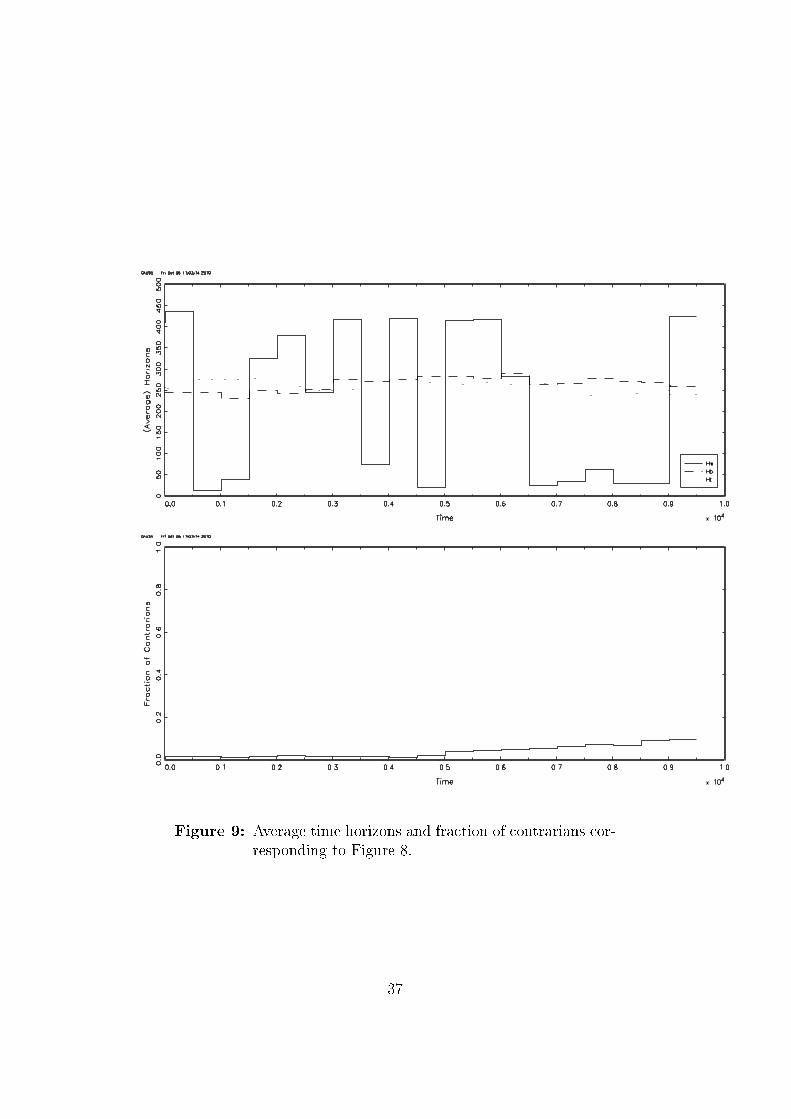
Figure 9: Average time horizons and fraction of contrarians cor-responding to Figure 8.

37

Figure 10: Example price and return series with correspondingvolatility (H observations). θ = 0.30, GA on.

38

Figure 11: Average time horizons and fraction of contrarianscorresponding to Figure 10.

39

Figure 12: Example price and return series with correspondingvolatility (H observations). θ = 0.40, GA on withρ = 2.

40

Figure 13: Average time horizons and fraction of contrarianscorresponding to Figure 12.

41

Figure 14: Simulation results. GA o�. Top left: Volatility ofreturns (over H). Top right: Di�erence in wealthbetween informed and noise traders. Center left:Transaction volume. Center right: Bid-ask spread.Bottom left: Market depth, de�ned as total amountof bid and ask orders in the LOB. Bottom right: Taxrevenues.

42

Figure 15: Simulation results. GA on. Top left: Volatility ofreturns (over H). Top right: Time horizons. Cen-ter left: Transaction volume. Center right: Bid-askspread. Bottom left: Market depth, de�ned as totalamount of bid and ask orders in the LOB. Bottomright: Fraction of contrarians.

43

Figure 16: Simulation results. GA on, θ = 0.3. Top left:Volatility of returns (over H). Top right: Time hori-zons. Center left: Transaction volume. Center right:Bid-ask spread. Bottom left: Market depth, de�nedas total amount of bid and ask orders in the LOB.Bottom right: Fraction of contrarians.

44