The Dynamics of Investment Projects: Evidence from Peru · The Peruvian economy is a major...

DT. N°. 2017-006

Serie de Documentos de Trabajo Working Paper series

Junio 2017

Los puntos de vista expresados en este documento de trabajo corresponden a los de los autores y no

reflejan necesariamente la posición del Banco Central de Reserva del Perú.

The views expressed in this paper are those of the authors and do not reflect necessarily the position of the Central Reserve Bank of Peru

BANCO CENTRAL DE RESERVA DEL PERÚ

The Dynamics of Investment Projects: Evidence from Peru

Marco Vega* y Rocío Gondo**

* Banco Central de Reserva del Perú ** Bank for International Settlements

The Dynamics of Investment Projects: Evidencefrom Peru∗

Rocıo Gondo and Marco Vega

June 6, 2017

Abstract

We analyse the effect of commodity price cycles on firm investment deci-sions at the project level, by considering the decision to delay, cancel orcomplete a project as initially announced. In particular, we use logit andduration models of competing risks on a novel dataset of announced in-vestment projects in Peru from different economic sectors. The empiricalframework for the timing of investment is motivated by real option modelsfor projects that take time to build, with commodity prices used as a proxyof expected future income and their volatility as a proxy for uncertainty.

Our results suggest that both a reduction in commodity prices and anincrease in volatility increase the probability to delay investment in themining sector, with an amplification effect when both simultaneously oc-cur. In other sectors, delays in implementation occur more often in periodsof high volatility. Probability regressions under a competing risk frame-work suggest that higher commodity prices lead to a higher probability ofcompletion in all sectors of the economy.

JEL Classification: E43, E51, E52Key words: Investment projects, panel logit, Competing Risks.

∗Revised version of the paper prepared for the closing conference of the BIS Consultative Councilof the Americas research network on ”The commodity cycle: macroeconomic and financial stabilityimplications”. We wish to thank participants in the research network for useful comments and sugges-tions. We also thank Paola Villa and Marcia Murillo for assistance. The views expressed in this paperare those of the authors and do not necessarily represent those of the Central Reserve Bank of Peru. Allremaining errors are ours.Rocıo Gondo: Bank for International Settlements and Central Reserve Bank of Peru ([email protected]). Marco Vega: Central Reserve Bank of Peru and Pontificia Universidad Catolicadel Peru ([email protected]).

1

mailto:[email protected]



1 Introduction

Large commodity price fluctuations in the recent decade have led policymakers to fo-

cus on the macroeconomic effects of these price swings in major commodity exporting

economies. This becomes especially relevant in times of falling commodity prices and

tightening of financial conditions in advanced economies, where external factors play

an important role in affecting variables such as investment, output and inflation in the

short run.

Even though some countercyclical policies were implemented to cope in the short

run, concern about long-term growth remains, given the tight link between commod-

ity prices and aggregate investment. A key channel is through the effect of uncertainty,

where commodity prices affect expected returns and risk of an investment project

outcome. For instance, higher commodity prices triggered an investment cycle in con-

struction and infrastructure (see Chapter 3, BIS (2016)). A persistent drop in invest-

ment reduces capital formation and thus potential output.

Real options models provide a theoretical framework for linking the timing of in-

vestment with uncertainty in expected future income streams. The standard model

predicts that higher uncertainty reduces incentives to invest. However, these result

is weakened/reversed under the following features: i) time to build with large fixed

scale projects, where the opportunity cost of delay increases with uncertainty, as a firm

cannot benefit if the news are good when projects are delayed (see Bar-Ilan & Strange

(1996)), and/or ii) financial constraints, where higher external financing costs provide

incentives to hurdle investment in the startup phase and use internal cash flows to

finance new investments at a later stage (see Bolton et al (2014)).

We motivate our empirical exercises with this framework. In particular, we use

commodity prices as a proxy variable of expected future income, and quantify their

effect on the timing of firm investment decisions at the project level. We explore the

2

evolution of investment projects and the decision of the firm to delay, cancel or com-

plete the project as initially announced by using a novel dataset of more than 1109

announced investment projects in Peru from different economic sectors between 2009

and 2015.

We provide a quantification of the effects of the qualitative results predicted by

real options models using this data. One key result is that we find a reversed effect

of uncertainty in the mining sector, in line with the modified real options model by

Bar-Ilan & Strange (1996), where a 1% increase in commodity price volatility in good

times leads to a 0.55 pp reduction in probability of delay, whereas in bad times this

effect falls by 0.36 pp.

We calculate the effect of commodity prices on the timing of investment, by using

logit models for the probability of delay, completion and cancellation. In particular,

for the mining sector, commodity prices are used as a proxy for expected future in-

come in the real options model. In other sectors, higher wealth in the mining sector

could spillover and increase expected profitability. Commodity price volatility enters

as a proxy of uncertainty and we test its link to the timing of investment. We also

consider the fact that, firms could decide to postpone the date of termination and/or

the beginning of production/ operations.

Some key results from our analysis are listed below:

1. Revising the decision to invest is affected by both commodity price growth rates

(linked to expected future income) and volatility (uncertainty), with differenti-

ated effects when prices are high or low. A decrease in commodity prices and

higher volatility in bad times leads to an increase in the probability for a project

to be unconfirmed.

As for magnitudes, a 10% increase in commodity prices leads to a 2.1 pp reduc-

tion in the probability of revision, with a slightly larger impact of 2.3 pp in the

3

sample of mining sector projects.

2. Once an investment project implementation is ongoing, the timing of investment

(given by delays during the startup phase) is also affected by the evolution of

commodity prices.

• Higher commodity prices increase expected profitability, either through its

effect on revenues (mining) or through spillovers from an income/wealth

effect. A 1% increase in commodity prices decreases the probability of delay

in the mining sector by 0.2 pp.

• We find evidence of the standard result for uncertainty in real options model,

where a 1% increase in volatility increases the delay probability by 0.18 pp

in all sectors except for mining. For the mining sector, we find a reversed

effect of uncertainty, in line with modified real options model with time

to build, where a 1% increase in volatility in good times reduces the delay

probability by 0.55 pp, compared to 0.36 pp lower effect in bad times.

3. Commodity prices do have a negative strong and statistically significant effect

on the probability of project completion in all sectors. Particularly in the mining

sector.

Related Literature. Our work relates to the analysis of investment decisions under

uncertainty. In particular, one strand of the literature that considers this link from

a theoretical perspective is the set of models for investment that use a real options

approach. Dixit & Pindyck (1994) lay the theoretical framework of a real options

model, where the cost of investing varies with time and there are limited investment

options in terms of expanding the current production capacity, which create put and

call options whose values affect the decisions to invest. These models link the timing of

investment to uncertainty about expected future income streams. A very well known

4

result from the standard real options model is that uncertainty delays the timing to

invest.

However, the link between uncertainty and timing to invest might be weakened

or overturned when considering some particular features. For instance, Bar-Ilan &

Strange (1996) find that, for large fixed scale projects that take time to build, uncer-

tainty not only increases the benefit of waiting to get more information about future

income, but also increases the opportunity cost of delay, given that the firm cannot

benefit from higher income if the news are good. Another feature that reverses this

result is the presence of financial and liquidity constraints, where Bolton et al (2014)

show that the wedge between external and internal financing costs provide incentives

to speed investment during the start up phase to generate internal cash flows. Our

empirical work is motivated by this theoretical framework, where we use commodity

prices as a proxy of expected future income streams, and we consider their effect on

timing of investment and uncertainty for projects that take time to build.

There is also a group of papers that focus on the empirical counterpart of real

options models. In particular, our work is related to the empirical applications that

consider large investment projects that take time to build. For instance, Bromander

& Atland (2012) analyse the effect of uncertainty in the case of sequential investment

with time to build, using a dataset of electrical power plants in the US. Similarly,

Kaldahl & Ingebrigtsen (2014) analyse this effect using a sample of gas power plants,

whereas Marmer & Slade (2015) apply the model to calculate the correlation between

uncertainty and investment in a sector with irreversible time to build features, using

data from the US copper mining sector. Our work considers a more diverse set of in-

vestment projects, by expanding the sample to different sectors of the economy, where

we evaluate the extent of spillover and uncertainty effects from changes in prices in

the mining sector to investment decisions in a variety of sectors.

5

The duration analysis for cancellation and completion of investment is closely re-

lated to Favero et al. (1994). They test the theoretical implications of a model of op-

timal investment timing and extraction rates for irreversible investment under un-

certainty by using a sample of oil fields in the United Kingdom. We apply a similar

methodology to our dataset of investment projects in different sectors, in particular,

to obtain the effects of timing of completion and cancellation.

Finally, another strand of the literature that relates to our work is the link between

terms of trade, investment and economic growth from a macroeconomic perspective

that focuses on aggregate data. We complement this by using more granular data

at the investment project level. For instance, Mendoza (1997) considers the negative

correlation between terms of trade variability and economic growth using a stochas-

tic endogenous growth model, whereas Basu & McLeod (1991) use an open economy

stochastic growth model to find that higher uncertainty in terms of trade fluctuations

lead to lower expected investment. Our results are consistent with the negative corre-

lation between investment decisions and commodity price volatility.

The paper is organised as follows. Section 2 presents a descriptive analysis of the

dataset of investment projects. Section 3 provides details on the empirical frameworks

used to analyse the timing and decisions to invest. Section 4 presents the results.

Section 5 concludes.

2 Descriptive analysis

The Peruvian economy is a major commodity exporter, especially in the mining sec-

tor, with metallic mining production accounting for 12 percent of GDP and mining

exports representing 55 percent of total exports1. As the revenues of this sector are

tightly linked to commodity prices, in particular to that of copper and gold, it is ex-

1This figure is calculated with data for 2015 and includes the refinement of mining products.

6

pected that not only ongoing production and export decisions are affected by com-

modity price movements, but also the decision to invest in new mining projects and

in expanding current investment units.

A first reason why we expect this link between commodity prices and investment

can be shown using information from the mining experts survey conducted by the

Central Bank of Peru. The survey shows that a drop in commodity prices is perceived

by mining sector experts as a very important cause of delays in new mining projects.

Figure 1 shows the results from the three most important causes of delays in new

mining projects, where 20 percent of experts consider commodity prices as one of the

key reasons.

Source: Mining experts survey. Central Bank of Peru.

Figure 1. Main causes of delay in new mining projects (in percent)

In order to analyze this effect, we use a novel dataset of investment project an-

nouncements that was compiled by the Central Reserve Bank of Peru (BCRP). It con-

siders 1109 announced projects from 2009 to October 2015. The information is ob-

tained from media and public press releases from private firms and from surveys and

interviews conducted by the BCRP. It covers investment projects in different sectors of

7

the economy: mining, hydrocarbons, electricity, industrial, agroindustry, telecommu-

nications and others. At each moment in time, each project is in either of four possible

states: confirmed, unconfirmed, canceled and completed. We define each category as

follows:

a. Confirmed projects. They have been granted permission and are about to be-

gin implementation. This process of implementation may take some time, even

years in some cases, especially for large investment projects in mining, hydro-

carbons, electricity or infrastructure sectors. Once confirmed, the investor may

decide to continue with its confirmed status or to revise or cancel the project.

The project will change status to completed once the investor confirms the be-

ginning of operations.

b. Unconfirmed projects. They are being considered by investors but have not be-

gan implementation or have stopped the implementation process. This state

is highly linked to regulatory issues and permit requirements required for in-

vestors to begin implementation. A confirmed project might switch to uncon-

firmed when tighter regulatory conditions are required to be fulfilled. As shown

later, very few unconfirmed projects switch back to confirmed after this.

c. Canceled projects. Investors have publicly announced that they will not con-

tinue implementation. Once canceled, the project is no longer implemented

again in the sample period.

d. Completed projects. The implementation process is completed and has began

operations.

It is clear that canceled and completed are absorbing states, whereas confirmed, re-

vised and unconfirmed states may switch to each other or to one of the absorbing

states. As shown in Figure 2, the amount of investment projects in the mining sector

8

has been increasing during the period of high commodity prices, whereas it shows a

slight drop in the last two years of the sample. This result partly considers the com-

pletion of some large investment projects such as Las Bambas (copper project), but

also the change to unconfirmed status as well as the lack of new investment projects

starting implementation.

Source: Central Bank of Peru.

Figure 2. Confirmed investment projects in the mining sector (in million of USD)

We present a summary table of descriptive statistics for the variables used in our

analysis in Table 1.

It is also important to note that besides the large drop in aggregate investment in

the last two years2, there has also been a shift in its composition. Figure 3 shows that

even though investment projects in the mining sector have contracted, the contraction

in confirmed investment projects in other sectors has not been quite as large. This

evidence suggests that there has been some reallocation of investment from sectors

directly linked to commodity exports to other sectors in the economy.

Tables 2 and Table 3 show the transition of investment projects between possible

states for two different periods: 2012, when commodity prices were relatively high

and started the downward trend, and 2015, which is the last available data. What we2Aggregate private investment in Peru fell 2.1 and 4.4 percent in 2014 and 2015, repectively.

9

I. All ProjectsVariable Units Mean Std. Dev. Skewness KurtosisTotal financing (size) Million of soles 366.9532 775.2048 3.9975 19.2011Foreign investment Million of soles 287.2809 721.2834 4.1344 20.8327Confirmed projects Dummy .6330 .4822 -.5526 -1.6976Unconfirmed projects Dummy .3517 .4777 .6221 -1.6159II. Projects with time to buildVariable Units Mean Std. Dev. Skewness KurtosisDelayed projects Dummy .3257 .5097 1.0494 4.0731Total financing (size) Million of soles 442.281 916.7544 4.4502 27.1267Commodity price growth Yoy var .4730 3.2403 4.1214 45.0348Historical volatility Std dev 2.0511 1.1921 .1655 6.5813Foreign investment Million of soles 38031.99 84280.13 4.6035 28.9870Confirmed projects Dummy .3572 .4792 .6374 1.4063Unconfirmed projects Dummy .1631 .3695 2.0687 5.2794Mining related social conflicts Number of conflicts 99.1429 11.2382 .5592 1.9392Total social conflicts Number of conflicts 279.6883 17.1970 -.3449 1.9308Time of delay Months .3809 3.5989 -77.2773 6136.921Conditional volatility Std dev .02307 .0085 1.3359 5.0371Number of projects 1109Number of periods 77

Table 1. Descriptive statistics

Source: Central Bank of Peru.

Figure 3. Confirmed investment projects in the mining sector (as percentage of confirmed projectsin all sectors)

observe is that the percentage of confirmed investment projects has declined, with a

higher participation of unconfirmed and canceled projects. However, by looking at

Table 2, we find some evidence that once commodity prices started declining, there

was a change in the composition of investment strategies, with a higher concentration

10

Initial state TransitionConfirmed Unconfirmed Canceled Completed

Confirmed 56.1 0.9 1.3 5.4Unconfirmed 0.4 18.4 0.4 0.4Canceled 0.0 0.0 4.9 0.0Completed 0.0 0.0 0.0 11.7

Table 2. Transition between states: 2012

Initial state TransitionConfirmed Unconfirmed Canceled Completed

Confirmed 44.5 0.0 0.6 0.9Unconfirmed 0.0 23.2 0.0 0.0Canceled 0.0 0.0 5.5 0.0Completed 0.0 0.0 0.0 25.3

Table 3. Transition between states: 2015

of projects that were transiting to a different state, besides the ones that were com-

pleted. This transition happened in both directions: considering as good news those

projects that were unconfirmed and became confirmed, but also considering as bad

news those which were confirmed and became unconfirmed or canceled.

In the case of confirmed projects, we also separate between the projects that suffer

delays from the projects that are being implemented according to the original sched-

ule. We track the particular months in which a firm announces a change in the com-

pletion period of the project.3 We use this subsample of confirmed projects only to

analyze the determinants of delays in investment projects. For reference, we show the

evolution of delayed projects in total confirmed projects in Figure 4.

In order to analyze the determinants of the decisions to delay an ongoing invest-

ment project, first we consider qualitative information from surveys to obtain some

possible determinants. As shown in Figure 1 from the Survey of Mining Experts, the

four main sources of delays are (i) operating delays, (ii) higher than expected costs, (iii)

3In order to build the dummy variable for the delayed state, we will later consider different defini-tions.

11

Figure 4. Delayed projects (as percentage of confirmed projects)

social conflicts and (iv) lower commodity prices. Given data availability limitations on

cost structures by each firm, we further explore the evolution of social conflicts and

commodity prices.

In the case of social conflicts, large investment projects are required to obtain sev-

eral permits related to environmental and social concerns. The approval of these per-

mits are tightly linked to the existence of social conflicts in the region, which either

delay or create uncertainty on whether the investment project can be implemented to

termination and whether the production process can take place. Figure 5 shows the

number of total social and environmental conflicts in all regions of Peru during the

sample period. It shows an upward trend in environmental conflicts, which in many

cases are related to either ongoing or future projects related to the mining sector.

With regards to commodity prices, media and press releases show some prelim-

inary evidence that mining companies have reduced production and delayed invest-

ment in new projects due to low commodity prices. As an example, this news from

October 2015: “Glencore plans to reduce the production of zinc and suspend opera-

tions in Peru: The main reason for the reduction is to preserve the value of Glencore’s

reserves in the ground at a time of low zinc and lead prices, which do not correctly

12

Source: Peruvian Ombudsman.

Figure 5. Number of social conflicts in Peru

value the scarce nature of our resources, the company said in a statement”.4

3 Framework

Simple framework: We start with the analysis of the proportion of confirmed projects

to total projects in the mining sector in terms of possible covariates suggested by the

description made in the previous section. We consider monthly data from 2009.5 to

2015.10 and run regressions of the form:

yt = α0 +α1yt−1 +α2Xt (1)

where the dependent variable yt is the proportion of confirmed mining projects to

total mining projects and Xt is a vector of covariates at time t. We want to measure

two types of covariates. First, covariates related to commodity price fluctuations such

as terms of trade, export prices, copper price or the margin between the copper price

and copper production cash costs. Second, variables related to social conflicts such as

total social conflicts in the country, conflicts related to environmental issues in general

4See Crispin & Grippa (2015) for more examples of these.

13

and the ratio of environmental to total social conflicts. This regression will provide

a first view of the relationship between investment projects and commodity prices as

well as the level of social conflictiveness. The drawback of the approach is that we do

not account for the changes in states that occur every month. It may be possible that

a reduction in commodity prices or an increasing level of social conflictivity or both

induce some confirmed projects to be revised, canceled or unconfirmed and therefore

explain the reduction in the ratio. But it also may be possible that the reduction in the

ratio is due to confirmed projects being completed. Thus, this exercise only provides

a partial and incomplete picture of confirmation dynamics.

Logit regression: Another aspect of the analysis concerns the decision to delay invest-

ment decisions. In order to do this, we use a panel logit regression with fixed effects

where the dependent variable, delayit, refers to whether project i has been announced

to delay its beginning of operations in time t. It takes a value of 1 if it has been an-

nounced to be delayed in the last 12 months and 0 otherwise. The estimated equation

takes the following form:

delayit = α0i +α1growthit +α2volatit +α3Xit (2)

Among the determinants, we consider two variables related to commodity price

fluctuations: the year on year percentage change (growthit) and the standard devia-

tion of the last 12 months (volatit) as a measure of volatility. In the case of mining

projects, we consider the price of the main commodity to be extracted from each min-

ing unit (i.e. copper, gold, silver and zinc) and for polymetallic or projects where the

main mineral is not identified, we use the terms of trade index. For other sectors, we

consider the terms of trade index as the commodity price for all projects.

Xit corresponds to a set of control variables, which include:

• conf lictit is the number of social conflicts. In the case of mining projects, we

14

consider the geographical location of each project, and use the number of so-

cial conflicts by region. For other sectors of the economy, we just consider the

aggregate nationwide number of social conflicts.

• f inancit is the amount of financial funding for the investment project and in-

cludes investment for all the duration of the implementation process, both the

amount that has already been disbursed as well as what is expected to be re-

quired to complete the project. This variable is a proxy of the size of the invest-

ment project.

• f diit is the amount of funding that comes from foreign investors and which is

categorized as foreign direct investment in the balance of payments accounts.

• volatnit is the volatility of commodity prices in periods of a downward trend in

these prices. We add this as an extra variable to analyze if there is a differentiated

effect due to uncertainty vs the willingness to speed up investment to reap on the

benefits in good times.

Competing risks framework: The dataset resembles duration data, we track each

project since the moment the confirmed status runs, the implementation of the con-

firmed project goes on until either of two terminal events or risks occur: (i) projects

are completed and therefore ready to be put in operation or (ii) projects are canceled.

In the dataset, some projects do not show either of these two terminal events because

there is right censoring. We may only see those events if we extend the data to the

future.

The implementation stage has a clear starting point, the month where it first ap-

pears in the data. It appears usually with the status of confirmed or unconfirmed.

Within this implementation period confirmed/unconfirmed projects may switch to a

revision status or switch to unconfirmed/confirmed status. In this first exercise we

15

treat all this implementation period as one state. Just as the diverse symptoms a pa-

tient that just arrives at the hospital has during the course of the treatment. In this

hospital example, the two terminal risks usually analyzed are the time of discharge

from the hospital and the time of death.

Therefore, just like survival or duration analysis we can study the probabilities

of duration until failure time but in this case, there are two competing causes that

explains when a project ceases to be a project. The two workhorses in competing risk

analysis are the cumulative incidence functions (CIFs) and competing risk regressions.

These two objects resemble the estimation of survival functions and the Cox propor-

tional hazard model in standard survival analysis.

The cause-specific cumulative incidence function (CIF), also known as sub-distribution

function is defined for example in Lawless (2011). Let T be the project duration time

until failure and let j be a cause of failure, the the CIF due to cause J = j is

Fj(t) = P r(T ≤ t, J = j) =

t∫0

λj(u)S(u)du (3)

where S(t) = P r(T ≥ t) = exp(−Λ(t)), with Λ(t) =2∑j

∫ t0λj(t). In this last expression λj(t)

are the cause-specific hazard ratio defined as

λj(t) = lim4t→0

P r[t ≤ T < t +4t, J = j | T ≥ t]4t

(4)

This is an instant probability of failure due to cause j conditional the project is

ongoing up to time t. The CIF represents the expected proportion of projects expe-

riencing a certain competing event over the course of time. In other words, it is the

probability of failure from cause j until time t in the presence of all other possible

causes. It depends on the cause-specific hazards for all other causes.

16

To see the effects of covariates, we put attention to two objects; cause-specific haz-

ard modeling or sub-distribution modeling. The proportional cause-specific hazard

model with covariates takes the form

λk(t | x,βk) = λ0(t) · gk(x,βk), k = 1,2, βk ∈Rpk (5)

where gk : Rp ×Rpk 7→ [0,∞], with gk(1,0) = 0 for all x

And the sub-distribution hazard modeling starts with the definition of the CIF for

cause j given covariates x

Fj(t | x) = P (T ≤ t, J = j | x) (6)

The analysis is done via the sub-distribution hazard function, so that

Fj(t | x) = 1− exp

−t∫

0

λj(s | x)ds

(7)

Fine & Gracy (1999) assumes the Cox regression of the form

Fj(t | x) = 1− exp(−Γj(t)exp(xβk)

)(8)

In sum, we are interested in estimating the shape of non-parametric CIFs as in

equation 3 and sub-distribution hazard regression as in 8.

4 Results

4.1 Confirmed investment projects

We start the analysis by getting a first grasp of how fluctuations in commodity prices

have directly affected the decision of firms in the mining sector to go ahead and imple-

17

ment their long-term investment decisions. For this, we consider the evolution of the

aggregate participation of investment projects across time, and its relationship with

commodity prices by sector. Table 4 presents the results of a regression considering

the participation of confirmed projects in the dataset of investment projects in the

mining sector as described in equation 1.

Dependent variable:

y=proportion of confirmed mining projects

(1) (2) (3) (4) (5) (6)

lag y 0.894∗∗∗ 0.894∗∗∗ 0.886∗∗∗ 0.872∗∗∗ 0.884∗∗∗ 0.884∗∗∗

(0.054) (0.067) (0.059) (0.058) (0.069) (0.069)

Conflicts −0.032 −0.005(0.042) (0.041)

Env. conflicts 0.009 −0.017 −0.017(0.066) (0.054) (0.054)

Conflict ratio 0.032(0.061)

Margin 0.012∗ 0.011 0.013∗

(0.006) (0.008) (0.007)

Log terms of trade 0.095∗ 0.087 0.087(0.051) (0.058) (0.058)

Constant 0.212 −0.002 0.024 −0.328 −0.243 −0.243(0.234) (0.314) (0.046) (0.331) (0.430) (0.430)

Observations 77 77 77 77 77 77R2 0.811 0.809 0.810 0.810 0.810 0.810Adjusted R2 0.803 0.801 0.802 0.802 0.802 0.802Residual Std. Error (df = 73) 0.032 0.032 0.032 0.032 0.032 0.032F Statistic (df = 3; 73) 104.148∗∗∗ 103.203∗∗∗ 103.655∗∗∗ 103.514∗∗∗ 103.661∗∗∗ 103.661∗∗∗

Note: ∗p<0.1; ∗∗p<0.05; ∗∗∗p<0.01

Table 4. The effects of commodity prices over the proportion of confirmed mining projects

Among the regressors in Xt in equation 1 we consider three alternative social con-

flict variables: the total amount amount of social conflicts, the total amount of envi-

ronmental conflicts and the ratio of environmental conflicts to total conflicts. We also

consider two alternative variables that proxy the evolution of commodity prices. The

first is the variable margin, this variable is constructed as the difference of the copper

price against its average cash cost in Peru. The second is the log of the Peruvian terms

18

of trade. A fall in copper prices is associated to a reduction of both, the price margin

and the terms of trade.

The results show that reduction in copper prices or a fall in the terms of trade

appears to have a negative effect in confirmed mining investment projects. These

effect tend to be significant in three out of the six specifications presented in table

4. In addition, social conflictivity affects the proportion of confirmed projects but

their impact in these regressions is not significant. The sign of the social conflict effect

over confirmed projects is negative suggesting that a rise in the level of social conflicts

reduce the proportion of confirmed projects.

This exercise is a first exploration suggesting the importance of commodity price

movements and social conflictivity on the decision of firms to confirm the execution of

the investment project. However, as we will see later, the reasons behind the transition

of a confirmed project to a terminal project, either to a completion or cancelation state

is important.

In addition, we implement a more granular analysis of the data, by exploring

the impact of commodity prices on the decisions of confirm/revise each investment

project separately. For this analysis, we also consider projects in different sectors of

the economy, and separate it between mining projects, which are more closely linked

to commodity prices, and other sectors of the economy, which might indirectly receive

spillover effects.

Basically, we consider two variables that account for the effect of commodity prices

on this decision, the variation and the volatility. When considering the mining sector,

we consider the price of the mining product that would be extracted at that particular

project. In other cases, we consider the terms of trade index. For the measure of

commodity price volatility, we consider two indicators: historical volatility, based on

the standard deviation of the past 12 months, and conditional volatility, obtained by

19

estimating a garch model5. The results are shown in Table 5.

Prob (uncofirmed)Historic volatility Conditional volatility

Mining Other All sectors Mining Other All sectorsMarginal effectsComm price growth −0.0023? −5.8e − 5? −0.0021? −0.0149? -0.0860 -0.0016Comm price volatility −0.0499? −8.3e − 5? −0.0062? −0.1044? −6.8e − 5? −0.0018?

Social conflicts(total) 0.0011? 4.0e − 6? 0.0002? 0.0013? 0.0001? 0.0015?

Foreign ownership −2.2e − 6? −2.0e − 8? −1.6e − 6? −5.9e − 6? −1.4e − 6? −2.0e − 5?

Total financing (size) 0.0003? 2.8e − 6? 0.0002? 0.0007? 0.0002? 0.0024?

LRchi2 465.02 3196.63 2903.57 418.18 3211.44 3021.06Obs 3080 7854 10934 3080 7854 10934Projects 40 102 142 40 102 142? denotes that the coefficient is statistically significant at the 5 percent level.

Table 5. Marginal effects on the probability of unconfirmed projects in all sectors of the economy.

If we consider all sectors in our estimation, we find that a fall in commodity prices

and lower commodity price volatility increase the probability of unconfirmed projects.

Higher prices lead to an increase in expected revenues and profitability of mining in-

vestment projects and create a positive spillover effect on other sectors of the economy

through an income effect. The results on volatility must be considered jointly with its

effect on the decision to delay. Higher uncertainty seem to be more related to larger in-

centives to delay a project rather than cancel or revise the decision to invest. Another

interesting feature is that social conflictivity increases the probability of revising or

unconfirming an investment project, which was captured by the results from the min-

ing expert survey. These results are robust to changes in the indicator of commodity

price volatility.

When we separate the sample between investment projects in the mining sector

and other sectors of the economy, as shown in Table 5, we observe that commodity

price variations and volatility have larger impacts on the probability of being uncon-

5We use the garch specification that provides the best fit, which in our case is given by garch(2,3) forthe price of copper and garch(2,2) for the price of gold.

20

firmed in the mining sector, as their profitability is more directly affected by commod-

ity prices.

4.2 Delayed investment projects

Another aspect of the investment decision, especially relevant in projects that take

time to build, is whether it is implemented on time. Therefore, we present the results

for the determinants of delays in investment projects by sector in Table 6.

Commodity prices have a significant impact on the decision to delay an invest-

ment project, both in terms of variations and volatility. On one hand, an increase in

commodity prices lead to a lower probability of delay, because the commodity price

in the case of the mining sector directly affects the future profitability of the project.

Higher commodity prices increase revenues when operations begin and minerals are

exported, so there is an extra incentive for firms to speed up investment and benefit

from a cycle of high commodity prices. In particular, an increase in commodity prices

by 1 percent in the last 12 months reduces the probability of delay in the mining sector

by 0.2 percent, compared to a non insignificant effect on other sectors of the economy,

when considering conditional volatility measures for uncertainty.

On the other hand, the effect of higher uncertainty of commodity prices depends

on whether prices are on an upward or downward trend. Related literature mentions

two effects of uncertainty. First, higher uncertainty create incentives for investors to

wait and obtain more information before making the decision to invest, as if they

have a valuable call option that is lost once the irreversible investment decision is

made. However, for investment projects that take time to build and funds must be

committed up front, investors also have a put option on the flexibility of the time of

completion, which create incentives to speed up investment.6 Our results show that

6See Bar-Ilan & Strange (1996). In that model the intuition is that the opportunity cost of delays

21

Historic volatility Conditional volatilityProb (delay) Mining Other All sectors Mining Other All sectorsMarginal effectsComm price growth −0.0022? −0.0069? −0.0176? −0.0017? 0.0208 −0.0135?

Comm price volatility −0.0055? 0.0018? 0.0016 −0.0075? −0.0011? −0.0011?

Volatility (downward) 0.0036? −0.0089 0.0051 0.0062? 0.0001 0.0003?

Social conflicts(total) 0.0002? −0.0016? 0.0007? 0.0002? −0.0001 0.0014?

Foreign ownership 1.6e − 7? 1.3e − 6 5.8e − 7? 2.1e − 7? −6.2e − 9 9.7e − 7Total financing (size) −1.7e − 5? 6.3e − 5 −3.6e − 5 −2.2e − 5? 5.2e − 5 −8.9e − 5

LRchi2 334.57 78.00 218.14 364.10 115.20 294.71Obs 2900 4285 7185 2900 4285 7185Projects 54 88 142 54 88 142? denotes that the coefficient is statistically significant at the 5 percent level, ?? at the 10 percent level.

Table 6. Marginal effects: Probability of delay in investment projects in all sectors of the economy

the second effect of increasing incentives to invest dominates, as there is a lower prob-

ability of delay when volatility increases. However, the first effect of desincentivising

investment is relevant for periods where commodity prices are declining.

Quantitative results for variables related to commodity price volatility show that,

in times of increasing commodity price (good news), an increase in volatility by 1

percent reduces the probability of a delay in the mining sector by 0.6 percent, whereas

in times of bad news the reduction in the probability of delay falls to only 0.2 percent.

However, for other sectors of the economy, we only find that the higher uncertainty

effect of commodity price volatility increases the probability of delay.

Additional results from the control variables show that larger projects have lower

probability of delay. This might be related to the fact that these projects usually in-

volve large sums that are irreversible and can therefore be categorized as a sunk cost.

Once part of the investment has already been disbursed, firms would be less likely to

delay the beginning of operations as they would like to reap on the income from the

increase with uncertainty because if good news take place, then the firm cannot benefit from it if it hasnot started the investment process.

22

mineral extraction as soon as possible.

We also calculate the marginal effects by changing the variable related to social

conflicts, by considering only the ones directly related to the mining sector, given

that these are directly related to the sector. Results are robust in terms of the social

conflictivity variable as well as for the price volatility indicator. This is shown in Table

7.

Prob(delay) in the mining sector(1) (2) (3) (4)

Marginal effectsComm price growth −0.0022? −0.0138? −0.0017? −0.0098?

Historical price volatility −0.0055? −0.0469? - -Historical volatility (downward) 0.0036? 0.0466? - -Conditional price volatility - - −0.0075? −0.0040?

Conditional volatility (downward) - - 0.0062? 0.0062?

Social conflicts(total) 0.0002? - 0.0002? -Social conflicts(mining) - 0.032? - 0.0028?

Foreign ownership 1.6e − 7? 1.8e − 6? 2.1e − 7? 1.8e − 6?

Total financing (size) −1.7e − 5? −0.0002? −2.2e − 5? −0.0002?

LRchi2 334.57 312.42 364.10 342.57? denotes that the coefficient is statistically significant at the 5 percent level.

Table 7. Marginal effects: Probability of delay in investment projects in the mining sector

Now we focus our attention on mining projects only and analyse if there is a dif-

ferentiated impact of commodity prices on the revised completion dates when an in-

vestment project is delayed, and whether more abrupt commodity price fluctuations

lead to longer delay horizons7. For this, we constructed a dependent variable with the

number of months between the revised expected and original dates of completion.

Table 8 shows the results. A longer delay for the expected time of completion is ex-

pected following a reduction in commodity prices and an increase in commodity price

volatility, consistent with the effects on the probability that an investment project is

7We also analysed the delay period with respect to the original date of expected completion forprojects in other sectors but did not find evidence of different timings in the delays.

23

Mining sector: Announced delay (in number of months)Historic volatility Conditional volatility

(1) (2) (3) (4) (5)Comm price growth −0.0285? −0.0076?? 0.0032 −0.0074? 0.0021Comm price volatility −0.0141 −0.0612? −0.0319? −0.0713? 0.0004Comm price volatility (downward) — 0.0683? 0.0324? 0.0944? 0.0006?

Foreign ownership 1.9e − 6 2.4e − 6? 2.8e − 6? 2.7e − 6? 2.9E − 6?

Total financing (size) −0.0003? −0.0001 −0.0002? −0.0003? −0.0025?

Conflict (total) 0.0030? 0.0025? - 0.0025? -Mining conflicts - - 0.0134? - 0.0130?

F-test 27.35 30.54 73.33 37.71 76.17R2 0.1020 0.0645 0.1162 0.0634 0.1202? denotes that the coefficient is statistically significant at the 5 percent level, ?? at the 10 percent level.

Table 8. Determinants of announced delays of investment in the mining sector.

delayed. Therefore, the two results show that a period of falling commodity prices

with sharp fluctuations not only increases the chance that the project takes more time

to be implemented but it will start its operations in a much longer period of time. Re-

garding other project specific determinants, we find that social conflictivity increases

the time of delay whereas larger projects tend to be implemented in a shorter period

of time.

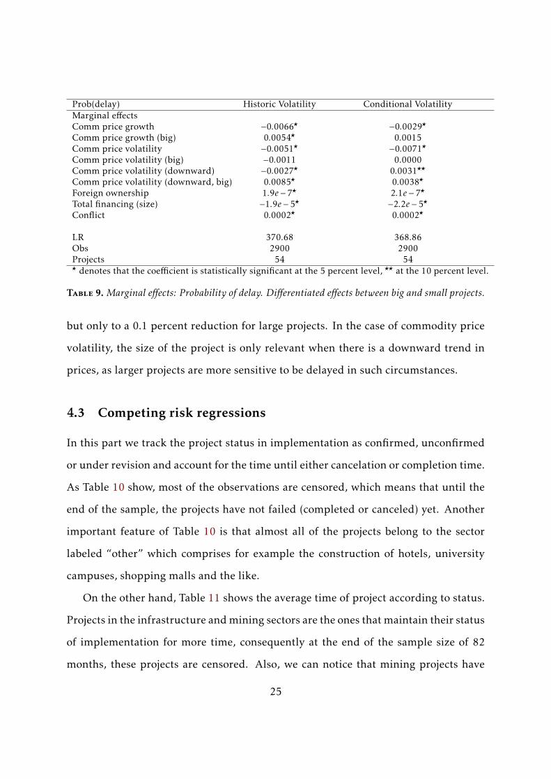
Another exercise that we considered is the existence of a differentiated effect be-

tween small and large investment projects. For this, we separated the projects in two

groups according to the size of total financing. We established the threshold at the

median of the distribution of projects in our database. We focused on the effect of

commodity price growth and volatility of small and large investment projects. Table

9 shows the results.

Results show the existence of differentiated effects for larger projects especially

in the mining sector. The probability of a large mining project being delayed is less

sensitive to commodity price fluctuations, where a one percent increase in commodity

prices leads to a 0.6 percent lower probability of being delayed for small projects,

24

Prob(delay) Historic Volatility Conditional VolatilityMarginal effectsComm price growth −0.0066? −0.0029?

Comm price growth (big) 0.0054? 0.0015Comm price volatility −0.0051? −0.0071?

Comm price volatility (big) −0.0011 0.0000Comm price volatility (downward) −0.0027? 0.0031??

Comm price volatility (downward, big) 0.0085? 0.0038?

Foreign ownership 1.9e − 7? 2.1e − 7?

Total financing (size) −1.9e − 5? −2.2e − 5?

Conflict 0.0002? 0.0002?

LR 370.68 368.86Obs 2900 2900Projects 54 54? denotes that the coefficient is statistically significant at the 5 percent level, ?? at the 10 percent level.

Table 9. Marginal effects: Probability of delay. Differentiated effects between big and small projects.

but only to a 0.1 percent reduction for large projects. In the case of commodity price

volatility, the size of the project is only relevant when there is a downward trend in

prices, as larger projects are more sensitive to be delayed in such circumstances.

4.3 Competing risk regressions

In this part we track the project status in implementation as confirmed, unconfirmed

or under revision and account for the time until either cancelation or completion time.

As Table 10 show, most of the observations are censored, which means that until the

end of the sample, the projects have not failed (completed or canceled) yet. Another

important feature of Table 10 is that almost all of the projects belong to the sector

labeled “other” which comprises for example the construction of hotels, university

campuses, shopping malls and the like.

On the other hand, Table 11 shows the average time of project according to status.

Projects in the infrastructure and mining sectors are the ones that maintain their status

of implementation for more time, consequently at the end of the sample size of 82

months, these projects are censored. Also, we can notice that mining projects have

25

Sector Censored Canceled Completed

1 Agro-industry 40 0 32 Electricity 73 2 263 Hydrocarbon 54 1 154 Industry 88 2 185 Infrastructure 56 3 186 Mining 86 3 187 Other 483 2 758 Fishing 10 0 49 Telecom 27 0 2

Table 10. Number of projects according to status

been canceled earlier.

Sectors Censored Canceled Completed

Agro-industry 34.3 15.3Electricity 36.3 16.0 38.1Hydrocarbon 39.6 25.0 26.1Industry 34.8 20.0 25.7Infrastructure 43.7 7.0 25.9Mining 45.4 38.3 26.1Other 32.5 25.0 16.2Fishing 35.2 16.3Telecom 36.0 37.0

Table 11. Average time of projects according to status

Cumulative incidence functions: With this type of competing risk data by sectors,

we first estimate the CIFs by sector as shown in Figure 6. The figure shows that prob-

abilities of both competing risks according to project age in each sector. In all cases,

completion is more likely than cancelation. In general, the probability of project can-

celation is low, below ten percent and only in mining and infrastructure they rich to

about five percent. In the mining sector, the probability of cancelation smoothly in-

creases as project age grows. In the infrastructure sector, cancelation probability only

rises during the initial months.

26

Regarding completion probabilities, the mining sector probability only rises to

about 25 percent at the end of the sample. In general all completion probabilities

end up at about 30 percent except the electricity sector probabilities which end up in

about 60 percent after 82 months of project implementation. This feature is the result

of the huge amount of censoring in the data. It is not possible to know whether the

shape of the CIFs bend upwards in the next five years after the sample or if they will

keep their concave pattern.

Proportional sub-distribution hazard regressions: Now we perform the regression

described in equation 8. The results are shown in tables A-1 through A-10 in appendix

A. Given the small number of canceled observations, the results about cancelations

may not be robust. However, the results about duration of project until completion

are more meaningful.

In all regressions, we used three covariates for each project. First, a variable linked

to commodity price variations since the inception of the project until failure time.

In the case of censoring the change is from the project inception time to the final

observation. In all cases we use the logarithmic change in the general export price

index except for the mining sector where the change in margins is used. The second

covariate used is the size of foreign investment associated to the project at the time

of failure or censoring time. The third variable is the change in the environmental

conflict ratio from inception to failure or censoring.

The key result is that an fall in export prices or a fall in margins reduce the proba-

bility of completion in all sectors of the economy. This results is compatible with pre-

vious results presented in the paper and highlight the important role of export prices

to speed up projects, even if the particular investment project is not directly related

to the commodity sector. The fall in the completion probability may be due to delays

associated with the reduction of profitability as shown in the previous subsection.

27

Electricity Hydrocarbons

0 10 20 30 40 50 60 70

0.0

0.1

0.2

0.3

0.4

0.5

0.6

Months of project

Pro

babi

lity

canceledcompleted

0 20 40 60 800.

00.

10.

20.

30.

40.

50.

6

Months of project

Pro

babi

lity

canceledcompleted

Industry Infrastructure

0 20 40 60 80

0.0

0.1

0.2

0.3

0.4

0.5

0.6

Months of project

Pro

babi

lity

canceledcompleted

0 20 40 60 80

0.0

0.1

0.2

0.3

0.4

0.5

0.6

Months of project

Pro

babi

lity

canceledcompleted

Mining Other

0 20 40 60 80

0.0

0.1

0.2

0.3

0.4

0.5

0.6

Months of project

Pro

babi

lity

canceledcompleted

0 20 40 60 80

0.0

0.1

0.2

0.3

0.4

0.5

0.6

Months of project

Pro

babi

lity

canceledcompleted

Figure 6. Cumulative incidence function by sector28

Also, an important result is that a rise in the proportion of environmental conflicts

reduce significantly the probabilities of completion in all sectors except electricity. A

rise in environmental conflicts may be linked to a rise in total costs associated to the

project that produces delays and hinders completion.

To further examine the effect of commodity prices on the two competing events in

the mining sector, we graph the predicted CIF curves under a benchmark case com-

pared to a counterfactual situation for the values of the covariates. In the benchmark

case, the covariates for the mining sector are the average levels. In the base case, for-

eign direct investment associated to the project is USD 527 millions, margins have

decreased in 26 percent and the conflicivity ratio has increased 21 percent. In the

counterfactual case we keep all based values but the margins. Specifically, margins do

not fall in the counterfactual case.

The results are shown in Figure 7. As observed, if margins had not fallen, the com-

pletion probabilities would have doubled towards the end of the fifth year from 20 to

40 percent. The same happens with the cancelation probabilities but the probabilities

are so small that statistically they might be the same.

5 Conclusions

This paper uses a novel dataset of investment project states at the project levels across

sectors in the Peruvian economy since 2009 to October 2015. A number of models

are run to uncover basic features and relationships with covariates. In particular the

paper is interested on the effect of commodity prices on investment projects in general

and mining investments in particular.

Commodity prices are highly relevant for investment project decisions by firms,

not only in sectors whose profitability is directly affected by them(ie mining sector in

29

Cancelation Completion

0 10 20 30 40 50 60

0.00

0.01

0.02

0.03

0.04

0.05

0.06

0.07

Months of project

Pro

babi

lity

basecounterfactual

0 10 20 30 40 50 60 70

0.0

0.1

0.2

0.3

0.4

0.5

Months of project

Pro

babi

lity

basecounterfactual

Figure 7. Predicted CIFs under base and counterfactual case

Peru), but also create spillover effects in other sectors of the economy as well. A de-

crease in commodity prices and higher commodity price volatility in bad times leads

to an increase in the probability for a project to be unconfirmed. Mining projects are

quantitatively more affected by commodity prices, as expected profitability in other

sectors come only through spillover effects.

In the case of delays of investment projects that are already being implemented,

this decision is also affected by the evolution of commodity prices, by both growth

rates and volatility. In the case of volatility, higher uncertainty increases incentives

to postpone projects for all sector of the economy. However, a second effect that is

relevant in the case of the mining sector is that the possibility of better news than

expected leads to higher incentives to start production and reap on the benefits of this

in terms of higher profits.

Once an investment project implementation is ongoing, the probability that a firm

chooses to delay its completion and start production is also affected by the evolution

of commodity prices. For the mining sector, both commodity price growth rates and

30

volatility matter, whereas the delay probability is only affected by volatility for other

sectors. An increase in commodity prices reduce incentives to delay by affecting the

expected profitability of the project. In the case of volatility, if taken as a measure of

uncertainty, higher volatility leads to more incentives to postpone or delay investment.

However, a second effect that is relevant in the case of the mining sector is that the

possibility of better news than expected leads to higher incentives to start production

and reap on the benefits of this in terms of higher profits.

Last but not least, commodity prices do have a negative strong and statistically

significant effect on the probability of project completion in all sectors. Particularly in

the mining sector.

Future avenues of research point to considering the transmission mechanisms that

generates the spillover effect to other sectors of the economy. In particular it would

be interesting to analyse the interaction between mean and volatility spillovers in the

context of multivariate volatility models, following the methodology proposed by Ser-

letis and Xu (2016, 2017). They find that VARMA, GARCH-in-Mean and BEKK models

confirm the presence of spillover effects using oil, gas and coal prices. An extension of

this to other types of metals that are the main commodity exports of other countries

in the region, such as copper, would be of particular interest.

Also, given that commodity price volatility generates higher uncertainty and in-

centives to delay or cancel an investment project, identifying the transmission chan-

nel would be key to target policy recommendations that could ameliorate the effect

of commodity price shocks on aggregate investment and its implications on long term

growth potential. One possible channel is through the existence of input output link-

ages between the mining sector and other sectors of the economy, as investment in new

mining units would, for instance, require complementary investment in infrastructure

and electricity.

31

References

Bank for International Settlements (2016). Annual Report.

Bar-Ilan, A., and Strange, W. C. (1996). Investment lags. The American Economic Re-

view, 86(3), 610-622.

Basu, P & D McLeod (1991). Terms of trade fluctuations and economic growth in

developing economies. Journal of Development Economics, Elsevier, vol. 37(1-2),

pages 89-110, November.

Bolton, P, N Wang, and J Yang (2014). Investment under uncertainty and the value of

real and financial flexibility. NBER Working Paper 20610.

Crispin Y. and F. Grippa (2015). Sector minero en el Peru, BBVA Re-

search. URL: https://www.bbvaresearch.com/wp-content/uploads/2015/11/

Sector-Minero-en-el-Peru.pdf

Bromander, G. and E. Atland (2012). An Empirical Study of Sequential Investments

with Time-To-Build. Department of Industrial Economics and Technology Manage-

ment, Norwegian University of Science and Technology

Dixit, A.K. and Pindyck, R.S. (1994). Investment under uncertainty. Princeton uni-

versity press.

Favero, C.A., Hashem Pesaran, M. and Sharma, S. (1994). A duration model of irre-

versible oil investment: theory and empirical evidence. Journal of Applied Economet-

rics, 9(S1), pp.S95-S112.

Fine, J. P., & Gray, R. J. (1999). A proportional hazards model for the sub-distribution

of a competing risk. Journal of the American statistical association, 94(446), 496-509.

32

https://www.bbvaresearch.com/wp-content/uploads/2015/11/Sector-Minero-en-el-Peru.pdf

https://www.bbvaresearch.com/wp-content/uploads/2015/11/Sector-Minero-en-el-Peru.pdf

Gray, B. (2013). cmprsk: Sub-distribution Analysis of Competing Risks. R package

version 2.2-2. URL: http://CRAN.R-project.org/package=cmprsk

Kaldahl, J.A. and Ingebrigtsen, K. (2014). Sequential investment in gas fired power

plants: A real options analysis.

Lawless, J. F. (2011). Statistical models and methods for lifetime data (Vol. 362). John

Wiley & Sons.

Marmer, V and ME Slade (2015) Investment and uncertainty with time to build: Evi-

dence from US copper mining. Mimeo.

Mendoza, E.G. (1997). Terms-of-trade uncertainty and economic growth. Journal of

Development Economics, 54(2), pp.323-356.

C. Sax and P. Steiner. tempdisagg: Methods for Temporal Disaggregation and In-

terpolation of Time Series, 2013. URL: http://CRAN.R-project.org/package=

tempdisagg. R package version 0.22. [p80]

Serletis, Apostolos and Libo Xu (2016). Volatility and a century of energy markets

dynamics. Energy Economics 55, 1-9.

Serletis, Apostolos and Libo Xu (2017). The zero lower bound and crude oil and finan-

cial markets spillovers. Macroeconomic Dynamics, forthcoming.

33

http://CRAN.R-project.org/package=cmprsk

http://CRAN.R-project.org/package=tempdisagg

http://CRAN.R-project.org/package=tempdisagg

Appendix

A Tables

coef exp(coef) se(coef) z p-valueForeign finance -0.81 0.45 0.06 -12.5 0Growth of export prices 0.67 1.95 0.03 25.0 0Growth of conflict ratio -8.15 0.00 0.46 -17.8 0

exp(coef) exp(-coef) 2.5% 97.5%Foreign finance 0.45 2.24 0.39 0.51Growth of export prices 1.95 0.51 1.85 2.06Growth of conflict ratio 0.00 3469.54 0.00 0.00

Table A-1. Electricity: Cancellation regression

coef exp(coef) se(coef) z p-valueForeign finance -0.00 0.10 0.00 -1.74 0.08Growth of export prices 0.03 1.03 0.01 2.88 0.00Growth of conflict ratio -0.02 0.99 0.02 -0.93 0.35


Table A-2. Electricity: Completion regression

34

coef exp(coef) se(coef) z p-valueForeign finance -0.00124 0.999 0.00106 -1.174 0.2400Growth of export prices -0.00778 0.992 0.04010 -0.194 0.8500Growth of conflict ratio -0.32661 0.721 0.10534 -3.101 0.0019


Table A-3. Hydrocarbons: Cancelation regression

coef exp(coef) se(coef) z p-valueForeign finance -0.000565 0.999 0.000294 -1.92 0.05500Growth of export prices 0.043446 1.044 0.011613 3.74 0.00018Growth of conflict ratio -0.096925 0.908 0.029413 -3.30 0.00098


Table A-4. Hydrocarbons: Completion regression

35

coef exp(coef) se(coef) z p-valueForeign finance -0.000865 0.999 0.00173 -0.501 6.2e-01Growth of export prices 0.036612 1.037 0.00887 4.126 3.7e-05Growth of conflict ratio -0.020403 0.980 0.04410 -0.463 6.4e-01


Table A-5. Industry: Cancelation regression

coef exp(coef) se(coef) z p-valueForeign finance -0.000756 0.999 0.000884 -0.856 3.9e-01Growth of export prices 0.030492 1.031 0.004457 6.842 7.8e-12Growth of conflict ratio -0.098769 0.906 0.033534 -2.945 3.2e-03


Table A-6. Industry: Completion regression

36

coef exp(coef) se(coef) z p-valueForeign finance 0.000193 1.000 0.00185 0.104 0.92000Growth of export prices 0.041986 1.043 0.01254 3.348 0.00081Growth of conflict ratio -0.081508 0.922 0.03061 -2.663 0.00770


Table A-7. Infrastructure: Cancelation regression

coef exp(coef) se(coef) z p-valueForeign finance 0.000831 1.001 0.000637 1.30 1.9e-01Growth of export prices 0.048407 1.050 0.008055 6.01 1.9e-09Growth of conflict ratio -0.056433 0.945 0.020004 -2.82 4.8e-03


Table A-8. Infrastructure: Completion regression

37

coef exp(coef) se(coef) z p-valueForeign finance -0.000441 1.000 0.000415 -1.062 0.29Margin 0.009080 1.009 0.012809 0.709 0.48Growth of conflict ratio -0.039287 0.961 0.030111 -1.305 0.19

exp(coef) exp(-coef) 2.5% 97.5%Foreign finance 1.000 1.000 0.999 1.00Margin 1.009 0.991 0.984 1.03Growth of conflict ratio 0.961 1.040 0.906 1.02

Table A-9. Mining: Cancelation regression

coef exp(coef) se(coef) z p-valueForeign finance 0.00 1.000 0.000312 0.139 8.9e-01Margin 0.03 1.031 0.006678 4.522 6.1e-06Growth of conflict ratio -0.07 0.933 0.020699 -3.343 8.3e-04

exp(coef) exp(-coef) 2.5% 97.5%Foreign finance 1.000 1.00 0.999 1.001Margin 1.031 0.97 1.017 1.044Growth of conflict ratio 0.933 1.07 0.896 0.972

Table A-10. Mining: Completion regression

38

B Graphs

agro−industry

Time

%

2009 2011 2013 2015

0.0

0.2

0.4

0.6

electricity

Time

%

2009 2011 2013 2015

0.5

0.6

0.7

0.8

hidrocarbons

Time

%

2009 2011 2013 2015

0.65

0.75

0.85

industrial

Time

%

2009 2011 2013 2015

0.6

0.7

0.8

0.9

1.0

infrastructure

Time

%

2009 2011 2013 2015

0.5

0.6

0.7

0.8

mining

Time

%

2009 2011 2013 2015

0.50

0.60

0.70

0.80

other

Time

%

2009 2011 2013 2015

0.5

0.6

0.7

0.8

0.9

1.0

fishing

Time

%

2009 2011 2013 2015

0.5

0.6

0.7

0.8

0.9

1.0

telecom

Time

%

2009 2011 2013 2015

0.5

0.7

0.9

Figure B-1. Proportion of confirmed projects to total projects in each sector

39

The Dynamics of Investment Projects: Evidence from Peru · The Peruvian economy is a major...

Documents

Transcript of The Dynamics of Investment Projects: Evidence from Peru · The Peruvian economy is a major...