The Dynamics of Ex-Ante High- Frequency Liquidity: An ... · with these liquidity measures is that...

The Dynamics of Ex-Ante High-Frequency Liquidity: An Empirical Analysis Georges Dionne Xiaozhou Zhou January 2016

CIRRELT-2016-02

The Dynamics of Ex-Ante High-Frequency Liquidity: An Empirical Analysis

Georges Dionne1,*, Xiaozhou Zhou1,2

1 Interuniversity Research Centre on Enterprise Networks, Logistics and Transportation (CIRRELT) and Department of Finance, HEC Montréal, 3000 Côte-Sainte-Catherine, Montréal, Canada H3T 2A7

2 Department of Finance, Université du Québec à Montréal, C.P. 8888, succ. Centre-ville, Montréal, Canada H3C 3P8

Abstract. Using tick-by-tick data and the reconstructed open LOB data from the Xetra trading system, we investigate the impact of trade duration, quote duration and other exogenous variables on ex-ante liquidity embedded in an open LOB. Our modeling involves decomposing the joint distribution of the ex-ante liquidity measure into simple and interpretable distributions. The decomposed factors are Activity, Direction and Size. Our results suggest that trade durations and quote durations do influence the exante liquidity changes. Short-run variables, such as spread change and volume, also predict the probability of liquidity changes.

Keywords. Decomposition model, limit order book, Xetra Liquidity Measure (XLM), ex-ante liquidity, LogACD process.

Acknowledgements: We thank Yann Bilodeau for his help in constructing the dataset and comments. We also thank Christian Gourieroux, Diego Amaya, Gabriel Yergeau, Maria Pacurar, Tolga Cenesizoglu for their remarks. Georges Dionne acknowledges financial support from the Social Sciences and Humanities Research Council (SSHRC) in Canada and the Canada Foundation for Innovation, and Xiaozhou Zhou thanks Fonds de recherche du Québec - Société et culture (FRQSC), the Canada Research Chair in Risk Management, and Centre interuniversitaire sur le risque, les politiques économiques et l’emploi (CIRPEE) for financial support.

Results and views expressed in this publication are the sole responsibility of the authors and do not necessarily reflect those of CIRRELT.

Les résultats et opinions contenus dans cette publication ne reflètent pas nécessairement la position du CIRRELT et n'engagent pas sa responsabilité. _____________________________

* Corresponding author: [email protected]

Dépôt légal – Bibliothèque et Archives nationales du Québec Bibliothèque et Archives Canada, 2016

© Dionne, Zhou and CIRRELT, 2016

1 Introduction

Liquidity is a complex concept and has been one of the most important issues in financial researchfor a long time. The term ’liquidity’ is interpreted differently by various market participants.Market regulators see liquidity as either the capacity to buy and sell a large quantity of financialsecurities, or as the total turnover of assets in a given time interval. For individual traders,the level of liquidity relates more to the quantity available when changing their positions atbuying or selling side. Nowadays, liquidity evolves with the development of high-frequencytrading (HFT) 1. As shown by Hendershott and Riordan (2013), for stocks of DAX30, high-frequency traders present 52% of market order volume and 64% of nonmarketable limit ordervolume. Understanding how liquidity behaves in this HFT environment is essential for all buy-side traders2 and market regulators. However, there are few quantitative analysis of the ex-anteliquidity in an ultra high frequency environment. The objective of this paper is twofold. First wemodel the dynamic of ex-ante liquidity, which is offered by the Limit Order Book (LOB), froma general view through the analysis of available electronic data in the Xetra open LOB system.Second, we investigate the effect of exogenous high-frequency variables on this ex-ante liquiditymeasure.

Ex-ante liquidity is embedded in LOB and there already exists a large number of theoretical mi-crostructure models emphasizing the state of LOB because of its importance in providing marketliquidity and discovering price formation. However, there is a huge gap between theoretical andempirical research for the analysis of high-frequency trading mechanism and liquidity. This isdue to the fact that market order traders and LOB traders behave in a complicated way, andtheoretical models do not capture all of these complexities. For example, the LOB traders inParlour (1998) cannot choose multiple limit-order price strategies; in Foucault (1999), the life-time of a limit order can not last more than one period; and in Foucault et al. (2005), the limitorders cannot be canceled once they are placed in the open LOB. All these restrictions may havean impact on the ex-ante liquidity provision.

In the market microstructure framework, other than spontaneous supply and demand in the mar-ket, the liquidity provision inherently depends on various exogenous factors such as the tradingmechanism, the information disclosure process and regulatory issues. For instance, Viswanathanand Wang (2002) show that the slope of the equilibrium bid price is flatter than that in adealership market since the discriminatory pricing rule intensifies the liquidity provision. Theempirical results of Boehmer et al. (2005) suggest that an increase in pre-trade transparencycan improve market liquidity. Riordan and Storkenmaier (2012) examine the effect of a techno-logical upgrade on the market liquidity of 98 actively traded German stocks and show that botheffective spreads and average price impacts drop with the upgrade. Bloomfield et al. (2015) use

1In high-frequency trading, traders make profit by using algorithms to quickly process information and detectthe trade opportunities.

2Buy-side traders includes invididuals, mutual funds, financial institutions, etc.

1


CIRRELT-2016-02

a laboratory market to investigate how the ability to hide orders affects market liquidity andtraders’ strategies and suggest that liquidity and informational efficiency are not affected whentraders adapt their behavior to the different opacity regimes. Another important concern is theavailability of data. In previous studies, widely used high-frequency liquidity measures, suchas trade impact and effective spread, are obtained from trade-related databases. One problemwith these liquidity measures is that they are measured only when there is a trade. With theintroduction of an open LOB trading mechanism, the access to more complete high-frequencydata becomes possible. As a result, we can use the information in the LOB to compute twodifferent measures of liquidity: ex-ante liquidity and ex-post liquidity. Up to now there existslittle consensus on the most appropriate liquidity measure in terms of efficiency and accuracydue to its multi-faceted complexity in both cross-sectional (depth, width, resiliency, etc.) andfrequency (high-frequency or low-frequency based) dimensions.

This empirical paper concentrates on the dynamic of the ex-ante liquidity embedded in an openLOB (depth and price impact) and the effect of high-frequency variables on its dynamics 3.Recent studies related to ex-ante liquidity include Irvine et al. (2000), Coppejans et al. (2004),Domowitz et al. (2005), Giot and Grammig (2006), Beltran-Lopez et al. (2009), and Beltran-Lopez et al. (2011). According to Aitken and Comerton-Forde (2003), ex-post liquidity measuresinvolve trade-based measures, while ex-ante liquidity measures are order-based. The formermeasures are the most widely used and indicate what the traders have obtained in the realizedtransaction. The second group captures the cost related to potential immediate trading. Thiscost is quasi-fixed for traders with a small quantity to trade and is equal to half of the bid-askspread. In this case we do not need any information about the LOB. However, for the largertraders, the spread will surely underestimate the associated cost when the quantity to tradeis larger than the quantity available at first level. This requires a liquidity measure that canallow for volume-related price impact. To this end, we construct and model the ex-ante liquiditymeasure with different trading volumes (from 5 000 to 2 5000 euros).

Another characteristic of the ex-ante liquidity measure is that it can be computed even whenthere is no trade. As noted by Beltran-Lopez et al. (2011), in 2004, for the average stock inthe DAX30 of Xetra trading system, the average daily number of limit orders is 12,785, i.e.25 limit orders per minute, whereas the average number of trades is four per minute. Thecorresponding numbers are 334 per minute for limit orders and 10 per minute for trades in July2010. As the trend of high frequency trading continues to increase rapidly, market regulators andinstitutional investors need more continuous measures of liquidity to update their informationset. The traditional ex-post liquidity measurement cannot meet this requirement. The temporalrelation between updates of LOB and transactions is shown in Figure 1 where transactions andupdates of LOB are denoted by circles and squares respectively. As we see the quote updates

3A large number of empirical studies examine the effect of HFT on the ex-post liquidity (Hendershott et al.(2011), Hasbrouck and Saar (2013), Menkveld (2013), Hendershott and Riordan (2013), Brogaard et al. (2014),among others). Survey articles include Biais and Wooley (2011), Johes (2012), O’Hara (2015).

2


CIRRELT-2016-02

are usually much more frequent than the trade updates and may then contain more informationon liquidity.

[Insert Figure 1 here]

This study models the evolution of ex-ante liquidity measurement using a decomposition modelwhich allows for various factors in a flexible way and investigates the effect of exogenous highfrequency variables on this ex-ante liquidity measurement. To our knowledge, we are the firstto consider modeling ex-ante liquidity using a decomposition model and including a large set offactors. Given the particularity of UHF data and the complexity of microstructure analysis, onepossible modeling framework involves consistently decomposing the joint distribution of a targetvariable into simple and interpretable distributions. The idea of decomposition was pioneeredby Rogers and Zane (1998) and aims at constructing observation-driven models in the senseof Cox et al.(1981). The decomposition model was first used in analyzing transaction pricedynamics. Hausman et al. (1992) and Russell and Engle (2005) propose an AutoregressiveConditional Multinomial (ACM) and ordered Probit model respectively. Rydberg and Shephard(2003) manage to achieve the same goals by decomposing the joint distribution of tick-by-ticktransaction price changes into three sequential components. The first component is designated’active’ and used to indicate whether the price change will occur. The second component called’direction’, indicates the direction of price change, and the third, ’size’, measures the absolute sizeof the price change.The decomposition model is used to predict price movements or price levelwith the help of simulations. McCulloch and Tsay (2001) aim at modeling the transaction pricechange process using the decomposition model. In their framework, they initialize a price changeand duration (PCD) model that decomposes the price changes into four factors and introducetime and liquidity dimension in modeling price change dynamics. The duration between twoconsecutive transactions and the number of trades during this duration are modeled as implicitfactors for the price changes. In total, they use six conditional models to capture the dynamicof price changes. Manganelli (2005) applies the decomposition methodology in investigating thesimultaneous interaction between duration, volume and return. Two subgroups, classified bythe trade intensity, perform different dynamics. The decomposition framework remains flexiblefor more complicated modeling and, depending on different modeling assumptions, addition ordeletion of certain factors is possible.

Our paper differs from the existing literature in several dimensions. First of all, instead of ag-gregating the time for a fixed interval, our analysis contains a time dimension. Specifically, ourpaper investigates the role of trade and quote durations in explaining the dynamic of ex-anteliquidity provision. It is widely known that trades may contain private information that willbe further incorporated in the quote updates. Hasbrouck (1991) shows that, in an order-drivenmarket, the price impact of trades is positive, and large trades cause the spread to widen. Intu-itively, when facing informed traders, market makers protect themselves by quickly widening thespread and closely monitoring market order arrivals. Consequently, trade duration and quote

3


CIRRELT-2016-02

duration are relevant measures for speed of information flow and quote revision, respectively.Our model includes them as two factors influencing liquidity changes and assumes that the tradeduration factor is strictly exogenous. The joint modeling of trade duration and correspondingquote duration is challenging due to the fact that they are not synchronic by nature. To cir-cumvent this problem, Engle and Lunde (2003) propose a bivariate point process. As a generalconclusion, they found that information flow variables, such as trade duration, large volume oftrade and spread, predict more rapid quote revision. We first apply their bivariate model to ourXetra dataset and then extend the analysis to the impact of both trade and quote durations onex-ante liquidity changes.

Second, by applying a decomposition model, we perform a much finer analysis of ex-ante liquiditychanges and take advantage of econometric modeling by attempting to capture a more generaland realistic LOB trading pattern which is much more complete than that characterized bystructural models. Specifically, following Engle and Lunde (2003) and Rydberg and Shephard(2003), we use different factors to model the dynamics of liquidity changes, including tradeduration, quote duration, activity, direction, and size. Our objective is to identify the possibledeterminants of each factor from a wide range of variables. Our empirical findings will not onlyprovide support for existing theoretical models but will also offer a guidance for new theoreticalmodels in market microstructure.

Third, regarding the explanatory variables, in addition to the lagged dependent variables, wealso include various exogenous variables in the different factor equations. In existing literature,most papers take one variable as the explanatory variable and suppose that this variable cansummarize all the trade information. Instead, our variables are volume-related, duration-relatedand trade imbalance related. Among these variables, we also distinguish between the short-runand long-run4 variables to reflect their time dimension. Our results suggest that most trade-related variables have an impact on the activity factor except the long-run trade imbalancevariable. Transaction quantity has very different effects on liquidity measure based on differentvolumes, and there is a leverage effect such that the magnitude of liquidity decrease is higherthan that of increase.

The rest of the paper is organized as follows: Section 2 describes the Xetra trading system andthe ex-ante liquidity measure Xetra Liquidity Measure (XLM) we model in this study. Section 3presents the decomposition model and the exogenous variables we use for explaining the dynamicsof each factor. Section 4 applies our econometric model to the data for the selected stocks andreports the estimation results. Section 5 concludes and provides possible new research directions.

4Short-run variables are variables at a given timepoint, whereas the long-run variables are variables thatsummarize the information over an interval.

4


CIRRELT-2016-02

2 Xetra trading system and Xetra Liquidity Measure (XLM)

2.1 Xetra trading system

Electronic trading systems have been adopted by many stock exchanges during the last twodecades. The data used in this study are from the trading system Xetra, which is operated byDeutsche Börse at Frankfurt Stock Exchange (FSE) and has a similar structure to the IntegratedSingle Book of NASDAQ and Super Dot of NYSE. Xetra trading system realizes more than 90%of the total transactions at German exchanges. Since September 20, 1999, trading hours havebeen from 9h00 to 17h30 CET (Central European Time). However, during pre- and post-tradinghours, entry, revision and cancellation are still permitted.

There are two types of trading mechanism during normal trading hours: the call auction and thecontinuous auction. A call auction can be organized once, or several times during the tradingday in which the clearance price is determined by the state of LOB and remains as the openprice for the following continuous auction. During each call auction, market participants cansubmit both round-lot and odd-lot orders, and both the start and end time for a call auctionare randomly chosen by a computer to avoid scheduled trading. Between the call auctions, themarket is organized as a continuous auction where traders can only submit round-lot-sized limitorders or market orders.

For highly liquid stocks, there are no dedicated market makers during continuous trading. Asa result, all liquidity comes from limit orders in the LOB. The Xetra trading system imposesa Price Time Priority condition, where the electronic trading system places the incoming orderafter checking the price and timestamps of all available limit orders in the LOB. Our databaseincludes 20 levels of LOB information5 meaning that, by monitoring the LOB, any registeredmember can evaluate the liquidity supply dynamic and potential price impact caused by a marketorder. However, there is no information on the identities of market participants.

The reconstruction of the LOB is mainly based on two main types of data streams: delta andsnapshot. The delta tracks all the possible updates in the LOB such as entry, revision, cancel-lation and expiration, whereas the snapshot gives an overview of the state of the LOB and issent after a constant time interval for a given stock. Xetra original data with delta and snap-shot messages are first processed using the software XetraParser developed by Bilodeau (2013)in order to make Deutsche Börse Xetra raw data usable for academic and professional analy-sers. XetraParser reconstructs the real-time order book sequence including all the information forboth auctions and continuous trading by implementing the Xetra trading protocol and EnhancedBroadcast. We then put the raw LOB information in order and in a readable format for eachupdate time and we retrieve useful and accurate information about the state of the LOB and

5 The hidden part of an iceberg order is not observable in our dataset.

5


CIRRELT-2016-02

the precise timestamp for order modifications and transactions during continuous trading. Thestocks Metro AG (MEO), Merck (MRK), RWE AG (RWE) and ThyssenKrupp AG (TKA) thatwe choose for this study are blue chip stocks from the DAX30 index. The selected stocks havedifferent levels of market capitalization and are in different markets. Metro AG, with marketcapitalization of 9.8 billion Euros, operates retail stores, supermarkets and hypermarkets on-lineand off-line. Merck is the world’s oldest operating chemical and pharmaceutical company witha market capitalization of 4 billion Euros in 2010. RWE generates and distributes electricity tovarious customers including municipal, industrial, commercial and residential customers. Thecompany produces natural gas and oil, mines coal and delivers and distributes gas. In 2010, itsmarket capitalization was around 15 billion Euros. ThyssenKrupp AG manufactures iron andsteel industrial components with market capitalization of 11.9 billion Euros.

2.2 (Il)liquidity measure in the Xetra Trading System

As mentioned above, liquidity is the central quality criterion for the efficiency of marketplaces inelectronic securities trading. We use the following definition of liquidity: the ability to convertthe desired quantity of a financial asset into cash quickly and with little impact on the marketprice (Demsetz (1968) ; Black (1971); Glosten and Harris (1988)).The Xetra trading systemdefines its own ex-ante (il)liquidity measure Xetra Liquidity Measure (XLM) as follows6:

XLMq =P q

net,buy − P qnet,sell

Pmid× 10000 (1)

P qnet,buy =

K−1∑k=1

Pk,i·vk,i+PK,i·vK,i

v and vK,i= v−K−1∑k=1

vk,i

where q is the potential size in Euro, the conventional value for q in Xetra trading system is 25000 Euros7. P q

net,buy is the average price when a buy market order of q euros arrives and P qnet,sell

relates to the average price for a sell market order of q euros. v is the total volume boughtby the market order of q euros. Pk,i and vk,i are the kth level ask price and volume available,respectively. vK,i is the quantity left after K − 1 levels are completely consumed by the marketorder of q euros. P q

net,sell is computed in a similar way. Pmid is the mid-quote of bid-ask spread.XLM measures the relative potential round-trip impact when buying and liquidating a volumeof q euros at the same time. Intuitively, it is also the cost in basis points for an immediate

6More information is available on the official website of Xetra.7In this study, q takes values of 5 000, 10 000, 15 000 and 25 000 Euros.

6


CIRRELT-2016-02

demand for liquidity from buy and sell market orders. For example, an XLM of 10 and a marketorder volume of 25 000 Euros means that the market impact of buying and selling is 25 Euros.By choosing different volume q, we can identify the ex-ante liquidity embedded in the openLOB. The dynamic of XLM5 000 reflects the evolution of ex-ante liquidity embedded in lowerlevels of LOB, whereas XLM25 000 captures the ex-ante liquidity embedded in both lower andhigher levles of LOB. The previous market microstructure literature that considers the quantityavailable in LOB includes Irvine et al. (2000), Domowitz et al. (2005), and Coppejans et al.(2004), among others.

XLM is based on Pmid and the difference between P qnet,buy and P q

net,sell. Theoretically, thereare infinite combinations of P q

net,buy and P qnet,sell for the same difference. That is, the illiquidity

may come from either side or both sides of LOB. However, our study focuses on stocks’ globalliquidity and considers the lack of depth in either side as an illiquid situation. For the buy sideor sell side investors, the corresponding one-side XLM can be defined and computed in a similarfashion.

The XLM measure can be used for several ends: first, it can help decision making in securityselection when constructing a portfolio. Among the stocks with same correlation with marketportfolio, a small XLM stock will decrease the trading cost and in the end provide a higher netreturn. Second, XLM can also be used for comparison purposes. For instance, a cross listingstock may have different liquidity features in different markets. By using XLM, one can quantifythis difference by choosing a given volume.

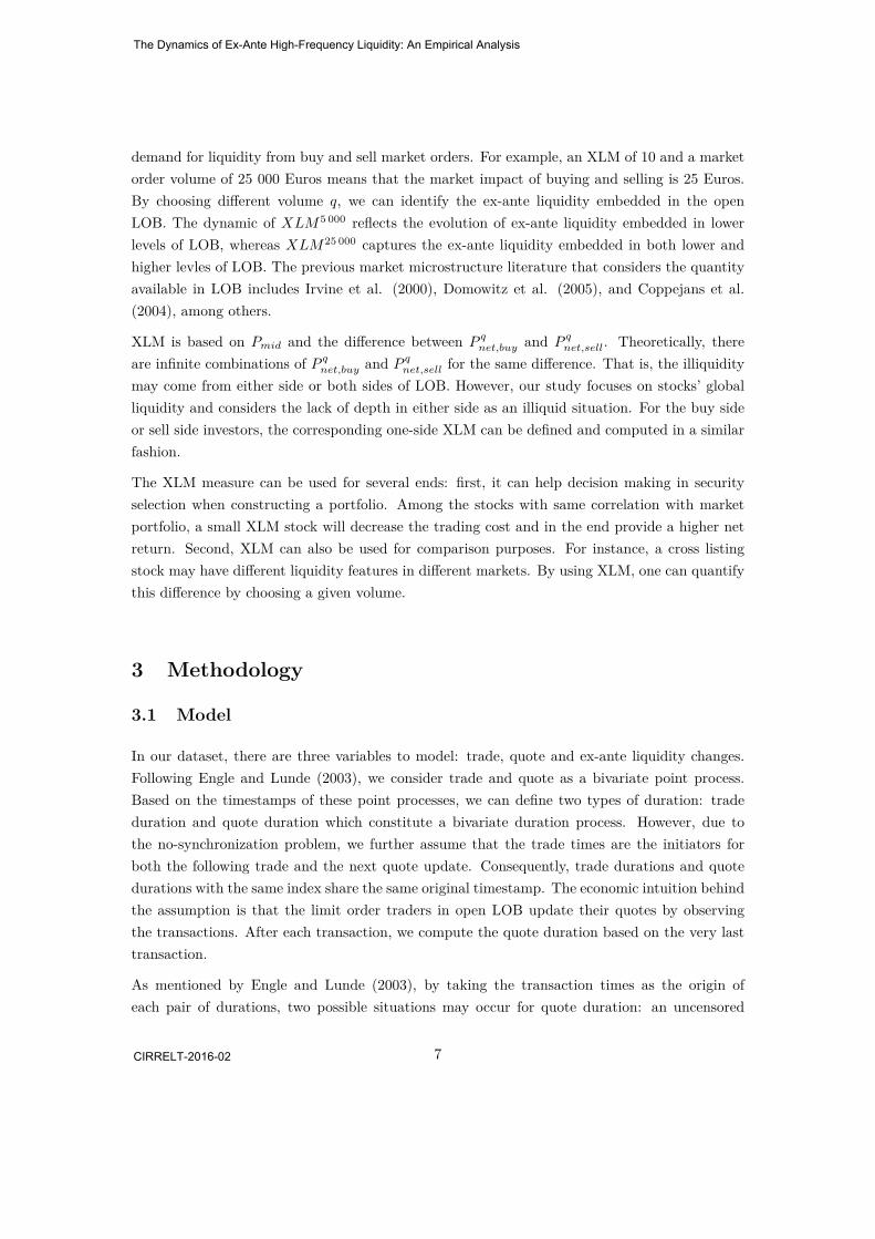
3 Methodology

3.1 Model

In our dataset, there are three variables to model: trade, quote and ex-ante liquidity changes.Following Engle and Lunde (2003), we consider trade and quote as a bivariate point process.Based on the timestamps of these point processes, we can define two types of duration: tradeduration and quote duration which constitute a bivariate duration process. However, due tothe no-synchronization problem, we further assume that the trade times are the initiators forboth the following trade and the next quote update. Consequently, trade durations and quotedurations with the same index share the same original timestamp. The economic intuition behindthe assumption is that the limit order traders in open LOB update their quotes by observingthe transactions. After each transaction, we compute the quote duration based on the very lasttransaction.

As mentioned by Engle and Lunde (2003), by taking the transaction times as the origin ofeach pair of durations, two possible situations may occur for quote duration: an uncensored

7


CIRRELT-2016-02

observation or a censored observation. The uncensored duration occurs when the quote updateis before the next trade arrival and the censored duration happens when the following tradearrives before the quote update. We denote xi and yi as the trade duration and quote duration,respectively, and further define the observed quote duration yi = (1 − di) · yi + dixi, wheredi = I{yi>xi}.

Apart from the time dimension, for our purposes, we have to model the liquidity dimension.We use the above mentioned XLM as the liquidity measure. In the uncensored situation, wetake the average of the measure within the first quote update timestamp and the following tradetimestamp. We propose that its evolution could be written as:

XLMqi = XLMq

0 +i∑

k=1Zk (2)

where Zk is defined as the kth rounded signed change for XLMq.

We define p as the joint density for trade duration, quote duration and XLMq changes. Wepropose the following decomposition for this joint density of kth mark:

p(xk, yk, zqk | Fk−1;ω)

= g(xk | Fk−1;ω1) · fDur(yk | xk, Fk−1;ω2) · fA(Ak | xk, yk, Fk−1;ω3)·

fD(Dk | xk, yk, Ak, Fk−1;ω4) · fS(Sk | xk, yk, Ak, Dk, Fk−1;ω5)

We define xk and yk as exogenous factors, which relate to the trade duration and observed quoteduration, for XLMq changes. Conditional on information set Fk−1 and two durations, Ak takeson value 0 or 1 indicating if there is a change on kth XLMq. Conditional on Ak = 1, Dk relatesto the direction of the XLMq change by taking on the value −1 and +1. Finally, given theinformation set (Fk−1, Ak = 1, Dirk), Sk takes on positive integers and indicates the size of thechange. ω relates to the parameter set including ω1, ω2, ω3, ω4 and ω5 which are the parametersfor factors of trade duration, observed quote duration, activity, direction and size.

We adopt the Log-ACD model originally introduced by Bauwens and Giot (2000) in modelingthe irregularly spaced trade durations which represents a main characteristic of high frequencydata:

xk

ψk= εk, ψk = exp

ω +p∑

j=1αjεk−j +

l∑j=1

βj lnψk−j + Ψ′Wk−1

(3)

where ψk = E(xk |Fk−1 ) and εk is a i.i.d random variable following the generalized gammadistribution with unit expectation. The process of duration is composed of a sequence of desea-sonalized durations. Wk−1 is a vector of exogenous variables available at k − 1 which includes

8


CIRRELT-2016-02

trade-related variables, quote-related variables and dummy variables to capture the intraday sea-sonality (hereafter, all exogenous vectors will include dummy variables to capture the intradayseasonality). We use the Log-ACD as it is more flexible in modeling and the positivity constrainton durations is always respected8 .

We adopt a similar structure for observed quote duration, that is

yk

φk= εk, φk = exp

µ+p∑

j=1ρjεk−j + ρj+1εk−1dk−1 +

l∑j=1

δj lnφk−j + Φ′Vk−1

(4)

where φk = E(yk |Fk−1 ) and εk is supposed to be i.i.d exponential distributed and the errordistribution is supported by the estimation convergence. In the equation, we add a term witha censored dummy variable to capture the impact of censored observation and the vector ofexogenous variables Vk−1 which may have some common variables with Wk−1. We show in thefollowing section that as quote durations are conditional on transactions, one possible exogenousvariable could be the expected trade duration available at tick k.

Regarding the liquidity dimension, we decompose the XLMq change into three factors: Activity,Direction and Size. The advantage of the decomposition approach is that we can use simpleand interpretable factors to model the different facets of liquidity. To this end, the first factor,Activity, is a bivariate variable that takes values of 0 or 1 to indicate whether there is a changein the XLMq measure. To model the activity factor, we use the auto-logistic model (Cox et al.,(1981)). As the log-likelihood function of the auto-logistic is concave, the numerical optimizationcan be easily and reliably realized. However, the high-frequency data often performs a slow decayfor longer lags in an autoregressive structure. Thus there is a trade-off between bias and variance,i.e., inference with too few parameters may be biased, while that with too many parametersmay cause precision and identification problems. To solve this, we adopt another structurecalled the GLARMA (Generalized Linear Autoregressive Moving Average) binary model whichis a generalized structure of auto-logistic structure allowing for moving average-type behavior(Shephard (1995)). The auto-logistic model for activity is defined as:

f (Ak = 1 |Fk−1, xk, yk ) = p(θAk ),where p(θA

k ) = exp(θAk )

1 + exp(θAk )

(5)

and θAk = Π′

AMAk−1 + gA

k , gAk =

p∑j=1

γAj g

Ak−j +

l∑j=1

λAj Ak−j

8 The ACD (Autoregression Conditional Duration ) model is initialized by Engle and Russell (1998) and widelyused for duration modeling.

9


CIRRELT-2016-02

Consequently, f(Ak = 0 |Fk−1, xk, yk ) = 11 + exp(θA

k )

where MAk−1 is the vector of exogenous variables for the activity factor known at k − 1. In this

logistic modeling, the parameter θAk is time-varying and depends on both its own lag variables,

such as lags of gk and Ak, and some exogenous variables. The model will be validated by applyingthe Ljung-Box test on the standardized errors defined by :

uAk = Ak − p(θA

k )√p(θA

k )(1− p(θAk ))

(6)

which should be uncorrelated with zero mean and unit variance.

In a similar way, the Direction of change of the liquidity measure conditional on the activityfactor is specified by another binary process on 1 or −1 (positive indicates that more liquiditycost should be paid when trading volume q and negative is related to less liquidity cost situation)and is estimated by another auto-logistic model:

f (Dk = 1 |Fk−1, xk, yk, Ak = 1) = p(θDk ),where p(θD

k ) = exp(θDk )

1 + exp(θDk )

(7)

and θDk = Π′

DMDk−1 + gD

k , gDk =

p∑j=1

γDj g

Dk−j +

l∑j=1

λDj Dk−j .

Consequently, f(Dk = −1 |Fk−1, xk, yk, Ak = 1) = 11 + exp(θD

k ).

MDk is a vector including exogenous variables of subset Fk−1and ΠD is a parameter vector. It

should be noted that the vectors MD and MA might have some identical exogenous variables.

Once the model is estimated, we use the Ljung-Box test to validate its ability to capture themain features of data. The test will be applied to standardized residuals:

uDk = Dk − (2p(θD

k )− 1)

2√p(θD

k )(1− p(θDk ))

(8)

Finally, the last factor is Size which captures the magnitude of the change of XLM. Less thanhalf of observations in the sample have no size change, that is, they stay at their previous level.Thus we will adopt a geometric process for size changes. The choice of geometric distribution ismotivated by its simplicity and generality:

Sk |Fk−1, xk, yk, Ak = 1) ∼ 1 + g(λk) (9)

10


CIRRELT-2016-02

λk = exp(θSizk )

1 + exp(θSizk )

,

θSizk = Π′

SizMSizk−1 + gSiz

k and gSizk =

p∑j=1

γSizj gSiz

k−j +l∑

j=1λSiz

j Sk−j

where MSizk−1 is a vector of exogenous variables and ΠSiz is the corresponding parameter vector.

g(λk) indicates the geometric distribution with parameter λk9. In order to capture the asymmetry

between up-move size and down-move size, we add a direction variable in the vector of exogenousvariables. In Equation (9), we add one to the geometric distribution since the minimum changeis one. We also apply the Ljung-Box statistics to standardized residuals to evaluate the model.Given the conditional distribution of Size, we have

E(Sk − 1 |Fk−1, xk, yk, Ak = 1)) = 1− λk

λk(10)

V ar(Sk − 1 |Fk−1, xk, yk, Ak = 1)) = 1− λk

(λk)2 . (11)

Standardized residuals are computed as

uSizk = Sk − 1− E(Sk − 1 |Fk−1, xk, yk, Ak = 1)√

V ar(Sk − 1 |Fk−1, xk, yk, Ak = 1)(12)

and an adequate modeling requires uSizk being uncorrelated with zero mean and unit variance.

In summary, for the estimation process, we can separately estimate each factor by using theMaximum Likelihood approach. The BIC criteria will be applied for the model selection, espe-cially for the choice of number of lags. Moreover, in order to test if the model captures the mainfeatures of time series data, we perform a portmanteau test in which residuals will be used tocalculate the Ljung-Box statistics as a measure of residual dependence.

Then, with the previous specifications, all the observations can be classified into one of the threefollowing categories:

1) There is no change in XLM, that is, activity factor Ak = 0 and no direction and size factors.

2) Liquidity decreases and the size change is at least one unit. The corresponding factors are :Ak = 1, Dk = 1, and Sk = sk;

3) Liquidity increases and size change is at least one unit. The corresponding factors are :Ak = 1, Dk = −1, and Sk = sk;

9The general probability distribution function is f(x = m) = λ(1− λ)m, 0 < λ < 1,m = 0, 1, 2, ...

11


CIRRELT-2016-02

The maximum likelihood estimation function is equal to :

L(ω1, ω2, ω3, ω4, ω5;xk, yk, zqk) =

=n∑

k=1

log[g(xk | Fk−1;ω1)] + log[fDur(yk | xk, Fk−1;ω2)]+Ik(1) · [log(fA(Ak | Fk−1;ω3))]+Ik(2) · [log(1− fA(Ak | Fk−1;ω3)) + log(fD(Dk | Fk−1;ω4)) + log(fS(Sk | Fk−1;ω5))]+Ik(3) · [log(1− fA(Ak | Fk−1;ω3)) + log(1− fD(Dk | Fk−1;ω4)) + log(fS(Sk | Fk−1;ω5))

(13)

where Ik(1), Ik(2), Ik(3) correspond to the indicator function relating to the three categoriesmentioned above.

To conclude, the advantage of this modeling is that the partition enables us to simplify themodeling and computation task by specifying the suitable econometric models for the marginaldensities of trade duration and conditional densities for quote duration and factors such asActivity, Direction and Size. In addition, for different purposes, the model could also be extendedto a more or less complicated context by including other factors. In these decomposition models,one of the crucial tasks is to identify the exogenous variables. Apart from the irregularly spacedduration, it is reasonable to test whether the rest of the factors also contain seasonality effects.

3.2 Exogenous Variables Set

Given the model defined above, we need to identify the possible exogenous variables, apart fromown lags, for each component. In this study, we attempt to find some variables that have economicinterpretation. In previous literature, the most widely used variables have been spread, tradingvolume and price (Hasbrouck (1996), Goodhart and O’Hara (1997), Coughenour and Shastri(1999) and Madhavan (2000)). The intuition is that trading activities and LOB trader behaviorare related. For instance, in a volatile trading period, trading volume will increase and tradeduration and quote duration will decrease. Consequently, these variations will generate a volatileopen LOB.

The first exogenous variable is relative spread change which is computed by the following formula:

RelativeSpreadk = 100 · (ln(askk)− ln(bidk))

Its variation is measured by:

DeltaSpreadk = RelativeSpreadk −RelativeSpreadk−1

where ask and bid are the best sell price and buy price available in open LOB. The advantage ofrelative spread is that it is dimensionless and can be used to directly compare different stocks.

As the relative spread captures quasi-instantaneous information and might be noisy, anotherspread-related variable is the average relative spread over the ten most recent observations:

12


CIRRELT-2016-02

AveSpreadk = 110

10∑i=1

RelativeSpreadk−i

Regarding the volume dimension, the first exogenous variable is the square root of the volume(number of shares), SquareRoot (vol), that initiates the current trade. There are two reasonsfor the use of square root, one is to weigh down the large trade volume, and the second isthat the price impact proves to be a concave function of market order size (Hasbrouck (1991)).If the volume that initiates the current trade is large, we expect a volatile situation and, byconsequence, the trade duration and quote duration are likely to be short.

The second volume-related variable should capture the imbalance of the signed trade. To thisend, we adopt the depth measure proposed by Engle and Lange (2001) which is defined as follows:

Abs(sign.vol)k =|10∑

i=1signk−ivolumek−i |

where the signk−i and volumek−i are the trade sign and trade volume for the (k − i)th trade.The trades are classified into buy-initiated and sell-initiated according to the rule of Lee andReady (1991). Intuitively, when the depth measure increases, it indicates that the trades areimbalanced and the market is dominated by one-sided pressure.

The third dimension is duration. We define two sorts of duration, back-quote duration andquote-quote duration, that are different from trade duration and quote duration. The formeris used to consider the duration between the first update of LOB after the previous trade andthe following trade which contains quote information. It should be noted that the back-quoteduration could be zero due to the fact that the quote duration might be censored when the tradeoccurs before the update of open LOB. The way by which the data is sampled ignores somequotes when there is more than one update between two trades. It might not be a concern when75% of the quotes are preserved as in Engle and Lunde (2003). However, in a market where theopen LOB is more active as in the Xetra trading system, ignoring the quote activity may be aconcern. In fact, only around 20% of the quotes are preserved in our dataset.

The quote-quote duration variable considers the duration for which there is no change of XLM.As a result, it will be used only in explaining the components such as direction and size whenthe liquidity measure changes.

The above variables will be all (or partially) included in the exogenous variable vectors fordifferent components. In addition, we also put time-of-day dummy variables in the vectors toremove the seasonality, a stylized fact in high-frequency data. There exist several techniquesto this end. In our study, we use eight time-of-day dummy variables to capture the intradayseasonality for each component for which we desire modeling: one for the first half hour afterthe market opens and then one for each hour of the trading day until the market closes.

Table 1 presents the summary statistics of durations and exogenous variables for the first week ofJuly 2010. The number of trades for all stocks ranges from 8 256 to 19 488. The trade frequency isalso confirmed by the corresponding average trade durations. That is, stocks with larger number

13


CIRRELT-2016-02

of trades correspond to shorter trade durations. Regarding the average trade volumes, there is abig difference: it varies from 5,180 to 15,472 Euros, meaning that the selected stocks have differentlevels of liquidity. The average quote durations are relatively small and there is evidence thatthe dynamics in the open LOB are more active than that of trades. Considering other exogenousvariables, it is natural to see that the averages of DeltaSpread and ∆XLM are close to zero. AsAveSpread is dimensionless, we can consider this variable as an indicator of transaction costs.All stocks have an average of AveSpread around 0.05%, meaning that the average spread remainsstable across the stocks. The average trade imbalance variable Abs(sign.vol) varies from 944 to3 616 shares, indicating the existence of different trading patterns across the stocks.

[Insert Table 1 here]

4 Estimation and results on liquidity

The data covers the first week of July 2010 and the last week of June 2011 for stocks RWE, MEO,MRK and TKA. We present and compare the estimation results for XLMq with potential sizeq of 5 000 and 25 000 Euros during the first week of July 201010. XLM5 000 and XLM25 000

represent ex-ante liquidities embedded in lower and higher levels of LOB, respectively. By takingdifferent potential sizes, we can examine the dynamics of lower- and higher- levels of LOB withvarious exogenous variables. The log-likelihood is maximized by the quadratic hill climbingmethod and the maximization program is run with Matlab v7.6.0 with Optimization Toolbox.

4.1 Temporal Factors

The estimation results of trade durations and quote durations are presented in Table 2 andTable 4. Panel A presents the estimation results for lagged dependent variables, and Panel B forexogenous variables. A more detailed analysis can be found in the Appendix. Table 3 and Table5 show the statistics related to estimations.

4.1.1 Trade Duration Factor

In the modeling, we decompose the explanatory variables of trade durations into two groups:lagged dependent variables and exogenous variables. More specifically, the lagged dependentvariables are used to capture the degree of persistence in the trade durations. One part of theexogenous variables will test the effect of different variables on trade durations, and the otherpart, with dummy variables, helps to remove seasonality.

10Results for potential size of 5 000 Euros for the same week are presented in the appendix. More results onother potential sizes and the other week are available upon request.

14


CIRRELT-2016-02

The overall results on trade durations, presented in Panel B of Table 2, are stable across stocksover the two sample periods and provide some new empirical evidence about trade durationdynamics. First, the sums of the coefficients for the first two lagged dependent variables arearound 0.9, suggesting that trade durations are highly persistent. Second, the coefficients forDeltaSpread and AveSpread are all positive and significant for the 4 stocks, showing thatwhen the liquidity decreases, traders will slow down their trading intensities. Moreover, thecoefficient for the short-term variable SquareRoot (vol) is negative and significant for the 4stocks, indicating that large trades will increase trading intensity. However, the coefficient forthe long-term variable Abs(sign.vol) is positive and significant only for RWE and TKA. Thismeans that, for these two stocks, when trade imbalance increases, the trading activity will slowdown. Third, trading durations do perform an intraday pattern.


The model is validated by the Ljung-Box statistics. Table 3 presents the results at different lagsfor trade durations and the standardized residuals of trade durations. The left side of the tableshows that there is a high persistence in autocorrelation of the trade duration dynamics. Theright side of the table presents evidence that the Log-ACD model is capable of removing thisautocorrelation feature in the trade durations since the Ljung-Box statistics have been reduceddramatically and, in most of cases, the hypothesis of no autocorrelation cannot be rejected.


4.1.2 Quote Duration Factor

Similar to the trade duration equation, we also decompose explanatory variables of the quoteduration equation into two parts: lagged dependent variables and exogenous variables. Weinclude more exogenous variables in the quote duration equation than in the trade durationequation since we assume that the trade durations are exogenous and can explain the quoteduration dynamics. More specifically, the exogenous variables we use in explaining the dynamicsof quote durations are: trade-duration-related variables, censored effect variable, DeltaSpread,AveSpread, SquareRoot (vol), Abs(sign.vol), BackQuote duration and 4XLM . Panel B ofTable 4 presents the corresponding estimate results.

The effect of exogenous variables on the quote duration can be briefly summarized as follows: first,spread-related variables, such as DeltaSpread and AveSpread, and the volume-related variableSquareRoot (vol) have negative impact on the quote durations. This suggests that when thespread is large and the trading volume is high, LOB traders speed up their revisions. Second,the coefficient for the trade imbalance variable Abs(sign.vol) is positive for MEO, RWE andTKA, and is negative for MRK. The positive coefficient of Abs(sign.vol) is not very intuitive if

15


CIRRELT-2016-02

we consider trade imbalance as a result of information asymmetry. One explanation might be thatthe positive effect is evidence of high-frequency algorithmic trading. The algorithmic (probablynot human) traders may benefit from providing liquidity by creating this trade imbalance. Forexample, if an algorithmic trader wants to buy a given quantity of stocks, on the ask side he canplace limit orders in different price levels with different quantities. As a result, the pressure onthe sell side increases and then more trades occur on the bid side. In this case, there is no fearrelated to informed traders, and so quote revision can be postponed.


In Table 5, we find that the Ljung-Box statistics have been largely reduced and, in most of cases,the hypothesis of no autocorrelation cannot be rejected. It should be noted that, despite the largenumber of lagged variables, TKA still has a relatively high autocorrelation in the standardizedresiduals.


4.2 Liquidity Activity Factor

Up to now, we have analyzed the dynamics of trade durations and quote durations. Condi-tional on the these temporal variables, we can make further analysis on other dimensions ofliquidity. As we mentioned above, we decompose the change of the liquidity measure XLM intothree components: Activity, Direction and Size. Similar to the time dimension, we also puttwo groups of explanatory variables into the activity equation: lagged dependent variables andexogenous variables. TheMA vector includes expected trade duration, expected quote duration,DeltaSpread, AveSpread, SquareRoot (vol), Abs(sign.vol), BackQuote duration, 4XLM anddummy variables.

Table 6 and Table A.5 report the estimated results of the liquidity activity equation forXLM25 000

and XLM5 000. The activity process is a binary process in which the value 1 means a changein the liquidity measure XLM. To model the activity factor, we adopt the GLARMA structureintroduced by Rydberg and Shephard (2003). In addition to the GLARMA structure, we alsoinclude exogenous variables. Panel A of Table 6 presents the estimated results of the GLARMApart. For all stocks, we use a lag set of (1,2) to capture the autocorrelation of the activityfactor. Consistent with previous literature, the coefficients of the “GLAR” part are positive andsignificant, ranging from 0.66 to 0.95. The result suggests a high persistence in autocorrelationfor the activity factor. More specifically, there is a cluster effect in activity, namely, the changeof liquidity is more likely to be followed by another change.


16


CIRRELT-2016-02

In this study, we are also interested in the effect of exogenous variables on the dynamics ofliquidity. Panel B of Table 6 shows the estimated results for these exogenous variables. Forthe time dimension variables, expected trade duration and expected quote duration do not havethe same effect on the probability of liquidity change. In particular, a longer expected tradeduration increases the probability of liquidity change, whereas a longer quote duration decreasesthis probability. The same effects are also found for the activity factor of XLM5 000. In thetick-by-tick trading framework, as found by Dionne et al. (2009) and Dionne et al. (2015), alonger trade duration will have a positive impact on price volatility. As a result, a longer tradeduration will increase the probability of liquidity change. On the other hand, quote durationmeasures the quote intensity. A longer quote duration means a less active open LOB. Becauseof this, the quote is likely to be unchanged.

Regarding spread-related variables, both DeltaSpread and AveSpread have a positive effect onthe probability of liquidity change. These two measures are related to liquidity itself. Whenliquidity decreases, LOB traders are more prudential in their quotes, and are more likely toupdate their quotes. Therefore, the probability of liquidity change increases. Recall that, inthe trade duration equation, DeltaSpread and AveSpread also have a positive effect on tradeduration. We find that different types of traders have different ways to protect themselves. Moreconcretely, when the market is less liquid, market order traders become less active and LOBtraders become more active and careful. It should be noted that the activity factor only tells uswhether the liquidity changes or not; there is no information on the direction and magnitude ofchange.

Regarding volume-related variables, SquareRoot (vol) and Abs(sign.vol) affect the probabilityof liquidity change in different ways. The coefficients of SquareRoot (vol) are both significantat a 5% level for XLM5 000 and XLM25 000 changes. However, the signs of the coefficients areopposite (positive for XLM25 000 changes and negative for XLM5 000 changes). The resultssuggest that the large trades are likely to increase the probability of high level liquidity changes.As mentioned before, large trades are likely to be informative. Under this circumstance, the LOBtraders are more likely to review their high-level quotes and then the resulted high-level liquiditychanges. On the other side, low-level liquidity is likely to be insensitive to high trade volumes.One possible explanation is that low-level LOB is competitive and features a quick resilience. Asin the trade duration equation and quote duration equation, the effect of Abs(sign.vol) is againnot clear. Only one stock has a significant coefficient. The results suggest that the probability ofliquidity change hardly depends on the long-run trade imbalance. Possible explanations are that:First, Abs(sign.vol) captures information on the last ten trades and the activity component hasa very short memory. Second, algorithm traders might provide liquidity by “creating” this tradeimbalance.

Another time dimension variable, BackQuote duration, also has a positive impact on the prob-ability of liquidity change. This is in line with the estimate results for trade duration. As we can

17


CIRRELT-2016-02

see from Panel B of Table 6, the effect of expected trade duration is higher than that of expectedquote duration. Therefore, the longer BackQuote duration implies a more volatile market andliquidity is likely to be updated. For the liquidity measures XLM5 000 and XLM25 000, as ex-pected, the coefficient is positive and significant at a 5% level. This means that when a stock isless liquid, there is more chance that LOB traders review their quote and then the liquidity ofthis stock changes. Concerning the dummy variables, we find that there is a seasonality patternonly for some stocks in certain time periods; most of the periods do not exhibit a seasonalitypattern. The results are shown in Panel C of Table 6.

Similar to trade durations and quote durations, we use the Ljung-Box statistics to validate themodel. The statistics for the activity factor and the corresponding standardized residuals arereported in the left side and right side of Table 7, respectively. On the one hand, the activityfactor is highly autocorrelated. At five-lag level, the Ljung-Box statistics range from 358 to 1127for all stocks and the hypothesis of no autocorrelation is rejected at any confidence level. On theother hand, we find that the model which includes the GLARMA part and exogenous variablescan capture this autocorrelation feature very well. On the right side of the table, all statisticshave been reduced to less than the critical values except one for MRK.


4.3 Liquidity Direction Factor

Another component of liquidity measure is direction which is also a binary process: the value 1means a decrease of liquidity and -1 means an increase of liquidity. Conditional on the activityfactor, the direction factor gives more information about the change of XLM. To capture thedynamics of direction, we use a similar variables set as for the other equations. Three stocks takethe GLARMA(2,1) structure and one stock takes the GLARMA(3,1). Panel A of Table 8 andTable A.5 illustrate the estimation results for the GLARMA structure. Interestingly, the sums ofthe “MA” part are all negative and smaller than -0.5, indicating a mean-reverting feature. Thatis, the increase of liquidity is likely to be followed by a decrease of liquidity, and vice versa.


The exogenous variables we include in the direction equation are: QuoteQuote duration,DeltaSpread, AveSpread, SquareRoot (vol), Abs(sign.vol), BackQuote duration and 4XLM .Panel B of Table 8 and Table A.5 present the estimated results of these exogenous variables. Inthe direction equation, the new variable QuoteQuote duration is defined as the duration betweentwo liquidity measure changes. As the direction component is observed only when the activityfactor is equal to one, it is more reasonable to use a temporal variable to capture this time interval.Based on Panel B of Table 8 for XLM25 000, we find that three stocks have a positive coefficientfor QuoteQuote duration and only one is significant. It appears that QuoteQuote duration is

18


CIRRELT-2016-02

not a relevant variable in predicting the direction factor. The same results are also found forXLM5 000.

Considering the spread related variables, a highDeltaSpread increases the probability of liquiditydecrease when there is a liquidity change. Intuitively, when the spread increases, this meansthe LOB traders keep away from mid-quotes, and so XLM is likely to increase. Compared toDeltaSpread, the AveSpread has the opposite effect on the direction factor. This suggests thatthe permanent increase of the spread will indeed increase the probability of liquidity increase. Itseems evident that when the traders have to pay a higher liquidity premium, the LOB traders(i.e, liquidity providers) are willing to provide liquidity.

Regarding the volume-related variables, the coefficient of SquareRoot (vol) is positive forXLM25 000

meaning that the current large trades predict a less liquid situation for a large trade, which isconsistent with previous literature. Intuitively, the large trade is likely to be informed tradewhich will create volatility in the market. Accordingly, when LOB traders are likely to keepaway from mid-quotes, and so the liquidity will decrease. However, as shown in Table A.7,SquareRoot (vol) has no effect on the low level liquidity direction factor, suggesting that lowlevel liquidity is less sensitive to trade volumes. The trade imbalance variable Abs(sign.vol) hasno significant effect on the direction factor for both XLM5 000 and XLM25 000 changes. Thisconfirms the results for the activity component. There is no clear impact of Abs(sign.vol) onliquidity change, therefore the effect of Abs(sign.vol) on direction is not clear. As we focus onthe dynamics of liquidity measure XLM, the reason to the lack of information content of tradeimbalance is out of our scope. However, it might be interesting for trading strategy analysis oralgorithm trading analysis to continue exploring this aspect.

Another temporal variable, BackQuote duration, has a positive impact on the probability ofliquidity increase. This suggests that when trades become less active, the LOB traders are likelyto review their quotes and incite trades by providing more liquidity. Regarding liquidity measureXLM5 000 and XLM25 000, an increase of XLM will increase the probability of being liquid. Thisis the evidence of the mean-reverting in XLM dynamics. As for the other components, we alsouse dummy variables to capture seasonality in the direction factor. The estimated results showthat the coefficients are not significant, meaning that there is not a clear seasonality effect onthe direction factor. The results for coefficients of dummy variables are presented in Panel C ofTable 8.

The direction factor is observed when the liquidity measure XLM changes. The Ljung-Boxstatistics for the direction factor and corresponding standardized residuals are reported in Table9, respectively. Similar to the activity factor, the direction factor is highly autocorrelated. Thehypothesis of no autocorrelation is rejected at any confidence level for all stocks. That is, theLjung-Box statistics for standardized residuals from 5 to 200 lags are not significant at a 5%level.


19


CIRRELT-2016-02

4.4 Liquidity Size Factor

The last factor is the size of liquidity change. Table 10 and Table A.9 report the estimatedresults for both XLM25 000 and XLM5 000 changes. Panel A of Table 10 shows the results ofthe GLARMA part. We find that the number of lags of the GLARMA part ranges from (2,1) to(2,2). Depending on the stock, the effect of lagged value is either positive or negative. As shownin equation 10, a higher λk indicates a smaller expectation of size factor. Combined with theestimated results of the direction component, the implication is that XLM does have a mean-reverting feature, however, the magnitude of reverting varies from one stock to another. Similarresults are found in Table A.9 for size factor of XLM5 000 changes.


The exogenous variables are the same as in the equation for the liquidity direction factor. Inaddition, we include current direction and lagged direction in the size equation. In total, thereare nine exogenous variables in the size equation. Panel B of Table 10 and Table A.9 reportthe estimated results of exogenous variables for XLM25 000 and XLM5 000, respectively. Oncewe have all results for liquidity activity, direction and size factor, we can closely analyze theentire effect of exogenous variables on every dimension of liquidity changes. Table 12 presentsand compares the effects of key exogenous variables on XLM25 000 and XLM5 000 changes andliquidity measures.

In line with the estimated results for the direction factor, QuoteQuote duration does not havea significant effect on all stocks with respect to both XLM25 000 and XLM5 000 changes. Recallthat QuoteQuote duration is the duration between two XLM changes. Again, it indicates thatthe LOB structure has a short memory and does not have the power to predict dynamic of sizechange.

As shown in Panel B of Table 10, there exists a leverage effect. That is, the negative size factorchange (less liquid) is higher than that of positive change (more liquid). Consistent with Rydbergand Shephard (2003), the current direction variable has negative and significant impact on theλk, which implies a higher expected liquidity change when liquidity decreases, and confirms theleverage effect for both XLM25 000 and XLM5 000 changes. However, the lagged direction is lesssignificant than the current one.

The temporal variable BackQuote duration has positive and significant effect on λk for bothXLM25 000 and XLM5 000 changes, indicating that even though the liquidity provider tries toincite the traders to trade by increasing the liquidity provision (our conclusion from the resultsof the direction equation), the magnitude of liquidity increase is moderated. On the other side,if the trading intensity increases and then the BackQuote duration decreases, the liquidity islikely to decrease with a greater magnitude.

20


CIRRELT-2016-02

The last exogenous variable 4XLM itself has a negative and significant effect on λk for bothXLM25 000 and XLM5 000 changes. This suggests a quick resilience in liquidity. If the market isevaluated previously as less liquid based on XLM, the actual liquidity is prone to increase andthe size of this increase is likely to be large. On the other side, if the market is evaluated asliquid by the XLM, the actual liquidity is likely to decrease with a moderated size factor.

We also attempt to test if there is a seasonality in the size factor by using dummy variables. Asshown in Panel C of Table 10, similar to activity and direction factors, there is little seasonalityfeature in size component because most of the coefficients are not significant from zero at a 5%level.

As for the direction factor, the size factor is also observed when the liquidity measure XLMchanges. Table 11 reports the Ljung-Box statistics of the size factor and the correspondingstandardized residuals. Interestingly, the statistics for the size factor vary significantly acrossthe stocks. For instance, the size factors of RWE and TKA, with Ljung-Box statistics of 1406and 889 for 5 lags, are relatively high autocorrelated. Given the high Ljung-Box statistics ofstandardized residuals for stocks RWE and TKA at small lags (from 5 lags to 20), the modelmight have a misspecification problem on θSiz

k or a mild distributional failure. It should benoted that θSiz

k can be specified in many different ways and the distribution for size factor candiffer from geometric distribution. However, a parsimonious and interpretable model is alwayspreferred.


4.5 Summary of Estimation

Up to now, we can compare the total effect on liquidity from different exogenous variables. Table12 summarizes and compares the effect of key exogenous variables on XLM25 000 and XLM5 000.The spread-related variable, DeltaSpread, has positive impact on λk: three stocks are significantfor XLM5 000 and only one for XLM25 000. It suggests that the size factor of XLM5 000 is moresensitive to the changes in the spread than that of XLM25 000. Combined with the results ofthe direction factor, it shows that when previous spread increases, the actual liquidity is likelyto decrease. Furthermore, the size of this decrease in liquidity is expected to be small. However,if the previous DeltaSpread is small, the actual liquidity is likely to increase with a higher sizefactor. There exists an asymmetry in the effect on the size factor of the liquidity changes.


Panel B and C of Table 12 also compare the different effect of the same exogenous variables onXLM25 000 and XLM5 000 changes. AveSpread has a negative significant effect on λk for TKA

21


CIRRELT-2016-02

with respect to XLM25 000 changes and a positive effect for RWE and TKA with respect toXLM5 000 changes. The implication is that the dynamics of liquidity only has a short memory.Combined with the results of the direction equation, the negative effect of AveSpread on λk

suggests that high AveSpread will lead to a more liquid situation for both XLM25 000 andXLM5 000 changes. However, the magnitude of this increase in liquidity is larger for XLM25 000

changes than that ofXLM5 000 changes. On the other hand, if the AveSpread is small, the actualliquidity will decrease and the magnitude of this decrease in liquidity is smaller for XLM25 000

changes than that of XLM5 000 changes.

Relative to the size factor of XLM25 000 changes, SquareRoot (vol) is not significant for threestocks but significant for TKA11. However, SquareRoot (vol) has a significant positive effect onall the stocks with respect to the size factor of XLM5 000 changes, confirming high resiliency atlower levels of LOB. Our model also quantifies the effect of trade quantity on liquidity change.As for the effect of volume on XLM25 000, a high trading volume predicts a decrease of liquiditywith a high magnitude for TKA. For the other stocks, liquidity change seems limited to one unit,whereas a low trading volume will lead to an increase of liquidity with a smaller magnitude.Interestingly, XLM5 000 is less sensitive to high trading volume than XLM25 000. That is, ahigh trading volume does not increase the liquidity change probability and the magnitude ofthe liquidity change. However, a small trading volume is likely to increase the liquidity changeprobability and the magnitude of this change. This is evidence that liquidity providers at alow-level of LOB are more sensitive to the small trading volumes which are usually issued frompredetermined trading strategies.

As shown in Panel B and C of Table 12, the effect of the trade imbalance variable Abs(sign.vol)is not significant for size factors for both XLM5 000 and XLM25 000 changes. Moreover, forXLM5 000 changes, there is no effect of imbalance on each of the three factors, confirming the lackof informativeness of trade imbalance. Concerning the XLM25 000 changes, given the negativeeffect of Abs(sign.vol) on the direction factor, it suggests that if there is an imbalance in theprevious trades, liquidity is likely to increase in a moderated fashion.

5 Conclusion

After the introduction of the open LOB trading mechanism, trading frequency has become higherthan ever before. By consequence, liquidity has become an important issue for active traders,investors and financial institutions. This paper analyzes of the dynamics of ex-ante liquidity

11 Recall that the value of the size component is defined as the size change minus one. Therefore, the nonsignif-icance means that the size component changes less than one unit.

22


CIRRELT-2016-02

changes. The ex-ante liquidity measures used in this study are XLM25 000 and XLM5 000 pro-posed by the Xetra trading system. Different from an ex-post liquidity measure, the XLM is anex-ante volume dependent measure. The computation of the measure requires information suchas the prices and the corresponding quantity available in the open LOB.

To model the dynamics of the liquidity changes, we adopt the decomposition approach proposedby Rogers and Zane (1998). The liquidity changes have been decomposed into five factors: tradedurations, quote durations, activity, direction and size. Trade durations and quote durationsare temporal variables and are not synchronized. To manage this problem, we follow Engleand Lunde (2003) by defining the last trade time as the initial quote time in quote durationcomputation. The other three factors are directly related to the change of XLM itself. Boththe activity factor and the direction factor are binary processes taking the value 0 and 1, or -1and 1, respectively. The size factor captures the magnitude of XLM change. To investigate thedynamics of each component, we apply the relevant econometric models to each factor and puta wide range of trade-related exogenous variables into the models. These include volume-relatedvariables, trade-balance-related variables and temporal variables. The models are validated bythe t-test of the coefficients and the Ljung-Box test on the deduced standardized residuals.

By including different microstructure based variables, we first find that most trade-related vari-ables can influence the dynamic of both trade and quote durations. Moreover, the quote durationsare influenced by the dynamics of trade durations, trade-related variables and 4XLM . Second,expected trade durations and quote durations are likely to affect the probability of liquiditychange. Most the trade-related variables have an impact on the activity factor except the long-run trade imbalance variable, Abs(sign.vol). Third, the temporal variable QuoteQuote durationdoes not seem to have an impact on the direction factor. Fourth, there is a leverage effect in thesize factor, that is, the magnitude of liquidity decrease is higher than that of increase. Amongthe trade-related variables, only spread change has a significant effect on the size factor forXLM25 000 and XLM5 000 changes. SquareRoot (vol) has a very different effect on XLM25 000

and XLM5 000 changes, suggesting a high resilence at the lower levels of LOB. Fifth, the tradedurations and quote durations have an obvious seasonality pattern, whereas the seasonality pat-tern for other factors is not clear. Overall, we provide evidence that trade durations and quotedurations have an impact on ex-ante liquidity. Other exogenous variables that affect ex-ante liq-uidity include DeltaSpread, AveSpread, SquareRoot (vol), BackQuote duration and 4XLM .

Future research can continue in several directions. Our study focuses on the impact of trade-related variables on liquidity changes. A possible alternative is to investigate how liquidity changeco-moves with trades. Another direction is to decompose the liquidity changes in a different orderor into different factors to answer other microstructure questions. It could also be interesting togeneralize the model from one particular stock to a portfolio. Again, the unsynchronization ofthe trade durations and quote durations between different stocks is a challenge. It will require amore complicated econometric model and reasonable assumptions.

23


CIRRELT-2016-02

Figure 1: Timestamps for trades and quote update in open LOB

This figure presents the temporal relation between trades and quote updates. The trades and the quote updates arepresented by circles and squares, respectively.

Figure 2: Intraday Seasonality Pattern For Trade Durations

This figure presents the intraday patterns of seasonality variables for trade durations for different stocks.

24


CIRRELT-2016-02

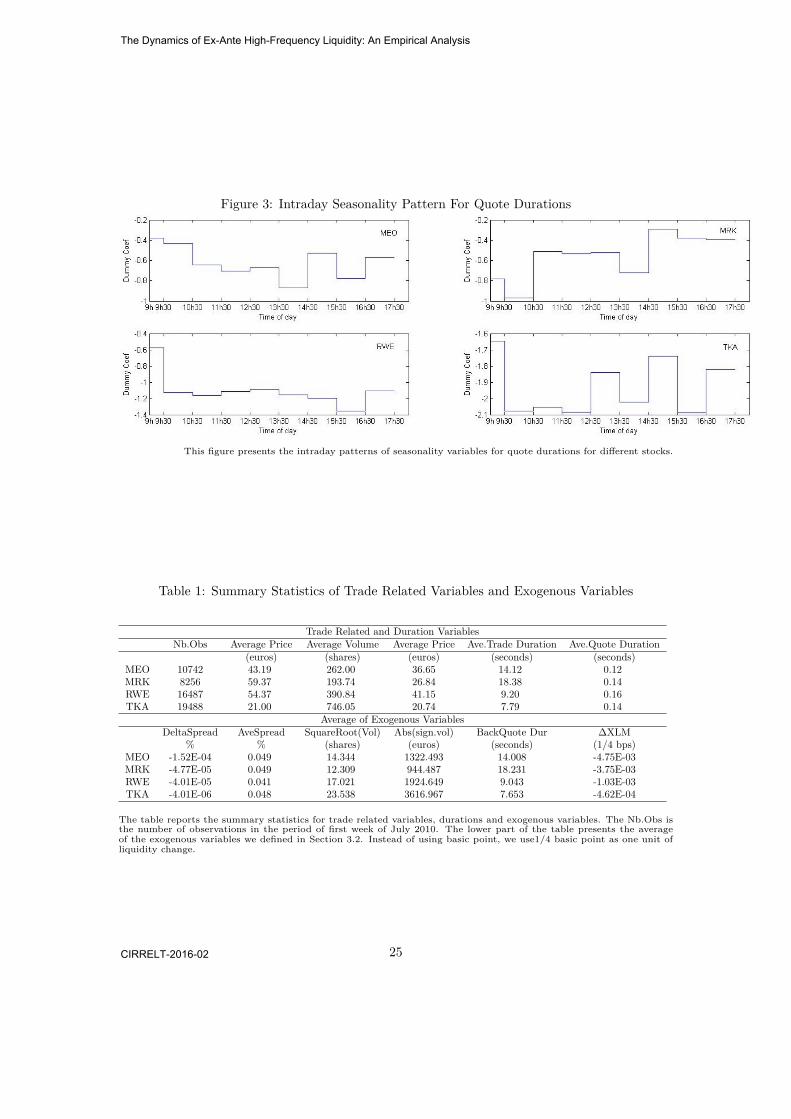
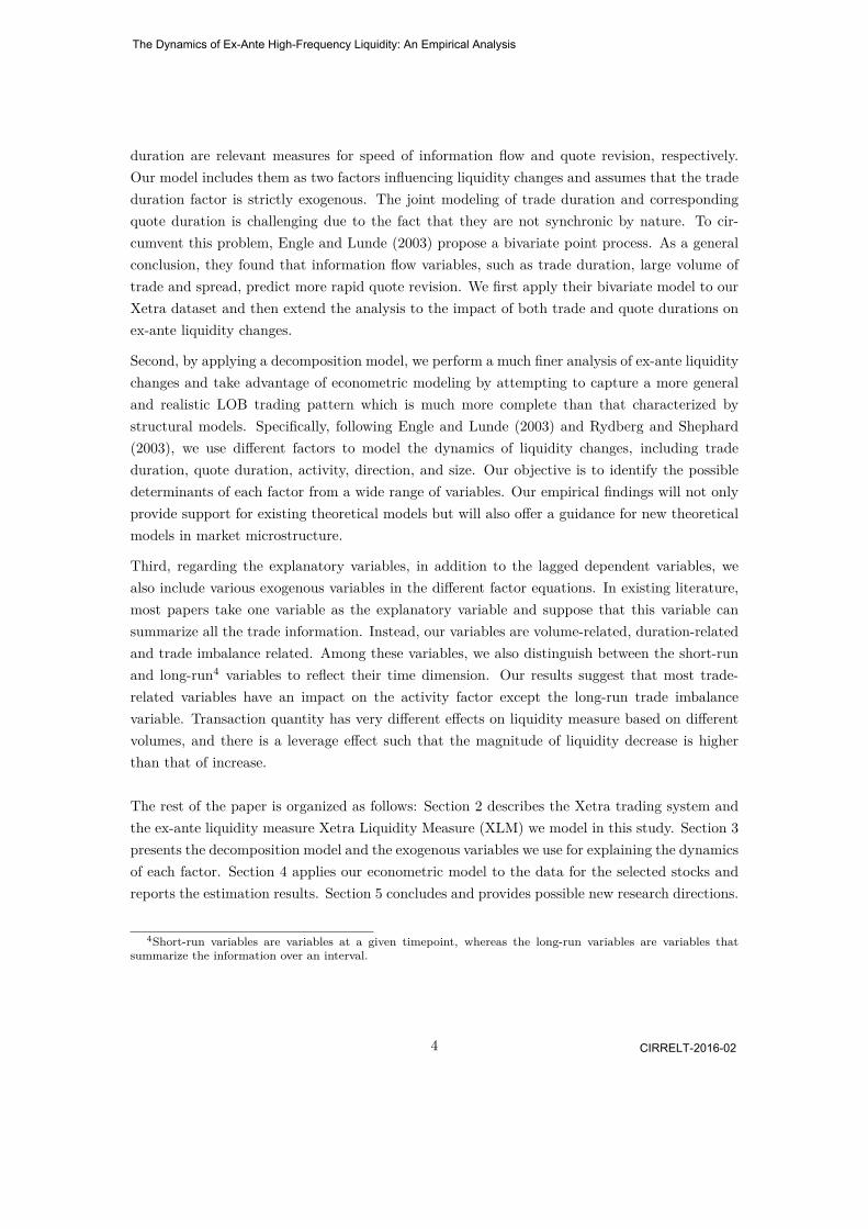
Figure 3: Intraday Seasonality Pattern For Quote Durations

This figure presents the intraday patterns of seasonality variables for quote durations for different stocks.

Table 1: Summary Statistics of Trade Related Variables and Exogenous Variables

Trade Related and Duration VariablesNb.Obs Average Price Average Volume Average Price Ave.Trade Duration Ave.Quote Duration

(euros) (shares) (euros) (seconds) (seconds)MEO 10742 43.19 262.00 36.65 14.12 0.12MRK 8256 59.37 193.74 26.84 18.38 0.14RWE 16487 54.37 390.84 41.15 9.20 0.16TKA 19488 21.00 746.05 20.74 7.79 0.14

Average of Exogenous VariablesDeltaSpread AveSpread SquareRoot(Vol) Abs(sign.vol) BackQuote Dur ΔXLM

% % (shares) (euros) (seconds) (1/4 bps)MEO -1.52E-04 0.049 14.344 1322.493 14.008 -4.75E-03MRK -4.77E-05 0.049 12.309 944.487 18.231 -3.75E-03RWE -4.01E-05 0.041 17.021 1924.649 9.043 -1.03E-03TKA -4.01E-06 0.048 23.538 3616.967 7.653 -4.62E-04

The table reports the summary statistics for trade related variables, durations and exogenous variables. The Nb.Obs isthe number of observations in the period of first week of July 2010. The lower part of the table presents the averageof the exogenous variables we defined in Section 3.2. Instead of using basic point, we use1/4 basic point as one unit ofliquidity change.

25


CIRRELT-2016-02

Table 2: Estimated Results For Trade Durations

MEO MRK RWE TKAEst STD T-Stat Est STD T-Stat Est STD T-Stat Est STD T-Stat

Panel A

ln(dur(lag1)) 0.875 0.04 21.904 0.804 0.04 19.958 0.975 0.026 37.655 1.194 0.037 32.168ln(dur(lag2)) -0.021 0.034 -0.627 0.126 0.056 2.239 -0.13 0.037 -3.481 -0.306 0.062 -4.969ln(dur(lag3)) 0.063 0.021 2.958 0.024 0.038 0.629 0.11 0.027 4.045 0.094 0.033 2.848x/phi (lag1) 0.081 0.008 10.057 0.06 0.006 9.96 0.119 0.007 17.467 0.13 0.009 14.863x/phi (lag2) -0.059 0.009 -6.81gamme1 0.512 0.021 24.364 0.515 0.024 21.552 0.974 0.026 36.793 0.798 0.019 42.379gamme2 0.78 0.052 15.077 0.711 0.054 13.17 0.35 0.014 25.582 0.449 0.016 27.562cons 0.239 0.033 7.147 0.111 0.027 4.128 0.052 0.016 3.282 0.008 0.007 1.087

Panel B

delta spread 14.848 0.276 53.892 26.521 0.937 28.303 18.192 0.6 30.336 14.341 0.556 25.782lev.spread 1.146 0.187 6.119 1.232 0.226 5.444 0.807 0.176 4.597 0.488 0.084 5.777

square root(vol) -0.013 0.001 -9.499 -0.008 0.002 -5.075 -0.008 0.001 -12.042 -0.003 0 -9.700abs(sign.vol) 4.51E-06 4.94E-06 0.913 3.45E-06 7.05E-06 0.489 4.54E-06 1.64E-06 2.768 1.24E-06 5.30E-07 2.340

Back_quote_dur 3.90E-04 5.53E-04 0.705 8.17E-04 3.25E-04 2.512 -0.002 0.001 -3.337 -0.002 3.92E-04 -3.9714XLM 0.019 0.014 1.404 -0.012 0.013 -0.902 0.019 0.007 2.488 0.001 0.013 0.109

Panel C

Dummy1 0.043 0.024 1.773 -0.112 0.02 -5.492 -0.002 0.011 -0.156 -0.021 0.006 -3.690Dummy2 -0.003 0.016 -0.174 -0.066 0.013 -5.191 0.049 0.008 5.925 -0.002 0.004 -0.574Dummy3 0.03 0.015 1.991 -0.015 0.012 -1.294 0.04 0.009 4.549 0.007 0.004 1.900Dummy4 0.063 0.018 3.542 -0.002 0.012 -0.144 0.041 0.009 4.513 0.023 0.005 4.757Dummy5 0.05 0.016 3.165 -0.008 0.014 -0.593 0.082 0.011 7.743 0.037 0.006 6.512Dummy6 0.051 0.017 2.939 -0.021 0.012 -1.713 0.069 0.01 7.228 0.03 0.006 4.683Dummy7 0.011 0.013 0.885 -0.002 0.012 -0.189 0.056 0.009 6.502 0.028 0.005 5.315Dummy8 -0.039 0.011 -3.404 -0.004 0.011 -0.365 -0.001 0.007 -0.088 0.005 0.004 1.202

The table reports the estimated results for trade durations. Panel A presents the results for Log-ACD part, Panel Bincludes the results for the exogenous variables and Panel C consists of the results for dummy variables. Bold entriesindicate the coefficients are significant at a 5% level.

Table 3: Ljung-Box Statistics For Trade Durations and Deduced Standardized Residuals

Ljung-Box Statistics on Trade Durations Ljung-Box Statistics on Corresponding Standardized ResidualsLags MEO MRK RWE TKA C_Value Lags MEO MRK RWE TKA C_Value5 557.17 412.26 1722.03 1721.64 11.07 5 3.55 4.29 3.80 1.35 11.0710 975.85 762.70 2671.13 2906.49 18.31 10 8.26 7.53 13.16 10.17 18.3115 1192.88 1087.96 3434.51 3849.18 25.00 15 9.97 9.12 17.60 19.12 25.0020 1430.56 1404.29 4117.37 4500.64 31.41 20 11.27 12.38 24.02 29.27 31.4150 3167.19 3137.33 7234.72 7743.76 67.50 50 45.86 44.97 90.65 51.34 67.50100 5164.17 5240.23 11234.36 13131.06 124.34 100 102.40 70.91 178.10 95.96 124.34150 6445.61 6632.65 13539.18 17527.54 179.58 150 168.24 106.01 246.26 162.45 179.58200 7350.44 7601.17 15641.54 21028.11 233.99 200 234.11 131.46 316.12. 228.84 233.99

The table reports the Ljung-Box statistic on trade durations (left side) and standardized residuals of trade duration(right side) for different stocks at different lags.The column of Lags is the number of lags we use to compute the statisticand the C_Value is the critical value for the corresponding lags.

26


CIRRELT-2016-02

Table 4: Estimated Results For Quote Durations


Panel A

ln(dur(lag1)) 0.299 0.004 70.792 0.309 0.006 52.986 0.301 0.004 75.553 0.199 0.005 39.587ln(dur(lag2)) 0.041 0.004 9.511 0.131 0.004 29.611 0.127 0.004 35.714 0.023 0.004 5.949ln(dur(lag3)) 0.165 0.003 48.008 0.017 0.004 4.831x/phi (lag1) 0.072 0.001 57.179 0.042 0.001 31.149 0.063 0.001 51.643 0.047 0.001 42.350x/phi (lag2) 0.021 0.001 22.672x/phi (lag3) 0.017 0.001 17.146x/phi (lag4) 0.016 0.001 23.487

cons -0.575 0.016 -36.725 -0.394 0.012 -31.852 -1.110 0.013 -83.628 -1.821 0.017 -106.145

Panel B

x/phi (lag1)*dummy 0.070 0.004 19.370 0.069 0.005 13.471 0.075 0.004 18.651 0.071 0.003 25.239trade_dur/expected_trade_dur 0.154 0.002 70.405 0.269 0.003 107.065 0.267 0.002 108.278 0.254 0.002 105.179

lag_trade_dur/expected_trade_dur 0.037 0.003 12.023 -0.001 0.002 -0.584 0.026 0.003 8.439 0.091 0.003 34.055lag_expected_trade_dur 0.108 0.005 23.294 -0.064 0.003 -18.381 0.202 0.004 46.566 0.226 0.004 51.182

delta spread -10.671 0.176 -60.510 -12.345 0.187 -66.007 -13.301 0.116 -114.931 -8.662 0.090 -95.923lev.spread -4.573 0.098 -46.586 -1.560 0.109 -14.254 -9.825 0.116 -84.423 -5.026 0.106 -47.236

square root(vol) -0.072 3.72E-04 -193.950 -0.065 0.001 -125.819 -0.040 1.82E-04 -219.646 -0.029 1.69E-04 -170.569abs(sign.vol) 9.73E-05 1.69E-06 57.550 -3.51E-05 2.80E-06 -12.525 2.82E-05 1.10E-06 25.673 2.96E-05 7.10E-07 41.690

Back_quote_dur 6.68E-04 1.94E-04 3.444 0.004 1.14E-04 35.804 0.010 2.83E-04 35.118 0.001 3.08E-04 2.637ΔXLM -0.074 0.002 -36.090 -0.033 0.002 -17.847 -0.023 0.002 -14.136 0.012 0.003 4.697

Panel C

Dummy1 0.193 0.011 17.960 -0.390 0.012 -33.898 0.531 0.010 55.626 0.173 0.010 17.074Dummy2 0.139 0.007 19.935 -0.577 0.009 -65.518 -0.018 0.006 -3.088 -0.258 0.007 -36.187Dummy3 -0.067 0.006 -11.290 -0.115 0.008 -15.127 -0.055 0.006 -8.858 -0.231 0.007 -31.943Dummy4 -0.128 0.006 -20.111 -0.141 0.009 -15.891 -0.003 0.007 -0.506 -0.266 0.010 -27.010Dummy5 -0.097 0.006 -15.359 -0.131 0.009 -15.115 0.021 0.007 2.790 -0.020 0.009 -2.186Dummy6 -0.298 0.007 -43.491 -0.329 0.007 -45.212 -0.047 0.008 -6.227 -0.201 0.011 -17.957Dummy7 0.049 0.005 9.788 0.101 0.008 12.343 -0.089 0.006 -13.938 0.081 0.008 9.593Dummy8 -0.203 0.005 -41.558 0.015 0.008 1.795 -0.245 0.006 -44.364 -0.268 0.007 -36.236

The table reports the estimated results for quote durations. Panel A presents the results for Log-ACD part, Panel Bincludes the results for the exogenous variables and Panel C consists of the results for dummy variables. Bold entriesindicate the coefficients are significant at a 5% level.

Table 5: Ljung-Box Statistics For Quote Durations and Deduced Standardized Residuals

Ljung-Box Statistics on Trade Durations Ljung-Box Statistics on Corresponding Standardized ResidualsLags MEO MRK RWE TKA C_Value Lags MEO MRK RWE TKA C_Value5 120.09 34.11 297.78 492.92 11.07 5 10.43 5.92 8.1 8.12 11.07010 134.80 42.80 369.75 611.70 18.31 10 15.54 15.96 9.87 49.33 18.30715 164.76 52.64 392.25 687.89 25.00 15 24.77 23.1 11.25 72.68 24.99620 181.16 63.90 424.92 727.08 31.41 20 45.75 32.93 12.38 116.32 31.41050 278.87 117.19 650.20 952.42 67.50 50 74.21 47.55 53.54 251.1 67.505100 408.87 169.94 1019.39 1373.74 124.34 100 151.98 91.85 131.14 345.85 124.342150 559.91 212.97 1200.21 1623.94 179.58 150 220.29 128.82 178.94 441.45 179.581200 664.12 257.83 1373.35 2121.54 233.99 200 278.68 172.9 217.33 518.5 233.994

The table reports the Ljung-Box statistic on quote durations (left side) and standardized residuals of quote duration(right side) for different stocks at different lags.The column of Lags is the number of lags we use to compute the statisticand the C_Value is the critical value for the corresponding lags.

27


CIRRELT-2016-02

Table 6: Estimated Results For Liquidity Activity Factor of XLM25 000


Panel A

g(t− 1) 0.661 0.084 7.837 0.848 0.053 15.933 0.762 0.041 18.459 0.954 0.016 59.194activity(t− 1) 0.807 0.042 19.351 0.892 0.049 18.153 0.776 0.034 22.695 0.399 0.029 13.564activity(t− 2) -0.359 0.102 -3.534 -0.657 0.087 -7.514 -0.410 0.062 -6.651 -0.345 0.033 -10.517

cons -2.023 0.107 -18.962 -2.031 0.143 -14.196 -1.479 0.102 -14.492 -1.384 0.101 -13.745

Panel B

Expect Trade Dur 0.269 0.035 7.735 0.278 0.033 8.529 0.220 0.029 7.471 0.143 0.025 5.852Expect Quote Dur -0.097 0.020 -4.934 -0.086 0.021 -4.117 -0.124 0.022 -5.611 -0.016 0.013 -1.245


square root(vol) 0.026 0.003 9.192 0.035 0.004 8.876 0.004 0.002 2.132 0.008 0.001 7.517abs(sign.vol) 1.52E-05 1.82E-05 0.834 4.05E-05 3.13E-05 1.293 -7.21E-06 0.000 -0.755 -1.54E-05 4.34E-06 -3.541

Back_quote_dur 0.006 7.36E-04 8.027 0.004 6.40E-04 7.010 0.006 1.19E-03 4.959 0.005 9.99E-04 4.526ΔXLM 0.037 0.013 2.945 0.062 0.012 5.162 0.071 0.009 7.852 0.076 0.015 5.129

Panel C

Dummy1 0.190 0.134 1.418 0.028 0.134 0.211 -0.051 0.089 -0.574 0.174 0.071 2.464Dummy2 -0.084 0.087 -0.966 -0.205 0.090 -2.272 -0.097 0.065 -1.500 0.038 0.052 0.729Dummy3 -0.096 0.084 -1.152 -0.042 0.093 -0.452 -0.075 0.066 -1.141 0.104 0.056 1.862Dummy4 -0.193 0.093 -2.067 -0.224 0.097 -2.310 -0.140 0.066 -2.132 -0.065 0.064 -1.013Dummy5 -0.133 0.089 -1.503 -0.192 0.107 -1.799 -0.243 0.082 -2.981 -0.020 0.073 -0.273Dummy6 -0.096 0.093 -1.036 -0.103 0.098 -1.053 -0.219 0.077 -2.844 0.011 0.074 0.153Dummy7 -0.122 0.074 -1.659 -0.315 0.095 -3.322 -0.136 0.067 -2.026 -0.083 0.064 -1.298Dummy8 -0.034 0.064 -0.534 -0.112 0.088 -1.270 -0.033 0.055 -0.605 0.084 0.051 1.650

The table reports the estimated results for Activity factor. Panel A presents the results for GLARMA part, Panel Bincludes the results for the exogenous variables and Panel C consists of the results for dummy variables.Bold entriesindicate the coefficients are significant at a 5% level.

Table 7: Ljung-Box Statistics For Activity Factor of XLM25 000 and Deduced Standardized Residuals


The table reports the Ljung-Box statistic on activity factor (left side) and standardized residuals of activity factor (rightside) for different stocks at different lags.The column of Lags is the number of lags we use to compute the statistic andthe C_Value is the critical value for the corresponding lags.

28


CIRRELT-2016-02

Table 8: Estimated Results For Direction Factor of XLM25 000


Panel A

g(t− 1) 1.06 0.07 14.77 0.90 0.10 9.28 0.94 0.07 13.97 0.50 0.02 26.64g(t− 2) -0.30 0.06 -4.72 -0.14 0.08 -1.65 -0.30 0.09 -3.45 0.03 0.02 1.61g(t− 3) 0.08 0.04 1.73

direction(t− 1) -0.57 0.05 -10.77 -0.55 0.06 -9.11 -0.67 0.04 -14.95 -1.70 0.04 -42.55cons 0.04 0.11 0.38 -0.13 0.13 -0.98 -0.06 0.09 -0.71 0.18 0.09 2.09

Panel B

Expect QuoteQuote Dur -0.01 0.01 -1.25 0.02 0.01 1.51 0.01 0.01 1.32 0.02 0.01 2.52delta spread 4.84 1.03 4.70 3.05 1.12 2.73 2.40 0.95 2.54 2.75 0.73 3.79lev.spread -5.37 1.37 -3.91 -1.14 1.91 -0.60 -3.00 1.64 -1.83 -7.11 0.98 -7.24

square root(vol) 1.15E-02 4.07E-03 2.82 7.88E-04 0.01 0.15 4.18E-03 2.41E-03 1.73 7.14E-03 1.82E-03 3.92abs(sign.vol) -3.51E-05 2.52E-05 -1.39 6.55E-05 4.01E-05 1.64 -4.53E-06 1.34E-05 -0.34 -1.63E-05 7.23E-06 -2.25

Back_quote_dur -2.97E-03 8.40E-04 -3.54 -1.15E-03 6.75E-04 -1.70 -0.01 1.25E-03 -4.61 -3.49E-03 1.62E-03 -2.15ΔXLM -0.33 0.02 -14.10 -0.22 0.02 -9.52 -0.29 0.02 -14.65 -0.13 0.02 -6.82

Panel C

Dummy1 0.11 0.17 0.62 -0.12 0.17 -0.71 0.23 0.12 1.88 0.06 0.11 0.61Dummy2 0.01 0.13 0.05 0.20 0.12 1.64 0.12 0.09 1.33 -0.10 0.09 -1.10Dummy3 0.07 0.12 0.60 0.07 0.12 0.56 0.22 0.09 2.47 0.06 0.09 0.61Dummy4 0.16 0.13 1.18 0.03 0.13 0.20 0.14 0.09 1.54 -0.13 0.11 -1.18Dummy5 0.05 0.13 0.36 0.10 0.15 0.69 0.10 0.11 0.94 0.00 0.12 0.02Dummy6 0.02 0.13 0.17 -0.08 0.13 -0.63 0.20 0.10 1.91 -0.16 0.12 -1.32Dummy7 0.10 0.11 0.92 0.09 0.13 0.71 0.15 0.09 1.65 -0.22 0.11 -1.93Dummy8 0.09 0.10 0.90 -0.04 0.12 -0.34 0.09 0.08 1.17 -0.08 0.09 -0.83

The table reports the estimated results for Direction factor. Panel A presents the results for GLARMA part, Panel Bincludes the results for the exogenous variables and Panel C consists of the results for dummy variables. Bold entriesindicate the coefficients are significant at a 5% level.

Table 9: Ljung-Box Statistics For Direction Factor of XLM25 000 and Deduced Standardized Residuals


The table reports the Ljung-Box statistic on direction factor (left side) and standardized residuals of direction factor(right side) for different stocks at different lags.The column of Lags is the number of lags we use to compute the statisticand the C_Value is the critical value for the corresponding lags.

29


CIRRELT-2016-02

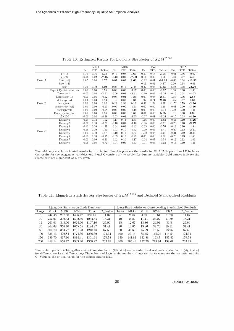
Table 10: Estimated Results For Liquidity Size Factor of XLM25 000


Panel A

g(t-1) 0.70 0.16 4.36 0.79 0.08 9.60 0.59 0.15 3.95 -0.01 0.36 -0.02g(t-2) -0.16 0.02 -7.45 -0.13 0.02 -7.90 0.14 0.09 1.61 0.18 0.07 2.48

Size (t-1) 0.07 0.04 1.77 0.07 0.03 2.66 -0.22 0.01 -16.83 -0.49 0.04 -13.92Size (t-2) 0.11 0.03 3.37 0.00 0.18 -0.01

cons 0.39 0.10 4.04 0.28 0.11 2.44 0.42 0.08 5.43 1.90 0.08 23.29

Panel B

Expect QuoteQuote Dur 0.00 0.00 0.56 0.00 0.00 -1.87 0.00 0.00 -0.97 0.00 0.00 -1.50Direction(t) -0.07 0.03 -2.51 -0.06 0.03 -2.31 -0.10 0.02 -5.27 -0.15 0.04 -4.02Direction(t-1) -0.01 0.05 -0.12 0.06 0.04 1.26 0.09 0.03 2.71 0.15 0.06 2.58delta spread 1.03 0.53 1.93 1.16 0.87 1.33 1.97 0.71 2.76 0.25 0.37 0.68lev.spread 0.96 1.05 0.92 0.22 1.36 0.16 0.39 1.24 0.31 -1.76 0.75 -2.36

square root(vol) 0.00 0.00 -0.67 0.00 0.00 -0.71 0.00 0.00 1.31 -0.01 0.00 -3.16abs(sign.vol) 0.00 0.00 -0.08 0.00 0.00 -0.19 0.00 0.00 -0.74 0.00 0.00 -1.41

Back_quote_dur 0.00 0.00 1.58 0.00 0.00 1.60 0.01 0.00 5.35 0.01 0.00 4.38ΔXLM -0.01 0.02 -0.28 -0.03 0.02 -1.95 -0.07 0.01 -5.28 -0.15 0.03 -4.30

Panel C

Dummy1 -0.13 0.13 -1.02 -0.17 0.13 -1.33 -0.16 0.09 -1.83 -0.54 0.10 -5.26Dummy2 -0.07 0.10 -0.72 -0.10 0.09 -1.10 -0.05 0.06 -0.71 -0.26 0.10 -2.72Dummy3 -0.12 0.10 -1.21 -0.04 0.09 -0.43 -0.05 0.06 -0.76 -0.19 0.10 -1.94Dummy4 -0.16 0.10 -1.59 -0.03 0.10 -0.32 -0.09 0.06 -1.41 -0.29 0.12 -2.51Dummy5 0.06 0.10 0.57 -0.10 0.11 -0.87 -0.02 0.08 -0.21 -0.31 0.12 -2.51Dummy6 -0.10 0.10 -0.95 -0.09 0.10 -0.99 0.03 0.08 0.36 -0.20 0.13 -1.50Dummy7 -0.03 0.09 -0.33 -0.02 0.10 -0.17 -0.04 0.07 -0.58 -0.12 0.12 -1.03Dummy8 -0.06 0.08 -0.72 -0.04 0.09 -0.43 -0.01 0.06 -0.23 -0.14 0.10 -1.41

The table reports the estimated results for Size factor. Panel A presents the results for GLARMA part, Panel B includesthe results for the exogenous variables and Panel C consists of the results for dummy variables.Bold entries indicate thecoefficients are significant at a 5% level.

Table 11: Ljung-Box Statistics For Size Factor of XLM25 000 and Deduced Standardized Residuals


The table reports the Ljung-Box statistic on size factor (left side) and standardized residuals of size factor (right side)for different stocks at different lags.The column of Lags is the number of lags we use to compute the statistic and theC_Value is the critical value for the corresponding lags.

30


CIRRELT-2016-02

Table 12: Effect of Key Exogenous Variables on XLM

Panel A: Effects on XLM5000 and XLM25000 changes

Activity Direction Size (magnitude) Total Effect on Ex-ante Liquidity

Delta spread + (4,4) + (4,4) + (4,1) If the previous spread increases (less liquid), the liquidity is likely to decrease,the size of this decrease in liquidity is likely to be small.

Lag XLM + (4,4) - (3,4) - (2,2) If the market is less liquid, the following liquidity is likely to increase and thesize of this increase will be large.

Direction(t) - (3,4) Leverage effect: the size of liquidity decrease is larger than liquidity increase.Panel B: Effect on XLM25000 changes

Activity Direction Size Total Effect on Ex-ante Liquidity

Ave_spread + (3) - (2) - (1) If Ave_Spread increases, the liquidity is likely to increase, the size of thisincrease is likely to be large.

Square root(vol) + (4) + (2) - (1) If the trade volume increases, the liquidity is likely to decrease, the size ofthis decrease is likely to be large.

Abs(sign.vol) - (1) - (1) #If imbalance of trade increases, the liquidity is likely to remain the same, ifthe liquidity changes, it will increase and imbalance does not affect the size ofthe change.

Panel C: Effect on XLM5000 changes

Activity Direction Size Total Effect on Ex-ante Liquidity

Ave_spread + (3) - (2) + (2) If Ave_Spread increases, the liquidity is likely to increase, the size of thisincrease is likely to be moderate.

Square root(vol) - (3) # + (4) If the trade volume increases, the liquidity is likely to remain the same, if theliquidity changes, the size of this change is likely to be small.

Abs(sign.vol) - (1) # # If imbalance of trade increases, the liquidity is likely to remain the same, theimbalance of trades does not affect the size of the change.

The table summarizes the effect of various exogenous variables on the XLM5 000and XLM25 000 changes, # relates to anon-significant estimated coefficient at a 5% level. In panel A, + (4,4) means that four stocks have significantly positivecoefficients for XLM5000 changes and four for XLM25000 changes.

31


CIRRELT-2016-02

ReferencesAitken, M., Comerton-Forde, C., 2003. How should liquidity be measured? Pacific-Basin FinanceJournal 11 (1), 45–59.

Bauwens, L., Giot, P., 2000. The Logarithmic ACD Model: An Application to the Bid-Ask QuoteProcess of Three NYSE Stocks. Annals of Economics and Statistics / Annales d’Économie etde Statistique (60), 117–149.

Beltran-Lopez, H., Giot, P., Grammig, J., 2009. Commonalities in the order book. FinancialMarkets and Portfolio Management 23 (3), 209–242.

Beltran-Lopez, H., Grammig, J., Menkveld, A. J., 2011. Limit order books and trade informa-tiveness. The European Journal of Finance, 1–23.

Biais, B., Wooley, P., 2011. High frequency trading. Unpublished working paper. University ofToulouse, Industrial Economics Institute, Toulouse, France.

Bilodeau, Y., 2013. Xetraparser [computer software]. HEC Montréal.

Black, F., 1971. Toward a fully automated stock exchange. Financial Analysts Journal 27 (4),28–44.

Bloomfield, R., O’hara, M., Saar, G., 2015. Hidden liquidity: Some new light on dark trading.The Journal of Finance 70 (5), 2227–2274.

Boehmer, E., Saar, G., Yu, L., 2005. Lifting the veil: An analysis of pre-trade transparency atthe nyse. The Journal of Finance 60 (2), 783–815.

Brogaard, J., Hendershott, T., Riordan, R., 2014. High-frequency trading and price discovery.Review of Financial Studies.

Coppejans, M., Domowitz, I., Madhavan, A., 2004. Resiliency in an automated auction. Workingpaper, ITG Group.

Coughenour, J., Shastri, K., 1999. Symposium on market microstructure: A review of empiricalresearch. Financial Review 34 (4), 1–27.

Cox, D. R., Gudmundsson, G., Lindgren, G., Bondesson, L., Harsaae, E., Laake, P., Juselius, K.,Lauritzen, S. L., Jan. 1981. Statistical Analysis of Time Series: Some Recent Developments[with Discussion and Reply]. Scandinavian Journal of Statistics 8 (2), 93–115.

Demsetz, H., 1968. The Cost of Transacting. Quarterly Journal of Economics 82 (1), 33–53.

Dionne, G., Duchesne, P., Pacurar, M., 2009. Intraday value at risk (ivar) using tick-by-tick datawith application to the toronto stock exchange. Journal of Empirical Finance 16 (5), 777–792.

Dionne, G., Pacurar, M., Zhou, X., 2015. Liquidity-adjusted intraday value at risk modelingand risk management: An application to data from deutsche borse. Journal of Banking andFinance 59, 202 – 219.

Domowitz, I., Hansch, O., Wang, X., 2005. Liquidity commonality and return co-movement.Journal of Financial Markets 8 (4), 351–376.

Easley, D., O’Hara, M., 1987. Price, trade size, and information in securities markets. Journal ofFinancial Economics 19 (1), 69–90.

32


CIRRELT-2016-02

Engle, R. F., Lange, J., 2001. Predicting VNET: A model of the dynamics of market depth.Journal of Financial Markets 4 (2), 113–142.

Engle, R. F., Lunde, A., 2003. Trades and Quotes: A Bivariate Point Process. Journal of FinancialEconometrics 1 (2), 159–188.

Engle, R. F., Russell, J. R., 1998. Autoregressive Conditional Duration: A New Model forIrregularly Spaced Transaction Data. Econometrica 66 (5), 1127–1162.

Foucault, T., 1999. Order flow composition and trading costs in a dynamic limit order market.Journal of Financial Markets 2 (2), 99–134.

Foucault, T., Kadan, O., Kandel, E., 2005. Limit Order Book as a Market for Liquidity. Reviewof Financial Studies 18 (4), 1171–1217.

Giot, P., Grammig, J., 2006. How large is liquidity risk in an automated auction market? Em-pirical Economics 30 (4), 867–887.

Glosten, L. R., Harris, L. E., 1988. Estimating the Components of the Bid Ask Spread. Journalof Financial Economics 21 (1), 123.

Goodhart, C. A. E., O’Hara, M., 1997. High frequency data in financial markets: Issues andapplications. Journal of Empirical Finance 4 (2-3), 73–114.

Hasbrouck, J., 1991. Measuring the Information Content of Stock Trades. The Journal of Finance46 (1), 179–207.

Hasbrouck, J., 1996. Order characteristics and stock price evolution An application to programtrading. Journal of Financial Economics 41 (1), 129–149.

Hasbrouck, J., Saar, G., 2013. Low-latency trading. Journal of Financial Markets 16 (4), 646 –679, high-Frequency Trading.

Hausman, J. A., Lo, A. W., MacKinlay, A. C., 1992. An ordered probit analysis of transactionstock prices. Journal of Financial Economics 31 (3), 319–379.

Hendershott, T., Jones, C., Menkveld, A., 2011. Does algorithmic trading improve liquidity?The Journal of Finance 66 (1), 1–33.

Hendershott, T., Riordan, R., 2013. Algorithmic trading and the market for liquidity. Journal ofFinancial and Quantitative Analysis 48, 1001–1024.

Irvine, P. J., Benston, G. J., Kandel, E., 2000. Liquidity Beyond the Inside Spread: Measuringand Using Information in the Limit Order Book. SSRN eLibrary.

Jones, C., 2012. What do we know about high frequency trading? Unpublished working paper.Columbia University.

Lee, C. M. C., Ready, M. J., Jun. 1991. Inferring Trade Direction from Intraday Data. TheJournal of Finance 46 (2), 733–746.

Madhavan, A., 2000. Market microstructure: A survey. Journal of Financial Markets 3 (3),205–258.

Manganelli, S., 2005. Duration, volume and volatility impact of trades. Journal of FinancialMarkets 8 (4), 377–399.

33


CIRRELT-2016-02

McCulloch, R. E., Tsay, R. S., 2001. Nonlinearity in High-Frequency Financial Data and Hier-archical Models. Studies in Nonlinear Dynamics & Econometrics 5 (1), 1–17.

Menkveld, A. J., 2013. High frequency trading and the new market makers. Journal of FinancialMarkets 16 (4), 712 – 740, high-Frequency Trading.

O’Hara, M., 2015. High frequency market microstructure. Journal of Financial Economics 116 (2),257 – 270.

Parlour A., C., 1998. Price Dynamics in Limit Order Markets. The Review of Financial Studies11 (4), 789.

Riordan, R., Storkenmaier, A., 2012. Latency, liquidity and price discovery. Journal of FinancialMarkets 15 (4), 416 – 437.

Rogers, L. C. G., Zane, O., 1998. Designing and estimating models of high-frequency data.Unpublished paper.

Russell, J., Engle, R., 2005. A Discrete-State Continuous-Time Model of Financial TransactionsPrices and Times: The Autoregressive Conditional Multinomial-Autoregressive ConditionalDuration Model. Journal of Business & Economic Statistics 23 (2), 166.

Rydberg, T. H., Shephard, N., Mar. 2003. Dynamics of Trade-by-Trade Price Movements: De-composition and Models . Journal of Financial Econometrics 1 (1), 2–25.

Shephard, N., 1995. Generalized linear autoregressions. Working paper, Nuffield College, Uni-versity of Oxford.

Viswanathan, S., Wang, J. J. D., 2002. Market architecture: limit-order books versus dealershipmarkets. Journal of Financial Markets 5 (2), 127–167.

34


CIRRELT-2016-02

Appendix

1. Trade Duration Factor

Panel A of Table 2 presents the estimated results of the lagged dependent variables for all thestocks in the sample. The ACD-related models are based on the ARMA structure, meaning thatthe determinant parts of the dynamics of durations are specified by the lagged duration andlagged error term 1. As we expected, the trade durations of all stocks are highly autocorrelated.Taking the models’ efficiency and parsimony into consideration, the number of lagged tradedurations varies from one to three. The sum of the coefficients of lagged trade durations for allstocks is around 0.9, which confirms a very high degree of persistence in autocorrelation. TKAhas the most persistent trade durations among all stocks and has been specified by Log-ACD(3,2)dynamics. Regarding the error terms for all stocks, the parameters Gamma1 (ranges from 0.512to 0.974) and Gamma2 (ranges from 0.350 to 0.780) are small, indicating that the distributionof the random part is abrupt and near to zero; that is, expected trade duration shocks are verysmall.

Considering the exogenous variables mentioned above, we put six such variables in the trade dura-tion equations: DeltaSpread, AveSpread, SquareRoot (vol), Abs(sign.vol), BackQuote duration,and4XLM . Panel B of Table 2 reports the estimation results. Consistent with Engle and Lunde(2003), for all the stocks, a positive DeltaSpread, increases the trade duration. The parametersare all positive and significant at a 5% level. Intuitively, when the stocks become less liquid,traders will slow their trading intensities, and trading durations will become longer. Contrary toEngle and Lunde (2003), we find a positive sign for AveSpread coefficient. That is, the higherthe AveSpread is, the longer the trade durations are. The difference between DeltaSpread andAveSpread is that the former captures the short-run spread change and the latter relates tothe long-term spread change. It reveals that trade intensity is sensitive for both short-run andlong-run spread change. When the stocks become less liquid, traders slow down their activitiesand then wait for the moment when liquidity increases.

Another important exogenous variable is volume-related. For all stocks, the coefficients ofSquareRoot (vol) are all negative and significant at a 5% level. This means that large tradeswill generate higher trading intensity and shorter trade durations. According to Easley andO’Hara (1987), large trades are likely to be related to information trade because the informedtraders try to exploit their information advantage by increasing both the trading intensity andtrading quantity. Another volume-related variable is Abs(sign.vol) which measures the volumeimbalance (in shares) of the last ten trades (a higher value means a higher level of imbalanceand a zero value means a completely balanced trading activity). All stocks have small positive

1 Regarding the model selection, the first criteria is the Ljung-Box statistics, and the second one is the BICcriteria for the selection of number of lags.

35


CIRRELT-2016-02

coefficients, and only two of them are significant at a 5% level. The measure of imbalance alsorelates to information trading. Our results suggest that when the trades become imbalanced, thetrade intensity will decrease. Presumably, when the non-informed traders observe an imbalancedtrading history, they will then slow down their trading activity to protect themselves.

Regarding the BackQuote duration, we find that the effect of duration between the first quoteand the following trade on the trade duration is not clear. Two stocks have a positive signand two others have a negative sign. Moreover, three of them are significant at a 5% level.Intuitively, the trade activity should be positively correlated with quote activity. As a result,the coefficient should have a positive sign. Our results do not seem to be completely consistentwith this intuition. One explanation might be that trade duration consists of quote durationwhile BackQuote duration depends on both trade duration and quote duration. Therefore,the explanatory power of BackQuote duration is also influenced by quote duration, which iscensored. For instance, a longer BackQuote duration could be either a long trade duration ora shorter quote duration. The longer trade duration has a positive impact on trade duration,whereas a shorter quote duration has a negative one. Therefore, the sign of BackQuote durationon trade duration could be positive or negative.

The last exogenous variable is the change of liquidity measure XLM. Like DeltaSpread, a highXLM means a less liquid situation. If we follow the same argument as DeltaSpread, higher XLMwill decrease the trade intensity and then generate a longer trade duration. Our estimated resultsshow that 4XLM25 000 of RWE and 4XLM5 000 of MEO and TKA have positive estimatedcoefficients which are significant at a 5% level. This suggests that the 4XLM is likely to havea moderated effect on trade duration. However, if we combine the 4XLM result with that ofDeltaSpread, it suggests that the trade activity is more sensitive to the first level of LOB andthe quote activities beyond the first level are not likely to explain the trade duration dynamics.

The last part consists of dummy variables. Panel C of Table 2 reports the estimated results forthese dummy variables. To make the results more visible, we piecewisely plot the coefficient ofdummy variables in Figure 2. In line with previous literature, the trade durations do have adiurnal pattern. For all stocks, there is an inverse U-shaped pattern for trade durations.

2 Quote Duration Factor

Panel A of Table 4 reports the estimated results of lagged dependent variables for all stocks.Similar to trade durations, quote durations are also highly persistent. The number of laggedvalues varies from two to three and the number of lagged error terms varies from one to four.TKA features the most persistent dynamics and takes a Log-ACD(3,4) model to fit its dynamics.Comparing the Log-ACD model to the traditional ARMA structure, the sum of the coefficientof the “AR” part in the quote duration equation varies from 0.239 to 0.505. The relatively smallcoefficients can be explained by the fact that the start point of our quote duration is the tradetimestamp. When there is more than one update between two trades, only the first one is usedto calculate the quote duration. To some extent, this sampling “deletes” some autocorrelation

36


CIRRELT-2016-02

in quote durations. Regarding the coefficients of the error term, the estimated coefficients varyfrom 0.042 to 0.072, confirming the sampling effect in autocorrelation.

The censored effect is captured by the product of the censored dummy variable and the laggederror term. The censored effect is positive and significant at a 5% level for all stocks. Theimplication is that if the last quote duration is censored, the next quote duration is likely to belonger and censored again. Trade duration related variables consist of current error term, laggederror term and lagged expected trade duration. The estimated results show that the current errorterm and expected trade duration have a positive and significant effect on the quote durations.It suggests that when the (current and lagged) trade duration innovations and expected tradedurations are high, the quote duration will become longer. Intuitively, as quote activity adjuststo trade activity, trade duration and quote duration are correlated positively.

The spread-related variables, DeltaSpread and AveSpread, have a negative impact on the quotedurations, which is opposite to the trade duration. The coefficients are negative and significantat 5% level for all stocks. Spread variables are very important in explaining the trade activityand quote activity. It suggests that when the spread is large, the market order traders and LOBtraders react differently. Market order traders slow down their trading speed when observing anincreasing spread, whereas LOB traders speed up to update their price or quantity of limit orders.For an intraday LOB trader, a major concern is adverse selection. By attentively monitoring thechange of spread, LOB traders attempt to avoid this risk by updating their quote rapidly.

The effect of volume-related variables, SquareRoot (vol) and Abs(sign.vol), on quote duration issimilar to that of trade duration. More specifically, large trades predict shorter quote durations.As mentioned above, large trades relate to informed trades. Informed traders exploit short-lived information by increasing trade intensity and trade quantity. When trades become moreintensive, so do quote revisions. As a result, the quote durations become shorter. Regardingimbalanced measures Abs(sign.vol), their coefficients are all positive but only two of them aresignificant. Compared to SquareRoot (vol), Abs(sign.vol) is a long-run variable, as it consistsof information over the last ten trades. In a high-frequency trading framework, trades andinformation are short-lived. The estimated results suggest that the short-run measure is morepredictive than the long-run measure.

The BackQuote duration has a positive and significant impact on the following quote duration.A longer BackQuote duration can be either a low trade intensity or a high quote intensity. Thatis, a long trade duration or a short quote duration. Moreover, a long trade duration implies a longquote duration. The estimated results suggest that the long trade duration effect dominates theshort quote duration effect. Concerning the effect of liquidity measure XLM25 000, empirically,the effect is negative and significant at a 5% level for three stocks. One stock has a positivesignificant sign. We obtain similar results for XLM5 000. Theoretically, there are argumentsto support either sign. A high XLM reveals a more risky situation, especially a high adverseselection risk. LOB traders speed up their quote revisions to reduce this kind of risk. This

37


CIRRELT-2016-02

is more pronounced for less liquid stocks. On the other side, the increase of XLM will slowdown the trade activity and then the quote activity. Panel C of Table 4 reports the results ofestimation for dummy variables. We also find a seasonality effect for quote durations. However,because the quote durations are censored and the trade durations enter into the model of quotedurations, the seasonality pattern for quote durations is not like that of trade durations. Figure3 illustrates the intraday seasonality pattern for different stocks.

Table A.1: Estimated Results For Trade Durations


Panel A

ln(dur(lag1)) 0.889 0.039 22.653 0.801 0.040 19.912 0.984 0.025 38.606 1.185 0.037 32.402ln(dur(lag2)) -0.048 0.038 -1.264 0.130 0.056 2.328 -0.138 0.037 -3.672 -0.296 0.061 -4.876ln(dur(lag3)) 0.073 0.024 2.979 0.024 0.038 0.625 0.109 0.027 3.982 0.092 0.032 2.877x/phi (lag1) 0.078 0.008 9.954 0.059 0.006 10.001 0.117 0.007 17.430 0.132 0.009 15.061x/phi (lag2) -0.058 0.009 -6.655gamme1 0.510 0.021 24.458 0.514 0.024 21.677 0.972 0.026 37.086 0.797 0.019 42.138gamme2 0.786 0.052 15.108 0.713 0.054 13.221 0.351 0.014 25.738 0.450 0.016 27.413cons 0.249 0.034 7.404 0.109 0.027 4.105 0.052 0.016 3.294 0.008 0.007 1.117

Panel B


square root(vol) -0.014 0.001 -9.615 -0.008 0.002 -5.045 -0.008 0.001 -11.997 -0.003 0.000 -9.923abs(sign.vol) 4.52E-06 4.96E-06 0.911 3.27E-06 7.03E-06 0.465 4.52E-06 1.63E-06 2.779 1.25E-06 5.48E-07 2.286

Back_quote_dur 5.14E-04 5.54E-04 0.928 8.09E-04 3.23E-04 2.504 -0.002 0.001 -3.277 -0.002 4.06E-04 -4.2004XLM 0.009 0.004 2.322 -0.001 0.003 -0.228 0.004 0.003 1.238 0.017 0.005 3.144

Panel C

Dummy1 0.046 0.024 1.893 -0.111 0.020 -5.483 -0.002 0.011 -0.205 -0.022 0.006 -3.697Dummy2 -0.002 0.016 -0.125 -0.065 0.013 -5.196 0.048 0.008 5.896 -0.002 0.004 -0.583Dummy3 0.031 0.015 2.056 -0.015 0.011 -1.304 0.039 0.009 4.539 0.008 0.004 2.039Dummy4 0.064 0.018 3.600 -0.002 0.012 -0.159 0.041 0.009 4.492 0.024 0.005 4.769Dummy5 0.054 0.016 3.369 -0.008 0.014 -0.594 0.081 0.010 7.744 0.039 0.006 6.662Dummy6 0.052 0.017 2.996 -0.021 0.012 -1.729 0.068 0.009 7.215 0.032 0.007 4.728Dummy7 0.012 0.013 0.936 -0.002 0.011 -0.201 0.055 0.009 6.500 0.030 0.005 5.381Dummy8 -0.039 0.011 -3.433 -0.004 0.011 -0.373 -0.001 0.007 -0.144 0.005 0.004 1.226

The table reports the estimated results for trade durations. Panel A presents the results for Log-ACD part, Panel Bincludes the results for the exogenous variables and Panel C consists of the results for dummy variables. Bold entriesindicate the coefficients are significant at a 5% level.

Table A.2: Ljung-Box Statistics For Trade Durations and Deduced Standardized Residuals


The table reports the Ljung-Box statistic on trade durations (left side) and standardized residuals of trade duration(right side) for different stocks at different lags.The column of Lags is the number of lags we use to compute the statisticand the C_Value is the critical value for the corresponding lags.

38


CIRRELT-2016-02

Table A.3: Estimated Results For Quote Durations


Panel A

ln(dur(lag1)) 0.309 0.004 71.593 0.301 0.006 52.698 0.301 0.004 75.432 0.208 0.005 42.521ln(dur(lag2)) 0.041 0.004 9.273 0.128 0.004 29.884 0.129 0.004 36.112 0.019 0.004 4.836ln(dur(lag3)) 0.166 0.003 49.881 0.026 0.004 6.562ln(dur(lag4)) -0.007 0.003 -2.074x/phi (lag1) 0.071 0.001 57.240 0.042 0.001 30.717 0.063 0.001 51.971 0.047 0.001 42.333x/phi (lag2) 0.020 0.001 21.157x/phi (lag3) 0.017 0.001 16.951x/phi (lag4) 0.016 0.001 23.269

cons -0.551 0.016 -35.430 -0.402 0.012 -32.464 -1.104 0.013 -83.048 -1.804 0.018 -102.047

Panel B

x/phi (lag1)*dummy 0.079 0.004 21.456 0.066 0.005 13.058 0.076 0.004 19.017 0.070 0.003 24.953trade_dur/expected_trade_dur 0.151 0.002 69.252 0.269 0.003 107.500 0.266 0.002 108.070 0.252 0.002 104.887

lag_trade_dur/expected_trade_dur 0.047 0.003 15.898 0.007 0.002 2.689 0.025 0.003 8.069 0.089 0.003 34.113lag_expected_trade_dur 0.098 0.005 20.691 -0.067 0.004 -18.465 0.201 0.004 46.054 0.228 0.004 51.473

delta spread -11.509 0.179 -64.331 -12.433 0.182 -68.396 -13.404 0.115 -116.456 -8.812 0.089 -98.486lev.spread -4.277 0.099 -43.253 -1.560 0.112 -13.878 -9.776 0.117 -83.286 -5.077 0.106 -47.759

square root(vol) -0.071 3.74E-04 -190.596 -0.066 0.001 -126.347 -0.040 1.79E-04 -222.665 -0.029 1.69E-04 -170.251abs(sign.vol) 9.71E-05 1.69E-06 57.393 -3.20E-05 2.75E-06 -11.627 2.78E-05 1.09E-06 25.421 2.98E-05 7.05E-07 42.287

Back_quote_dur 4.62E-04 1.85E-04 2.490 0.004 1.15E-04 33.731 0.010 2.84E-04 35.358 0.001 3.05E-04 2.122ΔXLM -0.001 0.000 -1.777 -0.006 0.000 -14.094 -0.005 0.001 -7.949 0.020 0.001 19.092

Panel C

Dummy1 0.180 0.011 16.712 -0.408 0.012 -34.861 0.529 0.009 55.791 0.179 0.010 17.631Dummy2 0.127 0.007 18.559 -0.591 0.009 -66.455 -0.025 0.006 -4.223 -0.253 0.007 -35.328Dummy3 -0.071 0.006 -12.364 -0.110 0.008 -14.433 -0.057 0.006 -9.237 -0.221 0.007 -30.566Dummy4 -0.114 0.006 -17.959 -0.137 0.009 -15.168 -0.006 0.007 -0.966 -0.265 0.010 -27.096Dummy5 -0.085 0.006 -13.872 -0.119 0.009 -13.211 0.020 0.007 2.695 -0.022 0.009 -2.306Dummy6 -0.290 0.007 -41.148 -0.338 0.008 -45.045 -0.048 0.007 -6.443 -0.202 0.011 -18.196Dummy7 0.045 0.005 9.017 0.111 0.008 13.382 -0.089 0.006 -14.067 0.080 0.008 9.441Dummy8 -0.212 0.005 -43.645 0.013 0.008 1.599 -0.248 0.005 -45.427 -0.266 0.007 -35.762

The table reports the estimated results for quote durations. Panel A presents the results for Log-ACD part, Panel Bincludes the results for the exogenous variables and Panel C consists of the results for dummy variables. Bold entriesindicate the coefficients are significant at a 5% level.

Table A.4: Ljung-Box Statistics For Quote Durations and Deduced Standardized Residuals


The table reports the Ljung-Box statistic on quote durations (left side) and standardized residuals of quote duration(right side) for different stocks at different lags.The column of Lags is the number of lags we use to compute the statisticand the C_Value is the critical value for the corresponding lags.

39


CIRRELT-2016-02

Table A.5: Estimated Results For Liquidity Activity Factor of XLM5 000


Panel A

g(t− 1) 0.912 0.017 54.593 0.902 0.024 38.165 0.790 0.052 15.224 0.854 0.026 32.492activity(t− 1) 1.071 0.044 24.088 0.991 0.051 19.485 1.080 0.034 31.700 0.865 0.031 27.978activity(t− 2) -0.862 0.057 -15.133 -0.779 0.068 -11.417 -0.740 0.082 -9.041 -0.619 0.049 -12.703

cons -1.256 0.139 -9.051 -1.239 0.148 -8.356 -1.919 0.096 -20.042 -1.541 0.077 -19.912

Panel B

Expect Trade Dur 0.118 0.040 2.923 0.162 0.037 4.407 0.174 0.030 5.824 0.174 0.024 7.140Expect Quote Dur -0.065 0.024 -2.711 -0.024 0.021 -1.157 -0.120 0.022 -5.488 -0.033 0.014 -2.408


square root(vol) -0.014 0.003 -4.801 -0.020 0.004 -5.364 -0.004 0.002 -2.635 -0.001 0.001 -1.313abs(sign.vol) -6.18E-06 1.94E-05 -0.319 -5.62E-06 3.10E-05 -0.181 -1.76E-05 0.000 -1.808 -1.86E-05 4.52E-06 -4.107

Back_quote_dur 0.004 7.94E-04 5.614 0.003 6.40E-04 4.146 0.007 1.10E-03 6.679 0.003 1.03E-03 2.800ΔXLM 0.009 0.003 2.587 0.007 0.003 2.250 0.011 0.003 3.339 0.036 0.006 6.027

Panel C

Dummy1 0.006 0.143 0.042 0.370 0.142 2.612 -0.002 0.088 -0.028 0.140 0.072 1.949Dummy2 -0.226 0.092 -2.463 0.168 0.092 1.830 -0.023 0.065 -0.349 0.116 0.054 2.139Dummy3 -0.130 0.089 -1.459 0.147 0.095 1.548 -0.027 0.065 -0.420 0.143 0.057 2.508Dummy4 -0.176 0.103 -1.719 -0.045 0.098 -0.454 -0.065 0.067 -0.967 0.087 0.066 1.315Dummy5 -0.137 0.095 -1.437 0.202 0.115 1.754 -0.124 0.084 -1.466 -0.042 0.075 -0.558Dummy6 -0.127 0.100 -1.261 0.009 0.099 0.095 -0.097 0.078 -1.246 -0.019 0.075 -0.258Dummy7 -0.165 0.077 -2.128 -0.155 0.093 -1.665 -0.109 0.070 -1.551 -0.008 0.066 -0.119Dummy8 -0.066 0.067 -0.989 0.060 0.089 0.675 0.034 0.055 0.613 0.149 0.052 2.854

The table reports the estimated results for Activity factor. Panel A presents the results for GLARMA part, Panel Bincludes the results for the exogenous variables and Panel C consists of the results for dummy variables.Bold entriesindicate the coefficients are significant at a 5% level.

Table A.6: Ljung-Box Statistics For Activity Factor of XLM5 000 and Deduced Standardized Residuals


The table reports the Ljung-Box statistic on activity factor (left side) and standardized residuals of activity factor (rightside) for different stocks at different lags.The column of Lags is the number of lags we use to compute the statistic andthe C_Value is the critical value for the corresponding lags.

40


CIRRELT-2016-02

Table A.7: Estimated Results For Direction Factor of XLM5 000


Panel A

g(t− 1) 0.64 0.05 12.73 0.54 0.05 11.28 0.44 0.03 17.23 0.48 0.03 18.18g(t− 2) -0.04 0.05 -0.91 0.03 0.04 0.74 0.22 0.02 9.39 0.09 0.02 3.76g(t− 3) -0.08 0.02 -3.41

direction(t− 1) -0.71 0.04 -17.92 -0.81 0.04 -18.47 -1.39 0.04 -32.70 -1.13 0.04 -30.67cons -0.06 0.09 -0.68 -0.08 0.12 -0.68 0.20 0.10 1.92 0.23 0.09 2.72

Panel B

Expect QuoteQuote Dur 0.00 0.01 -0.41 0.02 0.01 2.04 -0.01 0.01 -1.44 0.00 0.01 -0.14delta spread 3.67 0.84 4.36 4.47 1.01 4.41 8.29 1.08 7.67 5.86 0.74 7.96lev.spread -1.75 1.20 -1.47 -1.13 1.73 -0.65 -6.34 1.85 -3.43 -5.87 1.06 -5.51

square root(vol) 2.79E-03 3.65E-03 0.76 4.22E-03 0.00 0.85 2.25E-03 3.05E-03 0.74 2.68E-04 1.68E-03 0.16abs(sign.vol) 2.58E-05 2.33E-05 1.10 2.31E-05 4.13E-05 0.56 -1.01E-05 1.63E-05 -0.62 -8.46E-06 6.91E-06 -1.22

Back_quote_dur -4.54E-03 8.62E-04 -5.27 -2.50E-03 6.77E-04 -3.69 -0.01 1.54E-03 -4.94 -7.06E-03 1.40E-03 -5.06ΔXLM -0.05 0.01 -9.00 -0.02 0.00 -5.39 0.00 0.00 -1.03 -0.06 0.01 -6.36

Panel C

Dummy1 0.27 0.16 1.69 -0.02 0.16 -0.12 0.22 0.14 1.60 0.16 0.10 1.49Dummy2 0.11 0.11 0.97 0.06 0.11 0.54 0.10 0.11 0.92 0.01 0.09 0.10Dummy3 0.04 0.11 0.38 0.08 0.12 0.68 0.07 0.11 0.68 -0.03 0.09 -0.38Dummy4 -0.03 0.12 -0.25 0.03 0.13 0.23 0.01 0.12 0.12 -0.22 0.10 -2.28Dummy5 0.12 0.11 1.09 -0.01 0.13 -0.06 0.21 0.13 1.62 0.03 0.11 0.23Dummy6 0.10 0.11 0.93 0.20 0.13 1.57 0.12 0.13 0.94 -0.13 0.11 -1.12Dummy7 0.11 0.10 1.15 0.06 0.13 0.48 0.12 0.12 1.04 0.01 0.10 0.14Dummy8 0.11 0.08 1.29 -0.06 0.11 -0.52 -0.07 0.09 -0.72 0.01 0.08 0.11

The table reports the estimated results for Direction factor. Panel A presents the results for GLARMA part, Panel Bincludes the results for the exogenous variables and Panel C consists of the results for dummy variables. Bold entriesindicate the coefficients are significant at a 5% level.

Table A.8: Ljung-Box Statistics For Direction Factor of XLM5 000 and Deduced Standardized Residuals


The table reports the Ljung-Box statistic on direction factor (left side) and standardized residuals of direction factor(right side) for different stocks at different lags.The column of Lags is the number of lags we use to compute the statisticand the C_Value is the critical value for the corresponding lags.

41


CIRRELT-2016-02

Table A.9: Estimated Results For Liquidity Size Factor of XLM5 000


Panel A

g(t− 1) 0.94 0.01 146.73 0.92 0.01 135.73 0.75 0.02 34.85 -0.22 0.07 -3.11g(t− 2) -0.06 0.00 -21.67 -0.04 0.00 -21.67 0.45 0.03 15.93 0.79 0.04 21.76g(t− 3) -0.23 0.02 -10.69 0.10 0.04 2.75

Size(t− 1) 0.05 0.00 16.63 0.03 0.00 15.64 -0.09 0.00 -37.45 -0.17 0.01 -31.05Size(t− 2) 0.08 0.00 34.27 -0.04 0.01 -3.73Size(t− 3) 0.11 0.01 11.27

cons -0.74 0.06 -12.31 -1.15 0.06 -18.89 -0.44 0.05 -9.60 0.05 0.05 1.15

Panel B

Expect QuoteQuote Dur 0.00 0.00 -0.92 0.00 0.00 -1.62 0.00 0.00 -0.69 0.00 0.00 -1.59Direction(t) -0.05 0.01 -3.26 -0.03 0.01 -2.08 -0.02 0.01 -1.58 -0.11 0.01 -8.87Direction(t-1) 0.02 0.02 1.09 0.03 0.02 1.72 0.16 0.01 12.72 0.10 0.02 5.53delta spread 1.44 0.43 3.33 1.70 0.48 3.53 3.64 0.40 9.18 1.78 0.35 5.04lev.spread 0.90 0.59 1.52 0.97 0.70 1.38 1.91 0.70 2.72 1.83 0.38 4.79

square root(vol) 0.01 0.00 4.53 0.01 0.00 7.08 0.01 0.00 13.89 0.01 0.00 7.42abs(sign.vol) 0.00 0.00 0.20 0.00 0.00 0.30 0.00 0.00 -1.82 0.00 0.00 -1.35

Back_quote_dur 0.00 0.00 7.80 0.00 0.00 6.37 0.00 0.00 6.25 0.00 0.00 4.22ΔXLM -0.01 0.00 -1.93 0.00 0.00 -1.13 -0.01 0.00 -5.25 -0.03 0.01 -5.87

Panel C

Dummy1 -0.18 0.08 -2.42 -0.07 0.06 -1.16 -0.32 0.05 -6.29 -0.29 0.05 -5.79Dummy2 -0.06 0.06 -1.14 -0.07 0.05 -1.38 0.05 0.04 1.21 -0.13 0.04 -3.05Dummy3 0.06 0.05 1.09 -0.05 0.05 -0.85 -0.12 0.04 -3.03 -0.11 0.04 -2.46Dummy4 -0.15 0.06 -2.59 0.18 0.06 3.22 -0.09 0.04 -2.17 -0.21 0.05 -4.31Dummy5 -0.16 0.06 -2.76 -0.06 0.06 -0.96 -0.23 0.05 -4.74 -0.06 0.06 -1.10Dummy6 -0.13 0.06 -2.15 0.19 0.05 3.63 -0.15 0.04 -3.28 -0.09 0.06 -1.56Dummy7 -0.04 0.05 -0.88 0.21 0.05 3.91 0.03 0.04 0.84 -0.13 0.05 -2.72Dummy8 -0.06 0.04 -1.52 0.04 0.05 0.89 0.00 0.04 -0.12 -0.07 0.04 -1.72

The table reports the estimated results for Size factor. Panel A presents the results for GLARMA part, Panel B includesthe results for the exogenous variables and Panel C consists of the results for dummy variables.Bold entries indicate thecoefficients are significant at a 5% level.

Table A.10: Ljung-Box Statistics For Size Factor of XLM5 000 and Deduced Standardized Residuals


The table reports the Ljung-Box statistic on size factor (left side) and standardized residuals of size factor (right side)for different stocks at different lags.The column of Lags is the number of lags we use to compute the statistic and theC_Value is the critical value for the corresponding lags.

42


CIRRELT-2016-02

The Dynamics of Ex-Ante High- Frequency Liquidity: An ... · with these liquidity measures is that...

Documents

Transcript of The Dynamics of Ex-Ante High- Frequency Liquidity: An ... · with these liquidity measures is that...