Handout 1

The Drude and Sommerfeld modelsof metals

This series of lecture notes covers all the material that I will present via transparencies during thispart of the C3 major option. However, thoughout the course the material that I write on theblackboard will not necessarily be covered in this transcript. Therefore I strongly advise youto take good notes on the material that I present on the board. In some cases a different approach toa topic may be presented in these notes – this is designed to help you understand a topic more fully.

I recommend the book Band theory and electronic properties of solids, by John Singleton (OxfordUniversity Press, 2001) as a primary textbook for this part of the course. Dr Singleton lectured thiscourse for a number of years and the book is very good. You should also read other accounts in particularthose in Solid State Physics, by N.W Ashcroft and N.D. Mermin (Holt, Rinehart and Winston, NewYork 1976)and Fundamentals of semiconductors, by P. Yu and M. Cardona (Springer, Berlin, 1996). Youmay also find Introduction to Solid State Physics, by Charles Kittel, seventh edition (Wiley, New York1996) and Solid State Physics, by G. Burns (Academic Press, Boston, 1995) useful. The lecture notesand both problem sets are on the website http://www2.physics.ox.ac.uk/students/course-materials/c3-condensed-matter-major-option. You will find that this first section is mainly revision, but it will getyou ready from the new material in the lectures.

We start the course by examining metals, the class of solids in which the presence of charge-carryingelectrons is most obvious. By discovering why and how metals exhibit high electrical conductivity, wecan, with luck, start to understand why other materials (glass, diamond, wood) do not.

1.1 What do we know about metals?

To understand metals, it is useful to list some of their properties, and contrast them with other classesof solids. I hope that you enjoy the course!

1. The metallic state is favoured by elements; > 23 are metals.

2. Metals tend to come from the left-hand side of the periodic table; therefore, a metal atom willconsist of a rather tightly bound “noble-gas-like” ionic core surrounded by a small number of moreloosely-bound valence electrons.

3. Metals form in crystal structures which have relatively large numbers nnn of nearest neigh-bours, e.g.

hexagonal close-packed nnn = 12;

face-centred cubic nnn = 12

body-centred cubic nnn = 8 at distance d (the nearest-neighbour distance) with another 6 at1.15d.

These figures may be compared with typical ionic and covalent systems in which nnn ∼ 4− 6).

1

2 HANDOUT 1. THE DRUDE AND SOMMERFELD MODELS OF METALS

- ( - )e Z Zc

-e Z

- ( - )e Z Zc

- ( - )e Z Zc

- ( - )e Z Zc

Nucleus

Core electrons

Valence electrons

Nucleus

Core

Conduction electrons

Ionf

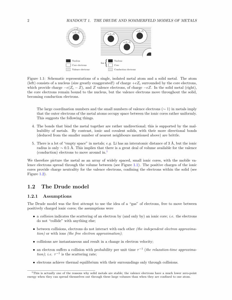
Figure 1.1: Schematic representations of a single, isolated metal atom and a solid metal. The atom(left) consists of a nucleus (size greatly exaggerated!) of charge +eZc surrounded by the core electrons,which provide charge −e(Zc − Z), and Z valence electrons, of charge −eZ. In the solid metal (right),the core electrons remain bound to the nucleus, but the valence electrons move throughout the solid,becoming conduction electrons.

The large coordination numbers and the small numbers of valence electrons (∼ 1) in metals implythat the outer electrons of the metal atoms occupy space between the ionic cores rather uniformly.This suggests the following things.

4. The bonds that bind the metal together are rather undirectional; this is supported by the mal-leability of metals. By contrast, ionic and covalent solids, with their more directional bonds(deduced from the smaller number of nearest neighbours mentioned above) are brittle.

5. There is a lot of “empty space” in metals; e.g. Li has an interatomic distance of 3 A, but the ionicradius is only ∼ 0.5 A. This implies that there is a great deal of volume available for the valence(conduction) electrons to move around in.1

We therefore picture the metal as an array of widely spaced, small ionic cores, with the mobile va-lence electrons spread through the volume between (see Figure 1.1). The positive charges of the ioniccores provide charge neutrality for the valence electrons, confining the electrons within the solid (seeFigure 1.2).

1.2 The Drude model

1.2.1 Assumptions

The Drude model was the first attempt to use the idea of a “gas” of electrons, free to move betweenpositively charged ionic cores; the assumptions were

• a collision indicates the scattering of an electron by (and only by) an ionic core; i.e. the electronsdo not “collide” with anything else;

• between collisions, electrons do not interact with each other (the independent electron approxima-tion) or with ions (the free electron approximation);

• collisions are instantaneous and result in a change in electron velocity;

• an electron suffers a collision with probability per unit time τ−1 (the relaxation-time approxima-tion); i.e. τ−1 is the scattering rate;

• electrons achieve thermal equilibrium with their surroundings only through collisions.

1This is actually one of the reasons why solid metals are stable; the valence electrons have a much lower zero-pointenergy when they can spread themselves out through these large volumes than when they are confined to one atom.

1.2. THE DRUDE MODEL 3

-1

0

(b)(a)

En

erg

y/V

0

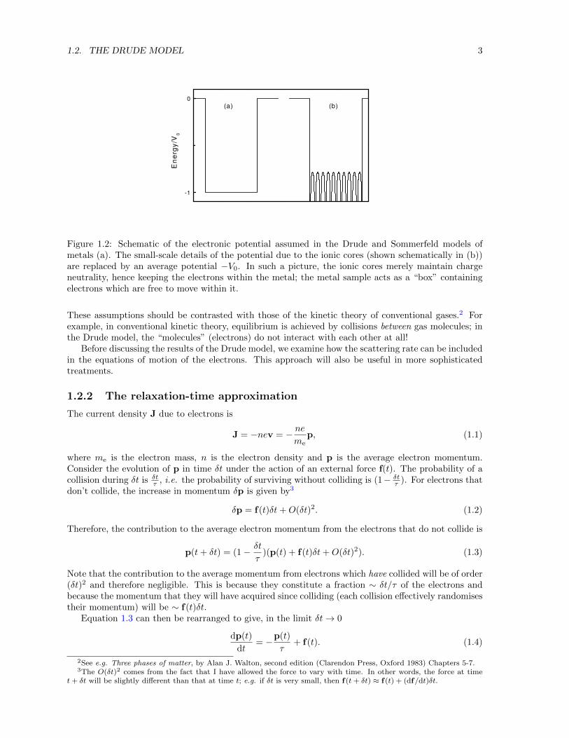
Figure 1.2: Schematic of the electronic potential assumed in the Drude and Sommerfeld models ofmetals (a). The small-scale details of the potential due to the ionic cores (shown schematically in (b))are replaced by an average potential −V0. In such a picture, the ionic cores merely maintain chargeneutrality, hence keeping the electrons within the metal; the metal sample acts as a “box” containingelectrons which are free to move within it.

These assumptions should be contrasted with those of the kinetic theory of conventional gases.2 Forexample, in conventional kinetic theory, equilibrium is achieved by collisions between gas molecules; inthe Drude model, the “molecules” (electrons) do not interact with each other at all!

Before discussing the results of the Drude model, we examine how the scattering rate can be includedin the equations of motion of the electrons. This approach will also be useful in more sophisticatedtreatments.

1.2.2 The relaxation-time approximation

The current density J due to electrons is

J = −nev = − neme

p, (1.1)

where me is the electron mass, n is the electron density and p is the average electron momentum.Consider the evolution of p in time δt under the action of an external force f(t). The probability of acollision during δt is δt

τ , i.e. the probability of surviving without colliding is (1− δtτ ). For electrons that

don’t collide, the increase in momentum δp is given by3

δp = f(t)δt+O(δt)2. (1.2)

Therefore, the contribution to the average electron momentum from the electrons that do not collide is

p(t+ δt) = (1− δt

τ)(p(t) + f(t)δt+O(δt)2). (1.3)

Note that the contribution to the average momentum from electrons which have collided will be of order(δt)2 and therefore negligible. This is because they constitute a fraction ∼ δt/τ of the electrons andbecause the momentum that they will have acquired since colliding (each collision effectively randomisestheir momentum) will be ∼ f(t)δt.

Equation 1.3 can then be rearranged to give, in the limit δt→ 0

dp(t)

dt= −p(t)

τ+ f(t). (1.4)

2See e.g. Three phases of matter, by Alan J. Walton, second edition (Clarendon Press, Oxford 1983) Chapters 5-7.3The O(δt)2 comes from the fact that I have allowed the force to vary with time. In other words, the force at time

t+ δt will be slightly different than that at time t; e.g. if δt is very small, then f(t+ δt) ≈ f(t) + (df/dt)δt.

4 HANDOUT 1. THE DRUDE AND SOMMERFELD MODELS OF METALS

In other words, the collisions produce a frictional damping term. This idea will have many applications,even beyond the Drude model; we now use it to derive the electrical conductivity.

The electrical conductivity σ is defined by

J = σE, (1.5)

where E is the electric field. To find σ, we substitute f = −eE into Equation 1.4; we also set dp(t)dt = 0,

as we are looking for a steady-state solution. The momentum can then be substituted into Equation 1.1,to give

σ = ne2τ/me. (1.6)

If we substitute the room-temperature value of σ for a typical metal4 along with a typical n ∼ 1022 −1023cm−3 into this equation, a value of τ ∼ 1− 10 fs emerges. In Drude’s picture, the electrons are theparticles of a classical gas, so that they will possess a mean kinetic energy

1

2me〈v2〉 =

3

2kBT (1.7)

(the brackets 〈 〉 denote the mean value of a quantity). Using this expression to derive a typicalclassical room temperature electron speed, we arrive at a mean free path vτ ∼ 0.1 − 1 nm. This isroughly the same as the interatomic distances in metals, a result consistent with the Drude picture ofelectrons colliding with the ionic cores. However, we shall see later that the Drude model very seriouslyunderestimates typical electronic velocities.

1.3 The failure of the Drude model

1.3.1 Electronic heat capacity

The Drude model predicts the electronic heat capacity to be the classical “equipartition of energy”result5 i.e.

Cel =3

2nkB. (1.8)

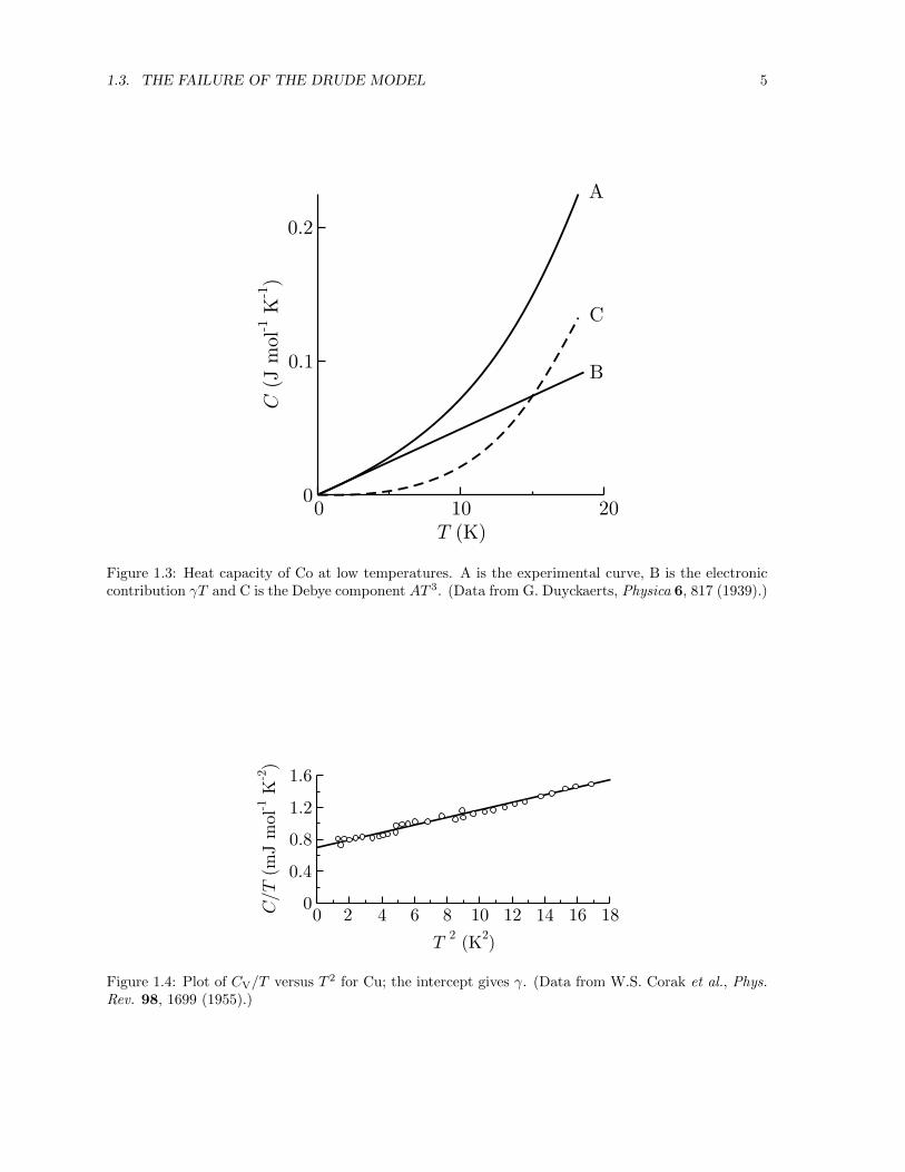
This is independent of temperature. Experimentally, the low-temperature heat capacity of metalsfollows the relationship (see Figures 1.3 and 1.4)

CV = γT +AT 3. (1.9)

The second term is obviously the phonon (Debye) component, leading us to suspect that Cel = γT .Indeed, even at room temperature, the electronic component of the heat capacity of metals is muchsmaller than the Drude prediction. This is obviously a severe failing of the model.

1.3.2 Thermal conductivity and the Wiedemann-Franz ratio

The thermal conductivity κ is defined by the equation

Jq = −κ∇T, (1.10)

where Jq is the flux of heat (i.e. energy per second per unit area). The Drude model assumes that theconduction of heat in metals is almost entirely due to electrons, and uses the kinetic theory expression6

for κ, i.e.

κ =1

3〈v2〉τCel. (1.11)

4Most metals have resistivities (1/σ) in the range ∼ 1 − 20 µΩcm at room temperature. Some typical values aretabulated on page 8 of Solid State Physics, by N.W Ashcroft and N.D. Mermin (Holt, Rinehart and Winston, New York1976).

5See any statistical mechanics book (e.g. Three phases of matter, by Alan J. Walton, second edition (Clarendon Press,Oxford 1983) page 126; Statistical Physics, by Tony Guenault (Routledge, London 1988) Section 3.2.2).

6See any kinetic theory book, e.g. Three phases of matter, by Alan J. Walton, second edition (Clarendon Press, Oxford1983) Section 7.3.

1.3. THE FAILURE OF THE DRUDE MODEL 5

0.2

0.1

00 10 20

T (K)

C(J

mol

K)

-1-1

A

C

B

Figure 1.3: Heat capacity of Co at low temperatures. A is the experimental curve, B is the electroniccontribution γT and C is the Debye component AT 3. (Data from G. Duyckaerts, Physica 6, 817 (1939).)

T2 2

(K )

CT/

(mJ m

olK

)-1

-2 1.6

1.2

0.8

0.4

00 2 4 6 8 10 12 14 1816

Figure 1.4: Plot of CV/T versus T 2 for Cu; the intercept gives γ. (Data from W.S. Corak et al., Phys.Rev. 98, 1699 (1955).)

6 HANDOUT 1. THE DRUDE AND SOMMERFELD MODELS OF METALS

1

0

L L/ 0

Impure

Ideallypure

Temperature

Figure 1.5: Schematic of experimental variation of L = κ/(σT ) with temperature; L0 is the theoret-ical value of L derived in later lectures. The high temperature limit of the figure represents roomtemperature.

Cel is taken from Equation 1.8 and the speed takes the classical thermal value, i.e. 12me〈v2〉 = 3

2kBT .The fortuitous success of this approach came with the prediction of the Wiedemann-Franz ratio,

κ/σ. It had been found that the Wiedemann-Franz ratio divided by the temperature, L = κ/(σT ),7 wasclose to the constant value ∼ 2.5× 10−8WΩK−2 for many metals at room temperature.8 SubstitutingEquations 1.6 and 1.11 into this ratio leads to

κ

σT=

3

2

k2B

e2≈ 1.1× 10−8WΩK−2. (1.12)

However, in spite of this apparent success, the individual components of the model are very wrong; e.g.Cel in the Drude model is at least two orders of magnitude bigger than the experimental values at roomtemperature! Furthermore, experimentally κ/(σT ) drops away from its constant value at temperaturesbelow room temperature (see Figure 1.5); the Drude model cannot explain this behaviour.

1.3.3 Hall effect

The Hall effect occurs when a magnetic field B is applied perpendicular to a current density J flowingin a sample. A Hall voltage is developed in the direction perpendicular to both J and B. We assumethat the current flows parallel to the x direction and that B is parallel to to z direction; the Hall voltagewill then be developed in the y direction.

The presence of both electric and magnetic fields means that the force on an electron is now f =−eE− ev ×B. Equation 1.4 becomes

dv

dt= − e

meE− e

mev ×B− v

τ. (1.13)

In steady state, the left-hand side vanishes, and the two components of the equation read

vx = − eτme

Ex − ωcτvy (1.14)

andvy = − eτ

meEy + ωcτvx, (1.15)

where we have written ωc = eB/me (ωc is of course the classical cyclotron angular frequency). If weimpose the condition vy = 0 (no current in the y direction) we have

EyEx

= −ωcτ. (1.16)

7L = κ/(σT ) is often referred to as the Lorenz number.8Typical values of κ and σ for metals are available in Tables of Physical and Chemical Constants, by G.W.C. Kaye

and T.H. Laby (Longmans, London, 1966); find the book and check out the Lorenz number for yourself!

1.4. THE SOMMERFELD MODEL 7

0.01 0.1 1.0 10 100 1000

-0.33

-1/R neH

w t tc

= eB /me

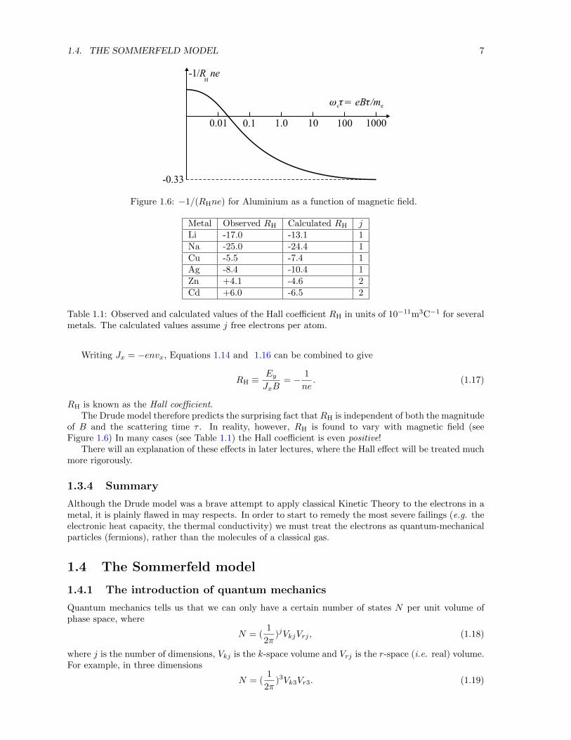
Figure 1.6: −1/(RHne) for Aluminium as a function of magnetic field.

Metal Observed RH Calculated RH jLi -17.0 -13.1 1Na -25.0 -24.4 1Cu -5.5 -7.4 1Ag -8.4 -10.4 1Zn +4.1 -4.6 2Cd +6.0 -6.5 2

Table 1.1: Observed and calculated values of the Hall coefficient RH in units of 10−11m3C−1 for severalmetals. The calculated values assume j free electrons per atom.

Writing Jx = −envx, Equations 1.14 and 1.16 can be combined to give

RH ≡EyJxB

= − 1

ne. (1.17)

RH is known as the Hall coefficient.The Drude model therefore predicts the surprising fact that RH is independent of both the magnitude

of B and the scattering time τ . In reality, however, RH is found to vary with magnetic field (seeFigure 1.6) In many cases (see Table 1.1) the Hall coefficient is even positive!

There will an explanation of these effects in later lectures, where the Hall effect will be treated muchmore rigorously.

1.3.4 Summary

Although the Drude model was a brave attempt to apply classical Kinetic Theory to the electrons in ametal, it is plainly flawed in may respects. In order to start to remedy the most severe failings (e.g. theelectronic heat capacity, the thermal conductivity) we must treat the electrons as quantum-mechanicalparticles (fermions), rather than the molecules of a classical gas.

1.4 The Sommerfeld model

1.4.1 The introduction of quantum mechanics

Quantum mechanics tells us that we can only have a certain number of states N per unit volume ofphase space, where

N = (1

2π)jVkjVrj , (1.18)

where j is the number of dimensions, Vkj is the k-space volume and Vrj is the r-space (i.e. real) volume.For example, in three dimensions

N = (1

2π)3Vk3Vr3. (1.19)

8 HANDOUT 1. THE DRUDE AND SOMMERFELD MODELS OF METALS

Now we assume electrons free to move within the solid; once again we ignore the details of theperiodic potential due to the ionic cores (see Figure 1.2(b)),9 replacing it with a mean potential −V0

(see Figure 1.2(a)). The energy of the electrons is then

E(k) = −V0 +p2

2me= −V0 +

h2k2

2me. (1.20)

However, we are at liberty to set the origin of energy; for convenience we choose E = 0 to correspondto the average potential within the metal (Figure 1.2(a)), so that

E(k) =h2k2

2me. (1.21)

Let us now imagine gradually putting free electrons into a metal. At T = 0, the first electrons willoccupy the lowest energy (i.e. lowest |k|) states; subsequent electrons will be forced to occupy higherand higher energy states (because of Pauli’s Exclusion Principle). Eventually, when all N electrons areaccommodated, we will have filled a sphere of k-space, with

N = 2(1

2π)3 4

3πk3

FVr3, (1.22)

where we have included a factor 2 to cope with the electrons’ spin degeneracy and where kF is thek-space radius (the Fermi wavevector) of the sphere of filled states. Rearranging, remembering thatn = N/Vr3, gives

kF = (3π2n)13 . (1.23)

The corresponding electron energy is

EF =h2k2

F

2me=

h2

2me(3π2n)

23 . (1.24)

This energy is called the Fermi energy.The substitution of typical metallic carrier densities into Equation 1.24,10 produces values of EF

in the range ∼ 1.5 − 15 eV (i.e. ∼ atomic energies) or EF/kB ∼ 20 − 100 × 103 K (i.e. roomtemperature). Typical Fermi wavevectors are kF ∼ 1/(the atomic spacing) ∼ the Brillouin zone size∼ typical X-ray k-vectors. The velocities of electrons at the Fermi surface are vF = hkF/me ∼ 0.01c.Although the Fermi surface is the T = 0 groundstate of the electron system, the electrons present areenormously energetic!

The presence of the Fermi surface has many consequences for the properties of metals; e.g. the maincontribution to the bulk modulus of metals comes from the Fermi “gas” of electrons.11

1.4.2 The Fermi-Dirac distribution function.

In order to treat the thermal properties of electrons at higher temperatures, we need an appropriatedistribution function for electrons from Statistical Mechanics. The Fermi-Dirac distribution function is

fD(E, T ) =1

e(E−µ)/kBT + 1, (1.25)

9Many condensed matter physics texts spend time on hand-waving arguments which supposedly justify the fact thatelectrons do not interact much with the ionic cores. Justifications used include “the ionic cores are very small”; “theelectron–ion interactions are strongest at small separations but the Pauli exclusion principle prevents electrons fromentering this region”; “screening of ionic charge by the mobile valence electrons”; “electrons have higher average kineticenergies whilst traversing the deep ionic potential wells and therefore spend less time there”. We shall see in later lecturesthat it is the translational symmetry of the potential due to the ions which allows the electrons to travel for long distanceswithout scattering from anything.

10Metallic carrier densities are usually in the range ∼ 1022 − 1023cm−3. Values for several metals are tabulated inSolid State Physics, by N.W Ashcroft and N.D. Mermin (Holt, Rinehart and Winston, New York 1976), page 5. See alsoProblem 1.

11See Problem 2; selected bulk moduli for metals have been tabulated on page 39 of Solid State Physics, by N.WAshcroft and N.D. Mermin (Holt, Rinehart and Winston, New York 1976).

1.4. THE SOMMERFELD MODEL 9

f

f

1.0

1.0

(a)

(b)

¹

¹

²

²

(¢ )E k T¼ B

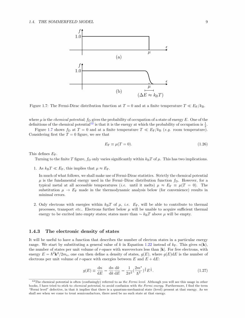
Figure 1.7: The Fermi-Dirac distribution function at T = 0 and at a finite temperature T EF/kB.

where µ is the chemical potential; fD gives the probability of occupation of a state of energy E. One of thedefinitions of the chemical potential12 is that it is the energy at which the probability of occupation is 1

2 .

Figure 1.7 shows fD at T = 0 and at a finite temperature T EF/kB (e.g. room temperature).Considering first the T = 0 figure, we see that

EF ≡ µ(T = 0). (1.26)

This defines EF.

Turning to the finite T figure, fD only varies significantly within kBT of µ. This has two implications.

1. As kBT EF, this implies that µ ≈ EF.

In much of what follows, we shall make use of Fermi-Dirac statistics. Strictly the chemical potentialµ is the fundamental energy used in the Fermi–Dirac distribution function fD. However, for atypical metal at all accessible temperatures (i.e. until it melts) µ ≈ EF ≡ µ(T = 0). Thesubstitution µ → EF made in the thermodynamic analysis below (for convenience) results inminimal errors.

2. Only electrons with energies within kBT of µ, i.e. EF, will be able to contribute to thermalprocesses, transport etc.. Electrons further below µ will be unable to acquire sufficient thermalenergy to be excited into empty states; states more than ∼ kBT above µ will be empty.

1.4.3 The electronic density of states

It will be useful to have a function that describes the number of electron states in a particular energyrange. We start by substituting a general value of k in Equation 1.22 instead of kF. This gives n(k),the number of states per unit volume of r-space with wavevectors less than |k|. For free electrons, withenergy E = h2k2/2me, one can then define a density of states, g(E), where g(E)dE is the number ofelectrons per unit volume of r-space with energies between E and E + dE:

g(E) ≡ dn

dE=

dn

dk

dk

dE=

1

2π2(2m∗

h2 )32E

12 . (1.27)

12The chemical potential is often (confusingly) referred to as the Fermi level. Although you will see this usage in otherbooks, I have tried to stick to chemical potential, to avoid confusion with the Fermi energy. Furthermore, I find the term“Fermi level” defective, in that it implies that there is a quantum-mechanical state (level) present at that energy. As weshall see when we come to treat semiconductors, there need be no such state at that energy.

10 HANDOUT 1. THE DRUDE AND SOMMERFELD MODELS OF METALS

0.2

0.4

0.6

0.8

1.0

2000

10 30 40 50 60 70 80 90 100 110

fMB

f

f

fMB

fFD

x mv k T= /22

B

x mv k T= /22

B

0 1 2 3 4 5 6 7 8 9

100

200

300

400

500

600

700

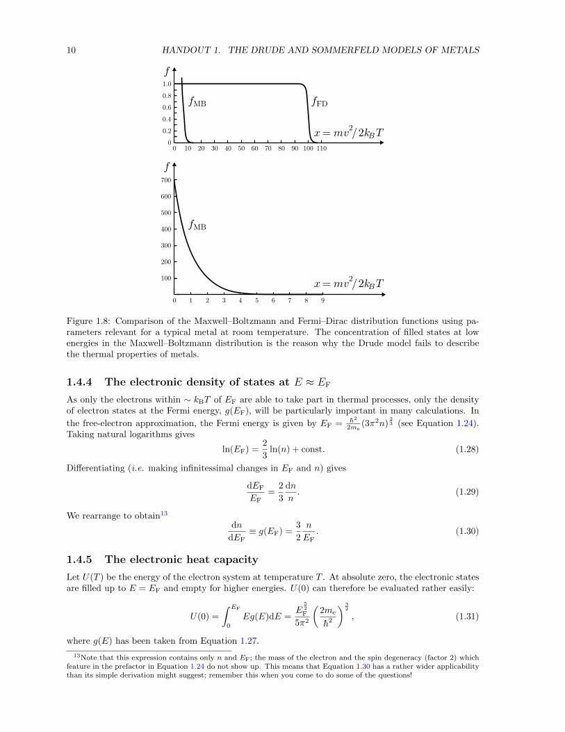
Figure 1.8: Comparison of the Maxwell–Boltzmann and Fermi–Dirac distribution functions using pa-rameters relevant for a typical metal at room temperature. The concentration of filled states at lowenergies in the Maxwell–Boltzmann distribution is the reason why the Drude model fails to describethe thermal properties of metals.

1.4.4 The electronic density of states at E ≈ EF

As only the electrons within ∼ kBT of EF are able to take part in thermal processes, only the densityof electron states at the Fermi energy, g(EF), will be particularly important in many calculations. In

the free-electron approximation, the Fermi energy is given by EF = h2

2me(3π2n)

23 (see Equation 1.24).

Taking natural logarithms gives

ln(EF) =2

3ln(n) + const. (1.28)

Differentiating (i.e. making infinitessimal changes in EF and n) gives

dEF

EF=

2

3

dn

n. (1.29)

We rearrange to obtain13

dn

dEF≡ g(EF) =

3

2

n

EF. (1.30)

1.4.5 The electronic heat capacity

Let U(T ) be the energy of the electron system at temperature T . At absolute zero, the electronic statesare filled up to E = EF and empty for higher energies. U(0) can therefore be evaluated rather easily:

U(0) =

∫ EF

0

Eg(E)dE =E

52

F

5π2

(2me

h2

) 32

, (1.31)

where g(E) has been taken from Equation 1.27.

13Note that this expression contains only n and EF; the mass of the electron and the spin degeneracy (factor 2) whichfeature in the prefactor in Equation 1.24 do not show up. This means that Equation 1.30 has a rather wider applicabilitythan its simple derivation might suggest; remember this when you come to do some of the questions!

1.4. THE SOMMERFELD MODEL 11

At finite temperature, electrons are excited into higher levels, and the expression for the energy ofthe electron system becomes slightly more complicated

U(T ) =

∫ ∞0

E g(E) fD(E, T )dE

=1

2π2

(2me

h2

) 32∫ ∞

0

E32

(e(E−µ)/kBT + 1)dE. (1.32)

The integral in Equation 1.32 is a member of the family of so-called Fermi–Dirac integrals

Fj(y0) =

∫ ∞0

yj

e(y−y0) + 1dy. (1.33)

There are no general analytical expressions for such integrals, but certain asymptotic forms exist. Com-parison with Equation 1.32 shows that y0 ≡ µ/kBT ; we have seen that for all practical temperatures,µ ≈ EF kBT . Hence, the asymptotic form that is of interest for us is the one for y0 very large andpositive:

Fj(y0) ≈ yj+10

j + 1

(1 +

π2j(j + 1)

6y20

+O(y−40 ) + ...

)(1.34)

Using Equation 1.34 to evaluate Equation 1.32 in the limit µ kBT yields

U(T ) =2

5µ

52 1 +

5

8

(πkBT

µ

)2

1

2π2

(2me

h2

) 32

. (1.35)

We are left with the problem that µ is temperature dependent; µ is determined by the constraint thatthe total number of electrons must remain constant:

n =

∫ ∞0

g(E) fD(E, T )dE

=1

2π2

(2me

h2

) 32∫ ∞

0

E12

(e(E−µ)/kBT + 1)dE. (1.36)

This contains the j = 12 Fermi–Dirac integral, which may also be evaluated using Equation 1.34 (as

µ kBT ) to yield

µ ≈ EF1−π2

12

(kBT

µ

)2

. (1.37)

Therefore, using a polynomial expansion

µ52 ≈ E

52

F 1−5π2

24

(kBT

µ

)2

....., (1.38)

Combining Equations 1.35 and 1.38 and neglecting terms of order (kBT/EF)4 gives

U(T ) ≈ 2

5E

52

F 1−5π2

24

(kBT

µ

)2

1 +5

8

(πkBT

µ

)2

1

2π2

(2me

h2

) 32

.

≈ 2

5E

52

F 1 +5

12

(πkBT

µ

)2

1

2π2

(2me

h2

) 32

. (1.39)

Thus far, it was essential to keep the temperature dependence of µ in the algebra in order to getthe prefactor of the temperature-dependent term in Equation 1.39 correct. However, Equation 1.37shows that at temperatures kBT µ (e.g. at room temperature in typical metal), µ ≈ EF to a highdegree of accuracy. In order to get a reasonably accurate estimate for U(T ) we can therefore make thesubstitution µ→ EF in denominator of the second term of the bracket of Equation 1.39 to give

U(T ) = U(0) +nπ2k2

BT2

4EF, (1.40)

12 HANDOUT 1. THE DRUDE AND SOMMERFELD MODELS OF METALS

where we have substituted in the value for U(0) from Equation 1.31. Differentiating, we obtain

Cel ≡∂U

∂T=

1

2π2n

k2BT

EF. (1.41)

Equation 1.41 looks very good as it

1. is proportional to T , as are experimental data (see Figures 1.3 and 1.4);

2. is a factor ∼ kBTEF

smaller than the classical (Drude) value, as are experimental data.

Just in case the algebra of this section has seemed like hard work,14 note that a reasonably accurateestimate of Cel can be obtained using the following reasoning. At all practical temperatures, kBT EF,so that we can say that only the electrons in an energy range ∼ kBT on either side of µ ≈ EF willbe involved in thermal processes. The number density of these electrons will be ∼ kBTg(EF). Eachelectron will be excited to a state ∼ kBT above its groundstate (T = 0) energy. A reasonable estimateof the thermal energy of the system will therefore be

U(T )− U(0) ∼ (kBT )2g(EF) =3

2nkBT

(kBT

EF

),

where I have substituted the value of g(EF) from Equation 1.30. Differentiating with respect to T , weobtain

Cel = 3nkB

(kBT

EF

),

which is within a factor 2 of the more accurate method.

1.5 Successes and failures of the Sommerfeld model

The Sommerfeld model is a great improvement on the Drude model; it can successfully explain

• the temperature dependence and magnitude of Cel;

• the approximate temperature dependence and magnitudes of the thermal and electrical conduc-tivities of metals, and the Wiedemann–Franz ratio (see later lectures);

• the fact that the electronic magnetic susceptibility is temperature independent.15

It cannot explain

• the Hall coefficients of many metals (see Figure 1.6 and Table 1.1; Sommerfeld predicts RH =−1/ne);

• the magnetoresistance exhibited by metals (see subsequent lectures);

• other parameters such as the thermopower;

• the shapes of the Fermi surfaces in many real metals;

• the fact that some materials are insulators and semiconductors (i.e. not metals).

Furthermore, it seems very intellectually unsatisfying to completely disregard the interactions betweenthe electrons and the ionic cores, except as a source of instantaneous “collisions”. This is actuallythe underlying source of the difficulty; to remedy the failures of the Sommerfeld model, we must re-introduce the interactions between the ionic cores and the electrons. In other words, we must introducethe periodic potential of the lattice.

14The method for deriving the electronic heat capacity used in books such as Introduction to Solid State Physics,by Charles Kittel, seventh edition (Wiley, New York 1996) looks at first sight rather simpler than the one that I havefollowed. However, Kittel’s method contains a hidden trap which is not mentioned; it ignores (dµ/dT ), which is said tobe negligible. This term is actually of comparable size to all of the others in Kittel’s integral (see Solid State Physics, byN.W Ashcroft and N.D. Mermin (Holt, Rinehart and Winston, New York 1976) Chapter 2), but happens to disappearbecause of a cunning change of variables. By the time all of this has explained in depth, Kittel’s method looks rathermore tedious and less clear, and I do not blame him for wishing to gloss over the point!

15The susceptibility of metals in the Sommerfeld model is derived in Chapter 7 of Magnetism in Condensed Matter, byS.J. Blundell (OUP 2000).

1.6. READING. 13

1.6 Reading.

A more detailed treatment of the topics in this Chapter is given in Solid State Physics, by N.W Ashcroftand N.D. Mermin (Holt, Rinehart and Winston, New York 1976) Chapters 1-3 and Band theory andelectronic properties of solids, by John Singleton (Oxford University Press, 2001) Chapter 1. Otheruseful information can be found in Electricity and Magnetism, by B.I. Bleaney and B. Bleaney, revisedthird/fourth editions (Oxford University Press, Oxford) Chapter 11, Solid State Physics, by G. Burns(Academic Press, Boston, 1995) Sections 9.1-9.14, Electrons in Metals and Semiconductors, by R.G.Chambers (Chapman and Hall, London 1990) Chapters 1 and 2, and Introduction to Solid State Physics,by Charles Kittel, seventh edition (Wiley, New York 1996) Chapters 6 and 7.