The dose delivery monitor of the rst LINAC for ... · LINAC for protontherapy: test, calibration...
114
FACOLT ` A DI SCIENZE MATEMATICHE FISICHE E NATURALI Corso di Laurea Magistrale in Fisica The dose delivery monitor of the first LINAC for protontherapy: test, calibration and beam characterization Relatore Interno: Prof. Riccardo Faccini Candidata: Cristina Placido Relatore Esterno: Dott. Evaristo Cisbani Matricola: 1423908 Sessione autunnale Anno Accademico 2015/2016 Dipartimento di Fisica
Transcript of The dose delivery monitor of the rst LINAC for ... · LINAC for protontherapy: test, calibration...

FACOLTA DI SCIENZE MATEMATICHE FISICHE E NATURALI
Corso di Laurea Magistrale in Fisica
The dose delivery monitor of the firstLINAC for protontherapy: test, calibration
and beam characterization
Relatore Interno:
Prof. Riccardo Faccini
Candidata:
Cristina Placido
Relatore Esterno:
Dott. Evaristo Cisbani
Matricola:
1423908
Sessione autunnale
Anno Accademico 2015/2016
Dipartimento di Fisica

Abstract
Use of accelerated protons or heavier ions is gaining more and more relevance in
cancer therapy. Respect to the conventional radiotherapy, hadrontherapy offers an
excellent local control of deep-sited tumors or tumor close to vital organs. In fact,
hadrontherapy exploits the peculiar hadron property to release the largest amount of
dose at the end of its path in the tissue and, at the same time, small lateral spreading.
This accuracy results in a more effective irradiation of the tumour, thereby minimizing
the dose to the surrounding healthy tissues and thus reducing the side effects. However
hadrontherapy facilities construction and their operation costs are large compared to
the other cancer therapies and this represents a serious drawback for its diffusion.
The innovative TOP-IMPLART project, developed by the collaboration between ENEA,
IFO and ISS, moves in the direction of highest therapeutic impact and at the same time
costs reduction by the exploitation, for the first time in cancer therapy, of a dedicated
LINAC proton accelerator. The high ballistic precision of protons and, in turn, the
better conformation of the dose delivery achievable by the TOP-IMPLART system,
require an equally accurate control of the beam parameters and of the dose released
to the patient on a pulse by pulse basis. In this regard, as part of the TOP-IMPLART
project, a dedicated dose delivery monitor is under developement. The device consists
in a set of ionization chambers using Micro Pattern Gaseous Detector (MPGD) tech-
nology, coupled to electronics with dynamic variation of the single channel gain. Each
chamber shall provide real-time measurements of the X and Y beam intensity profiles,
beam centroid position and its direction, in order to guarantee that the prescribed
dose is optimally delivered. The first prototype has been characterized and tested on
the TOP-IMPLART proton beam at the current energy of 27 MeV.
The aim of this thesis is to introduce the principles of operation of the dose deliv-
ery monitoring system and to present its first characterization, tests of operation and
preliminary dose calibration with the 27 MeV TOP-IMPLART beam.
The first Chapter introduces the hadrontherapy: the physics and radiobiological prin-
ciples and processes are presented after an overview of the main radiation therapy
i

features. The main technological components of the hadrontherapy facilities are de-
scribed in the second Chapter. In Chapter 3 the TOP-IMPLART system is introduced
providing a brief description of the accelerator features and a more accurate description
of the monitoring system. Finally the last Chapter summarizes, with some details, the
results obtained by the first tests of the monitor and its preliminary dose calibration,
which represent the original work of this thesis.
As part of the TOP-IMPLART project, the activities that I have done for my thesis
work mainly concern the partecipation to the hardware development of the dose deliv-
ery system and of the integral chamber used as a reference monitor, the contribution
to the properly measure plans definitions, carrying out measures and the subsequent
data analysis, comparing the results with dosimetrists and trying to understand the
obtained results.
ii

Contents
Abstract i
1 Principles of hadrontherapy and related physics 2
1.1 Introduction . . . . . . . . . . . . . . . . . . . . . . . . . . . . . . . . . . 2
1.2 General features of radiation therapy . . . . . . . . . . . . . . . . . . . . 4
1.2.1 Absorbed Dose . . . . . . . . . . . . . . . . . . . . . . . . . . . . 4
1.2.2 Conventional Radiotherapy . . . . . . . . . . . . . . . . . . . . . 5
1.2.3 Hadrontherapy . . . . . . . . . . . . . . . . . . . . . . . . . . . . 6
1.2.3.1 Historical background and current status of hadron-
therapy . . . . . . . . . . . . . . . . . . . . . . . . . . . 7
1.3 Physics of charged hadrons . . . . . . . . . . . . . . . . . . . . . . . . . 11
1.3.1 Electromagnetic interactions . . . . . . . . . . . . . . . . . . . . 11
1.3.2 Nuclear interactions . . . . . . . . . . . . . . . . . . . . . . . . . 13
1.3.3 Range . . . . . . . . . . . . . . . . . . . . . . . . . . . . . . . . . 15
1.3.4 Linear Energy Transfer . . . . . . . . . . . . . . . . . . . . . . . 17
1.3.5 Bragg curve . . . . . . . . . . . . . . . . . . . . . . . . . . . . . . 19
1.4 Radiobiological properties of hadrons . . . . . . . . . . . . . . . . . . . . 22
1.4.1 Radiation damage to DNA . . . . . . . . . . . . . . . . . . . . . 22
1.4.2 Relative Biological Effectiveness . . . . . . . . . . . . . . . . . . 24
1.4.3 Oxigen Enhancement Ratio . . . . . . . . . . . . . . . . . . . . . 26
2 Equipment for hadrontherapy facilities 28
2.1 Accelerator systems for hadrontherapy . . . . . . . . . . . . . . . . . . . 28
2.1.1 Cyclotron . . . . . . . . . . . . . . . . . . . . . . . . . . . . . . . 30
2.1.2 Synchrotron . . . . . . . . . . . . . . . . . . . . . . . . . . . . . . 32
2.1.3 Linear Accelerators . . . . . . . . . . . . . . . . . . . . . . . . . . 33
2.1.3.1 Advantages and disadvantages of proton-LINAC . . . . 33
2.2 Dose delivery systems . . . . . . . . . . . . . . . . . . . . . . . . . . . . 34
2.2.1 Passive beam delivery system . . . . . . . . . . . . . . . . . . . . 34
iii
CONTENTS
2.2.2 Active beam delivery system . . . . . . . . . . . . . . . . . . . . 35
2.3 Dose delivery monitor . . . . . . . . . . . . . . . . . . . . . . . . . . . . 36
2.3.1 Radiation detector for medical applications . . . . . . . . . . . . 38
2.3.1.1 Ionization chamber . . . . . . . . . . . . . . . . . . . . 38
2.3.1.2 Secondary emission monitors (SEMS) . . . . . . . . . . 42
2.3.1.3 Multi wire proportional chamber . . . . . . . . . . . . . 43
2.3.1.4 Calorimeters . . . . . . . . . . . . . . . . . . . . . . . . 43
2.3.1.5 Semiconductor detectors . . . . . . . . . . . . . . . . . 43
2.3.1.6 Scintillators . . . . . . . . . . . . . . . . . . . . . . . . . 44
2.3.1.7 Dosimetric films . . . . . . . . . . . . . . . . . . . . . . 44
2.3.1.8 Alanine detectors . . . . . . . . . . . . . . . . . . . . . 45
2.3.1.9 Faraday cups . . . . . . . . . . . . . . . . . . . . . . . . 45
3 The TOP-IMPLART system 47
3.1 The TOP accelerator . . . . . . . . . . . . . . . . . . . . . . . . . . . . . 48
3.2 Beam monitoring . . . . . . . . . . . . . . . . . . . . . . . . . . . . . . . 51
3.2.1 The Pad-Strip Ionization chamber and its prototype . . . . . . . 52
3.2.2 The readout electronics . . . . . . . . . . . . . . . . . . . . . . . 53
3.2.2.1 Input stage and adaptive gain change . . . . . . . . . . 55
4 Test and Calibration of the monitor chamber 60
4.1 Experimental setup . . . . . . . . . . . . . . . . . . . . . . . . . . . . . . 60
4.2 Preliminary considerations . . . . . . . . . . . . . . . . . . . . . . . . . . 62
4.3 Ionization regime . . . . . . . . . . . . . . . . . . . . . . . . . . . . . . . 63
4.4 Tests of operation . . . . . . . . . . . . . . . . . . . . . . . . . . . . . . 64
4.4.1 Pedestal . . . . . . . . . . . . . . . . . . . . . . . . . . . . . . . . 64
4.4.2 Channels equalization procedure . . . . . . . . . . . . . . . . . . 67
4.4.3 X/Y charge collection . . . . . . . . . . . . . . . . . . . . . . . . 70
4.5 Automatic gain change . . . . . . . . . . . . . . . . . . . . . . . . . . . . 72
4.5.1 Gain calibration . . . . . . . . . . . . . . . . . . . . . . . . . . . 72
4.5.1.1 Method 1: Channels with gain change oscillating dur-
ing the run . . . . . . . . . . . . . . . . . . . . . . . . . 75
4.5.1.2 Method 2: Channels undergoing gain change in the
entire run . . . . . . . . . . . . . . . . . . . . . . . . . . 75
4.6 Dose measurements . . . . . . . . . . . . . . . . . . . . . . . . . . . . . . 77
4.6.1 Dose comparison . . . . . . . . . . . . . . . . . . . . . . . . . . . 81
4.6.1.1 Calibration with GaFchromic films . . . . . . . . . . . . 82
4.6.1.2 Calibration with Alanine pills . . . . . . . . . . . . . . 87
iv

CONTENTS
4.7 Preliminary beam characterization . . . . . . . . . . . . . . . . . . . . . 89
5 Conclusions 93
Appendix 94
Addendum: further dose measurements and intercomparison 96
Bibliography 104
1

Chapter 1
Principles of hadrontherapy
and related physics
1.1 Introduction
Cancer can broadly be defined as the uncontrolled growth and proliferation of group
of cells. The transformation of healthy cells into cancerous ones is the consequence of
an alteration of genetic code which regulates the normal activities of cells.
In the developed countries about 30% of people suffer of cancer and about half of these
die from this disease [2].
Nowadays cancer is treated by several approaches, that include and quite often combine
one of the following:
Surgery;
Chemotherapy;
Immunotherapy;
Radiation therapy.
The choice of the proper therapy depends on the type of cancer, location and stage
of the disease, as well as the general state of the patient. The complete removal of
the cancer without damage to the rest of the body and limitation of side effects is
the goal of any treatment. Sometimes this can be accomplished by surgery, but in
many cases, cancers tend to invade adjacent tissues or to spread even to distant sites
by metastasis, often limiting the surgery treatment effectiveness. The effectiveness of
chemotherapy is often limited by toxicity to other tissues in the body. Radiation can
2
1. Principles of hadrontherapy and related physics
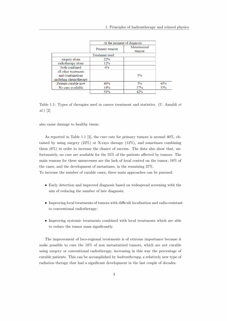
Table 1.1: Types of therapies used in cancer treatment and statistics. (U. Amaldi et
al.) [2]
also cause damage to healthy tissue.
As reported in Table 1.1 [2], the cure rate for primary tumors is around 40%, ob-
tained by using surgery (22%) or X-rays therapy (12%), and sometimes combining
them (6%) in order to increase the chance of success. The data also show that, un-
fortunately, no cure are available for the 55% of the patients affected by tumors. The
main reasons for these unsuccesses are the lack of local control on the tumor, 18% of
the cases, and the development of metastases, in the remaining 37%.
To increase the number of curable cases, three main approaches can be pursued:
Early detection and improved diagnosis based on widespread screening with the
aim of reducing the number of late diagnosis;
Improving local treatments of tumors with difficult localization and radio-resistant
to conventional radiotherapy;
Improving systemic treatments combined with local treatments which are able
to reduce the tumor mass significantly.
The improvement of loco-regional treatments is of extreme importance because it
make possible to cure the 18% of non metastatized tumors, which are not curable
using surgery or conventional radiotherapy, increasing in this way the percentage of
curable patients. This can be accomplished by hadrontherapy, a relatively new type of
radiation therapy that had a significant development in the last couple of decades.
3

1. Principles of hadrontherapy and related physics
1.2 General features of radiation therapy
Radiation therapy, also called radiotherapy, constitues an essential component of
cancer therapy. It consists in the use of ionizing radiation (electrons, X-rays, γ-rays,
hadrons, etc...) to destroy cancer cells which, in physical terms, are considered the
targets. It can be administered both externally, via external beam radiotherapy, or
internally, via brachytherapy.
The main goal of radiation therapy is to kill as many tumoral cells as possible, in the
area being treated, by damaging their genetic material, so making them impossible to
continue to grow and/or reproduce. But, at the same time, it is necessary to control
the quantity of administered radiation and the modalities of irradiation to preserve
the surrounding healthy tissues. Hence, it is given in many fractions, allowing healthy
tissues to recover between one fraction to another.
Radiation therapy may be used to treat many types of solid tumor, including cancers
of the brain, breast, cervix, larynx, lung, pancreas, prostate, skin, stomach, uterus, or
soft tissue sarcomas. Radiation is also used to treat leukemia and lymphoma. The
amount of radiation that has to be administered to each tumoral site depends on a
number of factors, including the radiosensitivity of each cancer type and whether there
are tissues and organs nearby that may be seriously damaged by radiation.
1.2.1 Absorbed Dose
To reach the goal of any radiotherapy treatment high energy particle beams are
used. Each of these particles, penetrating in the human body, makes interactions
with the tissues. Depending on the type of particle, its charge and energy, several
interactions may occur and, in each of one an amount of energy is trasfered from the
projectile particle to the target tissue. In many cases a great amount of energy can
be released in tissues and consequently may cause the ionization of atomic species in
the interested region. This ionization events constitute the principal cause of damages
to cells, and if they are very close in space, they can produce the double strand break
of the Deoxyribonucleic acid molecule (DNA), causing the fail of any cell reparation
mechanisms and the death of the tumoral cells.
To quantify the amount of energy released by radiation, the concept of dose, has
been introduced. The absorbed dose D is defined as the ratio between the energy ED
realeased by radiation in a small volume of matter and the mass m of that volume.
In SI the ratio D = ED/m is measured in Gray (Gy), and one Gray is equal to an
absorbed energy of one Joule in one kilogram of matter.
Absorbed dose is a quantity defined for both indirectly and directly ionizing radia-
4

1. Principles of hadrontherapy and related physics
tions. For indirectly ionizing radiations, energy is imparted to matter in a two step
process: in the first step, the indirectly ionizing radiation transfers kinetic energy to
secondary charged particles; in the second step, these charged particles transfer some
of their kinetic energy to the medium (resulting in absorbed dose) and they lose some
of their energy in the form of radiative losses which do not contribute to absorbed dose.
1.2.2 Conventional Radiotherapy
The term conventional radiotherapy refers to the type of radiation therapy that
uses X-rays electrons (or γ-rays from collimated electron beams) as form of radiation.
It has been routinely used in the cure of cancer disease since the seventies.
In general electron beam energies vary in the range between 3 and 25 MeV.
The main drawback of this treatment is due to the ballistic properties of the elec-
trons and X-rays at these energies. When they traverse matter, the maximum of their
energy deposition is located at a small penetration depth, only few centimetres be-
yond the skin surface, then the realeased energy decreases slowly with respect to the
distance, in a nearly exponential way (Figure 1.1). For electrons the maximum pene-
tration depth, expressed in centimetres, is almost equal to half the initial energy of the
beam, expressed in MeV. Due to these characteristics, electron beams are suitable for
the treatment of superficial or semi-deep seated tumors at a few centimetres, starting
from the skin surface. In this way, it is difficult to accurately irradiate tumors deeply
located in the body and, at the same time, preserving the surrounding healthy tissues.
In a typical treatment one delivers in each treatment session 2-2.5 Gy to the tumour,
while giving less than 1-1.2 Gy to any of the organ at risk. Since the treatment lasts
about 30 sessions, usually spread over 6 weeks, the target will have eventually received
60-75 Gy. The cost of such an average treatment is around 3000 euros.
In order to improve the radiation therapy efficiency, several irradiation tecniques have
been developed during the last decades. The most common in use today is the In-
tensity Modulated Radio Therapy (IMRT). It is an advanced mode of high-precision
conventional radiotherapy that uses computer-controlled linear accelerators to deliver
precise radiation doses in specific areas within the tumor. IMRT, mainly consists in
a single radiation beam delivered to the patient from several directions. In this way
allows higher radiation doses to overlap in the region of the tumor (Figure 1.2) while
minimizing the dose to surrounding critical structures. Also, the use of multi-leaf
collimators allows to conform more precisely to the three-dimensional shape of the
tumor[1]. An advanced type of IMRT is represented by tomotherapy, which permits to
adjust in real time intensity and direction of the X-ray beam, to better conform it to
5

1. Principles of hadrontherapy and related physics
Figure 1.1: Dose realeased in matter by electrons of various energies as a function of
the traversed depth.
the target position and shape. CyberKnife represents a robotic radiosurgery system:
it consist in a compact low energy linac mounted on a robotic arm which allows to
use different beam incidences in 3D and hence concentrate the delivered dose on the
tumor while spreading the dose on healthy tissues.
Today the X-rays therapy is used as reference to evaluate the effectiveness of other
particle therapies.
1.2.3 Hadrontherapy
Hadrontherapy is an alternative way for the treatment of cancer. It consists in
irradiating tumors with hadrons, like protons (protontherapy), neutrons or light nuclei
(alpha particles, helium ions, carbon ions, ect...). Among all these possibilities, only
two of them, protons and carbon ions, are nowadays widely used in clinical hadron-
therapy practice.
Compared to conventional radiotherapy, hadrontherapy presents two main advantages:
At macroscopic scale: precise ballistics, with a finite and tunable range and a
maximum dose deposition at the end of the path (Bragg peak); the longitudinal
position of the peak is strongly correlated to the initial particles energy.
At microscopic scale: for particles havier than protons, enhanced biological ef-
6
1. Principles of hadrontherapy and related physics
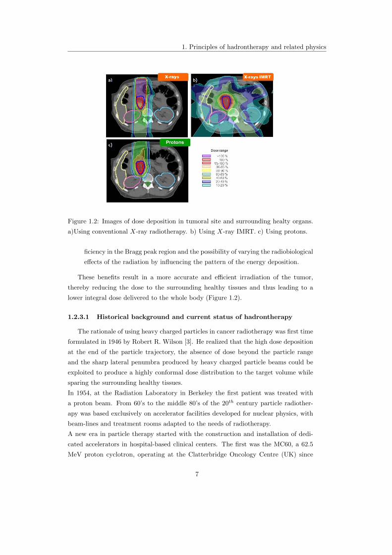
Figure 1.2: Images of dose deposition in tumoral site and surrounding healty organs.
a)Using conventional X-ray radiotherapy. b) Using X-ray IMRT. c) Using protons.
ficiency in the Bragg peak region and the possibility of varying the radiobiological
effects of the radiation by influencing the pattern of the energy deposition.
These benefits result in a more accurate and efficient irradiation of the tumor,
thereby reducing the dose to the surrounding healthy tissues and thus leading to a
lower integral dose delivered to the whole body (Figure 1.2).
1.2.3.1 Historical background and current status of hadrontherapy
The rationale of using heavy charged particles in cancer radiotherapy was first time
formulated in 1946 by Robert R. Wilson [3]. He realized that the high dose deposition
at the end of the particle trajectory, the absence of dose beyond the particle range
and the sharp lateral penumbra produced by heavy charged particle beams could be
exploited to produce a highly conformal dose distribution to the target volume while
sparing the surrounding healthy tissues.
In 1954, at the Radiation Laboratory in Berkeley the first patient was treated with
a proton beam. From 60’s to the middle 80’s of the 20th century particle radiother-
apy was based exclusively on accelerator facilities developed for nuclear physics, with
beam-lines and treatment rooms adapted to the needs of radiotherapy.
A new era in particle therapy started with the construction and installation of dedi-
cated accelerators in hospital-based clinical centers. The first was the MC60, a 62.5
MeV proton cyclotron, operating at the Clatterbridge Oncology Centre (UK) since
7
1. Principles of hadrontherapy and related physics
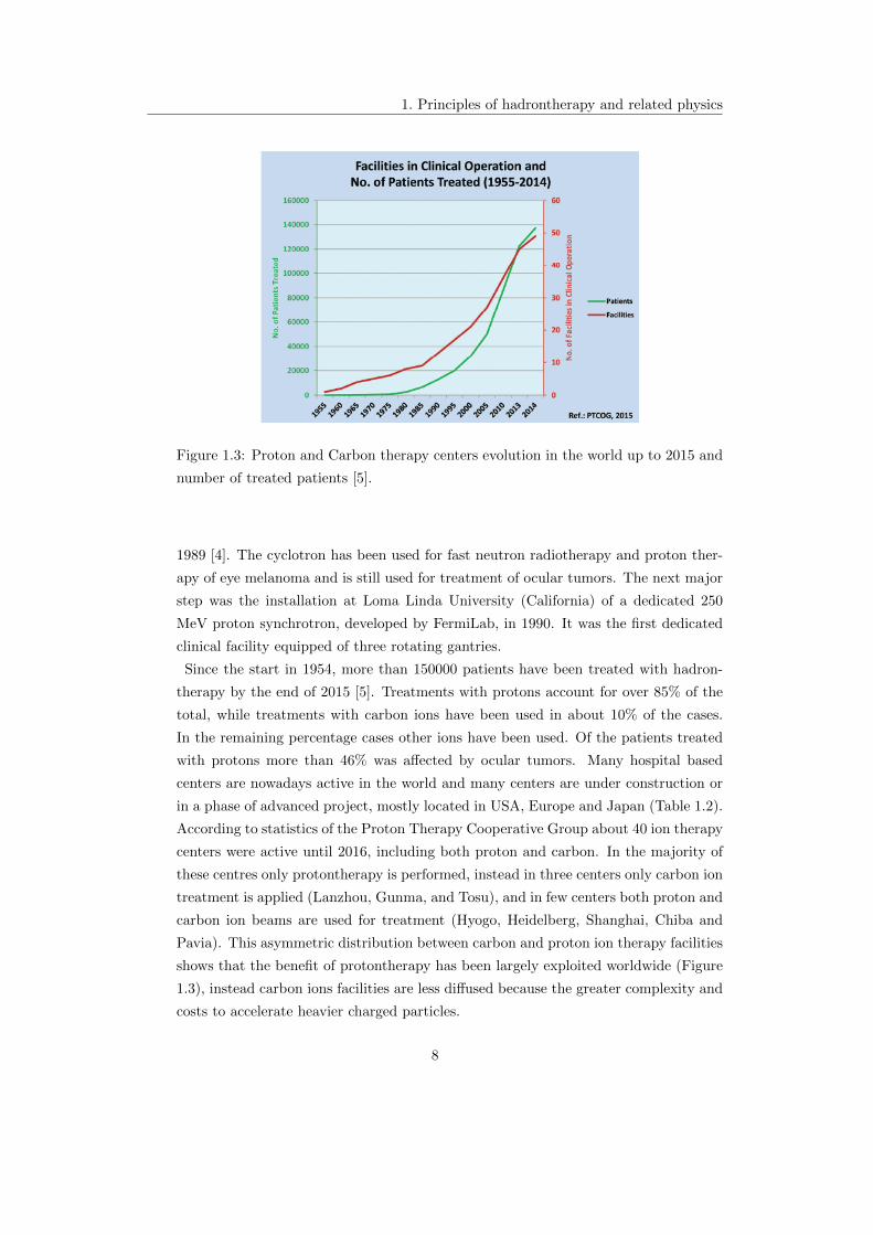
Figure 1.3: Proton and Carbon therapy centers evolution in the world up to 2015 and
number of treated patients [5].
1989 [4]. The cyclotron has been used for fast neutron radiotherapy and proton ther-
apy of eye melanoma and is still used for treatment of ocular tumors. The next major
step was the installation at Loma Linda University (California) of a dedicated 250
MeV proton synchrotron, developed by FermiLab, in 1990. It was the first dedicated
clinical facility equipped of three rotating gantries.
Since the start in 1954, more than 150000 patients have been treated with hadron-
therapy by the end of 2015 [5]. Treatments with protons account for over 85% of the
total, while treatments with carbon ions have been used in about 10% of the cases.
In the remaining percentage cases other ions have been used. Of the patients treated
with protons more than 46% was affected by ocular tumors. Many hospital based
centers are nowadays active in the world and many centers are under construction or
in a phase of advanced project, mostly located in USA, Europe and Japan (Table 1.2).
According to statistics of the Proton Therapy Cooperative Group about 40 ion therapy
centers were active until 2016, including both proton and carbon. In the majority of
these centres only protontherapy is performed, instead in three centers only carbon ion
treatment is applied (Lanzhou, Gunma, and Tosu), and in few centers both proton and
carbon ion beams are used for treatment (Hyogo, Heidelberg, Shanghai, Chiba and
Pavia). This asymmetric distribution between carbon and proton ion therapy facilities
shows that the benefit of protontherapy has been largely exploited worldwide (Figure
1.3), instead carbon ions facilities are less diffused because the greater complexity and
costs to accelerate heavier charged particles.
8

1. Principles of hadrontherapy and related physics
9

1. Principles of hadrontherapy and related physics
Table 1.2: List of all hadrontherapy facilities in the world (in and out of operation)
[4].
10

1. Principles of hadrontherapy and related physics
1.3 Physics of charged hadrons
The different way of releasing energy in matter for different kind of particles is
strictly dependent on the particular interaction that occurs between the interacting
particle and particles composing the traversed tissue.
Charged particles interact with matter primarly throught Coulomb forces between
their positive charge and the negative charge of the orbital electrons of the atoms in the
absorbing material. But, if proton passes close to the atomic nucleus, it experiences
a repulsive elastic Coulomb interaction which, owing to the large mass of the nucleus,
deflects the proton from its original straight-line trajectory. Also inelastic nuclear
reactions between protons and the atomic nucleus may occur. They are less frequent
but are much more interesting because nuclear reaction may be induced. Finally,
radiative energy losses in the form of proton Bremsstrahlung is theoretically possible,
but at therapeutic proton beam energies this effect is negligible.
1.3.1 Electromagnetic interactions
Upon entering any absorbing medium, the hadron immediately interacts with elec-
trons: the electron feels an impulse from the attractive Coulomb force when proton
or other particles passes in its vicinity. In the interaction a fraction of the incoming
particle energy is transferred to the electron and, as a result of the encounter, the
velocity v of the hadron decreases.
Depending on the proximity of the encounter and on the particle energy two situations
may occur:
exitation process: if the impulse may be sufficient only to raise the electron
from one shell to another one of higher energy;
ionization process: if the projectile and the target interact at very close distance
and the primary particle has sufficient energy to remove completely the electron
from the atom.
The maximum energy that can be transferred from a charged particle of mass m
with kinetic energy E to an electron of mass me in a single collision is 4Eme/m, that
correspond to about 1/500 of the incident particle energy per nucleon [7]. This is
only a small fraction of the total initial particle energy, so the primary particle loses
its energy in many interactions as it passes in the material. At any given time, the
particle is interacting with many electrons, so it continuously decreses its velocity and
loses its energy until it is stopped. This energy loss is called stopping power and can
be estimated by the Bethe-Bloch formula [7]
11

1. Principles of hadrontherapy and related physics
−dEdx
= 4πNAZρ
Ar2emec
2 z2
β2
(ln
2mec2β2γ2
I− β2 − δ(γ)
2
)(1.1)
where
for simplicity4πNAr
2emec
2
A = C = 0.307 MeV cm2
g ;
v and ze refer respectively to the velocity and the charge of the incoming hadron;
Z, A and ρ indicate atomic number, mass number and density of the absorbing
material;
me is the rest electron mass;
I represents the mean exitation energy;
δ(γ) is the density effect correction to the ionization energy loss.
For non relativistic charged particles only the first term in parenthesis is relevant.
The main point is the computation of the quantity I. It has to summarize the average
energy spent in exitation and ionization processes, so it is related to the average binding
energy of the atomic electrons. The Bloch approximation [10] gives:
I(eV ) = 10 · Z (1.2)
The calculation of the mean ionization energy is the main source of uncertainty in
the evaluation of the stopping power and the effective path in matter. The standard
value recommended by the Internal Commission of Radiation Units and Measurements
(ICRU) is Iwater = 75 eV, but values in the range 74.6 < I < 81.8 eV are reported in
the literature, with an average value I = (79.2± 1.6) eV [10].
An example of the energy dependence of dEdx is shown in Figure 1.4, which plots
the Bethe-Bloch formula as a function of βγ for different traversed materials. As we
can see, at low energies dEdx is dominated by the multiplicative factor C and decreases
with increasing velocity until a minimum is reached. Particles at this point are known
as Minimum Ionizing Particles (MIP). As the energy increases beyond this point, dEdxrises again due to the logarithmic term, then this relativistic rise is cancelled, however,
by the density correction factor δ(γ). For energies below the minimum ionizing value,
each particle exhibits a dEdx curve which is proportional to 1/v2; this behaviour can be
explained noting that when the velocity v is low, the charged particle spends a greater
time in the vicinity of any electron, so the impulse felt by the electron, and hence the
energy transfered, is larger.
12

1. Principles of hadrontherapy and related physics
Figure 1.4: The Bethe-Bloch curves. Energy loss represented as a function of βγ for
various materials.
Furthermore, as we can see from the equation 1.1, the released energy results pro-
portional to the atomic number z of the incident ion, but the mass m of the incoming
particle does not enter. In particular, the incoming particle enter only through the
proportionality to the square of its charge. It means that for different charged particles
of the same speed, particles with the highest charge will have the greatest energy loss.
Thus, an alfa particle (z = 2) transfers to atomic electrons 4 times more energy than
proton (z = 1) with the same speed.
These two facts are fundamental in hadrontherapy.
1.3.2 Nuclear interactions
When a charged particle passes close to the nucleus it will be elastically scattered
or deflected by the repulsive force from the positive charge of the nucleus. In this case
Multiple Coulomb Scattering takes places (Figure 1.5 right): energy losses are negligible
but it has to be taken into account the angular deviation θ0 of the particle trajectory
from the initial direction. Therefore the observed angular spread of beam traversing
a slab of matter is mainly due to the random combination of many such deflections.
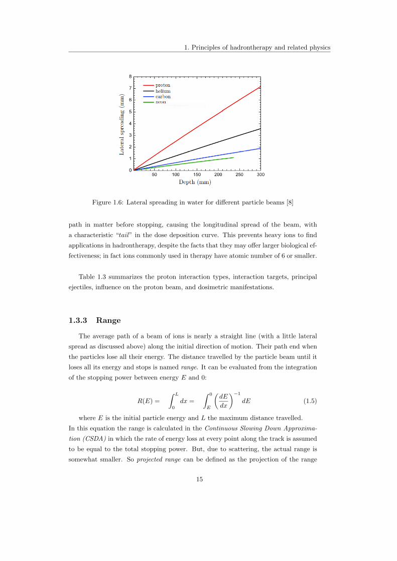
Except in rare cases, the deflection of a hadron by a single atomic nucleus is extremely
small. As can be seen in Figure 1.6, this effect results in a increase of beam transverse
size (cross section) with the depth. From the width of the energy distribution, a
13

1. Principles of hadrontherapy and related physics
measure of the amount of energy straggling (Figure 1.5 left) is achievable:
f(∆E) =1√2πσ
exp
((∆E −∆E)2
2σ2E
)(1.3)
Figure 1.5: Energy distribution of initially monoenergetic charged particle beam at
various penetration distances (left). Multiple Coulomb Scattering in a thin slab (right).
In particular, for hadrons, the widening of a pencil beam is small with respect to
the depth reached and results that the divergence is much more pronounced for elec-
trons (due to theirs smaller masses respect to the mass of the target) than for protons
and heavier nuclei. So this process in many cases can be neglected for hadrontherapy
applications. The angular distribution of protons scattered in a slab of matter is ap-
proximated, in the limit of many collision, by a Gaussian function, with a half width
up to 16 degree, but usually few degrees [12]:
f(θ, d) =1√
2πσθexp
(− θ2
2σ2θ
)(1.4)
where d and θ are respectively the traversed distance and the scattering angle.
Protons, or hadrons, may also interact with the atomic nucleus via inelastic nu-
clear interactions in which the nucleus can be irreversibly transformed, e.g. the proton
is absorbed by the nucleus and secondary particles are produced. As a consequence,
there is a small decrease in the absorbed dose due to the removal of the primary par-
ticle. Another effect is due to heavy charged particles that, interacting with nuclei,
may split in lighter particles. These fragments have a smaller size than the initial ion
but they have a velocity close to that of the projectile. In this way they make a longer
14
1. Principles of hadrontherapy and related physics
Figure 1.6: Lateral spreading in water for different particle beams [8]
path in matter before stopping, causing the longitudinal spread of the beam, with
a characteristic “tail” in the dose deposition curve. This prevents heavy ions to find
applications in hadrontherapy, despite the facts that they may offer larger biological ef-
fectiveness; in fact ions commonly used in therapy have atomic number of 6 or smaller.
Table 1.3 summarizes the proton interaction types, interaction targets, principal
ejectiles, influence on the proton beam, and dosimetric manifestations.
1.3.3 Range
The average path of a beam of ions is nearly a straight line (with a little lateral
spread as discussed above) along the initial direction of motion. Their path end when
the particles lose all their energy. The distance travelled by the particle beam until it
loses all its energy and stops is named range. It can be evaluated from the integration
of the stopping power between energy E and 0:
R(E) =
∫ L
0
dx =
∫ 0
E
(dE
dx
)−1
dE (1.5)
where E is the initial particle energy and L the maximum distance travelled.
In this equation the range is calculated in the Continuous Slowing Down Approxima-
tion (CSDA) in which the rate of energy loss at every point along the track is assumed
to be equal to the total stopping power. But, due to scattering, the actual range is
somewhat smaller. So projected range can be defined as the projection of the range
15

1. Principles of hadrontherapy and related physics
Table 1.3: Summary of proton interaction types, interaction targets, principal ejectiles,
influence on the proton beam, and dosimetric manifestations [11].
along the inital directon of motion.
In general the integration of the Bethe-Bloch equation is not a simple task, so a semi-
empirical relationship, the Bragg-Kleeman formula [10] can be used:
R(E) ≈ αEp (1.6)
where α is a material dependent constant and the exponent p takes into account the
dependence of the proton’s energy or velocity. In this way, the hadron’s range in water,
the main constituent of biological matter, results:
Rwater =
(0.12
keV
µmz2
)−1 ∫ (K
Mc2
)0.82dK
Mc2= (425cm)
A
z2
(K
Mc2
)1.82
(1.7)
Table 1.4 shows kinetic energies request for charged particles used in hadrontherapy
to reach a tumor sited at 25 cm in biological tissue.
Ion z A Rest Energy Kinetic energy [MeV]([MeV/u])
Proton 1 1 938 198 (198)
Helium 2 4 3700 780 (195)
Carbon 6 12 11170 4315 (360)
Neon 10 20 18600 9500 (475)
Table 1.4: Kinetic energies of charged ions corresponding to a range of 25 cm in water.
16

1. Principles of hadrontherapy and related physics
The uncertainty in range calculation may depend on several factors, including the
knowledge of the proton beam energy distribution and on properties of all absorbing
materials in the beam path. Another source of uncertainty is due to the fact that the
calculation of range from the previous formula gives an average value that does not
take into account the effect of nuclear collisions along the particle trajectory.
Interaction with nuclei are also responsable of range straggling, defined as the fluctu-
ation in path lenght for individual particles of the same energy, resulting in a sightly
different total range for each particle. The resulting range spreading σR is related to
the energy straggling σ:
σR =
∫ (dE
dx
)−3dσ
dxdE (1.8)
This equation can be solved to determine the evolution of the range straggling variance
as a function of depth x. For light ions the relative range straggling is around 0.1%,
going on with z this value diminishes: in particular for C-ions the range straggling
is 3.5 times smaller than for protons [10]. This fact makes it possible for hadrons
to neglect nuclear interactions in the range calculation. In this approximation the
penetration in matter pratically equals the lenght of the actual path. This fact is of
extremely importance in hadrontherapy, because make it possible the exact calculation
of particles range in tissues.
1.3.4 Linear Energy Transfer
The Bethe-Bloch formula makes possible to compute the incident particle energy
losses per unit of path, in ionization processes. But, medical phisycists are more in-
terested in the calculation of quantities that can be directly correlated to the damages
to the tissues.
If a charge particle of energy E moves in a medium it loses its energy, but only a
fraction of the particle energy is transfered to the tissues, causing ionizazions; instead
another fraction is lost in the form of bremmstrhalung, so escapes the patient, and
does not cause any cellular damages.
To take into account only the first contribute, the Linear Energy Transfered can be
defined as the amount of energy ∆E released in matter per unit of path length ∆x
LET =∆E
∆x(1.9)
or, analogously, as the product of specific ionization (IP/cm) and the average energy
deposited per ion pair (eV/IP). From these two definitions it is clear that LET of a
17

1. Principles of hadrontherapy and related physics
particular type of radiation expresses the energy deposition density, which largely
determines the biological consequences of radiation exposure. It is usually expressed
in units of eVcm or keV
µm .
For a more precise calculation [8] it has to be considered that in these processes,
the projectile of kinetic energy E loses an energy δE = Eel + I, where Eel is the
kinetic energy transferred to the outcoming electron and I the ionization potential of
that electron. Most of the electrons are stopped near their emission point but, some
of them, have sufficient energy to deposit their energy far away. Hence, the energy
absorbed locally by the material is not strictly equal to the stopping power. So, more
precisely, the Linear Energy Transfer should be calculated as follow:
LET =
(dE
dx
)−∑
Eel (1.10)
where∑Eel is the total kinetic energy of ejected electrons, named δ electrons.
But, some δ electrons are also coming from the previous elementary volume and will
deposit their energy in the elementary volume in consideration. This roughly balances
the energy of δ electrons produced in that volume, so in a first approximation we can
identify the Stopping Power and the LET in the elementary volume of thickness dx:dEdx ' LET .
Since water is the principal costituent of all type of biological tissues, it is resonable
to compute LET in water to extimate the particle energy deposition in tissues:
LETwater = 0.12keV
µmz2
(Mc2
K
)0.82
(1.11)
where K is the kinetic energy of particle having rest energy equal to Mc2.
Using the above expression, the LET can be expressed as a function of k = KMc2 ,
the fractional kinetic energy of the incoming particle, because the only relevant pa-
rameter is the square of the velocity. The double-logarithmic graph, in Figure 1.7,
shows that, for fractional kinetic energies smaller than about 0.4 (i.e. for v/c < 0.7)
the LET can be represented by a straight line. This implies that a simple power law
can be used to describe the LET for the kinetic energies used in hadrontherapy. ForKMc2 larger than 1 the particles are relativistic and the velocity does not increase any
longer with energy: the LET is practically constant and equal to 0.21 keVµm . Instead, in
the range 0.4 < k < 1 no simple rule applies. The LET is strictly dependent from type
of particle and its energy, in fact it results proportional to the square of the charge and
inversely proportional to the particle’s kinetic energy, hence to the velocity. For fixed
target, LET is only dependent on the atomic number z of the projectile and from its
velocity. In particular, as can be seen by the dEdx expression, for different particles of
the same velocity, the higher is the particle charge, the higher results the linear energy
18

1. Principles of hadrontherapy and related physics
transfered to the tissues.
Figure 1.7: LET as a function of k = KMc2 .
In general, considering LET, particles can be divided into:
high LET radiations or densely ionizing particles: such as alpha particles,
carbon ions and light ions in general. These types of radiation realease in matter a
great amount of energy for unit of path, sufficient to produce very close ionizazion
processes, causing damages to tissues. The LET stays is in the range 1−100keVµm .
low LET radiations or sparsely ionizing particles, which include electrons
and electromagnetic radiation, but even protons. The ionization events deriving
from the interactions of these particles with matter are much more distant than
the previous, so the damages caused to the cancerous cells results less effectives.
The LET is in the range 0.1− 1keVµm .
1.3.5 Bragg curve
The rationale for the use of proton, or in general hadron, beams in radiation ther-
apy stands on the physical characteristics of energy loss when they traverse matter,
allowing a better dose distribution to the target compared to conventional radiother-
apy tecniques.
In fact hadrons exhibit a relative low ionization density in the first part of their path
in the material (tissue), resulting in a small dose deposition in the first centimetres of
penetration depth. Instead dose deposition slowly increases, reaching a narrow maxi-
mum at the end of the particle range where the ionization density is very high. This
19

1. Principles of hadrontherapy and related physics
trend of the absorbed dose as a function of the reached depth is named Bragg Curve,
and the region around the maximum dose deposition is the Bragg Peak.
Figure 1.8: Evolution of the relative dose with respect the penetration depth in water
for different particles.
The blue curve on Figure 1.8 shows the dose deposition of a 107 MeV proton beam
with respect to the penetration depth of the protons in water. The red curve corre-
sponds to the dose deposition of a carbon ion of 200 MeV/u. For both projectiles, it is
clearly seen that the maximum deposition is located at the end of the path in a quite
sharp peak.
The general structure of the Bragg curves can be understood very easily: at high en-
ergy the energy loss is small and the particles travel along the trajectory producing
a low and nearly constant ionization density (plateau region); but, as the particles
energy slow down, LET increases rapidly (as K−0.82, according to the equation 1.11),
and the narrow peak appears. Physically, the Bragg peak does not diverge because,
before stopping, the hadron spends its remain energy to capture atomic electrons, in
this way the particle becomes neutral and loses its capacity to ionize.
It has to be noted that the dose deposition before the Bragg peak is small (from
10% to 20% of the maximum [8]) both for protons and carbon ions. But after the
peak there is no dose deposition for protons and a weak dose deposition for carbon.
This tail of dose deposition is due to the fragmentation of the projectile. In fact, as the
20

1. Principles of hadrontherapy and related physics
mass of the projectile increases, the interaction with the target can cause the break
of the ion, originating charged ions of minor masses, able to produce other ionization
events beyond the Bragg peak region.
The location of the Bragg peak only depends on the particle incident energy, instead
its widening is due to the energy spread.
Because the peak deriving from a monoenergetic hadron’s beam is extremely narrow,
it is not sufficient to cover the entire extention of the tumor. So, to paint all the
volume of a tumor, different beam energies are used during the treatment, giving rise
to a plateau region called Spread Out Bragg Peak, SOBP (Figure 1.9). In this way, by
the properly modulation of the initial beam energy it is possible to irradiate accurately
the tumor with a weak dose deposition on the tissues located before the Bragg peak
and with a very small dose released beyond the Bragg peak. This fact is the main
advantage of the hadrontherapy treatments, because it allows to release a great amount
of dose exactly in the tumoral site, and at the same time, giving very low dose to the
surrounding organs resulting, in this way, a less invasive tecnique than conventional
radiotherapy.
Figure 1.9: Superposition of proton beam of different energies creating Spread out
Bragg Peak.
21

1. Principles of hadrontherapy and related physics
1.4 Radiobiological properties of hadrons
All biological organisms consist of cells as the basic units. Every cell has a nucleus
containing DNA molecules that carry all the genetic informations used in the develop-
ment and functions of all living organisms. Many experiments have confirmed that the
DNA represents the main target for radiation damage. Also the other molecules may
be damaged from the radiation exposure, but they can be simply replaced by others of
the same species. DNA is composed by two long polymeric chains called double strand
and it is organized into structures called chromosomes, which constitute the targets
for irradiation. If these structures are seriously damaged from radiations, the damage
cannot be repaired and affects lethally the function and the reproductivity of the cell
giving rise to cell death or to genetic mutations.
1.4.1 Radiation damage to DNA
Irradiation of any biological system generates in sequence, a succession of processes
differing enormously on a time scale basis. We can distinguish three main phases:
Physical or direct phase: as an immediate consequence of radiation energy depo-
sition in a biological system physical effects occur in the time scale of up to 10−13
s. Atoms of target are ionized or exited by direct irradiation with a consequent
production of electrons, as described in the previous section.
Chemical or indirect phase: the secondary radiations (electrons), make interac-
tions with water molecules in the target and can produce free radicals, OH−
ions. They, in turn, can interact with other cellular components and several
chemical reactions take place. In the most common forms of radiation therapy,
the most of the radiation damages is due to free radicals. All these processes
occur on a time scale of 10−3 s.
Biological phase: it begins with enzymatic reactions that take place on the resid-
ual chemical damage, after few hours from the radiation exposure. The majority
of lesions are, at this time, succesfully repaired, but some of them lead to cell
death producing biological effects, such as cancer, that may be observed within
the time scale of up to several tens of years.
Every cell is equipped with a mechanism for repairing DNA damages, when they
occur. But this mechanism is valid only if the ionization events are largely spaced and
if they cause the breaking of only one of the DNA helix. In this case the funtionality
of the cells is restored with minor or no consequencies. On the other hand, if the
radiation energy is sufficiently high, ionizations occur much more closely in space and
22

1. Principles of hadrontherapy and related physics
may cause double strand breaking. In this situation the cell dies or cannot reproduce.
Experimental evidence [1] showed that most of the cells are killed by high LET radia-
tion, when the ionization density is around 10-100 keVµm . The typical distance between
the two DNA strands is about 2 nm so, to kill cancerous cells, ionization events distant
about 2 nm have to be produced. For exemple, the LET in water in the last 40 mm
track of 400 MeV/u carbon ions of is LETwater = 20 keVµm . Since the energy to produce
a ion pair in water is about 40 eV the average distance d between two ionizations
results d ' 40LET eV=2 nm (Figure 1.10).
Figure 1.10: Structure of a proton and a carbon track, in nanometric resolution,
compared with a schematic rapresentation of DNA.
Table 1.5: LET values at various residual range for different particles.
As we can see from the Table 1.5 protons of E = 200 MeV show low LET in water,
so they are classified as sparsely ionizing, but just before stopping LET reaches a high
23

1. Principles of hadrontherapy and related physics
value that corresponds to a distance d of few nm between ionization events.
1.4.2 Relative Biological Effectiveness
As mentioned above, one advantage of hadrontherapy lies in the biological effects
induced by these charged particles. The differences in the effects produced by radiation
of various type for the same physical dose are accounted by introducing the Relative
Biological Effectiveness, RBE.
The RBE of a given radiation is defined as the ratio between the absorbed dose of a
reference radiation, e.g. X-ray, and that of the test radiation, required to produce the
same biological effect, i.e. to kill the same amount of cells. In general, tipical radiation
reference are 250 MeV X-ray or 1.2 MeV γ’s emitted by 60Co.
RBE =DX−ray
Dtest(1.12)
Despite the simplicity of the definition, RBE is a complex quantity depending not
only on the absorbed dose, but also on the type of particle, type of target tissue, dose
fration, delivery methods, etc...
Figure 1.11: RBE = f(LET ) The LET range for protons is indicated by the blue
area. The red area corresponds to the 12C LET range [8].
RBE seems to be strongly related to LET, as shown in Figure 1.11. RBE for pro-
tons, whose LET is in the range 0.5 to 3 MeV/mm is close to 1. On the other hand
RBE of carbon, whose LET ranges between 20 and 250 MeV/mm, varies signficantly
24

1. Principles of hadrontherapy and related physics
between 1.3 and 3 reaching a maximum. It would mean that densely ionizing radi-
ations have higher biological effect than sparsely ones. However, if LET values are
too high, ionization events becomes extremely close causing an overproduction of local
damage in a small volume and a consequent decreasing of RBE (overkill-effect).
The RBE is operatively measured by the fraction of cell survival as schematically pre-
sented in Figure 1.12. The shape of these curves is a very important factor to measure
quantitatively the killing effect of radiation of different qualities on the populations of
irradiated cells. It is reported in a semi-logarithmic scale the fraction of cells surviving
the irradiation as a function of the absorbed dose, both for the reference radiation and
for the radiation in exam.
Figure 1.12: Survival curves and determination of RBE for a 10% of cancerous cells
survival.
The compromise between the necessity to destroy the tumoral cells and those to
maintain the dose to the surrounding healthy tissues within the limits, can be obtained
from the analysis of the so called dose-effects curves (Figure 1.13). They represents:
for cancerous tissues, the probability of obtaining the desired effect as function
of the dose delivered;
for healthy tissues, the probability of causing damages, always as function of the
dose absorbed by the same tissue.
As can be seen in Figure 1.13 to obtain the probability of local control of the tumor
close to 1, an amount of absorbed dose is necessary, also corresponding to a very high
probability of causing complications in healty tissues. The compromise is represented
by the therapeutic ratio, defined as the ratio D1/D2 between the dose corresponding
to 50% probability of producing complication and the amount of dose necessary to
obtain the same percentage of local control [6].
25

1. Principles of hadrontherapy and related physics
Figure 1.13: The dose-effects curve. It represents the probability of complications or
tumor control as a function of the absorbed dose.
1.4.3 Oxigen Enhancement Ratio
Another biological effect to take into account is the so called “Oxygen effect”. The
cells with low oxygenation rate (hypoxic cells) are more resistant to radiations than
cells with a normal content of oxygen (aerobic cells). As a consequence, more dose is
needed to destroy hypoxic cells. Unfortunately, cancerous tissues are generally very
poorly vascularized and, therefore, are very low in oxygen. For this reason the effect
of radiation on this kind of tissues decrease. This effect is parametrised by the Oxygen
Enhancement Ratio (OER) which is defined as follows:
OER =Dhypoxic
Daerobic(1.13)
whereDhypoxic is the dose needed to kill a fixed amount of hypoxic cells andDaerobic
is the dose needed to kill the same amount of aerobic cells. The OER value clearly
depends on the LET value: in a first approximation, OER is a decreasing function of
LET. For X-rays the OER value stays around 3. Protons have OER value similar to
ones of X-rays. For high LET values like carbon at low energies (close to the Bragg
peak), the OER value decreases down to 2. RBE and OER trends are summarized on
Figure 1.14.
For ions heavier than Neon the OER value is close to one: the Oxygen Effect has
almost disappeared. This means that high LET radiations have the same effect on the
tumor tissue regardless the amount of oxygen and, therefore, are much better indicated
26

1. Principles of hadrontherapy and related physics
Figure 1.14: OER and RBE as a function of LET.
in radiation therapy than electrons or photons.
27

Chapter 2
Equipment for hadrontherapy
facilities
A typical hadron therapy facility comprises several main components (Figure 2.1)
that interact each other to deliver the proper dose to the patients:
an accelerator with an energy selection system to produce beams of suitable
energies;
a beam transport system to steer the beam to the treatment delivery system;
a treatment delivery system, for conformation and delivery the dose to the target
tumor. It comprises in turn several subsystems such as the gantry, the treatment
coach, and the patient-positioning and immobilization devices.
a a dose delivery monitor to control that the prescribed dose is properly and
accurately delivered to the patient;
a control system that report on the status of all components and eventually raise
warning or alarms;
a treatment planning system, a complex piece of software that plan how and
where the beam shall be delivered, according to clinical prescription.
2.1 Accelerator systems for hadrontherapy
Until the 90′s protontherapy has been developed slowly because it was performed
in nuclear physics laboratories that were equipped with a particle accelerator. When
28

2. Equipment for hadrontherapy facilities
Figure 2.1: A schematic view of a hadrontherapy facility.
the efficacy and success of protontherapy became more established, dedicated facilities
started to emerge.
The energies require for the treatment with hadrons of deep seated tumors range, typi-
cally, between 60 and 250 MeV for protons until 120-450 MeV/u for carbon’s ions. The
therapeutic hadron beams can be currently produced by three classes of accelerators:
cyclotrons, synchrotrons and linear accelerators.
Nowadays the cyclotron and the synchrotron are the two types of accelerators prefer-
ably used in the dedicated hadrontherapy centres. Nevertheless, this field of reaserch
is in countinuos development, in fact in the last years new technologies combining
different types of accelerating machines have been proposed with the aim to produce
particle beams more suitable for medical applications (Table 2.1). These options are
at very different stages of design maturity, but all offer promising design features to
offset the shortcomings of current accelerators, including fast scanning capabilities,
reduced size, complexity and power consumption, increased dose rate capability, and
ultimately a lower cost and a shorter treatment time.
29

2. Equipment for hadrontherapy facilities
Table 2.1: A comparison of the main features of the present and future accelerators
for charge particle therapy [10].
2.1.1 Cyclotron
From the beginning of protontherapy the cyclotron has been used for applications
in the medical field such as radionuclides production. The main reasons of this choice
lie in its relatively simple design and operation mode, in fact it works at fixed magnetic
field and constant energy.
The typical stucture of a compact cyclotron is the following:
An ion source is located in the center of the cyclotron;
A radio frequency (RF) system provides a strong electric field which acceler-
ates the charged particles between two D-shaped hollow electrodes called dees,
installed between the poles of large electromagnets;
An extraction system that guides the particles that have reached their maximum
energy out of the cyclotron, into a beam transport system.
In a system of this kind every particle is subject to the effects of two different forces:
the Lorentz force, which tends to curve the particle trajectory, and the centrifugal force
which on the contrary tends to restore the linear motion and whose magnitude will be
equal to that of the Lorentz force:
qvB = mv2
r(2.1)
where q, m and v are respectively charge, mass and velocity of the accelerated
particle, r is the radius of the particle’s trajectory, and B is the applied magnetic
30
2. Equipment for hadrontherapy facilities
field.
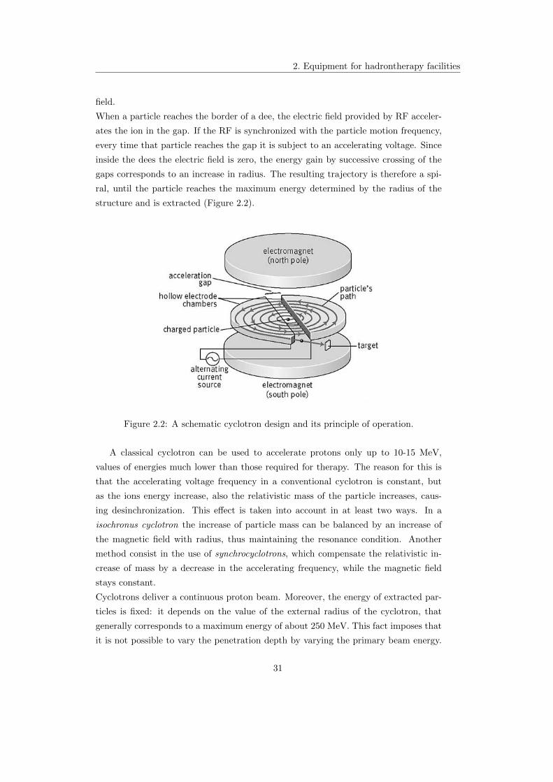
When a particle reaches the border of a dee, the electric field provided by RF acceler-
ates the ion in the gap. If the RF is synchronized with the particle motion frequency,
every time that particle reaches the gap it is subject to an accelerating voltage. Since
inside the dees the electric field is zero, the energy gain by successive crossing of the
gaps corresponds to an increase in radius. The resulting trajectory is therefore a spi-
ral, until the particle reaches the maximum energy determined by the radius of the
structure and is extracted (Figure 2.2).
Figure 2.2: A schematic cyclotron design and its principle of operation.
A classical cyclotron can be used to accelerate protons only up to 10-15 MeV,
values of energies much lower than those required for therapy. The reason for this is
that the accelerating voltage frequency in a conventional cyclotron is constant, but
as the ions energy increase, also the relativistic mass of the particle increases, caus-
ing desinchronization. This effect is taken into account in at least two ways. In a
isochronus cyclotron the increase of particle mass can be balanced by an increase of
the magnetic field with radius, thus maintaining the resonance condition. Another
method consist in the use of synchrocyclotrons, which compensate the relativistic in-
crease of mass by a decrease in the accelerating frequency, while the magnetic field
stays constant.
Cyclotrons deliver a continuous proton beam. Moreover, the energy of extracted par-
ticles is fixed: it depends on the value of the external radius of the cyclotron, that
generally corresponds to a maximum energy of about 250 MeV. This fact imposes that
it is not possible to vary the penetration depth by varying the primary beam energy.
31

2. Equipment for hadrontherapy facilities
For this reason each cyclotron is coupled with a variable thickness energy degrader
and energy selector, which aims to reduce the 250 MeV monoenergetic proton beam
to an arbitrary energy down to about 60 MeV. However, the decreasing of proton en-
ergy leads to the reduction of the proton current up to two orders of magnitude, which
might be inconvenient for some application, e.g. eye treatment. Furthermore absorbers
and magnetic filters produce high neutron fluxes and significant component activation,
causing induced radioactivity that has to be correctly controlled and disposed off.
2.1.2 Synchrotron
The principle of operation of a synchrotron consists in keeping particles in motion
around a circular path, with fixed radius r = pBq = const. To accomplish this task
is necessary to apply a magnetic field variable in time. But to achieve acceleration
also the frequency of RF must be synchronized with the revolution frequency of the
particles in the changing magnetic field.
A synchrotron itself consists in:
a iniector, typically a small linear accelerator that provides particles of few MeV
then injected into a ring. To obtain the correct acceleration the injection must
be done at the correct phase with respect to the RF of the ring.
a circular sequence of bending magnets and focusing elements.
an extraction system, to drive the particles of the desired energy out of the
accelerator.
Although proton synchrotrons is largely used in the most of the high energy physics
experiments, the features of the particle beam produced by this machines permit also
its use in biomedical applications.
The major advantage of synchrotrons is that they can reach energies up to 1000 times
higher than those reached by a typical cyclotron. So, not only protons, but also heav-
ier ions can be accelerated. Furthermore, with a synchrotron it is possible to extract
beams of any energy: in this way the properly energy modulation can be achieved
without any absorbing material, reducing the associated beam losses and high radia-
tion levels.
After the particles have been extracted, both the magnetic field and the electric field
frequency have to be restored to their initial values to ensure that a new group of
particles can be accelerated. Tipically the beam acceleration cycle takes from ∼ 200
ms to ∼ 1 s and beam extraction occurs over a similar period. The consequence of this
fact is that the particle beam in output is pulsed, with a repetion rate ranging between
0.5 Hz and 2 Hz. In this way the beam is not always present during the hadrontherapy
32

2. Equipment for hadrontherapy facilities
treatment and can be absent for at least one second. This is an incovenient because,
for exemple to treat more precisely organs that move under the patient’s breathing
cycle, usually the beam has to be synchronized with the expiration phase, that in this
case cannot be directly correlated to the synchrotron cycle.
As we have be seen for the cyclotron, also the particles accelerated by synchrotrons
are subject to radiative energy losses, causing induced radioactivity.
2.1.3 Linear Accelerators
Linear accelerators are widely used in radiation therapy to accelerate electrons,
tipically between 6-25 MeV. A general LINAC is composed by a modular sequence
of accelerating structures, consisting in waveguides or resonant cavities excited by a
radiofrequency electromagnetic field.
Accelerated electrons quickly reach relativistic velocities which implies identical repet-
itive acceleration cavities working at the same phase. On the other hand, protons
event at the maximum therapeutic kinetic energy of 250 MeV are still non relativistic,
so to mantain synchronism with the alternating electric field applied, the accelerating
modules must have an increasing lenght. The lenght of the n module is given by [13]:
Ln =1
2f
√2qV n
m(2.2)
where V is the applied voltage, q the particle charge and m its mass, f is the frequency.
A linear accelerator produces a pulsed beam, with short pulses of ∼ µs at high repeti-
tion rate (100-200 Hz). This time structure may have important positive consequences
for the beam delivery system. But, if all the accelerating modules are active, the out-
put energy from linear accelerator is fixed. Nevertheless energy modulation can be
achieved by switching off the output RF power of a number of modules and by ad-
justing the power of the last active cavities. In this way the final energy can be varied
for each pulse, giving the possibility of active three-dimensional scanning of the tumor.
2.1.3.1 Advantages and disadvantages of proton-LINAC
Linear accelerators are typically characterized by the production of high-energy
and high-intensity charged particle beams of high beam quality, which means small
beam emittance and small energy spread. The main features of proton linac can be
summarized as follow:
single pulse energy modulation and high repetition rate, as pointed out above.
33
2. Equipment for hadrontherapy facilities
modular structure that makes possible the progressive installation and test of
each module and also the immediate exploitation of the beam, even with partial
deployment of the modules.
no power loss from synchrotron radiation, because the beam travels along a
linear trajectory simplifying significantly the radioprotection aspects (and then
reducing risks and costs). Moreover, since the beam traverses the accelerator
only one time, repetitive errors causing destructive beam resonance are avoided.
the injection and extraction systems are simpler than in circular accelerators,
where additional components have to be added.
Probably, the main disadvantage presented by a LINAC is that it is a machine
strictly dependent from the nature of the accelerated particle beams. In fact, to
accelarate particles with different masses, cavities with different lenght are request,
accordingly to the above expression. This would mean that each hadron LINAC can
be used only to accelerate one type of ions.
2.2 Dose delivery systems
The dose delivery system represents a key issue in the full treatment process since
allows the conformation of the beam coming out from the accelerator into a 3D dose
distribution, according to a predetermined treatment plan.
There are two general methods to shape the beam to the tumor: the passive scattering
system, until now the most widely used in almost all radiotherapy centers, and the
more recent active scanning systems, which are expected to become the standard in
the near future.
2.2.1 Passive beam delivery system
In passive beam delivery systems the right dose distribution is obtained by the
interposition of mechanical devices along the beam path, in order to shape it to the
tumor, using the particle-matter interactions.
To adapt the lateral beam profile to the lateral dimensions of the lesion, scatterers
are used (Figure 2.3). They spread the originally Gaussian beam profile into a wide
uniform profile that is adapted to the dimensions of the tumor using patient-specific
collimators. Rotating wheels of various thickness are applied as energy modulators.
Their task is to gradually degrade the initially beam energy to cover the entire ex-
tention in depth of the tumor. Finally, longitudinal compensation has to be applied
to account for tissue inhomogeneities and the curvature of the target, especially when
34

2. Equipment for hadrontherapy facilities
Figure 2.3: Principle of passive beam application (upper part: schematic setup; lower
part: variation of lateral and longitudinal beam profile along setup).
critical structures are close to the distal edge of the treated volume. To achieve this
compensator devices, drilled for each field and each patient, are used. But, while the
distal edge of the dose deposition can be adapted very precisely to the target volume,
the fixed shape of the SOBP cause the translation of the distal shaped dose distribu-
tion for the entire depth of the tumor, resulting in unwanted irradiation of surrounding
healthy tissues. Also extra dose is somministred to the patient due to the neutrons
produced by the beam scattering with the various components (Figure 2.3). These
nuclear interactions occurring in the scattering system cause fluence losses that lead
to a low efficiency of the passive delivery systems, between 3% and 30%.
2.2.2 Active beam delivery system
The use of degraders to shift energy range can be avoided if the accelerator itself
allows the variation of the output beam energy, as in synchrotrons and linear acceler-
ators.
The active or dynamic beam delivery is an innovative system that exploits the ballistic
properties of charged particles much better then passive methods.
This tecnique consists in both transverse and longitudinal scan of the tumor. This
can be achieved by means of “pencil” beams, delivered in time sequence, coming di-
rectly from the accelerator, without passing any absorbing materials. By the properly
modulation of the exit beam energy, the position of the Bragg peak can be varied:
in this way the tumor can virtually be divided in many “slices”, each one receiving
the correct amount of dose. Scanning in horizontal and vertical directions is obtained
deflecting the beam by means of two bending magnets as can be seen in Figure 2.4.
35

2. Equipment for hadrontherapy facilities
Basically, two types of active scanning exist:
the spot scanning is a discrete scanning method. As soon as each pencil beam
releases its amount of dose, the beam is switched off for about 2 ms, during which
the magnets are moved in order to direct protons in the next voxel. The beam
spot is moved in large steps, of the order of the FWHM1 of the spot ∼ 8 − 10
mm.
in the raster scanning a pencil beam of 4-10 mm width (FWHM) is moved in
the transverse plane almost continuously. After painting a section of the tumour,
the energy of the beam extracted from the synchrotron is reduced to paint a less
deep layer. In practice to obtain a variable speed the beam is moved in steps
much smaller than the FWHM of the spot. In such approach the beam is always
on.
Figure 2.4: Principle of active scanning dose delivery system: the magnets move the
beam in the transverse plane; the energy modulation permits the longitudinal scan of
the tumor.
2.3 Dose delivery monitor
The dosimetric control is a fundamental task in radiotherapy that has to be per-
formed by means of appropriate monitoring systems in order to be confident on the
dose delivered.
To successfully exploit the high level of precision potentially achievable with protons,
and at the same time minimize the higher potential risk of overshooting, all beam
properties regarding the treatment must be keep under control during all the time of
1Full With at Half Maximum of the Gaussian energy distribution of the beam spot.
36

2. Equipment for hadrontherapy facilities
the exposure. To achieve this purpose an accurate beam monitoring system has to be
installed along the beam path, just before the patient.
The main purpose of the monitoring system is to verify in real time the exact corre-
spondence between the prescribed dose and the dose delivered during the treatment
with an uncertainty which must be contained within a few percent. To achieve this
objective, precise measurements of beam position, profile and intensity have to be ob-
tained in real time, to ensure that the irradiation takes place according to the methods
estabilished by the treatment plans. Also, a system of this type would be able to stop
the beam once the prescribed dose has been reached or if at least one of the beam
parameters is out of the acceptance range.
The accurate measurement and monitor of the radiation spatial distribution, along the
beam trajectory, assume fundamental importance also because it shows how the beam
is modified by the interactions that occur before reaching the patient. For exemple
the nuclear interactions with the components of the passive dose delivery system can
cause deflections or induce divergencies of the beam.
In principle, if the beam is properly tuned and the beam delivery is functioning cor-
rectly, one calibrated detector is sufficient for the measure of the delivered dose. How-
ever, depending on the complexity of the beam delivery system, several detectors are
needed to obtain the required level of accuracy and safety. Generally, several indepen-
dent (with some sort of hierarchy) devices are required to ensure redundancy.
For dosimetry in hadrontherapy, also reproducibility in beam delivery has to be high.
In addition to the spatial resolution, it is also desirable have detector, with well know
(and simple) response respect to beam energy, LET and possibly linear with dose in the
region of interest. Depending on the task, dosimetry detector systems have different
specifications. For instance, the spatial resolution required when for quality assurance
measurements can be different for beam scanning compared to passive scattering. Also,
the time structure of the beam delivery and thus the local energy deposition might
differ in the detector geometry potentially affecting measurement accuracy. Dose-rate
linearity is an important requirement in scanned beams. Furthermore, in scanned
beam delivery, depending on the scanning pattern, it may take longer to accumulate
the dose over time [10].
In the next paragraph we will describe more in detail the principles of operation of
detectors mostly in use for radiotherpy applications.
37

2. Equipment for hadrontherapy facilities
2.3.1 Radiation detector for medical applications
Several types of radiation detectors are used in clinical applications. They, accord-
ing to their function, can be classified in:
detectors for absolute calibration measurements. They must be based on a pri-
mary standard which provides the reference absorbed dose unit by an absolute
measurements, without any previous calibration.
radiation detectors that can be used to measure the dose, after being calibrated
for a particular type of radiation;
specialized detectors that measure the properties of certain particles, such as
scattering angle of the incident particle.
2.3.1.1 Ionization chamber
Several of the most widely used radiation detectors are based on the effects pro-
duced when a charged particle passes through a gaseous medium.
In many treatment centers with heavy particles beams, the choice falls on ionization
chambers, which are often used as key devices to measure the dose because of theirs
accuracy, reliability and ease of operation. These instruments are based on the direct
collection of the ionization electrons and ions produced in a gas by passing radiation.
The total number of ion pair created along the track constitues the real quantity of in-
terest, since it constitues the basis of the electric signal developed by the ion chamber.
Also, the mean number of pairs created results proportional to the energy deposited
by radiation in the counter, which in turns is proportional to the dose absorbed by the
detector. More precisely the exact calculation of the absorbed dose can be achieved
by the Bragg-Gray formula:
D =QwiρV
(2.3)
where Q is the charge produced by the ionization events, wi is the energy requests to
produce a ion-electron pair in the gas, ρ is the density of the gas and V is the chamber
active volume. The amount of ionization produced per unit of deposited energy is a
function of the type of radiation. However, for proton and light-ion beams at clinically
energies there is only a weak dependence of the wi value on particle type: values of
34.3 eV and 33.7 eV are measured for protons and for heavier ions in air [6]. Values
of wi for other gases are recommended by ICRU [16].
Since, the exact calculation of the dose absorbed in biological tissues assumes ex-
treme importance, both for therapy and radiation protection, “tissue-equivalent” ion
chambers are widely used. These type of monitor sistems are constructed using light
38

2. Equipment for hadrontherapy facilities
material with a composition similar to that of biological tissues.
The most common type of ionization chamber configuration used in beam mon-
itoring system is transmission ion chamber. The basic configuration consists of two
parallel conductive planes, with the role of electrodes, separated by a gap of few mil-
limetres (Figure 2.5). The gap volume is filled by a suitable gas. Air is the most
common filling gas and is one in which ionization readily occurs. Denser gases such
as Argon are sometimes chosen in other applications to increase the ionization density
within a given volume. The gas pressure is often one nominal atmosphere, although
higher pressures are sometimes used to increase the sensitivity.
A negative voltage is applied between the two electrodes to create an electric field
inside the gap. Usually the high voltage supply is connected only to one electrode,
the chatode, while the anode is linked to the front-end electronics, allowing the mea-
sure of the electron charge. In fact, when the incident radiation ionizes the filling gas
atoms, under the influence of the electric field, the positive ions will be accelerated
towards the chatode and the electrons toward the anode, where they are collected. The
charge flux generates an ionization current that is measured by an electrometer circuit.
Figure 2.5: View of a typical trasmission ionization chamber.
Also, thimble ionizazion chambers are used. The principle of operation is the same
of the trasmission ones but a chamber of this type is composed by a cylindric con-
tainer with conductive walls, filled by gas. Along its axis is suspended a conducting
wire to which a positive voltage relative to the walls is applied. In this way a radial
electric field is estabilished. Smaller the chamber worst is the sensitivity, but better
39

2. Equipment for hadrontherapy facilities
the spatial resolution. These sensors are used mainly as a pratical secondary reference
instruments after calibration again primary standard.
It is worth mentioning the typical charge collection timing in a ionization chamber.
If an electric field is applied in the gas, the electrostatic forces will tend to move the
charges away from their point of origin. The charges motion consists of a superposition
of a random thermal velocity and a net drift velocity u in a given direction. It is useful
to define the mobility µ of a charge as
µ =u
E(2.4)
where u is the drift velocity and E the electric field strength. The electrons mobility
is much greater than that of positive ions, because their smaller mass allows a greater
acceleration between encounters with neutral gas molecules. The value of electron
mobility is tipically 1000 times greater than that of ions: in Air, results approximately
µe ∼ 1 cm2
µs·kV while the heavier ions drift at mobility of about µN ∼ 3 × 10⁻³ cm2
µs·kV .
From these numbers, the typical transit time of electrons and ions in a 2 mm ionization
chamber with a bias voltage of 200 V (or electric field of 1 kVcm ) is respectively: 200 ns
and 60 µs [17].
Collisions between the free electrons and ions can occur during their drift in the gas,
resulting in a recombination mechanism: the electron is captured by the positive ion
reducing the collected charge on the anode, so diminishing the charge collection effi-
ciency.
One can distinguish three type of recombinations:
near the ionization point, may occur a sort of inverse ionization, that depends
on material, temperature and bias voltage.
The columnary recombination occurs along the particle track, where the local
density of ion pairs is high. It is strictly dependent on the local conditions along
the track such as ionization density of the radiation and the bias voltage.
The volume recombination is due to the collisions, during the drift, between elec-
trons and ions coming from different particle tracks; this type of recombination
depends on the irradiation rate and the bias voltage.
Some species of gases, with high electronegativity values, have the tendency to
form negative ions by the attachment of the free electron to a neutral gas molecule.
The recombination coefficient results orders of magnitude larger between positive ions
and negative ones compared with that of positive ions and free electrons. In gases that
readily form negative ions through electron attachment, almost all the recombinations
40

2. Equipment for hadrontherapy facilities
take place between positive and negative ions. Therefore, the presence of any elec-
tronegative gases in the detector will severely diminish the efficiency of electron-ion
collection by trapping the electrons before they can reach the anode. Some well known
electronegative gases are O2, H2O, CO2 , CCl4 and SF6. In contrast Nitrogen, Hy-
drogen and noble gases are all characterized by relatively low electron attachment [16].
The amount of collected charge depends on the applied voltage, so from the field
intensity. As we can see from the Figure 2.6, if zero voltage is applied, no charge is col-
lected because the ion-electron pairs recombine under their own electrical attraction.
This recombination can be gradually reduced by sweeping the ions out of the chamber
more rapidly, by increasing the field strength or reducing the distance between the
electrodes. In fact, as the voltage increases, more and more of the electron-ion pairs
reach the electrodes surface before they can recombine in the gas. In this region, called
recombination region, the product current increases almost linearly with the applied
voltage. For a certain values of voltage all the charges produced will be collected and
the increase of the voltage in this range show no effect in terms of gain, which reaches
a plateau region called ionization region. Tipically ionization chambers correctly op-
erate in this range of voltage.
Increasing the voltage beyond the plateau region the current increases again. At this
point, the electric field is strong enough to accelerate the free electrons and, in turn,
makes them able to produce secondary ionization events and so on, giving rise to a
mechanism of charge multiplication. The number of electron-ion pairs produced in
the avalanche, however, is directly proportional to the number of primary electrons.
What results then is a proportional amplification of the current, with a gain in excess
of ∼ 103, so the output signal is much larger than that from an ionization chamber. At
higher voltage the proportionality is gradually lost. This region of limited proportion-
ality eventually ends in a region of saturated gain, where the same signal is detected
independently of the original ionizing event. Increasing V still higher, the energy be-
comes so large that a discharge can occur in the gas: this is the typical Geiger-Muller
mode of operation.
It has been shown that ionization chambers are the most practical detectors for
dose measurements. Different size ionization chambers may be used depending on the
desired resolution. Smaller chambers are often used for lateral dose profile measure-
ments where higher resolution is desired, or in general at high dose gradients. Arrays
of ionization chambers have been built for higher efficiency when measuring dose dis-
tributions. Segmented ionization chambers are also used for beam monitoring, e.g. to
monitor the shape of the spot profile in beam scanning. To a large extend, ionization
41

2. Equipment for hadrontherapy facilities
Figure 2.6: Left: trend of the output current of a gaseous detector in recombination
and ionization regimes. Right: gain voltage trend for a gas filled detector. The different
operational region are shown [16].
chambers do not suffer from quenching effects due to non-linearity of detector response
as a function of dose. This is important because, at the end of range of particle beams,
the dose is deposited by lower energy particles compared to the entrance region. As
dose can basically be parameterized as fluence times LET, the same dose at larger
depths in tissue is deposited by higher LET and lower fluence.
2.3.1.2 Secondary emission monitors (SEMS)
The secondary emission monitor is useful for monitoring proton beams at high dose
rates since it is a vacuum device and free of the saturation problem. They consists
of a set of collecting foils, alternating with other foils at a negative voltage, mounted
in an ultra-high vacuum enclosure. As the foil is traversed by protons, electrons are
released, resulting in a net current flow that constitutes the signal. More foils are used,
the greater is the signal.
The SEM is basically a current monitor, but if the beam energy varies by only a few
percent, the relationship between SEM current and the dose rate is greatly altered,
causing errors in the measurements. These errors are primarily due to a variation in
scattered electron intensity stemming from the energy dependent nature of the scat-
tering process, but also to the dependence of secondary electron yield on beam energy.
By improving the energy stability of a particular linear accelerator the variation in
42

2. Equipment for hadrontherapy facilities
dose monitor calibration was reduced to a few percent.
Though they cannot be used as primary dosimeters, however, ones have been cali-
brated, they can be used as monitoring devices for the radiation to be measured with
an ionization chamber.
2.3.1.3 Multi wire proportional chamber
The basic MWPC consists of a plane of equally spaced anode wires centered be-
tween two cathode planes. Typical wire spacings are 2 mm with an anode-cathode gap
width of 7 or 8 mm. If a negative voltage is applied to the cathode planes, an electric
field developes: near the anode wires the field takes on a 1/r dependence, similar to the
single wire cylindrical proportional chamber, far the field lines are essentially parallel
and almost constant. If electrons and ions are created in the constant field region they
will drift along the field lines toward the nearest anode wire and opposing cathode.
Upon reaching the high field region, the electrons will be quickly accelerated to produce
an avalanche. The signal from one anode plane, of course, only gives information on
one coordinate of the ionizing event. The second coordinate may be obtained by using
a second detector whose anode wires are oriented perpendicularly to the first. Usually
both detectors are integrated into the same chamber to obtain an X-Y information.
The spatial resolution of a MWPC depends on the anode wire spacing and is typically
one-half this value. In a MWPC with typical 2 mm wire spacing, therefore, the spatial
resolution is 1 mm. This can be increased by using a finer spacing, however, going
below 1 mm becomes difficult to work with.
2.3.1.4 Calorimeters
Absolute dosimetry by calorimeter is the most direct and potentially the most
accurate method for dose measurements. Calorimeters measure the amount of dose
from the increase of temperature in the medium, due to the conversion of the kinetic
energy of the interacting particles into heat. They have been succesfully applied in
proton beams and carbon beams. The main source of uncertainties are heats defects
which may depends on LET and thus affects the uncertainty in the Bragg peak region.
Water calorimeters are the most popular but calorimeters based on other materials,
e.g. graphite, have been built as well. They have an higher sensitivity compared to
water but the disadvantage lies in the higher thermal conductivity of graphite.
2.3.1.5 Semiconductor detectors
These detectors are well suited for measuring the energy loss of a particle because
they have high sensitivity, and their response is independent of the particle type and
43
2. Equipment for hadrontherapy facilities
proportional to the energy deposited. Only a small amount of energy needs to produce
a electron-hole pair compared to about 30 eV to produce a ion pair in a gas ioniza-
tion chamber. Germanium detectors have excellent energy resolution (∼ 0.1%), but
radiation damage can cause a degradation in energy resolution. On the other hand
these detectors are quite expensive, with small dimensions. They are thicker respect
to ionization chambers, so causing larger degradation of the particle beam [16].
2.3.1.6 Scintillators
Scintillators are commonly used in high energy physics as single-particle detectors.
Their fast response time and their wide dynamic range of operation, when used in
conjunction with phototubes, make them suitable devices for medical applications.
But, high beam currents can cause damage to solid scintillators, limiting their lifetime
and affecting their response. Also, due to quenching, the light production in the
scintillator is not simply proportional to the energy lost by the particle. For this
reason their use as detector requires special calibration. Recently, plastic scintillators
have been used in connection with CCD cameras to measure the lateral uniformity of
a radiation field and the scintillation light as a function of depth for range verification
[7].
2.3.1.7 Dosimetric films
The dosimetric film represents the cheapest way to measure dose spatial distribu-
tion with the best spatial resolution achievable with other methods, even if they are
tools for very rapid response. The spatial resolution reached by a film is limited by
the resolution of digitization process, which is in turn limited by time required for dig-
itization and data reduction. Film measurements are more common in conventional
therapy compared to hadrontherapy because the response of films does not only de-
pend on the energy deposited but also on the fluence (number of particles per unit
area), but in hadrontherapy the fluence is not directly proportional to dose. This issue
can be overcome by careful calibration against other dosimetric systems. The dark-
ening of the film after exposure (i.e. the optical density) can be used to measure the
dose, using a calibration curve from optical density to absorbed dose. The advantage
of using radiochromic films is that they are largely tissue equivalent, with a stopping
power very close to the one for water, which makes correction factors obsolete. Films
unfortunately also face LET dependencies, resulting in a lower response (compared to
ionization chambers) in the peak region [36].
44

2. Equipment for hadrontherapy facilities
2.3.1.8 Alanine detectors
Also, alanine detectors have been suggested for charged particle therapy. Their
dose response is linear with dose over a wide range and the material is largely tissue
equivalent, both important features for clinical dosimetry. The dosimeters are made
out of powder in small pellets. Ionizing radiation produces free radicals in the powder.
The readout is cumbersome and so far they have been applied only for doses in excess of
∼ 5 Gy. However, they have the advantage that they can be quite small and basically
build with any geometry [35].
2.3.1.9 Faraday cups
A Faraday cup is a device which can be used to determine the number of particles in
a beam. Protons that reach the thick absorber inside the Faraday cup are completely
stopped and produce a net charge proportional to the number of protons (Q = Ne,
where Q is the charge collected, and e is the proton charge). Such instruments are
commonly used to measure the current in charged particle beams produced in acceler-
ator facilities. The dose is calculated from the measured number of particles per unit
area and the mass stopping power of the particle at the given energy in tissue. This
device (inserted along the beam path) completely stops the beam so it can be used
only to characterize the beam (during the acceptance tests) but not during treatments.
In Table 2.2 a summary of the dose detectors mostly in use for hadrontherapy
treatments is presented.
45

2. Equipment for hadrontherapy facilities
Table 2.2: Detectors for measuring the absorbed dose in charged particle therapy [10].
46

Chapter 3
The TOP-IMPLART system
A new proton therapy center, based for the first time on a linear accelerator, is
planned to be built in Rome. The project, named TOP-IMPLART, is developed by the
collaboration of three institutions, ENEA (Agenzia Nazionale per le Nuove tecnologie,
l′ Energia e lo Sviluppo Economico Sostenibile), ISS (Istituto Superiore di Sanita) and
IFO-IRE (Istituto Fisioterapico Ospedaliero - Istituto Regina Elena). The name TOP
stays for Terapia Oncologica con Protoni (Oncological Proton Therapy) and refers to
the initial project submitted between ISS and ENEA in the period 1998-2005 to ex-
plore the potentialities of protontherapy and establish guide lines for the application
of this new type of radiotherapy in comparison with the more traditional electron and
X-rays radiotherapy [18]. The term IMPLART, stands for Intensity Modulated Proton
Linear Accelerator for RadioTherapy and exploits the possibility to perform a highly
conformational therapy using a 3+1D scanning based on the spatial and intensity
modulation of the beam.
As mentioned in the previous chapter, a linear accelerator may offer quite a few ad-
vantages. It allows to proceed by steps in the construction and testing of each added
module of the accelerator. The low intrinsic beam losses and the possibility of varying
the beam energy by controlling the RF power plant without using passive systems
should help in reducing the leakage radiation and, in turn, the size of protection bar-
riers and consequently the general plant costs.
Three treatment rooms are planned: one served by a beam of maximum energy of 150
MeV, for the treatment of shallow tumors, and two exploiting the maximum energy
available of 230 MeV for the therapy of deep tumors.
47

3. The TOP-IMPLART system
3.1 The TOP accelerator
In order to reach energies useful for treatment, proton will be accelerated by three
main linear sections: injector, medium and high energy accelerators.
The injector provides the initial stage of the particle acceleration. It is composed by
a sequence of:
a source of protons of duosplasmatron type;
a Radio Frequency Quadrupole (RFQ): the first accelerating stage, up to 3 MeV;
a Drift Tube Linac running at 425 MHz and providing to the particle acceleration
until 7 MeV.
The source is basically constitued by a cathode and anode system, sited in a vacuum
enclosure. The cathode circuit is powered by gas, typically Hydrogen, and it is com-
posed by a Tungsten filament traversed by a current value suitable for the thermoionic
emission of electrons. In the region between the two electrodes, the electric discharges
of the gas lead to the plasma1 production. In this region high ion density can be
reached; the negative charges are then collected on the anode surface and protons can
be extracted [32].
The RFQ is a linear accelerator which provides the simultaneously acceleration and
beam focusing, and the creation of particles bunches using a radiofrequency field. Its
structure consists in a radiofrequency cavity with four electrodes specially shaped to
obtain the desired beam features. The beam focusing will be achieved applying an
oscillating voltage to the electrodes, with an opposite polarity between one electrode
and the adjacent one.
The DTL consists in a resonant cavity with a RF field necessary to achieve the par-
ticle accelaration. In order to gain energy always in the same direction, the cavity is
divided into acceleration gaps and drift spaces. In the gap the particle are affected
by the positive half-wave of the electric field, so they gain energy; in the drifts they
propagate freely, without any energy losses.
The injection stage represents a critical phase in the acceleration for the high proba-
bility of particle losses between the accelerating modules. Unlike proton linear accel-
erators used for research purposes, which operate with intense beams current at low
frequencies, in clinical treatments applications low intensities are required, with beam
average current of ∼10 nA. For such a reason high frequency technology is applicable.
The pulse current varies in the range 0.1-10 µA, with pulse to pulse variation provided
1highly ionized gas, in which the majority of atoms or molecules is decomposed into positively
charged ions and negatively charged electrons; this condition is fulfilled when the gas reaches very
high temperatures or as a result of electrical discharge of large intensity.
48
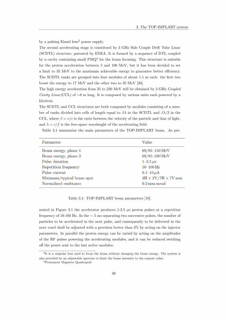
3. The TOP-IMPLART system
by a pulsing Einzel lens2 power supply.
The second accelerating stage is constitued by 3 GHz Side Couple Drift Tube Linac
(SCDTL) structure, patented by ENEA. It is formed by a sequence of DTL coupled
by a cavity containing small PMQ3 for the beam focusing. This structure is suitable
for the proton acceleration between 5 and 100 MeV, but it has been decided to set
a limit to 35 MeV to the maximum achievable energy to guarantee better efficiency.
The SCDTL tanks are grouped into four modules of about 1.1 m each: the first two
boost the energy to 17 MeV and the other two to 35 MeV [20].
The high energy acceleration from 35 to 230 MeV will be obtained by 3 GHz Coupled
Cavity Linac(CCL) of ∼8 m long. It is composed by various units each powered by a
klystron.
The SCDTL and CCL structures are both composed by modules consisting of a num-
ber of tanks divided into cells of length equal to βλ in the SCDTL and βλ/2 in the
CCL, where β = v/c is the ratio between the velocity of the particle and that of light,
and λ = c/f is the free-space wavelenght of the accelerating field.
Table 3.1 summarize the main parameters of the TOP-IMPLART beam. As pre-
Table 3.1: TOP-IMPLART beam parameters [19].
sented in Figure 3.1 the accelerator produces 1-3.5 µs proton pulses at a repetition
frequency of 10-100 Hz. In the ∼ 5 ms separating two successive pulses, the number of
particles to be accelerated in the next pulse, and consequently to be delivered in the
next voxel shall be adjusted with a precision better than 3% by acting on the injector
parameters. In parallel the proton energy can be varied by acting on the amplitudes
of the RF pulses powering the accelerating modules, and it can be reduced swiching
off the power sent to the last active modules.
2It is a unipolar lens used to focus the beam without changing the beam energy. The system is
also provided by an adjustable aperture to limit the beam intensity to the request value.3Permanent Magnetic Quadrupole
49
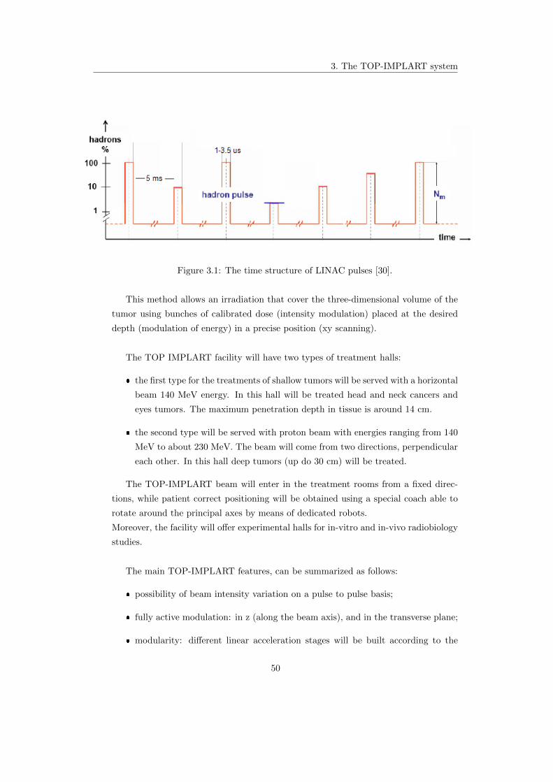
3. The TOP-IMPLART system
Figure 3.1: The time structure of LINAC pulses [30].
This method allows an irradiation that cover the three-dimensional volume of the
tumor using bunches of calibrated dose (intensity modulation) placed at the desired
depth (modulation of energy) in a precise position (xy scanning).
The TOP IMPLART facility will have two types of treatment halls:
the first type for the treatments of shallow tumors will be served with a horizontal
beam 140 MeV energy. In this hall will be treated head and neck cancers and
eyes tumors. The maximum penetration depth in tissue is around 14 cm.
the second type will be served with proton beam with energies ranging from 140
MeV to about 230 MeV. The beam will come from two directions, perpendicular
each other. In this hall deep tumors (up do 30 cm) will be treated.
The TOP-IMPLART beam will enter in the treatment rooms from a fixed direc-
tions, while patient correct positioning will be obtained using a special coach able to
rotate around the principal axes by means of dedicated robots.
Moreover, the facility will offer experimental halls for in-vitro and in-vivo radiobiology
studies.
The main TOP-IMPLART features, can be summarized as follows:
possibility of beam intensity variation on a pulse to pulse basis;
fully active modulation: in z (along the beam axis), and in the transverse plane;
modularity: different linear acceleration stages will be built according to the
50
3. The TOP-IMPLART system
financial flux and at the same time the modules already installed will be opera-
tional.
3.2 Beam monitoring
The innovative LINAC, provides a pulsed proton beam with energy and intensity
variable on pulse to pulse basis, accordingly to the requirements of the treatment.
These beam features are suitable for a fully active 3+1D dose delivery, for a more con-
formational irradiation of the tumor, even to achieve better organ motion distribution.
In fact the energy modulation permits to achieve a longitudinal scan of the tumor by
varying the depth of penetration. The lateral scan instead is obtained by deflecting
the beam in the X-Y plane. Finally the intensity modulation is necessary to a properly
dose distribution.
In addition to these, have to be considered the good ballistic properties of protons:
they realease a great amount of energy at the end of their range, causing a lot of
ionizazion events in the narrow Bragg peak region.
All these features, if optimally exploited, allow the release of high and selective dose
to the tumor area. But any deviation of the beam parameters from the planned values
may cause serious damage to the healthy tissue surrounding the tumor mass.
For these reasons the TOP-IMPLART beam requires, in particular, an accurate mon-
itor of the relevant beam parameters, on a pulse to pulse basis, which has to verify
the “exact” correspondence between the delivered dose and the dose prescribed by the
treatment plan, with an uncertainty which must be contained within a few percent.
The detector must provide, in real time, the direct measure of the X and Y beam
intensity profile, the beam direction and the spot position (centroid). The value of
the collected charge gives, then, an indirect estimation of the delivered dose. It is,
therefore, necessary to operate with a system with a high sensitivity in charge detec-
tion (10-100 fC) and able to work in a wide dynamic range (104 − 105), in order to
discriminate the signal from the instrumental background and and to span the entire
range of intensities of the beam, respectively. The precision in the measures of the
centroid position and the beam profile require a detector with a high spatial resolution
∼ 0.1 mm (about 1/10 of the minimum diameter expected for the beam cross section).
Also a prompt response (< 1 ms) is necessary to obtain an online monitor of a single
pulse and zero, or near to zero, dead time is preferable.
Like any good measurement systems, all the instrumentation used in the charge col-
lection should interfere and alter as little as possible the beam characteristics, so it
has to be built with light materials.
Furthermore any dose delivery system of this kind shall interface the accelerator control
51

3. The TOP-IMPLART system
system to correct the beam parameters or shutdown the beam if any of the measured
(or estimated) parameter is off the planned value or outside the acceptance limit re-
spectively.
Spatial resolution 0.1 mm
Dynamic range > 104
Sensitivity 10-100 fC
Dead time ∼0
Response time <1 ms
Table 3.2: Dose delivery monitor specifications.
In the next paragraph we will describe the dose delivery monitor that has been
chosen for the TOP-IMPLART beam, which is expected to satisfy all the requisites
mentioned above (Table 3.2).
3.2.1 The Pad-Strip Ionization chamber and its prototype
To best meet all requirements of a good dose delivery system, for the TOP-
IMPLART facility has been developed a monitoring system based on four indepen-
dent transmission ionization chambers. The main components of these chambers and
their geometry will be the same, but they have quite different functions: the first two
are devoted to measure the integral charge released by the beam; the other two have
segmented readout planes, for the independent reading of the charge collected in two
different directions.
Each chamber will have an active area of ∼ 30× 30 cm2. It consists of two planes, the
anode and the cathode (Figure 3.2), separated by a 2 mm gas filled gap.
The chatode is realized with a 5 µm thick Aluminium foil fixed on a Mylar layer.
For the two segmented chambers, the anode design exploits the recent developments
in Micro Patterns Gaseous Detectors (MPGD) technology. It is constitued by a 50 µm
thick Kapton foil covered, on both sides, with thin layers of Copper (15 µm) engraved
to obtain pads. On the layer exposed to the electrons, half of the pads are connected
horizontally to create horizontal strips. The other half of the pads have conductive
through-holes that permit to connect them on vertical direction, by copper strip on the
external side of the anode (Figure 3.3). Ultimately, the ionization electrons collected
on the anode are readout by strips along X and Y. The pad-like design is a technical
solution to permit the through-holes and at the same time guarantee the same effective
collecting areas for X and Y strips. In this way, it is possible the independent reading,
52
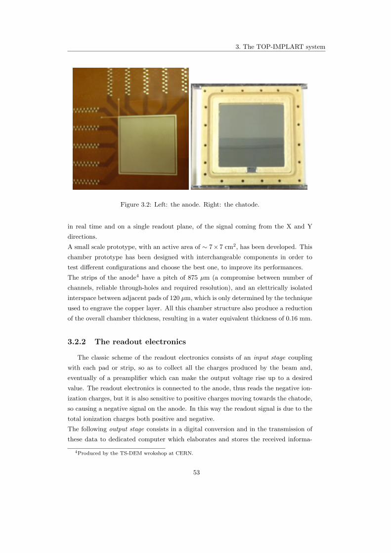
3. The TOP-IMPLART system
Figure 3.2: Left: the anode. Right: the chatode.
in real time and on a single readout plane, of the signal coming from the X and Y
directions.
A small scale prototype, with an active area of ∼ 7× 7 cm2, has been developed. This
chamber prototype has been designed with interchangeable components in order to
test different configurations and choose the best one, to improve its performances.
The strips of the anode4 have a pitch of 875 µm (a compromise between number of
channels, reliable through-holes and required resolution), and an elettrically isolated
interspace between adjacent pads of 120 µm, which is only determined by the technique
used to engrave the copper layer. All this chamber structure also produce a reduction
of the overall chamber thickness, resulting in a water equivalent thickness of 0.16 mm.
3.2.2 The readout electronics
The classic scheme of the readout electronics consists of an input stage coupling
with each pad or strip, so as to collect all the charges produced by the beam and,
eventually of a preamplifier which can make the output voltage rise up to a desired
value. The readout electronics is connected to the anode, thus reads the negative ion-
ization charges, but it is also sensitive to positive charges moving towards the chatode,
so causing a negative signal on the anode. In this way the readout signal is due to the
total ionization charges both positive and negative.
The following output stage consists in a digital conversion and in the transmission of
these data to dedicated computer which elaborates and stores the received informa-
4Produced by the TS-DEM wrokshop at CERN.
53

3. The TOP-IMPLART system
Figure 3.3: Front and back structure of the anode layout (not in scale) [28]. Left: pad-
like structure, on the exposed side, connected orizzontally; Right: the vertical strips
and the through-holes on the external side of the anode that connect the pad-like
structure on the opposite side.
tions. In existing clinical beam monitoring using ionization chambers, the readout is
based on the rateometer [22]: this device collects charge from the detector and transfers
it to the capacitor of the operational amplifier that operates the charge-voltage con-
version. A discriminator, in the following stage, compares the voltage reached in the
capacitor to a predefined value (V in the Figure 3.4). When the threshold is reached,
the one-shot pulse generator emits a signal towards the scaler, while, enabling at the
same time, the complete discharge of the capacitor. The emitted signal is counted by
the scaler. The system sensitivity is given by the quantum voltage V that has been
chosen while the system dynamic is given by the maximum number of pulses that this
device can generate during charge collection time. The rateometers works excellently
well in continuous or “long” pulsed beam, but not for fast and short pulsed LINAC; in
fact as discussed above and summarized in Table 3.1, the TOP dose delivery monitor
requires a dynamic range larger than 104 which implies, for a pulse of 10 µs, assuming
uniform charge distribution, a scaler frequency of at least 1 GHz (and corresponding
fast discharge circuit).
For these reasons, the readout system is based on a multiplexer coupling the tran-
simpedance input stage to the ADC converters. This multiplexing logic routes the
collected charges on the different channels into a single ADC input, as well as the gain
54

3. The TOP-IMPLART system
Figure 3.4: Rateometer scheme.
status informations.
In this way the dynamic is limited by the saturation of the input stage and by the
number of the sampling bits of the ADC which ranges around the value of which is
commonly available up to 16 bits. To avoid saturation in the input stage, a variable
transimpedance gain mechanism has been adopted: the gain is dynamically adjusted
depending on the collected charge. In other words the gain (i.e. the conversion factor
Q/V) diminishes as soon as the input charge exceeds a certain threshold fixed by the
maximum value of the output voltage (saturation). Using this technique it is possible
to reach a global dynamic higher than 104 with small overall costs.
A prototpye based on discrete components, has been implemented by small front-
end boards handling 16 channels each. Up to 10 boards (5 along X axis and 5 along
the Y ones) can be used in the prototype chamber, reading up to 80 channels. For the
first tests and characterization only 6 cards have been used, acquiring in this way the
48 central channels in both directions.
3.2.2.1 Input stage and adaptive gain change
The basic element of the readout front-end electronics is composed by the Burr-
Brown IVC102 chip [23], an active integrator circuit realized with an operational am-
plifier (OP-AMP). As we can see in Figure 3.5, for each channel (strip), the current
coming from the ionization chamber is integrated over the feedback capacitor C1 of
the OP-AMP. The current integration occurs when the electronic switch S1 closes and
the GATE signal is set on. The integration continues for the whole duration of the
55

3. The TOP-IMPLART system
GATE interval5. In this way a charge to voltage (Q/V) conversion is obtained. The
following step is the reading of the final voltage Vout and the consequent discharge of
the capacitor C1, restoring the initial condition of operation. The phase of discharge
takes place by means of the RESET signal which closes the swich S2. It is important
that the RESET signal is long enough to guarantee that the capacitor has been totally
discharged (with a maximum residue of 0.01%) to not alter the following measurement
with the presence of residual charges.
As we have already seen, the TOP-IMPLART beam characteristics require that the
beam monitor should measure the charge Q in a wide interval, over four order of mag-
nitude, with a 5% of maximum error. Furthermore, another limit is imposed by the
ADC which sets the maximum value of Vout, the voltage in output from the integrator
stage and in input for the ADC, to Vthr = 10 V. Also, the high sensitivity requires
that the integration occurs on a small capacitance, but at the same time if a great
charge is present, saturation problems have to be avoided, through the integration on
a bigger capacitor.
For all these reasons a dinamically electronic system has been designed, with the main
feature of automatically adjusts its dynamic range by diminishing the charge to voltage
conversion factor. This automatic gain change occurs when the output voltage Vout
rises near the maximum value allowed by the ADC (10 V): the Vout signal is compared
to the threshold voltage by a discriminator circuit and if results Vout > Vthr a second
capacitance C2, in parallel to the first one, is set on. When Vout exeeds the threshold
value a bit of information is sent to the LATCH 6, which in turn closes the S3 that
enables the capacitance C2. In the new configuration two different things occur:
The dynamic range of the system increases, making possible to correctly scale
the Vout value and to calculate the right collected charge Q;
The gain of the trans-amplifier Q/Ctot decreases, due to the increase of the total
capacitance Ctot = C1 + C2.
The Vout trend is shown in Figure 3.6 . These signals have been obtained in labora-
tory using a battery as source of current (instead of the chamber). The GATE signal
has been generated by a function generator system. From the figure it is clear that,
when the additional capacity is inserted, an abrupt discontinuity occurrs in the Vout
trend, due to the charge distribution between the two capacitors. Then, Vout restarts
to increase, with less gain, until the GATE signal is on. At the end of the GATE,
5During the time the swich S1 is open, the charges accumulate in the ionization chamber, as soon
as the switch closes, it is transfered to the capacitance C1, avoiding charges losses and reducing the
dead time to zero.6This circuit latches the input transition as long as it is reset.
56

3. The TOP-IMPLART system
Figure 3.5: Electronic scheme of the input stage with multi gain amplification logic
[27].
57

3. The TOP-IMPLART system
after a short transition, the voltage value stays costant: this is the correct value will
be converted from the ADC.
When C2 is inserted the redistribution of the charges can cause a damping oscillation
in the signal (Figure 3.7) that might alter the measure, the oscillation can be mini-
mized by the insertion of the tuning resistor RTUNING.
Figure 3.6: The output signal of the input stage: the discontinuity indicates the gain
change and the costant Vout at the end of GATE represents the voltage value will be
converted from the ADC.
Figure 3.7: Output signal of the input stage before compensation (left) and after
compensation (right) [26].
Figure 3.8 shows a picture of the chamber and the electronics boards, inside the
shielding box. The beam hits the anode represented in the bottom left part of the
figure. The six electronic cards are clearly visible. A single card structure is presented
58

3. The TOP-IMPLART system
in Figure 3.9 .
Figure 3.8: View of the whole prototype pad-strip ionization chamber.
Figure 3.9: A electronic card used for the readout of the chamber signal.
59

Chapter 4
Test and Calibration of the
monitor chamber
The TOP-IMPLART LINAC has recently delivered its first 27 MeV energy proton
beam. This energy is high enough to permit an extensive test and characterization of
the chamber prototype; in fact the range of 27 MeV protons in water is ∼ 0.75 cm and
they release ‘only’ < 2% of their energy in the chamber: it can be considered a ‘small’
perturbation.
In these conditions, systematic measurements are ongoing to study the chamber re-
sponse and define the proper characterization procedure, in clinical-like conditions. In
particular, the chamber prototype as been tested to:
determine the operating point of the chamber;
equalize the channels response;
study the chamber adaptive gain mechanism and calibrate it;
evaluate the charge to dose calibration factors.
4.1 Experimental setup
The detector has been installed on a mobile support, which allows the movement
of the chamber along the beam line. Also the transverse position with respect to the
beam can be varied, thanks to two orthogonals arms that can be moved by step-motors
remotely controlled. Before starting each irradiation cycle the suitable distance dair
from the beam pipe exit window1 has been chosen and the chamber has been correctly
1approximately it can be assumed that the beam divergence starts from the beam pipe exit window.
60

4. Test and Calibration of the monitor chamber
aligned with the beam pipe with the help of two laser systems, indicating the center
of the beam spot on each side of the chamber.
For all the tests the ionization chamber was filled with air at atmospheric pressure.
It is worth mentioning that the presence of Oxygen in air reduce the charge collec-
tion efficiency, due to the attachment and recombination mechanisms, as described in
Section 2.3.1.1. But, on the other hand, the use of air as filling gas greatly simplifies
the acquisition procedure, avoiding problems connected to the presence of other gas
mixtures.
The bias voltage of the detector has been supplied by the CAEN High Voltage Power
Supply Module DT1419ET, which can provide a ±500 V maximum voltage (with an
accuracy of 1%) and a 200 µA maximum current. The voltage have been set by remote
host PC using the software GECO2020 distributed by CAEN.
The acquisition system is composed by:
the front-end electronics described above (Section 3.2.2).
VMIC VMIVME-7697 Pentium III Processor based VMEbus CPU; it runs the
acquisition program (developed in C) that control the VME modules and store
the data acquired from the ADC.
VMIC VMIVME-3120 (8 MHz- 12 bit) Analog to Digital Converter board; it
converts the Vout multiplexed values coming from the front-end electronics and
acquires the information on the gain status of each channel, pulse by pulse.
CAEN V770 Input/Output Register; it provides the logic signals to the front-
end electronics (GATE, CLEAR/RESET, CLOCK for multiplexing ...) and the
synchronization signal to the accelerator.
CES VMDIS 8004 a VME display and diagnostic module; it is used during the
acquisition as a Interrupt generator on the VME bus, triggered by the end of an
accelerator pulse.
The lenght of the GATE signal and the acquisition rate are configurable parame-
tres in the acquisition software. The GATE width can be varied considering that it
has to be large enough to permit the integration of the whole collected charge. The
acquisition rate f , which can achieve the maximum value of f = 250 Hz, coincides
with the beam pulse rate. In fact, in all tests the monitor chamber acts as trigger
source for the single beam pulse and the chamber electronics is synchronized to the
passage of the beam. This condition on one side “simulate” the clinical behaviour of
the dose delivery monitor that shall authorize the delivery of the single beam pulse
and on the other somehow simplify the measurements; however, in the final version the
61

4. Test and Calibration of the monitor chamber
chamber electronics will operate asynchrounsly to the beam, though it will continue
to authorize the beam pulse delivery.
4.2 Preliminary considerations
Some definitions and notations should be introduced before going through the
discussions of the different measurements:
Event e is a single reading cycle, which coincides with a beam pulse.
Run indicates the period in which the conditions of the beam and the chamber
are expected to be stable; each run is composed of series of beam pulses.
Di(e) is the ADC value obtained from the channel i at the event e.
gi(e) indicates the particular configuration of the electronic channel i during the
acquisition of the event e. Essentially it corresponds to the configuration of the
feedback capacitors2 of the transimpedance circuit which determine the gain. We
define g0i e g1
i the gain values in the basic configuration and in the gain-changed
configuration respectively.
Qi(e) represents, for each channel and event, the charge collected on the feedback
capacitances: the quantity we would measure, since it corresponds to the ioniza-
tion charge released by the proton beam passing the chamber active volume and
therefore proportional to the charge of the beam.
Ci(e) stays for the value of the feedback capacitors; it depends on the gain
configuration and it can vary for each event during the run, due to the adaptive
gain of the electronics.
Vi(e) is the ouput voltage measured at the exit of the transimpedance OP-AMP
(Section 3.2.2.1).
The goal is to measure, for each event, the amount of charge released by the beam
in the ionization chamber and then collected on the feedback capacitors. This can be
achieved in two steps. First, extrapolating the ADC values Di(e) for each pulse and
channel; then converting them into voltage values Vi(e). The conversion factor fV can
be estimated by the ratio between the input dynamic of the ADC (20 V in our case)
and its maximum bin number (4096). Hence fV = 204096 V. In our prototype detector,
2The stauts of the feedback capacitors configuration is provided for each event by the LATCH bit,
as discussed in Section 3.2.2.1
62

4. Test and Calibration of the monitor chamber
fV would not depende from the electronic channel because the output of each channel
is multiplexed to a single ADC converter.
The correct voltage at the terms of the feedback capacitances of the OP-AMP results:
Vi(e) = fV · [Di(e)−Dpi (gi)] (4.1)
where Dpi (gi) represents the pedestal, i.e. the ADC value recorded in absence of signal,
for the channel i in the gi configuration.
This voltage, in turn, results proportional to the collected charge on the capacities
Vi(e) = Qi(e)/Ci(e)
so inverting and using the equation 4.1 the charge is obtained by:
Qi(e) = gi(e) · [Di(e)−Dpi (gi)] (4.2)
With the substitution gi(e) = fV · Ci(e).
The error on Qi(e) depends essentially on the uncertainties on gi and on Di(e).
gi is estimated from the electronics implementation and is assumed to be “exact”; it
may assume two values for each channel, and its error is essentially systematic, and
expected to be small. The main source of error is therefore the measurement of Di(e),
which can be estimated by the RMS of the pedestal of each channel: this value is
pretty small (at the level of few ADC units maximum) on a scale of about 2000 ADC
units. However, the simple pedestal does not account (and cannot be easily estimated
with the current version of the electronics) for the potential perturbation that can
be induced on the collected charge by the logic transitions due to the adaptive gain
mechanism. Moreover, in the measurements presented in the next sections, the largest
contribution to the statistical fluctuation of Di comes from the beam pulse-to-pulse
variability.
4.3 Ionization regime
To determine the operating point of the chamber, a set of runs has been performed
varying the supply voltage of the detector and leaving the other parameters unchanged.
The ionization chamber was positioned at a distance in air from the beam pipe exit
window dair = 84 cm. The beam intensity was kept nearly costant by maintaining
stable the value of the Einzel lens at 28.2 kV.
The voltage has been varied in the range 0 ≤ HV ≤ 450 V in steps of 50 V.
The goal of this scan is to estabilish the voltage range in which the detector operates
63

4. Test and Calibration of the monitor chamber
in the ionization regime, i.e. when the response of the chamber remain constant inde-
pendently from the voltage supply.
For each of these runs the integral charge collected from the chamber has been calcu-
lated, by summing for each active channel the charge deposited in each pulse. This
procedure has been adopted for the calculation of the total charge collected along both
X and Y axes. The total charge collected from the whole chamber is obtained by sum-
ming the values of charge along X and Y directions. These integral charge values are
plotted in Figure 4.1 as a function of the respective supply voltage. From this figure
it is clear that the plateau region is reached between 250 V and 450 V: in this interval
the chamber is expected to operate in the ionization regime. In fact, if the voltage
applied is too low some of the electrons recombine with positive charges, as mentioned
in Section 2.3.1.1, and do not reach the anode surface. For higher voltage, above the
ionization regime, the chamber enters in the proportional regime where, the generally
large beam intensity may cause saturation.
Figure 4.1: X, Y and total collected charge as a function of the applied high voltage.
4.4 Tests of operation
4.4.1 Pedestal
As we have already seen, to correctly calculate the charge values, pedestals shall
be estimated and subtracted to the ADC data. Pedestals represent the signal recorded
by the ADC when no beam is present and therefore give information on the chamber
response noise, by the evaluation of the RMS of the pedestals. The pedestal acquisition
tipically occurs immediately before the beam acquisition, in the same conditions the
beam will be acquired (gate width, frequency, gain, environmental conditions).
The peculiar time structure of the TOP-IMPLART beam, with beam pulses which
64

4. Test and Calibration of the monitor chamber
follow one another after few milliseconds, permits the pedestal acquisition in the same
run of the measurement. In particular, the pedestal data can be acquired in the period
between two successive pulses, when the beam is off. So, at first, we obtain an ADC
pedestal value for each beam pulse and channel. After it is estimated for each channel
as the average value on all run pulses.
Dpi (gi) =
∑eDi(e; gi)∑
e 1
This value should be independent, or weakly dependent, from time and then from the
pulse.
In Figure 4.2 the the pedestals are reported as a function of the electronic channel.
Figure 4.2: ADC Pedestal as a function of all the electronic channels.
An analysis of the pedestal values and therefore of the noise, in the gain basic
configuration, has been performed as a function of the gate width and the detector
supply voltage. The chamber was positioned at dair =26 cm from the beam pipe
window. Five different runs have been taken varying the gate width, each for two
values of the bias voltage. For each run the mean pedestal values has been calculated,
averaging on the ADC pedestals obtained for each ADC channel i. The data are
plotted in Figures 4.3 and 4.4. The error bars assigned to the pedestal values, not
visible in the plots, were obtained as the standard error on the mean.
The results suggest that:
65

4. Test and Calibration of the monitor chamber
For fixed GATE width, the voltage variation does not alter the pedestal values:
the maximum variation on the data is ∼ 0.001%;
For fixed bias voltage, the trend of the pedestal values slightly increase with the
GATE duration: the maximum variation on the data recorded is ∼ 0.1%. This
increase can be due to the drift motion of the charges in the detector.
Figure 4.3: Pedestal ADC at various GATE lenghts. HV=200V. Data fitted with a
second order polinomial function.
Figure 4.4: Pedestal ADC at various GATE lenghts. HV=300V. Data fitted with a
second order polinomial function.
The above discussion is limited to the pedestals of the base gain configuration of
the electronics, i.e. when only one feedback capacitance is active. In fact, for each
channel, there are as many pedestals as the number of adaptive gains, that in the
current implementation are 2. The second gain pedestals are discussed in Section 4.5.
66

4. Test and Calibration of the monitor chamber
4.4.2 Channels equalization procedure
From the values of collected charge in each strip, the X and Y beam profiles have
been obtained as the mean, over all the pulses of the run and for each channel i, of the
collected charge as a function of the strip number. The typical beam profile should
be nearly a Gaussian with a mean value corresponding to the center of the beam spot
with respect to the detector reference system, and the width3 which is larger for larger
chamber-beam pipe distances.
The analysis of some of these beam profiles has highlighted that the charge profile
is not exactly fitted by a gaussian function due to small, uncompensated, systematic
fluctuations of the single strip response, as shown in Figure 4.5.
Figure 4.5: Y beam profile. Run parameters: HV = 200 V, dair = 75 cm. The
parameter p0 corresponds to the amplitude of the Gaussian, p1 is the mean value, p2
the sigma, p3 and p4 the offset and the slope of the linear baseline.
The fluctuations have been compensated by the following, pretty standard, pro-
cedure. A reference run is taken putting the detector far away from the beam pipe
(dair = 100 cm) so that the beam would invest the entire sensitive area of the detector,
resulting in a nearly flat beam profile for each X and Y directions (Figures 4.6).
3The width on each axis is measured either as the Gaussian σ or as the Full Width at Half
Maximum of the profile FWHM = 2σ√
ln 2.
67

4. Test and Calibration of the monitor chamber
Figure 4.6: X and Y beam profiles used as reference for the equalization procedure.
Run parameters: HV = 200 V, dair = 100 cm, E. Lens 30 kV .
The profiles have been fitted with a Gaussian function (plus a linear baseline).
Then, an equalization factor Hi has been associated to each channel. This factors
have been calculated from the relation:
Hi =fiki
(4.3)
where ki stands for the value of the collected charge along the ith−strip, and fi repre-
sents the Gaussian fit value corresponding to the same strip. By definition, multiplying
the strip charges of this reference run for the respective equalization factors, we find
the exact values obtained by the fit. Instead, if these factors were applied to other
runs, the correctly equalized charge values are obtained.
The goodness of this procedure was verified by applying it to runs made under different
conditions, i.e varying the geometry of the system, the supply voltage of the detector
or the beam intensity (Einzel lens). In the next figures 4.7 and 4.8, different beam
profiles are shown after being equalized.
68
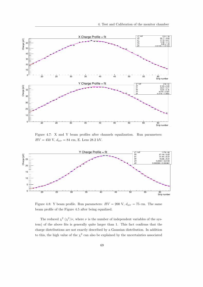
4. Test and Calibration of the monitor chamber
Figure 4.7: X and Y beam profiles after channels equalization. Run parameters:
HV = 450 V, dair = 84 cm, E. Lens 28.2 kV.
Figure 4.8: Y beam profile. Run parameters: HV = 200 V, dair = 75 cm. The same
beam profile of the Figure 4.5 after being equalized.
The reduced χ2 (χ2/ν, where ν is the number of independent variables of the sys-
tem) of the above fits is generally quite larger than 1. This fact confirms that the
charge distributions are not exactly described by a Gaussian distribution. In addition
to this, the high value of the χ2 can also be explained by the uncertainties associated
69

4. Test and Calibration of the monitor chamber
to the measurements, which are affected also by the beam fluctuations between pulses,
larger than the pulse statistical fluctuations of the mean value.
However, the channel equalization through the Gaussian fit, generally improves (re-
duces) the mean distance between the data points and the fit curve by 5-10 times
respect to the uncompensated values.
4.4.3 X/Y charge collection
Quite a few runs have been taken to study the uniformity of the X and Y strips
relative responses. Figure 4.9 reports the scatter plot of the total charge deposited on
the X strips and the Y strips. The color scale on the right represents the frequency of
each reported charge values. The trend of the plot and the correlation factor close to
1 demonstrate the strong linear correlation between the two quantities.
For the same run the ratio of the X and Y charges collected on the single pulse is
Figure 4.9: X-Y charge sharing. Run parameters: HV = 200 V, dair = 26 cm.
shown in Figure 4.10 as a function of the acquisition time, expressed in minutes. Also
the X to Y charge distribution is presented. From the graph it is clear that all the
charge ratios are higher than unity, in particular for this run, averaging on all the
pulses charges, results a X/Y mean charge ratio:
X/Y charge = (1.191± 0.005)
70

4. Test and Calibration of the monitor chamber
Figure 4.10: Left: X to Y charge ratio as a function of acquisition time. Right: X to
Y charge distribution. Run parameters: HV = 200 V, dair = 26 cm.
Figure 4.11: X to Y mean charge ratio for different run as a function of the applied
high voltage.
Repeating the measurement for other runs, the trend is the same: a charge collec-
tion slightly greater along X with respect to Y. This trend is explained by the different
collecting geometry of the strips: in fact, in the horizontal direction the pads surface
is slightly larger than the one in Y, so the charge collected by the former is greater
than that collected by the latter. Variations until 6% can occur in this charge ratio,
at different configurations of chamber-beam pipe distances which are affected by the
limited size of the chamber and then to border effects. Instead, a negligible voltage
dependence is clearly visible in Figure 4.11, where are shown the X/Y mean charge ra-
tios for runs performed in the same geometry but with different values of bias voltage.
71

4. Test and Calibration of the monitor chamber
The average value of the X to Y charge ratio over the measures results:
X/Y charge = (1.116± 0.009)
4.5 Automatic gain change
As mentioned above, one peculiar feature of the prototype readout system is the
multi gain amplification adaptive mechanism. Above the voltage threshold (which set
a maximum also in the ADC value, ADCthr) the feedback capacitance C2 is inserted
in parallel to the basic capacitance C1 = 10 pF of the IVC102, as described in Section
3.2.2.1.
During the run, for each channel, at least three situation can occur:
1. the channel has not undergone gain change during all the run, i.e. it always lies
below threshold;
2. the channel changes its gain automatically, in one or more of the pulses collected
during the run; i.e. the ADC value oscillates around the threshold value;
3. the channel changes its gain for all the pulses of the run; i.e the ADC value lies
always over the threshold value.
The first case represents the simplest situation: the measurement of the charge
Qi results simply from the integration on the constant capacitance C1 = 10 pF and
by the subtraction of the correct value of pedestal, we have already examined in the
Section 4.4.1. The ADC trend as a function of the collected charge is represented by a
continuous curve (Figure 4.12). The ADC values stay below the threshold value for all
the duration of the run. The gain configuration can be easily estimated as the slope
of the curve.
The second and third case, instead, are more complex. We will examine them in the
next section.
4.5.1 Gain calibration
When the ADC value overcomes the threshold the automatic gain change occurs:
the gain diminishes and the dynamic range is extended. The gain value is strictly
dependent from the value of the inserted capacitances. In order to study the behaviour
of the adaptive gain, different values of C2 capacitors have been used on different
electronic boards (same values of C2 for all channel on a single board). Also, higher
capacitance values have been chosen for the cards connected to the central strips of the
72

4. Test and Calibration of the monitor chamber
Figure 4.12: Charge collection (as ADC values), for all the channels in the basic gain
configuration, as a function of the beam intensity. Each colored line represents the
trend of a single channel.
73

4. Test and Calibration of the monitor chamber
anode, which, if the monitor is correctly aligned with the beam, has more changes to
collect a greater amount of charge respect to the lateral ones. The C2 configurations
are:
X axis:
– card 0: C2 =100 pF
– card 1: C2 =1200 pF
– card 2: C2 =470 pF
Y axis:
– card 3: C2 =220 pF
– card 4: C2 =1000 pF
– card 5: C2 =470 pF
Figure 4.13 represents, for one of the i channels, the trend of the collected charge
(as ADC values) during the run period, as a function of the beam intensity, estimated
by the sum of the charges of those channels (on the given axis) that do not change the
gain in the run. Each point in the figure represents a single beam pulse. An abrupt
Figure 4.13: Charge collection (as ADC values), for one channel, as a function of the
beam intensity. The discontinuity indicates that gain change occurred.
discontinuity occurs in the curve when the ADC reaches its maximum ADCthr, the
74

4. Test and Calibration of the monitor chamber
capacitance C2 is inserted (for the represented channel C2 =100 pF), the charges
collected divides between the two capacitors, in turns the gain diminishes and then
the charge increases again. The two gain states are clearly visible from the Figure 4.13
and they distinguishes from the different slopes of the curves, inversely proportional
to the feedback capacitances.
The nature of gap in the ADC values, between the two curves, is strictly related to
the pedestal of the second gain stage, different from the previous. The values of these
pedestals need to be calculated, to achieve a correct estimation of the collected charge.
But, the current electronics prototype cannot force the gain change to evaluate directly
the pedestal when C2 is inserted. For this reason two different methods, independent
from the electronics, have been developed.
4.5.1.1 Method 1: Channels with gain change oscillating during the run
Consider a channel state in a given run oscillates, on different pulses, between two
states of the collected charge around the ADCthr value that induce the gain change.
At each time during the run the charge results:
Qi(e) = gi(e) · [Di(e)−Dpi (gi)] (4.4)
with pedestal Dpi (gi) depending on the electronic state. When beam intensities fluctu-
ations induce gain change, we suppose, for each channel, that no charge discontinuity
occurs, in particular that the maximum value of the collected charge in the first gain
stage equals the minimum charge value reached in the second gain stage:
maxe∈g(e)=g0
Q(e) = mine∈g(e)=g1
Q(e) (4.5)
where the channel index i has been suppressed for clarity.
The maximum and minimum charge values can be espressed as equation 4.4, then
applying 4.5:
g0(e)[Dmax(e, g0)−Dp(g0)] = g1(e)[Dmin(e, g1)−Dp(g1)] (4.6)
In this way the only unknow quantity results the pedestal value after the gain change:
Dp(g1) = Dmin(e, g1)− g0
g1[Dmax(e, g0)−Dp(g0)] (4.7)
4.5.1.2 Method 2: Channels undergoing gain change in the entire run
In a condition of beam stability, a set of runs can be performed in different ex-
perimental configurations (for exemple varying HV). In this situation we can assume
75
4. Test and Calibration of the monitor chamber
the proportionality between the mean charges collected in the same channel of two
different runs r1 and r2 respectively:
Qr1i = αiQr2i
where αi is the proportionality factor for each channel i.
If the following situations occur:
each channel of r1 stays always under the threshold value;
some channels of r2 are always under the threshold value and others always
exceed that value;
then is possible to estimate the mean charge in r2 as:
〈Qr2i 〉1 =〈Qr1i 〉0α
where α is taken costant for each channel and is calculated as a mean running on only
the channel that are always in the base gain configuration:
α =
∑iQ
r1i /Q
r2i∑
i 1
At this point, it has been obtained an estimation of Qi in the second gain stage,
so by the substitution of the charge expressions:
g1i ·(〈Dr2
i 〉1 − 〈Dpi (g1
i )〉1)
=g0i
α· 〈Dr1
i −Dpi (g0
i )〉0
By inverting this formula is possible to achieve an estimation of Dpi (g1
i ):
Dpi (g1
i ) = 〈Dr2i 〉1 −
g0i
α · g1i
〈Dr1i −D
pi (g0
i )〉0
Both methods described above, have been tested on different data sets: pedestals,
in the gain changed regime, have been calulated and then subtracted to the ADC
values for the correct charges values estimation.
However, the results are still not satisfactory for all the detector channels. From a
more accurate analysis of each channel behavior, it has been found that some of these
behave in an incosistent way with respect to the gain change mechanism. For exemple,
in Figure 4.14 the ADC trend of a badly working channel is shown: after the ADC
discontinuity, due to the insertion of the second capacitance, the gain seems to decrease
rather than increase. The reason of this odd behavior is now under study; probably, it
may be due to problems associated to the electronics of these channels, e.g. unwanted
charge loss on the capacitors C2 due to draining of the inserted switch.
76

4. Test and Calibration of the monitor chamber
Figure 4.14: Charge collection (as ADC values), for one channel, as a function of the
beam intensity. The discontinuity indicates that gain change occurred. The negative
slope of the second gain stage evinces an anomalous trend in the charge collection.
4.6 Dose measurements
In the dose measurements, the response of the chamber has been compared (and cal-
ibrated) to the response of “classic” dosimeters such as Alanine pills and GaFChromic
films.
In the following, the ionization monitor chamber has been used as a sort of direct
dosimeter, estimating the dose values from the amount of collected charges. It is
worth mentioning that this is not the proper operation of the chamber: when used in
clinics the chamber charge response will be compared to the expected response esti-
mated by the treatment plan; the chamber does not really act as a dosimeter but as a
beam charge position and intensity monitor. However, to easily compare the response
of the small dosimeters (Alanine pills, films, etc ...), in conditions of not ideal geometry
for the chamber (the beam cross section is larger that the chamber active area) the
chamber has been modelled as a sort of 2D pixel detector as discussed in the following.
These not optimal operating conditions have been chosen in view of radiobiological ex-
periments on small animals, whose irradiation require their positioning at a distance
of about a meter from the beam pipe window.
It is worth mentioning that the model adopted for the dose extraction provides the
integral dose value released in each pixel of the detector, as it happens for the other
dosimeters. But, in a clinical setting, it would be useful to monitor released dose pulse
77

4. Test and Calibration of the monitor chamber
by pulse; this objective could be achieved by improving the model used for the dose
calculation and using other independent detectors. However, the good correspondence
between the integral dose values provided by the ionization chamber and by the vari-
ous dosimeters used as a reference, suggest that also the dose values issued for single
pulse could be comparable.
The main goal is to determine the precise dose, released in each pixel of the monitor,
with an accuracy better than 5%. The strip dose distribution has been obtained
rescaling the X and Y charge beam profiles into dose profiles by means of a properly
conversion factor. This conversion factor fstripdose has been estimated by the relation
2.3, with the substitution:
fstripdose =wair
vstrip · ρair(4.8)
where the following parameters have been used:
wair = 34.3 eV is the ionization potential for protons in air;
ρair = 1.204 Kgm3 is the air density at a temperature of 20C;
vstrip = 1.225 · 10−7m3 is the active volume whose ionization charge is collected
by a single strip, it is vstrip = p× l × t where:
– p=875 µm is the pitch of the strip;
– l=80× p represents the strip lenght;
– t=2 mm is the gap thickness.
Figures 4.15 and 4.16 show the X and Y strip dose profiles: the points represent
the experimental data and the red curve a Gaussian fit.
Then, for the estimation of the pixel dose distribution, the two unidimensional beam
profiles have been combined to obtain two-dimensional informations about the beam
intensity cross section. Assuming that the two X and Y charge profiles correspond to
the differential charge profile of the single strip of the orthogonal axis4, the amount
of charge qij released in the pixel ij (where the pixel ij refers to the superposition
area of the strip i along X and the strip j along Y) has been estimated weighting the
charge qi deposited along the strip i for the the charge qj deposited along the strip j
and then normalizing to the total charge collected along X and Y directions:
qij =qiqj∑
i qi +∑j qj
(4.9)
4This assumption is valid under specific hypothesis on the simmetry of the beam spot shape, which
seem to be satisfied by the TOP-IMPLART beam.
78

4. Test and Calibration of the monitor chamber
Figure 4.15: X strip dose profile and Gaussian fit. Run parameters: dair =110 cm,
HV=200 V.
Figure 4.16: Y strip dose profile and Gaussian fit. Run parameters: dair =110 cm,
HV=200 V.
79

4. Test and Calibration of the monitor chamber
The pixel dose Dij is obtained applying the conversion factor fpixeldose:
Dij = fpixeldose · qij (4.10)
where fpixeldose is estimated as the previous case but considering the volume of a
single pixel instead of the entire strip:
vpixel = p2 · t = 1.531 · 10−9m3
In Figure 4.17 is shown the 2D dose distribution in the prototype chamber. In the
axis are reported the total strip numbers, 80 for each direction, instead the color scale
gives an estimation of the dose value in each pixel. As we have already seen, the
prototype has been realized for the acquisition of 80+80 channels, but for these first
tests only 48+48 channels have been used. For this reason we can achieve the pixel
dose estimation only for the central area ((48× 875 µm)2) of the detector surface.
However, to obtain the whole information on the pixel dose distribution, even in the
area surrounding the central one, the Gaussian fit can be used (Figure 4.18). In fact
it gives an estimation of the absorbed dose also in the “tails” of the curve, where no
active channels are present.
Figure 4.17: Bidimensional XY pixel dose distribution. Run parameters: dair =110
cm, HV=200 V.
From the analysis of these distributions we can obtain, for each chamber pixel two
estimated values of the dose Dmpixel and Df
pixel: the former obtained directly from
the measured points and the latter from the points of Gaussian (or any other better
function) fits.
80

4. Test and Calibration of the monitor chamber
Figure 4.18: Bidimensional XY pixel dose distribution obtained by Gaussian fit. Run
parameters: dair =110 cm, HV=200 V.
In these way, the pixel dose can be compared or directly related to the dosimeter
size (of the order of 1× 1 mm2 versus the chamber pixel size of 0.875× 0.875 mm2).
However the doses estimated by the two methods generally differ by ∼ 20% at
least. The main reason for this difference in the maximum value of absorbed dose lies
in the fact that we considered different size of the detector active area. In fact, for
the calulation of Dpixel the number of channels entering in the determination of the
normalization factor are only those really acquired; instead the dose calculation by
fit takes into account a normalization factor estimated by a sum running on all the
channels (from 0 to 80).
The uncertainties associated with the dose values have been calculated as the sum of
two contributions, a systematic error and a statistical one:
∆D =√
(∆Esyst)2 + (∆Estat)2 (4.11)
The two errors entering the right side of the above expression are discussed in the next
section.
4.6.1 Dose comparison
A preliminary dosimetric comparison of the dose delivery has been performed by
the comparison between the chamber response and the response of dosimetric films or
Alanine pills, irradiated in the same conditions of the detector, to obtain the calibra-
tion coefficients.
81

4. Test and Calibration of the monitor chamber
The correlation procedure between the ionization chamber and the dosimeters mea-
surements needs a careful analysis, mainly for three reasons:
they experience a different field of irradiation, due to the different dimensions of
the chamber active area and film or pill surfaces;
the alignment of the two detectors cannot yet be achieved with extreme accuracy;
the chamber and the other detector are not in the same position. So, in the
measurements, it has to be accounted their relative distance. This can be ac-
complished by considering the solid angle Ω subtended by the detectors at the
source position that, for distances d much greater than the detectors area A
results: Ω ∼= Ad2 . The ratio of the solid angles provides a first, approximate,
correction factor of the different beam fluences.
4.6.1.1 Calibration with GaFchromic films
A first set of measurements, devoted to the calibration of the monitor chamber, has
been performed using GaFChromic films EBT3. This kind of radiochromic dosimeter
is comprised of a single active layer, nominally 27 µm thick, sited between two, 120
µm transparent polyester substrate; this simmetric structure eliminates the need for
keeping track of which side of the film is facing the radiation source. The dose response
results linear up to 4-5 Gy with an uncetainty of ∼ 1.5% both for proton and electron
beams [34].
All the acquisitions have been repeated in the same conditions:
the chamber was positioned at dair = 110 cm from the beam pipe window and
its supply voltage has been fixed at HV=200 V5;
the dosimetric film was placed, behind the monitor, in the opposite direction
respect to the beam pipe. The film was fixed on a support, made of plexiglass,
with a circular aperture (diameter 1.6 cm and thickness 0.5 cm, Figure 4.19) for
the beam collimation. The distance between the chamber and the film was 14.5
cm.
the time of irradiation was about 20 s at a pulse frequency of 10 Hz, in way to
obtain ∼200 pulses in each run. The maximum dose to be realeased during the
runs is controlled by an integral ionization chamber sited on the the beam pipe
5In these first measures of dose the voltage supply of the chamber was set slightly below the
threshold for the ionization regime, to compare the dose chamber response to that of previous mea-
surements; we know that this is not an optimal condition for the ionization chamber and, in this way,
the dose response is slightly underestimate.
82
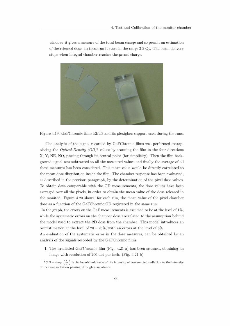
4. Test and Calibration of the monitor chamber
window: it gives a measure of the total beam charge and so permit an estimation
of the released dose. In these run it stays in the range 2-3 Gy. The beam delivery
stops when integral chamber reaches the preset charge.
Figure 4.19: GaFChromic films EBT3 and its plexiglass support used during the runs.
The analysis of the signal recorded by GaFChromic films was performed extrap-
olating the Optical Density (OD)6 values by scanning the film in the four directions
X, Y, NE, NO, passing through its central point (for simplicity). Then the film back-
ground signal was subtracted to all the measured values and finally the average of all
these measures has been considered. This mean value would be directly correlated to
the mean dose distribution inside the film. The chamber response has been evaluated,
as described in the previous paragraph, by the determination of the pixel dose values.
To obtain data comparable with the OD measurements, the dose values have been
averaged over all the pixels, in order to obtain the mean value of the dose released in
the monitor. Figure 4.20 shows, for each run, the mean value of the pixel chamber
dose as a function of the GaFChromic OD registered in the same run.
In the graph, the errors on the GaF measurements is assumed to be at the level of 1%,
while the systematic errors on the chamber dose are related to the assumption behind
the model used to extract the 2D dose from the chamber. This model introduces an
overestimation at the level of 20− 25%, with an errors at the level of 5%.
An evaluation of the systematic error in the dose measures, can be obtained by an
analysis of the signals recorded by the GaFChromic films:
1. The irradiated GaFChromic film (Fig. 4.21 a) has been scanned, obtaining an
image with resolution of 200 dot per inch. (Fig. 4.21 b);
6OD = log10(
I0I
)is the logarithmic ratio of the intensity of transmitted radiation to the intensity
of incident radiation passing through a substance.
83

4. Test and Calibration of the monitor chamber
Figure 4.20: Mean pixel chamber dose as a function of the optical density of the
GaFChromic film for different run. Run parameters (fixed in all runs): dair =110 cm,
dGaF = 125, HV=200 V.
2. The scanned image has been resampled to the ionization chamber (image of
80× 80 pixels)(Fig 4.22);
3. The resampled dose distribution is integrated along the X and Y pixels to sim-
ulate the charge collection of the X and Y strips (Fig. 4.23);
4. Then, the unidimensional X and Y strips dose distribution are combined to
obtain the 2D chamber dose distribution, as described in precedent section, both
for the experimental data and for fit data (Fig. 4.24);
5. The 2D dose distributions have been compared to the original image resampled
on the monitor chamber (Fig. 4.25).
The estimated dose is compared to the “true” resampled GaF dose by:
∆D = 2Dest −Dres
Dest +Dres(4.12)
where Dest indicates the pixel dose estimated by our method; instead Dres repre-
sents the dose values of the film resampled on the chamber. The ∆D represents the
offset, which depends on the limitation of the 2D dose extraction model. From the
color scale in Figures 4.25 can be seen that ∆D is at the level of 20− 30%, reasonably
stable, smaller for the dose extracted by the fit method, respect to the direct data
extraction. Repeating the measurements using different GaFChromic films, the mean
84
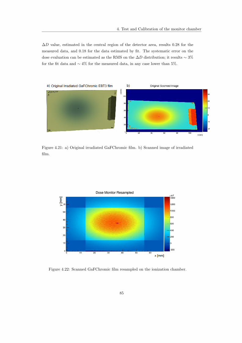
4. Test and Calibration of the monitor chamber
∆D value, estimated in the central region of the detector area, results 0.28 for the
measured data, and 0.18 for the data estimated by fit. The systematic error on the
dose evaluation can be estimated as the RMS on the ∆D distribution; it results ∼ 3%
for the fit data and ∼ 4% for the measured data, in any case lower than 5%.
Figure 4.21: a) Original irradiated GaFChromic film. b) Scanned image of irradiated
film.
Figure 4.22: Scanned GaFChromic film resampled on the ionization chamber.
85

4. Test and Calibration of the monitor chamber
Figure 4.23: Reconstructed X and Y dose profile distributions of the GaFChromic film.
Figure 4.24: 2D dose distribution for experimental data a) and for fit data b).
Figure 4.25: Comparison between the dose resampled on the monitor chamber and the
2D pixel dose distribution, both for experimental data a) and for fit data b).
86

4. Test and Calibration of the monitor chamber
4.6.1.2 Calibration with Alanine pills
An additional calibration has been performed using EPR Alanine dosimeters (Fig-
ure 4.26).
Alanine dosimeters in the form of pills are small, compact and easy to handle (diameter
4.8 mm). In these devices, the irradiation with ionizing radiation causes the produc-
tion of radicals, which number is proportional to the absorbed dose over a wide dose
range. Alanine dosimeters are characterized by low influence of temperature, humidity
and dose rate as well as a wide measuring range, which makes them applicable also for
radiation therapy. The readout of the induced signal is performed in a non-destructive
way by means of the procedure of Electron Paramagnetic Resonance (EPR). With
careful adjustment of the EPR-spectrometer and by using the appropriate dosimeters,
dose values within the range from 1Gy to 100 kGy can be determined with the overall
uncertainty 1.5− 4% [35]. The dose response results linear in the region ≤10 kGy.
For the measurements the monitor was placed at dair =84 cm from the beam pipe
Figure 4.26: Alanine pills used for irradiations.
and a plastic support for the Alanine pills was setted behind the chamber, at a relative
position of 14.5 cm.
Two types of acquisition have been performed:
1. a set of acquisitions with three Alanine pills irradiated simultaneously;
2. a set of measures with a single Alanine dosimeter.
In case 1 the pills have been sited inside the holes of the support, to form a triangle,
in order to maximize the uniformity of the dose (Figure 4.27). Various measures have
been repeated in the same configuration, varying the exposition time to the beam.
In case 2 a single pill has been housed in the central hole of the support, aligned with
the central area of the chamber. Different runs have been repeated in the same condi-
tions and at the same dose value, to evaluate the reproducibility of the measurements.
87

4. Test and Calibration of the monitor chamber
Figure 4.27: Plexiglass support for the simultaneously irradiation of three pills.
The measurements in these two configurations have been repeated for two successive
days, leaving the experimental setup and the other parameters unchanged. In Figure
4.28 the results of all the performed measurements are reported.
The trend of the chamber absorbed dose as a function of the Alanine dose is ex-
pected to be linear in the range of delivered dose (1-13 Gy), so the data have been
fitted with a linear function as shown in plot 4.28, where the different colors and mark-
ers in the plot distinguish the various configurations. The distribution of the points
suggests a deviation of the linear trend at higher dose. A more accurate analysis
highlighted that measurements performed in different days give quite different results,
probably due to beam intensities fluctuations, not included in the uncertainties asso-
ciated to the measurements. The error bar associated to the dose measurement has
been preliminary estimated to 5%7 based on the analysis of a dataset that shows a
better agreement with the linear fit; an accurate estimation of this errors need a robust
calibration procedure which is not yet consolidated enough.
Furthermore, the analisys of the measurements evinces for the ionization chamber a
maximum dose variation of 3% between the data acquired at the same nominal dose;
the variation increases for the Alanine dosimeters, reaching a maximum of ∼ 7% for the
measurements performed at nominal dose of 12 Gy. The major uniformity of response
of the chamber with respect to the Alanine can be attributed to the fact that chamber
acquisition window (GATE) and beam pulses are synchronized and some hypothetical
beam fluctuations could happen outside the GATE and therefore are not visible by
7this percentage error does not include the error arising from the model adopted for the pixel dose
estimation, discussed in the previous section.
88

4. Test and Calibration of the monitor chamber
Figure 4.28: Max pixel chamber dose as a function of Alanine absorbed dose for
different runs. Run parameters (fixed in all runs): dair =84 cm, dpill = 100, HV=200
V.
the chamber, in the current readout logic.
4.7 Preliminary beam characterization
The ultimate goal of the monitor chamber is to figure out, in real time, for each
beam pulse, deviation, of the intensity, position and direction from the values planned
for the treatment. In this directions, once the chamber has been reasonably char-
acterized by the above measurements, it has been assumed to be ready for a very
preliminary characterization of the beam.
Taking fixed the geometry of the system and the parameters of the detector, in each
run, the beam intensity has been progressively increased, by adjusting the Einzel lens
from a minimum of 24 kV to a maximum of 30 kV. The increase of beam intensity
have to correspond to an increase of the charge collected by the chamber. In Figure
4.29 is reported the trend of the single pulse charge (in arbitrary units) collected along
X and Y axes as a function of the time. Each group of point refers to the same run.
In some of the run pulse-by-pulse fluctuations (which has been induced on purpose)
of the beam are barely visible.
In Figure 4.30 the mean value of the collected charge along X and Y axes, and the
total mean charge, during all the run, are reported as a function of the beam intensity.
89

4. Test and Calibration of the monitor chamber
Figure 4.29: X and Y collected charge (in arbitrary units) as a function of the time of
irradiation, for several runs of increasing beam intensity. The value of the Einzel lens
has been increased starting from 24 kV in the first run (on the left of figures) to 30
kV in the last run (on the right of figures).
Figure 4.30: Mean collected X, Y and total charge as a function of the beam intensity
(Einzel lens). Lines connecting two successive point are for guidance.
90

4. Test and Calibration of the monitor chamber
For each pulse, it is possible to keep under control the beam parameters by a online
measure of the centroid position of the beam spot, both in X and Y directions, and its
width. The plots in Figures 4.31 and 4.33 show the trend of the centroid position, and
spot width as a function of acquisition time, on a pulse to pulse basis, for seven runs
performed at different beam intensities. Also bidimendional plots have been realized
combining the informations achieved along the two axis (Figures 4.32 and 4.34).
Figure 4.31: Beam spot centroid position, as a function of the acquisition time, for X
and Y axis.
Figure 4.32: Bidimensional distribution of the spot centroid position.
91
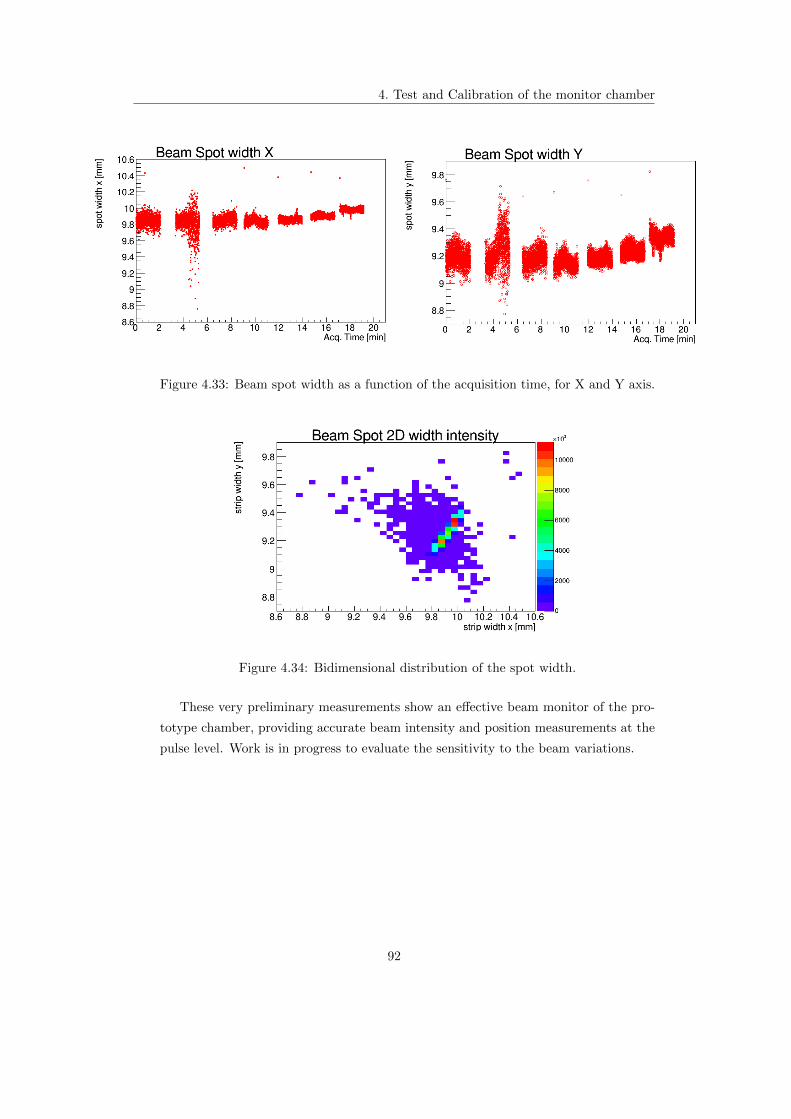
4. Test and Calibration of the monitor chamber
Figure 4.33: Beam spot width as a function of the acquisition time, for X and Y axis.
Figure 4.34: Bidimensional distribution of the spot width.
These very preliminary measurements show an effective beam monitor of the pro-
totype chamber, providing accurate beam intensity and position measurements at the
pulse level. Work is in progress to evaluate the sensitivity to the beam variations.
92

Chapter 5
Conclusions
The characteristic modular structure of a LINAC offers the possibility to exploit
the particle beam during its construction, and therefore a simpler and ongoing com-
missioning and tuning of the beam itself and of all the components of the therapeutic
system.
In this direction, the prototype of the dose delivery system for the TOP-IMPLART
LINAC, the first linear accelerator devoted to protontherapy, is under test, character-
ization and calibration, at the present beam energy of 27 MeV.
In this thesis the first proton beam measurements carried out with the Pad-Strips
ionization chamber prototype have been presented.
The preliminary results can be considered in line with the expectations. The monitor
chamber evinces an excellent correlation between the charge collected along both X
and Y directions and the adopted equalization procedure guarantees a good uniformity
in the response of each channel. These features combined with the pulsed structure of
the TOP-IMPLART proton beam, allow to monitor the beam parameters in real-time,
on single pulse basis, providing informations about the beam spot centroid position,
its width and the X and Y intensity beam profiles.
Currently, more accurate tests are underway to fully characterize the crucial mecha-
nism of the adaptive multi gain electronics. The detailed analysis has pointed out the
need to add to the electronics the possibility of pre-select the gain level to estimate
the pedestals and to evaluate the noise induced by the adaptive logic.
First attemps of dose calibration have been performed comparing the dose response
of the ionization chamber to those of conventional dosimeters: GaFChromic films and
Alanine pills. In the region of major clinical interest (1-3 Gy), the chamber dose re-
sponse is essentially linear. At higher dose values, for the same nominal dose delivered
by the beam, the chamber measures an apparent better stability (∼ 3%) respect to
93

5. Conclusions
the Alanine dosimeters (∼ 7%). This dosimetric discrepancy, assuming the Alanine
is more reliable, could be explained by the specific synchronization timing between
chamber electronics and beam pulses that may in principle prevent the chamber to be
100% dead time free.
The next developments involve the construction of a second chamber prototype, for an
independent monitor of the beam. Moreover, a new electronic version, more compact,
with larger number of channels and some additional control (as mentioned above) is
under finalization.
94

Appendix
Integral chamber
Two of the ionization chambers which constitute the monitor of the dose delivery
system for the TOP-IMPLART facility, are devoted to the direct measurement of the
integral charge released by the beam.
The structure and geometry of these integral chambers will be the same of that de-
scribed in Chapter 3, except for the anode readout plane. In fact the measure of the
total collected charge does not necessarily require a segmented readout plane, with
lots of independent channels, but this measure can be achieved simply by reading the
signal from a single channel which contains all the informations about the charge re-
leased in the whole chamber.
During each run, this monitor would be fixed soon after the beam pipe window, so in
real time will provide a direct measurement of the total charge released in the entire
irradiation period and the number of pulses in which this charge has been collected.
In this way it is possible to achieve the beam control, setting the maximum value of
charge necessary to obtain a certain amount of dose, to automatically stop the beam
when this value has been reached.
A prototype has been realized. The anode and chatode (Figure 5.1) are both realized
by aluminized Mylar foils, with active areas of 4.2 × 4.2mm2, divided by a 2 mm air
filled gap. The chamber is powered by a EMCO voltage generator, with a voltage
supply of 200 V. Charge integration can occurs on three different capacitance values
C0 = 10 pF, C1 = 30 pF and C2 = 60 pF, with a maximum value of Ctot = 100 pF if
all will be connected in parallel.
Before using this ionization chamber as beam monitor, its mode of operation has
been tested in laboratory. The signal was provided by a circuit composed by a battery
(Vbatt = 0.33 V) connected in series to a resistor and was integrated for the entire
during of the GATE signal (30 µs), provided by a function generator.
95
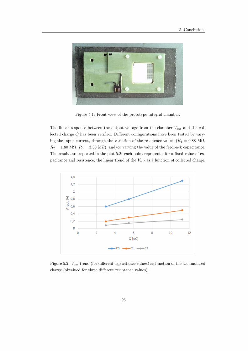
5. Conclusions
Figure 5.1: Front view of the prototype integral chamber.
The linear response between the output voltage from the chamber Vout and the col-
lected charge Q has been verified. Different configurations have been tested by vary-
ing the input current, through the variation of the resistence values (R1 = 0.88 MΩ,
R2 = 1.80 MΩ, R3 = 3.30 MΩ), and/or varying the value of the feedback capacitance.
The results are reported in the plot 5.2: each point represents, for a fixed value of ca-
pacitance and resistence, the linear trend of the Vout as a function of collected charge.
Figure 5.2: Vout trend (for different capacitance values) as function of the accumulated
charge (obtained for three different resintance values).
96

Addendum: further dose
measurements and
intercomparison
After the formal completion of the thesis work, new and more extended dose inter-
comparison measurements have been carried on using the ionization chamber, Alanine
pills (as reference), four MOSFETs, a Silicon Diode and a new Thermo Luminescent
Dosimeter based on LiF.
In fact, as explained in Section 4.6.1.2 the dose estimated by the ionization chamber
showed a surprising better stability respect to the Alanine dosimeters, which requires
further investigations, carried on by a series of new measurements, whose first and
preliminary results are summarized in the present section.
All the acquisitions have been repeated in the same experimental conditions:
the ionization chamber was placed at dIC = 95 cm from the beam pipe exit
window and the bias voltage has been kept fixed to HV=200 V;
the other dosimetric systems (Solid Dosimeters) have been sited at a distance
of dSD = 14.3 cm behind the chamber, fixed on a plexiglass support in the
configuration shown in Figure 5.3;
temperature has been monitored and remained constant within 2C.
Some corrections have been applied to the data from the ionization chamber, in
order to have dose values as much as possible consistent with those of the reference
dosimeters. These corrections involve:
1. the dose overestimation caused by the model adopted for the pixel dose extrac-
tion;
97

5. Conclusions
Figure 5.3: Dosimeters configuration: Alanine pills have been housed in the three
central circles and just above them is placed the TLD (black point); the Silicon diode
has been fixed in the lower left; three MOSFET (black strings) have been placed in the
three free corners of the support, and another one has been fixed in an almost central
position (MOSFET-giallo).
2. the different fluence of the beam on the surfaces of the ionization chamber and
the other dosimeters which sits at different distance from the beam pipe exit
window;
3. the difference in the beam energy absorbtion, due to the different composition of
each detector; the absorbed dose shall be reported to the dose-to-water (which
acts as a reference).
The first item has been discussed in Section 4.6.1.1 and can be corrected, for the
maximum dose value, applying a dose normalization factor fn to the dose extracted
by the model:
Dres = Dest · fn (5.1)
where fn derives from the Equation 4.12:
fn =2−∆D
2 + ∆D(5.2)
Which provides fn = 0.835 for fit data and fn = 0.754 without fit.
The correction factor that takes into account the relative distance can be estimated
assuming that the beam spot is pointlike at the beam pipe exit window (the source
of the beam) and the spot solid angle Ω subtended from the above point source is
constant. With this approximations the beam spot size is proportional to 1d2 , where
d is the distance from the point source. The fluence correction factor fΩ is barely the
98

5. Conclusions
ratio of the distances of the two detectors that are considered:
fΩ =d2IC
d2SD
= 0.755 (5.3)
The third correction has to be taken into account because the dose values obtained
from the Alanine (and the other) dosimeters refer to dose-to-water, instead the ion-
izazion chamber is filled with air. In this way the energy lost, by a ∼ 25 MeV proton
traversing 2 mm air filled gap, has to be rescaled to energy lost in water. The scale
factor fw can be obtained from the proton stopping powers both in air and in water,
the density of the materials and their thickness. It results in fwater = 1.136.
This estimation is based on at least two important approximations: the stopping
power in the reference dosimeters does not change noticeably (that is the Bragg Peak
is beyond the dosimeter) and the beam is composed of monochromatic protons1.
Figure 5.4 reports the whole dose data2 recorded by the IC and Alanine pills simul-
taneously corrected by the three effects descrived above. The linear fit is applied to all
points but it clearly privileges the points at lower dose, which have smaller absolute
errors. The two sets of data seems to require different calibration factors; possible
sources of this discrepancy could be the validity of the approximations used in the es-
timation of the correction factors, potential medium term instability of the ionization
chamber and misalignment effects not included in the analysis. However this analysis
evinces for the new measurements a better stability in the detectors dose response: for
the same nominal dose, only 1% variations for the IC dose and less than 2% for the
Alanine pills.
The corrected chamber dose values of the new measurements have been divided for
the Alanine dose values to obtain the ionization chamber calibration factors. These
ratios are expected to remain constant for each measurement carried out in the same
experimental conditions. In Figure 5.5 the calibration factors are reported as a func-
tion of the respective run number. The figure also shows the mean value (red line)
and a dashed band corresponding to ±1σ of the mean.
Comparison measurements were also carried out with MOSFET (Metal Oxide
Semiconductor Field Effect Transistor) and Silicon Diode dosimeters. The MOSFET
devices are composed of a doped semiconductor material substrate, usually Silicon.
The sensitive region is the gate terminal, constitued conventionally by a layer of sil-
icon dioxide. The incident radiation creates defects (acts like electron-hole pairs) in
1In fact the TOP-IMPLART beam is still characterized by significant lower energy components
which will be removed at higher energies.2The data reported in the plot are both those presented in Section 4.6.1.2 and those relative to
the new measurements.
99
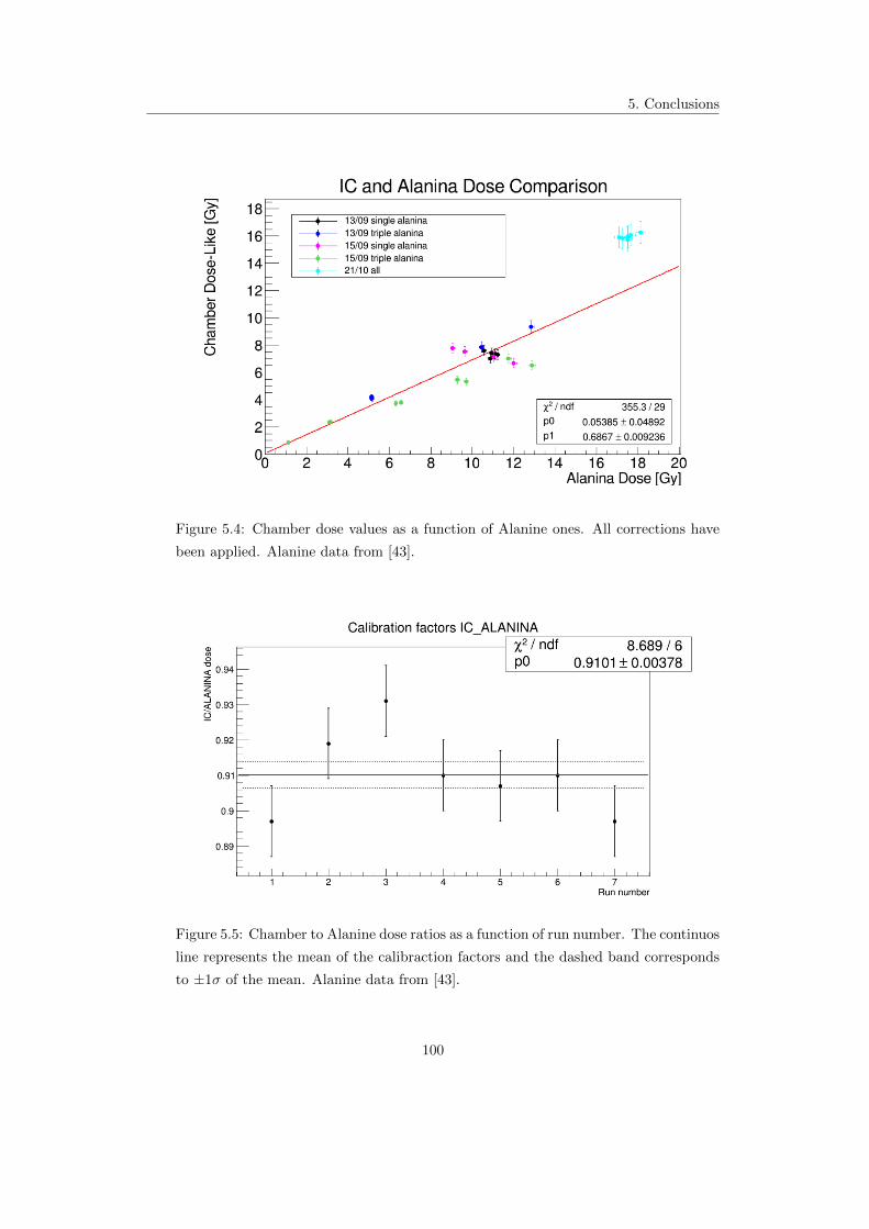
5. Conclusions
Figure 5.4: Chamber dose values as a function of Alanine ones. All corrections have
been applied. Alanine data from [43].
Figure 5.5: Chamber to Alanine dose ratios as a function of run number. The continuos
line represents the mean of the calibraction factors and the dashed band corresponds
to ±1σ of the mean. Alanine data from [43].
100

5. Conclusions
oxide, which in turn affects the threshold voltage of the MOSFET. This change in
threshold voltage results proportional to radiation dose [41]. The main advantages
of MOSFET devices consist in their small size ∼ 0.2 × 0.2 mm2 and the permanent
storage of the recorded signal.
The dose values measured by MOSFET dosimeters result lower than the one obtained
by the ionization chamber and the other dosimetric systems. The discrepancy is likely
due to the energy and particle response of the MOSFET, which has been calibrated
by gammas from 60Co and not by a proton source. Also should be taken into account
the effects due to both the relatively large uncertainly in the alignment between the
ionization chamber and the various MOSFETs, and the position of the MOSFETs on
the support: in fact the protons that intercept the MOSFETs pass on regions of the
chamber whose positions are poorly known; except the central MOSFET, the others
correspond to lateral zones of the Gaussian dose profile, where spatial variations are
larger.
Fig.5.6, Fig.5.7, Fig.5.8 and Fig.5.9 show the calibration factors obtained in the same
runs by the four MOSFET dosimeters; the ratios between the chamber and MOSFETs
dose for all the runs stay almost constant, with variations from ∼ 1.7% in the condi-
tion of better geometry (MOSFET-giallo placed closer to the center of the support,
Fig.5.6) to ∼ 5% for the one located farther from the center (MOSFET-viola, Fig.5.9).
Figure 5.6: Chamber to MOSFET-giallo (central MOSFET) dose ratios as a function
of run number. The continuous line represents the mean of the calibraction factors
and the dashed band corresponds to ±1σ of the mean. MOSFET data from [44].
101

5. Conclusions
Figure 5.7: Chamber to MOSFET-verde dose ratios as a function of run number. The
continuos line represents the mean of the calibraction factors and the dashed band
corresponds to ±1σ of the mean. MOSFET data from [44].
Figure 5.8: Chamber to MOSFET-blu dose ratios as a function of run number. The
continuos line represents the mean of the calibraction factors and the dashed band
corresponds to ±1σ of the mean. MOSFET data from [44].
102
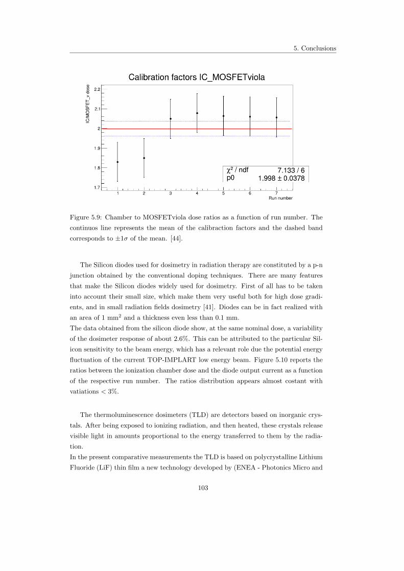
5. Conclusions
Figure 5.9: Chamber to MOSFETviola dose ratios as a function of run number. The
continuos line represents the mean of the calibraction factors and the dashed band
corresponds to ±1σ of the mean. [44].
The Silicon diodes used for dosimetry in radiation therapy are constituted by a p-n
junction obtained by the conventional doping techniques. There are many features
that make the Silicon diodes widely used for dosimetry. First of all has to be taken
into account their small size, which make them very useful both for high dose gradi-
ents, and in small radiation fields dosimetry [41]. Diodes can be in fact realized with
an area of 1 mm2 and a thickness even less than 0.1 mm.
The data obtained from the silicon diode show, at the same nominal dose, a variability
of the dosimeter response of about 2.6%. This can be attributed to the particular Sil-
icon sensitivity to the beam energy, which has a relevant role due the potential energy
fluctuation of the current TOP-IMPLART low energy beam. Figure 5.10 reports the
ratios between the ionization chamber dose and the diode output current as a function
of the respective run number. The ratios distribution appears almost costant with
vatiations < 3%.
The thermoluminescence dosimeters (TLD) are detectors based on inorganic crys-
tals. After being exposed to ionizing radiation, and then heated, these crystals release
visible light in amounts proportional to the energy transferred to them by the radia-
tion.
In the present comparative measurements the TLD is based on polycrystalline Lithium
Fluoride (LiF) thin film a new technology developed by (ENEA - Photonics Micro and
103

5. Conclusions
Figure 5.10: Chamber to Silicon diode response ratios as a function of run number.
The continuos line represents the mean of the calibraction factors and the dashed band
corresponds to ±1σ of the mean. Silicon data from [43].
Nano Structures Laboratory)[42]. The dose values, in arbitrary units, have been ob-
tained heating each exposed LiF-TLD and then detecting the thermoluminescent light
by a photomultiplier. These dose values have been compared to the ionization chamber
responses and then calibration factors have been determined. Figure 5.11 evinces the
almost costant trend of these coefficients with a confidence value CV∼ 1.4%.
The above new measurements, by different dosimeters, show a better consistency
between the different detector responses, respect to the previous measurements (re-
ported in the main text of the thesis). The ionization chamber measured doses, prelim-
inary corrected by the most relevant effects, agree within 2% to the Alanine reference
doses, as well as to the other (uncorrected) dosimeters values, within less than 3%
(once the respective calibration factors are applied).
104
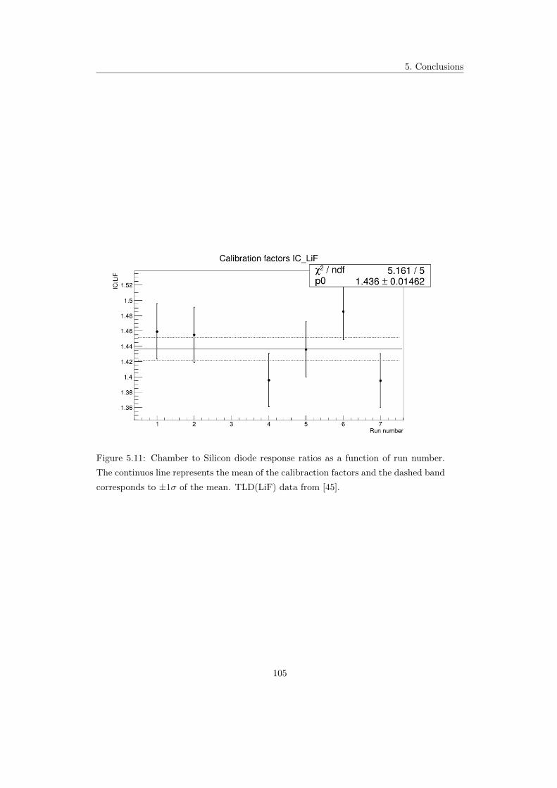
5. Conclusions
Figure 5.11: Chamber to Silicon diode response ratios as a function of run number.
The continuos line represents the mean of the calibraction factors and the dashed band
corresponds to ±1σ of the mean. TLD(LiF) data from [45].
105

Bibliography
[1] U. Amaldi, S. Braccini, Present and future of hadrontherapy, AIP Conf. Proc.
827, 248 (2006), Varenna, Italia.
[2] U. Amaldi, Cancer therapy with particle accelerators, Nuc. Phy. A654, pp. 375c-
399c, 1999.
[3] R. Wilson, Radiological use of fast protons, Radiology 47: 487-491, 1946.
[4] A. Bracco, G.-E. K orner (coordinators), Nuclear Physics for Medicine, NuPECC
Report 2013, Chapter 1, ESF.
[5] Particle Therapy Co-Operative Group web page: http://ptcog.ch/
[6] W. Wieszczycka, W Scharf, Proton Radiotherapy Accelerators, World Scientific
Publishing Co Pte Ltd, 2001.
[7] G. Knoll, Radiation Detection and Measurement, Wiley, 2010.
[8] D. Cussol, Nuclear Physics and Hadrontherapy, LPC Caen, ENSICAEN, Univer-
site de Caen Basse-Normandie, IN2P3/CNRS, 2011.
[9] U. Amaldi, Radiation Physics: Photons and Charged Hadrons, webpage
https://physique.cuso.ch/fileadmin/physique/document/Amaldi-Rad.-Trento-
2001.pdf
[10] M. Durante, H. Paganetti, Nuclear physics in particle therapy: a review, Rep.
Prog. Phys. 79 (2016).
[11] W. Newhauser, R. Zhang, The physics of proton therapy, Phys. Med. Biol 60
(2015) R155-R209.
[12] H. Paganetti, Proton therapy physics, Taylor and Francis Group, 2012.
[13] J. Rosenblatt, Particle Acceleration, Metuen, 1968.
106

BIBLIOGRAPHY
[14] S.Braccini, Medical Applications of Particle Physics, Laboratory for High Energy
Physics, University of Bern, 2008.
[15] H. Owen, D. Holder, J. Alonso, R. Mackay, Technologies for Delivery of Proton
and Ion Beams for Radiotherapy, Int. J. Mod. Phys. 2013
[16] W. Leo, Techniques for Nuclear and Particle Physics Experiments, Springer.
[17] G. Boissonnat et al, Measurement of ion and electron drift velocity and electronic
attachment in air for ionization chambers, arXiv 1609.0374v1, 2016 .
[18] L. Picardi, C. Ronsivalle, A. Vignati. Progetto del TOP Linac, ENEA - Diparti-
mento Innovazione, Centro Ricerche Frascati, Roma, 1997.
[19] C. Ronsivalle et al, The TOP-IMPLART Project, Eur. Phys. J. Plus (2011) 126:
68.
[20] P. Nenzi, A. Ampollini, G. Bazzano, L. Picardi, M. Piccinini, C. Ronsivalle, V.
Surrenti, E. Trinca, M. Vadrucci, Commissioning Results of the TOP-IMPLART
27 MeV Proton Linear Accelerator, International Beam Instrumentation Confer-
ence, IBIC 2016.
[21] U. Amaldi, A. De Giovanni, Proton and Carbon Linacs for Hadrontherapy, 27th
Linear Accelerator Conference, Geneva, Switzerland, 2014.
[22] G. Mazza et al, A 64-channel Wide Dynamic Range Charge Measurement ASIC
for strip and pixel ionization detectors, IEEE Transactions on Nuclear Science, 52
(2005) 847.
[23] IVC102, Datasheet.
[24] A. Carloni, Characterization of proton beams using Pad-Strip ionization cham-
bers fo online measurement of relative dose on phantoms in cancer therapy with
protons, tesi di laurea AA 2010/2011.
[25] E. Podgorsak, Radiation Oncology Physics, IAEA, 2015.
[26] D.M. Castelluccio, A novel realtime beam monitoring system in proton therapy
treatments, tesi di specializzazione. AA 2009/2010
[27] E. Cisbani et al., Monitor di fascio per il TOP LINAC: sviluppo dell’uso di protoni
nella terapia oncologica, Rapporti ISTISAN, Istituto Superiore di Sanita, 2004.
[28] E. Basile et al., An online proton beam monitor for cancer therapy based on ioniza-
tion chambers with micro pattern readout, 2nd International conference on Micro
Pattern Gaseous Detectors, 2011, Kobe, Japan.
107

BIBLIOGRAPHY
[29] A. Knopf, A. Lomax, In vivo proton range verification: a review, Phys. Med. Biol.
58 (2013) R131-R160.
[30] U. Amaldi, Cyclinac: fast cycling accelerators for hadrontherapy,
[31] E. Cisbani et al., Beam micro pattern ionization chamber with adaptive amplifiers
as dose delivery monitor for the therapeutic proton LINAC, International Beam
Instrumentation Conference, IBIC 2016.
[32] F. Ambrosini Ottimizzazione di una ”facility” di irraggiamento sperimentale con
protoni, Tesi di laurea magistrale, AA 2012-2013.
[33] N. Givehchi et al., Online monitor detector for the protontherapy beam at the
INFN Laboratori Nazionali del Sud-Catania, Nuclear Instruments and Methods
in Physics Research, A 572 (2007) 1094-1101.
[34] D. Lewis, A. Micke, X. Yu, An efficient protocol for radiochromic film dosimetry
combining calibratipon and measurement in a single scan, Med. Phys. 39(10),
2012.
[35] V. Nagy, S. Sholom, V. Chumak, M. Desrosiers Uncertainties in alanine dosimetry
in the therapeutic dose range, Applied Radiation and Isotopes 56 (2002) 917-929
[36] V. Casanova Borca, M. Pasquino, G. Russo, P. Grosso, D. Cante, P. Sci-
acero, G. Girelli, M. La Porta, S. Tofani Dosimetric characterization and use of
GAFCHROMIC EBT3 film for IMRT dose verification. Journal of applied clinical
medical physics, Vol 14, n 2, 2013.
[37] A. Lennox, Hospital-based proton linear accelerator for particle therapy and ra-
dioisotope production, Nuclear Instruments and Methods in Physics Research
B56/57 (1991) 1197-1200.
[38] A. Citterio, Conception and design of innovative ion linacs for hadrontherapy,
PhD Thesis, Universita di Milano, Bicocca, 2007.
[39] S. Rossi, Adroterapia: applicazione delle tecnologie degli acceleratori alla cura
dei tumori, Fondazione CNAO, Corso di Formazione Dipartimento di Fisica la
Sapienza, Roma, 2013.
[40] S. Rossi, The status of CNAO, The european physical journal plus, Springer, 2011.
[41] A. Rosenfeld, Advanced Semiconductor Dosimetry in Radiation Therapy, Univer-
sity of Wollongong Research Online, 2011. http://dx.doi.org/10.1063/1.3576159
108

BIBLIOGRAPHY
[42] M. Piccinini et al., Photoluminescence of radiation-induced color centers in lithium
fluoride thin films for advanced diagnistics of proton beams, Applied Physics Let-
ters 106, 261108 (2015).
[43] C. De Angelis, Private Communication, 2016.
[44] A. Soriani, Private Communication, 2016.
[45] M. Piccinini, Private Communication, 2016.
109