The Distribution of Wealth and the MPC:Implications of New European Data

February 11, 2014

Christopher D. Carroll1 Jiri Slacalek2 Kiichi Tokuoka3

AbstractUsing new micro data on household wealth from fifteen European countries (the House-

hold Finance and Consumption Survey), we first document substantial cross-country varia-tion in how various measures of wealth are distributed across individual households. Throughthe lens of a standard, realistically calibrated model of buffer-stock saving with transitoryand permanent income shocks we then study how cross-country differences in the wealthdistribution and household income dynamics affect the marginal propensity to consumeout of transitory shocks (MPC). We find that the aggregate consumption response rangesbetween 0.1 and 0.4 and is stronger (i) in economies with large wealth inequality, where alarger proportion of households has little wealth, (ii) under larger transitory income shocksand (iii) when we consider households only using liquid assets (rather than net wealth) tosmooth consumption.

Keywords Marginal Propensity to Consume, Wealth Distribution,Liquid Assets, Cross-Country Comparisons, HouseholdFinance and Consumption Survey

JEL codes D12, D31, D91, E21

A condensed version of this paper was published in The American Eco-nomic Review 104(5):107–111, May 2014

PDF: http://econ.jhu.edu/people/ccarroll/papers/cstMPCxc.pdfSlides: http://econ.jhu.edu/people/ccarroll/papers/cstMPCxc-Slides.pdf

Web: http://econ.jhu.edu/people/ccarroll/papers/cstMPCxc/Archive: http://econ.jhu.edu/people/ccarroll/papers/cstMPCxc.zip

1Carroll: Department of Economics, Johns Hopkins University, Baltimore, MD, http://econ.jhu.edu/people/ccarroll/,ccarroll@jhu.edu 2Slacalek: European Central Bank, Frankfurt am Main, Germany, http://www.slacalek.com/,jiri.slacalek@ecb.europa.eu 3Tokuoka: Ministry of Finance, Tokyo, Japan, kiichi.tokuoka@mof.go.jp

This paper uses data from the Eurosystem Household Finance and Consumption Survey. We thank participantsin the European Central Bank Conference on Household Finance and Consumption for helpful comments. The viewspresented in this paper are those of the authors, and should not be attributed to the European Central Bank or theJapanese Ministry of Finance.

Figure 1 The Gini Coefficients for Net Wealth0

0.2

0.4

0.6

0.8

Gin

i Coe

ffici

ents

--

Net

Wea

lth

All Cou

ntrie

s

Austri

a

Belgium

Cypru

s

Germ

any

Spain

Finlan

d

Franc

e

Greec

eIta

ly

Luxe

mbo

urg

Malt

a

Nethe

rland

s

Portu

gal

Sloven

ia

Slovak

ia

Source: The Eurosystem Household Finance and Consumption Survey.

Notes: The figure shows the Gini coefficient for net wealth, defined as the sum of real assets (including housing)and financial assets, net of total liabilities. The data cover the following countries: Austria, Belgium, Cyprus,Germany, Spain, Finland, France, Greece, Italy, Luxembourg, Malta, the Netherlands, Portugal, Slovenia and Slovakia.Reference year: mostly 2010; see Eurosystem Household Finance and Consumption Network (2013b), Table 9.1. TheGini coefficient for ‘All Countries’ was calculated by aggregating household-level data country by country usingestimation weights (which give the number of households in the population each observation represents).

1 IntroductionConsiderable evidence has recently confirmed the plausible implication of economictheory that low-wealth households should consume more out of a transitory shock toincome than high-wealth households (that is, the Marginal Propensity to Consumeis declining in wealth).1 Recent work by Carroll, Slacalek, and Tokuoka (2013b)(henceforth, CST) argues that when a standard buffer-stock model of consumptionis calibrated to match the US wealth distribution, it yields MPCs that are consistentwith the extensive empirical evidence that the MPC out of transitory shocks is very

1See Carroll, Slacalek, and Tokuoka (2013b) for an extensive literature review.

2

far from zero. (The model’s implied aggregate MPCs range from 0.2 to as high as0.6, depending on which measure of wealth is matched).This paper shows how the CST model can be adapted to the various wealth distri-

butions that have recently been measured for a set of European countries in the newlyreleased Household Finance and Consumption Survey (HFCS). The HFCS indicatesthat wealth inequality varies considerably across the fifteen European countries itcovers. (Figure 1 shows that the Gini coefficient ranges roughly between 0.45 and0.8; the latter value broadly comparable with the data for the US.2, 3)Depending on the measure of wealth that is matched (total net worth or liquid

assets), the interaction between the model’s concave consumption function and thedistribution of wealth implies aggregate MPCs ranging from 0.1 to 0.4 in the Europeancountries. The model’s prediction for MPCs in these European countries are some-what lower than the version calibrated for the US because European households tendto hold more wealth than Americans and because wealth is more equally distributedin Europe than in the US.We explore two aspects of heterogeneity: in the wealth distribution and income

uncertainty. The wealth distribution affects the MPC through level and throughinequality, as captured in the Gini coefficient. Countries in which households tendto hold less wealth respond more strongly to transitory income shocks. Similarly,countries with more pronounced wealth inequality have a higher aggregate MPC andalso a larger dispersion of MPCs across households.Household-level income dynamics affect the aggregate MPC mainly through the

size of transitory shocks, against which households can better insure themselves thanagainst permanent shocks. An increase in the variance of transitory shocks implies amore concave consumption function with a steeper slope close to the origin, and thusa higher value of the aggregate MPC.Our research builds on the work from a number of streams: (i) measurement

of the wealth distribution across countries,4 (ii) estimation of income dynamics atpersonal/household level,5 (iii) empirical work on estimating the MPC6 and (iv)calibration and solving models with heterogeneity.7The paper proceeds as follows. Section 2 lays out the theoretical model. Section 3

2The Gini coefficient for the US for 2010 of 0.87 exceeds its pre-crisis values for the 1990s and 2000s of roughly0.8.

3Of key importance for wealth inequality is the home-ownership rate; low home-ownership (in countries such asGermany and Austria) implies a high vale of the Gini coefficient (and vice versa).

4Systematic cross-country comparisons of the distribution of household wealth are infrequent; see EurosystemHousehold Finance and Consumption Network (2013a) for an overview of key stylized facts on the distribution andcomposition of wealth in our dataset.

5See, e.g., Meghir and Pistaferri (2011) for a literature review and Review of Economic Dynamics (2010) forinternational evidence; see also references in Table 1 of Carroll, Slacalek, and Tokuoka (2013a).

6See, e.g., Souleles (2002), Johnson, Parker, and Souleles (2009), Shapiro and Slemrod (2009) and other referencesin Table 1 of Carroll, Slacalek, and Tokuoka (2013b).

7See Krusell and Smith (1998) and Castaneda, Diaz-Gimenez, and Rios-Rull (2003) for seminal contributions.

3

presents key stylized facts on the wealth distribution in the new data from fifteenEuropean countries. Section 4 presents the distribution of the MPCs across countriesand households, implied by the model, and summarizes the relationships between thewealth distribution, income dynamics and the MPC. Section 5 concludes.

2 Buffer-Stock Saving Framework With a Realistic IncomeProcess and Modest Heterogeneity in Impatience

2.1 The ModelThe model follows closely Carroll, Slacalek, and Tokuoka (2013b) and consists of thefollowing components:

1. Household income process yyyt (‘Friedman/Buffer Stock’ income process, FBS)with a permanent (ψt) and a transitory (ξt) idiosyncratic shock:

yyyt = ptξtWt, (1)pt = pt−1ψt, (2)

where Wt denotes the aggregate wage rate. The transitory component is:

ξt = µ with probability u,= (1− τ)`θt with probability 1− u,

where µ > 0 is the unemployment insurance payment when unemployed, τ isthe rate of tax collected to pay unemployment benefits, ` is time worked peremployee and θt is white noise.

The motivation for this income process goes back to Friedman (1957). Vastempirical literature (see footnote 5) has since then investigated statistical prop-erties of various measures of income in numerous datasets and concluded thatthe process (1)–(2) closely resembles the data and that both the transitory andthe permanent (or highly persistent) component are important to capture actualincome dynamics.

2. The perpetual-youth mechanism of Blanchard (1985): To ensure that the ergodiccross-sectional distribution of permanent income exists, households die stochas-tically with a constant intensity D ≡ 1 −��D and are replaced with newbornsearning permanent income equal to the population mean. When the probabilityof dying is large enough, it outweighs the effect of permanent shocks and ensuresthat the ergodic distribution of income exists (and has a finite variance).8

8Carroll, Slacalek, and Tokuoka (2013a) show that the ergodic cross-sectional distribution of permanent incomeexists if �DE(ψ2) < 1.

4

3. Modest heterogeneity in impatience: While the FBS process with permanentincome shocks substantially improves the model’s fit of the empirical wealthdistribution, a bit of additional ex ante heterogeneity is necessary to ensure anadequate fit (which is important for drawing correct quantitative implicationsabout the MPC). As in the ‘β-Dist’ model of Carroll, Slacalek, and Tokuoka(2013b), we assume that households in the economy differ in time preferencefactors β, which are distributed uniformly between β̀ − ∇ and β̀ + ∇. Weestimate β̀ and ∇ by fitting the wealth Lorenz curve implied by the model tothat in the data:

{β̀,∇} = argmin{β,∇}

∑i = 20, 40, 60, 80

(wi(β,∇)− ωi

)2 (3)

subject to the constraint that the aggregate wealth-to-output ratio in the modelmatches the aggregate capital-to-output ratio from the perfect foresight model.9In the above we denote wi and ωi the proportion of total wealth held by the topi percent of households in the model and in the data, respectively.

Each household maximizes its lifetime expected discounted CRRA utility:

Et∞∑n=0

βnccc1−ρt+n

1− ρ.

The household consumption functions {ct+n}∞n=0 satisfy:

v(mt) = maxct

u(ct) + β��DEt(ψ1−ρt+1 v(mt+1)

)(4)

s.t.at = mt − ct, (5)

kt+1 = at/

(��Dψt+1), (6)mt+1 = (k + r)kt+1 + ξt+1, (7)at ≥ 0, (8)

where the variables are divided by the level of permanent income, so that the onlystate variable is (normalized) cash-on-hand mt. The three steps (5)–(7) in theevolution of household’s market resources account for the probability of dying D, thedepreciation factor for capital k = 1− δ and the interest rate r , so that the effectiveinterest rate is (k + r)/��D. The production function is Cobb–Douglas, ZKKKα(`LLL)1−α,where Z is aggregate productivity, KKK is capital, ` is time worked per employee and LLLis employment. The wage rate and the interest rate are equal to the marginal productof labor and capital, respectively.

9The capital-to-(quarterly) output ratio is set equal to 10.26 (the value used for the US by Carroll, Slacalek, andTokuoka (2013b)).

5

A target wealth-to-permanent-income ratio exists if households are impatientenough in the sense that ‘the Death-Modified Growth Impatience Condition’ ofCarroll, Slacalek, and Tokuoka (2013a) holds.10

2.2 CalibrationThe model is calibrated at the quarterly frequency following Carroll, Slacalek, andTokuoka (2013b), Table 3 and the Journal of Economic Dynamics and Control (2010)volume on comparing solution methods for the Krusell and Smith (1998) model.11The calibration and estimation of the model here differs from that in Carroll,

Slacalek, and Tokuoka (2013b) in two ways: The distribution of wealth (see section 3below) and the parametrization of the income process. The estimates of the FBSincome process for European countries, summarized in Table 1, are much scarcer thanfor the US; the key contributions are in the Review of Economic Dynamics (2010)volume on ‘Cross-Sectional Facts for Macroeconomists’ (which reports the evidencefrom Germany, Italy and Spain). The rows ‘Our Calibration’ display the values weuse.12

3 The Wealth Distribution Across and WithinCountries

We measure the wealth distribution using data from the Household Finance andConsumption Survey, a new cross-country comparable household-level dataset pro-duced by euro area central banks.13 The recently released survey provides detailedinformation on balance sheets of more than 62,000 households from fifteen euro areacountries and is thus an ideal source for cross-country comparisons of how variousmeasures and components of wealth are distributed across households.

10The condition is an amalgam of the discount factor, interest rate, the coefficient of relative risk aversion, expectedincome growth, the probability of dying and variance of permanent shocks to income; see Appendix C in Carroll,Slacalek, and Tokuoka (2013a).

11The model presented here does not include aggregate shocks; see Carroll, Slacalek, and Tokuoka (2013b), whoshow that aggregate shocks essentially do not affect the model’s quantitative implications for the MPC.

12One would hope that the institutional features of individual countries, such as the progressiveness of incometaxes and the generosity of unemployment benefits would be more clearly reflected in the estimates of variances ofshocks. Table 1 does not point to the fact that, e.g., these variance would be substantially smaller in countries suchas Germany. This may be due to measurement and sampling errors.Blundell, Graber, and Mogstad (2013) document in high-quality administrative data from Norway that the variancesof shocks to market (pretax) income clearly exceed those of disposable (after-tax) income. (The Norwegian data alsoreflect the presence transitory income shocks (as opposed to just measurement error).) See also Rostam-Afschar andYao (2013) on the effects of the tax and transfer system on precautionary saving.

13For more information on the Household Finance and Consumption Survey see the web site,http://www.ecb.europa.eu/home/html/researcher_hfcn.en.html and also Eurosystem Household Finance andConsumption Network (2013a) and Eurosystem Household Finance and Consumption Network (2013b).

6

Table 1 Estimates of the FBS Income Process in Europe

Income Process: yyyt = ptξt, pt = pt−1ψt

Variance of Income ShocksCountry/Authors Permanent• σ2

ψ Transitory σ2ξ Dataset

FranceOur Calibration 0.010 0.031Le Blanc and Georgarakos (2013)? 0.010 0.031 ECHP

GermanyOur Calibration 0.010 0.05Fuchs-Schuendeln, Krueger, and Sommer (2010)‡ 0.01–0.096 0.04–0.19 GSOEPLe Blanc and Georgarakos (2013)? 0.006 0.030 ECHPRostam-Afschar and Yao (2013) 0.030 0.054 GSOEPYao (2011)§ 0.008–0.015 0.07–0.09 GSOEP

ItalyOur Calibration 0.010 0.075Jappelli and Pistaferri (2010)‡ 0.02 0.075 SHIWLe Blanc and Georgarakos (2013)? 0.007 0.105 ECHP

SpainOur Calibration 0.010 0.05Pijoan-Mas and Sanchez-Marcos (2010)‡ 0.01–0.15 ∼ 0.03 ECPFAlbarran, Carrasco, and Martinez-Granado (2009)� 0.015–0.157 0.032–0.162 ECPF/ECHPLe Blanc and Georgarakos (2013)? 0.001 0.113 ECHP

Other European CountriesOur Calibration 0.010 0.010

Memo: United StatesCarroll, Slacalek, and Tokuoka (2013a) 0.010 0.010 Calibrated

Notes: ECHP: European Community Household Panel, GSOEP: German Socio–Economic Panel, SHIW: Survey ofHousehold Income and Wealth, ECPF: Encuesta Continua de Presupuestos Familiares; •: For this calibration ofother parameters variance of permanent shocks cannot be increased much above 0.01 for the ‘Death-Modified GrowthImpatience Condition’ described in footnote 10 to be satisfied. (Results of section 4.3 below suggest the MPCs impliedby the model are quite robust to alternative calibrations of variance of income shocks.) ?: See Table 5 in Le Blancand Georgarakos (2013), ‡: See Table 7A–C in Review of Economic Dynamics (2010), pages 11–13, �: See Figures 3and 4 in Albarran, Carrasco, and Martinez-Granado (2009), page 509. §: Implied by Table 1 in Yao (2011).

7

Figure 2 displays the distribution of wealth-to-permanent income ratios (see alsoTable 6 in the Appendix). Net wealth is defined as the sum of value of real and finan-cial assets, net of total liabilities. Liquid financial and retirement assets are definedas the sum of value of deposits, mutual funds, non-self-employment business wealth,shares, managed accounts and voluntary private pensions/whole life insurance. Weapproximate permanent income by restricting the sample to households which in thesurvey respond that their current income equals roughly to their ‘normal’ income.Several facts are relevant for our results below. First, substantial heterogeneity in

ratios both across and within countries—up to the multiple of 100 or so of quarterlyincome—suggests that the MPCs will vary across individual households (because ofconcavity of the consumption function) and they will imply different reactions ofaggregate consumption across countries.

Figure 2 The Distribution of Wealth-to-Income Ratios Across and WithinCountries

050

100

150

Wea

lth-I

ncom

e R

atio

s (Q

uart

erly

)

Austri

a

Belgium

Cypru

s

Germ

any

Spain

Finlan

d

Franc

e

Greec

eIta

ly

Luxe

mbo

urg

Malt

a

Nethe

rland

s

Portu

gal

Sloven

ia

Slovak

ia

excludes outside values

Net Wealth Liquid Assets

Source: The Eurosystem Household Finance and Consumption Survey.

Notes: The figure shows a box plot with the lower adjacent value, the 25th percentile, the median, the 75th percentileand the upper adjacent value. The adjacent values are the 25th percentile − 1.5×interquartile range and the 75thpercentile + 1.5×interquartile range. The figure shows only the results for households which state that their currentincome equals roughly to their ‘normal’ income (variable HG0700 in the survey). The sample is restricted to householdswith non-negative holdings of net wealth/liquid assets and with the reference person aged 25–60 years.

8

Second, across all countries, the distribution of liquid assets lies substantially closerto zero than the distribution of net wealth, which points toward the hypothesis thata model calibrated to the distribution of liquid assets will imply higher MPCs than amodel calibrated to the distribution of net wealth.Third, the dispersion of the distribution of liquid assets, as reflected, e.g., in

the rectangles in Figure 2 showing the interquartile range, is considerably morecompressed.

4 Marginal Propensity, Wealth Distribution andIncome Dynamics

We will now use our model economies to back out quantitatively how the distributionof wealth affects the distribution of the MPC and the reaction of aggregate spendingto shocks, such as a ‘fiscal stimulus.’

4.1 The Role of the Wealth DistributionTo apply the model of section 2, we alternatively target two wealth variables: netwealth, and liquid financial and retirement assets. These two wealth targets illustratea range of resources that households can use to smooth adverse shocks.As argued by Otsuka (2003), Kaplan and Violante (2011) and others, a key factor

determining the response of consumer spending is liquidity of assets held by house-holds, i.e., the cost households have to incur if they use their assets to smoothconsumption. The model estimated for the distribution of net wealth implicitlyassumes that all assets (including housing) are completely liquid, while the modelestimated for liquid assets assumes that housing assets are completely illiquid andare not used to smooth consumption. A realistic case in which different assets canbe rebalanced at different costs (also depending on, e.g., availability and cost ofmortgage equity withdrawal across countries) thus likely lies between these two polarcases reported in Tables 3 and 4.To summarize the tables, the model of section 2 implies the following facts:

1. As also shown in Figure 3, aggregate MPCs range between 0.1 and 0.2 whenfitting the distribution of net wealth and roughly between 0.2 and 0.4 whenfitting the distribution of liquid assets.14

These estimates are in the lower range of values from numerous empiricalstudies, which typically find an MPC between 0.2 and 0.6 (investigating mostlyvarious fiscal stimulus episodes in the US).15 Our model thus implies sharply

14We discuss possible determinants of the cross-country variation in MPC below.15Our model fitted to the US wealth distribution implies an aggregate MPC of around 0.2–0.6.

9

Tab

le2

Distributionof

Wealth-to-Perman

entIncomeRatios

Statistic

All

Austria

Cyp

rus

Spain

Fran

ceItaly

Malta

Portuga

lSlovak

iaCou

ntries

Belgium

German

yFinland

Greece

Luxm

brg

Nethrlds

Sloven

ia

Net

Wealth

10%

1.6

1.5

2.2

6.0

1.2

4.2

1.4

1.5

2.1

2.3

2.2

9.9

1.8

1.8

3.8

6.9

25%

4.2

2.9

6.6

13.9

2.7

13.7

2.9

3.0

7.4

5.6

6.3

19.6

4.1

6.2

10.2

12.1

50%

13.

89.6

15.6

27.7

7.6

26.9

9.0

12.6

16.9

19.7

17.4

30.5

10.8

16.8

20.4

19.6

75%

27.

825.1

29.0

52.3

16.9

43.3

17.9

26.5

30.6

34.3

29.9

58.2

20.7

32.9

35.3

31.7

Mean

21.

120.0

23.7

40.8

13.3

33.7

13.6

20.0

23.9

25.1

24.0

43.0

16.5

25.5

29.5

25.9

Fraction

ofHou

seho

ldswith

WY<

2?

0.14

0.1

60.

090.

040.

200.

050.

170.

170.

090.

080.

090.

010.

120.

110.

050.

02GiniC

oefficient�

0.69

0.7

70.

61

0.69

0.78

0.58

0.70

0.68

0.56

0.61

0.69

0.61

0.69

0.64

0.55

0.45

Liqu

idFinan

cial

andRetirem

entAssets

10%

1.1

1.1

1.1

1.0

1.1

1.1

1.0

1.1

1.0

1.0

1.1

1.4

1.1

1.0

1.0

1.1

25%

1.3

1.5

1.6

1.6

1.3

1.4

1.2

1.3

1.0

1.4

1.5

2.4

1.5

1.2

1.1

1.3

50%

2.2

2.5

3.5

3.2

2.6

2.1

1.7

2.1

1.4

2.2

2.5

4.7

3.6

1.8

1.5

2.0

75%

4.5

4.9

7.0

6.8

5.2

4.1

2.9

4.1

2.4

3.8

4.6

9.4

8.6

3.9

2.8

3.4

Mean

4.3

4.8

7.7

6.8

4.2

4.4

2.9

3.9

2.6

3.3

4.5

7.3

7.3

4.1

2.9

3.3

Fraction

ofHou

seho

ldswith

LQA–Y<

2?0.

450.4

00.

290.

330.

410.

470.

600.

490.

670.

450.

380.

200.

340.

550.

670.

50GiniC

oefficient�

0.75

0.7

30.

76

0.74

0.70

0.80

0.77

0.77

0.81

0.73

0.71

0.59

0.60

0.78

0.77

0.70

Source:The

Eurosystem

Hou

seho

ldFinan

cean

dCon

sumptionSu

rvey.

Notes:Ratiosto

quarterlyho

useholdincome.

The

tabledisplays

only

thestatistics

forho

useholds

which

statethat

theircurrentincomeequa

lsroug

hlyto

their

‘normal’income(variableHG0700

inthesurvey).

The

sampleis

restricted

toho

useholds

withno

n-negative

holdings

ofnetwealth/

liquidassets

andwiththe

referencepe

rson

aged

25–60years.?:Fraction

ofho

useholds

withwealth–

quarterlyincomeratiobe

low

2.�:Calculatedforlevelo

fnetwealth/

liquidassets

(not

wealth–

incomeratio).

10

Figure 3 Aggregate MPC: Range Implied by Matching the Distribution of NetWealth and of Liquid Assets

00.

10.

20.

30.

40.

5A

ggre

gate

MP

C

All Cou

ntrie

s

Austri

a

Belgium

Cypru

s

Germ

any

Spain

Finlan

d

Franc

e

Greec

eIta

ly

Luxe

mbo

urg

Malt

a

The N

ethe

rland

s

Portu

gal

Sloven

ia

Slovak

ia

Notes: The figure shows the range of aggregate MPCs spanned by the estimates based on the distribution of netwealth (lower bound, Table 3) and of liquid assets (upper bound, Table 4).

11

Tab

le3

The

Margina

lPrope

nsity

toCon

sume,

MatchingtheDistributionof

Net

Wealth

All

Austria

Cyp

rus

Spain

Fran

ceItaly

Malta

Portuga

lSlovak

iaCou

ntries

Belgium

German

yFinland

Greece

Luxm

brg

Nethrlds

Sloven

ia

Overall

Average

0.12

0.16

0.10

0.13

0.22

0.12

0.13

0.13

0.10

0.13

0.12

0.10

0.11

0.11

0.10

0.10

Bywealth-to-perman

entincomeratio

Top

1%0.06

0.06

0.06

0.06

0.05

0.06

0.06

0.06

0.06

0.06

0.06

0.06

0.06

0.06

0.06

0.06

Top

10%

0.06

0.06

0.06

0.06

0.06

0.06

0.06

0.06

0.06

0.06

0.06

0.06

0.06

0.06

0.06

0.06

Top

20%

0.06

0.06

0.06

0.06

0.06

0.06

0.06

0.06

0.06

0.06

0.06

0.06

0.06

0.06

0.06

0.06

Top

40%

0.06

0.06

0.06

0.06

0.07

0.06

0.06

0.06

0.06

0.07

0.06

0.06

0.06

0.06

0.06

0.06

Top

50%

0.06

0.07

0.06

0.06

0.08

0.07

0.06

0.07

0.06

0.07

0.06

0.06

0.06

0.06

0.06

0.07

Top

60%

0.07

0.07

0.07

0.07

0.09

0.07

0.07

0.07

0.06

0.07

0.07

0.07

0.07

0.07

0.06

0.07

Bottm

50%

0.17

0.25

0.14

0.19

0.34

0.17

0.19

0.19

0.13

0.19

0.17

0.14

0.16

0.15

0.13

0.13

Byincome

Top

1%0.09

0.13

0.07

0.09

0.15

0.07

0.09

0.09

0.07

0.08

0.09

0.07

0.08

0.08

0.07

0.07

Top

10%

0.09

0.13

0.07

0.10

0.16

0.08

0.10

0.10

0.07

0.09

0.09

0.07

0.08

0.08

0.07

0.07

Top

20%

0.10

0.14

0.08

0.11

0.16

0.09

0.11

0.10

0.08

0.09

0.10

0.08

0.09

0.09

0.08

0.08

Top

40%

0.11

0.15

0.10

0.12

0.18

0.10

0.12

0.12

0.09

0.11

0.11

0.10

0.11

0.10

0.09

0.09

Top

50%

0.12

0.16

0.10

0.13

0.19

0.10

0.13

0.12

0.10

0.11

0.12

0.10

0.11

0.11

0.10

0.09

Top

60%

0.12

0.16

0.11

0.13

0.19

0.11

0.13

0.13

0.10

0.12

0.12

0.11

0.12

0.11

0.10

0.10

Bottm

50%

0.12

0.17

0.10

0.13

0.24

0.13

0.13

0.14

0.10

0.15

0.12

0.10

0.11

0.11

0.10

0.10

Byem

ploy

mentstatus

Employed

0.11

0.15

0.10

0.12

0.20

0.11

0.12

0.12

0.09

0.13

0.11

0.10

0.10

0.10

0.09

0.09

Unempl

0.23

0.33

0.20

0.25

0.38

0.20

0.25

0.24

0.19

0.22

0.23

0.20

0.22

0.21

0.19

0.18

Tim

epreference

parameters‡

β̀0.98

90.98

80.99

00.98

90.98

70.99

00.98

90.98

90.99

00.98

90.98

90.99

00.99

00.99

00.99

00.99

0∇

0.00

30.00

50.00

20.00

30.00

70.00

20.00

30.00

30.00

10.00

20.00

30.00

20.00

20.00

20.00

10.00

0

Notes:Average

(aggregate)prop

ensities

inan

nual

term

s.Ann

ualM

PC

iscalculated

by1−

(1−qu

arterlyMPC

)4.‡ :

Discoun

tfactorsareun

iform

lydistribu

ted

over

theinterval

[β̀−∇,β̀

+∇

].

12

Tab

le4

The

Margina

lPrope

nsity

toCon

sume,

MatchingtheDistributionof

Liqu

idFinan

cial

andRetirem

entAssets

All

Austria

Cyp

rus

Spain

Fran

ceItaly

Malta

Portuga

lSlovak

iaCou

ntries

Belgium

German

yFinland

Greece

Luxm

brg

Nethrlds

Sloven

ia

Overall

Average

0.26

0.24

0.27

0.25

0.26

0.38

0.28

0.30

0.35

0.31

0.23

0.18

0.19

0.32

0.29

0.23

Bywealth-to-perman

entincomeratio

Top

1%0.12

0.12

0.12

0.12

0.12

0.12

0.12

0.12

0.12

0.12

0.12

0.13

0.13

0.12

0.12

0.12

Top

10%

0.13

0.13

0.12

0.13

0.13

0.12

0.12

0.12

0.12

0.13

0.13

0.13

0.13

0.12

0.12

0.13

Top

20%

0.13

0.13

0.13

0.13

0.13

0.13

0.13

0.13

0.13

0.13

0.13

0.13

0.13

0.13

0.13

0.13

Top

40%

0.13

0.13

0.13

0.13

0.14

0.16

0.14

0.14

0.15

0.15

0.13

0.13

0.13

0.14

0.14

0.13

Top

50%

0.14

0.14

0.14

0.14

0.14

0.18

0.15

0.15

0.17

0.16

0.14

0.13

0.13

0.16

0.15

0.14

Top

60%

0.15

0.15

0.15

0.15

0.15

0.21

0.16

0.17

0.19

0.17

0.14

0.13

0.14

0.18

0.17

0.14

Bottm

50%

0.36

0.33

0.38

0.35

0.36

0.54

0.40

0.43

0.50

0.44

0.32

0.23

0.24

0.45

0.42

0.31

Byincome

Top

1%0.22

0.20

0.22

0.21

0.20

0.29

0.24

0.24

0.30

0.23

0.19

0.15

0.15

0.27

0.25

0.19

Top

10%

0.22

0.20

0.23

0.21

0.20

0.29

0.24

0.24

0.30

0.23

0.20

0.15

0.15

0.27

0.25

0.19

Top

20%

0.23

0.21

0.24

0.22

0.21

0.30

0.25

0.25

0.30

0.24

0.21

0.16

0.17

0.28

0.26

0.20

Top

40%

0.24

0.23

0.25

0.24

0.23

0.32

0.27

0.27

0.32

0.26

0.22

0.18

0.18

0.29

0.27

0.22

Top

50%

0.25

0.24

0.26

0.24

0.24

0.33

0.27

0.28

0.32

0.27

0.23

0.18

0.19

0.30

0.28

0.22

Top

60%

0.25

0.24

0.26

0.25

0.24

0.34

0.28

0.28

0.33

0.28

0.23

0.19

0.19

0.30

0.28

0.23

Bottm

50%

0.27

0.25

0.28

0.26

0.29

0.42

0.30

0.33

0.37

0.35

0.24

0.18

0.19

0.33

0.31

0.23

Byem

ploy

mentstatus

Employed

0.24

0.23

0.25

0.23

0.25

0.36

0.26

0.28

0.32

0.30

0.22

0.17

0.18

0.29

0.27

0.21

Unempl

0.45

0.42

0.47

0.44

0.41

0.60

0.50

0.51

0.62

0.47

0.40

0.29

0.30

0.57

0.52

0.39

Tim

epreference

parameters‡

β̀0.96

90.97

00.96

90.96

90.96

90.96

40.96

90.96

80.96

60.96

70.97

00.97

10.97

10.96

80.96

80.97

0∇

0.00

60.00

50.00

60.00

60.00

60.01

20.00

70.00

80.01

00.00

90.00

50.00

20.00

20.00

80.00

70.00

5

Notes:Average

(aggregate)prop

ensities

inan

nual

term

s.Ann

ualM

PC

iscalculated

by1−

(1−qu

arterlyMPC

)4.‡ :

Discoun

tfactorsareun

iform

lydistribu

ted

over

theinterval

[β̀−∇,β̀

+∇

].

13

different conclusions than many other models (including Krusell and Smith(1998)) in which the economy behaves in a certainty-equivalent manner andhas aggregate MPCs out of transitory income shocks of 0.02–0.05.

2. The variation in MPCs across individual households generated by concavity ofthe consumption function is substantial and economically relevant. Spending ofunemployed individuals and households earning low income and holding littlewealth is more sensitive to shocks. This fact implies that a fiscal stimulustargeted to these households has particularly large effects.

This finding is again broadly in line with a number of empirical studies, suchas Blundell, Pistaferri, and Preston (2008), Broda and Parker (2012), Kreiner,Lassen, and Leth-Petersen (2012) and Jappelli and Pistaferri (2013).

3. The estimates of the discount factor β lie around 0.99 for net wealth and 0.97for liquid assets. The extent of heterogeneity in β is very modest: ∇ ≈ 0.003and ∇ ≈ 0.006 for net wealth and liquid assets, respectively. These valuesare roughly half the size of those reported in Carroll, Slacalek, and Tokuoka(2013b) for the US (∇ ≈ 0.006–0.013), reflecting the lower wealth inequality inEuropean countries.

4. Figure 4 illustrates how the model fits the upper tail of the wealth distribution.The figure shows the ratio of the share of wealth held by the top 10 percent ofhouseholds living in the model to those living in the real world.16 The ratiostypically lie close to 1, suggesting the model performs quite well, although itoverfits the upper tail of liquid assets in a few countries.17

4.2 Wealth Inequality and Aggregate MPC: Cross-Country ResultsAn important advantage of datasets with a large country dimension, such as theHousehold Finance and Consumption Survey, is that they make it possible to compareeconomic behavior of households across countries. This section investigates howdifferences in wealth distributions across countries affect the response of economiesto shocks.18Figure 5 summarizes the relationship between wealth inequality (as measured with

the Gini coefficient) and aggregate MPCs (reported in row 1 of Tables 3 and 4). For

16Note that the top 10 percent share is not targeted in the estimation of β̀ and ∇ in equation (3) above, so thatthe statistics in Figure 4 have a bit of an ‘out-of-sample’ flavor.

17Note that for our purpose of backing out the aggregate MPC it is not vital to match the upper tail of the wealthdistribution perfectly, as the consumption function is approximately linear at the higher levels of wealth, above themedian or so.

18While we assume the wealth distribution is exogenous, in reality, it depends on institutions and policies. Forexample, as mentioned in footnote 3, an important factor for wealth inequality is the home-ownership rate, whichfurther depends on institutions, such as the size of downpayment ratios, see Chiuri and Jappelli (2003).

14

Figure 4 Fit of the Models: Ratio of the Share of Top 10 Percent of HouseholdsImplied by the Model and in the Data

00.

51

1.5

2T

op 1

0 P

erce

nt S

hare

s: M

odel

/Dat

a

All Cou

ntrie

s

Austri

a

Belgium

Cypru

s

Germ

any

Spain

Finlan

d

Franc

e

Greec

eIta

ly

Luxe

mbo

urg

Malt

a

Nethe

rland

s

Portu

gal

Sloven

ia

Slovak

ia

Net Wealth Liquid Assets

Source: The Eurosystem Household Finance and Consumption Survey and authors’ calculations.

Notes: The figure shows the ratio of the shares implied by the models to those in the data; the values close to oneindicate a good fit.

15

Figure 5 How Wealth Inequality Affects Aggregate MPC: The Gini Coefficientsand the Aggregate MPC

ALL

AT

BE

CY

DE

ESFIFR

GR

ITLU

MTNLPT

SISK

ALL

AT

BECYDE

ES

FI

FR

GR

IT

LU

MTNL

PT

SI

SK

00.

10.

20.

30.

40.

5A

ggre

gate

MP

C

0.4 0.5 0.6 0.7 0.8Gini Coefficient

Net Wealth Liquid Assets

Source: The Eurosystem Household Finance and Consumption Survey and authors’ calculations.

16

Figure 6 How Wealth Inequality Affects Inequality in MPC

ALL

AT

BE

CY

DE

ES

FI

FR

GR

ITLU

MT

NL

PT

SI

SK

ALL

AT

BE

CYDE

ES

FI

FR GR

IT

LU

MTNL

PTSI

SK

23

4M

PC

of B

otto

m 5

0% /

MP

C o

f Top

50%

, by

Wea

lth

0.4 0.5 0.6 0.7 0.8Gini Coefficient

Net Wealth Liquid Assets

Source: The Eurosystem Household Finance and Consumption Survey and authors’ calculations.

Notes: The figure shows the Gini coefficient for wealth against the ratio of the MPC for bottom and top 50 percentof households by wealth-to-permanent income ratio.

both measures of wealth, countries with more unequal wealth distributions tend tohave a higher proportion of households with little wealth and tend to respond morestrongly to shocks.19 The relationship is tighter for liquid assets as these holdings arelower than holdings of net wealth and the consumption function is more concave (andsteeper) close to the origin.Figure 6 displays the relationship between wealth inequality and heterogeneity

across MPCs (as captured in the ratio of average MPCs of the top and bottom half ofhouseholds by wealth). For both measures of wealth, the figure documents that wealthinequality affects not only the level of aggregate MPC but also the dispersion of MPCsacross individual households in the economy. Given the shape of the consumptionfunction, more pronounced wealth inequality increases the proportion of households

19Table 2 above documents a strong relationship between the Gini coefficient and the proportion of householdswith wealth-to-permanent income ratio below 2.

17

with little wealth and the MPC among the lower half of the population, while it doesnot affect the MPC of the upper half, as the consumption function is essentially linearin that region. The relationship is again tighter for liquid assets.

4.3 The Role of Income ShocksTable 1 above summarized empirical estimates of the FBS income process (1)–(2).Although in principle variance of income shocks should be related to institutionalfeatures at the country level, such as progressivity of the tax system and generosityof social benefits, empirical estimates do not seem to reflect this clearly enough.For that reason, Table 5 presents a comparative statics exercise about the role of the

size of income shocks, comparing the baseline calibration of Table 3 (for ‘all countries’)to three alternatives which differ in the variance of permanent and transitory shocks.20While the size of permanent income shocks affects the shape of the consumption

function only negligibly, empirically plausible variation in the variance of transitoryshocks generates quite substantial changes in the MPC for the whole economy and,in particular, for households with little wealth. Larger transitory shocks make theconsumption function steeper close to the origin. Specifically, an increase in σ2

θ from0.01 to 0.1 raises the average MPC from 0.13 to 0.17 for the whole population andfrom 0.19 to 0.26 for the lower 50 percent of households by wealth.

5 ConclusionsOur results document the importance of matching stylized facts at the household levelfor thinking about the reaction of economies to shocks. The precautionary savingmotive generates a concave consumption function, which means that the reaction ofspending of individual households depends on the level of wealth they hold. Dueto this substantial non-linearity, to draw correct quantitative conclusions about theaggregate behavior of the economy, it is important that the model fits the empiricalwealth distribution. Using data from fifteen European countries, we find that wealthinequality and differences in the dynamics of household income affect the response ofeconomies to a ‘fiscal stimulus’ in an economically relevant way.

20Note that the variance of permanent shocks σ2ψ cannot be increased if, for the calibration with liquid assets, all

households are to meet the condition of footnote 8, which ensures that the ergodic distribution of income exists.

18

Table 5 The MPC Under Alternative Variances of Income Shocks

Scenario Baseline Low σ2ψ High σ2

θ Very High σ2θ

σ2ψ = 0.01 σ2

ψ = 0.005 σ2ψ = 0.01 σ2

ψ = 0.01σ2θ = 0.01 σ2

θ = 0.01 σ2θ = 0.05 σ2

θ = 0.10

OverallAverage 0.12 0.12 0.14 0.17By wealth-to-permanent income ratio

Top 1% 0.06 0.06 0.06 0.06Top 10% 0.06 0.06 0.06 0.06Top 20% 0.06 0.06 0.06 0.06Top 40% 0.06 0.06 0.06 0.07Top 50% 0.07 0.07 0.05 0.07Top 60% 0.07 0.06 0.07 0.08Bottom 50% 0.17 0.17 0.22 0.26

By incomeTop 1% 0.09 0.08 0.10 0.11Top 10% 0.09 0.09 0.10 0.12Top 20% 0.10 0.10 0.11 0.12Top 40% 0.11 0.11 0.12 0.14Top 50% 0.12 0.11 0.12 0.14Top 60% 0.12 0.11 0.13 0.15Bottom 50% 0.12 0.13 0.16 0.20

By employment statusEmployed 0.11 0.11 0.14 0.16Unemployed 0.23 0.24 0.25 0.27

Time preference parameters‡

β̀ 0.989 0.990 0.989 0.988∇ 0.003 0.002 0.004 0.005

Notes: Average (aggregate) propensities in annual terms. Annual MPC is calculated by 1− (1− quarterly MPC)4. ‡:Discount factors are uniformly distributed over the interval [β̀ − ∇, β̀ +∇]. The targeted wealth distribution is thedistribution of net wealth for the full sample covering all fifteen countries.

19

ReferencesAlbarran, Pedro, Raquel Carrasco, and Maite Martinez-Granado (2009):

“Inequality for Wage Earners and Self-Employed: Evidence from Panel Data,” OxfordBulletin of Economics and Statistics, 71(4), 491–518.

Blanchard, Olivier J. (1985): “Debt, Deficits, and Finite Horizons,” Journal of PoliticalEconomy, 93(2), 223–247.

Le Blanc, Julia, and Dimitris Georgarakos (2013): “How Risky Is Their Income?Labor Income Processes in Europe,” mimeo, Goethe University Frankfurt.

Blundell, Richard, Michael Graber, and Magne Mogstad (2013): “Labor IncomeDynamics and the Insurance from Taxes, Transfers, and the Family,” mimeo, UniversityCollege London.

Blundell, Richard, Luigi Pistaferri, and Ian Preston (2008): “ConsumptionInequality and Partial Insurance,” American Economic Review, 98(5), 1887–1921.

Broda, Christian, and Jonathan A. Parker (2012): “The Economic StimulusPayments of 2008 and the Aggregate Demand for Consumption,” mimeo, NorthwesternUniversity.

Carroll, Christopher D., Jiri Slacalek, and Kiichi Tokuoka (2013a): “Buffer-Stock Saving in a Krusell–Smith World,” mimeo, Johns Hopkins University.

(2013b): “The Distribution of Wealth and the MarginalPropensity to Consume,” mimeo, Johns Hopkins University, Athttp://econ.jhu.edu/people/ccarroll/papers/cstMPC/.

Castaneda, Ana, Javier Diaz-Gimenez, and Jose-Victor Rios-Rull (2003):“Accounting for the U.S. Earnings and Wealth Inequality,” Journal of Political Economy,111(4), 818–857.

Chiuri, Maria Concetta, and Tullio Jappelli (2003): “Financial MarketImperfections and Home Ownership: A Comparative Study,” European Economic Review,47(5), 857–875.

Eurosystem Household Finance and Consumption Network(2013a): “The Eurosystem Household Finance and Consumption Survey– First Results,” Statistics Paper Series 2, European Central Bank,http://www.ecb.europa.eu/pub/pdf/other/ecbsp2en.pdf.

(2013b): “The Eurosystem Household Finance and Consumption Survey– Methodological Report,” Statistics Paper Series 1, European Central Bank,http://www.ecb.europa.eu/pub/pdf/other/ecbsp1en.pdf.

20

Friedman, Milton A. (1957): A Theory of the Consumption Function. PrincetonUniversity Press.

Fuchs-Schuendeln, Nicola, Dirk Krueger, and Mathias Sommer (2010):“Inequality Trends for Germany in the Last Two Decades: A Tale of Two Countries,”Review of Economic Dynamics, 13(1), 103–132.

Jappelli, Tullio, and Luigi Pistaferri (2010): “Does Consumption Inequality TrackIncome Inequality in Italy?,” Review of Economic Dynamics, 13(1), 133–153.

(2013): “Fiscal Policy and MPC Heterogeneity,” discussion paper 9333, CEPR.

Johnson, David S., Jonathan A. Parker, and Nicholas S. Souleles (2009): “TheResponse of Consumer Spending to Rebates During an Expansion: Evidence from the2003 Child Tax Credit,” working paper, The Wharton School.

Journal of Economic Dynamics and Control (2010): “Computational Suite ofModels with Heterogeneous Agents: Incomplete Markets and Aggregate Uncertainty,”edited by Wouter J. Den Haan, Kenneth L. Judd, Michel Juillard, 34(1), 1–100.

Kaplan, Greg, and Giovanni L. Violante (2011): “A Model of the ConsumptionResponse to Fiscal Stimulus Payments,” NBER Working Paper Number W17338.

Kreiner, Claus Thustrup, David Dreyer Lassen, and Søren Leth-Petersen(2012): “Heterogeneous Responses and Aggregate Impact of the 2001 Income TaxRebates,” discussion paper 9161, CEPR.

Krusell, Per, and Anthony A. Smith (1998): “Income and Wealth Heterogeneity inthe Macroeconomy,” Journal of Political Economy, 106(5), 867–896.

Meghir, Costas, and Luigi Pistaferri (2011): “Earnings, Consumption and Life CycleChoices,” in Handbook of Labor Economics, ed. by O. Ashenfelter, and D. Card, vol. 4,chap. 9, pp. 773–854. Elsevier.

Otsuka, Misuzu (2003): “Household Portfolio Choice with Illiquid Assets,” manuscript,Johns Hopkins University.

Pijoan-Mas, Josep, and Virginia Sanchez-Marcos (2010): “Spain Is Different:Falling Trends of Inequality,” Review of Economic Dynamics, 13(1), 154–178.

Review of Economic Dynamics (2010): “Special Issue: Cross-Sectional Facts forMacroeconomists,” 13(1), 1–264, edited by by Dirk Krueger, Fabrizio Perri, LuigiPistaferri and Giovanni L. Violante.

Rostam-Afschar, Davud, and Jiaxiong Yao (2013): “Taxation and PrecautionarySavings over the Life Cycle,” mimeo, Johns Hopkins University.

21

Shapiro, Matthew W., and Joel B. Slemrod (2009): “Did the 2008 TaxRebates Stimulate Spending?,” American Economic Review, 99(2), 374–379, http://www-personal.umich.edu/~shapiro/papers/Rebate2008-2008-12-27-assa-draft.pdf.

Souleles, Nicholas S. (2002): “Consumer Response to the Reagan Tax Cuts,” Journalof Public Economics, 85, 99–120.

Yao, Yao (2011): “Labor Income Risks in Germany,” mimeo, University of Mannheim.

Appendix: Additional Statistics on the Wealth Distribution

Table 6 displays statistics about the distribution of net wealth, and liquid financialand retirement assets across countries. The last row shows the number of observationsin the sample (which is restricted to households with the reference person aged 25–60years).

22

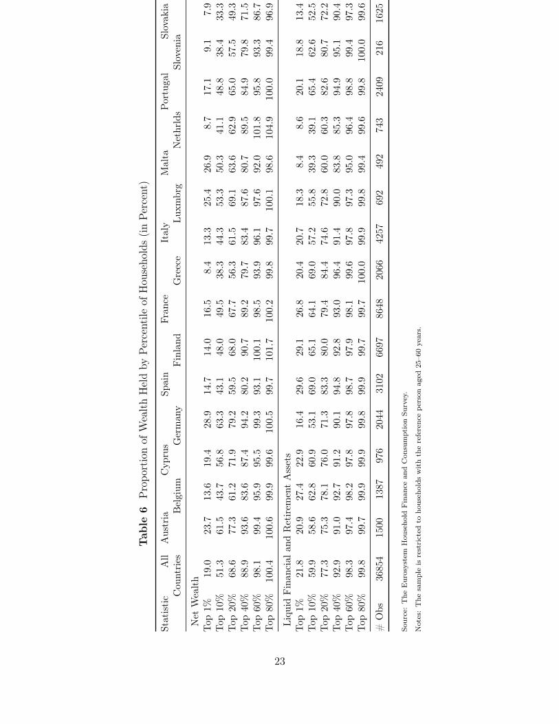
Tab

le6

Propo

rtionof

WealthHeldby

Percentile

ofHou

seho

lds(inPercent)

Statistic

All

Austria

Cyp

rus

Spain

Fran

ceItaly

Malta

Portuga

lSlovak

iaCou

ntries

Belgium

German

yFinland

Greece

Luxm

brg

Nethrlds

Sloven

ia

Net

Wealth

Top

1%19.

023.7

13.6

19.

428.9

14.7

14.0

16.5

8.4

13.3

25.4

26.9

8.7

17.1

9.1

7.9

Top

10%

51.

361.5

43.7

56.

863.3

43.1

48.0

49.5

38.3

44.3

53.3

50.3

41.1

48.8

38.4

33.3

Top

20%

68.

677.3

61.2

71.

979.2

59.5

68.0

67.7

56.3

61.5

69.1

63.6

62.9

65.0

57.5

49.3

Top

40%

88.

993.6

83.6

87.

494.2

80.2

90.7

89.2

79.7

83.4

87.6

80.7

89.5

84.9

79.8

71.5

Top

60%

98.

199.4

95.9

95.

599.3

93.1

100.

198.5

93.9

96.1

97.6

92.0

101.

895.8

93.3

86.7

Top

80%

100.

410

0.6

99.9

99.

610

0.5

99.7

101.

710

0.2

99.8

99.7

100.

198.6

104.

910

0.0

99.4

96.9

Liqu

idFinan

cial

andRetirem

entAssets

Top

1%21.

820.9

27.4

22.

916.4

29.6

29.1

26.8

20.4

20.7

18.3

8.4

8.6

20.1

18.8

13.4

Top

10%

59.

958.6

62.8

60.

953.1

69.0

65.1

64.1

69.0

57.2

55.8

39.3

39.1

65.4

62.6

52.5

Top

20%

77.

375.3

78.1

76.

071.3

83.3

80.0

79.4

84.4

74.6

72.8

60.0

60.3

82.6

80.7

72.2

Top

40%

92.

991.0

92.7

91.

290.1

94.8

92.8

93.0

96.4

91.4

90.0

83.8

85.3

94.9

95.1

90.4

Top

60%

98.

397.4

98.2

97.

897.8

98.7

97.9

98.1

99.6

97.8

97.3

95.0

96.4

98.8

99.4

97.3

Top

80%

99.

899.7

99.9

99.

999.8

99.9

99.7

99.7

100.

099.9

99.8

99.4

99.6

99.8

100.

099.6

#Obs

3685

415

0013

8797

620

4431

026697

8648

2066

4257

692

492

743

2409

216

1625

Source:The

Eurosystem

Hou

seho

ldFinan

cean

dCon

sumptionSu

rvey.

Notes:The

sampleis

restricted

toho

useholds

withthereferencepe

rson

aged

25–60years.

23