The distribution of wealth and �scal policy ineconomies with �nitely lived agents�

Jess BenhabibNYU and NBER

Alberto BisinNYU and NBER

Shenghao ZhuNUS

This draft: June 2010

Abstract

We study the dynamics of the distribution of wealth in an overlapping gen-eration economy with �nitely lived agents and inter-generational transmission ofwealth. Financial markets are incomplete, exposing agents to both labor and cap-ital income risk. We show that the stationary wealth distribution is a Paretodistribution in the right tail and that it is capital income risk, rather than laborincome, that drives the properties of the right tail of the wealth distribution. Wealso study analytically the dependence of the distribution of wealth, of wealthinequality in particular, on various �scal policy instruments like capital incometaxes and estate taxes, and on di¤erent degrees of social mobility. We show thatcapital income and estate taxes can signi�cantly reduce wealth inequality, as doinstitutions favoring social mobility. Finally, we calibrate the economy to matchthe Lorenz curve of the wealth distribution of the U.S. economy.

�We gratefully acknowledge Daron Acemoglu�s extensive comments on an earlier paper on the samesubject, which have lead us to the formulation in this paper. We also acknowledge the ideas and sugges-tions of Xavier Gabaix and �ve referees that we incorporated into the paper, as well as the conversationswith Marco Bassetto, Gerard Ben Arous, Alberto Bressan, Bei Cao, In-Koo Cho, Gianluca Clementi, Is-abel Correia, Mariacristina De Nardi, Raquel Fernandez, Leslie Greengard, Frank Hoppensteadt, BoyanJovanovic, Stefan Krasa, Nobu Kiyotaki, Guy Laroque, John Leahy, Omar Licandro, Andrea Moro, JunNie, Chris Phelan, Alexander Roitershtein, Hamid Sabourian, Benoite de Saporta, Tom Sargent, EnnioStacchetti, Pedro Teles,Viktor Tsyrennikov, Gianluca Violante, Ivan Werning, Ed Wol¤, and ZhengYang. Thanks to Nicola Scalzo and Eleonora Patacchini for help with �impossible�Pareto references industy libraries. We also gratefully acknowledge Viktor Tsyrennikov�s expert research assistance. Thispaper is part of the Polarization and Con�ict Project CIT-2-CT-2004-506084 funded by the EuropeanCommission-DG Research Sixth Framework Programme.

1

1 Introduction

Rather invariably across a large cross-section of countries and time periods income andwealth distributions are skewed to the right1 and display heavy upper tails,2 that is,slowly declining top wealth shares. The top 1% of the richest households in the U.S.hold over 33% of wealth3 and the top end of the wealth distribution obeys a Pareto law,the standard statistical model for heavy upper tails.4

Which characteristics of the wealth accumulation process are responsible for thesestylized facts? To answer this question, we study the relationship between wealth inequal-ity and the structural parameters in an economy in which households choose optimallytheir life cycle consumption and saving paths. We aim at understanding �rst of all heavyupper tails, as they represent one of the main empirical features of wealth inequality.5

Stochastic labor endowments can in principle generate some skewness in the distribu-tion of wealth, especially if the labor endowment process is itself skewed and persistent. Alarge literature studies indeed models in which households face uninsurable idiosyncraticlabor income risk (typically referred to as Bewley models). Yet the standard Bewleymodels of Aiyagari (1994) and Huggett (1993) produce low Gini coe¢ cients and cannotgenerate heavy tails in wealth. The reason, as discussed in Carroll (1997) and in Quadrini(1999), is that at higher wealth levels, the incentives for further precautionary savingstapers o¤ and the tails of wealth distribution remain thin. In order to generate skewnesswith heavy tails in wealth distribution, a number of authors have therefore successfully

1Atkinson (2002), Moriguchi-Saez (2005), Piketty (2001), Piketty-Saez (2003), and Saez-Veall (2003)document skewed distributions of income with relatively large top shares consistently over the lastcentury, respectively, in the U.K., Japan, France, the U.S., and Canada. Large top wealth shares in theU.S. since the 60�s are also documented e.g., by Wol¤ (1987, 2004).

2Heavy upper tails (power law behavior) for the distributions of income and wealth are also welldocumented, for example by Nirei-Souma (2004) for income in the U.S. and Japan from 1960 to 1999,by Clementi-Gallegati (2004) for Italy from 1977 to 2002, and by Dagsvik-Vatne (1999) for Norway in1998.

3See Wol¤ (2004). While income and wealth are correlated and have qualitatively similar distri-butions, wealth tends to be more concentrated than income. For instance the Gini coe¢ cient of thedistribution of wealth in the U.S. in 1992 is :78, while it is only :57 for the distribution of income (DiazGimenez-Quadrini-Rios Rull, 1997); see also Feenberg-Poterba (2000).

4Using the richest sample of the U.S., the Forbes 400, during 1988-2003 Klass et al. (2007) �nd e.g.,that the top end of the wealth distribution obeys a Pareto law with an average exponent of 1:49.

5A related question in the mathematics of stochastic processes and in statistical physics asks whichstochastic di¤erence equations produce stationary distributions which are Pareto; see e.g., Sornette(2000) for a survey. For early applications to the distribution of wealth see e.g., Champernowne (1953),Rutherford (1955) and Wold-Whittle (1957). For the recent econo-physics literature on the subject,see e.g., Mantegna-Stanley (2000). The stochastic processes which generate Pareto distributions inthis whole literature are exogenous, that is, they are not the result of agents�optimal consumption-savings decisions. This is problematic, as e.g., the dependence of the distribution of wealth on �scalpolicy in the context of these models would necessarily disregard the e¤ects of policy on the agents�consumption-saving decisions.

2

introduced new features, like for example preferences for bequests, entrepreneurial talentthat generates stochastic returns (Quadrini (1999, 2000), Cagetti and De Nardi, 2006),6

or heterogenous discount rates that follow an exogenous stochastic process (Krusell andSmith (1998)).Our model is related to these papers. We study an overlapping generation economy

where households are �nitely lived and have a "joy of giving" bequest motive. Further-more, to capture entrepreneurial risk, we assume households face stochastic stationaryprocesses for both labor and capital income. In particular, we assume i) (the log of)labor income has an uninsurable idiosyncratic component and a trend-stationary compo-nent across generations,7 ii) capital income also is governed by stationary idiosyncraticshocks, possibly persistent across generations. This speci�cation of labor and capitalincome requires justi�cation.The combination of idiosyncratic and trend-stationary components of labor income

�nds some support in the data; see Guvenen (2007). Most studies of labor incomerequire some form of stationarity of the income process, though persistent income shocksare often allowed to explain the cross-sectional distribution of consumption; see e.g.,Storesletten, Telmer, Yaron (2004). While some authors, e.g., Primiceri and van Rens(2006), adopt a non-stationary speci�cation for individual income, it seems hardly thecase that such a speci�cation is suggested by income and consumption data; see e.g., thediscussion of Primiceri and van Rens (2006) by Heathcote (2008).8

The assumption that capital income contains a relevant idiosyncratic component isnot standard in macroeconomics, though Angeletos and Calvet (2006) and Angeletos(2007) introduce it to study aggregate savings and growth.9 Idiosyncratic capital in-come risk appears however to be a signi�cant element of the lifetime income uncertaintyof individuals and households. Two components of capital income are particularly sub-ject to idiosyncratic risk: ownership of principal residence and private business equity,which account for, respectively, 28:2% and 27% of household wealth in the U.S., accord-ing to the 2001 Survey of Consumer Finances (Wol¤, 2004 and Bertaut-Starr-McCluer,2002).10 Case and Shiller (1989) document a large standard deviation, of the order of15%, of yearly capital gains or losses on owner-occupied housing. Similarly, Flavin andYamashita (2002) measure the standard deviation of the return on housing, at the levelof individual houses, from the 1968-92 waves of the Panel Study of Income Dynamics,obtaining a similar number, 14%. Returns on private equity have an even higher idio-

6In Quadrini (2000) the entrepreneurs receive stochastic idiosyncratic returns from projects thatbecome available through an exogenous Markov process in the "non-corporate" sector, while there isalso a corporate sector that o¤ers non-stochastic returns.

7In fact, trend-stationarity of income is assumed mostly for simplicity. More general stationaryprocesses can be accounted for.

8See Heathcote, Storesletten, and Violante (2009) for an extensive survey.9See also Angeletos and Calvet (2005) and Panousi (2008).10From a di¤erent angle, 67.7% of households own principal residence (16.8% own other real estate)

and 11.9% of household own unincorporated business equity.

3

syncratic dispersion across household, a consequence of the fact that private equity ishighly concentrated: 75% of all private equity is owned by households for which it con-stitutes at least 50% of their total net worth (Moskowitz and Vissing-Jorgensen, 2002).In the 1989 SCF studied by Moskowitz and Vissing-Jorgensen (2002), both the capitalgains and earnings on private equity exhibit very substantial variation, as does excess re-turns to private over public equity investment, even conditional on survival.11 Evidently,the presence of moral hazard and other frictions render complete risk diversi�cation,or concentrating each household�s wealth under the best investment technology, hardlyfeasible.12

Under these assumptions on labor and capital income risk,13 the stationary wealthdistribution is a Pareto distribution in the right tail. The economics of this result isstraightforward. When labor income is stationary, it accumulates additively into wealth.The multiplicative process of wealth accumulation will then tend to dominate the distri-bution of wealth in the tail (for high wealth). This is why Bewley models, calibrated toearning shocks with no capital income shocks, have di¢ culties producing the observedskewness of the wealth distribution. The heavy tails in the wealth distribution, in ourmodel, are populated by the dynasties of households which have realized a long streakof high rates of return on capital income. We analytically show that it is capital incomerisk rather than stochastic labor income that drives the properties of the right tail of thewealth distribution.14

An overview of our analysis is useful to navigate over technical details. If wn+1 isthe initial wealth of an n-th generation household, we show that the dynamics of wealthfollows

wn+1 = �n+1wn + �n+1

where �n+1 and �n+1 are stochastic processes representing, respectively, the e¤ectiverate of return on wealth across generations and the permanent income of a generation.If �n+1 and �n+1 are i:i:d: processes this dynamics of wealth converges to a stationarydistribution with a Pareto law

Pr(wn > w) � kw��

11See Angeletos (2007) and Benhabib and Zhu (2008) for more evidence on the macroeconomic rel-evance of idiosyncratic capital income risk. Quadrini (2000) also extensively documents the role ofidiosyncratic returns and entrepreneurial talent for explaining the heavy tails of wealth distribution.12See Bitler, Moskowitz and Vissing-Jorgensen (2005).13Although we emphasize the interpretation with stochastic returns, our model also accomodates a

reduced form interpretation of stochastic discounting, as in Krusell-Smith (1998).14An alternative approach to generate fat tails without stochastic returns or discounting is to introduce

a "perpetual youth" model with bequests, where the probability death (and or retirement) is independentof age. In these models, the stochastic component is not stochastic returns or discount rates but thelength of life. For models that embody such features see Wold and Whittle (1957), Castaneda, Gimenezand Rios-Rull (2003) and Benhabib and Bisin (2006).

4

with an explicit expression for � in terms of the process for �n+1 (� turns out to beindependent of �n+1).

15

But �n+1 and �n+1 are endogenously determined by the life-cycle saving and bequestbehavior of households. Only by studying the life-cycle choices of households we cancharacterize the dependence of the distribution of wealth, and of wealth inequality inparticular, on the various structural parameters of the economy, e.g., technology, prefer-ences, and �scal policy instruments like capital income taxes and estate taxes. We showthat capital income and estate taxes reduce the concentration of wealth in the top tailof the distribution. Capital and estate taxes have an e¤ect on the top tail of wealthdistribution because they dampen the accumulation choices of households experiencinglucky streaks of persistent high realizations in the stochastic rates of return. We showby means of simulations that this e¤ect is potentially very strong.Furthermore, once �n+1 and �n+1 are obtained from households�saving and bequest

decisions, it becomes apparent that the i:i:d: assumption is very restrictive. Positive auto-correlations in �n+1 and �n+1 capture variations in social mobility in the economy, e.g.,economies in which returns on wealth and labor earning abilities are in part transmittedacross generations. Similarly, it is important to allow for the possibility of a correlationbetween �n+1 and �n+1, to capture institutional environments where households withhigh labor income to have better opportunities for higher returns on wealth in �nancialmarkets. By using some new results in the mathematics of stochastic processes (due toSaporta, 2004 and 2005, and to Roitershtein, 2007) we are able to show that even in thiscase the stationary wealth distribution has a Pareto tail, and to compute the e¤ects ofsocial mobility on the tail analytically.16

Finally, we calibrate and simulate our model to obtain the full wealth distribution,rather than just the tail. The model performs well in matching the (Lorenz curve of the)empirical distribution of wealth in the U.S.17

Section 2 introduces the household�s life-cycle consumption and saving decisions.Section 3 gives the characterization of the stationary wealth distribution with powertails, and a discussion of the assumptions underlying the result. In Section 4 our resultsfor the e¤ects of capital income and estate taxes on tail index are stated. Section 4reports on comparative statics for the bequest motive, the volatility of returns, and thedegree of social mobility as measured by the correlation of rates of return on capital

15See Kesten (1973) and Goldie (1991).16Champernowne (1953) is the �rst paper exploring the role of stochastic returns on wealth that follow

a Markov chain to generate an asymptotic Pareto distribution of wealth. Recently Levy (2005), in thesame tradition, studies a stochastic multiplicative process for returns and characterizes the resultingstationary distribution; see also Levy and Solomon (1996) for more formal arguments and Fiaschi-Marsili (2009). These papers however do not provide the microfoundations necessary for consistentcomparative static exercises. Furthermore, they all assume i:i:d: processes for �n+1 and �n+1 and anexogenous lower barrier on wealth.17We also explore the di¤erential e¤ects of capital and estate taxes and of social mobility on the tail

index for top wealth shares and the Gini coe¢ cient for the whole wealth distribution.

5

across generations. In Section 5 we do a simple calibration exercise to match the Lorenzcurve and the fat tail of the wealth distribution in the U.S., and to study the e¤ects ofcapital income tax and estate tax on wealth inequality. Most proofs and several technicaldetails are buried in Appendices A-B.

2 Saving and bequests

Consider an economy populated by households who live for T periods. At each time thouseholds of any age, from 0 to T are alive. Any household born at time s has a singlechild entering the economy at time s+ T , that is, at his parents�death. Generations ofhouseholds are overlapping but are linked to form dynasties. An household born at times belongs to the n = s

T-th generation of its dynasty. It solves a savings problem which

determines its wealth at any time t in its lifetime, leaving its wealth at death to its child.The household faces idiosyncratic rate of return on wealth and earnings at birth, whichremain however constant in his lifetime. Generation n is therefore associated to a rateof return on wealth rn and to earnings yn.18

Consumption and wealth at t of an household born at s depend on the generationof the household n through rn and yn and on its age � = t � s: We adopt then thenotation c(s; t) = cn(t � s) and w(s; t) = wn(t � s); respectively for consumption andwealth, for an household of generation n = s

T, at time t. Such household inherits wealth

w(s; s) = wn(0) at s from its previous generation. If b < 1 denotes the estate tax,wn(0) = (1 � b)w(s � T; s) = (1 � b)wn�1(T ). Each household�s momentary utilityfunction is denoted u (cn(�)). Households also have a preference for leaving bequeststo their children. In particular, we assume "joy of giving" preferences for bequests:generation n�s parents�utility from bequests is � (wn+1(0)), where � denotes an increasingbequest function.19

An household of generation n born at time s chooses a lifetime consumption pathcn(t� s) to maximize Z T

0

e���u (cn(�)) d� + e��T� (wn+1(0))

18Without loss of generality we can add a deterministic growth component g > 0 to lifetime earnings:y(s; t) = y(s; s)eg(t�s); where y(s; t) denotes the earnings at time t of an agent born at time s (ingeneration n) with yn = y(s; s). In fact this is the notation we use in Appendix A. Importantly, theaggregate growth rate of the economy is independent of g. We can also easily allow for general trendstationary earning processes across generations (with trend g0 not necessarily equal to gT ). In this case,our results hold for the appropriately discounted measure of wealth (or, equivalently, for the ratio ofindividual and aggregate wealth); see the NBER version of this paper by the �rst two authors. Finally,Zhu (2009) allows for stochastic returns of wealth inside each generation.19Note that we assume that the argument of the parents�preferences for bequests is after-tax bequests.

We also assume that parents correctly anticipate that bequests are taxed and that this accordinglyreduces their "joy of giving."

6

subject to

_wn(�) = rnwn(�) + yn � cn(�)

wn+1(0) = (1� b)wn(T )

where � > 0 is the discount rate and rn and yn are constant from the point of view of thehousehold. In the interest of closed form solutions we make the following assumption.

Assumption 1 Preferences satisfy:

u(c) =c1��

1� �; � (w) = �

w1��

1� �;

with elasticity � � 1: Furthermore, we require rn � � and � > 0:20

The dynamics of individual wealth is easily solved for; see Appendix A.

3 The distribution of wealth

In our economy, after-tax bequests from parents are initial wealth of children. We canconstruct then a discrete time map for each dynasty�s wealth accumulation process. Letwn = wn(0) denote the initial wealth of the n�th dynasty. Since wn is inherited fromgeneration n� 1,

wn = (1� b)wn�1(T ):

The rate of return of wealth and earnings are stochastic across generations. Weassume they are also idiosyncratic across individual. Let (rn)n and (yn)n denote, respec-tively the stochastic process for the rate of return of wealth and earnings; over generationsn.21 We obtain a di¤erence equation for the initial wealth of dynasties, mapping wn intown+1:

wn+1 = �nwn + �n (1)

where (�n; �n)n = (� (rn) ; � (rn; yn))n are stochastic processes induced by (rn; yn)n. Theyare obtained as solutions of the households�savings problem and hence they endogenouslydepend from the deep parameters of our economy; see Appendix A, equations (5-6), forclosed form solutions of � (rn) and � (rn; yn).

20The condition rn � � (on the whole support of the random variable rn) is su¢ cient to guaranteethat agents will not want borrow during their lifetime. The condition � � 1 guarantees that rn islarger than the endogenous rate of growth of consumption, rn��� . It is required to produce a stationarynon-degenerate wealth distribution and could be relaxed if we allowed the elasticity of substitution forconsumption and bequest to di¤er, at a notational cost. Finally, � > 0 guarantees positive bequests.21We avoid as much as possible the notation required for formal de�nitions on probability spaces and

stochastic processes. The costs in terms of precision seems overwhelmed by the gain of simplicity. Givena random variable xn; for instance, we simply denote the associated stochastic process as (xn)n :

7

The multiplicative term �n can be interpreted as the e¤ective lifetime rate of return oninitial wealth from one generation to the next, after subtracting the fraction of lifetimewealth consumed, and before adding e¤ective lifetime earnings, netted for the a¢ necomponent of lifetime consumption.22 It can be shown that � (rn) is increasing in rn.The additive component �n can in turn be interpreted as a measure of e¤ective lifetimelabor income, again after subtracting the a¢ ne part of consumption.

3.1 The stationary distribution of initial wealth

In this section we study conditions on the stochastic process (rn; yn)n which guaranteethat the initial wealth process de�ned by (1) is ergodic. We then apply a theorem fromSaporta (2004, 2005) to characterize the tail of the stationary distribution of initialwealth. While the tail of the stationary distribution of initial wealth is easily charac-terized in the special case in which (rn)n and (yn)n are i:i:d:,23 we study more generalstochastic processes which naturally arise when studying the distribution of wealth. Apositive auto-correlation in rn and yn; in particular, can capture variations in socialmobility in the economy, e.g., economies in which returns on wealth and labor earningabilities are in part transmitted across generations. Similarly, correlation between rnand yn, allows e.g., for households with high labor income to have better opportunitiesfor higher returns on wealth in �nancial markets.24

To induce a limit stationary distribution of (wn)n it is required that the contractiveand expansive components of the e¤ective rate of return tend to balance, i.e., that thedistribution of �n display enough mass on �n < 1 as well some as on �n > 1; and thate¤ective earnings �n be positive, hence acting as a re�ecting barrier.We impose assumptions on (rn; yn)n which are su¢ cient to guarantee the existence

and uniqueness of a limit stationary distribution of (wn)n; see Assumption 2 and 3 inAppendix B. In terms of (�n; �n)n these assumptions guarantee that (�n; �n)n > 0, thatE (�n j�n�1 )< 1 for any �n�1, and �nally that �n > 1 with positive probability; seeLemma 1 in Appendix B.25 In terms of fundamentals, these assumption require anupper bound on the (log of the) mean of rn as well as that rn be large enough with

22A realization of �n = � (rn) < 1 should not, however, be interpreted as a negative return in theconventional sense. At any instant the rate of return on wealth for an agent is a realization of rn > 0;that is, positive. Also, note that, because bequests are positive under our assumptions, �n is alsopositive; see the Proof of Proposition 1.23The characterization is an application of the well-known Kesten-Goldie Theorem in this case, as �n

and �n are i.i.d. if rn and yn are.24See Arrow (1987) and McKay (2008) for models in which such correlations arise endogenously from

non-homogeneous portolio choices in �nancial markets.25We also assume that �n is bounded, though the assumption is stronger than necessary. In Propo-

sition 1 we also show that the state space of (�n; �n)n is well de�ned. Furthermore, by Assumption 2,(rn)n converges to a stationary distribution and hence (� (rn))n also converges to a stationary distrib-ution.

8

positive probability.26

Under these assumptions we can prove the following theorem, based on a theorem inSaporta (2005).

Theorem 1 Consider

wn+1 = � (rn)wn + � (rn; yn) ; w0 > 0:

Let (rn; yn)n satisfy Assumption 2 and 3 as well as a regularity assumption.27 Then thetail of the stationary distribution of wn, Pr(wn > w), is asymptotic to a Pareto law

Pr(wn > w) � kw��;

where � > 1 satis�es

limN!1

EN�1Yn=0

(��n)�

! 1N

= 1: (2)

When (�n)n is i:i:d:, condition (2) reduces to E (�)� = 1, a result established by

Kesten (1973) and Goldie (1991).28

We now turn to the characterization of the stationary wealth distribution of theeconomy, aggregating over households of di¤erent ages.

3.2 The stationary distribution of wealth in the population

We have shown that the stationary distribution of initial wealth in our economy hasa power tail. The stationary wealth distribution of the economy can be constructed

26Suppose preferences are logarithmic. Then, it is required that

E(ernT ) <e�T + ��� 1(1� b)�� ;

rn >1

Tlog

�e�T + ��)� 1(1� b)��

�with positive probability

We thank an anonymous referee for pointing this out.As an example of parameters that satify these conditions for the log utility case, suppose that � = 0:04,

� = 0:25, T = 45, b = 0:2, � = 0:15, and that the rate of return on wealth is i:i:d: with 4 states (seeSection 5 for details regarding the model�s calibration along these lines). The probability with these 4states are 0:8, 0:12, 0:07, and 0:01. The �rst 3 states of before-tax rate of return are 0:08, 0:12, and0:15. The above two ineqalities imply that the fourth state of before-tax rate of return could belong tothe open interval (0:169; 0:286).27See Appendix B, proof of Theorem 1, for details.

28The termN�1Yn=0

��n in 2 arises from using repeated substitions for wn: See Brandt (1986) for general

conditions to obtain an ergodic solution for stationary stochastic processes satisfying (1).

9

aggregating over the wealth of households of all ages � from 0 to T . The wealth of anhousehold of generation n and age � ; born with wealth wn = wn (0), return rn, andincome yn; is a deterministic map, as the realizations of rn and yn are �xed for anyhousehold during his lifetime. In Appendix B we show that, under our assumptions, theprocess (wn; rn)n is ergodic and has a unique stationary distribution. Let � denote theproduct measure of the stationary distribution of (wn; rn)n. In Appendix A we derivethe closed form for wn(�); the wealth of household of generation n and age � (equation4),

wn(�) = �w(rn; �)wn + �y(rn; �)yn:

We can then de�ne F (w; �) = 1� Pr (wn(�) > w), the cumulative distribution functionof the stationary distribution of wn(�) as

F (w; �) =lX

j=1

�Pr(yj)

ZIf�w(rn;�)wn+�y(rn;�)yj�wgd�

�where I is an indicator function. The cumulative distribution function of wealth w inthe population is then de�ned as

F (w) =

Z T

0

F (w; �)1

Td�:

We can now show that the power tail of the initial wealth distribution implies thatthe distribution of wealth w in the population displays a tail with exponent � in thefollowing sense:

Theorem 2 Suppose the tail of the stationary distribution of initial wealth wn = wn(0)is asymptotic to a Pareto law, Pr(wn > w) � kw��, then the stationary distribution ofwealth in the population has a power tail with the same exponent �.

Note that this result is independent of the demographic characteristics of the econ-omy, that is, of the stationary distribution of the households by age. The intuition isthat the power tail of the stationary distribution of wealth in the population is as thickas the thickest tail across wealth distributions by age. Since under our assumptions eachwealth distribution by age has a power tail with the same exponent �, this exponent isinherited by the distribution of wealth in the population as well.29

29The tail of the stationary wealth distribution of the population is independent of any deterministicgrowth component g > 0 to lifetime earning as introduced in Appendix A.

10

4 Wealth inequality: some comparative statics

We study in this section the tail of the stationary wealth distribution as a function ofpreference parameters and �scal policies. In particular, we study stationary wealthinequality as measured by the tail index of the distribution of wealth, �, which is ana-lytically characterized in Theorem 1.The tail index � is inversely related to wealth inequality, as a small index � implies

a heavier top tail of the wealth distribution (the distribution declines more slowly withwealth in the tail). In fact, the exponent � is inversely linked to the Gini coe¢ cient G:G = 1

2��1 , the classic statistical measure of inequality:30

First, we shall study how di¤erent compositions of capital and labor income riska¤ect the tail index �. Second, we shall study the e¤ects of preferences, in particular theintensity of the bequest motive. Third, we shall characterize the e¤ects of both capitalincome and estate taxes on �: Finally, we shall address the relationship between socialmobility and �.

4.1 Capital and labor income risk

If follows from Theorem 1 that the stochastic properties of labor income risk, (�n)n ;have no e¤ect on the tail of the stationary wealth distribution. In fact heavy tails inthe stationary distribution require that the economy has su¢ cient capital income risk,with �n > 1 with positive probability. Consider instead an economy with limited capitalincome risk, in which �n < 1 with probability 1 and �� is the upper bound of �n: Inthis case it is straightforward to show that the stationary distribution of wealth wouldbe bounded above by �

1�� , where � is the upper bound of �n:31

More generally, we can also show that wealth inequality increases with the capitalincome risk households face in the economy.

Proposition 1 Consider two distinct i:i:d: processes for the rate of return on wealth,(rn)n and (r0n)n. Suppose �(rn) is a convex function of rn.

32 If rn second order stochas-tically dominates r0n, the tail index � of the wealth distribution under (rn)n is smallerthan under (r0n)n.

We conclude that it is capital income risk (idiosyncratic risk on return on capital),and not labor income risk, that determines the heaviness of the tail of the stationary

30See e.g., Chipman (1976). Since the distribution of wealth in our economy is typically Pareto onlyin the tail, we refer to G = 1

2��1 as to the "Gini of the tail."31Of course this is true a fortiori in the case where there is no capital risk and �n = � < 1:32This is typically the case in our economy if constant relative risk aversion parameter � is not too

high. A su¢ cient condition is 2�p2� 1

�TR T0teA(rn)tdt � ��1

�

R T0t2eA(rn)tdt > 0;which holds, since

T � t;if � <�1� 2

�p2� 1

���1= 4: 828 4.

11

distribution given by the tail index: the higher capital income risk, the more unequal iswealth.

4.2 The bequest motive

Wealth inequality depends on the bequest motive, as measured by the preference para-meter �.

Proposition 2 The tail index � decreases with the bequest motive �:

A household with a higher preference for bequests will save more and accumulatewealth faster. This saving behavior induces an higher e¤ective rate of return of wealthacross generations �n, on average, which in turn leads to higher wealth inequality.

4.3 Fiscal policy

To study the e¤ects of �scal policy �rst we rede�ne the random rate of return rn as thepre-tax rate and introduce a capital income tax, �; so that the post-tax return on capitalis (1� �) rn: Fiscal policies in our economy then are captured by the parameters b and�; representing, respectively, the estate tax and the capital income tax.

Proposition 3 The tail index � increases with the estate tax b and with the capitalincome tax �.

Furthermore, let �(rn) denote a non-linear tax on capital, such that the net rate ofreturn of wealth for generation n becomes rn (1� �(rn)) : Since @�n

@rn> 0; the Corollary

below follows immediately from Proposition 3.

Corollary 1 The tail index � increases with the imposition of a non-linear tax on capital�(rn).

Taxes have therefore a dampening e¤ect on the tail of the wealth distribution in oureconomy: the higher are taxes, the lower is wealth inequality. The calibration exercisein Section 2 documents that in fact the tail of the stationary wealth distribution is quitesensitive to variations in both capital income taxes and estate taxes. Becker and Tomes(1979), on the contrary, �nd that taxes have ambiguous e¤ects on wealth inequality atthe stationary distribution. In their model, bequests are chosen by parents to essentiallyo¤set the e¤ects of �scal policy, limiting any wealth equalizing aspects of these policies.This compensating e¤ect of bequests is present in our economy as well, though it is notsu¢ cient to o¤set the e¤ects of estate and capital income taxes on the stochastic returnson capital. In other words, the power of Becker and Tomes (1979)�s compensating e¤ectis due to the fact that their economy has no capital income risk. The main mechanismthrough which estate taxes and capital income taxes have an equalizing e¤ect on thewealth distribution in our economy is by reducing the capital income risk, along thelines of Proposition 1, not its average return.

12

4.4 Social mobility

We turn now to the study of the e¤ects of di¤erent degrees of social mobility on the tailof the wealth distribution. Social mobility is higher when (rn)n and (yn)n (and hencewhen (�n)n and (�n)n) are less auto-correlated over time.We provide here expressions for the tail index of the wealth distribution as a function

of the auto-correlation of (�n)n in two distinct cases:33

MA(1)ln�n = �n + ��n�1

AR(1)ln�n = � ln�n�1 + �n

where � < 1 and (�n)n is an i:i:d: process with bounded support.34

Proposition 4 Suppose35 that ln�n satis�es MA(1). The tail of the limiting distributionof initial wealth wn is then asymptotic to a Pareto law with tail exponent �MA whichsatis�es

Ee�MA(1+�)�n = 1:

If instead ln�n satis�es AR(1), the tail exponent �AR satis�es

Ee�AR1�� �n = 1:

In either the MA(1) or the AR(1) case, the higher is �, the lower is the tail exponent.That is, the more persistent is the process for the rate of return on wealth (the higherare frictions to social mobility), the fatter is the tail of the wealth distribution.36

5 A simple calibration exercise

As we have already discussed in the Introduction, it has proven hard for standard macro-economic models, when calibrated to the U.S. economy, to produce wealth distributionswith tails as heavy as those observed in the data.The analytical results in the previous sections suggest that capital income risk should

prove very helpful in matching the heavy tails. Our theoretical results are however limitedto a characterization of the tail of the wealth distribution and questions remain about

33The stochastic properties of (yn)n,and hence of (�n)n ; as we have seen, do not a¤ect the tail index.34We thank Zheng Yang for pointing out that boundedness of �n guarantees boundedness of �n under

our assumptions.35We thank Xavier Gabaix for suggesting the statement of this proposition and outlining an argument

for its proof.36The results will easily extend to MA (k) and AR (k) processes for ln�n:

13

the ability of our model to match the entire wealth distribution. To this end we reporton a simulation exercise which illustrates the ability of the model to match the Lorenzcurve of the wealth distribution in the U.S.37

We calibrate the parameters of the models as follows. First of all, we set the funda-mental preference parameters in line with the macro literature: � = 2, � = 0:04. Wealso set the preference for bequest parameter � = 0:25 and working life span T = 45.The labor earnings process, yn; is set to match mean earnings in ten thousand dollars

units, 4:2:38 We pick a standard deviation of yn equal to 9:5 and we also assume thatearnings grow at a yearly rate g equal to 1% over each household lifetime.39

The calibration of the cross-sectional distribution of the rate of return on wealth,rn; is rather delicate, as capital income risk typically does not appear in calibratedmacroeconomic models. We proceed as follows. First of all we map the model to thedata by distinguishing two components of rn; a common economy-wide rate of return rE

and an idiosyncratic component rIn: The common component of returns, rE; represents

the value-weighted returns on the market portfolio, including e.g., cash, bonds, publicequity. The idiosyncratic component of returns, rIn; is composed for the most partof returns on the ownership of a principal residence and on private business equity.According to the Survey of Consumer Finances, ownership of a principal residence andprivate business equity, account for about 50% of household wealth portfolio in the U.S.We then map rn into data according to

rn =1

2rE +

1

2rIn:

For the common economy-wide rate of return rE, which is assumed to be constant overtime in the model, we choose a range of values between 7 and 9 percent before taxes,about 1 to 3 percentage points below the rate of return on public equity. Unfortunately,no precise estimate exists for the distribution of the idiosyncratic component of capitalincome risk to calibrate the distribution of rIn. Flavin and Yamashita (2002) study theafter tax return on housing, at the level of individual houses, from the 1968-92 waves ofthe Panel Study of Income Dynamics. They obtain a mean after tax return of 6:6% witha standard deviation of 14%. Returns on private equity are estimated by Moskowitzand Vissing-Jorgensen (2002), from the 1989-1998 Survey of Consumer Finances data.They �nd mean returns comparable to those on public equity but they lack enough timeseries variation to estimate their standard deviation, which they end-up proxying withthe standard deviation of an individual publicly-traded stock. Angeletos (2007), based

37For the data of U.S. economy, the tail index is from Klass et al. (2007) who use the Forbes 400data. The rest of data for the U.S. economy are from Diaz-Gimenez et al. (2002) who use the 1998Survey of Consumer Finances (SCF).38More speci�cally, we choose a discrete distribution for yn, taking values 0:75, 2:51, 5:01, 12:54,

25:07, and 75:22 with probability 1464 ,

3664 ,

1164 ,

164 ,

164 , and

164 respectively.

39This requires straightforwardly extending the model along the lines delineated in footnote 18.

14

on these data, adopts a baseline calibration for capital income risk with an implied meanreturn around 7% and a standard deviation of 20%: Allowing for a private equity riskpremium, we choose mean values for rIn between 7 and 9 percent: With regards to thestandard deviation, in our model rIn is constant over an agent�s lifetime. Interpretingthen rIn as a mean over the yearly rates of return estimated in the data, and assumingindependence, a 3% standard deviation of rIn corresponds to a standard deviation ofyearly returns of the order of 20% as in Angeletos (2007). We choose then a range ofstandard deviations of rIn between 2 to 3 percent.With regards to social mobility, we present results for the case in which rn is i:i:d:

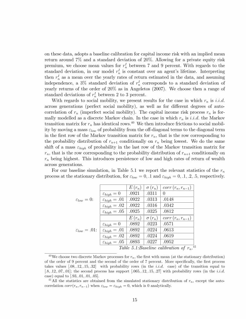
across generations (perfect social mobility), as well as for di¤erent degrees of auto-correlation of rn (imperfect social mobility). The capital income risk process rn is for-mally modelled as a discrete Markov chain. In the case in which rn is i:i:d: the Markovtransition matrix for rn has identical rows.40 We then introduce frictions to social mobil-ity by moving a mass "low of probability from the o¤-diagonal terms to the diagonal termin the �rst row of the Markov transition matrix for rn, that is the row corresponding tothe probability distribution of rn+1 conditionally on rn being lowest. We do the sameshift of a mass "high of probability in the last row of the Markov transition matrix forrn, that is the row corresponding to the probability distribution of rn+1 conditionally onrn being highest. This introduces persistence of low and high rates of return of wealthacross generations.For our baseline simulation, in Table 5:1 we report the relevant statistics of the rn

process at the stationary distribution, for "low = 0; :1 and "high = 0; :1; :2; :5; respectively.

"low = 0:

E (rn) � (rn) corr (rn; rn�1)"high = 0 :0921 :0311 0"high = :01 :0922 :0313 :0148"high = :02 :0922 :0316 :0342"high = :05 :0925 :0325 :0812

"low = :01:

E (rn) � (rn) corr (rn; rn�1)"high = 0 :0892 :0223 :0571"high = :01 :0892 :0224 :0613"high = :02 :0892 :0224 :0619"high = :05 :0893 :0227 :0952

Table 5.1:Baseline calibration of rn:41

40We choose two discrete Markov processes for rn, the �rst with mean (at the stationary distribution)of the order of 9 percent and the second of the order of 7 percent. More speci�cally, the �rst processtakes values [:08; :12; :15; :32] with probability rows (in the i:i:d. case) of the transition equal to[:8; :12; :07; :01]; the second process has support [:065; :12; :15; :27] with probability rows (in the i:i:d.case) equal to [:93; :01; :01; :05]:41All the statistics are obtained from the simulated stationary distribution of rn; except the auto-

correlation corr(rn; rn�1) when "low = "high = 0; which is 0 analytically.

15

Finally, we set the estate tax rate b = 0:2 (which is the average tax rate on bequests),and the capital income tax � = 0:15, in the baseline, but in Section 5.2 we study variouscombinations of �scal policy.With this calibration we simulate the stationary distribution of the economy.42 We

then calculate the top percentiles of the simulated wealth distribution, the Gini coe¢ cientof the whole distribution (not just the "Gini of the tail"), the quintiles, and the tailindex �. While we are mostly concerned with the wealth distribution, we also reportthe capital income to labor income ratio implied in the simulation as an extra check.We aim at a ratio not too distant from :5; the value implied by the standard calibrationof macroeconomic production models (with a constant return to scale Cobb-Douglasproduction function with capital share equal to 1

3): We report �rst, as a baseline, the

case with "low = :01; and various values for "high:First of all, note that the wealth distributions which we obtain in the various simula-

tions in Table 5.2 match quite successfully the top percentiles of the U.S. Furthermore,note that the tail of the simulated wealth distribution economy gets thicker by increasing"high; that is, by increasing corr (rn; rn�1) : In particular, the better �t is obtained withsubstantial imperfections in social mobility ("high = :02); in which case the 99th� 100thpercentile of wealth in the U.S. economy is matched almost exactly.

PercentilesEconomy 90th� 95th 95th� 99th 99th� 100thU:S: :113 :231 :347

"high = 0 :118 :204 :261"high = :01 :116 :202 :275"high = :02 :105 :182 :341"high = :05 :087 :151 :457Table 5.2: Percentiles of the top tail; "low = :01:

More surprisingly, perhaps, the Lorenz curve (in quintiles) of the simulated wealthdistributions, Table 5.3, matches reasonably well that of the U.S.; and so does the Ginicoe¢ cient. Once again, "high = :02 appears to represent the better �t in terms of theLorenz curve and the Gini coe¢ cient (even though the tail index of this calibration islower than the U.S. economy�s, but the tail index is imprecisely estimated with wealthdata).43

42We note under these calibrations of for rn and other parameters, we check that the conditions ofAssumptions 2 and 3 are satis�ed and therefore that the restrictions on � hold.43The calibration with "high = :05; with even more frictions to social mobility, also fares well, though

in this case the tail index is < 1; which implies that the tails are so thick that the theoretical distributionhas no mean. In this case (ii) of Assumption 3 in Appendix B is violated.

16

QuintilesEconomy Tail index � Gini F irst Second Third Fourth F ifthU:S: 1:49 0:803 �:003 :013 0:05 0:122 0:817" = 0 1:796 :646 :033 :058 :08 :123 :707" = 0:01 1:256 :655 :032 :056 :078 :12 :714" = 0:02 1:038 0:685 :029 :051 :071 :11 :739" = 0:05 :716 :742 :024 :042 :058 :09 :786

Table 5.3: Tail Index, Gini, and Quintiles; "low = :01:

Furthermore, the capital income to labor income ratio implied by the simulationstakes on reasonable values: it goes from :3 for " = 0 to :6 for " = :05. In the " = 0:02calibration the capital-labor ratio is almost exactly :5:

5.1 Robustness

As a robustness check, we report the calibration with "low = 0: In this case the simulatedwealth distributions also have Gini coe¢ cients close to that of the U.S. economy andLorenz curves which also match that of the U.S. rather well. Table 5.4 reports the toppercentiles of the U.S. economy and of the simulated wealth distribution.

PercentilesEconomy 90th� 95th 95th� 99th 99th� 100thU:S: :113 :231 :347

"high = 0 :1 :207 :38"high = :01 :082 :173 :49"high = :02 :073 :154 :544"high = :05 :026 :06 :836Table 5.4: Percentiles of the top tail; "low = 0:

Table 5.5 reports instead the tail index, the Gini coe¢ cient, and the Lorenz curve ofthe U.S. economy and of the simulated wealth distribution.44

QuintilesEconomy Tail index � Gini F irst Second Third Fourth F ifthU:S: 1:49 :803 �:003 :013 :05 :122 :817

"high = 0 1:795 :738 :023 :041 :057 :092 :788"high = :01 1:254 :786 :018 :033 :046 :074 :827"high = :02 1:036 :808 :017 :003 :042 :067 :844"high = :05 :713 :933 :006 :01 :014 :023 :947

Table 5.5: Tail Index, Gini, and Quintiles; "low = 0:

44Again, for " = 0:05; we have � < 1: See footnote 43.

17

Note that the calibration with i:i:d: capital income risk rn ("low = "high = 0) doesparticularly well.We also report the simulation for the economy with a di¤erent Markov process for

rn; with pre-tax mean of 7%: Table 5.6 reports the relevant statistics of the rn processat the stationary distribution, in this case, for "low = 0; :1 and "high = :2; respectively.45

"low = 0:E (rn) � (rn) corr (rn; rn�1)

"high = :02 :0772 :0467 :0356

"low = :01:E (rn) � (rn) corr (rn; rn�1)

"high = :02 :0738 :0415 :0542

Table 5.6: Calibration of rn with mean 7%:

Tables 5.7 and 5.8 collect the results regarding the simulated wealth distribution forthis process of capital income risk.

PercentilesEconomy 90th� 95th 95th� 99th 99th� 100thU:S: :113 :231 :347"low = :01; "high = :02 :066 :232 :675"low = 0; "high = :02 :076 :236 :646

Table 5.7: Percentiles of the top tailQuintiles

Economy Tail index � Gini F irst Second Third Fourth F ifthU:S: 1:49 :803 �:003 :013 :05 :122 :817"low = :01; "high = :02 1:514 :993 �:022 :003 :009 :016 :994"low = 0; "high = :02 1:514 :978 �:016 :003 :008 :015 :991

Table 5.8: Tail Index, Gini, and Quintiles

While still in the ballpark of the U.S. economy, these calibrations match it muchmore poorly than the previous ones with a higher mean of rn. Interestingly, thoughthey induce a higher Gini coe¢ cient than in the U.S. distribution, suggesting that ourmodel, in general, does not share the di¢ culties experienced by standard calibratedmacroeconomic models to produce wealth distributions with tails as heavy as thoseobserved in the data.

5.2 Tax experiments

The Tables below illustrate the e¤ects of taxes on the tail index and the Gini coe¢ cient.We calibrate the parameters of the economy, other than b and �, as before, with rn as

45A more extensive set of results is available from the authors upon request.

18

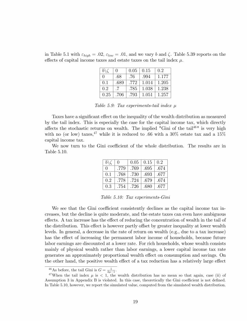
in Table 5.1 with "high = :02; "low = :01; and we vary b and �. Table 5.39 reports on thee¤ects of capital income taxes and estate taxes on the tail index �:

bn� 0 0:05 0:15 0:20 :68 :76 :994 1:1770:1 :689 :772 1:014 1:2050:2 :7 :785 1:038 1:2380:25 :706 :793 1:051 1:257

Table 5.9: Tax experiments-tail index �

Taxes have a signi�cant e¤ect on the inequality of the wealth distribution as measuredby the tail index. This is especially the case for the capital income tax, which directlya¤ects the stochastic returns on wealth. The implied "Gini of the tail46" is very highwith no (or low) taxes,47 while it is reduced to :66 with a 30% estate tax and a 15%capital income tax.We now turn to the Gini coe¢ cient of the whole distribution. The results are in

Table 5.10.

bn� 0 0:05 0:15 0:20 .779 .769 .695 .6740:1 .768 .730 .693 .6770:2 .778 .724 .679 .6740:3 .754 .726 .680 .677

Table 5.10: Tax experiments-Gini

We see that the Gini coe¢ cient consistently declines as the capital income tax in-creases, but the decline is quite moderate, and the estate taxes can even have ambiguouse¤ects. A tax increase has the e¤ect of reducing the concentration of wealth in the tail ofthe distribution. This e¤ect is however partly o¤set by greater inequality at lower wealthlevels. In general, a decrease in the rate of return on wealth (e.g., due to a tax increase)has the e¤ect of increasing the permanent labor income of households, because futurelabor earnings are discounted at a lower rate. For rich households, whose wealth consistsmainly of physical wealth rather than labor earnings, a lower capital income tax rategenerates an approximately proportional wealth e¤ect on consumption and savings. Onthe other hand, the positive wealth e¤ect of a tax reduction has a relatively large e¤ect

46As before, the tail Gini is G = 12��1 :

47When the tail index � is < 1, the wealth distribution has no mean so that again, case (ii) ofAssumption 3 in Appendix B is violated. In this case, theoretically the Gini coe¢ cient is not de�ned.In Table 5.10, however, we report the simulated value, computed from the simulated wealth distribution.

19

for households whose physical wealth is relatively low. These households will smooththeir consumption based on their lifetime labor earnings, and will hence react to a taxreduction by decumulating physical wealth proportionately faster than households thatare relatively rich in physical wealth. As a result of this e¤ect, wealth inequality betweenrich and poor households as measured by physical wealth tends to increase. Of course,the e¤ects of a tax increase on relatively poor households would be moderated (perhapseliminated) if tax revenues were to be redistributed towards the less wealthy.Nonetheless the results of Table 5.10 suggests a word of caution in evaluating the

e¤ects on wealth inequality of proposed �scal policies like the abolition of estate taxesor the reduction of capital taxes. For instance, Castaneda, Diaz Jimenez, and RiosRull (2003) and Cagetti and De Nardi (2007) �nd very small (or even perverse) e¤ectsof eliminating bequest taxes in their calibrations in models with a skewed distributionof earnings but no capital income risk.48 If the capital income risk component is asubstantial fraction of idiosyncratic risk, such �scal policies could have a sizeable e¤ectsin increasing wealth inequality in the top tail of the distribution of wealth which maynot show up in measurements of the Gini coe¢ cient.49

6 Conclusion

The main conclusion of this paper is that capital income risk, that is, idiosyncraticreturns on wealth, has a fundamental role in a¤ecting the distribution of wealth. Capitalincome risk appears crucial in generating the heavy tails observed in wealth distributionsacross a large cross-section of countries and time periods. Furthermore, when the wealthdistribution is shaped by capital income risk, the top tail of wealth distribution is verysensitive to �scal policies, a result which is often documented empirically but hard togenerate in many classes of models without capital income risk. Higher taxes in e¤ectdampen the multiplicative stochastic return on wealth, which is critical to generate theheavy tails.Interestingly, this role of capital income risk as a determinant of the distribution

of wealth seems to have been lost by Vilfredo Pareto. He explicitly noted that anidentical stochastic process for wealth across households will not induce the skewedwealth distribution that we observe in the data (See Pareto (1897), Note 1 to #962,

48See also our discussion of the results of Becker and Tomes (1979), previously in this section.49Empirical studies also indicate that higher and more progressive taxes did in fact signi�cantly reduce

income and wealth inequality in the historical context; notably, e.g., Lampman (1962) and Kuznets(1955). Most recently, Piketty (2001) and Piketty and Saez (2003) have argued that redistributivecapital and estate taxation may have prevented holders of very large fortunes from recovering from theshocks that they experienced during the Great Depression and World War II because of the dynamice¤ects of progressive taxation on capital accumulation and pre-tax income inequality. This line ofargument has been extended to the U.S., Japan, and Canada, respectively, by Moriguchi-Saez (2005),Saez-Veall (2003).

20

p. 315-316). He therefore introduced skewness into the distribution of talents or laborearnings of households (1897, Notes to #962, p. 416). Left with the distribution oftalents and earnings as the main determinant of the wealth distribution, he was perhapslead to his "Pareto�s Law," enunciated e.g., by Samuelson (1965) as follows:

In all places and all times, the distribution of income remains the same. Nei-ther institutional change nor egalitarian taxation can alter this fundamentalconstant of social sciences.50

50See Chipman (1976) for a discussion on the controversy between Pareto and Pigou regarding theinterpretation of the Law. To be fair to Pareto, he also had a "political economy" theory of �scal policy(determined by the controlling elites) which could also explain the "Pareto Law;" see Pareto (1901,1909).

21

References

Aiyagari, S.R. (1994): "Uninsured Idiosyncratic Risk and Aggregate Savings," Quar-terly Journal of Economics,109 (3), 659-684.

Angeletos, G. (2007), "Uninsured Idiosyncratic Investment Risk and Aggregate Saving",Review of Economic Dynamics, 10, 1-30.

Angeletos, G. and L.E. Calvet (2005), "Incomplete-market dynamics in a neoclassicalproduction economy," Journal of Mathematical Economics, 41(4-5), 407-438.

Angeletos, G. and L.E. Calvet (2006), "Idiosyncratic Production Risk, Growth and theBusiness Cycle", Journal of Monetary Economics, 53, 1095-1115.

Arrow, K. (1987): "The Demand for Information and the Distribution of Income,"Probability in the Engineering and Informational Sciences, 1, 3-13.

Atkinson, A.B. (2002): "Top Incomes in the United Kingdom over the Twentieth Cen-tury," mimeo, Nu¢ eld College, Oxford.

Becker, G.S. and N. Tomes (1979): "An Equilibrium Theory of the Distribution ofIncome and Intergenerational Mobility," Journal of Political Economy, 87, 6, 1153-1189.

Benhabib, J. and A. Bisin (2006), "The Distribution of Wealth and RedistributivePolicies", Manuscript, New York University.

Benhabib, J. and S. Zhu (2008): "Age, Luck and Inheritance," NBER Working PaperNo. 14128.

Bertaut, C. and M. Starr-McCluer (2002): "Household Portfolios in the United States",in L. Guiso, M. Haliassos, and T. Jappelli, Editor, Household Portfolios, MIT Press,Cambridge, MA.

Bitler, Marianne P., Tobias J. Moskowitz, and Annette Vissing-Jørgensen (2005): "Test-ing Agency Theory With Entrepreneur E¤ort and Wealth", Journal of Finance,60, 539-576.

Brandt, A. (1986): "The Stochastic Equation Yn+1 = AnYn + Bn with StationaryCoe¢ cients", Advances in Applied Probability, 18, 211�220.

Burris, V. (2000): "The Myth of Old Money Liberalism: The Politics of the "Forbes"400 Richest Americans", Social Problems, 47, 360-378.

Cagetti, C. and M. De Nardi (2005): "Wealth Inequality: Data and Models," FederalReserve Bank of Chicago, W. P. 2005-10.

22

Cagetti, M. and M. De Nardi (2006), "Entrepreneurship, Frictions, and Wealth", Jour-nal of Political Economy, 114, 835-870.

Cagetti, C. and M. De Nardi (2007): "Estate Taxation, Entrepreneurship, andWealth,"NBER Working Paper 13160.

Carroll, C. D. (1997). �Bu¤er-Stock Saving and the Life Cycle/Permanent IncomeHypothesis,�Quarterly Journal of Economics, 112, 1�56.

Castaneda, A., J. Diaz-Gimenez, and J. V. Rios-Rull (2003): "Accounting for the U.S.Earnings and Wealth Inequality," Journal of Political Economy, 111, 4, 818-57.

Champernowne, D.G. (1953): "A Model of Income Distribution," Economic Journal,63, 318-51.

Chipman, J.S. (1976): "The Paretian Heritage," Revue Europeenne des Sciences So-ciales et Cahiers Vilfredo Pareto, 14, 37, 65-171.

Clementi, F. and M. Gallegati (2005): "Power Law Tails in the Italian Personal IncomeDistribution," Physica A: Statistical Mechanics and Theoretical Physics, 350, 427-438.

Dagsvik, J.K. and B.H. Vatne (1999): "Is the Distribution of Income Compatible witha Stable Distribution?," D.P. No. 246, Research Department, Statistics Norway.

De Nardi, M. (2004): "Wealth Inequality and Intergenerational Links," Review of Eco-nomic Studies, 71, 743-768.

Diaz-Gimenez, J., V. Quadrini, and J. V. Rios-Rull (1997): "Dimensions of Inequality:Facts on the U.S. Distributions of Earnings, Income, and Wealth," Federal ReserveBank of Minneapolis Quarterly Review, 21(2), 3-21.

Díaz-Giménez, J., V. Quadrini, J. V. Ríos-Rull, and S. B. Rodríguez (2002): "UpdatedFacts on the U.S. Distributions of Earnings, Income, and Wealth", Federal ReserveBank of Minneapolis Quarterly Review, 26(3), 2-35.

Elwood, P., S.M. Miller, M. Bayard, T. Watson, C. Collins, and C. Hartman (1997):"Born on Third Base: The Sources of Wealth of the 1996 Forbes 400," Boston:Uni�ed for a Fair Economy.

Feenberg, D. and J. Poterba (2000): "The Income and Tax Share of Very High IncomeHousehold: 1960-1995," American Economic Review, 90, 264-70.

Feller, W. (1966): An Introduction to Probability Theory and its Applications, 2, Wiley,New York.

23

Fiaschi, D. and M. Marsili (2009): "Distribution of Wealth and Incomplete Markets:Theory and Empirical Evidence," University of Pisa Working paper 83.

Flavin, M. and T. Yamashita (2002): "Owner-Occupied Housing and the Compositionof the Household Portfolio", American Economic Review, 92, 345-362.

Flodén, M. (2008): "A note on the accuracy of Markov-chain approximations to highlypersistent AR(1) processes" Economics Letters, 99 (3), 2008, 516-520.

Goldie, C. M. (1991): "Implicit Renewal Theory and Tails of Solutions of RandomEquations," Annals of Applied Probability, 1, 126�166.

Guvenen, F. (2007): "Learning Your Earning: Are Labor Income Shocks Really VeryPersistent?," American Economic Review, 97(3), 687-712.

Heathcote, J. (2008): "Discussion Heterogeneous Life-Cycle Pro�les, Income Risk, andConsumption Inequality, by G. Primiceri and T. van Rens," Federal Bank of Min-neapolis, mimeo.

Huggett, M. (1993): "The Risk-Free Rate in Heterogeneous-household Incomplete-Insurance Economies, Journal of Economic Dynamics and Control, 17, 953-69.

Huggett, M. (1996):, "Wealth Distribution in Life-Cycle Economies," Journal of Mon-etary Economics, 38, 469-494.

Kesten, H. (1973): "Random Di¤erence Equations and Renewal Theory for Productsof Random Matrices," Acta Mathematica. 131 207�248.

Klass, O.S., Biham, O., Levy, M., Malcai O., and S. Solomon (2007): "The Forbes 400,the Pareto Power-law and E¢ cient Markets, The European Physical Journal B -Condensed Matter and Complex Systems, 55(2), 143-7.

Krusell, P. and A. A. Smith (1998): "Income and Wealth Heterogeneity in the Macro-economy," Journal of Political Economy, 106, 867-896.

Kuznets, S. (1955): �Economic Growth and Economic Inequality,�American EconomicReview, 45, 1-28.

Lampman, R.J. (1962): The Share of Top Wealth-Holders in National Wealth, 1922-1956, Princeton, NJ, NBER and Princeton University Press.

Levy, M. (2005), " Market E¢ ciency, The Pareto Wealth Distribution, and the LevyDistribution of Stock Returns" in The Economy as an Evolving Complex Systemeds. S. Durlauf and L. Blume, Oxford University Press, USA.

24

Levy, M. and S. Solomon (1996): "Power Laws are Logarithmic Boltzmann Laws,"International Journal of Modern Physics, C,7, 65-72.

Loève, M. (1977), Probability Theory, 4th ed., Springer, New York.

McKay, A. (2008): "Household Saving Behavior, Wealth Accumulation and Social Se-curity Privatization," mimeo, Princeton University.

Meyn, S. and R.L. Tweedie (2009),Markov Chains and Stochastic Stability, 2nd edition,Cambridge University Press, Cambridge.

Moriguchi, C. and E. Saez (2005): "The Evolution of Income Concentration in Japan,1885-2002: Evidence from Income Tax Statistics," mimeo, University of California,Berkeley.

Moskowitz, T. and A. Vissing-Jorgensen (2002): "The Returns to Entrepreneurial In-vestment: A Private Equity Premium Puzzle?", American Economic Review, 92,745-778.

Nirei, M. andW. Souma (2004): "Two Factor Model of Income Distribution Dynamics,"mimeo, Utah State University.

Nishimura, K. and J. Stachurski (2005): "Stability of Stochastic Optimal Growth Mod-els: a New Approach", Journal of Economic Theory, 122, 100-118.

Pareto, V. (1897): Cours d�Economie Politique, II, F. Rouge, Lausanne.

V. Pareto (1901): "Un�Applicazione di teorie sociologiche", Rivista Italiana di So-ciologia. 5. 402-456, translated as The Rise and Fall of Elites: An Applicationof Theoretical Sociology , Transaction Publishers, New Brunswick, New Jersey,(1991).

V. Pareto (1909): Manuel d�Economie Politique, V. Girard et E. Brière, Paris.

Piketty, T. (2003): "Income Inequality in France, 1901-1998," Journal of Political Econ-omy, 111, 1004�42.

Piketty, T. and E. Saez (2003): "Income Inequality in the United States, 1913-1998,"Quarterly Journal of Economics, CXVIII, 1, 1-39.

Quadrini, V. (1999): "The importance of entrepreneurship for wealth concentrationand mobility," Review of Income and Wealth, 45, 1-19.

Quadrini, V. (2000): "Entrepreneurship, Savings and Social Mobility," Review of Eco-nomic Dynamics, 3, 1-40.

25

Panousi, V. (2008): "Capital Taxation with Entrepreneurial Risk," mimeo, MIT.

Primiceri, G. and T. van Rens (2006): "Heterogeneous Life-Cycle Pro�les, Income Risk,and Consumption Inequality," CEPR Discussion Paper 5881.

Roitershtein, A. (2007): "One-Dimensional Linear Recursions with Markov-DependentCoe¢ cients," The Annals of Applied Probability, 17(2), 572-608.

Rutherford, R.S.G. (1955): "Income Distribution: A New Model," Econometrica, 23,277-94.

Saez, E. and M. Veall (2003): "The Evolution of Top Incomes in Canada," NBERWorking Paper 9607.

P.A. Samuelson (1965): �A Fallacy in the Interpretation of the Pareto�s Law of AllegedConstancy of Income Distribution,�Rivista Internazionale di Scienze Economichee Commerciali, 12, 246-50.

Saporta, B. (2004): "Etude de la Solution Stationnaire de l� Equation Yn+1 = anYn+bn,a Coe¢ cients Aleatoires," (Thesis),http://tel.archives-ouvertes.fr/docs/00/04/74/12/PDF/tel-00007666.pdf

Saporta, B. (2005): "Tail of the stationary solution of the stochastic equation Yn+1 =anYn+bn with Markovian coe¢ cients," Stochastic Processes and their Applications,115(12), 1954-1978.

Sornette, D. (2000): Critical Phenomena in Natural Sciences, Berlin, Springer Verlag.

Storesletten, K., C.I. Telmer, and A. Yaron (2004): "Consumption and Risk SharingOver the Life Cycle," Journal of Monetary Economics, 51(3), 609-33.

Tauchen, G. (1986): "Finite State Markov-Chain Approximations to Univariate andVector Autoregressions," Economics Letters, 20(2), 177-81.

Tauchen, G. and R. Hussey (1991): "Quadrature-Based Methods for Obtaining Approx-imate Solutions to Nonlinear Asset Pricing Models," Econometrica, 59(2), 371-96.

Wold, H.O.A. and P. Whittle (1957): "A Model Explaining the Pareto Distribution ofWealth," Econometrica, 25, 4, 591-5.

Wol¤, E. (1987): "Estimates of Household Wealth Inequality in the U.S., 1962-1983,"The Review of Income and Wealth, 33, 231-56.

Wol¤, E. (2004): "Changes in HouseholdWealth in the 1980s and 1990s in the U.S.,"mimeo,NYU.

26

Zhu, S. (2010): "Wealth Distribution under Idiosyncratic Investment Risk", mimeo,NYU.

27

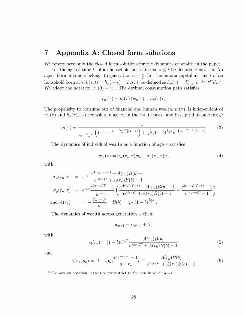
7 Appendix A: Closed form solutions

We report here only the closed form solutions for the dynamics of wealth in the paper.Let the age at time t of an household born at time s � t be denoted � = t� s: An

agent born at time s belongs to generation n = sT: Let the human capital at time t of an

household born at s; h(s; t) = hn(t�s) = hn(�); be de�ned as hn(�) =R T0yne

�(rn�g)�d� .51

We adopt the notation wn(0) = wn: The optimal consumption path satis�es

cn (�) = m(�) (wn(�) + hn(�)) ;

The propensity to consume out of �nancial and human wealth, m(�); is independent ofwn(�) and hn(�), is decreasing in age � ; in the estate tax b; and in capital income tax �:

m(�) =1

1rn� rn��

�

�1� e�(rn�

rn��� )(T��)

�+ �

1� (1� b)

1��� e�(rn�

rn��� )(T��)

(3)

The dynamics of individual wealth as a function of age � satis�es

wn (�) = �w(rn; �)wn + �y(rn; �)yn (4)

with

�w(rn; �) = ern�eA(rn)(T��) + A(rn)B(b)� 1eA(rn)T + A(rn)B(b)� 1

�y(rn; �) = ern�e(g�rn)T � 1g � rn

�eA(rn)(T��) + A(rn)B(b)� 1eA(rn)T + A(rn)B(b)� 1

� e(rn�g)(T��) � 1e(rn�g)T � 1

�and A(rn) = rn �

rn � �

�; B(b) = �

1� (1� b)

1��� :

The dynamics of wealth across generation is then:

wn+1 = �nwn + �n

with

�(rn) = (1� b)ernTA(rn)B(b)

eA(rn)T + A(rn)B(b)� 1(5)

and

�(rn; yn) = (1� b)yne(g�rn)T � 1g � rn

ernTA(rn)B(b)

eA(rn)T + A(rn)B(b)� 1(6)

51For save on notation in the text we restrict to the case in which g = 0:

28

8 Appendix B: Proofs

The stochastic processes for (rn; yn) and the induced processes for (�n; �n)n = (�(rn); �(rn; yn))nare required to satisfy the following assumptions.

Assumption 2 The stochastic process (rn; yn)n is a real, irreducible, aperiodic, station-ary Markov chain with �nite state space �r� �y := fr1; :::; rmg� fy1; :::; ylg . Furthermoreit satis�es:

Pr (rn; yn j rn�1; yn�1) = Pr (rn; yn j rn�1) ;where Pr (rn; yn j rn�1; yn�1) denotes the conditional probability of (rn; yn) given (rn�1; yn�1) :52

A stochastic process (rn; yn)n which satis�es Assumption 2 is a Markov Modulatedchain. This assumption would be satis�ed, for instance, if a single Markov chain, cor-responding e.g., to productivity shocks, drove returns on capital (rn)n ; as well as laborincome (yn)n :

53

Assumption 3 Let P denote the transition matrix of (rn)n: Pii0 = Pr(ri0jri). Let �(�r)denote the state space of (�n)n as induced by the map � (rn) : Then �r, �y and P are suchthat: (i) �r� �y >> 0; ii) P�(�r) < 1; (iii) 9ri such that � (ri) > 1, (iv) Pii > 0; for anyi.

We are now ready to show:

Lemma A. 1 Assumptions 2 on (rn; yn)n imply that (�n; �n)n is a Markov Modulatedchain. Furthermore, Assumption 3 implies that (�n; �n)n is re�ective, that is, it satis�es:(i) (�n; �n)n is > 0; (ii) E (�n j�n�1 ) < 1; for any �n�1; 54 (iii) �i > 1 for somei = 1; :::m, (iv) the diagonal elements of the transition matrix P of �n are positive.

Proof of Lemma A.1. Let A be the diagonal matrix with elements Aii = �i; andAij = 0, j 6= i. Note that E (�n j�n�1 ) ; for any �n�1 can be written as P�(�r) < 1.Let r= fr1; :::; rmg denote the state space of rn: Similarly, let y= fy1; :::; ylg denote thestate space of yn: Let � = f�1; :::�mg and � =

��1; :::�l

denote the state spaces of,

respectively, �n and �n, as they are induced through the maps 5 and 6. We shall showthat the maps 5 and 6 are bounded in rn and yn: Therefore the state spaces of �n and

52While Assumption 2 requires rn to be independent of (yn�1; yn�2:::), it leaves the auto-correlationof (rn)n unrestricted, in the space of Markov chains. Also, Assumption 2 allows for (a restricted formof) auto-correlation of (yn)n as well as the correlation of yn and rn:53 For the use of Markov Modulated chains, see Saporta (2005) in her remarks following Theorem

2, or Saporta (2004), section 2.9, p.80. See instead Roitersthein (2007) for general Markov Modulatedprocesses.54We could only require that the mean of the unconditional distribution of � is less than 1; that is if

E (�) < 1. But in this case the stationary distribution of wealth may not have a mean.

29

�n are well de�ned. It immediately follows then that, if (rn; yn)n is a Markov Modulatedchain (Assumption 2), so is (�n; �n)n.We now show that under Assumption 3 (i), (�n; �n)n is > 0 and bounded with

probability 1 in rn and yn: Recall that B(b) = �1� (1� b)

1��� > 0. Note that

�(rn) = (1� b)B(b)

e�rn���

TR T0e�A(rn)(T�t)dt+ e�rnTB(b)

Therefore �n > 0 and bounded. Furthermore, note that

�(rn; yn) = �(rn)yn

Z T

0

e(g�rn)tdt

and the support of yn is bounded by Assumption 2. Thus (�n)n � 0 and is bounded.Therefore (�n; �n) is a MarkovModulated Process provided (�n)n is positive and bounded.Furthermore, Assumption 3 (ii) implies directly that (ii) P �� < 1: Assumption 3 (iii)

also directly implies �i > 1 for some i = 1; :::m. Finally P is the transition matrix ofboth rn as well as of �n: Therefore Assumption 3 (iv) implies that the elements of thetrace of the transition matrix of �n are positive. �Proof of Theorem 1. We �rst de�ne rigorously the regularity of the Markov Modulatedprocess (�n; �n)n. In singular cases, particular correlations between �n and �n can createdegenerate distributions that eliminate the randomness of wealth. We rule this out bymeans of the following technical regularity conditions:55

The Markov Modulated process (�n; �n)n is regular, that is

Pr (�0x+ �0 = xj�0) < 1 for any x 2 R+

and the elements of the vector �� = fln�1::: ln�mg � Rm+ are not integral multiples ofthe same number.56

Saporta (2005, Proposition 1, section 4.1) establishes that, for �nite Markov chains,

limN!1

E

N�1Yn=0

(��n)�

! 1N

= � (A�P 0) ;where � (A�P 0) is the dominant root of A�P 0.57

55We formulate these regularity conditions on (�n; �n)n, but they can be immediately mapped backinto conditions on the stochastic process (rn; yn)n .56Theorems which characterize the tails of distributions generated by equations with random multi-

plicative coe¢ cients rely on this type of "non-lattice" assumptions from Renewal Theory; see for exampleSaporta (2005). Versions of these assumption are standard in this literature; see Feller (1966).)57Recall that the matrix AP 0 has the property that the i0th column sum equals the expected value

of �n conditional on �n�1 = �i. When (�n)n is i:i:d:, P has identical rows, so transition probabilitiesdo not depend on the state �i: In this case A�P 0 has identical column sums given by E�� and equal to� (A�P 0) :

30

Condition 2 can then be expressed as � (A�P 0) = 1: The Theorem then follows directlyfrom Saporta (2005), Theorem 1, if we show i) that there exists a � that solves � (A�P 0) =1; and that ii) such � is > 1. Saporta shows that � = 0 is a solution to � (A�P 0) = 1;or equivalently to ln (� (A�P 0)) = 0: This follows from A0 = I and P being a stochasticmatrix. Let E� (r) denote the expected value of �n at its stationary distribution (whichexists as it is implied by the ergodicity of (rn)n, in turn a consequence of Assumption2). Saporta, under the assumption E� (r) < 1; shows that d ln�(A�P 0)

��< 0 at � = 0; and

that ln (� (A�P 0)) is a convex function of �.58 Therefore, if there exists another solution� > 0 for ln (� (A�P 0)) = 0; it is positive and unique.To assure that � > 1 we replace the condition E� (r) < 1 with (ii) of Proposition 3,

P �� < 1: This implies that the column sums of AP 0 are < 1: Since AP 0 is positive andirreducible, its dominant root is smaller than the maximum column sum. Therefore for� = 1; � (A�P 0) = � (AP 0) < 1. Now note that if (�n; �n)n is re�ective, by Proposition1, Pii > 0 and �i > 1; for some i:This implies that the trace of A�P 0 goes to in�nity if� does (see also Saporta (2004) Proposition 2.7). But the trace is the sum of the rootsso the dominant root of A�P 0; � (A�P 0) ; goes to in�nity with �. It follows that for thesolution of ln (� (A�P 0)) = 0;we must have � > 1: This proves ii). �Proof of Theorem 2.We �rst show, Lemma A.2, that the process (wn; rn�1)n is ergodic59 and thus has a

unique stationary distribution. If we denote with � the product measure of the stationarydistribution of (wn; rn�1)n, and we denote with � the product measure of the stationarydistribution of (wn; rn)n, the relationship between � and v is

v(dw; rn) =Xrn�1

(Pr(rnjrn�1)�(dw; rn�1)) :

Ergodicity of (wn; rn�1)n then implies ergodicity of (wn; rn)n; which then also has a uniquestationary distribution. Actually, Lemma 1 shows that (wn; rn�1)n is V�uniformlyergodic, which is stronger than ergodicity. For the mathematical concepts such asV�uniform ergodicity, �irreducibility, and petite sets, which we use in the proof, seeMeyn and Tweedie (2005).

Lemma A. 2 The process (wn; rn�1)n is V�uniformly ergodic.

Proof of Lemma A.2. As in Theorem 1,

wn+1 = �(rn)wn + �(rn; yn)

58This follows because limn!11n lnE (�0��1:::�n�1)

�= ln (� (A�P 0)) and because the moments of

non-negative random variables are log-convex (in �); see Loeve(1977), p. 158.59Actually Lemma A.2 shows that

(wn; rn�1)n is V�uniformly ergodic, which is stronger than ergodicity. For these mathematical conceptssuch as V�uniform ergodicity, �irreducibility, and petite sets, see Meyn and Tweedie (2005).

31

As assumed in Theorem 1, the process (rn; yn)n satis�es Assumption 2 and 3.Let �L = mini=1;2;��� ;mf�(ri)g and �L = mini=1;2;��� ;m;j=1;2;��� ;lf�(rn; yn)g. Thus �L

1��L

is the lower bound of the state space of wn. Let X = [ �L

1��L ;+1) � f�r1; � � � ; �rmg.Assumption 2, 3 and the regularity assumption of (�n; �n)n guarantee that the processvisits with positive probability in �nite time a dense subset of its support; see Brandt(1986) and Saporta (2005), Theorem 2, p. 1956. The stochastic process (wn; rn�1)n isthen �irreducible and aperiodic.60Let ~� = maxi=1;2;��� ;mfE(�(rn)j�(ri))g. From (ii) of Lemma 3, we knowE(�nj�n�1) <

1 for any �n�1. Thus ~� < 1. Let w =�U+11�~� where �U = maxi=1;2;��� ;m;j=1;2;��� ;lf�(rn; yn)g.

Let C = [ �L

1��L ; w]� f�r1; � � � ; �rmg. Pick a function V (wn; rn�1) = wn so that

E(V (wn+1; rn)j(wn; rn�1)) = E(wn+1j(wn; rn�1))= E(�(rn)jrn�1)wn + E(�(rn; yn)jrn�1)� wn � 1 +

��U + 1

�IC(wn; rn�1)

= V (wn; rn�1)� 1 +��U + 1

�IC(wn; rn�1)

Thus (wn; rn�1)n satis�es the Drift condition of Tweedie (2001).For a sequence of measurable set Bn with Bn # ?, there are two cases: (i) Bn is

contained in a compact set in X, and (ii) Bn has forms of (xn;+1)� �ri or of the unionof such sets. In both cases it is easy to show that

limn!1

sup(w;r)2C

P ((w; r); Bn) = 0;

where P (�; �) is the one-step transition probability of the stochastic process (wn; rn�1)n.Thus(wn; rn�1)n satis�es the Uniform Countable Additivity condition of Tweedie (2001).As a consequence, (wn; rn�1)n satis�es Condition A of Tweedie (2001). V (wn; rn�1) =

wn is everywhere �nite and (wn; rn�1)n is �irreducible. By Theorem 3 of Tweedie(2001), we know that the set C is petite.61

60Alternatively to the regularity assumption, we could assume a continuous distribution for yn (andhence for �n): Irreducibility would then easily follow; see Meyn-Tweedie (2009), p. 76.61Note that (1) Every subset of a petite set is petite; and (2) When we pick any w, such that w > �U+1

1�~�to replace w, the proof goes through. By these two facts we could show that every compact set of X ispetite. Thus by Theorem 6.2.5 of Meyn and Tweedie (2009) we know that (wn; rn�1)n is a T�chain.For another example of stochastic process in economics with the property that every compact set ispetite, see Nishimura and Stachurski (2005).

32

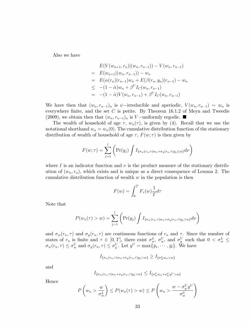
Also we have

E(V (wn+1; rn)j(wn; rn�1))� V (wn; rn�1)

= E(wn+1j(wn; rn�1))� wn

= E(�(rn)jrn�1)wn + E(�(rn; yn)jrn�1)� wn

� �(1� �)wn + �UIC(wn; rn�1)

= �(1� �)V (wn; rn�1) + �UIC(wn; rn�1)

We have then that (wn; rn�1)n is �irreducible and aperiodic, V (wn; rn�1) = wn iseverywhere �nite, and the set C is petite. By Theorem 16.1.2 of Meyn and Tweedie(2009), we obtain then that (wn; rn�1)n is V�uniformly ergodic. �The wealth of household of age � ; wn(�), is given by (4). Recall that we use the

notational shorthand wn = wn(0): The cumulative distribution function of the stationarydistribution of wealth of household of age � , F (w; �) is then given by

F (w; �) =lX

j=1

�Pr(yj)

ZIf�w(rn;�)wn+�y(rn;�)yj�wgd�

�where I is an indicator function and � is the product measure of the stationary distrib-ution of (wn; rn), which exists and is unique as a direct consequence of Lemma 2. Thecumulative distribution function of wealth w in the population is then

F (w) =

Z T

0

F� (w)1

Td�

Note that

P (wn(�) > w) =lX

j=1

�Pr(yj)

ZIf�w(rn;�)wn+�y(rn;�)yj>wgd�

�and �w(rn; �) and �y(rn; �) are continuous functions of rn and � . Since the number ofstates of rn is �nite and � 2 [0; T ], there exist �Lw, �Uw , and �Uy such that 0 < �Lw ��w(rn; �) � �Uw and �y(rn; �) � �Uy . Let y

U = maxf�y1; � � � ; �ylg. We have

If�w(rn;�)wn+�y(rn;�)yj>wg � If�Lwwn>wg

andIf�w(rn;�)wn+�y(rn;�)yj>wg � If�Uwwn+�Uy yU>wg

Hence

P

�wn >

w

�Lw

�� P (wn(�) > w) � P

wn >

w � �Uy yU

�Uw

!

33

We have then

1� F (w) =

Z T

0

P (wn(�) > w)1

Td�:

Thus

P

�wn >

w

�Lw

�� 1� F (w) � P

wn >

w � �Uy yU

�Uw

!;

and ��Lw��k � lim inf

w!+1

1� F (w)

w��� lim sup

w!+1

1� F (w)

w�����Uw��k

since limw!+1P (wn>w)w�� = k. We conclude that the wealth distribution in the population

has a power tail with the same exponent �, i.e.,

0 < k1 � lim infw!+1

1� F (w)

w��� lim sup

w!+1

1� F (w)

w��� k2: �

We can also show that,When (rn)n is i:i:d:, the asymptotic power law property with the same power � is

preserved for each age cohort and the whole economy: 9~k > 0 such that

limw!+1

1� F (w)

w��= ~k:

Proof. When (rn)n is i:i:d:

1� F (w) =

Z T

0

P (wn(�) > w)1

Td�

=mXi=1

lXj=1

�Pr(ri) Pr(yj)

Z T

0

P

�wn >

w � �y(ri; �)yj�w(ri; �)

�1

Td�

�Since �w(ri; �) and �y(ri; �) are continuous functions of � on [0; T ], there exist ~� i, � i 2[0; T ] such that for 8t 2 [0; T ], �w(ri; �) � �w(ri; ~� i) and �y(ri; �) � �y(ri; � i). Thus

P

�wn >

w � �y(ri; �)yj�w(ri; �)

�� P

�wn >

w � �y(ri; � i)yj�w(ri; ~� i)

�When w is su¢ ciently large,

P�wn >

w��y(ri;� i)yj�w(ri;~� i)

�w��

is bounded,

34

since limw!+1P (wn>w)w�� = c. Thus by the bounded convergence theorem, we have

limw!+1

Z T

0

P�wn >

w��y(ri;�)yj�w(ri;�)

�w��

1

Td� =

Z T

0

limw!+1

P�wn >

w��y(ri;�)yj�w(ri;�)

�w��

1

Td�

Thus

limw!+1

1� F (w)

w��=

mXi=1

lXj=1

0@Pr(ri) Pr(yj)Z T

0

limw!+1

P�wn >

w��y(ri;�)yj�w(ri;�)

�w��

1

Td�

1A= k

mXi=1

�Pr(ri)

Z T

0

(�w(ri; �))� d�

�: �

Proof of Proposition 1. Since � > 1, (�n)� is an increasing convex function in

�n. If �(rn) is a convex function of rn, then �(rn)� is also a convex function of rn. Andhence ��(rn)� is a concave function of rn. By the second order stochastic dominance wehave E (��(rn)�) � E (��(r0n)�) so E�(rn)� � E�(r0n)

� and 1 = E�(rn)� � E�(r0n)

�.Let �0 solve E�(r0n)

�0 = 1. Suppose �0 > �. By Holder�s inequality we have E�(r0n)� <�

E�(r0n)~�� ��0 = 1. This is a contradiction. Thus we have �0 � �. �

Proof of Proposition 2. From the de�nition of �n, we have

�(rn) =(1� b)ernT

��1� (1� b)

��1�R T0eA(rn)tdt+ 1

it is easy to show that @�n@�

> 0:Thus an in�nitesimal increase in � shifts the state spacea to the right. Therefore elements of the non-negative matrix [A�P 0] increase, whichimplies that the dominant root � (A�P 0) is increases. However we know from Saporta(2005) that ln (� (A�P 0)) is a convex function of �:62 At � = 0 it is equal to zero, sinceA0 is the identity matrix and P is a stochastic matrix with dominant root equal to unity.At � = 0 the function ln (� (A�P 0)) is also decreasing. (See Saporta (2005), Proposition2, p.1962.) Then ln (� (A�P 0)) must be increasing at the positive value of � which solvesln� (A�P 0) = 0: Therefore to preserve ln (� (A�P 0)) = 0, � must decline. �Proof of Proposition 3. From (5), we have

�(rn) =ernT

��1� (1� b)�

1�R T0eA(rn)tdt+ (1� b)�1

Thus @�n@b

< 0. To see @�n@�

< 0, we rewrite the expression of �(rn) as

�(rn) = (1� b)B(b)

e�rn���

TR T0e�A(rn)(T�t)dt+ e�rnTB(b)

62See Loeve (1977), page 158.

35

Note that A(rn) = rn � rn���and B(b) = �

1� (1� b)

1��� . @A(rn)

@rn= ��1

�� 0, since � � 1

by Assumption 1. And also B(b) > 0. Thus @�n@rn

> 0. Higher � means lower rn. We have@�n@�

< 0. Now the proof is identical to the proof of Proposition 2 in the reverse directionsince @�n

@b< 0 and @�n

@�< 0 whereas @�n

@�> 0. �

Proof of Proposition 4. From

ln�n = �n + ��n�1

we havenXt=1

ln�t = ��0 + �n +

n�1Xt=1

(1 + �)�t

Thus

limn!+1

1

nln

E

nYt=1

�t

!�!= lim

n!+1

1

nln�Ee�

Pnt=1 ln�t

�=

limn!+1

1

nlnEe�

Pn�1t=1 (1+�)�t = lim

n!+1

1

n

n�1Xt=1

lnEe�(1+�)�t =

limn!+1

1

n

n�1Xt=1

lnEe�(1+�)�t = lnEe�(1+�)�t

Thus limn!+11nln

E

nYt=1

�t

!�!= 0 implies

Ee�(1+�)�t = 1:

Consider in turn the case in which

ln�n = � ln�n�1 + �n:

We havenXt=1

ln�t =�(1� �n)

1� �ln�0 +

nXt=1

1� �n�t+1

1� ��t

Thus

limn!+1

1

nln

E

nYt=1

�t

!�!= lim

n!+1

1

nln�Ee�

Pnt=1 ln�t

�=

limn!+1

1

nln

�Ee�

Pnt=1

1��n�t+11�� �t

�= lim

n!+1

1

n

nXt=1

ln

�Ee

1��n�t+11�� ��t

�= ln

�Ee

11����t

�36

Thus limn!+11nln

E

nYt=1

�t

!�!= 0 implies

Ee�1�� �t = 1: �

37