The Displacement Effect of

Compulsory Pension Savings on

Private Savings

Evidence from the Netherlands, Using

Institutional Differences across

Occupations Yue Li, Rik Dillingh and Mauro Mastrogiacomo

DP 08/2016-025

1

The displacement effect of compulsory pension

savings on private savings. Evidence from the

Netherlands, using institutional differences

across occupations

Yue Li (VU University of Amsterdam), Rik Dillingh (Tilburg University, Dutch

Ministry of Social Affairs and Employment), Mauro Mastrogiacomo (De

Nederlandsche Bank, VU University of Amsterdam)

August 5th 2016

Abstract

We study the displacement effect of mandatory occupational pension saving on private household wealth

in the Netherlands, separately for wage-employed and self-employed. We use rich administrative data

on (pension) wealth and income and apply a range of identification strategies, from IV regressions

to propensity score matching and difference-in-differences analyses, to determine the displacement

effects. To the best of our knowledge, for the first time, we merge pension funds balance sheet data

to the micro data of their members. We set up a quasi-natural experiment, based on the differential

impact of the financial crisis on the separate pension funds in the Netherlands, and we find that those

whose pension fund did not need to apply a recovery plan accumulated about 3,500 euro less

household wealth over de period 2007-2010. Our preferred regression analyses on couples show a

displacement effect of -33% for wage-employed and a higher one of -61% for self-employed. Self-

employed are arguably more aware of their pension accrual, or lack thereof, because they are

responsible for the payment of their pension premiums. Also, the self-employed are on average less

risk-averse than wage-employed, and can thus be expected to hold less precautionary savings.

Keywords: Displacement effect, pension wealth, savings, occupation, balance sheet data.

JEL Classification: D91, E21

2

1 Introduction

A mandatory retirement system, for instance in the form of social security, occupational

pension or any other compulsory scheme, can affect private savings through the displacement

effect, and by inducing early retirement (Feldstein, 1974). The effects on early retirement

have been extensively documented by e.g. Gruber and Wise (1999, 2008). Our paper

further investigates the displacement effect of obligatory pension savings on private

(discretionary) savings. More information on the displacement effect – and the heterogeneity

thereof – can be of guidance to policy makers who are looking for ways to help vulnerable

groups better prepare for retirement or to make the pension system more robust in light of

an ageing society.

Many studies have appeared on this subject, resulting in a wide range of estimates for the

displacement effect. This large variety in outcomes reflects the heterogeneity among the

research subjects. The studies vary, for example, in the periods, the countries and the

pension schemes (public and/or private) they examine. But this type of research is also

often plagued by biases and measurement error. Especially pension wealth is notorious for

its elusiveness. So, part of the deviation in estimates will stem from the different data sets

and estimation strategies that have been used. Each strategy and study has specific strengths

and draw-backs.

Our paper adds to the existing literature on several accounts. We explore new rich

administrative datasets on pension participation and on pension wealth in the Netherlands,

and take into account the differences in institutions related to occupational choice and income

levels. This allows us to assess the displacement effect also for the self-employed and

compare this to the displacement effect for the wage-employed. Based on possible differences

in awareness of the accumulation of pension rights and in risk aversion between these groups,

we would expect to find higher displacement effects for self-employed than for wage-

employed. We also link balance sheet data of pension funds to our micro data, for workers

in several binding labor agreements, which allows us to set up a quasi-natural experiment.

We use standard estimation techniques, but we also explore instrumental variables, propensity

score matching and difference-in-differences techniques to identify the (heterogeneity in the)

displacement effect and check the robustness of our findings.

The results of our quasi-natural experiment indicate that those whose pension fund did not

need to apply a recovery plan accumulated about 3,500 euro less household wealth over de

period 2007-2010. Our preferred regression analyses further show an average displacement

effect for couples of -33% for wage-employed and of -61% for self-employed. Propensity

score matching and difference-in-differences analyses confirm the existence of substantial

displacement effects, though not all estimates are significant.

3

We will start with discussing some of the more recent and influential papers on the

displacement effect in Section 2. We include several papers on Dutch data, because our

empirical analysis is focused on the Netherlands, due to data availability and the possibility

to exploit a quasi-natural experiment. We present a structural model in Section 3. Section

4 contains a description of our data sources and in Section 5, on the empirical implementation,

we describe our identification strategies. Section 6 shows our primary results and we conclude

in Section 7.

2 Literature overview

Attanasio and Brugiavini (2003) provided one of the first micro-based studies of the

displacement effect, which they identify using the 1992 Italian pension reform. They exploit

the variability in exogenous changes in pension wealth across groups of Italian households to

identify the effect that pension wealth has on saving rates. Based on estimated pension

wealth they find a displacement effect of -35% on average, but close to -100% for workers

aged between 35 and 45. Attanasio and Rohwedder (2003) perform a comparable analysis

using UK pension reforms over the period 1975-1981, with comparable results. They find

substantial displacement effects (–55% to –75%), primarily among the older and higher

income households. They state that the lower displacement among the poorer and younger

households might be caused by liquidity constraints.

Engelhardt and Kumar (2011) study the 1992 wave of the US Health and Retirement Study

to estimate the displacement effect. They reduce measurement error by constructing an

instrumental variable, based on employer-provided pension wealth and Social Security wealth,

and find a displacement effect of about –60%, while their original OLS estimate is +23%.

Half of the difference is due to bias from measurement errors in pension wealth in the OLS

estimate. The other half is due to nonlinearities and unobserved heterogeneity. They also find

that displacement is higher at the higher wealth quantiles.

Using a large Danish panel data set over the period 1995 to 2009, Chetty et al. (2014)

show that the effects of retirement savings policies on wealth accumulation depend on whether

they change savings rates by active or passive choice. They find that approximately 85% of

individuals are passive savers who save more when induced to do so by an automatic

contribution, but do not respond at all to price subsidies. Such subsidies lead to little action

at all and, if so, than primarily by individuals who are planning and saving for retirement

already and who respond by basically shifting savings across accounts, which leads to almost

full displacement.

4

Kapteyn and Panis (2005) look at differences in the generosity of pension schemes between

the USA, Italy and the Netherlands. They find that on average the replacement rate in the

USA is substantially lower than in the Netherlands, but this can be compensated almost fully

by annuitizing net wealth, which is substantially larger in de USA. They conclude that this is

fully consistent with a life-cycle model, where the relatively large institutional pension savings

in the Netherlands have displaced personal retirement savings. Hurd et al. (2012) use

micro-data sets from 12 countries to construct income replacement rate and private saving

measures by education level and marital status, as proxies for lifetime earnings. They estimate

the displacement effect by using cross-country differences in the progressivity of the pension

formula and the average generosity and find that an extra dollar of public pension displaces

22 cents of accumulated financial assets. Both studies face the challenge of comparing

countries with potentially considerable institutional and cultural differences. Job and pension

scheme characteristics may differ across and within countries because of institutional features,

such as the Italian credit restrictions mentioned by Kapteyn and Panis (2005). Alessie et

al. (2013) estimate the displacement effect for 13 European countries, including the

Netherlands, based on SHARELIFE data. Their data include retrospective data on lifetime

earnings. Their robust (median) regression results suggest a displacement effect of 47 (61)

percent. They also explore IV estimates, which suggest full displacement, but with less

precision.

Euwals (2000) and Kapteyn et al. (2005) focus specifically on the case of the Netherlands.

Euwals (2000) exploits the heterogeneity in occupational pension wealth within a Dutch

survey dataset from 1994 to explain differential savings. His dataset does not allow him to

make an accurate quantitative estimate of the displacement effect, but he does find a

significant negative impact of both social security and pension wealth on savings motives with

respect to old age. Kapteyn et al. (2005) study the differential impact of the introduction

of the social security system in the Netherlands on the wealth holdings of separate cohorts,

in order to identify the displacement effect of social security on private wealth. They show

that an increase in social security benefit by 1,000 guilders reduces net worth by 115

guilders, thus finding a displacement effect of -11.5%. One reason they mention for finding

a relatively low level of displacement is the potential effect of social security on earlier

retirement, which increases the need to save, and hence attenuates the effect of social

security on saving.

5

3 The model

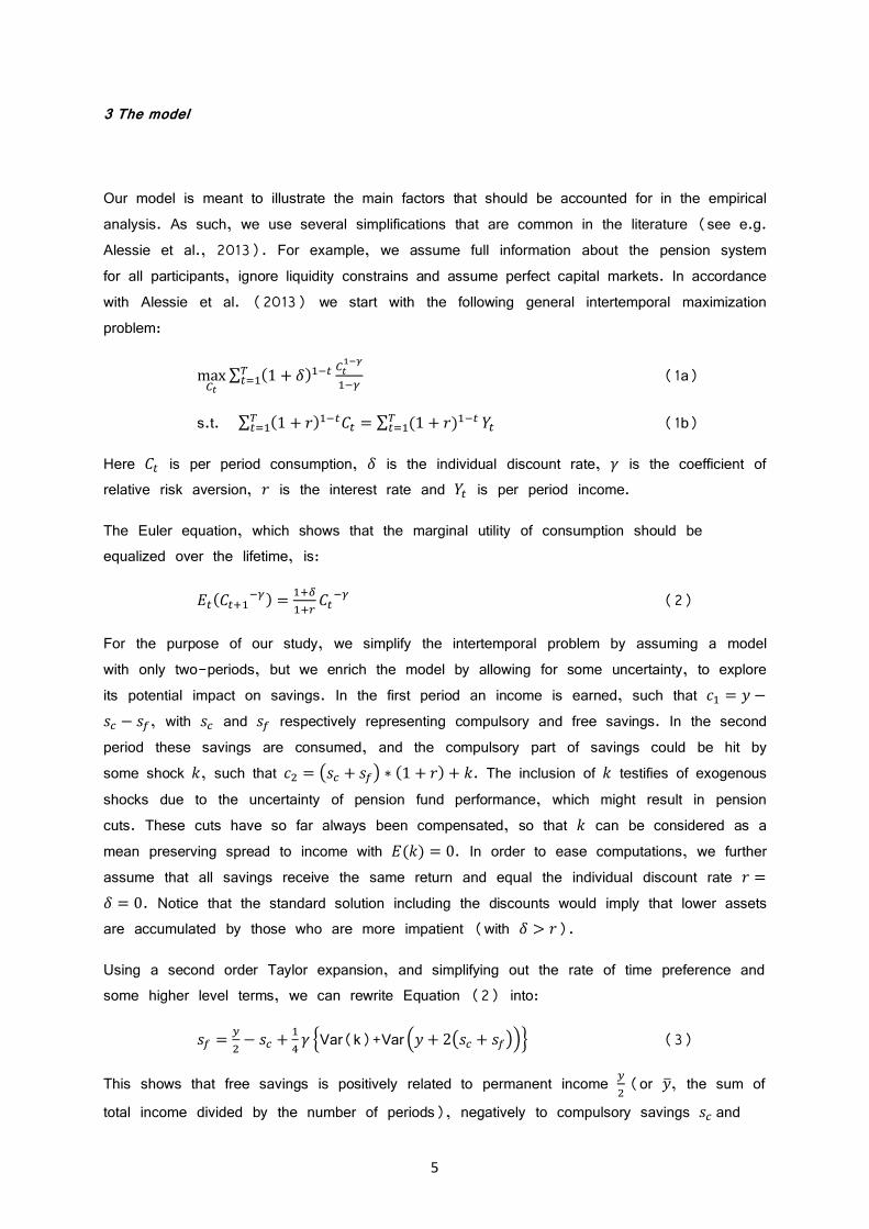
Our model is meant to illustrate the main factors that should be accounted for in the empirical

analysis. As such, we use several simplifications that are common in the literature (see e.g.

Alessie et al., 2013). For example, we assume full information about the pension system

for all participants, ignore liquidity constrains and assume perfect capital markets. In accordance

with Alessie et al. (2013) we start with the following general intertemporal maximization

problem:

max��∑ �1 + �� �����

�����

� � (1a)

s.t. ∑ �1 + ��� ��� = ∑ �1 + ��� ����� ���

��� (1b)

Here �� is per period consumption, is the individual discount rate, � is the coefficient of relative risk aversion, � is the interest rate and �� is per period income.

The Euler equation, which shows that the marginal utility of consumption should be

equalized over the lifetime, is:

������� �� = ������ ��

� (2)

For the purpose of our study, we simplify the intertemporal problem by assuming a model

with only two-periods, but we enrich the model by allowing for some uncertainty, to explore

its potential impact on savings. In the first period an income is earned, such that �� = � −!" − !#, with !" and !# respectively representing compulsory and free savings. In the second

period these savings are consumed, and the compulsory part of savings could be hit by

some shock $, such that �% = &!" + !#' ∗ �1 + �� + $. The inclusion of $ testifies of exogenous shocks due to the uncertainty of pension fund performance, which might result in pension

cuts. These cuts have so far always been compensated, so that $ can be considered as a mean preserving spread to income with ��$� = 0. In order to ease computations, we further

assume that all savings receive the same return and equal the individual discount rate � = = 0. Notice that the standard solution including the discounts would imply that lower assets

are accumulated by those who are more impatient (with > �).

Using a second order Taylor expansion, and simplifying out the rate of time preference and

some higher level terms, we can rewrite Equation (2) into:

!# = +% − !" +

�, � -Var(k)+Var .� + 2&!" + !#'01 (3)

This shows that free savings is positively related to permanent income +%(or �3, the sum of

total income divided by the number of periods), negatively to compulsory savings !" and

6

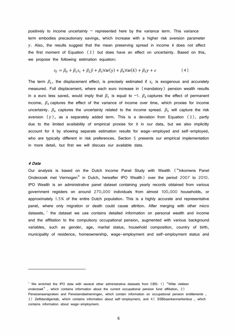
positively to income uncertainty – represented here by the variance term. This variance

term embodies precautionary savings, which increase with a higher risk aversion parameter

�. Also, the results suggest that the mean preserving spread in income k does not affect

the first moment of Equation (3) but does have an effect on uncertainty. Based on this,

we propose the following estimation equation:

!# = 45 + 4�!" + 4%�3 + 46Var��� + 4,Var�$� + 47� + 8 (4)

The term 4�, the displacement effect, is precisely estimated if !" is exogenous and accurately measured. Full displacement, where each euro increase in (mandatory) pension wealth results

in a euro less saved, would imply that 4� is equal to –1. 4%captures the effect of permanent

income, 46captures the effect of the variance of income over time, which proxies for income

uncertainty. 4, captures the uncertainty related to the income spread. 47 will capture the risk aversion (�), as a separately added term. This is a deviation from Equation (3), partly

due to the limited availability of empirical proxies for it in our data, but we also implicitly

account for it by showing separate estimation results for wage-employed and self-employed,

who are typically different in risk preferences. Section 5 presents our empirical implementation

in more detail, but first we will discuss our available data.

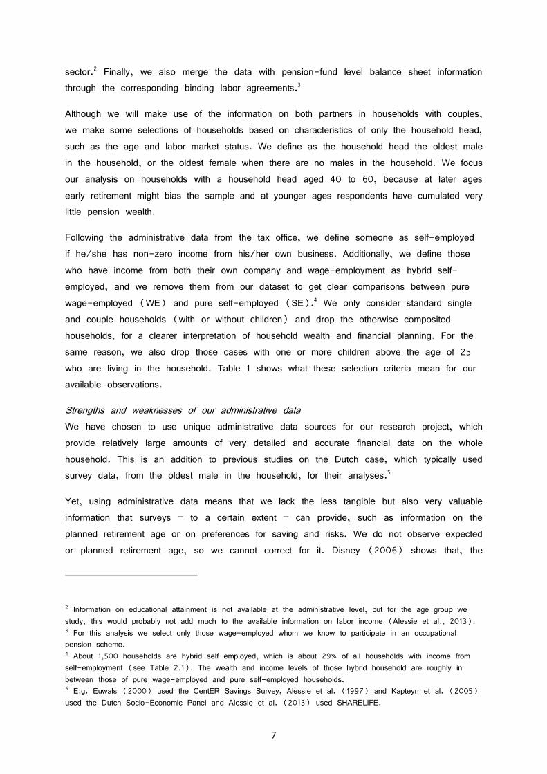
4 Data

Our analysis is based on the Dutch Income Panel Study with Wealth (“Inkomens Panel

Onderzoek met Vermogen” in Dutch, hereafter IPO Wealth) over the period 2007 to 2010.

IPO Wealth is an administrative panel dataset containing yearly records obtained from various

government registers on around 270,000 individuals from almost 100,000 households, or

approximately 1.5% of the entire Dutch population. This is a highly accurate and representative

panel, where only migration or death could cause attrition. After merging with other micro

datasets, 1 the dataset we use contains detailed information on personal wealth and income

and the affiliation to the compulsory occupational pension, augmented with various background

variables, such as gender, age, marital status, household composition, country of birth,

municipality of residence, homeownership, wage-employment and self-employment status and

1 We enriched the IPO data with several other administrative datasets from CBS: 1) “Witte vlekken

onderzoek” , which contains information about the current occupational pension fund affiliation, 2)

Pensioenaanspraken and Pensioendeelnemingen, which contain information on occupational pension entitlements ,

3) Zelfstandigentab, which contains information about self-employment, and 4) SSBbaankenmerkenbus , which

contains information about wage-employment.

7

sector.2 Finally, we also merge the data with pension-fund level balance sheet information

through the corresponding binding labor agreements.3

Although we will make use of the information on both partners in households with couples,

we make some selections of households based on characteristics of only the household head,

such as the age and labor market status. We define as the household head the oldest male

in the household, or the oldest female when there are no males in the household. We focus

our analysis on households with a household head aged 40 to 60, because at later ages

early retirement might bias the sample and at younger ages respondents have cumulated very

little pension wealth.

Following the administrative data from the tax office, we define someone as self-employed

if he/she has non-zero income from his/her own business. Additionally, we define those

who have income from both their own company and wage-employment as hybrid self-

employed, and we remove them from our dataset to get clear comparisons between pure

wage-employed (WE) and pure self-employed (SE).4 We only consider standard single

and couple households (with or without children) and drop the otherwise composited

households, for a clearer interpretation of household wealth and financial planning. For the

same reason, we also drop those cases with one or more children above the age of 25

who are living in the household. Table 1 shows what these selection criteria mean for our

available observations.

Strengths and weaknesses of our administrative data

We have chosen to use unique administrative data sources for our research project, which

provide relatively large amounts of very detailed and accurate financial data on the whole

household. This is an addition to previous studies on the Dutch case, which typically used

survey data, from the oldest male in the household, for their analyses.5

Yet, using administrative data means that we lack the less tangible but also very valuable

information that surveys – to a certain extent – can provide, such as information on the

planned retirement age or on preferences for saving and risks. We do not observe expected

or planned retirement age, so we cannot correct for it. Disney (2006) shows that, the

2 Information on educational attainment is not available at the administrative level, but for the age group we

study, this would probably not add much to the available information on labor income (Alessie et al., 2013). 3 For this analysis we select only those wage-employed whom we know to participate in an occupational

pension scheme. 4 About 1,500 households are hybrid self-employed, which is about 29% of all households with income from

self-employment (see Table 2.1). The wealth and income levels of those hybrid household are roughly in

between those of pure wage-employed and pure self-employed households. 5 E.g. Euwals (2000) used the CentER Savings Survey, Alessie et al. (1997) and Kapteyn et al. (2005)

used the Dutch Socio-Economic Panel and Alessie et al. (2013) used SHARELIFE.

8

more actuarially fair the pension scheme is, the more it will lead to the displacement of

private assets and the less it will result in changes in the retirement age. The Dutch

occupational pensions became substantially more actuarially fair since new legislation in 2006

largely abolished (the explicit or implicit subsidies on) early retirement schemes.6 Still, other

redistributive elements within the Dutch pension system have remained.

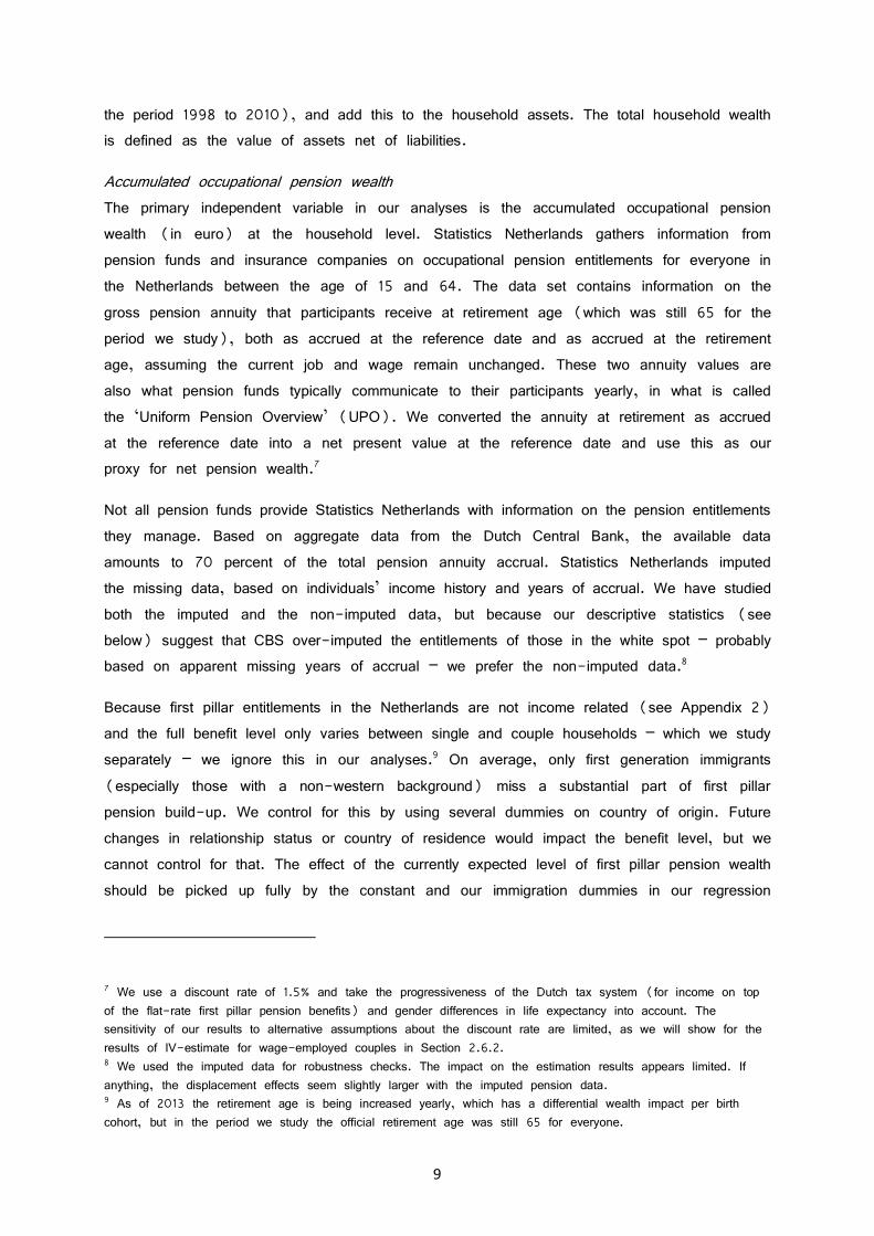
Table 1: Selection criteria and available number of observations

Selection criteria N

Number of households from IPO Wealth panel 95,016

Selection on age of household head: 40-60 41,090

Selection on labor market status household head: WE and/or SE 33,793

Selection on labor market status household head: WE or SE (=dropping hybrids) 32,259

Selection of standard households, loss due to merging datasets, etc. a 28,511

o/w WE couple households 20,616

o/w WE single households 4,085

o/w SE couple households 3,402

o/w SE single households 408

Notes: a We drop households composed of more than one family and those with children above 25 still living in the

household. We also drop the top and bottom 1% for household wealth, household occupation pension wealth and household

income. Additionally, there is some loss of observations due to merging with other datasets.

The saving propensity and relative risk-aversion of individuals is also not observed in our

data. We partly correct for the between-group heterogeneity by separating the analyses by

institutional setting (WE vs SE), which is correlated with these preferences. We will also

use dummies for having stocks, for having third pillar pension savings and for homeownership,

to approximate relative risk-aversion and saving preference within the groups.

Household wealth

The primary dependent variable in our analyses is household wealth (in euro). Table 8 in

Appendix 1 lists the composition of private wealth, at the household level. Financial wealth

is the sum of checking accounts and savings accounts, bonds and stocks, minus financial

liabilities. The net value of housing wealth and business equity are available too. Additionally,

we make extrapolations for the savings in private commercial (third pillar) pension products,

based on the available historical information on the premiums paid to these products (over

6 Since 2006 there has been a strong increase of the average effective retirement age for wage-employed

from 61 year in 2006 to 64 year in 2014. Meanwhile, the average effective retirement age for self-employed

remained almost stable at slightly above 66 year over that period. (Statistics Netherlands, January 2015)

9

the period 1998 to 2010), and add this to the household assets. The total household wealth

is defined as the value of assets net of liabilities.

Accumulated occupational pension wealth

The primary independent variable in our analyses is the accumulated occupational pension

wealth (in euro) at the household level. Statistics Netherlands gathers information from

pension funds and insurance companies on occupational pension entitlements for everyone in

the Netherlands between the age of 15 and 64. The data set contains information on the

gross pension annuity that participants receive at retirement age (which was still 65 for the

period we study), both as accrued at the reference date and as accrued at the retirement

age, assuming the current job and wage remain unchanged. These two annuity values are

also what pension funds typically communicate to their participants yearly, in what is called

the ‘Uniform Pension Overview’ (UPO). We converted the annuity at retirement as accrued

at the reference date into a net present value at the reference date and use this as our

proxy for net pension wealth.7

Not all pension funds provide Statistics Netherlands with information on the pension entitlements

they manage. Based on aggregate data from the Dutch Central Bank, the available data

amounts to 70 percent of the total pension annuity accrual. Statistics Netherlands imputed

the missing data, based on individuals’ income history and years of accrual. We have studied

both the imputed and the non-imputed data, but because our descriptive statistics (see

below) suggest that CBS over-imputed the entitlements of those in the white spot – probably

based on apparent missing years of accrual – we prefer the non-imputed data.8

Because first pillar entitlements in the Netherlands are not income related (see Appendix 2)

and the full benefit level only varies between single and couple households – which we study

separately – we ignore this in our analyses.9 On average, only first generation immigrants

(especially those with a non-western background) miss a substantial part of first pillar

pension build-up. We control for this by using several dummies on country of origin. Future

changes in relationship status or country of residence would impact the benefit level, but we

cannot control for that. The effect of the currently expected level of first pillar pension wealth

should be picked up fully by the constant and our immigration dummies in our regression

7 We use a discount rate of 1.5% and take the progressiveness of the Dutch tax system (for income on top

of the flat-rate first pillar pension benefits) and gender differences in life expectancy into account. The

sensitivity of our results to alternative assumptions about the discount rate are limited, as we will show for the

results of IV-estimate for wage-employed couples in Section 2.6.2. 8 We used the imputed data for robustness checks. The impact on the estimation results appears limited. If

anything, the displacement effects seem slightly larger with the imputed pension data. 9 As of 2013 the retirement age is being increased yearly, which has a differential wealth impact per birth

cohort, but in the period we study the official retirement age was still 65 for everyone.

10

analyses and should not impact the relationship between occupation pension wealth and total

private household wealth.

Current pension scheme participation

For several alternative identification strategies, which will be explained in the next section, we

also want to look at the current pension scheme participation status of the households we

study. The pension scheme participation status – and thus also the accumulated amount of

pension wealth – strongly depends on occupational choice. This is why we need to examine

the displacement effect for wage-employed and self-employed separately. Yet, while most

Dutch wage-employed are affiliated to the compulsory occupational pension system (we call

this group WEP: Wage-Employed with compulsory Pension) and most self-employed are not

(we call this group SEN: Self-Employed with No compulsory pension), this relationship is

not 100%. Both groups include a substantial minority with a divergent pension regime.

Among wage-employed there is a largely invisible group in both official statistics and academic

studies, who do not participate in a mandatory pension scheme (we call this group WEN:

Wage-Employed with No compulsory pension). This group is so invisible that in the

Netherlands it is called the white spot (“witte vlek”), as it leaves no mark on paper. To

distinguish between WEP and WEN, we use unique data from the Dutch statistical bureau

(CBS) on the white spot in the Netherlands over the period 2007-2010. On average, their

data showed that in 2010 about 9% of all male employees aged 25-64 did not participate

in an occupational pension scheme. The white spot is relatively larger among those with an

income that is over about twice the median income (15%), those working in the commercial

service sector (15%) or those working at a small company (21% for companies with less

than 10 employees, 6% for companies with over 100 employees).10

At the same time, a proportion of self-employed, who are often mentioned for their lack of

affiliation to the occupational pension system, do actually participate in a mandatory professional

or industry pension fund (we call this group SEP: Self-Employed with compulsory Pension).

For instance medical specialists, general practitioners, physiotherapists, notaries and a group

of painters and carpenters (see Appendix 2 for more details). We identify the SEP by using

the code on the industry in which the self-employed is active (the SBI-code). Participation

in the industry pension fund for painters, carpenters and glaziers is explicitly obliged for those

self-employed active in a specific sector (SBI-code 4334). For the other groups of SEP

their profession is precisely enough defined for us to be sufficiently confident that the

professional pension fund obligation applies to them.

10 Mooij, M. de, A. Dill, M. Geerdinck and E. Vieveen (2012). Witte vlek op pensioengebied 2010. Centraal Bureau voor de Statistiek, Den Haag/Heerlen

11

Descriptive statistics

Table 9a in Appendix 3 compares (for couples) the means and medians of a number of

wealth and income related variables between WEP and WEN and between SEP and SEN

over the year 2010. Table 9c shows our available set of control variables, for both the

household head and the partner. Both tables also report the total number of observations for

each of the four groups in our dataset. First, we notice that in our dataset there are around

9% wage-employed who are not affiliated to the occupational pension system, and around

7% self-employed who are affiliated to the occupational pension system in the year 2010.

Overall, about 14% of the households in our dataset have a self-employed household head.11

When we focus on the wage-employed, the statistics show that WEN have accumulated more

household wealth than WEP, primarily in the form of household financial wealth. WEN also

build up slightly more third pillar pension wealth. As we would have expected, WEP have a

higher net present value of occupational (second pillar) pension wealth than WEN. This

difference is substantially larger for the non-imputed pension wealth data than for the imputed

pension wealth data, which suggests an over-imputation for the WEN, as we mentioned

above. Still, the non-imputed household occupational pension wealth for WEN is almost half

of that for WEP and the difference might be smaller than expected. This partly represents

the dynamics in pension participation status over time. Not all WEN have always been without

pension accrual, and not all WEP have always been accruing pensions before. Another

important explanation is that we look at pension wealth at the household level. The occupational

choice and pension scheme participation status of the partner often differs from those of the

household head. They are positively correlated, but certainly not collinear, as Table 9c shows.

About half of the WEN household heads has a partner who does participate in an occupational

pension scheme.

WEP households earn a lower (gross and net) income than WEN households, but when

we look at total compensation, which includes an approximation for pension accrual, they

earn almost the same on average.12 There are several significant, but mostly small, differences

in personal and household characteristics between WEP and WEN. WEN can be found in

many sectors, but they are relatively concentrated in the information and communication sector

(13%), the finance related sector (19%), and the business services sector (22%) and

they are almost absent in the sectors public service and education and health care.

11 The percentage of SE is relatively large in our dataset because we only included those WE for whom CBS

could determine the pension participation status with enough certainty. 12 We approximate total compensation, including pension accrual, by multiplying personal income above the first

pillar pension (AOW) exemption by 1.25, because total (employer + employee) pension premiums typically

amount to around 20% of this part of income. We also differentiate between an exemption for full-time

(13,000 euro) and for part-time (10,000 euro) workers.

12

When we next focus on the self-employed, we find that SEP earn a substantially higher net

household income on average than SEN. This is even more so when we look at total

compensation, including pension accrual. SEP also have more household wealth than SEN,

but that difference is substantially smaller, which already suggests some compensating wealth

accumulation by SEN. Especially the housing wealth of the SEN is relatively large, compared

to their income. The groups also differ significantly in a number of other personal and

household characteristics, as Table 9c shows. Corresponding to the professional pensions

funds for self-employed we discussed before, SEP are only found in construction (38%),

business services (7%) and health care (55%). When the household head is self-employed,

the partner more often is self-employed too. Also, there is a strong positive correlation

between the pension participation status of a SE household head and a SE partner within

households.

A comparison between wage-employed and self-employed shows that on average the self-

employed are substantially wealthier, but only the SEP stand out with a relatively very high

household income. The SEP are also the oldest group on average, but these differences are

much smaller. Partners are on average two to three years younger than the household head,

which reflects the average age difference between men and women within a couple.

All in all, the descriptive statistics indicate that especially SEP and SEN are two quite

heterogeneous, non-random groups. This means it is unlikely that we can fully control for

possible selection effects in the displacement effects with the available covariates. That is

why we will also specifically analyze the self-employed active in the construction sector,

where compulsory pension accumulation is arguably more random and the two groups are

more comparable. The descriptive statistics in Table 9b on the 577 SEN and the 95 SEP

in the construction sector confirm this. While overall there are large and significant differences

in household wealth between SEP and SEN, within the construction sector these differences

are small and none is significant. The levels are close to those of all SEN, which means

that with this selection we basically exclude a few exceptional (very wealthy) groups of

households among the SEP. The other variables show that occupational pension wealth is

substantially higher for the SEP, as was to be expected. The SEP in construction also have

a somewhat higher average income than the corresponding SEN, and there is a slightly

higher chance that the partner is also SEP (not shown in the table).

5 Empirical implementation

Above, we presented our model and the available data, here we will describe the empirical

implementation. In the next section we will present the results of several regression analyses

using the following equation, based on Equation (4) in Section 3:

9:; = 45 + 4�<:; + =;>?@ + 8; (5)

13

Here, 9:; is total household wealth (excluding the occupational pension wealth), <:; is

total occupational pension wealth at the household level and =;> is a list of control variables, including an approximation of permanent income and its variance and of pension fund

performance uncertainty, Var�$� 13, and dummies for the ownership of risky assets that are

meant to proxy for γ.

Estimating the displacement effect using an equation like Equation (5) is standard practice

in the literature (see e.g. Alessie et al., 2013). The thus found displacement effect can

be less than the individual would have preferred, due to e.g. liquidity constraints. There are

also several reasons why the true displacement effect is (substantially) underestimated in

many empirical studies. Alessie et al. (1997), following an earlier draft of Gale (1998),

discuss important sources of bias that plague the analysis of the relationship between pension

wealth and assets in such a regression model. Almost all of these biases drive 4� towards zero or even to be positive. They can be divided into two main categories.

We are interested in the effect of occupational pension wealth on private household savings,

but the accumulation of occupational pension wealth is not random. Thus, the first important

source for bias are omitted variables. For example, those with a relatively high preference

for saving might build up a large amount of private household wealth, but also choose a job

with a relatively generous pension scheme. We do not observe such preferences. Also, those

with a relatively high life expectancy or with plans to retire early might combine relatively

high household wealth with high pension wealth. This way pension wealth and assets seem

to be less negatively correlated than is actually the case, or even seem to be positively

correlated.

The second important source for bias arises from imperfect measurement. Narrow measures

of non-pension wealth (e.g. excluding housing wealth) tend to lead to lower displacement

estimates. Pension wealth itself is notoriously difficult to measure and, furthermore, should be

measured net of taxes. And because an occupational pension is essentially deferred income,

those with pension accrual actually make more money in total than those without pension

accrual but a comparable net pay-check. So, controlling for income should be based on total

compensation (including a correction for pension accrual) and not on current earnings only.

Overall, these measurement errors tend to lead to an underestimation of the displacement

effect. Here, our available administrative data on pension wealth – though still not perfect –

13 We proxy Var�$� by looking at the variance in the difference between the actual and the required funding ratio of pension funds over the period 1994-2010, based on the pension fund participation in 2010. When an

individual is not affiliated or could not be linked to a pension fund in 2010, the funding ratio information is

missing, so we multiply this coefficient by a specific dummy indicating the availability of this information.

14

arguably outperform the survey data that is normally used. Also, we do correct for taxes and

for pension accrual in our income data.

Institutional background and identification strategy

Because occupational pension wealth accumulation is not random, we have to take

heterogeneity in saving propensity and risk preferences into account as much as we can.

Both these preferences and pension scheme participation are strongly linked to occupational

choices. Due to institutional differences, self-employed in the Netherlands are substantially

less likely to participate in a pension scheme. Comparing participants and non-participants

into occupational pensions would therefore be uninformative of the displacement effect itself.

We would largely be comparing wage-employed with self-employed, who also differ in terms

of risk attitude. Indeed, self-employed are found to be less risk-averse than wage-employed

(Hartog et al., 2002) and can thus, ceteris paribus, be expected to accumulate less

precautionary savings. Also, there is reason to believe that the wage-employed – especially

those who currently do not participate in an occupational pension scheme – might not be

fully aware of their (lack of) pension accrual, while self-employed will probably be aware

that they do not accrue any pension entitlements if they do not act on it themselves. And

those self-employed who do participate in a pension scheme will probably have a clearer

image of how much they contribute, because there is no employer who makes the payments

for them or adds an employer contribution. Card and Ransom (2011) and Bottazzi et al.

(2006) find that, the more informed and aware people are, the higher the displacement

effect. This is another reason to perform separate analyses on the displacement effect of

self-employed and wage-employed. That way we can also show the potential heterogeneity

across these groups. The fact that not all wage-employed accumulate pension wealth and

not all self-employed do not, ensures sufficient variability within the groups to perform such

separate analyses.

Robustness checks and additional identification strategies

Performing several types of analyses on the displacement effect of wage-employed and self-

employed separately, but on identical datasets, is a relevant extension to the literature. Still,

our displacement estimates might suffer from differences in saving preferences within the

occupational groups. Indeed, individuals are likely to select themselves into specific occupations

according to their preferences for savings, also within the groups of wage-employed and

self-employed. To correct for some further potential selection effects, we will perform several

additional analyses as robustness checks, such as differentiation by income quintiles, IV

analysis and a focus on a specific sector (construction) where compulsory pension participation

by the self-employed can be assumed to be relatively random. The details on these checks

will be discussed further in Section 6 of our paper.

15

These additional checks are essentially variations on our standard OLS analyses and will

alleviate – but not entirely solve – the issue of within group heterogeneity. We further explore

separately the issue of within group heterogeneity, using propensity score matching, and the

issue of causality, using difference-in-differences.

Propensity Score Matching

As to the issue of within-group heterogeneity: we would ideally want to look at identical

individuals (also in terms of saving preferences), exposed or not to compulsory savings, in

order to elicit their displacement effect. If saving preferences are determined by observable

characteristics, one could use observables to match individuals of different subgroups. Matching

in this way can also help to circumvent potential problems in measuring pension wealth.

Though we make use of the newest and best available administrative data on accumulated

occupational pension wealth, these data still have limitations and contain measurement error

(see Section 4 for more details). As an alternative approach, we will use the current

pension scheme participation status as identification strategy for the displacement effect. As

described above, we identify four groups in our data: wage-employed and self-employed with

and without an occupational pension. Through these four groups, the displacement effect can

be elicited twice: once from the difference in wealth holdings of WEP and WEN, and once

from the difference in wealth holdings of SEP and SEN.

For this purpose, we will view those participating in the mandatory occupational pension

system as being exposed to a ‘treatment’, relative to a ‘control group’ that does not have

to participate in compulsory savings. So, we will have two sets of a treatment and a control

group, one for wage-employed and one for self-employed. In order to spot identical individuals

within these sets, we resort to matching techniques. If we then take the difference between

the private wealth holdings of a wage-employed who is treated (WEP) and that of a

matched wage-employed who is not treated (WEN), we are able to estimate the additional

savings of the treated wage-employed. The underlying assumption is that a wage-employed,

a programmer for instance, has similar preferences not withstanding whether he/she is

employed in, for example, a large telecom company that offers an occupational pension fund

or a small IT company that does not offer an occupational pension fund. By ‘similar’ we

mean preferences that can be picked up by observable characteristics, such as age. The

same applies to the difference in savings between self-employed with and without occupational

pension savings.

So, next to performing OLS estimations based on a continuous variable on pension wealth,

we will perform propensity score matching analyses based on a dichotomous variable on

occupational pension participation. Yet, the pension scheme participation status of a particular

person can – and sometimes does – change over time. Job mobility can imply that someone

starts or stops accumulating occupational pension wealth. This means that pension scheme

16

participation as an alternative measure for pension wealth to determine the displacement effect

is not perfect either. But it can serve as a useful robustness check.

Difference-in-differences

The issue of causality needs to be addressed differently. For this purpose we need additional

data, which includes exogenous variation in our primary independent variable, pension wealth.

Within our observation period (2007-2010), we observe a strong reduction in the funding

ratios in almost all pension funds. The funding ratio of many pension funds became so low

that the Dutch central bank (DNB) required them to develop a recovery plan to increase

the funding ratio again within a few years. Funds in such cases must refrain from indexation

(i.e. no inflation correction of pension benefits) and additionally can choose to raise

premiums, demand additional employer contributions and/or cut pension entitlement.14 The

obligation to start a recovery plan effectively means a negative wealth shock for participants

in these funds, compared to funds that were still performing relatively well. Because the

impact differs by pension fund, this gives us the opportunity to check the displacement effect

through the potential differences in private wealth accumulation between those who are member

of funds in underfunding relative to those who are not.

We have obtained information on the actual and the required funding ratios of 19 of the

biggest Dutch pension funds over the period 2007-2010, and whether or not they implemented

a recovery plan in these years. We were able to link this to our dataset through the

corresponding labor agreement (CAO) identifiers.15 We established in each year if the pension

fund of each individual had a recovery plan or not.16

14 Actually, none of these pension funds cut their pension benefits until 2013, when some were finally forced to

do make such cuts due to continually low funding ratios. This is well beyond our observation period. All funds

in a recovery plan needed to freeze their indexation, which arguably made the biggest difference for the

development of their funding ratios during our observation period. 15 The individual pension fund affiliation is not available in the datasets of Statistics Netherlands, so we linked

respondents to pension funds through their labor agreement identifier, as described by Eberhardt and Bosch

(2014), Bijlage Achtergronddocument Pensioenpremiedatabase, CPB. They mapped how the biggest Dutch

pension funds are connected to the top 110 Dutch labor agreements. The 19 pension funds we were able to

incorporate in our analysis serve between 70 and 75% of the active Dutch pension scheme participants. We

were able to link about 45% of our WEP to one of these funds.

16 This implies that this analysis only focuses on those wage-employed who actively participate in a pension

scheme (WEP) within the observation period. Those who do not participate in a particular year (WEN), but

once did participate and still have entitlements with a pension fund, can be affected by the recovery plan

status, but we cannot take this into account. We also restrict our analyses to those individuals who do not

change pension fund within our observation period, for more confidence in the calculation of the pension wealth

shock people experienced and for minimizing the influence of other possible life events on our results.

17

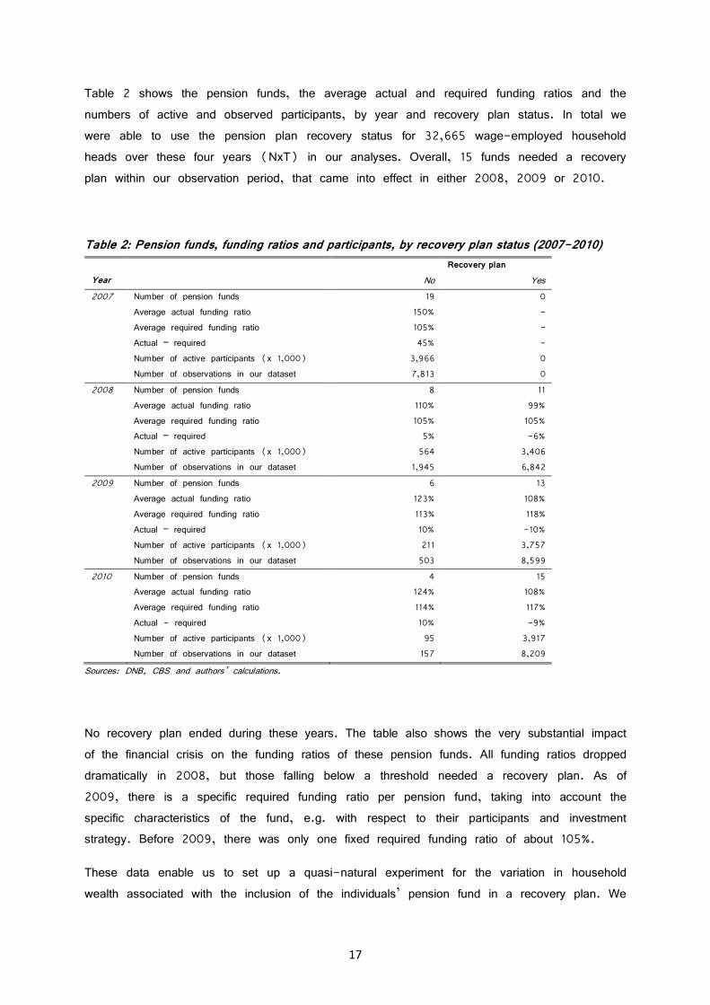
Table 2 shows the pension funds, the average actual and required funding ratios and the

numbers of active and observed participants, by year and recovery plan status. In total we

were able to use the pension plan recovery status for 32,665 wage-employed household

heads over these four years (NxT) in our analyses. Overall, 15 funds needed a recovery

plan within our observation period, that came into effect in either 2008, 2009 or 2010.

Table 2: Pension funds, funding ratios and participants, by recovery plan status (2007-2010)

Recovery plan

Year No Yes

2007 Number of pension funds 19 0

Average actual funding ratio 150% -

Average required funding ratio 105% -

Actual – required 45% -

Number of active participants (x 1,000) 3,966 0

Number of observations in our dataset 7,813 0

2008 Number of pension funds 8 11

Average actual funding ratio 110% 99%

Average required funding ratio 105% 105%

Actual – required 5% -6%

Number of active participants (x 1,000) 564 3,406

Number of observations in our dataset 1,945 6,842

2009 Number of pension funds 6 13

Average actual funding ratio 123% 108%

Average required funding ratio 113% 118%

Actual – required 10% -10%

Number of active participants (x 1,000) 211 3,757

Number of observations in our dataset 503 8,599

2010 Number of pension funds 4 15

Average actual funding ratio 124% 108%

Average required funding ratio 114% 117%

Actual - required 10% -9%

Number of active participants (x 1,000) 95 3,917

Number of observations in our dataset 157 8,209

Sources: DNB, CBS and authors’ calculations.

No recovery plan ended during these years. The table also shows the very substantial impact

of the financial crisis on the funding ratios of these pension funds. All funding ratios dropped

dramatically in 2008, but those falling below a threshold needed a recovery plan. As of

2009, there is a specific required funding ratio per pension fund, taking into account the

specific characteristics of the fund, e.g. with respect to their participants and investment

strategy. Before 2009, there was only one fixed required funding ratio of about 105%.

These data enable us to set up a quasi-natural experiment for the variation in household

wealth associated with the inclusion of the individuals’ pension fund in a recovery plan. We

18

use a diff in diff approach where those subject to underfunding (indicated by the implementation

of a recovery plan) are the treated group, while those with a financially healthier pension

fund, are the control group. We therefore estimate:

9:;� =45 + 4�A;���BC�DBE� + 4%A;�FBEG;HE#IEJ + 46A�+BC� +=;�> ?@ + 8;� (6)

Where the (interaction) dummy A;���BC�DBE� is 1 if individual i’s pension fund carries out a recovery plan in year t and beyond, and 0 otherwise.17 A;�FBEG;HE#IEJ contains a complete

set of pension fund dummies, indicating in which fund the individual K participates. A�+BC� is a set of year dummies and =;�> is a vector of control variables, including (an approximation

of) permanent income and its variance. In this equation 4� represents the causal effect of having a pension fund with a recovery plan on household wealth accumulation that can be

identified by the difference over time and across treated groups.

6 Empirical results

In this section we will present the results of our empirical analyses. First, we will take a

look at our quasi-experiment. Second, we will show several estimation results of the

displacement effect, separately for the wage-employed and for the self-employed, using

several estimation techniques. Here, we begin with standard OLS regression estimates and

consecutively explore Instrumental Variable (IV) analysis and Propensity Score Matching

(PSM) to further specify and sharpen the results.

6.1 Difference-in-differences

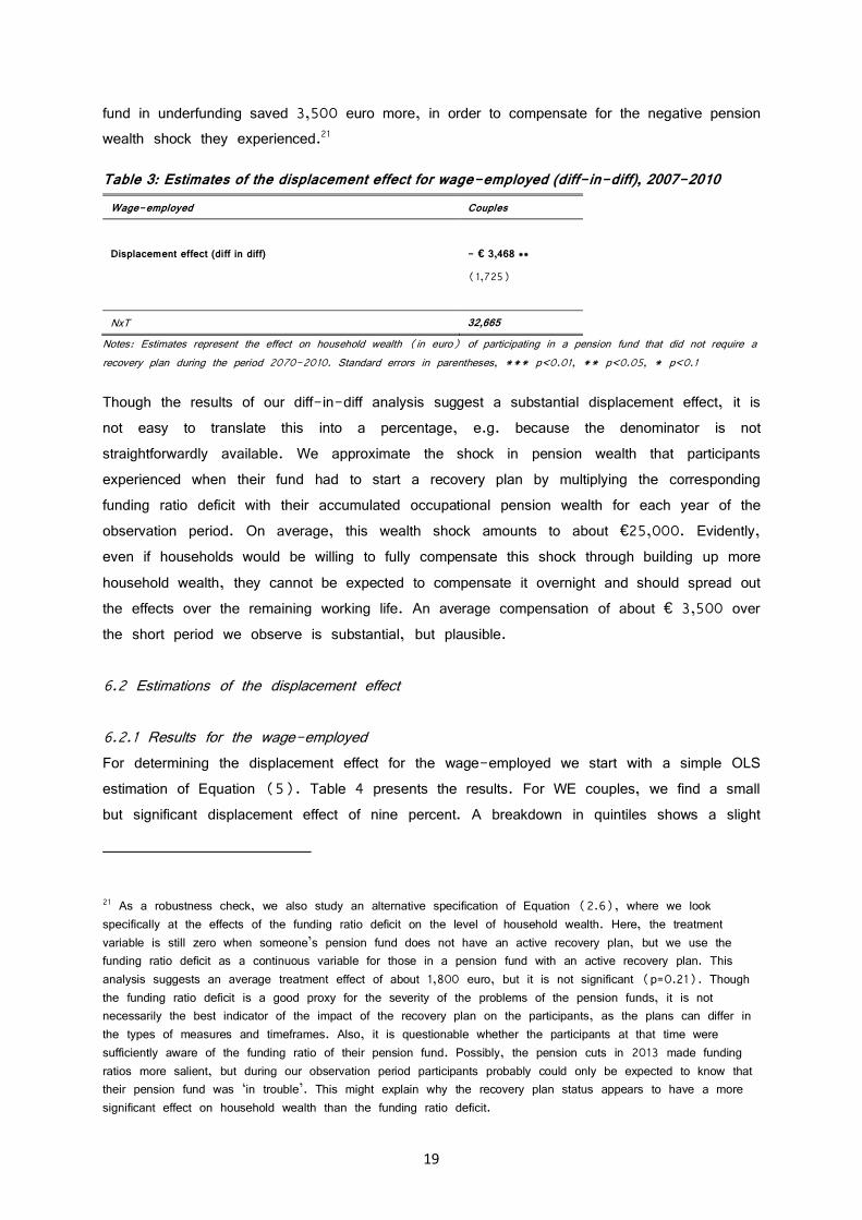
We use a fixed effect (FE) model for the estimation of Equation (6).18 Table 3 shows

the displacement effect of the wage-employed couples who participate in a pension fund that

did not require a recovery plan, compared to participating in a pension fund that did require

a recovery plan.19,20 Full regression results can be found in Table 10 in Appendix 4. Those

with a pension fund with no underfunding accumulated on average 3,500 euro less household

wealth over the period 2007-2010. Alternatively, one could state that those with a pension

17 No recovery plan started before 2008 and none ended within the observation period 2007-2010. 18 We also performed a random effect regression analysis. Results were comparable, with an estimated

displacement effect of -€ 3,993 (p<0.05), but based on the Hausman test we prefer the FE estimate. 19 In this case we present the results for the control group, whose pension fund did not need a recovery plan,

because that is more in line with the other displacement effects in our paper. 20 We also performed this analysis for wage-employed singles, but these results were not significant, possibly

due to the substantially lower number of available observations.

19

fund in underfunding saved 3,500 euro more, in order to compensate for the negative pension

wealth shock they experienced.21

Table 3: Estimates of the displacement effect for wage-employed (diff-in-diff), 2007-2010

Wage-employed Couples

Displacement effect (diff in diff) - € 3,468 **

(1,725)

NxT 32,665

Notes: Estimates represent the effect on household wealth (in euro) of participating in a pension fund that did not require a

recovery plan during the period 2070-2010. Standard errors in parentheses, *** p<0.01, ** p<0.05, * p<0.1

Though the results of our diff-in-diff analysis suggest a substantial displacement effect, it is

not easy to translate this into a percentage, e.g. because the denominator is not

straightforwardly available. We approximate the shock in pension wealth that participants

experienced when their fund had to start a recovery plan by multiplying the corresponding

funding ratio deficit with their accumulated occupational pension wealth for each year of the

observation period. On average, this wealth shock amounts to about €25,000. Evidently,

even if households would be willing to fully compensate this shock through building up more

household wealth, they cannot be expected to compensate it overnight and should spread out

the effects over the remaining working life. An average compensation of about € 3,500 over

the short period we observe is substantial, but plausible.

6.2 Estimations of the displacement effect

6.2.1 Results for the wage-employed

For determining the displacement effect for the wage-employed we start with a simple OLS

estimation of Equation (5). Table 4 presents the results. For WE couples, we find a small

but significant displacement effect of nine percent. A breakdown in quintiles shows a slight

21 As a robustness check, we also study an alternative specification of Equation (2.6), where we look

specifically at the effects of the funding ratio deficit on the level of household wealth. Here, the treatment

variable is still zero when someone’s pension fund does not have an active recovery plan, but we use the

funding ratio deficit as a continuous variable for those in a pension fund with an active recovery plan. This

analysis suggests an average treatment effect of about 1,800 euro, but it is not significant (p=0.21). Though

the funding ratio deficit is a good proxy for the severity of the problems of the pension funds, it is not

necessarily the best indicator of the impact of the recovery plan on the participants, as the plans can differ in

the types of measures and timeframes. Also, it is questionable whether the participants at that time were

sufficiently aware of the funding ratio of their pension fund. Possibly, the pension cuts in 2013 made funding

ratios more salient, but during our observation period participants probably could only be expected to know that

their pension fund was ‘in trouble’. This might explain why the recovery plan status appears to have a more

significant effect on household wealth than the funding ratio deficit.

20

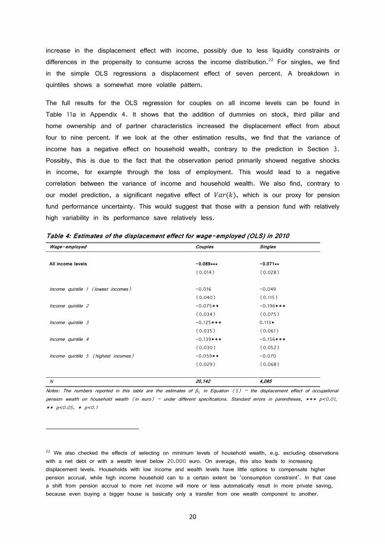
increase in the displacement effect with income, possibly due to less liquidity constraints or

differences in the propensity to consume across the income distribution.22 For singles, we find

in the simple OLS regressions a displacement effect of seven percent. A breakdown in

quintiles shows a somewhat more volatile pattern.

The full results for the OLS regression for couples on all income levels can be found in

Table 11a in Appendix 4. It shows that the addition of dummies on stock, third pillar and

home ownership and of partner characteristics increased the displacement effect from about

four to nine percent. If we look at the other estimation results, we find that the variance of

income has a negative effect on household wealth, contrary to the prediction in Section 3.

Possibly, this is due to the fact that the observation period primarily showed negative shocks

in income, for example through the loss of employment. This would lead to a negative

correlation between the variance of income and household wealth. We also find, contrary to

our model prediction, a significant negative effect of LM��$�, which is our proxy for pension fund performance uncertainty. This would suggest that those with a pension fund with relatively

high variability in its performance save relatively less.

Table 4: Estimates of the displacement effect for wage-employed (OLS) in 2010

Wage-employed Couples Singles

All income levels -0.089*** -0.071**

(0.014) (0.028)

Income quintile 1 (lowest incomes) -0.016 -0.049

(0.040) (0.115)

Income quintile 2 -0.075** -0.196***

(0.034) (0.075)

Income quintile 3 -0.125*** 0.113*

(0.035) (0.061)

Income quintile 4 -0.139*** -0.156***

(0.030) (0.052)

Income quintile 5 (highest incomes) -0.059** -0.070

(0.029) (0.068)

N 20,142 4,085

Notes: The numbers reported in this table are the estimates of 4� in Equation (5) – the displacement effect of occupational

pension wealth on household wealth (in euro) – under different specifications. Standard errors in parentheses, *** p<0.01,

** p<0.05, * p<0.1

22 We also checked the effects of selecting on minimum levels of household wealth, e.g. excluding observations

with a net debt or with a wealth level below 20.000 euro. On average, this also leads to increasing

displacement levels. Households with low income and wealth levels have little options to compensate higher

pension accrual, while high income household can to a certain extent be ‘consumption constraint’. In that case

a shift from pension accrual to more net income will more or less automatically result in more private saving,

because even buying a bigger house is basically only a transfer from one wealth component to another.

21

Instrumental Variable (IV) analysis

The OLS regressions showed significant, but very small displacement effects. As discussed

before, we expect these results to be biased downwards, due to remaining unobserved

heterogeneity and possible measurement errors. That is why next we will apply instrumental

variable analyses to further determine the displacement effect for wage–employed. We discussed

before that pension scheme participation is strongly correlated with company size and sector.

This qualifies them as potentially suitable instruments for the relationship between pension

wealth and household wealth. For company size, we use the log of the number of employees

in the company where the wage-employed works.23 For sector we use the 13 dummies as

shown in Table 9c. The first stage regression results, which can be found in Appendix 4,

Table 11b, confirm that these instruments are strongly correlated with occupational pension

wealth.24 Yet, they should also be uncorrelated with the error in the second stage of the

regression model and the Sargan test for overidentifying restrictions suggests that not all of

our IV’s are exogenous. Employees could sort into differently sized companies and into

separate sectors, partly based on (or correlated with) risk and saving preferences. We

acknowledge the potential limitations of our available instruments. They probably cannot fully

correct for the biases in the displacement effect caused by unobserved heterogeneity and

might even cause some biases themselves. However, given the common levels of displacement

found in the literature and the known strong biases in the OLS estimates, we consider the

IV results an improvement.

Table 5 shows the results for the IV analyses for couples. The displacement effect is now

-33%, thus substantially larger, and (strongly) significant.25 This is also true in the case of

the separate income quintiles, where the (significant) displacement effects range between -

21% and -61%. Again, the displacement effect primarily rises with income. For singles the

overall displacement effect in the IV analyses also becomes much stronger, at around -38%.

But the breakup in income quintiles shows mostly non-significant results. The full results of

the IV regression for couples over all income levels are shown in Table 11a in Appendix 4.

23 We use the log of company size since the company size distribution is strongly positively skewed. When we

perform a first stage regression on 6 splines for the log of firm size, we find that the effect of the log of firm

size on accumulated occupational pension wealth is discontinuous, but from the 25th to the 75th percentile it is

smoothly and significantly positive. 24 The F statistic on the joint significance of the instruments in the first stage regression equals 170.6,

indicating that the instruments are relevant. 25 We checked how sensitive this result is to different assumptions for the discount rate we use to calculate

the current level of accumulated pension wealth. This sensitivity turns out to be limited. If, instead of a

discount rate of 1.5%, we use 2,5% (or 0,5%), the displacement effect (IV) would be -36% (or -29%).

If we remove firm size as instrument, the estimate of the displacement effect shrinks from -33% to -32%.

22

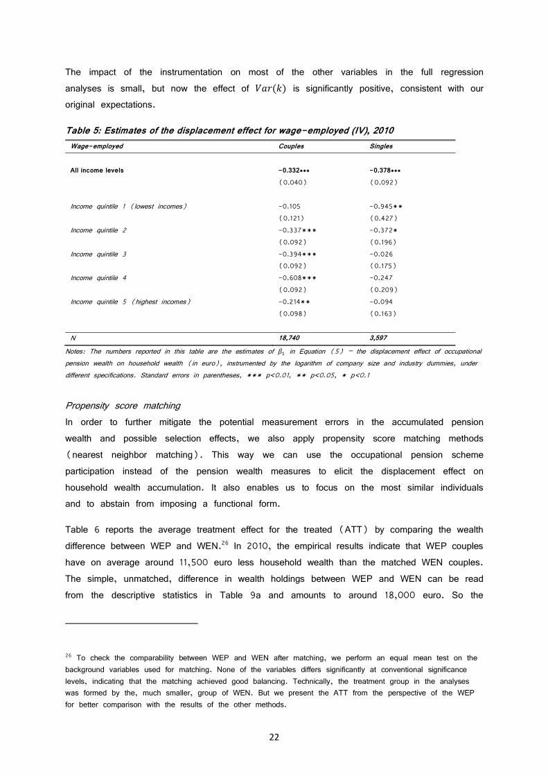
The impact of the instrumentation on most of the other variables in the full regression

analyses is small, but now the effect of LM��$� is significantly positive, consistent with our original expectations.

Table 5: Estimates of the displacement effect for wage-employed (IV), 2010

Wage-employed Couples Singles

All income levels -0.332*** -0.378***

(0.040) (0.092)

Income quintile 1 (lowest incomes) -0.105 -0.945**

(0.121) (0.427)

Income quintile 2 -0.337*** -0.372*

(0.092) (0.196)

Income quintile 3 -0.394*** -0.026

(0.092) (0.175)

Income quintile 4 -0.608*** -0.247

(0.092) (0.209)

Income quintile 5 (highest incomes) -0.214** -0.094

(0.098) (0.163)

N 18,740 3,597

Notes: The numbers reported in this table are the estimates of 4� in Equation (5) – the displacement effect of occupational

pension wealth on household wealth (in euro), instrumented by the logarithm of company size and industry dummies, under

different specifications. Standard errors in parentheses, *** p<0.01, ** p<0.05, * p<0.1

Propensity score matching

In order to further mitigate the potential measurement errors in the accumulated pension

wealth and possible selection effects, we also apply propensity score matching methods

(nearest neighbor matching). This way we can use the occupational pension scheme

participation instead of the pension wealth measures to elicit the displacement effect on

household wealth accumulation. It also enables us to focus on the most similar individuals

and to abstain from imposing a functional form.

Table 6 reports the average treatment effect for the treated (ATT) by comparing the wealth

difference between WEP and WEN.26 In 2010, the empirical results indicate that WEP couples

have on average around 11,500 euro less household wealth than the matched WEN couples.

The simple, unmatched, difference in wealth holdings between WEP and WEN can be read

from the descriptive statistics in Table 9a and amounts to around 18,000 euro. So the

26 To check the comparability between WEP and WEN after matching, we perform an equal mean test on the

background variables used for matching. None of the variables differs significantly at conventional significance

levels, indicating that the matching achieved good balancing. Technically, the treatment group in the analyses

was formed by the, much smaller, group of WEN. But we present the ATT from the perspective of the WEP

for better comparison with the results of the other methods.

23

matching results suggest that this simple difference would be an overestimation of the true

displacement effect. In Table 6, we also tentatively compare these numbers with the average

difference in occupational pension wealth between the two groups. This way, we include the

potentially flawed pension wealth data in this robustness analysis after all, but it gives us an

idea of the magnitude of the displacement effect. The matched difference in occupational

pension wealth is slightly smaller than the unmatched descriptive statistics suggest. Together,

these two matched amounts suggest the displacement effect is about -24% for couples. For

the matched single households, the difference in household wealth is just over 21,000 euro

and the difference in occupation pension wealth is about 26,500 euro, suggesting a

displacement effect of -80%.

Table 6: Estimates of the displacement effect for wage-employed (PSM), 2010

Wage-employed Couples Singles

ATT – Matched difference in household wealth - € 11,430 * - € 21,203 ***

(i.e. the HW of WEP minus the HW of WEN) (7,177) (9,537)

Matched difference in HH occupational pension wealth € 47,793 *** € 26,506 ***

(3,161) (4,592)

Tentative displacement effect of PW on HW - 24% - 80%

N 18,740 3,597

Notes: Standard errors in parentheses, *** p<0.01, ** p<0.05, * p<0.1

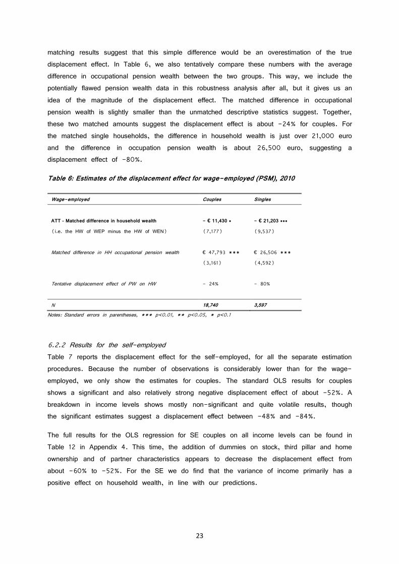
6.2.2 Results for the self-employed

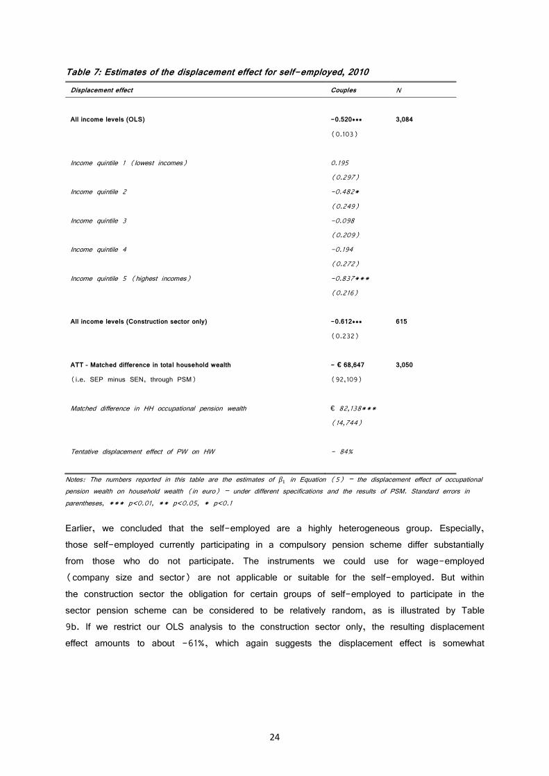
Table 7 reports the displacement effect for the self-employed, for all the separate estimation

procedures. Because the number of observations is considerably lower than for the wage-

employed, we only show the estimates for couples. The standard OLS results for couples

shows a significant and also relatively strong negative displacement effect of about -52%. A

breakdown in income levels shows mostly non-significant and quite volatile results, though

the significant estimates suggest a displacement effect between -48% and -84%.

The full results for the OLS regression for SE couples on all income levels can be found in

Table 12 in Appendix 4. This time, the addition of dummies on stock, third pillar and home

ownership and of partner characteristics appears to decrease the displacement effect from

about -60% to -52%. For the SE we do find that the variance of income primarily has a

positive effect on household wealth, in line with our predictions.

24

Table 7: Estimates of the displacement effect for self-employed, 2010

Displacement effect Couples N

All income levels (OLS) -0.520*** 3,084

(0.103)

Income quintile 1 (lowest incomes) 0.195

(0.297)

Income quintile 2 -0.482*

(0.249)

Income quintile 3 -0.098

(0.209)

Income quintile 4 -0.194

(0.272)

Income quintile 5 (highest incomes) -0.837***

(0.216)

All income levels (Construction sector only) -0.612*** 615

(0.232)

ATT – Matched difference in total household wealth - € 68,647 3,050

(i.e. SEP minus SEN, through PSM) (92,109)

Matched difference in HH occupational pension wealth € 82,138***

(14,744)

Tentative displacement effect of PW on HW - 84%

Notes: The numbers reported in this table are the estimates of 4� in Equation (5) – the displacement effect of occupational

pension wealth on household wealth (in euro) – under different specifications and the results of PSM. Standard errors in

parentheses, *** p<0.01, ** p<0.05, * p<0.1

Earlier, we concluded that the self-employed are a highly heterogeneous group. Especially,

those self-employed currently participating in a compulsory pension scheme differ substantially

from those who do not participate. The instruments we could use for wage-employed

(company size and sector) are not applicable or suitable for the self-employed. But within

the construction sector the obligation for certain groups of self-employed to participate in the

sector pension scheme can be considered to be relatively random, as is illustrated by Table

9b. If we restrict our OLS analysis to the construction sector only, the resulting displacement

effect amounts to about -61%, which again suggests the displacement effect is somewhat

25

stronger for the self-employed than for the wage-employed.27 The full regression results can

be found in Table 12.

When we apply propensity score matching, to circumvent the measurement errors in the

pension wealth measures and to select the most similar individuals, we find that the matched

self-employed couples have accumulated around 69,000 euro less household wealth if they

are affiliated to the occupational pension system, but this estimate is not significant. Compared

to the matched difference in occupational pension wealth the tentative displacement effect

would be around -84%.

7 Conclusion

We look at the displacement effect from mandatory occupational pension saving on household

wealth in the Netherlands, taking institutional differences among occupations into account.

Where most wage-employed in the Netherlands participate in a mandatory occupational pension

scheme, a substantial minority of about 9% – known in the Netherlands as the white spot

(”witte vlek”) – does not participate. Conversely, while most self-employed are fully

responsible for their own pension accrual (on top of the state pension), some groups of

self-employed (about 7% in total) are obliged to participate in a professional or industry

pension fund. This allows us to separately measure the displacement effects within these

groups, thus controlling for unobserved characteristics that correlate with the occupational

choice between working as wage-employed or self-employed.

For the wage employed couples we first perform a difference-in-differences analysis, based

on a quasi-natural experiment. We use the differential impact of the financial crisis on the

separate pension funds in the Netherlands, and find that those whose pension fund did not

need to apply a recovery plan accumulated about 3,500 euro less household wealth over de

period 2007-2010. This indicates the existence of substantial displacement effects. Standard

OLS regression results suggest only limited displacement effects for wage-employed couples,

but based on IV analyses our estimate rises to about –33%. Further analyses on separate

income quintiles suggest the displacement effects rise with income, with estimates for the

higher income levels up to -61%. Propensity score matching analyses also point at a fairly

27 A Chow test, based on an identical OLS regression specification for both groups, indicates that the

displacement effect is significantly higher for self-employed than for wage-employed (F-statistics 821.70,

p<0.001). This is also the case when we focus only on those self-employed in construction (F-statistics

63.35, p<0.001). However, the confidence interval for the displacement effect of self-employed does include

the IV estimate of the wage-employed (not vice versa), which calls for some caution in interpreting the

differences between them. We hypothesize that higher awareness of pension rights accumulation and lower risk-

aversion could lead to higher displacement effects for self-employed. To the (limited) extent that we can proxy

for this in our data, our checks suggest that awareness is the more important factor in explaining the difference

between self-employed and wage-employed.

26

substantial displacement effects, with an average treatment effect for the treated of 11,500

euro (suggesting a displacement effect of about -24%).

For the self-employed we already find a quite strong displacement effect in our standard

OLS analyses of about -52%. An analysis on only the construction sector, where compulsory

pension scheme participation by the self-employed is arguably more random than in other

sectors, raises this estimate to about -61%. Propensity score matching also shows a very

substantial displacement effect of about 69,000 euro (or about -80%), but this could only

be estimated very imprecisely.

Overall, our results suggest a larger displacement effect for self-employed than for wage-

employed. One possible explanation lies in the fact that self-employed can on average be

expected to be much more aware of the pension entitlements they do or do not accrue than

wage-employed, especially those wage-employed in the white spot. Such a higher awareness

would lead to an on average higher displacement effect among self-employed than among

wage-employed (Card and Ransom, 2011; Bottazzi et al., 2006). Another potential

explanation is that self-employed are on average less risk-averse than wage-employed and

thus, ceteris paribus, would hold less precautionary savings.

Acknowledgments

The authors would like to thank Hans Bloemen, Stefan Hochguertel, Dario Sansone, Marike

Knoef, Peter Kooreman, Jan Potters, Nicole Bosch and Gijs Roelofs, and Eduard Suari-Andreu and the other participants of the Netspar Pension Day on October 1, 2015 in Utrecht

for valuable comments and suggestions.

27

Bibliography

Alessie, R., Angelini, V., & Van Santen, P. (2013). Pension wealth and household savings in

Europe: Evidence from SHARELIFE. European Economic Review, 63, 308-328.

Alessie, R. J., Kapteyn, A., & Klijn, F. (1997). Mandatory Pensions and Personal Savings in

The Netherlands*. De Economist, 145(3), 291-324. Attanasio, O. and A. Brugiavini (2003):

“Social Sec

urity and Households’ Saving”, The Quarterly Journal of Economics, 118:3, pp. 1075-1119.

Attanasio, O. P., & Rohwedder, S. (2003). Pension wealth and household saving: Evidence from

pension reforms in the United Kingdom. American Economic Review,1499-1521.

Bottazzi, R., Jappelli, T., & Padula, M. (2006). Retirement expectations, pension reforms, and

their impact on private wealth accumulation. Journal of Public Economics, 90(12), 2187-2212.

Card, D., & Ransom, M. (2011). Pension plan characteristics and framing effects in employee

savings behavior. The Review of Economics and Statistics, 93(1),228-243.

Disney, R. (2006). Household Saving Rates and the Design of Public Pension Programmes:

Cross–Country Evidence. National Institute Economic Review, 198(1), 61-74.

Engelhardt, G. V., & Kumar, A. (2011). Pensions and household wealth accumulation. Journal of

Human Resources, 46(1), 203-236.

Euwals, R. (2000). Do mandatory pensions decrease household savings? Evidence for the

Netherlands.

De Economist, 148(5), 643-670.

Feldstein, M. (1974): “Social Security, Induced Retirement and Aggregate Capital Accumulation”,

Journal of Political Economy, 82:5, pp. 905-926.

Gale, W. (1995). The Effects of Pensions on Wealth: A Re-evaluation of Theory and Evidence.

Manuscript.Washington: Brookings Inst., 1995. 27

Gale, W. (1998). The Effects of Pensions on Household Wealth: A Reevaluation of Theory and

Evidence, Journal of Political Economy, 106:4, pp. 706-722.

Gruber, J., & Wise, D. (1999). Social security programs and retirement around the world.

Research in Labor Economics, 18(1),40.

Gruber, J., & Wise, D. A. (Eds.). (2008). Social security and retirement around the world.

University of Chicago Press.

28

Hartog, J., Ferrer-i-Carbonell, A., & Jonker, N. (2002). Linking measured risk aversion to

individual characteristics. Kyklos,55(1), 3-26.

Hurd, M., Michaud, P. C., & Rohwedder, S. (2012). The displacement effect of public pensions

on the accumulation of financial assets. Fiscal studies, 33(1), 107-128.

Kapteyn A., Alessie R., Lusardi A.(2005),Explaining the wealth holdings of different cohorts:

productivity growth and Social Security, European Economic Review 49 (2005) 1361 – 1391.

Kapteyn, A. and S. Panis (2005): “Institutions and Saving for Retirement: Comparing the United

States, Italy, and The Netherlands”, in D.A. Wise (ed.) Analyses in the Economics of Aging,

University of Chicago Press, pp.281-312.

Kotlikoff, L. (1979): “Testing the Theory of Social Security and Life Cycle Accumulation”, American

Economic Review , 69:3, pp. 396-410.

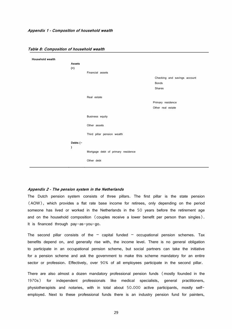
29

Appendix 1 – Composition of household wealth

Table 8: Composition of household wealth

Household wealth

Assets

(+)

Financial assets

Checking and savings account

Bonds

Shares

Real estate

Primary residence

Other real estate

Business equity

Other assets

Third pillar pension wealth

Debts (-

)

Mortgage debt of primary residence

Other debt

Appendix 2 – The pension system in the Netherlands

The Dutch pension system consists of three pillars. The first pillar is the state pension

(AOW), which provides a flat rate base income for retirees, only depending on the period

someone has lived or worked in the Netherlands in the 50 years before the retirement age

and on the household composition (couples receive a lower benefit per person than singles).

It is financed through pay-as-you-go.

The second pillar consists of the – capital funded – occupational pension schemes. Tax

benefits depend on, and generally rise with, the income level. There is no general obligation

to participate in an occupational pension scheme, but social partners can take the initiative

for a pension scheme and ask the government to make this scheme mandatory for an entire

sector or profession. Effectively, over 90% of all employees participate in the second pillar.

There are also almost a dozen mandatory professional pension funds (mostly founded in the

1970s) for independent professionals like medical specialists, general practitioners,

physiotherapists and notaries, with in total about 50.000 active participants, mostly self-

employed. Next to these professional funds there is an industry pension fund for painters,

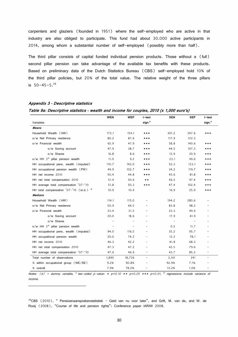
30

carpenters and glaziers (founded in 1951) where the self-employed who are active in that

industry are also obliged to participate. This fund had about 30.000 active participants in

2014, among whom a substantial number of self-employed (possibly more than half).

The third pillar consists of capital funded individual pension products. Those without a (full)

second pillar pension can take advantage of the available tax benefits with these products.

Based on preliminary data of the Dutch Statistics Bureau (CBS) self-employed hold 10% of

the third pillar policies, but 20% of the total value. The relative weight of the three pillars

is 50-45-5.28

Appendix 3 – Descriptive statistics

Table 9a: Descriptive statistics – wealth and income for couples, 2010 (x 1,000 euro’s)

Variables

WEN

WEP

t-test

sign.A

SEN

SEP

t-test

sign.A

Means

Household Wealth (HW) 172.1 154.1 *** 301.2 397.6 ***

o/w Net Primary residence 80.2 87.6 *** 117.9 122.3

o/w Financial wealth 65.9 47.9 *** 58.8 140.6 ***

o/w Saving account 47.9 38.7 *** 44.5 107.3 ***

o/w Shares 16.8 8.6 *** 12.9 30.9 ***

o/w HH 3rd pillar pension wealth 11.0 9.2 *** 23.1 49.6 ***

HH occupational pens. wealth (imputed) 110.7 142.0 *** 52.3 133.1 ***

HH occupational pension wealth (PW) 49.9 102.7 *** 34.2 119.7 ***

HH net income 2010 50.4 44.8 *** 45.6 81.8 ***

HH net total compensation 2010 51.4 50.6 ** 46.5 97.4 ***

HH average total compensation ’07-‘10 51.8 50.3 *** 47.4 102.4 ***

HH total compensation ’07-’10 (st.d.) B 10.9 10.4 16.9 25.9 ***

Medians

Household Wealth (HW) 114.1 115.0 - 194.2 280.6 -

o/w Net Primary residence 50.9 64.5 - 83.8 98.2 -

o/w Financial wealth 23.9 21.5 - 22.3 49.9 -

o/w Saving account 20.0 18.6 - 17.9 41.9 -

o/w Shares - - - - - -

o/w HH 3rd pillar pension wealth - - - 0.5 11.7 -

HH occupational pens. wealth (imputed) 94.0 116.5 - 35.2 95.7 -

HH occupational pension wealth 20.0 74.2 - 12.2 78.1 -

HH net income 2010 46.3 42.2 - 41.8 68.3 -

HH net total compensation 2010 47.3 47.2 - 42.5 79.6 -

HH average total compensation ’07-‘10 47.6 46.9 - 43.7 85.2 -

Total number of observations 1,890 18,726 - 3,161 241 -

% within occupational group (WE/SE) 9.2% 90.8% - 92.9% 7.1% -

% overall 7.9% 78.0% - 13.2% 1.0% -

Notes: (d) = dummy variable, A two-sided p-value: * p<0.10 ** p<0.05 *** p<0.01, B regressions include variance of

income.

28CBS (2010), “ Pensioenaansprakenstatistiek - Geld van nu voor later”, and Grift, M. van de, and W. de

Rooij (2008), “Course of life and pension rights”: Conference paper IARIW 2008.

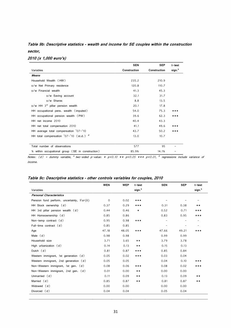
31

Table 9b: Descriptive statistics – wealth and income for SE couples within the construction

sector,

2010 (x 1,000 euro’s)

Variables

SEN

Construction

SEP

Construction

t-test

sign.A

Means

Household Wealth (HW) 235.2 210.9

o/w Net Primary residence 120.8 110.7

o/w Financial wealth 41.3 45.3

o/w Saving account 32.1 31.7

o/w Shares 8.8 13.5

o/w HH 3rd pillar pension wealth 20.1 17.8

HH occupational pens. wealth (imputed) 54.0 75.3 ***

HH occupational pension wealth (PW) 39.6 62.3 ***

HH net income 2010 40.4 43.3

HH net total compensation 2010 41.1 49.6 ***

HH average total compensation ’07-‘10 43.7 50.2 ***

HH total compensation ’07-’10 (st.d.) B 13.0 10.7

Total number of observations 577 95 -

% within occupational group (SE in construction) 85.9% 14.1% -

Notes: (d) = dummy variable, A two-sided p-value: * p<0.10 ** p<0.05 *** p<0.01, B regressions include variance of

income.

Table 9c: Descriptive statistics – other controls variables for couples, 2010

Variables

WEN

WEP

t-test

sign.A

SEN

SEP

t-test

sign.A

Personal Characteristics

Pension fund perform. uncertainty, LM��$� 0 0.02 *** - - -

HH Stock ownership (d) 0.37 0.29 *** 0.31 0.38 **

HH 3rd pillar pension wealth (d) 0.44 0.46 * 0.52 0.71 ***

HH Homeownership (d) 0.85 0.86 0.83 0.95 ***

Non-temp contract (d) 0.95 0.98 *** - - -

Full-time contract (d) 0.85 0.85 - - -

Age 47.18 48.05 *** 47.66 49.21 ***

Male (d) 0.98 0.98 0.99 0.99

Household size 3.71 3.65 ** 3.79 3.78

High urbanization (d) 0.14 0.13 ** 0.15 0.13

Dutch (d) 0.81 0.87 *** 0.85 0.84

Western immigrant, 1st generation (d) 0.05 0.02 *** 0.03 0.04

Western immigrant, 2nd generation (d) 0.05 0.05 0.04 0.10 ***

Non-Western immigrant, 1st gen. (d) 0.08 0.06 *** 0.08 0.02 ***

Non-Western immigrant, 2nd gen. (d) 0.01 0.00 ** 0.00 0.00

Unmarried (d) 0.11 0.09 ** 0.13 0.09 **

Married (d) 0.85 0.87 ** 0.81 0.87 **

Widowed (d) 0.00 0.00 0.00 0.00

Divorced (d) 0.04 0.04 0.05 0.04

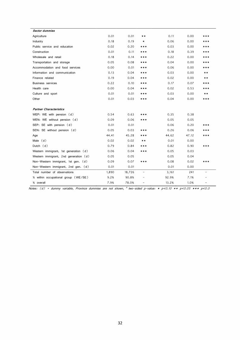
32

Sector dummies

Agriculture 0.01 0.01 ** 0.11 0.00 ***

Industry 0.18 0.19 * 0.06 0.00 ***

Public service and education 0.02 0.20 *** 0.03 0.00 ***

Construction 0.01 0.11 *** 0.18 0.39 ***

Wholesale and retail 0.18 0.14 *** 0.22 0.00 ***

Transportation and storage 0.05 0.08 *** 0.04 0.00 ***

Accommodation and food services 0.00 0.01 *** 0.06 0.00 ***

Information and communication 0.13 0.04 *** 0.03 0.00 **

Finance related 0.19 0.04 *** 0.02 0.00 **

Business services 0.22 0.10 *** 0.17 0.07 ***

Health care 0.00 0.04 *** 0.02 0.53 ***

Culture and sport 0.01 0.01 *** 0.03 0.00 **

Other 0.01 0.03 *** 0.04 0.00 ***

Partner Characteristics

WEP: WE with pension (d) 0.54 0.63 *** 0.35 0.38

WEN: WE without pension (d) 0.09 0.06 *** 0.05 0.05

SEP: SE with pension (d) 0.01 0.01 0.06 0.20 ***

SEN: SE without pension (d) 0.05 0.03 *** 0.26 0.06 ***

Age 44.41 45.28 *** 44.62 47.12 ***

Male (d) 0.02 0.02 ** 0.01 0.00

Dutch (d) 0.79 0.84 *** 0.82 0.90 ***

Western immigrant, 1st generation (d) 0.06 0.04 *** 0.05 0.03

Western immigrant, 2nd generation (d) 0.05 0.05 0.05 0.04

Non-Western immigrant, 1st gen. (d) 0.09 0.07 *** 0.08 0.02 ***

Non-Western immigrant, 2nd gen. (d) 0.01 0.01 0.01 0.00

Total number of observations 1,890 18,726 - 3,161 241 -

% within occupational group (WE/SE) 9.2% 90.8% - 92.9% 7.1% -

% overall 7.9% 78.0% - 13.2% 1.0% -

Notes: (d) = dummy variable, Province dummies are not shown, A two-sided p-value: * p<0.10 ** p<0.05 *** p<0.0

33

Appendix 4 – Full regression results

Table 10: full results FE GLS difference-in-differences analyses, 2007-2010

Household Wealth (HW) WE-couples

Treatment (dummy recovery plan) 3468**

(1725)

HH average total compensation ’07-‘10 -0.665

(1.052)

HH variance total compensation ’07-‘10 -0.000

(0.000)

Age 3.57 x 104

(2.98 x 104)

Age2 -940

(598)

Age3 7.02

(4.01)

Household size 4284***

(1605)

High urbanization (d) 6962

(5501)

Married (d) 7695

(8922)

Widowed (d) 48252

(42107)

Divorced (d) 39170

(12284)

Stock ownership (d) 3034

(2382)

3rd pillar pension wealth ownership (d) 9207

(7915)

Homeownership (d) 1.32 x 105***

(4660)

Non-temp contract (d) -1.42 x 104

(1.22 x 104)

Full-time contract (d) 162

(1711)

Partner is WE with pension (d) -3533*

(2066)

Partner is WE without pension (d) -1158

(3221)

Partner is SE with pension (d) -1462

(7856)

Partner is SE without pension (d) 10590

(6440)

Year dummies Yes

Pension fund dummies Yes

Other controls Yes

Constant -1.51 x 106

(9.28 x 105)

R-sqr (within) 0.0835

NxT 32,665

Notes: The numbers reported in this table are the regression estimates of Equation (6), with household wealth (in euro)

as the dependent variable. A complete list of the included partner characteristics can be found in Table 9c.Standard errors in parentheses, *** p<0.01, ** p<0.05, * p<0.1

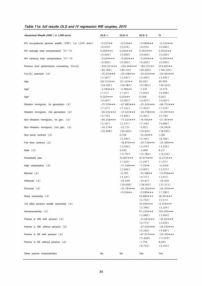
34

Table 11a: full results OLS and IV regression WE couples, 2010

Household Wealth (HW) (in 1,000 euro) OLS-1 OLS-2 OLS-3 IV

HH occupational pension wealth (PW) (in 1,000 euro) -0.037** -0.034** -0.089*** -0.332***

(0.014) (0.014) (0.014) (0.040)

HH average total compensation ’07-‘10 0.004*** 0.004*** 0.003*** 0.003***

(0.000) (0.000) (0.000) (0.000)

HH variance total compensation ’07-‘10 -0.000*** -0.000*** -0.000*** -0.000***

(0.000) (0.000) (0.000) (0.000)

Pension fund performance uncertainty, LM��$� -439.251*** -326.944*** -183.757** 254.825**

(85.189) (89.314) (85.690) (104.520)

LM��$� unknown (d) -35.610*** -29.108*** -25.923*** -20.941***

(3.367) (3.567) (3.420) (3.245)

Age 162.513*** 131.332** 69.053 40.909

(54.595) (54.083) (51.893) (49.022)

Age2 -3.084*** -2.486** -1.235 -0.579

(1.111) (1.101) (1.056) (0.998)

Age3 0.020*** 0.016** 0.008 0.003

(0.007) (0.007) (0.007) (0.007)

Western immigrant, 1st generation (d) -72.109*** -67.885*** -35.343*** -44.703***

(7.371) (7.333) (7.450) (7.219)

Western immigrant, 2nd generation (d) -40.202*** -37.622*** -30.758*** -31.097***

(5.714) (5.665) (5.441) (5.118)

Non-Western immigrant, 1st gen. (d) -84.358*** -77.625*** -14.495** -21.181***

(5.167) (5.331) (7.318) (6.886)

Non-Western immigrant, 2nd gen. (d) -34.374* -23.731 -5.873 -34.042*

(20.808) (20.626) (19.810) (18.494)

Non-temp contract (d) 0.158 -10.264** 1.260

(5.340) (5.144) (8.106)

Full-time contract (d) -18.876*** -20.736*** -25.189***

(3.560) (3.419) (3.226)

Male (d) 4.492 -3.800 8.311

(11.791) (13.786) (13.226)

Household size 10.897*** 10.675*** 12.273***

(1.322) (1.297) (1.211)

High urbanization (d) -17.769*** -7.054* -6.915*

(3.962) (3.819) (3.573)

Married (d) -6.783 -10.188** -13.058***

(4.341) (4.177) (3.911)

Widowed (d) -25.949 -24.877 -24.059

(39.658) (38.005) (37.273)

Divorced (d) -33.781*** -24.302*** -26.361***

-0.034** -0.089*** (7.280)

Stock ownership (d) 59.880*** 58.951***

(2.702) (2.511)

3rd pillar pension wealth ownership (d) 14.590*** 13.914***

(2.396) (2.224)

Homeownership (d) 97.330*** 104.295***

(3.680) (3.600)

Partner is WE with pension (d) -31.063*** -18.691***

(2.773) (2.659)

Partner is WE without pension (d) -27.525*** -24.510***

(5.266) (4.987)

Partner is SE with pension (d) -47.972*** -29.100***

(11.828) (11.079)

Partner is SE without pension (d) -1.754 8.943

(6.742) (6.354)

Other partner characteristics No No Yes Yes

35

Province dummies No No Yes Yes

Constant

-

2916.966***

-

2437.632***

-1561.295*

-1236.499

(887.265) (879.037) (843.182) (795.141)

Adj. R-sqr 0.204 0.220 0.282 0.259

N 20,142 20,142 20,142 18,740

Notes: The numbers reported in this table are the regression estimates of Equation (5) – with household wealth (in 1,000

euro) as the dependent variable – under different specifications. A complete list of the included partner characteristics can be

found in Table 9c. Standard errors in parentheses, *** p<0.01, ** p<0.05, * p<0.1

36

Table 11b: first stage results IV regression WE couples, 2010

HH occupational pension wealth (PW) in 1,000 euro First stage

Sector dummies

Agriculture -72.1***

(6.42)

Industry -43.0***

(3.74)

Public service and education 13.4***

(3.76)

Construction -38.0***

(4.00)

Wholesale and retail -56.7***

(3.88)

Transportation and storage -63.5***

(4.04)

Accommodation and food services -20.1***

(6.64)

Information and communication -55.9***

(4.45)

Finance related -63.1***

(4.26)

Business services -40.1***

(3.96)

Health care 21.2***

(4.64)

Culture and sport -25.3***

(7.08)

Other (reference dummy) .

.

Company size

Log(company size) 2.06***

(0.277)

Other controls Yes

Constant Yes

F-stat 170.6

p-value <0.0001

Notes: The numbers reported in this table are the first stage regression estimates of an IV specification of Equation (5)

with household occupational pension wealth (in 1,000 euro) as the instrumented variable. A complete list of the included controls can be found in Table 11a. Standard errors in parentheses, *** p<0.01, ** p<0.05, * p<0.1

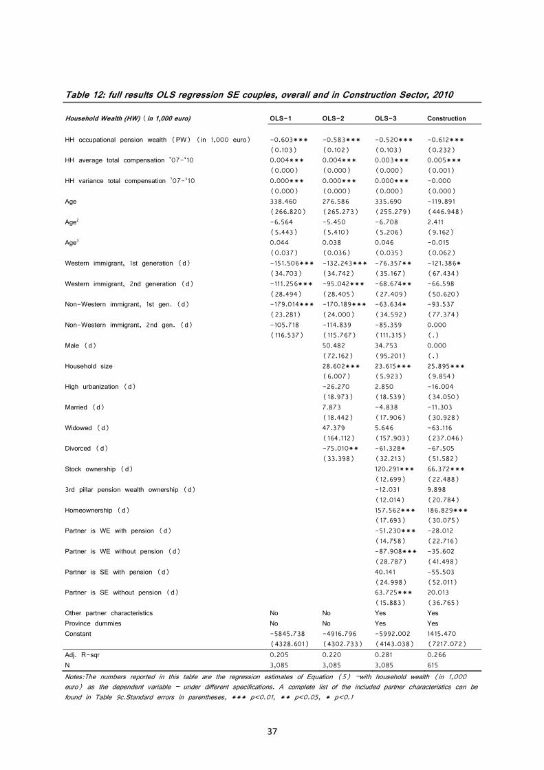
37

Table 12: full results OLS regression SE couples, overall and in Construction Sector, 2010

Household Wealth (HW) (in 1,000 euro) OLS-1 OLS-2 OLS-3 Construction

HH occupational pension wealth (PW) (in 1,000 euro) -0.603*** -0.583*** -0.520*** -0.612***

(0.103) (0.102) (0.103) (0.232)

HH average total compensation ’07-‘10 0.004*** 0.004*** 0.003*** 0.005***

(0.000) (0.000) (0.000) (0.001)

HH variance total compensation ’07-‘10 0.000*** 0.000*** 0.000*** -0.000

(0.000) (0.000) (0.000) (0.000)

Age 338.460 276.586 335.690 -119.891

(266.820) (265.273) (255.279) (446.948)

Age2 -6.564 -5.450 -6.708 2.411

(5.443) (5.410) (5.206) (9.162)

Age3 0.044 0.038 0.046 -0.015

(0.037) (0.036) (0.035) (0.062)

Western immigrant, 1st generation (d) -151.506*** -132.243*** -76.357** -121.386*

(34.703) (34.742) (35.167) (67.434)

Western immigrant, 2nd generation (d) -111.256*** -95.042*** -68.674** -66.598

(28.494) (28.405) (27.409) (50.620)

Non-Western immigrant, 1st gen. (d) -179.014*** -170.189*** -63.634* -93.537

(23.281) (24.000) (34.592) (77.374)

Non-Western immigrant, 2nd gen. (d) -105.718 -114.839 -85.359 0.000

(116.537) (115.767) (111.315) (.)

Male (d) 50.482 34.753 0.000

(72.162) (95.201) (.)

Household size 28.602*** 23.615*** 25.895***

(6.007) (5.923) (9.854)

High urbanization (d) -26.270 2.850 -16.004

(18.973) (18.539) (34.050)

Married (d) 7.873 -4.838 -11.303

(18.442) (17.906) (30.928)

Widowed (d) 47.379 5.646 -63.116

(164.112) (157.903) (237.046)

Divorced (d) -75.010** -61.328* -67.505

(33.398) (32.213) (51.582)

Stock ownership (d) 120.291*** 66.372***

(12.699) (22.488)

3rd pillar pension wealth ownership (d) -12.031 9.898

(12.014) (20.784)

Homeownership (d) 157.562*** 186.829***

(17.693) (30.075)

Partner is WE with pension (d) -51.230*** -28.012

(14.758) (22.716)

Partner is WE without pension (d) -87.908*** -35.602

(28.787) (41.498)

Partner is SE with pension (d) 40.141 -55.503

(24.998) (52.011)

Partner is SE without pension (d) 63.725*** 20.013

(15.883) (36.765)

Other partner characteristics No No Yes Yes

Province dummies No No Yes Yes

Constant -5845.738 -4916.796 -5992.002 1415.470

(4328.601) (4302.733) (4143.038) (7217.072)

Adj. R-sqr 0.205 0.220 0.281 0.266

N 3,085 3,085 3,085 615

Notes:The numbers reported in this table are the regression estimates of Equation (5) –with household wealth (in 1,000 euro) as the dependent variable – under different specifications. A complete list of the included partner characteristics can be

found in Table 9c.Standard errors in parentheses, *** p<0.01, ** p<0.05, * p<0.1