The difference between greenhouse gases and air pollution: TheEnvironmental Kuznets CurveIzaksson, Thomas

CitationIzaksson, T. (2021). The difference between greenhouse gases and air pollution: TheEnvironmental Kuznets Curve. Version: Not Applicable (or Unknown)

License: License to inclusion and publication of a Bachelor or Master thesis inthe Leiden University Student Repository

Downloaded from: https://hdl.handle.net/1887/3239844 Note: To cite this publication please use the final published version (if applicable).

2

Thomas Izaksson | s2038730

Thesis Advisor: Dr. Vrijburg

Date 11-06-2021

Word Count: 15.754

MSc. Public Administration Economics & Governance

Faculty of Governance and Global Affairs

Leiden University

Abstract

The economic concept of an Environmental Kuznets Curve hypothesizes an inverse U-shaped

relationship between environmental quality and economic growth. A better understanding of

the existence of a development path between income and environmental quality can help

provide a baseline scenario and framework for environmental policy. Research on the topic of

the EKC hypothesis is extensive but still mixed and inconclusive. This paper analysis to what

extent and why the effect of economic development on greenhouse gas emissions differs from

the effect of economic development on air pollution. The results show an inverse U-shaped

relationship for PM10. CO2 and SO2 display inverse N-shaped relationships. CH4 displays a

monotonically increasing relationship with GDP per capita. Finally, the turning point of

greenhouse gases is larger than the turning point of air pollution.

Keywords: Environmental Kuznets Curve, Greenhouse Gases, GHG, Air Pollution, Carbon

Dioxide, Methane, Sulphur Dioxide, Particulate Matter.

3

Table of Contents

1. Introduction ............................................................................................................................ 4

2. Theoretical Framework .......................................................................................................... 8

2.1 Origin of the Environmental Kuznets Curve .................................................................... 8

2.2 Cross-Country Studies .................................................................................................... 10

2.3 Country Specific Studies ................................................................................................ 11

2.4 Static Model ................................................................................................................... 12

2.5 Theory ............................................................................................................................ 13

3. Research Design ................................................................................................................... 19

3.1 Method of data collection ............................................................................................... 19

3.2 Operationalization .......................................................................................................... 21

3.3 Method of Analysis ........................................................................................................ 24

3.4 Reliability and Validity .................................................................................................. 29

4. Analysis ................................................................................................................................ 31

4.1 Descriptive Statistics ...................................................................................................... 31

4.2 Empirical Results Greenhouse Gases ............................................................................. 35

4.3 Empirical Results Air Pollution Measures ..................................................................... 40

4.4 Empirical Analysis ......................................................................................................... 46

5. Conclusion ............................................................................................................................ 50

6. Discussion & Policy Recommendation ................................................................................ 53

References ................................................................................................................................ 54

Appendix .................................................................................................................................. 58

Appendix 1 – Country Selection .......................................................................................... 58

Appendix 2 – Descriptive Statistics per Country ................................................................. 59

Appendix 3 – Regression Models Figure 1 .......................................................................... 61

Appendix 4 – Random Effects Model PM10 ....................................................................... 63

4

1. Introduction

Individuals have a desire for both economic growth and environmental quality. With increases

in income, individual demand for air quality and environmental quality rises. This effect is

hypothesized in economics as the Environmental Kuznets Curve (EKC), first introduced by

Grossman & Krueger (1991). The Environmental Kuznets Curve hypothesizes the existence of

an inverse U-shaped development path that describes the relationship between environmental

quality and economic growth. The relationship states that in the early stages of economic

development and growth, environmental quality deteriorates because of an increase in industrial

facilities that use cheap and dirty resources. This degradation in environmental quality

continues up to an intermediate level, after which a stable income and more strict environmental

regulations increase the demand for environmental quality. After this turning point,

technological progress and changes in the industry’s composition result in lower emission levels

and with that, an improvement in environmental quality (Grossman & Krueger, 1991; Selden

& Song, 1994; Shafik, 1994; Stern, 2004; Apergis & Ozturk, 2015).

With the need of environmental policy being more pressing than ever, as a result of high levels

of scientific agreement regarding the negative effects of human induced emissions and pollution

(United Nations, 2015; World Health Organization, 2018), clear empirical testing is needed. In

addition, with fast growing economies and high levels of trade liberalization over the last

decades, the Environmental Kuznets Curve hypothesis can present useful insights on the

relationship between economic activity and environmental quality. The EKC models this

relationship and is often used as a tool to study the impact of economic growth on the

environment. After the founding of the Club of Rome, a research foundation that studies the

world problems, the idea behind limits to growth started to gain popularity (Lorente & Álvarez-

Herranz, 2016). This idea raised the concern that the high levels of economic growth countries

are pursuing, largely ignore the damaging effects these actions have on the environment.

However, the EKC implies that societal changes that drive economic development can also

limit these damages and even improve environmental quality (Grossman & Krueger, 1991).

This paper aims to contribute relevant societal insights on how the changes in societies that

determine economic growth affect environmental quality without any coordination. Can these

changes reduce environmental damage? What are the differences for various indicators? How

does economic activity affect the different societal challenges resulting from human induced

emissions and pollution? Answering these questions can help progress environmental policy by

providing a baseline scenario and give insight into the need for coordination. There is a great

5

variety in examined countries, emission measures and timeframes (Acaravci & Ozturk, 2010;

Destek, Ulucak & Dogan, 2018). With little consistent understanding on the relationship

between economic activity and environmental quality, predictions on policy and costs to protect

environmental quality fall short on precisely framing the policy options and outcomes.

Beckerman (1992) first argued that if evidence supports the conditional correlation of the EKC

hypothesis, the recommended policy will be to stimulate activities that lead to further economic

growth and development. The outcome of this research can, thus, help improve public policy

regarding the effect of economic growth on environmental quality. Furthermore, it provides a

framework on the interaction between economic activity and the polluters responsible for the

negative effects on public health.

Even though there is a substantial amount of research on the topic of the EKC hypothesis,

empirical evidence in general remains controversial, mixed and inconclusive (Acaravci &

Ozturk, 2010). The mix in academic articles differs in geographical focus, included pollutant

measures, timeframe, and econometrical approach (Acaravci & Ozturk, 2010; Destek, Ulucak

& Dogan, 2018). Frankel (2003) states that there are three conflicting reasons as to why this

relationship is more controversial in the literature. First, an increase in the economy due to large

scale production directly results in more pollution and environmental degradation. Contrary to

this are the effects of a shift in the composition of output and the techniques used for production.

The net effect of the relationship between economic growth and emissions then depends on

which of these effects predominates. Moreover, Destek, Ulucak & Dogan (2018) argue that

even though there seems to be an overall consensus in the academic literature on the relevance

of the EKC, there is disagreement on what proxy to use as a measure of environmental quality.

By far, most of the research uses per capita CO2 emissions as a measure of environmental

quality (e.g. Holtz-Eakin & Selden, 1995; Galeottie & Lanza, 2005; Churchill, Inekwe,

Ivanowvski & Smyth (2018). However, this focus on just CO2, the authors argue, is too narrow

a focus for the broad concept of environmental quality (Destek, Ulucak & Dogan, 2018). In

addition to the CO2 nexus, a different branch of earlier articles focuses on mainly air pollution

measures (e.g. Grossman & Krueger, 1991, 1995; Selden & Song; 1994; Stern, 2004, 2017).

This paper will include both greenhouse gases and air pollution measures as a proxy for

environmental quality. This approach widens the scope of the traditional literature from just

CO2 or air pollution measures to the inclusion of multiple emission measures in both categories.

While there have been many panel data studies on the EKC hypothesis, these studies are limited

to, among others, OECD CO2 emissions levels (Churchill, Inekwe, Ivanovski & Smyth, 2018),

6

different methodological approaches (Stern, 2014; Stern, 2017), country specific studies for

CO2 (Friedl & Getzner, 2002; He & Richard, 2009), or regional specific studies for CO2 for

Central and Eastern European countries (Atici, 2009) or Asian countries (Apergis & Ozturk,

2015). This paper aims to close the gap in the literature by contributing an international

comparative study on the EKC for the two largest greenhouse gases CO2 and CH4, and the two

air pollution measures SO2 and PM10. The analysis uses novel data on per capita air pollution

emissions from the Emissions Database for Global Atmospheric Research (EDGAR) combined

with population records from the World Bank. The novelty in panel data on per capita emission

measures also provides robustness checks for previous research.

Greenhouse gas (GHG) emissions cause climate change, which is one of the largest threats

humanity faces today. Rising temperatures, shifting seasons, increasing sea levels, and negative

effects on public health are just some of the problems caused by emissions from human activity.

Greenhouse gases are so-called heat-trapping gases, which cause surface temperatures to rise.

The emission of these gases into the earth’s atmosphere is almost entirely the result of human

activity. The two most emitted gases, and the partial focus of this paper, are Carbon Dioxide

(CO2) and methane (CH4). The largest sources of greenhouse gas emissions are energy

production (25%), industrial production of raw materials (21%), agriculture (24%), and

transportation (14%) (IPCC, 2014; EPA, 2021a.). Greenhouse gas emissions are a global

problem because the molecules remain in the atmosphere for a hundred years or more. This is

ample time for the billions of ton of CO2 to spread uniformly around the globe (Ramathan &

Feng, 2009). This means that the measured concentrations are similar in most places around the

world (EPA, 2021a).

Some of the aforementioned sources of greenhouse gas emissions, however, also result in the

emission of air polluters. The Environmental Protection Agency (EPA) has classified six toxic

polluters that contribute to air pollution and a degradation of air quality. Air pollution is a more

localised problem than greenhouse gases. In stable atmospheric conditions, meaning no

movement in large air masses, air polluters are only dispersed horizontally by different weather

conditions and remain relatively close to the earth’s surface. This results in high concentrations

of these polluters in a more concentrated area (Nathanson, n.d.). However, in more unstable

atmospheric conditions, which are caused by varying temperatures at different atmospheric

altitudes, air polluters are also dispersed vertically into the atmosphere (Nathanson, n.d.). In

addition, new research suggests that air pollution is not just a local problem, but that polluters

can also be transported across great distances through long-range transport (Ramanathan &

7

Feng, 2009). This results in atmospheric brown clouds (ABCs) of aerosols, which can have a

dimming effect on global warming. This more global effect is mainly due to the sulphur and

black carbon aerosols, components of Sulphur Dioxide (SO2) and Particulate Matter (PM),

respectively. It is therefore important to also look at air pollution when analysing environmental

quality (Ramanathan & Feng, 2009). This paper will focus on sulphur dioxide (SO2) emissions

and Particulate Matter (PM10). Sulphur dioxide emissions stem, for the largest part (e.g. 60%

in the EU), from energy production (EEA, 2020). Particulate matter is primarily the result of

transportation (e.g. 40% in the EU). (EEA, 2020). Air pollution can cause significant short-term

and long-term health issues such as health deterioration through heat waves, faster spread of

(global) viruses, droughts, and food insecurity (World Health Organization, 2018). Premature

deaths as a result of air pollution are estimated to be around the magnitude of 7 million per year.

Moreover, air pollutants can intensify the negative effect of GHGs on the environment (World

Health Organization, 2018). Sulphur dioxide can contribute to acid rain which can cause

damage to certain parts of the ecosystem like plants, forests and nature reserves (Nathanson,

n.d.). Particulate matter has a negative effect on the respiratory system but can also cause heart

attacks, strokes or other cardiovascular conditions (EPA, 2019-2021b).

This paper will focus on answering the following research question to what extent and why

does the effect of economic development on greenhouse gas emissions differ from the effect

of economic development on air pollution? To answer this question, data on 41 different

countries will be examined. Data on the emissions of these countries is available for the years

1970 to 2015. The existence of an inverse U-shaped relationship will be assessed with the

appropriate random or fixed effects model after a Sargan-Hansen overidentifying test. The

analysis will test for linear, quadratic and cubic shaped relationships, in addition to an inverse-

U, S or (inverse) N shaped path.

The next sections of this paper are organized as follows. Section 2 will discuss the relevant

theory and literature in the Theoretical Framework. Section 3 will elaborate on the Research

Design. Section 4 will present the analysis in the include descriptive statistics and empirical

results. Finally, section 5 will conclude the findings and present some policy recommendations.

8

2. Theoretical Framework

This chapter will elaborate on the literature and theory of the Environmental Kuznets Curve

hypothesis. First, the a literature review will discuss the previous research on the topic of

environmental quality and economic growth relationship. Thereafter, theoretical assumptions

and models will be discussed and applied to create the hypotheses.

2.1 Origin of the Environmental Kuznets Curve

This part will elaborate on the empirical literature of the EKC hypothesis. There is a substantial

library of literature on the topic and it is almost impossible to discuss all the nuances of every

paper. This literature review aims to give a concise summary and an overview of the most

fundamental studies on the EKC hypothesis in combination with a short discussion of more

recent research and the differences between papers.

The concept of an Environmental Kuznets Curve that describes a development path stems from

the introduction of the idea of sustainable development (Stern, 2014). This view states that

economic development should not necessarily be viewed as a process that damages the

environment.

Grossman & Krueger (1991) were the first to introduce the concept of an Environmental

Kuznets Curve in their paper on the effects of the North American Free Trade Agreement

(NAFTA) and the possible environmental impact of increased economic activity. Critics of the

NAFTA agreement argued that the increase in trade between the US and Mexico would increase

economic growth and damage the Mexican environment. The authors contradict this claim and

instead argue that even without coordination, increased levels of economic growth could

ultimately have a positive environmental impact. The analysis focuses on the three air pollution

measures Sulphur Dioxide (SO2), Dark Matter and Suspended Particles. The data is in the form

of panel data and include 42 different countries. The empirical analysis shows support for an

inverted U-shaped relationship between income and environmental quality for the air pollution

measures SO2 and Dark Matter. The turning point is found to be in between 4000 and 5000 US

dollars (1985 prices). The empirical analysis does not support an inverted U-shaped relationship

for the air pollution measure suspended particles. Rather, the emission levels of this polluter

depict a downward sloping relationship between emissions and GDP per capita.

9

In addition to this fundamental paper, Shafik (1994) published a study on the EKC hypothesis

for a wide range of indicators that proxy environmental quality: Particulate Matter (PM),

Sulphur Dioxide (SO2), Carbon Dioxide (CO2), O2, clean water supply, deforestation, urban

sanitation, waste, and fecal coliforms in rivers. The data include 149 countries for the years

1960 to 1990. The results vary among the included environmental indicators. For the indicators

of water and sanitation, a positive relationship between environmental quality and income

presents itself. The author finds an inverted U-shaped relationship for PM and SO2 and a

negative relationship for fecal coliforms in rivers, waste, and carbon indicators. Shafik (1994)

explains the variation in the functional form of the hypothesized relationships through relative

costs and benefits for both countries and individuals themselves. Water and sanitation are

environmental problems with relatively cheap abatement costs and rather large benefits.

Therefore, these problems will be solved at an early stage of a country’s economic development.

Air pollution is more costly to abate in comparison to water and sanitation problems and will

therefore first increase. When economies reach middle income levels, the problems of air

pollution tend to intensify and will therefore be abated from this stage onwards. The

externalization of waste and carbon emissions, in combination with it being a more global

problem, makes these polluters rather costly and complicated to abate. Moreover, it creates very

little incentive to be solved by countries individually. Although there is a possibility of a

development path where countries ‘outgrow’ environmental pollution regarding some

indicators, the relationship does not seem to be an inevitable occurrence for all environmental

emission measures (Shafik, 1994). This paper will look at some similar environmental

indicators with the addition of CH4 per capita emissions. It will also extend the time frame.

Selden & Song (1994) examine the existence of an EKC relationship for the air pollution

measures Suspended Particulate Matter (SPM), Sulphur Dioxide (SO2), Nitrogen Oxides (NOx)

and Carbon Monoxide (CO). The empirical analysis shows support for an inverted U-shaped

relationship between emissions and income per capita for all four indicators. However, the

turning points are significantly higher than the ones found in previous research (Grossman &

Krueger, 1991; Shafik, 1994). The authors claim that this is the result of the use of aggregate

data instead of ambient measures in urban regions. The forecasted models predict an eventual

downturn of all emission levels. However, direct action on reducing emissions can move this

eventual downturn forward (Selden & Song, 1994).

10

2.2 Cross-Country Studies

The three aforementioned articles have had a fundamental impact on the literature nexus of the

EKC hypothesis. The concept has remained popular in the following years and is still

extensively studied today. However, there are many variations in research design and focus.

In line with the early papers on the economic concept is the literature that focuses on the EKC

relationship across countries. Atici (2009) analyses panel data of four Central and Eastern

European countries for the years 1980 to 2002. The results show evidence for the EKC

hypothesis with CO2 per capita as the proxy for environmental quality. The turning point for

this region lies between 2077 and 3156 US dollars (1995 prices). This is significantly lower

than the turning point of the surrounding countries and, therefore, indicates that the

environmental awareness for this region starts at a lower income level than for the more

developed European economies (Aticic, 2009).

Spergis & Ozturk (2015) focus on 14 Asian countries and the timeframe of 1990 to 2011. The

empirical analysis tests the EKC hypothesis for CO2 per capita. The approach is, however,

different than the traditional fixed effects model. The authors apply a GMM method for a

multivariate framework that includes variables related to income, as well as policies. The

included variables are population density, land, share of industry in GDP, and various

institutional measures. The empirical analysis shows support for Asian countries regarding the

presence of a EKC relationship between income and CO2 emission levels.

Churchill, Inekwe, Ivanowvski & Smyth (2018) examine the relationship of CO2 emission

levels for 20 OECD countries for the years 1870 to 2014. The paper presents an historical view

on global warming with a starting point around the first years of major globalization trends.

The empirical results show support for the EKC relationship for the sample as a whole with a

range in turning points of GDP per capita between 18 955 and 89 540 US dollars. A more

narrow analysis of the individual countries only yields support for the EKC relationship for

nine of the twenty countries. Moreover, the functional form of the relationship for these nine

countries varies between a traditional U-shaped form and (inverted) N-shaped forms.

11

2.3 Country Specific Studies

The EKC hypothesis is mainly studied through cross-sectional or panel data research because

of the higher explanatory power. However, there are also some papers on within country

relationships. Earlier studies mainly focus on developing countries (Patel, Pickey & Jaeger,

1995; Vincent, 1996). More recent papers also focus on the relationship within single developed

countries. Friedl & Getzner (2002) analyse the appearance of the EKC hypothesis in a case

study of the CO2 emission levels in Austria. Austria is a well-developed and open economy.

The timeframe is from 1960 to 1990. The empirical results show an N-shaped relationship. The

functional form expresses a break in the relationship in the middle of the 1970s due to the shock

in oil prices. The authors account for import shares and the share of the tertiary sector of total

production to control for the offshoring of emissions and the structure of the economy,

respectively. The authors conclude that single country research can be used as a baseline

projection for environmental policies on CO2 emission levels.

He & Richard (2008) examine the presence of an EKC hypothesis in Canada with time-series

data from 1948 to 2004. The authors test for the relationship between CO2 per capita emission

levels and GDP per capita. The empirical method is also slightly different than the traditional

panel data fixed effects models. A nonlinear parametric model is used to test the relationship

without assuming ex ante any particular path or functional form. The aim is to provide more

robust outcomes. The findings show an increasing relationship between CO2 per capita and

GDP per capita. However, the slope is not constant and displays some changes. The nonlinear

models display some sharp changes around the shock in oil prices in the 1970s too. The authors

interpret this change as a ‘breaking point’ after which cleaner technologies were introduced.

None of the control variables show any sign of significance. Concluding, He & Richard (2008)

state that because of these single country results, the EKC hypothesis is not a suitable

framework to account for in the fight against climate change. The functional form might

eventually display an inverted U-shaped path, but this is too slow for any concrete contribution

to the solution of climate change.

12

2.4 Static Model

A technical theoretical approach in the literature is the static model (Pasten & Figueroa, 2012).

Stern (2014) summarizes the findings of the model and present the following equation, with the

assumption of additive preferences:

𝑑𝑃

𝑑𝐾> 0 𝑖𝑓 𝑎𝑛𝑑 𝑜𝑛𝑙𝑦 𝑖𝑓

1

𝜎> 𝜂 (1)

(Stern, 2014, p. 4)

Here, P is a measure pollution, K stands for the capital including all the inputs of production

except pollution, σ is the measure of elasticity of substitution between capital and pollution in

the production process, and η is the elasticity of marginal utility of consumption (EMUC) in

absolute terms of consumption (Stern, 2014). The model states that when σ is small, it is more

difficult to substitute pollution with other inputs and, thus, to reduce pollution. Furthermore,

when η is relatively large, it is more difficult to increase the utility level through more

consumption. The model results in the following three assumption of the technical mechanism

behind the EKC: pollution in an economy increases when (i) economies develop and expand;

(ii) the more difficult it is to substitute the pollution for other ‘capital’ inputs; and (iii) when it

is easy to increase utility by consuming more at the expense of the environment (Pasten &

Figueroa, 2012; Stern, 2014). When η is small individuals do not want to substitute

environmental quality – framed as a consumption product – or other consumption products.

Therefore, these individuals demand more environmental quality when the economy grows and

there is more consumption. Moreover, when σ is large, it is easier to reduce emission and

pollution by changing to capital inputs that emit less and without sacrificing output. Therefore,

this paper hypothesises that:

H1: Higher economic growth yields lower emission and pollution when certain

conditions are met.

This theory and hypothesis shows the fundamental intuition of the EKC hypothesis, namely

that the relationship between environmental quality and economic growth can be different than

monotonically increasing when certain societal conditions.

13

2.5 Theory

As mentioned in the introduction, the Environmental Kuznets Curve hypothesis indicates an

inverse U-shaped relationship between economic activity and environmental quality. In the first

stages of economic growth, environmental quality is hypothesized to decline as a result of

increasing emission levels from economic activity. The environmental degradation will come

to a hold when the economy reaches an intermediate level of income per capita, after which the

trend reverses. At these relative high levels of income, economic activity can lead to an

improvement in environmental quality. The hypothesized relationship, thus, implies that the en

per capita emission and pollution follows an inverse U-shaped relationship with GDP per capita

(Grossman & Krueger, 1991). From its introduction onwards, the EKC hypothesis has been

used as an economic approach to model both the concentration levels of ambient pollution and

aggregate emission levels. Though the EKC is mainly a statistical and empirical occurrence,

the large body of literature also finds its foundation in theory (Stern, 2017). While some

economists argue that there is a causal relationship between environmental quality and income,

most research argues that there is only a conditional correlation because of omitted variable

bias (Lin & Liscow, 2012). Rather than income causing environmental degradation or

improvement, the two factors move together and only display a relationship because of various

underlying societal changes. This part of the theoretical framework will discuss the theory

behind these changes.

The key idea behind the theory of the EKC is the assumption that change in both the structure

of the economy and technological progress make it impossible for the relationship between

growth and emission to be monotonically increasing. If both of these factors would not be

present in an economy, the relationship between economic development and environmental

quality would be positive and proportional. This is called the scale effect, which states that

economic growth and environmental quality are conflicting goals (Stern, 2017). As countries

develop themselves, the size of the economy scales up towards more heavy industry and

resource depletion. This ultimately generates more pollution and results in environmental

degradation, holding all other factors constant (Panayotou, 1993; Copeland & Taylor, 2004;

Stern, 2017).

Panayotou (1993), however, first introduced a more elaborated rationale than the simplified and

traditional view on the economic growth – emissions relationship. The EKC hypothesis is more

nuanced and depends not just on a direct relationship between the size of the economy and

14

industrialization. More specifically, the rationale behind the inverse U-shaped relationship is

based on the interaction between the following five factors: (i) the size of an economy and the

level of activity; (ii) the sectoral division of the economy; (iii), the level of technology and

innovation; (iv) society’s demand for environmental amenities, and (v) the level of recycling

and expenditure on environmental policy (Panayotou, 1993). The size of the economy is already

part of the GDP per capita variable, where higher values of GDP per capita mean more

economic activity and a larger economies.

The first step in the relationship is similar to the aforementioned scale effect. The larger the

economy, the higher the level of industrialization, resource depletion and, ultimately, polluting

emissions. However, the level of emissions and resource depletion varies between sectors. This

is called the composition effect (Copeland & Taylor, 2004). Hence, the structure of the

different sectors in a country’s economy is an important part of the relationship with

environmental quality. Economies with large agricultural sectors are subjected to different types

of emissions – e.g. from deforestation and soil erosion – than more heavily industrialized

economies. In general, as economies move from agriculture towards industry, pollution tends

to change from a concern of natural resource depletion to urban and industrial pollution. The

latter concerns both the global problem of greenhouse gas emissions as well as the more

localised issue of air pollution. The relationship between these first factors already illustrates a

likely inverse U-shaped relationship when looking at the evolution of economic development

in relation to environmental quality (Panayotou, 1993). Low income countries have a relatively

large agricultural sector that accounts for a large share of the country’s GDP. There is only a

small industrial sector, which does not contribute much to the country’s GDP. When these

countries move towards middle income countries, often, a growing industrial sector responsible

for heavy production and chemical production starts to make up a significant share of the

country’s GDP. Subsequently, the share of the industrial sector stabilizes or even declines as

the composition of the industrial sector moves from more heavy industry towards more

technologically advanced and service oriented industries. In the following stages of economic

development, the share of heavy and chemical industries decreases even more as the service

and information sectors increase (Panayotou, 1993; Copeland & Taylor, 2004; Stern, 2017).

This second factor that concerns the sectoral division of the economy can be controlled for via

the variable trade openness, which represents the relative level of trade as a share of a country’s

GDP. The exact effect of trade on emission differs across the literature (Churchill, Inekwe,

Ivanowvski & Smyth (2018). A positive effect of trade on emissions can result from more

15

production due to a larger market and access to other markets (Dinda, 2004). Contrary to this

is the argument that more trade can give access to cleaner and more efficient technologies,

which can reduce the impact on environmental quality (Reppelin-Hill, 1999). In general,

countries in which the economy and population are, trade openness is lower. Contrary, small

economies with smaller populations have higher values of trade openness (OECD, 2011). Low

values thus represent a large variety in sectoral division within a country’s economy because

they trade less, while higher values show a smaller sectoral variation because these country’s

trade more. By assuming that larger economies with lower levels of trade openness have higher

rates of production, the emission levels of these economies will likely be higher. This leads to

the following alternative hypothesis:

H2: Higher trade openness yields lower emissions and pollution

These structural and sectoral changes in an economy can already describe part of the theoretical

mechanism behind the EKC hypothesis and in some cases explain the full relationship.

However, there are three more factors that can influence the economic activity – emission levels

relationship. Countries with similar structural characteristics can also differ in the emission

levels as a result of different technologies. When production consists of technology that is older

or less well maintained, the use of both energy and materials is less efficient and more polluting

(Panayotou, 1993). The is called the technique effect (Copeland & Taylor, 2004; Stern, 2017).

The decision on what type of technology, input or industry to use depends on what is called the

relative price. This is the price of production to the manufacturer which is also determined, in

part, by the policy and regulation that is in place (Panayotou, 1993, Stern, 2017). Policy and

regulation on cleaner and more efficient technologies is expected to have a more negative effect

on emission levels than, for instance, countries that subsidize fossil fuels or dirty resources.

There are three underlying principles of the technique effect: (i) a preference for low-priced

inputs; (ii) inefficient production of these inputs that results in waste and pollution, and (iii)

non-incentives for producers to innovate or switch to more efficient technologies (Panayotou,

1993). These underlying forces predominate the industrial sector, whose main focus is capital

gain. Strict environmental policies and enforcement of pollution regulations can counteract

these emission increasing tendencies. Stringent control on emission levels and regular

enforcement can then improve environmental quality through the state of technology in two

ways: (a) by increasing the efficiency of production, and (b) innovation in production processes

that leads to emission specific changes (Panayotou, 1993; Stern, 2017). The technique effect is

difficult to measure in one specific variable. Therefore, this paper will examine the technique

16

effect through time interactions. Figure 1 shows the renewable energy per capita variable

increases over time. Renewable energy is assumed to be the result of both new efficient

technology and environmental policy. However, it is an endogenous variable which makes it

problematic when it is included the analysis. The technique effect is therefore accounted for by

time interaction effects that display changes over time due to environmental policy and

technology. The time effects are used as a proxy to control for the hypothesized effects of (iii)

the level of technology and innovation; and (v) the expenditure on environmental policy

(Panayotou, 1993). The idea being that technology and environmental policy improve over time

and therefore result in lower emissions. Renewable energy per capita increases over time, which

is assumed to be the effect of technological innovation and environmental policy. This paper

will therefore compare the effect of an interaction between GDP per capita and a time dummy

variable that is 1 for all years after in the second half of the timeframe. Interaction terms indicate

whether the relationship of interest differs for different values of the interaction variable, in this

case a time dummy variable.

Figure 1

Mean of Renewable Energy per capita by year

Note. Mean of the whole sample

17

The technique effect counters the increased emission levels through efficiency gains within

industries and more sustainable policy (Panayotou, 1993). This results in the following

alternative hypothesis for the technique effect:

H3: The effect of GDP per capita on environmental quality is smaller in the years after

1992.

The final factor of the aforementioned theoretical mechanism is (iv) society’s demand for

environmental amenities. This factor stems from the notion that income grows when economies

develop over time, which results in an increase in emissions. However, as income grows,

individuals can afford more and change their preferences from just the basic needs for survival

to more conscious needs (Panayotou, 1993; Stern, 2017). People’s preferences change through

different stages in favour of stricter environmental regulation and better environmental quality.

This paper assumes that demand for environmental amenities is dependent on the population

density. After all, demand stems from individual preferences. Selden & Song (1994) argue that

the direction of the sign of population density is negative, insofar governments are more

concerned about reducing air pollution in densely populated areas. However, Churchill et al.

(2018) argue that population growth, which increases population density, results in more energy

consumption, emissions from transportation and industry emissions through economic activity.

Because this paper uses more recent data similar to Churchill et al. (2018), the expected effect

results in the following alternative hypothesis:

H4: Higher population density yields less emission and pollution.

Finally, the literature on the difference between greenhouse gases and air pollution is limited

and mainly concerns the difference in turning points. Shafik (1994) finds relatively low turning

points for air pollution measures and a monotonically increasing relationship between

greenhouse gases and income. Holtz-Eakin & Seldon (1995) present similar findings for the

emission levels of CO2. More recent literature by Dobes, Jotzo & Stern (2014) also confirm

these results for CO2. Churchill, Inekwe, Ivanowvski & Smyth (2018), however, do find an

inverted U-shaped EKC curve for CO2 with relatively large turning points. Selden & Song

(1994) shed some light on the possible explanation of this variation. First, air pollution has a

more immediate effect on health than greenhouse gases. This increases the attention of policy

makers, which leads to more rapid environmental policy and regulation. Second, the reduction

of air pollution can be done against lower costs in comparison to greenhouse gases. Third,

higher land prices in more densely populated or developed countries can result in the offshoring

18

of industries to ‘cheaper’ countries or less densely populated areas. More recent studies that

analyse the GAINS (Greenhouse gas, Air Pollution Interactions and Synergies) model find that,

for example, Europe has significantly decreased the air pollution emissions. However, the

reduction is mainly a result abating the ‘low hanging fruits’, which are the cheapest emissions

to abate (Amann, et al., 2011).

To find these differences between greenhouse gases and air polluters, population density, trade

openness and the time dummy variable are interacted with GDP per capita and the squared

value of GDP per capita. These interaction variables control for the possibility that societal

changes affect the slope and curvature of the development path. The EKC hypothesizes that

emissions levels are parabolically associated with income levels, which is why the analysis will

include an interaction term for both the GDP per capita variable and the squared GDP per capita

variable. Interaction terms with the first order of GDP per capita indicate whether the

relationship of interest differs for different values of the interaction variable. The interaction

term with the second order of GDP per capita indicates whether the curvature changes for

different values of the interaction variable. Based on the previous literature, the expected

hypothesis on the difference between greenhouse gases and air pollution measures is as follows:

H5: The turning point for air pollution measures are at lower levels of GDP per capita

than the turning point of greenhouse gases.

19

3. Research Design

This chapter will discuss the different aspects of the design of this research. First, this section

will elaborate on the case selection, method of data collection, conceptualization, and

operationalization. I will present the different variables of interest and elaborate on the specifics

of each variable. Second, the method of analysis will be explained. The method applies a

Sargan-Hansen overidentifying test to specify the best fit regression model. Moreover, the data

will be tested for the inclusion of time-fixed effects. Finally, a reflection on the validity and

reliability of this paper will be discussed.

3.1 Method of data collection

In order to examine the relationship between per capita emission levels and income per capita,

data is collected for 41 countries and the time span of 1970 to 2015. This results in panel data

with 1886 observations. Although, many studies have already examined the EKC hypothesis,

research design and empirical results still vary a lot (Acaravci & Ozturk; Stern, 2014, 2017).

With panel data, the large variation in both the unit selection – in this case the countries – as

well as the timeframe selection can result in many variations in research design and data

selection. With the topic of the Environmental Kuznets Curve, there is another possibility for

research and data differentiation; namely the selection of the dependent variable. In general,

there are three different ways to study the impact of economic activity on environmental quality

within the energy economics literature. First, studying the aggregate emission levels of the

greenhouse gas CO2 (e.g. He & Richard, 2015; Apergis & Ozturk, 2015; Churchill, Inekwe,

Ivanovski & Smyth, 2018). Second, the focus on different air pollution measures (e.g.

Grossman & Krueger, 1991,1995; Stern, 2014). Third, the focus on both local per capita

emissions and aggregate per capita emissions (e.g. Selden & Song, 1994). There is also an

argument to be made for a fourth distinction, namely the EKC for different proxies of

environmental quality like ecological footprint, water quality, and deforestation (e.g. Destek,

Ulucak & Dogan, 2018). However, the main focus within the energy economics literature is on

emission levels.

This paper is a variation on the third distinction within the literature and focuses on the

comparison between both greenhouse gases and air pollution measures. The reason why this

paper will focus on this category is because research within this category is less developed in

20

comparison to the other categories. With the inclusion of multiple greenhouse gases and air

pollution measures, together with the hereafter discussed other novelties of this paper, the data

is selected with the aim of contributing to the energy economics literature with new, valid and

robust research.

The next novelty of this study, and argument for the selected data, is the large number of

countries included. In order to maximize the possibility of accurately measuring the effect of

interest, the data selection has been very rigorous with the objective of including as many

countries as possible. The inclusion of a large variety of regional diversity helps to accurately

measure the differences in global aggregate emission levels (greenhouse gases) and the more

localised air pollution emission levels (Selden & Song, 1994). Table 1 illustrates this and shows

the average values of the environmental indicators and income by region. For reference, the last

column displays the averages of the sample as a whole.

Table 1: Averages of Environmental Indicators and Income by Region

Variable Europe Asia North

America South

America Oceania Middle

East Africa Sample

CO2 per capita 9.138 3.003 13.238 3.181 11.312 3.755 4.196 6.717

CH4 per capita 0.102 0.041 0.110 0.201 0.203 0.103 0.079 0.108

SO2 per capita 0.043 0.011 0.048 0.030 0.014 0.020 0.021 0.031

PM10 per

capita 0.010 0.006 0.008 0.016 0.009 0.003 0.013 0.010

GDP per capita 32951 8900 28363 14130 29318 14785 8588 21879

Note: Environmental indicators are in metric ton and GDP per capita in US dollars.

As Selden & Song (1994) state in their paper, climate and geography varies a lot between

countries and this can be accounted for by including many countries and controlling for country

specific effects. In addition, the economic structure and economic development levels are also

very diverse. The large number of countries, thus, helps with more accurately measuring the

effect, while also producing more novel and robust research in general. The selected units are

spread globally and divided into the regions of Europe, Asia, North-America, South-America,

21

Oceania, the Middle East and Africa1. Finally, this research sheds some light on the lack of

EKC research regarding the least developed and developing countries (Sarkodie, 2018).

With a large variety in the state of economic development and income, the data selection

regarding the timeframe of this paper is aimed at taking into account long-run development for

all the included countries, while simultaneously extending these long-run development levels

to the most recent available data. In general, most literature on the EKC hypothesis starts around

the 1970s (Grossman & Krueger, 1991-1995; Selden & Song, 1994; Sarkodie, 2018), with some

exceptions being 1850 (Churchill, Inekwe, Ivanovski & Smyth, 2018), or 1990 (Apergis &

Ozturk, 2015). The earliest and most extensive publicly available data for the CO2 per capita

emission levels is from 1960 onwards (World Bank, 2021a). The most elaborate data on air

pollution measures and other greenhouse gases is available through the Emissions Database for

Global Atmospheric Research (EDGAR) for the years 1970 to 2015 (Crippa et al., 2018).

Because of the comparative nature of this paper, the starting point of the timeframe has been

chosen to be 1970. The most recent available data for all the countries specified in appendix 1

is 2015 (Crippa et al., 2018). Therefore, the years 1970 to 2015 are included in the dataset.

These years are in line with the starting points of previous research, add more recent data, and

have long-run estimates for a large number of countries. The timeline and country selection

also make it possible to estimate the relationship regardless of the different stages of economic

development.

3.2 Operationalization

This paper tests the EKC hypothesis for four different dependent variables. Two of them being

greenhouse gases (CO2 and CH4) and the other two being air pollution measures (SO2, PM10).

The first dependent variable is Carbon Dioxide (CO2) emissions per capita. Carbon dioxide is

a colourless gas that is naturally present in the atmosphere of the earth; a so-called trace gas. It

has an acidic and sharp smell to it when it occurs in high concentrations, but has no taste or

smell in normal or small concentrations. Carbon dioxide is the primary greenhouse gas emitted

by human activity (EPA, 2021a). The natural balance where the contribution of carbon dioxide

into the earth’s atmosphere, forests and oceans is being absorbed by small organisms, plants

and animals is called the carbon cycle. However, human activity has changed this balanced

1 See appendix 1 for the full list of countries.

22

cycle by adding more carbon dioxide into the atmosphere than the natural systems can absorb.

Because carbon dioxide is a heat-trapping gas, it is part of the cause of human induced global

warming and climate change. In addition to the impact on the increasing surface temperatures,

it is also a major cause of ocean acidification (EPA, 2021a). The three main sources of CO2

emissions are transportation, electricity production and industry. CO2 is responsible for around

65% of all global greenhouse gas emissions (EPA, 2021a). The data on CO2 per capita

emissions stem from burning fossil fuels and cement production and is collected by the World

Bank (2021a). The unit of measurement is emissions in metric ton per capita. The data is

extracted from the World Development Indicators database for the aforementioned countries

and years (World Bank, 2021a). There are only two missing values for France 2015 and Japan

2015 out of the 1886 observations.

The second greenhouse gas dependent variable is methane (CH4). Methane is a natural gas that

can be found mostly underneath the seafloor. Methane emissions are caused by the leakage

from the extraction, storage or transportation of the extracted natural gas, landfill, waste, and

livestock (EPA, 2021a). Although the lifespan of methane in the atmosphere is shorter than that

of carbon dioxide, it is around 25 times more effective in heat-trapping than carbon dioxide,

thus having a greater impact on the rising surface levels. However, human induced methane

emissions account for substantially less of the greenhouse gas emissions in the atmosphere and

therefore has a lower overall impact on global warming (EPA, 2021a). The three main sources

of CH4 emissions are natural gas and petroleum systems, enteric fermentation (digestion of feed

by cattle animals), and landfills (EPA, 2021a). The data on CH4 per capita emissions for the

years and countries specified above, are extracted from the Emissions Database for Global

Atmospheric Research (EDGAR) (Crippa et al., 2018). However, the values from this dataset

are in gigagram (Gg). These values have been transformed into metric ton by following the

ratio 1 Gg = 1000 metric ton. Thereafter, these values have been transformed to metric ton per

capita data by combining them with population data from the World Bank dataset World

Development Indicators (World Bank, 2021b). By dividing the computed values of CH4 in

metric ton by the indicator population total, the dependent variable CH4 per capita is created.

The unit of measurement is emission levels in metric ton per capita. There are no missing

values.

The third dependent variable is the air pollution measure Sulphur Dioxide (SO2). Sulphur

dioxide is part of the sulphur oxides group (SOx) and poses the highest safety and health risks

out of all the components in this group. It is a toxic gas with a sharp smell to it. The combustion

23

of fossil fuels, transportation, and industrial operations are the largest sources of sulphur dioxide

emissions in the atmosphere (EPA, 2019). Sulphur dioxide has negative effects on both health

and the environment. The former is due to the harmful effect on the human respiratory system.

Furthermore, the latter is the result of acid rain which damages ecosystems (EPA, 2019). The

data on SO2 emissions for the years and countries specified above, are extracted from EDGAR

(Crippa et al., 2018). The values are transformed from gigagram to metric ton by the same

computation as described for methane. The conversion of the values into metric ton per capita

data is done by combining them with the total population data from the World Bank database

World Development Indicators (World Bank, 2021b). The unit of measurement is SO2

emissions in metric ton per capita. There are no missing values.

The final dependent variable is the air pollution measure Particulate Matter 10 (PM10).

Particulate matter are miniscule particles in solid or liquid form. The 10 refers to the diameter

of the particles, which in this case are all particles with a diameter of 10 micrometres or smaller.

Particulate matter can be the result of chemical reactions in the atmosphere between different

air pollution measures, but can also be emitted through industry operations – e.g. construction

– or fires. The health risks cause by particulate matter are the result of inhaling the microscopic

particles, after which they will enter the bloodstream or lungs. Moreover, particulate matter also

contributes to a reduction in visibility, which humans experience as haze or smoke (EPA,

2021b). Particulate matter can have a negative effect on the environment by, for example,

contributing to acid rain or changing the nutrient composition in rivers and coastal waters (EPA,

2021b). The data on PM10 emissions, for the years and countries specified above, are extracted

from EDGAR (Crippa et al., 2018). The values are transformed from gigagram into metric ton

by the same computation as described for methane. The conversion of the values into metric

ton per capita data is done by combining them with population data from the World Bank

database World Development Indicators (World Bank, 2021b). The unit of measurement is

PM10 emissions in metric ton per capita. There are no missing values.

The independent variable in the relationship of the EKC hypothesis is the measure of income

GDP per capita. This variable measures the total value of all products produced in a country’s

economy during one year and divides that by the total population. The data is adjusted to

constant prices in US dollars, with a base year of 2017 (GAPMINDER, 2021). To accurately

compare without having to account for different currencies, purchasing powers or inflation, the

data is calculated in Purchasing Power Parity (PPP) dollars. The data is extracted from the

GAPMINDER project v27. The GAPMINDER project combines data on GDP per capita from

24

the World Bank, Maddison Project Database and the Penn World Table into long-run estimates

(GAPMINDER, 2021). The selection of years and countries is equal to the dependent variables’

range discussed above. There are no missing values.

The control variable population density is a measure of people per square kilometre of land

area. Population is the midyear estimate of all long-term settled residents in a country. These

estimates are divided by the land are in squared kilometres. The data is extracted from the World

Bank database World Development Indicators (World Bank, 2021c.).

Finally, the control variable trade openness is measured by the sum of all imports and exports

as a share of GDP. The data is extracted from the World Bank database World Development

Indicators (World Bank, 2021d).

3.3 Method of Analysis

The method of analysis is determined by the Sargan-Hansen overidentifying test. The Sargan-

Hansen statistic tests for overidentifying restriction via the xtoverid command in STATA.

The test estimates a random effects regression and examines whether the regressors are

correlated with the unit specific error term. The results show whether a random or fixed effects

model is the best fit. The null hypothesis states that a random effects model is the best fit, and

the alternative hypothesis states that a fixed effects model should be used. Both methods make

use of panel data, with the aim of explaining the variation in the dependent variable over time

and across units. The units in the case of this paper are countries. The problem with countries

is that it is hard to control for factors that vary across countries. Often these factors are also

difficult to observe but nevertheless influence the relationship of interest. To account for a

possible biased effect as a result of omitted exogenous variables, a fixed effects model can

control for unit specific effects and time specific effects. A time specific intercept (i.year) and

a country specific intercept (,fe option) will be included in the estimation of the models.

Before controlling for any time specific effects, the testparm command is used to see if the

time effects need to be controlled for or not.

All the variables are transformed into natural logarithms because the large size of the

coefficients make them difficult to interpret – especially for the quadratic and cubic values of

GDP per capita –, and to account for the so-called non-zero restriction (Stern, 2014, Galeotti &

25

Lanza, 2005). Stern (2014) states that production always results in waste in the form of emission

and pollution. Therefore, per capita emission levels can never be zero.

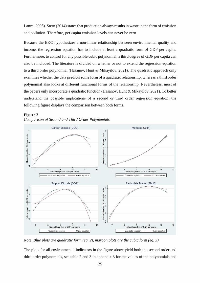
Because the EKC hypothesizes a non-linear relationship between environmental quality and

income, the regression equation has to include at least a quadratic form of GDP per capita.

Furthermore, to control for any possible cubic polynomial, a third degree of GDP per capita can

also be included. The literature is divided on whether or not to extend the regression equation

to a third order polynomial (Hasanov, Hunt & Mikayilov, 2021). The quadratic approach only

examines whether the data predicts some form of a quadratic relationship, whereas a third order

polynomial also looks at different functional forms of the relationship. Nevertheless, most of

the papers only incorporate a quadratic function (Hasanov, Hunt & Mikayilov, 2021). To better

understand the possible implications of a second or third order regression equation, the

following figure displays the comparison between both forms.

Figure 2

Comparison of Second and Third Order Polynomials

Note. Blue plots are quadratic form (eq. 2), maroon plots are the cubic form (eq. 3)

The plots for all environmental indicators in the figure above yield both the second order and

third order polynomials, see table 2 and 3 in appendix 3 for the values of the polynomials and

26

the turning points. The Y-axis represents the natural logarithm of the environmental indicator

and the X-axis the natural logarithm of GDP per capita. The range of the X-axis is based on the

minimum (6.741) and maximum (11.491) income of the sample, see table 4. The plots are based

on the following two fixed effects models:

ln 𝑌𝑖𝑡 = 𝛼𝑖 + 𝛿𝑡 + 𝛽1(𝑙𝑛𝐺𝐷𝑃𝑖𝑡) + 𝛽2(𝑙𝑛𝐺𝐷𝑃𝑖𝑡)2 + 𝑢𝑖𝑡 (2)

ln 𝑌𝑖𝑡 = 𝛼𝑖 + 𝛿𝑡 + 𝛽1(𝑙𝑛𝐺𝐷𝑃𝑖𝑡) + 𝛽2(𝑙𝑛𝐺𝐷𝑃𝑖𝑡)2 + 𝛽3(𝑙𝑛𝐺𝐷𝑃𝑖𝑡)3 + 𝑢𝑖𝑡 (3)

Where i represents the unit specific index and t the time specific index. Y represents the

environmental indicator (i.e. CO2, CH4, SO2 or PM10), αi is the unit specific intercept, δt the

time specific intercept and GDP per capita the economic growth variable. In addition, the

second order and third order of GDP per capita variable are also included to estimate the

polynomials. Finally, 𝑢𝑖𝑡 represents the error term. All variables are in natural logarithms.

Figure 2 shows that there is little difference between the two approaches. Although the

functional forms are relatively similar, the third order polynomial accounts for a greater variety

of possible functional forms. Therefore, this paper will focus on the third order polynomial

(equation 3) as the foundation of the method of analysis.

As discussed in section 2, this paper will also control for population density, trade openness

and time trends. In addition, the analysis will examine interaction effects. Normal control

variables control for the impact of these factors on the dependent variable. However, the EKC

hypothesis is more of a conditional correlation that projects a trend between environmental

quality and economic growth based on certain driving changes within society – e.g. structure

of the economy or technology as discussed in the theoretical framework –. Interaction terms

make it possible to control for the effects of these changes on the relationship rather than just

the level of the dependent variable (Brambor, Clark & Golder, 2006). Simply put, interaction

terms indicate whether the relationship of interest differs for different values of the interaction

variable. The interaction terms consists of the first and second order lnGDP per capita value

interacted with the control variables and time dummy variable. The empirical results are based

on the following 4 equations:

ln 𝑌𝑖𝑡 = 𝛼𝑖 + 𝛿𝑡 + 𝛽1(𝑙𝑛𝐺𝐷𝑃𝑖𝑡) + 𝛽2(𝑙𝑛𝐺𝐷𝑃𝑖𝑡)2 + 𝛽3(𝑙𝑛𝐺𝐷𝑃𝑖𝑡)3 + 𝛽4(𝑙𝑛𝑃𝑂𝑃𝐷𝑖𝑡) +

𝛽5(𝑙𝑛𝑇𝑅𝐴𝐷𝐸𝑖𝑡) + 𝑢𝑖𝑡 (4)

27

ln 𝑌𝑖𝑡 = 𝛼𝑖 + 𝛿𝑡 + 𝛽1(𝑙𝑛𝐺𝐷𝑃𝑖𝑡) + 𝛽2(𝑙𝑛𝐺𝐷𝑃𝑖𝑡)2 + 𝛽3(𝑙𝑛𝑃𝑂𝑃𝐷𝑖𝑡) + 𝛽4(𝑙𝑛𝑇𝑅𝐴𝐷𝐸𝑖𝑡) +

𝛽5(𝑙𝑛𝐺𝐷𝑃𝑙𝑛𝑃𝑂𝑃𝐷𝑖𝑡) + 𝛽6(𝑙𝑛𝐺𝐷𝑃2𝑙𝑛𝑃𝑂𝑃𝐷𝑖𝑡) + 𝑢𝑖𝑡 (5)

ln 𝑌𝑖𝑡 = 𝛼𝑖 + 𝛿𝑡 + 𝛽1(𝑙𝑛𝐺𝐷𝑃𝑖𝑡) + 𝛽2(𝑙𝑛𝐺𝐷𝑃𝑖𝑡)2 + 𝛽3(𝑙𝑛𝑃𝑂𝑃𝐷𝑖𝑡) + 𝛽4(𝑙𝑛𝑇𝑅𝐴𝐷𝐸𝑖𝑡)

+ 𝛽5(𝑙𝑛𝐺𝐷𝑃𝑙𝑛𝑇𝑅𝐴𝐷𝐸𝑖𝑡) + 𝛽6(𝑙𝑛𝐺𝐷𝑃2𝑙𝑛𝑇𝑅𝐴𝐷𝐸𝑖𝑡) + 𝑢𝑖𝑡 (6)

ln 𝑌𝑖𝑡 = 𝛼𝑖 + 𝛿𝑡 + 𝛽1(𝑙𝑛𝐺𝐷𝑃𝑖𝑡) + 𝛽2(𝑙𝑛𝐺𝐷𝑃𝑖𝑡)2 + 𝛽3(𝑙𝑛𝑃𝑂𝑃𝐷𝑖𝑡) + 𝛽4(𝑙𝑛𝑇𝑅𝐴𝐷𝐸𝑖𝑡)

+ 𝛽5(𝑙𝑛𝐺𝐷𝑃𝑙𝑛𝑇𝐼𝑀𝐸𝑖𝑡) + 𝛽6(𝑙𝑛𝐺𝐷𝑃2𝑙𝑛𝑇𝐼𝑀𝐸𝑖𝑡) + 𝑢𝑖𝑡 (7)

LnPOPD is the variable population density, lnTRADE the variable trade openness,

lnGDP(2)lnPOP the interaction terms of population density and lnGDP(2)lnTRADE the

interaction terms of trade openness. LnGDPTIME and lnGDP2TIME are the interaction terms

between different orders of GDP per capita and the time dummy variable that is equal to one

for all years after 1992. The inclusion of the control variables and interaction terms will be done

in separate models to increase the ease of interpretation. Furthermore, the models with the

interaction terms will be examined with only a quadratic function of GDP per capita for ease of

interpretation.

As mentioned above, a third order polynomial makes it possible to check the data for more

shapes than just an inverted U-shaped relationship. Lorente & Álvarez-Herranz (2016) give an

overview of the possible functional forms the EKC can exhibit2: (1) monotonically increasing

(β1 > 0, β2 = β3 = 0), (2) monotonically decreasing (β1 < 0, β2 = β3 = 0), (3) inverted U-shape (β1

> 0, β2 < 0, β3 = 0), (4) U-shape (β1 < 0, β2 > 0, β3 = 0), (5) N-shape (β1 > 0, β2 < 0, β3 > 0), (6)

an inverted N-shape (β1 < 0, β2 > 0, β3 < 0), or (7) no relationship or functional form (β1 = β2 =

β3 = 0). So, in order for an inverse U-shaped curve to occur, the coefficients need to β1 >

o; β2 < 0 & β3 = 0. In addition to this, the absolute value of β1 needs to be greater than the

absolute value of β2 (Friedl & Getzner, 2002).

Finally, when all coefficients display the expected sign and absolute size, the functional form

of an (inverted) U-shape or (inverted) N-shape yield turning points at certain levels of income

which indicate a change in the shape of the relationship. Diao et al. (2009) discuss how these

turning points can be found for four different functional forms (3, 4, 5 & 6). The turning point

estimations of this paper are based on these findings. All turning point estimations of Diao et

2 See figure 2 of Lorente & Álvarez-Herranz (2016) for variations in functional forms

28

al. (2009) are based on the outcome of a third order polynomial. However, this papers differs

in the fact that it uses the variables in their natural logarithmic form. In the case of an inverse-

U shaped curve or quadratic equation, the turning point (tp) can be found by the equation:

𝑡𝑝 = 𝑒−

𝛽12𝛽2 (6)

Similar to Stern (2014), a logarithmic polynomial has to take the exponent of the −𝛽1

2𝛽2 term in

order to calculate the turning point in US dollars. When the relationship displays an N-shaped

or inverse N-shaped curve, the calculation of the turning point is more complicated since there

are actually two turning points. Diao et al. (2009) find that the following equations for

calculating the turning points of an N-shaped curve:

𝑥1 = −𝛽2−√𝛽2−3𝛽1𝛽3

3𝛽3 𝑎𝑛𝑑 𝑥2 =

−𝛽2+√𝛽2−3𝛽1𝛽3

3𝛽3 (7)

Where x1 indicates the minimum turning point and x2 the maximum turning point3. However,

because this paper uses a function of natural logarithms, similar to equation 6, the turning points

of an N-shaped curve in this paper can be found by taking the natural exponent of these

outcomes to estimate the turning points in US dollars. This is supported by the outcome of the

plots in figure 2. Diao et al. (2009) also state that the turning points of an inverse N-shaped

curve can be calculated the same way as equation 7. However, applying this method on the

empirical results of this paper, I find that the calculation of the minimum and maximum turning

points for an inverse N-shaped curve are reversed. This leads to the following equation:

𝑥1 = −𝛽2 + √𝛽2 − 3𝛽1𝛽3

3𝛽3

𝑎𝑛𝑑 𝑥2 = −𝛽2 − √𝛽2 − 3𝛽1𝛽3

3𝛽3

(8)

Again, it is important to note that in order to calculate the turning points in US dollars the

natural exponent of these outcomes needs to be calculated. Finally, for both equation 7 and 8

the turning points may not exist for the corresponding curve. This will be indicated with N.A.

in the empirical results tables.

3 See figure 2 of Lorente & Álvarez-Herranz (2016) for a visual explanation

29

3.4 Reliability and Validity

The main issue with the scientific literature on the existence of an EKC, is the endogeneity

problem. While some economists argue that there is a causal relationship between

environmental quality and income, most economist argue that there is only a conditional

correlation because of omitted variable bias (Lin & Liscow, 2012). Rather than income causing

environmental degradation or improvement, the two factors move together and only display a

relationship because of various underlying societal changes. Lin & Liscow (2012) therefore

discuss two endogeneity problems regarding the EKC literature. First, the problem of reversed

causality. Instead of a change in emission and pollution as the result of an increase in income

driven by societal changes, the reversed relationship can also be true. For example, increases in

emission and pollution due to more production can result in a higher level of income. Second,

the authors argue, endogeneity is the result of omitted variable bias. While controlling for

different variables can help reduce this endogeneity problem, it is almost impossible to rule out

any other important factors that causes both economic growth and emissions (Lin & Liscow,

2012). This problem is inherent to the EKC hypothesis and should therefore always be

considered when interpreting any results. Rather than explain any causality, this paper aims to

shine some light on the conditional correlation where income and environmental quality move

together conditional on some societal changes. However, with the aim of limiting the problem

of endogeneity in this paper, the analysis uses interaction terms to filter out the effect of the

hypothesized influential factors.

The method of this paper has a high level of reliability. All the data are extracted from reliable

datasets that are compiled by renowned (public) research institutions. The operationalization of

the variables follows the international standards used in most of the energy economics literature.

The method of data collection and method of analysis are discussed transparently so that

reproduction of the research by following the outlined steps is relatively easy. The choice of

method is done through the Sargan-Hansen overidentifying test, which indicates the method

that best fits the data; random effects or fixed effects. This increases the reliability of the study

by limiting any personal bias towards a statistical model and results in a more objective method

of analysis. Moreover, the fixed effects models are tested for time-fixed effects trends by the

STATA testparm command and adjusted accordingly.

A limitation of this research is the limited internal validity of the theory. As explained in the

sections above, the Environmental Kuznets Curve is mainly a statistical and empirical

30

occurrence, rather than a hard theoretical causal mechanism (Stern, 2017). The interest of the

research on this topic is more focused on finding a development path that describes a country’s

development through the relationship between environmental quality and income (Selden &

Song, 1994). Although careful consideration on the variable conceptualization,

operationalization and possible control variables ensures some of the internal validity, the

reality of the EKC endogeneity problem limits the internal validity inevitably.

Another limitation is the operationalization of all the dependent variables other than CO2 per

capita. Greenhouse gases and air pollution measures are often transformed into their equivalent

quantity in levels of CO2, which is not the case for this study. However, the independent variable

unit of measurement is similar for all models and indicators, so the expected effect of a lower

turning point for air pollution measures can still be accounted for.

31

4. Analysis

This chapter will discuss the descriptive statistics and empirical analysis. Thereafter, all data

will be examined in relation to the research question.

4.1 Descriptive Statistics

Table 4 presents the descriptive statistics of all the included variables. In order to better interpret

the size of the variables, both the original unit of measurement and the coefficients of the natural

logarithm are summarized. The data includes 41 different countries4 from the regions of Europe,

Asia, North-America, South-America, Oceania, the Middle East and Africa. The timeframe of

the study ranges from 1970 to 2015, a total of 46 years. Only the GDP per capita variable is

included and the descriptive statistics of the quadratic and cubic values of GDP per capita are

left out because the ease of interpretability for these values is lost.

The dataset is strongly balanced and includes four different indicators of environmental quality:

CO2, CH4, SO2, and PM10. All dependent variables have 1886 observations (41 x 46) with the

exception of CO2 per capita levels. This variable has two missing values for the year 2015 and

the countries France and Japan. As discussed in the previous section, the unit of measurements

of these variables is metric ton per capita. Out of all four dependent variables, CO2 per capita

has the largest mean and PM10 the smallest. CO2 is the most emitted greenhouse gas of the

selection and SO2 the most emitted air polluter. Moreover, both greenhouse gas measures have

a larger mean, standard deviation, minimum, median and maximum than the air pollution

measures. This means that there are substantially more greenhouse gases emitted than air

polluters. All dependent variables are skewed to the left, as the means are greater than the

medians.

The main explanatory variable of interest is income, measured by GDP per capita. The mean

income of the sample is 21 879 US dollars. The standard deviation of 15 650 US dollars is

rather large and shows the large variation of income within the sample, contrary to many

previous studies that mostly focus on the more concentrated range of income of developing

countries. The inclusion of countries with a large variation in income increases the explanatory

power of the model. The other independent variables also have a very large variation. The

4 See Appendix 1 for a full list of all the included countries

32

summarized statistics of the natural logarithms are displayed in the lower part of the table, to

improve the readability of the coefficients in the later empirical results section.

Table 4: Descriptive Statistics

Obs Mean Std. Dev. Min Median Max

Variables (1) (2) (3) (4) (6) (5)

CO2 per capita 1884 6.717 5.527 0.308 5.946 40.589

CH4 per capita 1886 0.108 0.139 0.0165 0.065 0.941

SO2 per capita 1886 0.031 0.0373 0.001 0.019 0.274

PM10 per capita 1886 0.010 0.010 6.31e-07 0.006 0.052

GDP per capita 1886 21879 15650 846 19088 97864

Population

Density 1886 105.125 118.666 1.628 64.986 524.526

Trade Openness 1886 60.285 41.369 0.021 52.617 408.368

lnCO2pc 1884 1.517 0.980 -1.176 1.783 3.704

lnCH4pc 1886 -2.629 0.805 -4.106 -2.733 -0.061

lnSO2pc 1886 -4.028 1.056 -6.647 -3.984 -1.295

lnPM10pc 1886 -5.471 2.023 -14.276 -5.088 -2.951

lnGDPpc 1886 9.671 0.904 6.741 9.857 11.491

lnPOPden 1886 3.932 1.361 0.487 4.174 6.261

lnTrade 1886 3.906 0.681 -3.863 3.963 6.012

33

Table 5 displays the average values of the whole sample over time for all the dependent and

independent variables. The dependent variable CO2 per capita shows neither an increasing nor

a decreasing trend. The levels first increase, then decrease and finally increase again. The

dependent variable CH4 per capita, however, shows a downward trend in the average per capita

emissions over the years for the entire sample. Similarly, both air pollution measures display a

negative trend in per capita pollution levels for the sample as a whole. Income increases over

all years and almost doubles in size. The remaining independent variables also show a strong

increase over time, meaning that the sample as a whole has become more densely populated

and increased the levels of trade openness.

Table 5: Descriptive Statistics Change in Dependent Variables Over Time

1970-80 1981-90 1991-2000 2001-10 2011-2015

Variables (1) (2) (3) (4) (5)

CO2 per capita 6.641 6.525 6.766 7.152 6.608

CH4 per capita 0.128 0.120 0.103 0.098 0.095

SO2 per capita 0.044 0.039 0.028 0.020 0.018

PM10 per capita 0.010 0.010 0.010 0.009 0.009

GDP per capita 15520 17145 22243 27798 29901

Population Density 85.698 91.547 107.883 119.867 129.101

Trade Openness 48.189 50.819 58.810 73.017 79.405

lnCO2pc 1.353 1.397 1.570 1.667 1.658

lnCH4pc -2.450 -2.516 -2.669 -2.751 -2.781

lnSO2pc -3.700 -3.770 -4.011 -4.353 -4.495

lnPM10pc -5.476 -5.442 -5.440 -5.525 -5.545

lnGDPpc 9.335 9.438 9.701 9.949 10.078

lnPOPden 3.679 3.769 3.986 4.108 4.188

lnTrade 3.683 3.755 3.857 4.147 4.207

34

For a visual overview of the EKC relationship by country, see appendix 2. Even though this is

a lot of information to take in, it is very helpful to see a plot of the EKC relationship per country

to better understand the large variety of data. Most countries seem to display some relationship

between environmental quality and income. Exceptions are Algeria, Argentina, Iran, Iraq,

Philippines and South Africa. For this selection of countries, there does not seem to be any

development path or trend. Upon closer inspection of the graphs, Australia, Indonesia, France

and United Kingdom seem to show some sign of an inverse U-shaped development path for all

four measures and with the addition of Belgium and Japan for the air pollution measures SO2

and PM10. Some different development paths can also be seen, for example monotonically

increasing, U-shaped or N-shaped.

35

4.2 Empirical Results Greenhouse Gases

Table 6 Fixed Effects Carbon Dioxide (CO2) per capita

Variable (1) (2) (3) (4)

GDP per capita -15.656***

(1.019)

4.674***

(0.666)

5.523***

(0.156)

3.216***

(0.168)

(GDP per capita)2 2.020***

(0.112)

-0.224***

(0.034)

-0.294***

(0.011)

-0.145***

(0.009)

(GDP per capita)3 -0.082***

(0.004) - - -

Population Density -0.051**

(0.024)

0.128

(0.715)

-0.008

(0.026)

-0.059**

(0.025)

Trade Openness -0.068***

(0.010)

-0.069***

(0.012)

-1.657***

(0.178)

-0.071***

(0.012)

GDP*Population Density - -0.016

(0.145) - -

GDP2*Population Density - 1.05e-5

(0.007) - -

GDP*Trade Openness - - 0.183***

(0.020) -

GDP2*Trade Openness - - -2.32e-5***

(3.19e-6) -

GDP*Time 2.507***

(0.187)

GDP2*Time -0.137***

(0.010)

Constant 38.673***

(3.059)

-22.339***

(3.265)

-21.883***

(0.577)

-15.537

(0.751)

R2 0.556 0.542 0.523 0.554

Sargan-Hansen 0.000 0.000 0.000 0.000

Turning Point ex1 = N.A.

ex2 = 25 765 33 963 12 002 65 490

Country Effects Yes Yes Yes Yes

Time Effects Yes Yes Yes Yes

N 41 41 41 41

N x T 1884 1884 1884 1884

Note: Variables are in natural logarithms. Standard errors in parentheses. Significance

*p<0.10, **p<0.05, ***p<0.01. Sargan-Hansen values are p-values of test statistic. Turning

points in US dollars.

36

The empirical results of the greenhouse gas CO2 are displayed in table 6. The table includes

four models. All variables are in natural logarithms because of the large values and the non-

zero restriction. The dependent variable is the natural logarithm of CO2 emissions per capita,

which is an indicator of environmental quality. The control variables are natural logarithms of

population density (people per square kilometre of land area), trade openness (trade as a

percentage of GDP) and a time dummy variable that is 0 for years before 1993 and 1 for all

years after 1992. From this point onwards, the discussion of the output will be spoken of without

mentioning the fact that the coefficients are scaled to natural logarithms to improve readability.

Model 1 yields the estimates of equation 4 with just the environmental quality – income

relationship and the control variables population density and trade openness. The following

three models are all estimated with a second order polynomial to ease the interpretation of the

interaction terms. Model 2 yields the estimates of equation 5 where the interaction terms of the

variable population density are added. Model 3 yields the estimates of equation 6 in which the

interaction terms of the variable trade openness are added. Finally, model 4 includes two

interactions with a time variable that is 0 for 1970 to 1992, and 1 for all years after 1992 to

control for time trends.

The Sargan-Hansen coefficients show the results of the overidentifying tests and examine

whether a fixed effects model or random effects model is the best fit. The coefficients are the

p-values of the test statistic. The null hypothesis states that the regressor is uncorrelated with

the group-specific error term and therefore a random effect model is the best fit. The alternative

hypothesis states that the regressors are uncorrelated with the idiosyncratic error term (for both

year and country specific values) and that a fixed effects model should be used (Schaffer &

Stillman, 2010). The outcome of the Sargan-Hansen test in all models is in favour of the fixed

effects regression model with p-values smaller than 0.01.

In model 1, GDP per capita is negative in direction and statistically significant. The squared

GDP per capita is positive and statistically significant and the cubed coefficient is again

negative and statistically significant. In addition, the absolute value of GDP per capita is greater

than the absolute value of the squared coefficient. However, the coefficients do not follow the

expected direction of an inverse U-shaped curve where β1 > 0, β2 < 0 and β3 = 0. The model

shows reversed signs for β1 (< 0), β2 (> 0) and β3 (< 0). Therefore, the CO2 EKC relationship

has the functional form of an inverted N-shaped curve. Both control variables are negative and

statistically significant. This means that a higher population density results in less CO2 emission

per capita. Additionally, higher levels of trade openness also result in less CO2 per capita

37

emissions. The turning point (X2) of the concave parabolic part of the inverse N-shaped curve

is 25 765 US dollars. 25 765 US dollars is equal to ln(25 765) = 10.16. In comparison to the

outcomes of figure 2 and table 3 (appendix 3), the turning point increases with the inclusion of

population density and trade openness.

Model 2 introduces the interaction terms based on the variable population density. With the

inclusion of these interaction terms, population density becomes insignificant. Trade openness

remains statistically significant and negative in direction. Both population density interaction

terms are not statistically significant.

Model 3 introduces the trade openness interaction terms. Similarly to model 2, population

density is not significant and trade openness is negative and significant. More notably, both

interaction terms are statistically significant. The interaction between trade openness and GDP

per capita is positive, meaning that there is a difference between countries with high levels of

trade openness and low levels. More specifically, in countries with high levels of relative trade

openness the effect of GDP per capita on CO2 emissions per capita is larger. The interaction

term with the squared GDP per capita variable and trade openness is negative and, thus, the

relationship has a stronger curvature for high levels of trade openness.

Model 4 introduces the time interaction effects with a time dummy that is 1 for all years larger

than 1992. Population density becomes statistically significant, similar to model 1. Trade

openness maintains significance and the negative sign. The time interaction terms are both

statistically significant. The interaction with GDP per capita has a positive sign and the

interaction with the squared GDP per capita has a negative sign. This former means that for the

years after 1992, GDP per capita has a larger effect on CO2 per capita emissions. The latter

means that the curvature of the CO2 EKC is stronger in the years after 1992.

Finally, there is large variation in the turning points. However, this paper mainly focuses on the

turning point of model 1 for comparison between indicators. The difference between the model

in the order of polynomials makes it unreliable to compare the turning points between model 1

and the following models. Looking at only model 2, 3 and 4 the table shows the largest turning

point for the time trend model and the lowest for the population density interaction model (2).

38

Table 7 Fixed Effects Methane (CH4) per capita

Variable (1) (2) (3) (4)

GDP per capita 1.295

(1.122)

-3.127***

(0.636)

-0.992***

(0.157)

-0.580***

(0.178)

(GDP per capita)2 -0.160

(0.124)

0.206***

(0.032)

0.074***

(0.011)

0.050***

(0.010)

(GDP per capita)3 0.008*

(0.005) - - -

Population Density -0.169***

(0.026)

-2.326**

(0.682)

-0.174***

(0.026)

-0.173***

(0.026)

Trade Openness 0.030**

(0.012)

0.023**

(0.011)

0.033

(0.179)

0.030***

(0.012)

GDP*Population Density - 0.537***

(0.139) - -

GDP2*Population Density - -0.034***

(0.007) - -

GDP*Trade Openness - - 0.003

(0.020) -

GDP2*Trade Openness - - -1.84e-5***

(2.31e-6) -

GDP*Time - - - -0.411**

(0.198)

GDP2*Time - - - 0.21**

(0.010)

Constant -6.407*

(3.367)

9.216***

(3.117)

0.794

(0.580)

-0.848

(0.796)

R2 0.150 0.130 0.145 0.151

Sargan-Hansen 0.000 0.000 0.000 0.000

Turning Point N.A. 1 978 N.A. N.A.

Country Effects Yes Yes Yes Yes

Time Effects Yes Yes Yes Yes

N 41 41 41 41

N x T 1886 1886 1886 1886

Note: Variables are in natural logarithms. Standard errors in parentheses. Significance *p<0.10,

**p<0.05, ***p<0.01. Sargan-Hansen values are p-values of test statistic. Turning points in US

dollars.

39

The empirical results of the greenhouse gas CH4 are displayed in table 7. All models are the

same as the models of table 6. The dependent variable is the natural logarithm of CH4 per capita,

which is an indicator of environmental quality. The control variables are the natural logarithms

of population density (people per square kilometre of land area), trade openness (trade as a

percentage of GDP) and a dummy variable time trend that is 0 for the years before 1993 and 1

for all years after 1992. From this point onwards, the discussion of the output will be spoken of

without mentioning the fact that the coefficients are scaled to natural logarithms to improve

readability.

The Sargan-Hansen coefficients show the results of the overidentifying tests and examine

whether a fixed effects model or random effects model is the best fit. The outcome of the

Sargan-Hansen test in all models is in favour of the fixed effects regression model with p-values

smaller than 0.01.

In model 1, none of the GDP per capita variables (first order, squared or cubic) display any

significance at the 95% confidence level of higher. Although, model 2, 3 and 4 show

significance for GDP per capita and squared GDP per capita, the significance disappears when

a third order GDP per capita variable is added. Therefore, the results do not show a relationship

in any form between CH4 per capita emissions and GDP per capita. All four models show

statistically significant negative effect of population density on CH4 per capita emissions,

meaning that more densely populated countries have lower emissions of CH4 per capita.

Moreover, with the exception of model 3, trade openness is statistically significant with a

positive sign. This means that higher levels of trade openness increase the CH4 per capita levels.

Moreover, model 2 shows a positive sign for the interaction term between population density

and GDP per capita, meaning that the effect of GDP per capita on CH4 emissions is larger in

more densely populated countries. The interaction term between population density and squared

GDP per capita is negative, meaning that the curvature of the relationship is stronger for higher

levels of population density. However, note that the curved relationship is not present in the

third order polynomial. Model 3 shows that only the interaction term between trade openness

and the squared GDP per capita variable is significant and negative in direction. Meaning that

the relationship has a stronger curvature for high levels of trade openness. Finally, the

interaction terms in model 4 are both significant with a negative and positive sign, respectively.

Therefore, GDP has a smaller effect on CH4 emissions per capita in the years after 1992 and

the curvature of the relationship weaker in the years after 1992.

40

4.3 Empirical Results Air Pollution Measures

Table 8 Fixed Effects Sulphur Dioxide (SO2) per capita

Variable (1) (2) (3) (4)

GDP per capita -27.906***

(2.157)

9.144***

(1.346)

10.171***

(0.322)

5.861***

(0.345)

(GDP per capita)2 3.632***

(0.238)

-0.454***

(0.069)

-0.610***

(0.023)

-0.309***

(0.019)

(GDP per capita)3 -0.152***

(0.009) - - -

Population Density -0.027

(0.050)

0.485

(1.445)

0.048

(0.053)

-0.087*

(0.051)

Trade Openness -0.153***

(0.022)

-0.173***

(0.024)

-2.853***

(0.367)

-0.158***

(0.022)

GDP*Population Density - 0.086

(0.294) - -

GDP2*Population Density - -0.014

(0.015) - -

GDP*Trade Openness - - 0.316***

(0.042) -

GDP2*Trade Openness - - -6.42e-5***

(6.57e-6) -

GDP*Time - - - 4.273***

(0.383)

GDP2*Time - - - -0.242***

(0.020)

Constant 64.687***

(6.474)

-48.792***

(6.601)

-45.38***

(1.190)

-30.357***

(1.544)

R2 0.108 0.079 0.069 0.078)

Sargan-Hansen 0.000 0.000 0.000 0.000

Turning Point ex1 = N.A.

ex2 = 12 867 23 635 4 175 13 145

Country Effects Yes Yes Yes Yes

Time Effects Yes Yes Yes Yes

N 41 41 41 41

N x T 1886 1886 1886 1886

Note: Variables are in natural logarithms. Standard errors in parentheses. Significance

*p<0.10, **p<0.05, ***p<0.01. Sargan-Hansen values are p-values of test statistic. Turning

points in US dollars.

41

The empirical results of the air pollution measure SO2 are displayed in table 8. All models are

the same as the models in the previous tables. The dependent variable is the natural logarithm

of SO2 emissions per capita, which is an indicator of environmental quality. The control

variables are the natural logarithms of population density (people per square kilometre of land

area), trade openness (trade as a percentage of GDP) and a time dummy variable that is 0 for

the years before 1993 and 1 for all years after 1992. From this point onwards, the discussion of

the output will be spoken of without mentioning the fact that the coefficients are scaled to

natural logarithms to improve readability

The Sargan-Hansen coefficients show the results of the overidentifying tests and examine

whether a fixed effects model or random effects model is the best fit. The outcome of the

Sargan-Hansen test in all models is in favour of the fixed effects regression model with p-values

smaller than 0.01.

In model 1, GDP per capita is negative in direction and statistically significant. The squared

GDP per capita is positive and statistically significant and the cubed coefficient is negative and

statistically significant. In addition, the absolute value of GDP per capita is greater than the

absolute value of the squared coefficient. However, the coefficients do not follow the expected

direction of an inverse U-shaped curve where β1 > 0, β2 < 0 and β3 = 0. The model shows

reversed signs for β1 (< 0), β2 (> 0) and β3 (< 0). Therefore, the SO2 EKC relationship has the

functional form of an inverted N-shaped curve. The population density variable does not display

significance at the 95% confidence level or higher in any of the four models. Trade density is

statistically significant in all models and negative in direction. This means that higher levels of

trade openness result in less SO2 per capita emissions. The turning point (X2) of the concave

parabolic part of the inverse N-shaped curve is 12 867 US dollars. This is equal to ln(12 867)

= 9.46. In comparison to the outcomes of figure 2 and table 3 ( appendix 3), the turning point

increases with the inclusion of population density and trade openness.

Model 2 introduces the interaction terms based on the variable population density. However,

the corresponding coefficients are not statistically significant.

Model 3 introduces the trade openness interaction terms. The interaction of trade openness with

GDP per capita is positive, meaning that there is a difference between countries with high levels

of trade openness and low levels. More specifically, in countries with high levels of trade

openness the effect of GDP per capita on SO2 emissions per capita is larger. The interaction

42

term with squared GDP per capita is and trade openness is negative. This means that the

curvature is stronger at high levels of trade openness.

Model 4 introduces the time interaction effects with a time dummy that is 1 for all years later

than 1992. The time interaction terms are both statistically significant. The interaction with

GDP per capita has a positive sign and the interaction with the squared GDP per capita has a

negative sign. This former means that for the years after 1992, GDP per capita has a larger

effect on CO2 per capita emissions. The latter means that the curvature of the SO2 EKC is

stronger in the years after 1992.

Finally, SO2 also shows a large variation in turning points. However, this paper mainly focuses

on the turning point of model 1 for comparison between indicators. The difference in the order

of polynomials between the models makes it unreliable to compare the turning points between

model 1 and the following models. Looking at only model 2, 3 and 4 the table shows the largest

turning point for model 2 and the smallest for model 3.

43

Table 9 Fixed Effects PM10 (PM10) per capita

Variable (1) (2) (3) (4)

GDP per capita 3.738**

(1.876)

12.332***

(1.080)

3.066***

(0.261)

1.070***

(0.295)

(GDP per capita)2 -0.304

(0.207)

-0.621***

(0.055)

-0.195***

(0.019)

-0.050***

(0.017)

(GDP per capita)3 0.008

(0.008) - - -

Population Density -0.227***

(0.043)

11.262***

(1.159)

-0.216***

(0.043)

-0.261***

(0.044)

Trade Openness -0.097***

(0.019)

-0.121***

(0.019)

-1.546***

(0.298)

-0.095***

(0.019)

GDP*Population Density - -2.338***

(0.236) - -

GDP2*Population Density - 0.118***

(0.012) - -

GDP*Trade Openness - - 0.161***

(0.034) -

GDP2*Trade Openness - - 1.117e-5**

(5.32e-6) -

GDP*Time - - - -1.056***

(0.328)

GDP2*Time - - - 0.050***

(0.017)

Constant -18.939***

(5.630)

-65.046***

(5.295)

-16.091***

(0.966)

-9.798***

(1.320)

R2 0.040 0.032 0.052 0.045

Sargan-Hansen 0.757 0.833 0.301 0.653

Turning Point ex1 = 36 316

ex2 = N.A. 20 520 2 596 44 356

Country Effects Yes Yes Yes Yes

Time Effects Yes Yes Yes Yes

N 41 41 41 41

N x T 1886 1886 1886 1886

Note: Variables are in natural logarithms. Standard errors in parentheses. Significance

*p<0.10, **p<0.05, ***p<0.01. Sargan-Hansen values are p-values of test statistic. Turning

points in US dollars.

44

The empirical results of the air pollution measure PM10 are displayed in table 9. All models

are the same as the models in the previous tables. The dependent variable is the natural

logarithm of PM10 emissions per capita, which is an indicator of environmental quality. The

control variables are the natural logarithms of population density (people per square kilometre

of land area), trade openness (trade as a percentage of GDP) and a time dummy variable that is

0 for years before 1993 and 1 for all years after 1992. From this point onwards, the discussion

of the output will be spoken of without mentioning the fact that the coefficients are scaled to

natural logarithms to improve readability.

The Sargan-Hansen coefficients show the results of the overidentifying tests and examine

whether a fixed effects model or random effects model is the best fit. The outcome of the

Sargan-Hansen test is in favour of a random effects model. However, to better compare the

effects with all the other environmental indicators and because the coefficients are relatively

similar to the random effects models5 in terms of size and significance, the fixed effects

estimates are presented here and the random effects models in appendix 4.

In model 1, only the first order GDP per capita is statistically significant at the 95% confidence

level. Whereas, model 2, 3 and 4 show significance for GDP per capita and the squared GDP

per capita, the significance disappears when controlling for a third order GDP per capita

variable. This is opposite to the plot of PM10 in figure 2, which does display an inverse U-

shaped curve. The results of table 9 only show a monotonically increasing relationship between

PM10 and GDP per capita. Models 1, 2 and 4 show a negative significant effect of population

density on PM10 per capita emissions, meaning that more densely populated countries have

lower emissions of PM10 per capita. Model 3 shows the opposite for population density.

Moreover, trade openness is statistically significant with a negative sign. This means that higher

levels of trade openness decrease PM10 per capita.

Model 2 shows a negative sign for the interaction term between population density and GDP

per capita, meaning that the effect of GDP per capita on PM10 per capita is smaller in more

densely populated countries. The interaction term between population density and the squared

GDP per capita is positive, meaning that the curvature of the relationship is weaker for more

densely populated areas. However, note that the curved relationship is not present in the third

order polynomial of table 9, it does however in model 10 (appendix 4).

5 See Appendix 4 for the Random Effects estimates of PM10

45

Model 3 shows that both interaction term of trade openness are significant and positive in

direction. This means that in countries with higher levels of trade openness, the effect of GDP

on PM10 emissions is larger and the curvature of this relationship is weaker for countries with

high levels of trade openness.

Model 4 introduces the time interaction effects. The time interaction terms are both statistically

significant. The interaction with GDP per capita has a negative sign and the interaction with the

squared GDP per capita has a positive sign. The former means that for the years after 1992,

GDP per capita has a smaller effect on PM10 per capita emissions. The latter means that the

curvature between PM10 and GDP per capita is weaker in the years after 1992.

However, please note that in model 1 of table 10, the squared variable of GDP per capita is

statistically significant at the 90 % confidence level. This means that this random effects model

does find an inverse U-shaped relationship. This will be discussed in the hereafter following

analysis.

46

4.4 Empirical Analysis

Tables 6 through 9 display the results for the individual environmental indicators. However, the

aim of this paper is to see how these indicators differ and why. Therefore, this section will

discuss and analyse the main similarities and differences between the greenhouse gases and air

pollution measures.

None of the fixed effects tables show an inverse U-shaped path in the third order polynomial

regression models where β1 > 0, β2 < 0 and β3 = 0. PM10 per capita has a monotonically

increasing relationship in model 1 of table 9. However, this relationship changes to an inverse

U-shaped relationship in the random effects model6 of table 10, with a 90% confidence level.

The turning point of this curve is 17 283 US dollars. The Sargan-Hansen test statistic confirms

that this random effects model is a better fit and is therefore more robust. The conclusion and

analysis will focus on the random effects model of PM10.

Even though no other environmental indicators show the correct sign for an inverse U-shaped

relationship, both CO2 per capita and SO2 per capita show an inverse N-shaped relationship

with GDP per capita in the third order polynomial models. The corresponding turning point of

CO2 is 25 765 US dollars. For SO2 per capita, the turning point is 12 867 US dollars. The

greenhouse gas CH4 does not show an inverse U or N shaped relationship with GDP per capita

in model 1 of table 7 and, therefore, does not have a turning point.

The significant findings of the inverse U and N-shaped functional forms mean that the first

alternative hypothesis (H1) can be accepted: higher economic growth yields lower emission

and pollution when certain conditions are met. Moreover, the turning point of the greenhouse

gas CO2 per capita (25 765 US$) is higher than the turning points of the air pollution measures

SO2 per capita (12 867 US$) and PM10 per capita (17 283 US$). Therefore, the fifth alternative

hypothesis (H5) can be accepted: the turning points for air pollution measures are at lower levels

of GDP per capita than the turning points of greenhouse gases. The results confirm H5 for CO2,

SO2 and PM10.

The variable population density is statistically significant and negative in direction in all

models, except for SO2 (table 8). This means that in countries with high population density,

GDP per capita has a larger effect on CO2, CH4 and PM10. This is in line with the fourth

6 Appendix 4

47

hypothesis (H4): higher population density yields less emission and pollution. The empirical

results confirm H4 for CO2, CH4 and PM10.

However, it is strange that population density does not have an effect on SO2 per capita, but

does affect CO2 per capita. The main sources of SO2 and CO2 are similar: fossil fuel combustion

for energy production, transportation, and industry (EPA, 2019, 2020). However, the CO2 per

capita emissions are substantially larger than the SO2 per capita emissions, see table 4 and 5.

This means that CO2 per capita emissions increase much more in absolute terms in comparison

to SO2 per capita emission when the sources that result in these emissions change. Moreover,

the results do show similar results for SO2 per capita and CO2 per capita regarding the two

interaction terms of population density. There is no difference between countries with different

levels of population density for both environmental indicators.

The interaction terms of population density for CH4 and PM10 show a positive interaction with

GDP per capita for CH4 (in densely populated countries, the effect of GDP per capita on CH4

emissions is larger) and a negative interaction with GDP per capita for PM10 (in densely

populated countries, the effect of GDP per capita is smaller). This is a logical outcome in

comparison to the sources of the emissions. In more densely populated areas income is

generally higher, and higher levels of income lead to more consumption of natural gas systems

through cooking or showering, resulting in more CH4 emissions. Higher population density also

asks for mood for and therefore livestock. PM10 is an air pollutant and in a more densely

populated area, there is probably more emphasis on improving air quality and reducing haze

when income is high, because the effects are more immediate.

Trade openness has a negative effect on CO2 per capita, SO2, per capita and PM10 per capita

emissions. This means that these emission go down when the relative trade openness of a

country (imports + exports as a share of GDP) increases. This is in line with the second

hypothesis (H2): higher trade openness yields less emission and pollution for these three

indicators. The results confirm H2 for CO2, SO2, and PM10. However, for CH4, higher trade

openness results in more CH4 emissions. This could be due to more livestock for export or

larger landfills due to a larger supply of consumption goods, which increase waste and therefore

methane.

The interaction term between trade openness and GDP per capita is positive and significant for

the same three indicators, and insignificant for CH4 per capita. The second interaction term of

trade openness with squared GDP per capita is negative for CO2 per capita, CH4 per capita, and

48

SO2 per capita. Contrary to a positive interaction term for PM10 per capita. Since CH4 does not

display a second or third degree polynomial, this means that CO2 and SO2, have stronger

curvatures for the EKC relationship at higher levels of trade openness, and PM10 a weaker

curvature.

Finally, the time interactions are similar for CO2 and SO2, and similar but opposite in direction

for CH4 and PM10. The outcome for the first interaction terms means that the effect of GDP

per capita on CO2 per capita and SO2 per capita is larger in the years after 1992. For CH4 and

PM10, the effect of GDP per capita on CH4 per capita and PM10 per capita is smaller in the

years larger than 1992. The second time interaction term shows that the curvature of CO2 and

SO2 is stronger in the years after 1992 and weaker for CH4 and PM10.

The final relationship between all environmental indicators and GDP per capita are displayed

in figure 3 below. These plots are based on model 1 of the respective empirical results table for

the first three indicators CO2, CH4 and SO2. The plot of PM10 is based on the model 1

coefficients of table 10, appendix 4.

Figure 3

Comparison of Second and Third Order Polynomials

Note. Plot of PM10 is based on RE regression, appendix 4.

49

The turning points of CO2 is 25 765 US dollars. This is equal to ln(25765) = 10.16. This turning

point is in line with plot 1. For SO2, the turning point is equal to ln(12867) = 9.46, which is in

line with the third plot. The aforementioned turning point of PM10 in table 10 is equal to

ln(17282) = 9.75. This finding is based on a confidence level of 90 and in line with plot 4 of

figure 3.

50

5. Conclusion

The economic concept of an Environmental Kuznets Curve hypothesizes an inverse U-shaped

relationship between environmental quality and economic growth. This relationship represents

a development path between these two factors that argues that environmental quality

deteriorates in the early stages of economic development where industry expands and uses dirty

and cheap materials. With societal changes driving economic growth, the environmental

damage diminishes up to an intermediate level of income. After this income level has been

reached, the hypothesis argues that further economic growth can result in improvements in

environmental quality. This paper focuses on explaining how these changes in society drive

economic growth and the relationship with environmental quality. A better understanding of

the existence of a development path between income and environmental quality can help

provide a baseline scenario and framework for environmental policy.

Research on the topic of the EKC hypothesis is extensive but still mixed and inconclusive.

Furthermore, research design and selected data varies among academic articles. In general the

consensus in the academic literature on the relevance of the EKC is not disputed, but the proxy

of environmental quality is. Most often, these proxies are either greenhouse gases or air

pollution measures. This paper aims to close the gap in the research of the lack of more recent

international research into the comparison between the EKC for both greenhouse gases and air

pollution measures. Therefore, the analysis includes four dependent variables that proxy

environmental quality: the two greenhouse gases CO2 & CH4, and the two air polluters SO2 and

PM10. Greenhouse gases are the main cause of global warming and climate change, whereas

air pollution measures are more a concern of affecting public health. Additionally, air polluters

can also contribute to climate change by leading to acid rain for example.

The sample includes 41 different countries for the years 1970 to 2015. The existence of an

inverse U-shaped curve is assessed on the most appropriate random of fixed effects model, after

a Sargan-Hansen overidentifying test. The control variables are population density, trade

openness and the inclusion of a time interaction model. Both control variables are also

interacted with income to control for changes in the slope or curvature of the relationship.

The largest limitation of the EKC is the endogeneity problem. Rather than a causal relationship,

the development trend is more of a conditional correlation because there is the problem of

reversed causality where emissions might cause changes in income. Moreover, the problem of

endogeneity stems from omitted variable bias. This is an inherent problem to the concept of the

51

EKC and should always be taken into account when interpreting any results. The inclusion of

interaction aims to limit some of endogeneity problems. The reliability of this paper is high.

The data are extracted from renowned research institutions and the method is clearly and

transparently discussed.

The theoretical assumptions as to why economic growth can lower emission levels, are

described in the static model. This models assumes that emission in an economy increases when

(i) economies develop and expand, (ii) the more difficult it is to substitute the pollution for other

inputs, and (iii) when it is easy to increase utility by consuming more at the expense of the

environment. The opposite effects can thus result in a reduction of emissions. Additionally,

three other effects describe the theoretical mechanisms for the possibility of an inverse U-

shaped relationship. The scale effect describes the expansion of industry and increase in

resource depletion and emissions. This effect is countered by the composition effect and

technique effect. The former concerns the effect of different sectors in an economy. Agriculture

and heavy industry are more polluting than service and information sectors. Furthermore, the

technique effect assumes that more efficient technology and improvements in environmental

policy can also help reduce emissions.

To analyse these theoretical implications for the four environmental indicators, the paper

focuses on answering the following research question: to what extent and why does the effect

of economic development on greenhouse gas emissions differ from the effect of economic

development on air pollution?

The empirical results and analysis shows many differences but also a some similarities. PM10

is the only environmental indicator that displays an inverse U-shaped relationship, this is due

to the fact that the effects of PM10 (haze or smoke) are very noticeable and relatively cheap to

abate. Additionally, rather than similar effects for the group greenhouse gases and the group air

polluters with difference between the two categories, the findings show that CO2 and SO2

display a very similar development trend. Both indicators display an inverse N-shaped EKC

relationship. The signs of most control and interaction variables are similar for both

environmental indicators, with the largest difference being the insignificant effect of population

density on SO2. The similarities between the two indicators can be explained by the fact that

they share a lot of emission sources: energy production, transportation and industry are the main

three causes for the two polluters. This does not explain the difference in population density.

This difference could be because emissions of CO2 are substantially larger than emissions of

52

SO2, resulting in a significantly larger impact of a higher population density for CO2 emissions

than SO2 emissions.

The largest the outlier is the greenhouse gas CH4, which does not display an (inverse) U or N

shaped relationship. In comparison to the other three environmental indicators, CH4 has an

opposite sign of trade openness. Thus, countries with more trade openness have larger CH4

emissions, while this variable is negative for the other three dependent variables. Therefore,

this is probably the reason why the CH4 EKC displays a monotonically increasing relationship.

Based on the sources of CH4 emissions, this could be due to more livestock for export or more

landfill due to increased consumption from higher trade.

Finally, the H5 hypothesis is confirmed for CO2, SO2 and PM10. Greenhouse gases and air

polluters differ in turning points. The turning points of greenhouse gases are larger than the

turning points of air pollution. This is because air pollution has more immediate effects than

greenhouse gases, which increases the attention of policy makers and speeds up the policy

process to abate these emissions. Second, the abatement costs are lower for air pollution than

greenhouse gases.

53

6. Discussion & Policy Recommendation

The main limitation of this paper has already been discussed earlier and summarized in the

conclusion. The inherent endogeneity of the Environmental Kuznets Curve hypothesis means

that the interpretation or analysis of any model on this topic should be done carefully because

of the possibility of reversed causality and omitted variable bias. A recommendation for future

research is to analyse the endogeneity problem for this economic concept more. As mentioned

above, the literature seems to agree on the relevance of the EKC hypothesis, but oppose one

another when it comes to causation or correlation. A more technical examination of the

differences in used control variables and the extent of reversed causality could be a suggestion

for further research, instead of trying to prove or reject the theory over and over again.

The societal relevance mentions that the results of this study can provide a baseline scenario

and framework for environmental policy. Based on the conclusion, coordination of

environmental policy is mostly needed for CH4 emissions because the trend is only increasing.

PM10 seems to display an inverse U-shaped relationship and therefore is the polluter that asks

for the least amount of intervention. CO2 and SO2 display an inverse N-shaped curve, meaning

that emissions will both decrease and increase over time. Therefore, to fully control the negative

effects of these emissions, these emitters also need coordination for abatement policies. The

projected plots of the EKC relationship can be used as baseline scenarios in the policy-making

process.

54

References

Acaravci, A., & Ozturk, I. (2010). On the relationship between energy consumption, CO2

emissions and economic growth in Europe. Energy, 35(12), 5412-5420.

Amann, M., Bertok, I., Borken-Kleefeld, J., Cofala, J., Heyes, C., Höglund-Isaksson, L.,

Klimont, Z., Nguyen, B., Posch, M., Rafaj, P., Sandler, R., Schöpp, W., Wagner, F., &

Winiwarter, W. (2011). Cost-effective control of air quality and greenhouse gases in

Europe: Modeling and policy applications. Environmental Modelling & Software,

26(12), 1489-1501.

Apergis, N., & Ozturk, I. (2015). Testing environmental Kuznets curve hypothesis in Asian

countries. Ecological Indicators, 52, 16-22.

Atici, C. (2009). Carbon emissions in Central and Eastern Europe: environmental Kuznets

curve and implications for sustainable development. Sustainable Development, 17(3),

155-160.

Brambor, T., Clark, W. R., & Golder, M. (2006). Understanding interaction models:

Improving empirical analyses. Political analysis, 63-82.

Churchill, S. A., Inekwe, J., Ivanovski, K., & Smyth, R. (2018). The environmental Kuznets

curve in the OECD: 1870–2014. Energy Economics, 75, 389-399.

Crippa, M., Guizzardi, D., Muntean, M., Schaaf, E., Dentener, F., van Aardenne, J. A.,

Monni, S., Doering, U., Olivier, J. G. J., Pagliari, V., and Janssens-Maenhout, G.

(2018). Gridded emissions of air pollutants for the period 1970–2012 within EDGAR

v4.3.2, Earth Syst. Sci. Data, 10, 1987–2013

Destek, M. A., Ulucak, R., & Dogan, E. (2018). Analyzing the environmental Kuznets curve

for the EU countries: the role of ecological footprint. Environmental Science and

Pollution Research, 25(29), 29387-29396.

Diao, X. D., Zeng, S. X., Tam, C. M., & Tam, V. W. (2009). EKC analysis for studying

economic growth and environmental quality: a case study in China. Journal of

Cleaner Production, 17(5), 541-548.

Dinda, S. (2004). Environmental Kuznets curve hypothesis: a survey. Ecological economics,

49(4), 431-455.

Dogan, E., & Seker, F. (2016). The influence of real output, renewable and non-renewable

energy, trade and financial development on carbon emissions in the top renewable

energy countries. Renewable and Sustainable Energy Reviews, 60, 1074-1085.

55

EEA. (2020, 23 November). Air Pollution Sources [Government Website]. Retrieved from

https://www.eea.europa.eu/themes/air/air-pollution-sources-1

EPA. (2019, 2 April). Sulfur Dioxide (SO2) Pollution [Government Website]. Retrieved from

https://www.epa.gov/so2-pollution/sulfur-dioxide-basics#main-content

EPA. (2021a, 14 April). Greenhouse Gas Emissions [Government Website]. Retrieved from

https://www.epa.gov/ghgemissions/overview-greenhouse-gases

EPA. (2021b, 14 April). Particulate Matter (PM) Pollution [Government Website]. Retrieved

from https://www.epa.gov/pm-pollution/health-and-environmental-effects-particulate-

matter-pm

Frankel, J. A. (2003). The environment and globalization (No. w10090). National bureau of

economic research.

Friedl, B., & Getzner, M. (2002). Environment and growth in a small open economy: an EKC

case-study for Austrian CO2 emissions [Discussion Paper]. Retrieved from

http://citeseerx.ist.psu.edu/viewdoc/download?doi=10.1.1.13.2781&rep=rep1&type=p

df

Galeotti, M., & Lanza, A. (2005). Desperately seeking environmental Kuznets. Environmental

Modelling & Software, 20(11), 1379-1388.

GAPMINDER. (2021, 30 April). GM-GDP per capita – Dataset – v27 [Dataset]. Retrieved

from https://www.gapminder.org/data/documentation/gd001/

Grossman, G. M., & Krueger, A. B. (1995). Economic growth and the environment. The

quarterly journal of economics, 110(2), 353-377.

Grossman, G. M., & Krueger, A. B. (1991). Environmental impacts of a North American free

trade agreement (No. w3914). National Bureau of economic research.

Hasanov, F. J., Hunt, L. C., & Mikayilov, J. I. (2021). Estimating different order polynomial

logarithmic environmental Kuznets curves. Environmental Science and Pollution

Research, 1-23.

He, J., & Richard, P. (2010). Environmental Kuznets curve for CO2 in Canada. Ecological

Economics, 69(5), 1083-1093.

Holtz-Eakin, D., & Selden, T. M. (1995). Stoking the fires? CO2 emissions and economic

growth. Journal of public economics, 57(1), 85-101.

IPCC. (2014). Climate change 2014: mitigation of climate change (Vol. 3). Cambridge

University Press.

56

Lin, C. Y. C., & Liscow, Z. D. (2013). Endogeneity in the environmental Kuznets curve: an

instrumental variables approach. American Journal of Agricultural Economics, 95(2),

268-274.

Lorente, D. B., & Álvarez-Herranz, A. (2016). Economic growth and energy regulation in the

environmental Kuznets curve. Environmental Science and Pollution Research, 23(16),

16478-16494.

Nathanson, J. A. (n.d.). Air pollution. Encyclopedia Britannica. Retrieved from

https://www.britannica.com/science/air-pollution

OECD. (2011). Technology and Industry Scoreboard. 6 Competing in the Global Economy. 6.

Trade Openness [OECD Publication]. Retrieved from https://www.oecd-

ilibrary.org/docserver/sti_scoreboard-2011-60-

en.pdf?expires=1623391483&id=id&accname=guest&checksum=E50547BFE1DC1E

3A7A907E45C4191E44

Pasten, R., & Figueroa, E. (2012). The environmental Kuznets curve: a survey of the

theoretical literature. International Review of Environmental and Resource

Economics, 6(3), 195-224.

Patel, S. H., Pinckney, T. C., & Jaeger, W. K. (1995). Smallholder wood production and

population pressure in East Africa: evidence of an environmental Kuznets curve?.

Land Economics, 516-530.

Ramanathan, V., & Feng, Y. (2009). Air pollution, greenhouse gases and climate change:

Global and regional perspectives. Atmospheric environment, 43(1), 37-50.

Reppelin-Hill, V. (1999). Trade and environment: An empirical analysis of the technology

effect in the steel industry. Journal of Environmental Economics and Management,

38(3), 283-301.

Sarkodie, S. A. (2018). The invisible hand and EKC hypothesis: what are the drivers of

environmental degradation and pollution in Africa?. Environmental Science and

Pollution Research, 25(22), 21993-22022

Schaffer, M.E., Stillman, S. 2010. xtoverid: Stata module to calculate

tests of overidentifying restrictions after xtreg, xtivreg, xtivreg2

and xthtaylor [STATA Manual]. Retrieved from

http://ideas.repec.org/c/boc/bocode/s456779.html

Selden, T. M., & Song, D. (1994). Environmental quality and development: is there a Kuznets

curve for air pollution emissions?. Journal of Environmental Economics and

management, 27(2), 147-162.

57

Shafik, N. (1994). Economic development and environmental quality: an econometric

analysis. Oxford economic papers, 757-773.

Stern, D. I. (2004). The rise and fall of the environmental Kuznets curve. World development,

32(8), 1419-1439.

Stern, D. I. (2014). The environmental Kuznets curve: A primer (No. 450-2016-34062).

Centre for Climate Economic & Policy.

Stern, D. I. (2017). The environmental Kuznets curve after 25 years. Journal of

Bioeconomics, 19(1), 7-28.

United Nations. (2015). Paris Agreement [Agreement]. Retrieved from

https://unfccc.int/process-and-meetings/the-paris-agreement/the-paris-agreement

Vincent, J. R. (1997). Testing for environmental Kuznets curves within a developing country.

Environment and development economics, 417-431.

World Bank. (2021a, 26 April). World Development Indicators CO2 emissions (metric ton per

capita) [Dataset]. Retrieved from

https://data.worldbank.org/indicator/EN.ATM.CO2E.PC?view=chart

World Bank. (2021b, 26 April). World Development Indicators Population, total [Dataset].

Retrieved from https://data.worldbank.org/indicator/SP.POP.TOTL

World Bank. (2021c, 26 April). World Development Indicators Population density (people

per sq. km of land area) [Dataset]. Retrieved from

https://data.worldbank.org/indicator/EN.POP.DNST?view=chart

World Bank. (2021d, 24 April). World Development Indicators Trade (% of GDP) [Dataset].

Retrieved from https://data.worldbank.org/indicator/NE.TRD.GNFS.ZS

World Health Organization. (2018). Climate change and air pollution: two sides of the same

coin [Conference Paper]. Retrieved from

https://www.who.int/airpollution/events/conference/Climate_change_background.pdf

58

Appendix

Appendix 1 – Country Selection

The following countries are included in the dataset: Algeria, Argentina, Australia, Austria,

Belgium, Brazil, Canada, Chile, China, Colombia, Denmark, Finland, France, Greece, Iceland,

India, Indonesia, Iran, Iraq, Ireland, Italy, Japan, Korea South, Luxembourg, Mexico, Morocco,

Netherlands, New Zealand, Norway, Pakistan, Peru, Philippines, Portugal, South Africa, Spain,

Sweden, Switzerland, Thailand, Turkey, United Kingdom, United States

59

Appendix 2 – Descriptive Statistics per Country

60

61

Appendix 3 – Regression Models Figure 1

Table 2 Fixed Effects Second Order Polynomial by Environmental Indicator

CO2 CH4 SO2 PM10

Variable (1) (2) (3) (4)

GDP per capita 4.466***

(0.118)

-0.748***

(0.118)

9.378***

(0.244)

1.396***

(0.196)

(GDP per capita)2 -0.219**

(0.007)

0.061***

(0.007)

-0.515***

(0.014)

-0.070***

(0.011)

Constant -21.188***

(0.539)

-0.819

(0.540)

-46.000***

(1.118)

-12.338***

(0.901)

R2 0.535 0.104 0.038 0.012

Country Effects Yes Yes Yes Yes

Time Effects Yes Yes Yes Yes

Turning Point 10.20

(26 805) N.A.

9.10

(8 999)

9.97

(21 406)

N 41 41 41 41

N x T 1884 1886 1886 1886

Note: Variables are in natural logarithms. Standard errors in parentheses. Significance

*p<0.10, **p<0.05, ***p<0.01. Turning points are in natural logarithms similar to the unit of

measurements of the plots in figure 2, US dollars in parentheses.

62

Table 3 Fixed Effects Third Order Polynomial by Environmental Indicator

CO2 CH4 SO2 PM10

Variable (1) (2) (3) (4)

GDP per capita -15.724***

(1.030)

1.671

(1.136)

-28.217***

(2.182)

3.919**

(1.899)

(GDP per capita)2 2.016***

(0.114)

-0.206*

(0.125)

3.645***

(0.240)

-0.349*

(0.209)

(GDP per capita)3 -0.082***

(0.004)

-0.010**

(0.005)

-0.152***

(0.009)

0.010

(0.008)

Constant 38.891***

(3.088)

-8.019**

(3.405)

65.870***

(6.541)

-19.845***

(5.691)

Country Effects Yes Yes Yes Yes

Time Effects Yes Yes Yes Yes

R2 0.581 0.101 0.096 0.011

Turning Point 10.00

(21 927) N.A.

9.41

(12 247)

9.47

(12 902)

N 41 41 41 41

N x T 1884 1886 1886 1886

Note: Variables are in natural logarithms. Standard errors in parentheses. Significance *p<0.10,

**p<0.05, ***p<0.01. Turning points are in natural logarithms similar to the unit of

measurements of the plots in figure 2, US dollars in parentheses.

63

Appendix 4 – Random Effects Model PM10

Table 10 Random Effects PM10 (PM10) per capita

Variable (1) (2) (3) (4)

GDP per capita 4.123***

(1.853)

12.737***

(1.070)

2.912***

(0.255)

0.746**

(0.288)

(GDP per capita)2 -0.343*

(0.204)

-0.641***

(0.054)

-0.178***

(0.018)

-0.029*

(0.0160)

(GDP per capita)3 0.009

(0.007) - - -

Population Density -0.200***

(0.0315)

11.671***

(1.147)

-0.196***

(0.031)

-0.199***

(0.036)

Trade Openness -0.105***

(0.019)

-0.130***

(0.018)

-1.183***

(0.292)

-0.102***

(0.019)

GDP*Population Density - -2.415***

(0.234) - -

GDP2*Population Density - 0.122***

(0.012) - -

GDP*Trade Openness - - 0.118***

(0.033) -

GDP2*Trade Openness - - 1.24e-5**

(5.34e-6) -

GDP*Time - - - 0.116***

(0.025)

GDP2*Time - - - -0.012***

(0.003)

Constant -20.239***

(5.561)

-67.123***

(5.256)

-16.075***

(1.018)

-8.760***

(1.336)

R2 0.037 0.029 0.048 0.049

Sargan-Hansen 0.757 0.833 0.301 0.653

Turning Point ex1 = 17 283

ex2 = N.A. 20 646 3 568 N.A.

N 41 41 41 41

N x T 1886 1886 1886 1886

Note: Variables are in natural logarithms. Standard errors in parentheses. Significance

*p<0.10, **p<0.05, ***p<0.01. Sargan-Hansen values are p-values of test statistic. Turning

points in US dollars.