APPLIED ~ IqU/~'P.ICAL

M A ~ I P I ( ~ 5 ELSEVIER Applied Numerical Mathematics 20 (1996) 261-272

The development of Runge-Kutta methods for partial differential equations

P.J. van der H o u w e n

cw1, P.O. Box 94079, 1090 GB Amsterdam, Netherlands

Abstract

A widely-used approach in the time integration of initial-value problems for time-dependent partial differential equations (PDEs) is the method of lines. This method transforms the PDE into a system of ordinary differential equations (ODEs) by discretization of the space variables and uses an ODE solver for the time integration. Since ODEs originating from spaee-discretized PDEs have a special structure, not every ODE solver is approl~iate. For example, the well-known fourth-order Runge-Kutta method is highly inefficient if the PDE is parabolic, but it performs often quite satisfactory if the PDE is hyperbolic. In this lecture, we give a survey of the development of ODE methods that are tuned to space-discretized PDEs. Because of the overwhelming number of methods that have been proposed through the years, we confine our considerations to Runge-Kutta type methods. In this contribution to the historical surveys presented at the IMACS 14th World Congress held in July 1994 in Atlanta, we describe work of Crank and Nicolson (1947), Laasonen (1949), Peaceman and Rachford (1955), Yuan" Chzao-Din (1958), Stiefel (1958), Franklin (1959), OuiUou and Lago (1960), Metzger (1967), Lomax (1968), Oourlay (1970), Riha (I972), Gentzsch and Schlfiter (1978), Vichnevetsky (1983), Kinnmark and Gray (1984), Sonneveld and van Leer (1985), as well as research carried out at CWI.

Keywords: Numerical analysis; Method of lines; Runge-Kutta methods

1, T h e m e t h o d o f fines

The method of lines transforms initial-boundary value problems for t ime-dependent partial differen- tial equations (PDEs) into initial-value problems (IVPs) for systems of ordinary differential equations (ODEs). This is achieved by discretization o f the space variables using finite difference, finite element or finite volume approximations. The connection of PDEs with systems of ODEs was already known to Lagrange (see the historical notes in the book of Hairer, Nersett and Wanner [10, p. 25]). in 1759 Lagrange already observed .that his mathematical model for the propagation of sound in terms o f a system of second-order ODEs is related to d 'Alembert ' s equation u u = ux~ for the vibrating string. However, the actual use o f the space-discretized approximation in numerically solving initial-botmdary

0168-9274/96/$15.00 © 1996 Elsevier Science B.V. All rights reserved SSDI 0168-9274(95)00109-3

262 P.J. van der Houwen /Applied Numerical Mathematics 20 (1996) 261-272

value problems for PDEs seems to start with Rothe in 1930 [32], and is therefore also, called Rothe's method (see [10, p. 3]).

In this paper, we shall restrict our considerations to the case where the spatial discretization of the PDE leads to an IVP of the form

dy( t ) _ f ( t , y ( t ) ) y ( to ) = Yo, (1.1) dE

where g is the time variable and Y0 contains the given initial values. Notice that the boundary conditions are lumped into the right-hand side function f .

The IVP (1.1) has a number of specific characteristics that play a crucial role in selecting a suitable integrator. Firstly, the system (1.1) can be extremely large, particularly, if it originates from a problem with 2 or 3 spatial dimensions. Secondly, the system is usually extremely stiff (here, (1.1) is considered to be stiff if the solution components corresponding to eigenvalues of the Jacobian 0 f / 0 y that are close to the origin are dominating). Thirdly, the required order of accuracy in time is rather modest (usually not exceeding the order of the spatial discretization, that is, at most order three). Hence, we are led to look for low-order, stiff ODEIVP solvers that are storage economic.

One approach is to look for conventional, general purpose ODEIVP methods that meet these re- quirements. There are two often used integrators, the second-order trapezoidal rule and the first-order backward Euler method, respectively used by Crank and Nieolson [4] and by Laasonen [24] in their pa- pers of 1947 and 1949 for solving heat flow problems. In the PDE literafure, these methods also known as the Crank-Nicolson and Laasonen methods. An integ~,tion method that combines the second-order accuracy of the Crank-Nicolson method and the high stability of the Laasonen method is offered by the two-step method based on backward differentiation (known as the BDF2 method). BDF methods were proposed in 1952 by Curtiss and Hirschfelder [3] for solving stiff ODEs and became popular by the papers o f Gear in 1967-1968, and in particular by his book [7] of 1971. The Crank-Nieolson, Laasonen and BDF2 methods are applicable to a wide class of space-discretized PDEs (not only heat flow problems) and have comparable computational complexity. In order to solve the implicit rela- tions, one usually applies Newton iteration which leads to a large linear system in each iteration. For one-dimensional problems, these linear systems can be solved by direct methods that are in general highly efficient because the band structure of the system can be fully exploited. However, in more than one spatial dimension, direct solution methods usually are out of the question and we have to resort to an iterative method, ff Lr~ denotes the number of Newton iterations, Ls the number of linear system iterations, d the spatial dimension, and A the spatial grid size, then the computational complexity o f these methods is O(LNLsA-a) . Often used linear-system-iteratiorl methods are conjugate gradient type methods that require at least O(A - l / a ) iterations. Hence, the total con|putationai work involved for integrating the unit t ime interval with stepsize h is at least W = O ( L s h - l A - a - l / a ) .

In order to reduce the huge amount o f work when integrating higher-dimensional problems, new methods have been developed. The remainder of this paper will be devoted to such methods. Since it is not feasible to present a complete survey, we shall confine ourselves to Runge-Kut ta type methods that ate tuned to PDEs in two or more spati~:~ dimensions. We shall discuss explicit Runge-Kut ta (RK) methods for parabolic and hyperbolic problems (spectrum of the Jacobian 0,f/i)$/ along the negative axis and imaginary axis, respectively), and splitting methods represented as RK methods with fractional stages.

P.J. van der Houwen / Applied Numerical Mathematics 20 (1996) 261-272 263

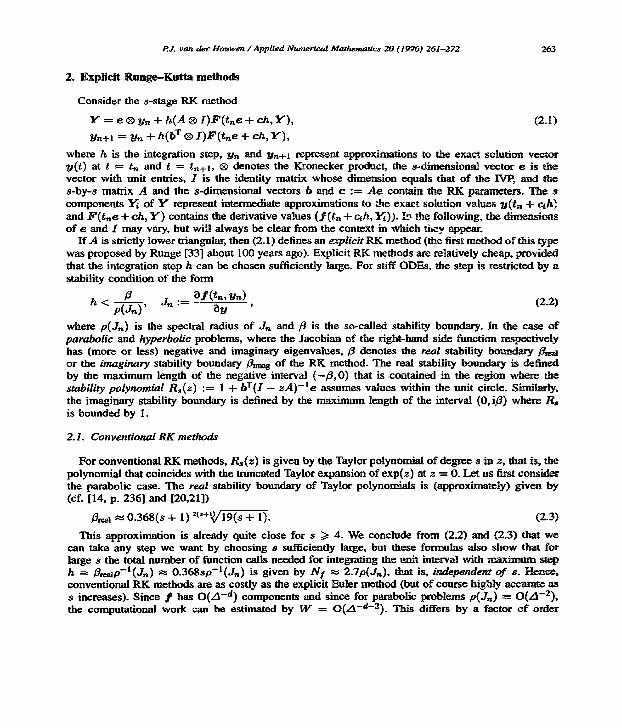
2. Explicit Runge--Kutta methods

Consider the s-stage RK method

Y = e ® Yn + h ( A ® I ) F ( t n e + ch, Y ) , (2.1)

Yn+l = Yn -t- h(b T ® I ) F ( t n e + ch, Y ) ,

where h is the integration step, ~/n and t/n+1 represent approximations to the exact solution vector y(t) at t ---- tn and t --- tn+l, ® denotes the Kronecker product, the s-dimensional vector e is the vector with unit entries, I is the identity matrix whose dimension equals that of the IN/P, and s-by-s matrix A and the s-dimensional vectors b and c :-- A e contain the RK paran~ters. The s components ~ of Y represent intermediate approximations to Lhe exact solution values ~ ( ~ + cih~ and F ( t n e + ch, Y ) contains the derivative values ( f ( t n + c~h, Yi)). ~ t~he following, the dhrtensions of e and I may vary, but will always be clear from the context in which they appear.

If A is strictly lower triangular, then (2.1) defines an explicit RK method (the first method of this type was proposed by Runge [33] about 100 years ago). Explicit RK methods are relatively cheap, provided that the integration step h can he chosen sufficiently large. For stiff ODEs, the step is restricted by a stability condition of the form

/3 0 f ( t n , Yn) (2.2) h < p ( j ~ ) , Jn : = a ~ '

where P(Jn) is the spectral radius of Jn and ~ is the so-called stability boundary. In the case of parabolic and hyperbolic problems, where the Jacobian of the right-hand side function respectively has (more or less) negative and imaginary eigenvalues, /3 denotes the real stability boundary or the imaginary stability boundary/~imag of the RK method. The real stability boundary is defined by the maximum length of the negative interval (--/3, 0) that is contained in the region where the stability polynomial Rs( z) :-" 1 + bT ( I -- z A ) - l e assumes values within the unit circle. Similarly, the imaginary stability boundary is defined by the maximum length of ~ e interval (0, ifl) where Rs is bounded by 1.

2.1. Conventional RK methods

For conventional RK methods, Rs(z ) is given by the Taylor polynomial o f degree s in z, that is, the polynomial that coincides with the truncated Taylor expansion of exp(z) at z -- 0. Let us first consider the parabolic case. The real stability boundary of Taylor polynomials is (approximately) given by (cf. [14, p. 236] and [20,21])

/~.al ~ 0.368(s + 1) 2c'+~)X/19(s + 1). (2.3)

This approximation is already quite close for s /> 4. We conclude from (2.2) and (2.3) that we can take any step we want by choosing s sufficiently large, but these formulas also show that for large s the total number of function calls needed for integrating the unit interval with maximum step h = ~ p - I ( J n ) ~ 0 .368sp- l (Jn) is given by N I ~ 2.7p(Jn), that is, independent o f s. Hence, conventional RK methods are as costly as the explicit Eulvr method (but of course highly accurate as s increases). Since f has O( / I -d) components and since for parabolic problems P(Jn) -- O(ZI-2), the computational work can be estimated by W -- O ( A - d - 2 ) . This differs by a factor of order

264 P..J. van der Houwen / Applied Numerical Mathematics 20 (1996) 261-272

O ( h A -3/2) from the estimate derived for the Crank-Nicolson, Laasonen and BDF2 methods (when applied to higher-dimensional problems). Usually, this factor is quite large (e.g., if h = O(A)) , so that conventional RK methods are not the way to solve space-discretized PDEs of parabolic type. They are "'too cosily and too accurate".

Next we consider the hyperbolic case. It happens that for the imaginary stability boundary/3imag we do not always obtain nonzero values. If z-O~+U[Rs(z) - exp(z)] --+ C'p+! as z ---* 0, where p denotes the order o f accuracy of the RK method, then it can straightforwardly been shown that/31mag is only nonzero if either C'p+li p < 0 for p even or C'r,+lir'+l < 0 for p odd. For the Taylor polynomials this implies that the imaginary stability interval is empty for p = 1, 2, 5, 6, 9, 10 . . . . . For the other orders, quite reasonable values are obtained. For example, for p = 3, 4, 7, 8, we have flimag ~ 1.7, 2.8, 1.7, 3.4. Taking one of these latter methods and assuming that p(dn) = O ( A - l ) , the total computational work associated with the unit interval can be estimated by W = O ( A - d - I ) . This is a factor o f order O ( h A - I / 2 ) better than the estimate derived for the Crank-Nicolson, Laasonen and BDF2 methods. Hence, unlike the situation for parabolic problems, conventional RK methods seem to be preferrable for hyperbolic problems.

2.2. Parabolic R K methods

Our conclusion that for parabolic problems explicit RK methods are "too costly and too accurate" suggests sacrifycing accuracy in order to reduce computational costs. By observing that an s-stage RK method of order p with s > p possesses a stability polynomial Rs of the form

1 2~s(P)(z) 2=/~0 + /~ lg +/~2 Z2 + . - . + /~sz s, /~ff = j--~, j = 0 , . . . ,p , (2.4)

where the coefficients /3j, j = p + 1 , . . . , s, are free parameters, it is natural to use these free parameters for obtaining larger stability boundaries. For parabolic problems, where the eigenvalues

of the Jacobian often are along the negative axis, we are led to construct polynomials R ~ ) (z) with

increased real stability boundary. Having found an appropriate stability polynomial Rs 0) , it is always possible to construct an RK method with R ~ ) as its stability polynomial (see, e.g., [14]). Such methods will be called parabolic RK methods.

Until now, closed form solutions for the polynomials with maximal real stability boundaries (to be called optimal polynomials) are only known for p = 1. They are given by the shifted Chebyshev polynomials

c ~ ) ( z ) := Ts 1 + ~ , t~,~ = 2s 2, (2.5)

where Ts(z) := cos(s arccos(z)) denotes the first kind Chebyshev polynomial of degree s. They have been rediscovered in the literature again and again (even in recent years, see, e.g., [2]). As far as I know, they were first mentioned for integrating parabolic equations: in 1958 by Yuan' Chzao-Din in his thesis [41], in 1959 by Franklin it: his paper [6] that appeared in the Journal o f Mathematical Physics, and in 1960 by Guillou and Lago in the proceedings [9] of the first conference of AFCAL (the French Association for Computing). These authors were not aware of each other 's work.

For p >1 2, only approximate solutions have been constructed. In the thesis of Metzger [28] in 1967, we find numerical approximations for p ~ 4, a <~ 5, and in a NASA report of Lomax [27] of 1968,

P.J. van der Houwen / Applied Numerical Mat]tematics 20 (1996) 261-272 265

a general approach for computing the coefficients was indicated. Lomax conjectured that the optimal polynomials satisfy the so-called equal ripple property, that is, the optimal polynomial has ~ - p local extrema +1 or - 1 (this property was actually proved by Riha [31] in 1972 Who also showed h'~e unique existence of the optimal polynomials for all p and all s > p). Using the equal ripple property, an iterative method can be constructed for the numerical computation of the coefficients. Ho~vever, this equal-ripple-iteration method needs rather accurate initial iterates in order to converge. Presumably for this reason, Lomax did not use the equal-ripple-property approach, anti instead, comgmted least squares approximations for p ---- 2 and 8 ~< 10. Again, Metzger, Lomax and Riha found the/r results independently.

At CWI we used the least squares approach of Lomax for generating initial i t c r a ~ to start the equal-ripple-iteration method. In this way, we computed the optimal stability polynomials, together with their real stability boundaries, t%-r p ~< 4 and s ~ 10 + p (tables for the coefficients can be found in [13,14]). These computations indicated that ~,~, increases quadratically with s as s increases. In fact, we found

~re~ ~ q'ps 2 as s -+ oo, "/2 = 0.814, "/3 = 0.489, q~4 = 0.341. (2.6)

The quadratic behaviour is important. R implies that the total number of function calls needed for in- tegrating the unit interval with maximum step h ~ %,s2p - ! (J,~) is now given by N f ~ (.yps)-lp(J,~), which is a factor 2.7"yps less than the number of function calls needed for conventional RK methods. Hence, for large values of s, RK methods generated by (2.5) are much cheaper than conventional RK methods, provided that they are available for large values of s. Unfortunately, the numerical compu- tation of the optimal polynomials becomes increasingly more difficuR as s increases. This motivated t~s to look for analytical expressions for nearly optimal polynomials that are valid for arbitrary high values of a. In 1971, Bakker [1] derived in his Master thesis for p ---- 2 and p ---- 3 analytically given polynomials which are quite close approximations to the optimal stability polynomials, in the sense that [he stability boundaries are close to the maximal attainable values. These polynomials, to be called the Bakker polynomials, are given by

Bs(2)(z) 2 s 2 + 1 8 2 - 1 _ ( 3z ) 2 = - - 3 - - ~ - - + ~ T s l+s--f-/~_l , / ~ : ~ . (a~ ' - - l ) , a > 2 , (2.7)

B ( s 3 ) ( z ) = l + 3 1 3 2 - 2 ( 4 0 k 2 - 1 ) ' - 576/¢4 3"2 -- 2(36k2 -- 1)flT2. ( l + - ~ ) 512k 4 (2.8)

+ 3 ~ 2 - 2 ( 4 k 2 - 1)/~Ts ( _ ~ ) s 4608k4 1 + , /c := ~, s ---- 6,12, 18 . . . . .

2 2 1~/8s4 - 6082 + 297 2 2 ( V ~ ) ~real~fl :----~s - - 1 + ~ 5 ~ s 1 + ~.0.36382 a s s - - + c o ,

where again Ts denotes the first kind Chebyshev polynomial of degree s (in addition, Bakker actually proved the quadratic behaviour of the real stability boundaries of the optimal polynomials and obtained lower and upper bounds for "y~, up to p = 15). A comparison of (2.6) with (2 .7)and (2.8) reveals that the Bakker polynomials respectively possess 80% and 75% of the maximal aRainabl¢, asymptotic stability boundary. Later on in 1982, we found for p = 2 an even bettor approximation given by (cf. [17])

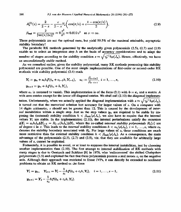
266 P.J. van tier Houwen I Applied Numerical Mathematics 20 (1996) 261-272

2 z z T " cos(It/s) + z (2.9) A~(2)(z) = 2 - z 2 -

2 s 2 /~real = [tan(Tr/2a)] 2 ~ 8~-~ ~ 0.810s 2 as s ~ oo.

These polynomials are not the optimal ones, but yield 99.5% of the maximal attainable, asymptotic stability boundary!

The parabolic RK methods generated by the analytically given polynomials (2.5), (2.7) and (2.9) enable us to select an integration step h on the basis of accuracy considerations and to adapt the

stages according to the stability condition s ~ ~ / ' t~ |hp (Jn ) . Hence, effectively, we have n u m b e r o f

an unconditionally stable method. As we remarked earlier, given the stability polynomial, many RK methods possessing this stability

pol~;nomial are possible. One of the most simple implementations of first-order or second-order RK methods with stability polynomial (2.4) reads

1"~ = y, , + aihJ ' ( t~ + c a - l h , ~ - l ) ,

Yn+l = yn + h f ( t ~ + h, Ys) ,

~ s - - i + 2 , . . . ai := ~s- i+l i = 1, , s , (2.10)

where al is assumed to vanish. This implementation is of the form (2.1) with b = es and a matrix A with zero entries except for the lower off-diagonal entries. We shall cal! (2.10) the diagonal implemen-

Unfortunately, when we actually applied the diagonal implementation with s ~ ~ / 7 ~ l h p ( J n ) , ration.

it tumod out that the numerical solution lost accuracy for larger values of s. On a computer with 14 digits arithmetic, s should not be greater than 12. This is caused by the development of inter- hal instabilities within a single step. Just as the step values Sin are required to be stable by im- posing the (extemal) stability condition h < Breal/P(Jn), we also have to require that the internal values I,~ are stable. In the implementation (2.10), the internal perturbations satisfy the recursion AYi = a~hJnAY~- l = Pq- l ( hJn )AYl , where the so-called internal stability polynomials Pq ( z) are of degree i in z. This leads to the internal stability conditions h < c~i/p(Jn), i = 1 , . . . , s, where oq denotes the stability boundary associated with R/. For large values of s, these conditions are much more restrictive than the external stability condition h < ~real/P(Jn). As a consequence, the main advantage of the polynomials (2.5), (2.7) and (2.9), viz. that they are available for arbitrarily large values of s, cannot be exploited.

Fortunately, it is possible to avoid, or at least to suppress the internal instabilities, just by choosing another implementation than (2.10). The first attempt to internal stabilization of RK methods with many stages is due to G-entzsch and SchRRer [8] in 1978, who 'rediscovered" the shifted Chebyshev polynomials (2.5) and exploited the fact that these polynomials possess s real zeroes zi on the negative axis. Although their approach was restricted to linear IVPs, it can directly be extended to nonlinear problems to. obtain an RK method o~ the form

| _ YI ~- Yn, Yi+l = ~ -- - - h f ( t n "t" cah, ~ ) ,

zi

Zs

i = 1 , . . . , s - 1, (2.11)

P.J. van der Houwen / Applied Numerical MatY~ematics 20 (1996) 261-272 267

This implementat ion may be interpreted as an RK method that is factorized in a sequence of Euler steps and will be called the fac tor i zed implementation. If the zeroes zi are ordered such that z~ < z~+l or zi > zi+i, then the performance the factorized irrtplementation is hardly better than that of the diagonal implementat ion as s increases. However, Gentzsch and Schlfiter r e p o ~ satisfactory results for extremely large values o f s (up to 997) if special orderings o f the z~ are used. A disadvantage in actual applications is that a suitable ordering depends on s.

When reading the paper of Gentzsch and Schl~ter, we suddenly realized that the problem o f in|ernal stabilization was already solved a long time ago by numerical analysts working in eltipffc PDEs! The spatial discretization of elliptic PDEs leads to the problem of solving linear systems A y = b, where A is known to have a negative spectrum in the negative interval ( - - p ( A ) , 0) with p ( A ) large positive. A well-known iterative method for solving such problems is due to Richardson, who proposed in his paper [30] o f 1910 the recursion ~ = Y~-l + ~ i ( A y i - ! -- b) , where the parameters o~ are chosen such that after s iterations, the polynomial Ps occurring in the error formula Y8 -- Y = P i (A) (yo -- y ) has a small norm in the eigenvalue interval (a, b) of A. Various approaches to achieve this have been prol~osed. Richardson suggested choosing Ps such that it has uniformly distributed zeros in (a, b), Stiefel proposed to minimize an integral measure of P8 (cf. [36]), but most numerical analysts prefer to minimize the m a x i m u m norm of Ps. The latter approach leads to shifted Chebyshev polynomials that are very similar to (2.5). This process is now known as Richardson's method o f f i rs t degree. However, application of this method for large values of s suffers the same internal instability as the method (2.11). Just as Gentzsch and Schlfiter, one has tried to improve the stability by special choices of the ordering of the parameters a~ (see, e.g., the experiments o f Young [40] in 1954), but a real break-through was due to Stiefel [36] in 1958. He observed that Chebyshev polynomials satisfy a stable three-term recursion, so that using a three-term recursion for the iterates Yi, r a t e r than the two- term recursion of Richardson, would avoid the instability problem. This two-step iteration method is known as Richardson's method of second degree or, in the more recent literature, the Chebyshev semi- iterative method . Realizing that the stability polynomials (2.5), (2.7) and (2.9) are also expressions in terms of shifted Chebyshev polynomials, brought us to construct internally stable implementat ions o f the corresponding parabolic RK methods (cf. [15,16]). For the second-order consistent polynomials A(~ 2) and B~ (2), it was pointed out by Sommei jer (see [15]) that it is even possible to make the Y~ not only stable, but Aso second-order accurate approximations to the exact solution at the intermediate points tn + c~h, i = 1 . . . . , s .

The internally stable Runge-Kut ta method generated by the Bakker polynomials B (2) performs slightly better than the method generated by A(~ 2) (its smaller stability boundary is c o m p e n ~ ' ~ d by its smaller error constants). It is a highly efficient integrator for general heat flow problems, p~rticularly for 2D and 3D problems. We called it the R u n g e - K u t t a - C h e b y s h e v method, but is could equally well have been called the R u n g e - K u t t a - B a k k e r method. A detailed study of its convergence is presented in [37] and an extensive performance evaluation can be found in [12]. The R u n g e - K u ~ b y s h c v method has been implemented by Sommeijer as the code RKC and is available through netlib [34].

Another code that is based on stabilized RK methods is the code DUMKA developed by Lebedev and his coworkers of the Institute for Numerical Mathematics o f the Russian Academy of Science. They approximate the optimal stability polynomials by so-called Zolotarev polynomials. Like Gentzsch and SchlUter, internal stability is achieved by a special ordering of the stages rather than using recurrence relations. More details can be found in the references [25,26].

268 P..j. van tier Houwen I Applied Numerical Mathematics 20 (1996) 261-272

Finally, we compare the total computational work of conventional and parabolic RK methods needed for integrating the unit interval with a given step h. Assuming that s is defined by

s ~ ~ / ' r ;~ho (Jn ) , we find for the stabilized RK methods

w = h-'~ o(z~-~) ~ h-' X/~;'hp(&) o(~ -~) ~ o(~-'/: ~-~-'). Comparing this estimate with that derived for conventional RK methods, we see that the computa~onal complexity of the stabilized RK methods differ by a factor of order O(ht/2Z~-l). With respect to the Crank-Nicolson, Laasonen and BDF2 methods using conjugate gradient type iteration methods, the stabilized RK methods are at least competitive.

2.3. Hyperbolic RK methods

Instead of maximizing the real stability boundary of stability polynomials of the form (2.4), we may also maximize the imaginary stability boundary, to obtain a hyperbolic RK method that should be suitable for integrating hyperbolic problems that have Jacobians with imaginary eigenvalues.

For p = 1, the optimal polynomials are given by

z 2 I ( , ) ( z ) = ( _ i ) s [ i T s _ , ( s i Z _ l ) _ ( l + ____~)2) U [" iz • (~ ._2 \ 7 : - ~ ] ] , (2.12) 3~ag = s - 1 , s >/ 2,

where Us(Z) := sin((s + 1)arccos(z))/sin(arccos(z)) denotes the second kind Chebyshev polynomial of degre~ z. For odd values of s, these polynomials were given in 1972 in [13] (a proof can be found in [14]). At the time, it was not realized that (2.12) is also valid for even values of s, because in [13] the polynomials I (1) were represented in the form

z 2

f l i n g = s - I , s - - 2 k + l , k / > l ,

which cannot directly be extended to even values of s. It tams out that the odd-degree polynomials are identical to the optimal polynomials corresponding m p = 2, i.e., I(82)(z) = I~l)(z) for s odd.

In 1984 Kinnmark and Gray [22] derived the representation (2.12) which is valid for all values of s. This result was also obtained, independently, by Sonneveld and van Leer [35] in 1985.

Kinnmark and C.nay [23] have also derived approximations to the optimal polynomials I~ (3) for s odd and to I8 (4) for s even. These Kinnmark--Gray polynomials are given by

' [ K~(3)(z) = ~ - ~ l + z + i8-1~2Ta_1

+ l i s + 2 t ~ { ( s - 2 ) T , ( f l ) - sT,-2 ( ~ ) } ] , (2.14)

/ ~ = / ~ : = V / ( s - 1 ) 2 - 1 , o d d s > t 3 ,

P.J. van der HotoNen / Applied Numerical Mathematics 20 (1996) 261-272 269

and

i I [is+I/~Ts-i (~) + li'{(s - 2)Ts (~) -- sTs_2 (~) ~], (2.15) K p ) f z ) =

~img = f~ : = ~ / ( s - l ) 2 - 1, e v e n s / > 4 .

Earlier, in 1983, Vichnevetsky [38] had already proved that ~ ~ s -- l for all p and s. H e ~ , result of Vichnevetsky indicates that the Kinnmark--Gray polynomials are exUemely close approxima- tions to the optimal ones. However, it also indicates that, unlike the situation for parabolic problems, hyperbolic RK methods are hardly more effective than conventional RK methods with nonempty imagin~y stability intervals.

3. Spli t t ing me thods

Just as RK methods, splitting methods compute in each step two or more intermediate stages. However, unlike RK methods, these stages are not expressed in the full right-hand side of the PDE, but in fractions of the right-hand side. Almost all splitting methods proposed in the literatme can be represented in RK format. This approach was followed in [19] to develop a unified treatment of splitting methods and allows a straightforward derivation of the order conditions and stability functions.

Suppose that the right-hand side function in (1.1) is split according to

:ff, y(t)) = ~ f~ff, y(t)), (3.1) i=1

and consider the RK type method

Y = e ® Yn + h ~ (A (k) ® I )Fk ( tne + c(k)h, Y ) , (3.2) k = i

Yn+i = ( e T ® I)Y, where Fk(tne + c ( k ) h , Y ) contains the derivative values ( :k ( tn + c~P)h,]~)). If ~r = 1, then (3.2) reduces to the RK method (2.1) with b T = eTA. The method {(3.1), (3.2)} will be called a ~-term RKS method with s fractional stages. RKS methods consist of two components, the right-hand side splitting (3.1) and the splitting scheme (3.2).

Restricting our discussion to first-order and second-order methods and using the compact notation in terms of the matrices A(k), we have first-order accuracy if

eTA0)e---- 1, j ---- l , . . . , c r , (3.3)

and second-order accuracy if. in addition,

1 j , k f l , ,o-. (3 .4 ) eTAO)A(k)e = ~, "..

In principle, the abscissa vectors are defined by c (k) := A(~)e. However, in actual computations, the time-dependent parts originating from time-dependent boundary conditions, need a more careful treatment. In this overview, we shall not elaborate on this aspect of splitting methods (see, e.g., [5]).

270 P.& van tier Houwen /App l i ed Nuraerical Mathematics 20 (1996) 261-272

The linear stability of RKS methods can be analysed by means of the linear test equation

~'(0 - ~ Jky(O, (3.5) k-----!

where J~ is the Jacobian matrix Ofk(yn)/dy. It will be assumed that Jk has its eigenvalues in the left halfplane. DefinKng Zk = hJk, k -- 1 , . . . , ~r, we deduce from (3.2)

• Y = e ® y n + ~ ( A ( k ) ® Z k ) Y = ( I - S ) - l ( e ® y n ) , S : = ~ ( A ( k ) e Z k ) . k----I k----!

H e n c e ,

Thus, the stability function is given by

( ) R = (e T ® I ) ( I ® I ) - (A (t~) ® Zt~) (e ® I) . (3.6) k----I

3.1. Splitting methods as RKS methods

This survey paper is concluded with an example of a family of splitting methods that can be represented as an RKS method. For a more 4 e . ~ e d analysis of RKS methods with an application to transport problems in three spatial dimensions, we refer to [18].

Consider the two-term, three-stage splitting scheme defined by

A (n )= ½ 0 , A {2)= 0 ½ • (3.7)

0 0 1

This scheme is second-order accurate whatever we choose for f l and J~2- Presumably, the first splitting method proposed in the literature generated by the splitting scheme (3.7) is the Peaeeman-Raehford method [29] of 1955. If (3.7) is applied to a space-discretized, two-dimensional PDE in which the right-hand side f can be split into an x-dependent part .fl and a y-dependent part ,f2, then the so-called ADI (Alternating Dire~etion Implicit) method of Pea®®man and Raehford is obtained. Other well-known splitting methods generated by (3.7) are the Hopscotch methods proposed by Gourlay in 1970. These methods are obtained by dividing the grid points on which the PDE is discretized in two groups G1 and G2, and by defining f l and f2 such that they vanish on Gl and G2, respectively. On rectangular grids, often used examples are the Line Hopscotch and the Odd-Even Hopscotch methods which arise if Gl and G2 contain grid points lying on alternating lines and diagonals, respectively.

A c k J o ~ e m e n t

The author is grateful to Dr. B.P. Sommeijer for his interest in this survey paper and for his many comments to improve the presentation of the available material.

p.J. van ¢ler Houwen / Applied Numerical Mathematics 20 (1996) 261-272 271

References

[ 1 ] M. Bakker, Analytic aspects of a minimax problem, Report "IN 62, Mathematisch Cenmm~ (1971) (in Dutch).

[2] K. Burrage, Order and stability properties of explicit multi-¢alue methods, Appl. Numer. Ma~. I (1985) 363-379.

[3] C.E Curtiss and J.O. Hhschfelder, Integration of stiff equations, Proc. Nat. Acad. ScL U.S. 38 (1952) 235-243.

[4] J. Crank and P. Nicolson, A practical method for numerical integration of solutions of ~ ~ e r e n ~ l equations of heat-conduction type, Proc. Cambridge Philos. Sac. 43 (1947) 50-67.

[5] G. Fairweather and A.R. Mitchell, A new computational procedure for A.D.L methods, SIAM J. Num~r. Anal 4 (1967) 163-170.

[6] J.N. Franklin, Numerical stability in digital and analogue computation for diffusion problems, J. Math. Phys. 37 (1959) 305-315.

[7] C.W. Gear, Numerical Initial Value Problems in Ordinary Differential Equations (Prentice Hall, Englewood Cliffs, NJ, 1971).

[8] W. Gentzsch and A. Schliiter, On one-step methods with cyclic stepsize changes for solving tmrabolic differential equations, Z Angew. Math. Mech. 58 (1978) T415-T416 (in German).

[9] A. Guillou and B. Lago, Stability regions of oue-step and multistep formulas for differential equations: investigation of formulas with large stability boundaries, 1 e Congres de l'Association Franeai__se de C a l c ~ AFCAL, Grenoble (1960) 43-56 (in French). E. Hnirer, S.P. Nersett and G. Wanner, Solving Ordinary D~fferential Equations, I: N ~ Problems (Springer, Berlin, 1987/91). P. Henrici, Discrete Variable Methods in Ordinary Differential Equations (Wiley, New York, 1962). S. Hofmann, First and second-order Runge-KuRa-Chebyshev methods for the nmnerical imegrath~ of parabolic differential equations and stiff ordinary differential equations, Master's ~ s , U n i v e m ~ of Wuppertal, Germany (1992) (in German). P.J. van der Houwen, Explicit Runge--Kutta methods with increased stability boundaries, Numer. Math. 20 (1972) 149-164. P.J. van der Houwen, Construction of Integration Formulas for Initial-Value Problems (North-HoUaad, Amsterdam, 1977). P.J. van der Houwen, On the time integration of parabolic differential equations, in: G.A. Watson, ed., Numerical Analyais, Lecture Notes in Mathematics 912 (Springer, New York, 1981) 157-168. PJ. van der Houwen and B.P. Sommeijer, On the internal stability of explicit m-stage Runge--Kutta methods for large values of m, Z Angew. Math. Mech. 60 (1980) 479--485. PJ. van der Houwen and B.P. Sommeijer, A special class of multistep Runge--KuRa methods with exmmk~ real stability interval, IMA J. Numer. Anal. 2 (1982) 183-209. P.J. van der Houwen and B.P. Sommeijer, Splitting methods for three-dimensional trrmsport models with interaction terms, J. Scientific Comput. (submitted). PJ. van der Houwen and J.G. Verwer, One-stop splitting methods for semidiscreto peaaboli¢ Computing 22 (1979) 291-309. R. Jeltsch and O. Nevanlinna, Stability and accuracy of time discretizafions for initial value Report HTKK-MAT-A 187, Helsinki University of Technology ( 1981 ). P. Jeltsch and O. Nevanlinna, Stability of explicit time discretizations for solving initial value Numer. Math. 37 (1981) 61-91. LEE. Kinnmark and W.G. Gray, One-step integration methods with maximum stability r e ~ , Math. Comput. Simulation 16 (1984) 87-92.

[lO]

[11] [12]

[131

[14]

D5]

[16]

[17]

[18]

[19]

[2o]

[21]

[22]

272 P.J. van der Houwen / Applied Numerical Mathematics 20 (1996) 261-272

[23] LP.E. Kinnmark mid W.G. Gray, One-step integration methods of third-fourth order accuracy with large hyperbolic stability limRs, Math. Comput. Simulation 16 (I984) 181-I 84.

[24] P. Laasonen, On a meglod for solving the heat flow equation, Acta Math. 81 (1949) 309-323 (in German). [25] V.L. Lebedev, Explicit difference schemes with time-variable steps for solving stiff systems of equations,

Preprint No. 177, Dept. of Numerical Mathematics, USSR Acad. Sc., Moscow (1987) (in Russian). [26] V.L. Lebedev, How to solve stiff systems of equations by explicit difference schemes, in: G.I. Marchuk,

od., Nume~cal Methods and Applications (CRC Press, Ann Arbor, MI, 1994) 45-80. [27] H. Lomax, On the construction of highly stable, explicit numerical methods for integrating coupled ODEs

with parasitic eigenvalues, NASA Technical Note NASAIN D/4547 (1968). [28] C.L. Metzger, Runge-Kutta methods whose number of stages exceeds their order, These (Troisieme cycle),

Universit6 do Grenoble (1967) (in French). [29] D.W. Peaceman and H.H. Rachford Jr, The numerical solution of parabolic and elliptic differential equations,

J. Soc. lndust. Appl. Math. 3 (1955) 28-41. [30] L.F. Richardson, The approximate arithmetical solution by finite differences of physical problems involving

differential equations, with an application to the stresses in a masonry dam, Philos. Trans. Roy. Soc. London Set. A 210 (1910) 307-357 and Prec. Roy. Soc. London Ser. A 83 (1910) 335-336.

[31] W. Riha, Optimal stability polynomials, Computing 9 (1972) 37-43. [32] E. Rothe, Two-dimensional parabolic boundary value problems as limiting case of one-dimensional boundary

value problems, Math. Ann. 102 (1930) 650-670 (in German). [33] C. Runge, Oil the numerical solution of differential equations, Math. Ann. 46 (1895) 167-178 (in German). [34] B.P. Sommeijer, RKC, a nearly-stiff ODE solver, available through netlib (mail: netlib@ornl.gov, send rkc.f

from ode) (1991). [35] P. Sonneveld and B. van Leer, A minimax problem along the imaginary axis, Nieuw Archiefvoor Wiskunde

3 (4) (1985) 19-22. [36] E.L. Stiefel, Kernel polynomials in linear algebra and their numerical applications, Nat. Bur. Stand. Appl.

Math- Series 49 (1958) 1-22. [37] J.G. Verwer, W.H. Hundsdorfer and B.P. Sommeijer, Convergence properties of the Runge-Kutta--Chebyshev

method, Numer. Math. 57 (1990) 157-178. [38] R. Vichnevetsky, New stability theorems concerning one-step numerical methods for ordinary differential

equations, Math. Comput. Simulation 25 (1983) 199-205. [39] N.N. Yanenko, The Method o f Fractional Steps (Sprit~ger, Berlin, 1971). [40] D.M. Young, On Riehardson's method for solving linear systems with positive definite matrices, J. Math.

Phys. 32 (1954) 243-255. [41] Yuan" Chzao-Din, Some difference schemes for the solution of the first boundary value problem for linear

differential equations with partial derivatives, Thesis, Moscow State University (1958) (in Russian).