UNIVERSITI UTARA MALAYSIA BPMN 6053 MANAGEMENT INFORMATION SYSTEM

The Development of Low-Order Models for the Study ofFluid-Structure Interactions
Thesis by
Andrew A. Tchieu
In Partial Fulfillment of the Requirements
for the Degree of
Doctor of Philosophy
California Institute of Technology
Pasadena, California
2010
(Defended September 3, 2010)

ii
c© 2010
Andrew A. Tchieu
All Rights Reserved

iii
Acknowledgments
First and foremost, I would like to thank my advisor, Professor Anthony Leonard. He is a beacon
of kindness, has always been very supportive through all my endeavors, and genuinely cares for my
overall wellbeing. I can say without any doubt that his guidance and encouragement helped me
through many difficult times during my life. For that I am immensely indebted to him. It has been
an honor to be his student and a part of him will forever be instilled in me.
I would also like to express gratitude to my thesis committee members, Professors Beverley
McKeon, Tim Colonius, and Dale Pullin. I have had the pleasure to take courses from each one of
them and all have had an important part in my academic development.
I also want to thank several Professors associated with Caltech. Professor John Dabiri has been
inspiring and has taken the time to play on the Aero basketball team together with me among
other things. Professors Hans Hornung and Joe Shepherd have always been very interactive with
the members of our lab, constantly checking in to see how we are doing. In particular, I have
had the privilege to play tennis with a great tennis player in Professor Hornung, who consistently
outdueled me. Undoubtedly, he would have been a great tennis player if someone had not convinced
him to study fluid mechanics. Thanks to Professor Darren Crowdy who gave me several ideas that
contributed to the fourth chapter of this thesis. His enthusiasm for teaching has been contagious
and I hope one day to replicate his passion in the classroom.
I am also grateful to have interacted with all members of the Iris and Puckett Laboratories. In
particular, I met Hans Jonas as a visiting student in our lab, and he has been a great friend over
the past few years.
My friends have been an unimaginably important part of my life. Perhaps the closest friends I

iv
have and definitely the most influential during my experiences here at Caltech are my roommates.
We have all shared many the same experiences and thoughts that have shaped my Ph.D. experience.
Won Tae Joe and I come from the same background and had many profound conversations about
school and life in this perspective. Jeff Hanna has been the person that I possibly spend the most
time with here at Caltech, whether it be eating a lot of good food, drinking beer, or doing outdoor
activities (mainly running or biking). Emily McDowell has been a very good friend and I cherish
the dinners we have had talking about various things, both important and inconsequential. Dominic
Rizzo has been a constant source of humor and entertainment. Thanks to all my other friends at
Caltech, especially John Meier and Chris Kovalchick who I have had the pleasure of interacting with
on and off campus, whether it be biking or just having a meal. I would also like to thank Francis
Castillo and Kent Chau, who are two of my best friends from high school, for their support and
friendship. You are all good friends and have shaped me to be who I am today, and I thank you
from the bottom of my heart for being in my life.
I would also like to thank my girlfriend and best friend of all, Nancy Diep. I am the luckiest
man in the world to have found my soul mate. She has been exceptionally supportive through all
my mood swings while researching and writing my thesis. I will do everything in my power to make
you the happiest woman in the world.
Last, but not least, I would like to thank my mom, dad, brother, and sister. They, above all,
have been the most supportive throughout my whole education. When the times were rough, they
were the ones constantly listening and comforting me while I was complaining and being dramatic.
With their unconditional love and support, I was able to complete my Ph.D. degree. I love you all.

v
Abstract
In this work, several low-order models are derived to describe and simulate fluid-structure interaction
problems with rigid bodies at a modest computational cost. The models are based on the inviscid
flow assumption such that potential theory can be used with, in some cases, point vortices in the
flow. Three general areas of application are considered. First, a thin airfoil undergoing small-scale
unsteady motions in the presence of a freestream flow is investigated. The low-order model that is
developed has only one ordinary differential equation for the fluid dynamic variables. This model is
used to briefly investigate vortex-induced flutter in the attached-flow regime and control of a free-
flying airfoil using synthetic jet actuators. Second, the vortex-induced vibrations of an arbitrary
bluff body in the presence of vortices, with or without a freestream flow, are considered. Several
examples of the canonical mass-spring-damper system for a circular cylinder and a flat plate are
given to demonstrate the use of the vortex-based model for these applications. Finally, the two-
body problem in a potential flow is addressed. A relatively simple solution specific to the doubly
connected domain is determined and its resulting force and moment are coupled to the rigid bodies
to investigate the mutual interactions between the two bodies. Aspects of drafting behind a forced
body, the role of the fluid in elastic collision, and flapping flight are discussed in this context.
Although a few specific examples and applications are given for each chapter, the main purpose of
the thesis is to present low-order potential flow methods that are applicable to a variety of situations.

vi

vii
Contents
1 Introduction 1
1.1 Motivation and background . . . . . . . . . . . . . . . . . . . . . . . . . . . . . . . . 1
1.2 Thesis outline . . . . . . . . . . . . . . . . . . . . . . . . . . . . . . . . . . . . . . . . 7
2 A simple discrete-vortex model for the non-uniform motion and control of a thin
airfoil 9
2.1 Introduction . . . . . . . . . . . . . . . . . . . . . . . . . . . . . . . . . . . . . . . . . 9
2.2 Aerodynamic model formulation . . . . . . . . . . . . . . . . . . . . . . . . . . . . . 11
2.2.1 Assumptions . . . . . . . . . . . . . . . . . . . . . . . . . . . . . . . . . . . . 12
2.2.2 Bound vortex circulation . . . . . . . . . . . . . . . . . . . . . . . . . . . . . 14
2.2.3 Quasi-steady bound circulation . . . . . . . . . . . . . . . . . . . . . . . . . . 16
2.2.4 Wake vortex dynamics . . . . . . . . . . . . . . . . . . . . . . . . . . . . . . . 17
2.2.5 Aerodynamic lift and moment . . . . . . . . . . . . . . . . . . . . . . . . . . . 19
2.2.6 Integration in time . . . . . . . . . . . . . . . . . . . . . . . . . . . . . . . . . 22
2.2.7 Quasi-steady camber and thickness corrections . . . . . . . . . . . . . . . . . 23
2.2.8 Summary of the low-order model . . . . . . . . . . . . . . . . . . . . . . . . . 24
2.3 Validation of the low-order model . . . . . . . . . . . . . . . . . . . . . . . . . . . . . 25
2.3.1 Comparison with experiments . . . . . . . . . . . . . . . . . . . . . . . . . . . 25
2.3.2 Comparison with delayed detached-eddy numerical simulatons . . . . . . . . 28
2.4 Vortex-induced flutter of a simple two degree of freedom system . . . . . . . . . . . . 30
2.5 Control of a two-dimensional airfoil . . . . . . . . . . . . . . . . . . . . . . . . . . . . 35

viii
2.5.1 Setup . . . . . . . . . . . . . . . . . . . . . . . . . . . . . . . . . . . . . . . . 35
2.5.2 Modeling ZMF synthetic jet actuators . . . . . . . . . . . . . . . . . . . . . . 36
2.5.3 Static fitting for the shift in Kutta condition and trapped vortex strength . . 40
2.5.4 Comparison between experiments . . . . . . . . . . . . . . . . . . . . . . . . . 42
2.5.5 Simple feedback for reduction of vortex induced oscillations . . . . . . . . . . 43
2.6 Conclusions . . . . . . . . . . . . . . . . . . . . . . . . . . . . . . . . . . . . . . . . . 44
3 An inviscid low-order model for the vortex-induced vibration of bluff bodies 47
3.1 Introduction . . . . . . . . . . . . . . . . . . . . . . . . . . . . . . . . . . . . . . . . . 47
3.2 General formulation . . . . . . . . . . . . . . . . . . . . . . . . . . . . . . . . . . . . 50
3.2.1 Conformal map . . . . . . . . . . . . . . . . . . . . . . . . . . . . . . . . . . . 50
3.2.2 Boundary conditions and associated potentials . . . . . . . . . . . . . . . . . 50
3.2.3 Definition of the velocity . . . . . . . . . . . . . . . . . . . . . . . . . . . . . . 52
3.2.4 Equation of motion for vortices . . . . . . . . . . . . . . . . . . . . . . . . . . 53
3.2.5 Force . . . . . . . . . . . . . . . . . . . . . . . . . . . . . . . . . . . . . . . . 54
3.2.6 Torque . . . . . . . . . . . . . . . . . . . . . . . . . . . . . . . . . . . . . . . . 56
3.2.7 Coupled equations of motion . . . . . . . . . . . . . . . . . . . . . . . . . . . 57
3.3 Vortex-induced vibrations of a circular cylinder . . . . . . . . . . . . . . . . . . . . . 57
3.3.1 Equations of motion . . . . . . . . . . . . . . . . . . . . . . . . . . . . . . . . 58
3.3.2 Results . . . . . . . . . . . . . . . . . . . . . . . . . . . . . . . . . . . . . . . 60
3.4 Vortex-induced vibration of a flat plate at high angles of attack . . . . . . . . . . . . 65
3.4.1 Equations of motion . . . . . . . . . . . . . . . . . . . . . . . . . . . . . . . . 66
3.4.2 Separation model and the Kutta condition . . . . . . . . . . . . . . . . . . . . 67
3.4.3 Results . . . . . . . . . . . . . . . . . . . . . . . . . . . . . . . . . . . . . . . 71
3.5 Conclusion . . . . . . . . . . . . . . . . . . . . . . . . . . . . . . . . . . . . . . . . . 73
4 Fluid-structure interactions of two bodies in an inviscid fluid 75
4.1 Introduction . . . . . . . . . . . . . . . . . . . . . . . . . . . . . . . . . . . . . . . . . 75

ix
4.2 Potential flow formulation . . . . . . . . . . . . . . . . . . . . . . . . . . . . . . . . . 77
4.2.1 Formulation of the boundary value problem . . . . . . . . . . . . . . . . . . . 77
4.2.2 Analytic solution to the boundary value problem . . . . . . . . . . . . . . . . 80
4.3 Hydrodynamic coupling . . . . . . . . . . . . . . . . . . . . . . . . . . . . . . . . . . 83
4.3.1 Hydrodynamic forces and moment . . . . . . . . . . . . . . . . . . . . . . . . 83
4.3.2 Coupled fluid-structure interactions . . . . . . . . . . . . . . . . . . . . . . . 85
4.4 Two interacting circular cylinders . . . . . . . . . . . . . . . . . . . . . . . . . . . . . 85
4.4.1 Conformal map . . . . . . . . . . . . . . . . . . . . . . . . . . . . . . . . . . . 86
4.4.2 Complex potential solution . . . . . . . . . . . . . . . . . . . . . . . . . . . . 86
4.4.3 Forces induced from inline impact of two circular cylinders . . . . . . . . . . 87
4.4.4 Coupled dynamics of two circular cylinders . . . . . . . . . . . . . . . . . . . 90
4.5 A pair of flapping parallel plates . . . . . . . . . . . . . . . . . . . . . . . . . . . . . 99
4.5.1 Conformal map . . . . . . . . . . . . . . . . . . . . . . . . . . . . . . . . . . . 99
4.5.2 Sinusoidal flapping and pitching . . . . . . . . . . . . . . . . . . . . . . . . . 100
4.6 Conclusion . . . . . . . . . . . . . . . . . . . . . . . . . . . . . . . . . . . . . . . . . 103
5 Conclusion and future directions 107
5.1 Conclusions . . . . . . . . . . . . . . . . . . . . . . . . . . . . . . . . . . . . . . . . . 107
5.2 Future directions . . . . . . . . . . . . . . . . . . . . . . . . . . . . . . . . . . . . . . 109
Appendix A Simulink models of the experimental apparatus 111
Appendix B Vortex model based adaptive flight control using synthetic jets 113
B.1 Introduction . . . . . . . . . . . . . . . . . . . . . . . . . . . . . . . . . . . . . . . . . 113
B.2 Control formulation . . . . . . . . . . . . . . . . . . . . . . . . . . . . . . . . . . . . 116
B.2.1 A simplified control design model . . . . . . . . . . . . . . . . . . . . . . . . . 116
B.2.2 Linear control algorithm . . . . . . . . . . . . . . . . . . . . . . . . . . . . . . 118
B.2.3 Augmenting output feedback adaptive control . . . . . . . . . . . . . . . . . . 122
B.2.4 Control hedging . . . . . . . . . . . . . . . . . . . . . . . . . . . . . . . . . . 126

x
B.3 Model and control design validation . . . . . . . . . . . . . . . . . . . . . . . . . . . 127
B.3.1 Regulating control vortex strength . . . . . . . . . . . . . . . . . . . . . . . . 127
B.3.2 Experimental results . . . . . . . . . . . . . . . . . . . . . . . . . . . . . . . . 128
B.4 Conclusion . . . . . . . . . . . . . . . . . . . . . . . . . . . . . . . . . . . . . . . . . 131
Appendix C Example translation and rotation potentials 135
Appendix D Details on integrating the two body FSI problem 139

xi
List of Figures
2.1 Schematic of the unsteady vortex dynamics model . . . . . . . . . . . . . . . . . . . . 11
2.2 Schematic of the quasi one-dimensional simplification . . . . . . . . . . . . . . . . . . 12
2.3 Summary of the low-order model . . . . . . . . . . . . . . . . . . . . . . . . . . . . . . 24
2.4 Schematics of the NACA 4415 airfoil model and its free-flight test bed . . . . . . . . . 25
2.5 Comparison with experimental results for pure pitching . . . . . . . . . . . . . . . . . 27
2.6 Comparison with numerical simulations in pure pitch . . . . . . . . . . . . . . . . . . 28
2.7 Vorticity field from DDES simulation demonstrating small-scale vortices shed off the
non-sharp trailing edge (Lopez, 2009). . . . . . . . . . . . . . . . . . . . . . . . . . . . 29
2.8 Comparison with numerical simulations in pure plunge . . . . . . . . . . . . . . . . . 30
2.9 Schematic for the vortex-induced flutter of a flat plate airfoil . . . . . . . . . . . . . . 31
2.10 Various simulations of vortex-induced fluttering . . . . . . . . . . . . . . . . . . . . . . 33
2.11 Case (e), a multi-modal response of a fluttering airfoil . . . . . . . . . . . . . . . . . . 34
2.12 FFT of the response in Figure 2.11 plotted versus non-dimensional frequency . . . . . 35
2.13 Normalized vorticity plots of synthetic jets over a modified airfoil . . . . . . . . . . . . 37
2.14 Numerical and theoretical evidence for shift in Kutta condition . . . . . . . . . . . . . 38
2.15 Change in lift versus change in moment due to control . . . . . . . . . . . . . . . . . . 40
2.16 Relationship between ΓC, uC, and α . . . . . . . . . . . . . . . . . . . . . . . . . . . . 41
2.17 Comparison of test bed simulation with experimental results . . . . . . . . . . . . . . 42
2.18 Simple feedback is used to reduce induced vibrations . . . . . . . . . . . . . . . . . . . 44
3.1 Schematic of a body interacting with N point vortices in the physical-plane and the
mapped-plane . . . . . . . . . . . . . . . . . . . . . . . . . . . . . . . . . . . . . . . . 49

xii
3.2 Schematic of the application of Cauchy’s theorem to deform ∂D0 . . . . . . . . . . . . 55
3.3 Schematic of the vortex-induced vibration for a circular cylinder in cross flow . . . . . 58
3.4 Response of the system for z1(t = 0)/D = 0.930 with kz = 1 and bz = 0 at t = 500 . . 61
3.5 Maximum amplitude versus vortex separation distance, z1/D . . . . . . . . . . . . . . 62
3.6 Response of the system for z1(t = 0)/D = 1.275 and z2(t = 0)/D = 1.275i with kz = 1
and bz = 0 at t = 100 . . . . . . . . . . . . . . . . . . . . . . . . . . . . . . . . . . . . 63
3.7 Schematic defining the parameters in the vortex street . . . . . . . . . . . . . . . . . . 63
3.8 Max displacement versus Strouhal frequency of incoming vortex street . . . . . . . . . 64
3.9 Displacement versus time for St = 0.25 . . . . . . . . . . . . . . . . . . . . . . . . . . 64
3.10 Schematic of the vortex-induced vibration for a flat plate in cross flow . . . . . . . . . 65
3.11 Schematic showing the instantaneous stagnation streamline at various instants of time 69
3.12 Streamlines at various instants in time for separated flow off of a plate at angle of attack 72
3.13 Evolution of θ in vortex-induced vibration of a plate. . . . . . . . . . . . . . . . . . . . 73
4.1 Two arbitrarily shaped objects in the z-plane mapped to the annulus in the ζ-plane . 79
4.2 Instantaneous streamlines due to a cylinder approaching a fixed cylinder from the right
at constant velocity. . . . . . . . . . . . . . . . . . . . . . . . . . . . . . . . . . . . . . 88
4.3 Force coefficient Cx when a cylinder moves toward a stationary cylinder as depicted in
Figure 4.2 . . . . . . . . . . . . . . . . . . . . . . . . . . . . . . . . . . . . . . . . . . . 89
4.4 Instantaneous streamlines due to two cylinders approaching each other inline at con-
stant velocity. . . . . . . . . . . . . . . . . . . . . . . . . . . . . . . . . . . . . . . . . . 89
4.5 Magnitude of the force coefficient |Cx| when two cylinders move toward each other at
constant velocity as depicted in Figure 4.4 . . . . . . . . . . . . . . . . . . . . . . . . . 90
4.6 Convergence of |aj |2 versus j . . . . . . . . . . . . . . . . . . . . . . . . . . . . . . . . 91
4.7 Several example paths of an aft cylinder following the forced motion of a forward cylinder 92
4.8 Contour plots for the force on an aft cylinder drafting behind another cylinder of equal
radius . . . . . . . . . . . . . . . . . . . . . . . . . . . . . . . . . . . . . . . . . . . . . 93
4.9 Paths of two cylinders in a collision event . . . . . . . . . . . . . . . . . . . . . . . . . 96

xiii
4.10 The momentum, P , and kinetic energy, E, of the fluid (dashed), each body (gray), and
total system (black) are given for the oblique collision event presented in Figure 4.9 . 97
4.11 Angles, α1 and α2 that the cylinders are deflected versus h/D after an oblique collision
with the second cylinder initially at rest . . . . . . . . . . . . . . . . . . . . . . . . . . 98
4.12 Cylinder paths for a near-collision event . . . . . . . . . . . . . . . . . . . . . . . . . . 99
4.13 Geometric quantities defining the configuration of two parallel plates in z-plane. . . . 100
4.14 Instantaneous streamlines for the flapping motion of two parallel plates with motion
prescribed by Equation (4.33) . . . . . . . . . . . . . . . . . . . . . . . . . . . . . . . . 101
4.15 Individual and total force and moment coefficients versus non-dimensinal time t∗ =
t/(2π) of two plates undergoing motion prescribed by Equation (4.33) for one cycle . 102
A.1 Simulink model for the simulation of the experimental apparatus . . . . . . . . . . . . 111
A.2 Block diagram model for the wing aerodynamics . . . . . . . . . . . . . . . . . . . . . 112
A.3 Block diagram model for the torque motor . . . . . . . . . . . . . . . . . . . . . . . . 112
B.1 Robust servo LQR with feed-forward element and added control signal . . . . . . . . . 121
B.2 Control hedging diagram . . . . . . . . . . . . . . . . . . . . . . . . . . . . . . . . . . 126
B.3 ΓC with control voltage saturation limits . . . . . . . . . . . . . . . . . . . . . . . . . 128
B.4 Diagram illustrating how the spring system interfaces to the wind tunnel model . . . 130
B.5 Verification that the static model models response with torque motor accurately . . . 131
B.6 Comparison between the vortex model and static model when the static model assump-
tion fails . . . . . . . . . . . . . . . . . . . . . . . . . . . . . . . . . . . . . . . . . . . 132
B.7 Comparison between vortex model and adaptive control law when the vortex model fails132
B.8 Comparison of the rise time stability barriers . . . . . . . . . . . . . . . . . . . . . . . 133

xiv

xv
List of Tables
2.1 Legend and list of parameters for various cases presented in figures 2.10 and 2.11. . . 32
B.1 Several values of β for various averaging times . . . . . . . . . . . . . . . . . . . . . . 116

xvi

1
Chapter 1
Introduction
1.1 Motivation and background
Research of fluid-structure interaction (FSI) has been an increasing area of active research, especially
with the ever-growing computational power of computers. Historically, the study of fluid dynamics
and structural dynamics, except for isolated examples, have remained partitioned. Methods involving
the study of fluid dynamics have relied on approaches where the fluid is treated without regard to
the dynamics of the structure such that walls or boundaries are fixed or moving with a prescribed
motion. Likewise, the study of structural dynamics has been, for the most part, studied without
coupling to a fluid although all terrestrial structures are submersed in a fluid. Although, some
information can be inferred using partitioned approaches, such as acquiring steady forces that a fluid
applies on a structure and subsequently determining the structure’s response, a coupled approach
may be necessary to accurately describe, simulate, and analyze the FSI problem. When the fluid
and structure are coupled through their mutual boundary conditions, the problem at hand becomes
increasingly difficult and the resulting fluid and structural motion may not be obvious.
FSI is ubiquitous in nature and daily life. The fluid-structure coupling between many of these
situations becomes crucial for the understanding of the phenomena and few examples are given here.
The quintessential example of coupled FSI is the induced instability resulting in the collapse of the
Tacoma Narrows Bridge in 1940. In this instance, von Karman determined that the structural
failure was coupled to the Karman vortex street that was shed off the bridge and convinced the

2
governor of Washington to halt reconstruction in favor of redesigning of the bridge (von Karman
and Edson, 1967). It can be claimed that this event itself paved the path for the advent of new
fields of study that include bridge aerodynamics and vortex-induced vibrations, which continue to
be extremely active areas of research. Perhaps the oldest and most well studied FSI problem, the
fluttering of airfoils has been studied for nearly a century due to the emergence of powered flight. Its
stability boundaries have been determined based on assumptions of periodic response and potential
flow assumptions (Theodorsen, 1935) yet there are still many more avenues for research.
In addition, FSI is important for a variety biological and naturally occurring situations. The
fluttering of flags and falling cards/leaves have been a source of constant interest (Michelin et al.,
2008, Eloy et al., 2007). In internal biological flows, the FSI of bi-leaflet mechanical heart valves is
studied to show that aorta geometry has a drastic effect on the opening and closing of the leaflets
(Borazjani et al., 2010, Eldredge and Pisani, 2008). Fluid-structure interactions have also been
essential in the study of locomotion of various genus such as fish, insects, and birds to name a few
(e.g. Triantafyllou and Triantafyllou, 1995). Moreover, the interactions of several bodies in proximity
have been studied in an effort to understand coordinated motion and passive locomotion (Nair and
Kanso, 2007, Kanso and Newton, 2009).
Since fluid-structure interactions are pervasive in everyday life, it is essential to distinguish when
the coupling of fluid and solid motions is important for the solution of the problem. When the
fluid and structure problems can be separated, the problem is drastically simplified which leads to
computational savings. Consider a fluid-structure problem where a deformable structure is immersed
in a fluid. There are time scales associated with the internal dynamics of the structure (e.g. elastic
waves), the motion of the structure (e.g. period of a flutter oscillation), and motion of the fluid
(e.g. vortex turnover time or convective time). If the time scale associated with internal dynamics is
much smaller than both the time scales of the motions of the structure and the fluid, then the elastic
effects of the structure can be neglected and the body can be modeled as being a rigid structure.
Although the study of flexible structures is a major interest in general, this thesis is restricted to
the study of fluid interaction with rigid bodies.

3
Now if the time scale of the structure’s rigid body motion is much greater than that of the time
scale of the fluid, then the fluid can be thought to be steady in the sense that the rate of change of
the fluid is much faster than that of the rate of change of the structure’s position and orientation
such that the unsteady motion of the fluid can be neglected because its effect is nearly instantaneous.
In this case, quasi-steady approximations can be used to determine forces and moments on the body
or bodies in place of solving the entire unsteady motion of the fluid in detail. The goal of this thesis
is to look at situations where this approximation cannot be made and thus the coupled problem of
the fluid and structure must be explicitly treated and solved with an unsteady model.
In many instances described above an incompressible assumption can be made without loss of
generality. Additionally, we can assume that the fluid is Newtonian so that the equations of motion
for the FSI problem for K rigid bodies can be written as
∂u
∂t+ u · ∇u = −∇p+
1
Re∇2u (1.1a)
∇ · u = 0 (1.1b)
d2xkdt2
= Fk + Fe,k (1.1c)
d2θkdt2
= Tk + Te,k (1.1d)
for each body k = 1, 2, . . . ,K where u is the velocity, p is the pressure, and Re is the Reynolds
number for the fluid. Each rigid body motion is completely chracterized by the location xk and
orientation θk. Fk, Tk, Fe,k, and Te,k are the force and torque due to the fluid (pressure and shear)
and external forcing, respectively. Fk and Tk are not only functions of the fluid variables but are
also implicitly functions of the solid variables themselves. The boundary conditions for rigid body
motion are
u(x) =dxkdt
+dθkdt× (x− xk), for x ∈ ∂Dk. (1.2)
The most accurate method of predicting FSI of rigid bodies is to numerically solve equations
(1.1) subject to boundary conditions (1.2). Although there are many techniques to simulate these

4
equations, two specific computational methods have been rather successful in the context of FSI. The
first uses body fitted grids to determine the fluid motion. In the case of rigid body motion, the flow
can be solved in a moving/rotating frame of reference for a single body (Wang, 2000). This cannot
be said with the introduction of several bodies. The second method to solve for the flow is to use
immersed boundary methods. Here a Lagrangian grid of the body is overlaid on top of the Eulerian
grid that is used for the solution for the fluid motion. The boundary conditions are interpolated
from the flow to the Lagrangian points and consequently a boundary forcing is required on the body
and is essentially diffused to the fluid in order to enforce the boundary conditions. Although initially
pioneered by Peskin (1972) there now exist various manifestations of this method (see Mittal and
Iaccarino, 2005, Taira and Colonius, 2007, for a review of various methods). To simulate FSI for rigid
bodies, both methods use a separate solver for the rigid body dynamics to partition the problem
into two distinct parts for each time step. Due to this fact, an iterative method is used to ensure
that the accelerations of the fluid and body are consistent, thus making the solution to the FSI
problem prohibitively expensive. When the mass ratio of the body compared to the same mass of
the displaced fluid is high, the numerical solutions of the fluid and rigid body dynamics can nearly
decouple from each other such that the iterative solver is unnecessary and an explicit solver can be
used in its place at a more modest computational expense. One must be careful about the strict
stability requirements on the time step in this case (Alben, 2008). When mass-ratios are low (or even
vanishing) however, special considerations are required to accelerate the iterative solver (Borazjani
et al., 2008). These low mass-ratio cases are extremely important for the study of vortex-induced
vibration of marine structures.
There are also several simplifications that can be made to reduce the computational expense that
seems to limit the effectiveness of simulating FSI at higher Re. For high Re, the viscous effects can be
neglected and thus equations (1.1) reduce to the incompressible Euler equations. This is equivalent
to interpreting that the increasing Re essentially confines the boundary layer to an infinitesimally
thin layer on the surfaces of the rigid bodies. Additionally, for structures with a long spanwise
symmetry one can effectively reduce the three-dimensional problem to two dimensions as a decent

5
approximation. Even in cases where this is not strictly true some generalizations may quite possibly
be inferred from the two-dimensional dynamics.
In irrotational flow the solution to the two-dimensional Euler equations can elegantly be recast
in complex variables as determining an analytic complex potential, W = Φ + iΨ, such that u = ∇Φ,
where u satisfies the zero normal-velocity boundary conditions. Φ and Ψ are known as the velocity
potential and streamfunction, respectively. This greatly simplifies the problem to using the linear
superposition principle to add together individual elements of the flow. In the absence of vortex-like
structures, the solution can be determined without the need of solving any ordinary differential
equations. The most simple of these models is to use the potential to determine added-masses for
the treatment of a single accelerating body (Lamb, 1945, Newman, 1977). The treatment of the
FSI problem for this case in essence reduces to solving the rigid body dynamics equations with an
“added” mass that modifies the accelerations of the body. In the single rigid body case, the added-
mass is not time dependent. For several bodies, the coefficients are dependent on the instantaneous
configuration with respect to each other and thus are a function of time and are considerably more
difficult to treat (Kanso et al., 2005). A special case of the multiple body problem is studied in
Chapter 4.
Additionally, quasi-steady models have been proposed in place of determining the unsteady flow
around the bodies. The most prominent example of this is the use of the Kutta-Joukowski theorem
to predict that the unsteady forces, F , on a single body will be ρfUΓ0 where ρf is defined as the
density of the fluid, U is the velocity associated with the body, and Γ0 is the circulation around
the body. The circulation itself must be determined either by applying a Kutta condition or using
some empirical information. For example Lighthill (1973) predicts the lift due to the Weis-Fogh
mechanism in insect flight using quasi-steady values of Γ0.
However, one of the shortcomings of this method is that it does not capture the required un-
steadiness in myriad situations where vortex-body interactions and vortex shedding are important
phenomena. Ideal point vortices (i.e. point singularities of vorticity) provide an ample represen-
tation of pre-existing and shed vortices and are conveniently accommodating to the potential flow

6
representation. They can be easily added to the potential and in general require a solution of an or-
dinary differential equation to determine its motion. Even with the added complexity of introducing
point vortices, the equations that represent the fluid in (1.1) are reduced to the solution of a finite
number of ordinary differential equations as opposed to solving a partial differential equation as in
the higher order methods presented above. Several studies have considered the body-vortex interac-
tion in the context of dynamical systems and the transition to chaos (Borisov et al., 2005, Roenby
and Aref, 2010). Shashikanth (2005) even reduced the general N -vortex, single-body problem to
become Hamiltonian in structure under special circumstances.
In cases involving viscous separation a sufficient model must be developed to capture its salient
features. For bodies with sharp edges, a quite natural model is to have the fictitious boundary
layer separate from the edge and form a sheet-like structure of concentrated vorticity. The vortex
sheet representation is first used by Clements (1973) to model flow separating from a square-based
section. The method is more rigorously pursued recently by Jones (2003) and Shukla and Eldredge
(2007) for fixed and flexible plates with prescribed motion. Unfortunately, the solution for the sheet
strength usually involves a non-trivial solution to an integro-differential equation which for FSI must
then be coupled to the equations of motion for the bodies (e.g. using the Birkhoff-Rott equations,
see Saffman, 1992, Pullin, 1978). A more simple model that is conducive to limiting the number of
fluid variables was previously proposed by Edwards (1954) and Brown and Michael (1954), among
others, where the entire vortex sheet is fundamentally rolled into a single vortex. After several years,
this method is then diligently employed to study and control some aspects of flow separation off a
semi-infinite and finite plate (Cortelezzi and Leonard, 1993, Cortelezzi et al., 1994, Cortelezzi, 1995,
1996). Many of these techniques are also adopted and extended by Michelin and Smith (2009b) for
use in several aspects of FSI.
The reduction of the problem to the use of discrete point vortices reduces the problem to solving
several ordinary differential equations with algebraic constraints (e.g. Kutta condition, conservation
of circulation). Because of the simple mathematical representation of the problem using discrete
point vortices, standard methods can be used with little trouble to integrate the coupled FSI problem.

7
Chapters 2 and 3 specifically address the coupled FSI in the presence of pre-existing and shed
vortices. Specifically, many characteristics of Chapter 3 are drawn from work of Cortelezzi (1992)
and Michelin and Smith (2009b).
This thesis focuses on introducing several low-order methods for the FSI with rigid bodies that
can be further used in a more rigorous manner to analyze and understand the stability and non-linear
behavior of the system. For now, a few examples are given along with the methods to demonstrate
the use of these techniques. The goal is to develop low-order models that describe several aspects of
FSI but at very modest computational cost. For example, these methods are ideal for use in rapid
prediction, optimization, and model-based feedback control design.
1.2 Thesis outline
This thesis is divided into three main chapters, each covering a distinctly different FSI situation
with a specific low-order potential model to combat the problem. To this end, Chapters 2-4 can
stand individually with little reference to one another. Although the author has made a modest
attempt to keep the notation consistent between all chapters, there may be small discrepancies that
may occur between them.
In Chapter 2 we derive a low-order model for a thin airfoil undergoing small-scale unsteady
motions in the presence of a freestream flow. The method is additionally coupled to the rigid body
dynamics and used to characterize some aspects of vortex-induced flutter. In addition, the model is
extended to account for synthetic jet actuators to control the free flight of the airfoil.
Chapter 3 discusses the development of a model for the vortex-induced interactions of an arbitrary
solid body with vortices either generated or pre-existing in the flow. This is specifically applied to
interactions of bluff bodies in the presence of freestream. Two specific examples are given in the
context of canonical vortex-induced vibration.
In Chapter 4 a method to handle the doubly connected two-body problem in a potential flow is
derived. The method is then coupled with the motion of the bodies. This method is used to analyze
the interaction of two cylinders due to the forcing of both, one, or neither of the cylinders. A second

8
example of two flat plates flapping is presented to demonstrate some aspects of unsteady bi-wing
flight.
Finally, in Chapter 5 we offer some concluding remarks and reiterate the main contributions of
this thesis. Several future directions of research are discussed for each specific model presented in
Chapters 2-4.

9
Chapter 2
A simple discrete-vortex model forthe non-uniform motion andcontrol of a thin airfoil
2.1 Introduction
Two-dimensional unsteady airfoil theory for incompressible flows has had a history that spans nearly
a century. The primary motivation for this work stems from a long interest in the prediction of
unsteady forces and moments for the control of aircraft and aeroelastic phenomena, for example the
flutter of aircraft wings. Although two-dimensional potential theory is a major simplification over
actual aerodynamics of thin bodies, it nevertheless gives insight into the underlying aerodynamic
mechanism of unsteady aerodynamics. The simplifications in complexity lead to a tractable problem
that can usually be handled by standard mathematical approaches and limited computing resources.
Because of the simplicity in two-dimensional potential theory, pioneering work was conducted
by Wagner (1925) to predict the initial response of an airfoil impulsively started from rest. This
work was extended by Glauert (1929) for predicting the force and moment on an oscillating airfoil,
but was left unfinished until it was first published with a complete solution by Theodorsen (1935).
Part of the general solution to the oscillatory problem is given by an analytical expression that
relates the effect of wake circulation on an airfoil lift in the frequency domain by the aptly called,
Theodorsen function. Similarly, several European researchers developed theories (Kussner, 1936,
Kassner and Fingado, 1936). Garrick (1936) later showed that Wagner’s indicial function is related

10
to the Theodorsen function through a Fourier transform. Jones (1938) soon developed an operational
treatment for general airfoil motions in the Laplace plane based on on Fourier-integral superposition
of linear results for simple harmonic motion. Concurrently, von Karman and Sears (1938) also
developed a more consistent method based on the integral equations resulting from a continuous
vortex sheet and Sears (1941) applied the method to several applications. An effective and thorough
review of the theories of Wagner, Theodorsen, Jones, and von Karman theories can be found in
Bisplinghoff et al. (1955).
More recently there has been renewed interest centered on using finite approximations of Wag-
ner and Theodorsen functions. In particular, Edwards et al. (1979) derived generalized Theodorsen
functions relating motions of the circulatory part of the airloads to the motion of the airfoil and ap-
plied it to subcritical and supercritical flutter conditions. Peters (2008) gives additional information
on several finite state models predicting forces and moments in the frequency domain although one
major drawback of these methods is that they cannot be integrated in a fully coupled simulation of
the FSI. In addition, the models are rather mathematically complicated and in most cases are only
manageable for prescribed or assumed oscillatory motions.
The goal of this chapter is to create a low-order model for arbitrary thin airfoil motion and show
its efficacy in applications to various fluid-structure phenomena. Furthermore, this study addresses
the introduction of synthetic jet actuators for which a new model can be implemented for the control
of an airfoil. Because of this, it is chosen to use discrete vortices to model the mean effect of the
actuators. First, a tractable and simple aerodynamic model is presented to predict the forces and
moment on a thin airfoil undergoing arbitrary motions in the absence of any actuation. This model
is reduced to the solution of a single non-linear ODE and is validated with both experimental results
and detached-eddy simulation numerical testing. Next, using this simple model, the onset of vortex-
induced flutter of plunging and pitching airfoils is examined. Specifically, several examples are
given including one showing a multi-modal transient response. Lastly, the control of an airfoil with
synthetic jet actuators is investigated more closely. An actuator model is created and compared to
experimental results in an experimental apparatus that simulates free flight of an airfoil. A simple

11
yb
x
−a− c2
Γi
. . .
Γ2
Γ1
c2
z1
Vortex Sheet
α
z2
zi
M(a)
y
U
Nascent Vortex
Figure 2.1: Schematic of the unsteady vortex dynamics model of an airfoil undergoing arbitrarymotion in the presence of a freestream velocity. We note that the vortex strenghts Γi will havealternating sign although here they are depicted to clarify the convention that positive circulationresults in a vortex that rotates in the counter-clockwise sense.
feedback scheme is then used to control the aforementioned vortex-induced vibrations highlighting
one of many potential uses for the low-order model.
2.2 Aerodynamic model formulation
Here a model that is capable of predicting the forces and moments on a two-dimensional airfoil in
motion is developed. The work in von Karman and Sears (1938) lays the foundation of non-uniform
motion of a thin airfoil by using the basic concepts of vortex theory available to an aeronautical engi-
neer without much of the “unnecessary mathematical complications” that are commonly associated
with the theories derived in the works of Theodorsen (1935) and Wagner (1925) among others. The
theory presented here has been generalized to account for any airfoil motion as long as it remains
small amplitude, as explained in Section 2.2.1, but closely follows the theory outlined in von Karman
and Sears (1938) to make it as concise and clear as possible.
Consider the incompressible flow around a thin airfoil of chord length c in a free-stream with an
upstream velocity U∞ that flows from left to right. The airfoil undergoes an arbitrary motion in
both plunge and pitch defined by the body variables yb and α, respectively. The pivot point for the
rotational degree of freedom is located at x = −a as shown in Figure 2.1. We model the unsteady

12
Nascent Vortex
M(a)
x
Γ2 . . . Γi
−a . . .− c2
Γ1
Constant Strength Vortices
Vortex Sheet, γ(x)
U
xix2
y
x1
α
yb
c2
Figure 2.2: Schematic of the quasi one-dimensional simplification of Figure 2.2 after the applicationof assumptions given in Section 2.2.1.
motion of the airfoil by allowing the shear layer to separate into the wake as discrete and singular
elements of vorticity with circulation strength Γj at location zj = (xj , yj).
2.2.1 Assumptions
Several assumptions are made so that a simple, closed-form, low-order model can be created to
predict the forces and moment on a thin airfoil. The assumptions are listed and explained as
follows:
1. The flow is considered high Reynolds number flow so that the boundary layer is sufficiently
thin and the viscous effects can be neglected. Furthermore, it is reasonable to assume that
the fluid remains irrotational except at the discrete points zj . This allows us to use the
potential flow description for the fluid. However, this leads to a conundrum since it is well
known that forces and moments depend largely on the vortex-like structures that arise from
viscous separation. Another view of the problem is to model the viscous boundary layer as
an infinitesimally thin vortex layer, which is still a solution to the Euler equations, and allow
this layer to separate into the flow at one or several discrete points (the details of separation
are discussed in Section 2.2.4). This pseudo-viscous mechanism allows us to introduce inviscid
vortex structures, whether represented by the sheet or several discrete point vortices, into the

13
flow while retaining the simplicity of the invicsid representation. The most natural separation
point is at the trailing edge of the airfoil and in this research this point is chosen as the location
where circulation is released into the fluid domain.
2. Motions of the thin airfoil are considered small-amplitude so that the leading-edge separation
does not occur. This means that the characteristic motions must be h/c 1 and h/U∞ 1
where h is a characteristic length of the maneuver (in pitch this translates to α 1 and
αc/U∞ 1 where the over-dot represents taking the time derivative of the quantity of inter-
est). Even when this is not the case, evidence in Lewin and Haj-Hariri (2005) suggests that for
a range of high frequency parameters (say with reduced frequency k > 5, where k = 2πcf/U∞
and f is the frequency of oscillation) the leading edge separation, although present, becomes
reabsorbed into the boundary layer and subsequently separates off the trailing edge. The lead-
ing edge separation in these instances does not affect the lift and moment characteristics as
severely as the trailing edge separation. In addition, the small-amplitude assumption allows
another drastic reduction in complexity. For small-amplitude motions, the departure of any
wake vortex elements in the transverse direction are considered small and thus the effect of
its transverse motion can be justifiably neglected. Thus the wake vortex dynamics can be
sufficiently restricted to their advection in a single dimension and the bound vorticity can be
adequately restricted to lie on the x-axis.
3. It is assumed that the leading-order unsteadiness of the thin airfoil can be modeled by the
motion of a flat plate. To take into account the effects of thickness and camber, the lift and
moment are modified in a quasi-steady fashion, that is, steady characteristics versus angle
of attack (AOA) are superimposed on the unsteady results for non-ideal airfoil shapes. This
allows a general theory that is applicable to the entire class of thin airfoils with very minor
modification using tabulated data, for instance, from Abbott and Deonhoff (1959).
These assumptions allow us to solve the drastically simplified problem depicted in Figure 2.2
where the flat-plate airfoil and its subsequent separated vortex elements now effectively lie on the

14
x-axis. The schematic given in Figure 2.2 is not entirely one-dimensional because the boundary
condition is applied on the vertical velocity such that the bound circulation reads
1
2π
∫ c2
− c2
γ(s)
x− sds = vb(x) + vv(x), onc
2< x <
c
2(2.1)
where the function vb is the apparent vertical velocity due to the body motion and instantaneous
AOA and vv is the velocity induced by any shed vortices. Note that the integral equations for
the sheet strength are evaluated in the principal value sense. Furthermore, if there are N discrete
vortices in the wake at any time, the bound circulation can be decomposed into
γ(x) =
N∑
j
γj(x) + γ0,t(x) + γ0,r(x) (2.2)
so that γi(x) satisfies the boundary condition for an individual vortex in the wake, γ0,t(x) satisfies
the boundary condition due to plunging motion and the free-stream, and γ0,r(x) satisfies the bound-
ary condition solely due to rotation around its mid-chord, x = 0. It is also understood that the
distributions are all functions of time since the problem is unsteady at heart. We have elected to
drop the time dependence from the expressions for the bound circulation strengths understanding
that they are indeed a function of time.
2.2.2 Bound vortex circulation
Consider a discrete wake vortex that has separated from the plate with circulation Γj located at
x = xj . The details of its creation will be addressed later in Section 2.2.4. From assumption 2 in
Section 2.2.1, the vortex remains forever on the x-axis and only convects in the x-direction. The
influence of this wake vortex on the airfoil will result in the creation of a distribution of circulation
around the airfoil, γj(x), to satisfy the boundary condition that no flow penetrates the plate, i.e.
1
2π
∫ c2
− c2
γj(s)
x− sds =Γj
2π(x− xj), on
c
2< x <
c
2. (2.3)

15
In addition, to uniquely determine a solution to the boundary value problem, we apply the
Kutta condition (see Crighton (1985) and references therein for various manifestations), which in
its simplest form states that the flow must leave the trailing edge of the airfoil smoothly. The
application of the Kutta condition forces
γj
(x =
c
2
)= 0 (2.4)
and uniquely determines γj(x).
The formula for the bound circulation density on the surface of the airfoil that satisfies both the
boundary condition (2.3) and the Kutta condition (2.4) is found in von Karman and Sears (1938)
and is given as
γj(x) =Γj
π(xj − x)
√( c2 − xc2 + x
)(xj + c
2
xj − c2
). (2.5)
Equation (2.5) is derived by using conformal mapping and using the fact that the vortex lies on the
x-axis. The amount of circulation bound to the airfoil due to this distribution is
∫ c2
− c2γj(x) dx = Γj
(√xj − c
2
xj + c2
− 1
). (2.6)
Note that the circulation of both the vortex and its bound circulation gives a net circulation due to
the enforcement of the Kutta condition. In comparison to other proposed methods, such as those
given in Graham (1983), Cortelezzi (1996), and Michelin and Smith (2009b), the bound circulation
presented here changes with position of the wake vortex. In these specific cases, the Milne-Thomson
(1968) circle theorem is used to model the separation and this produces an exact opposite bound
vortex on the body. When using the circle theorem, the strength of the nascent vortex is most easily
determined by the explicit application of the Kutta condition since the conservation of circulation is
automatically satisfied. Here we have chosen to model the separation such that each element satisfies
the Kutta condition instead, and thus the conservation of circulation is applied to determine the

16
strength of the nascent vortex. This is just another example of the non-uniqueness in the treatment
of potential flow problems. With the application of both the Kutta condition and conservation of
circulation (discussed in Section 2.2.4) all approaches should yield identical results under the same
assumptions.
2.2.3 Quasi-steady bound circulation
Airfoil translation and rotation lead to an additional term that is deemed the quasi-steady bound
circulation about the airfoil. These circulation distributions due to airfoil motion are denoted γ0,t(x)
and γ0,r(x) for “translation” and rotation, respectively, and represent associated circulation densities
in the absence of wake vortices. For the “translational” term, a non-zero vertical velocity of the
airfoil measured from the mid-chord, y− aα−U∞ sinα, must be matched by an equal fluid velocity
to satisfy the no through-flow condition. Here the term “translational” is used loosely because the
terms that have no x-dependence have been lumped together. In this specific boundary condition
the free-stream component and additional rotational component are added, so that γ0,r(x) results
from a pure rotational motion at the half chord, x = 0. Assuming the small angle approximation
sinα ≈ α, we require γ0,t(x) to satisfy
1
2π
∫ c2
− c2
γ0,t(s)
x− s ds = y − aα− U∞α, on− c
2< x <
c
2(2.7)
where the integral is taken using principal-value integration. We find that γ0,t(x), satisfying (2.7)
and the Kutta condition, is
γ0,t(x) = 2 (y − aα− U∞α)
√c2 − xc2 + x
(2.8)
from which we obtain the circulation moments
Γ0,t =
∫ c2
− c2γ0,t(x) dx = πc (yb − aα− U∞α) (2.9a)

17
∫ c2
− c2xγ0,t(x) dx = − c
4Γ0,t (2.9b)
∫ c2
− c2x2γ0,t(x) dx =
c2
8Γ0,t. (2.9c)
Similarly, airfoil rotation about the mid-chord produces an airfoil velocity −αx to be matched by a
velocity induced by the circulation distribution γ0,r(x). Thus it is required that
1
2π
∫ c2
− c2
γ0,r(s)
x− s ds = −αx, on− c
2< x <
c
2. (2.10)
The solution satisfying (2.10) and the Kutta condition is
γ0,r(x) = −2α
√c2
4− x2 (2.11)
from which we obtain the moments
Γ0,r =
∫ c2
− c2γ0,r(x) dx = −πc
2α
4(2.12a)
∫ c2
− c2xγ0,r(x) dx = 0 (2.12b)
∫ c2
− c2x2γ0,r(x) dx =
c2
16Γ0,r. (2.12c)
The total bound quasi-steady circulation can be found by adding (2.9a) and (2.12a) to obtain
Γ0 = Γ0,t + Γ0,r = πc(yb −
(a+
c
4
)α− U∞α
). (2.13)
2.2.4 Wake vortex dynamics
A few physical laws govern the wake vortex dynamics. First, the system must obey the conservation
of total circulation (i.e. if the configuration starts with zero circulation at ∞ then it remains with

18
zero circulation) therefore we have
Γ0 +
N∑
j=1
Γj
√xj + c
2
xj − c2
= 0. (2.14)
We recall that the total circulation due to a separated vortex and its associated bound circulation
is not zero and therefore contributes the second term in 2.14.
Next, in point-vortex dynamics, the convection velocity of each vortex depends on the mutual
influence of other vortices in addition to the influence of the body. Since the amplitudes of the
motions are assumed to be small and at a low reduced frequency, the convection of a free vortex
can be assumed to not be modified by the presence of other vortices. To first order this assumption
leads us to model the motion of all but the most recent of the free vortices to move with speed U∞,
i.e.
dxjdt
= U∞, forj ≥ 2. (2.15)
The vortex nearest to the body (always indexed j = 1) is being fed circulation and moves with speed
dx1
dt= U∞ −
(x2
1 − c2
4
x1Γ1
)dΓ1
dt(2.16)
where we have used a conservation of impulse argument to correct its motion due to the change
in its circulation. This is much like the corrections that have been used in Brown and Michael
(1954), Cheng (1954), Rott (1956), and more recently Cortelezzi (1992) and Michelin (2009), but in
this one-dimensional analogue the correction gives an initial lift characteristic that agrees well with
Wagner’s impulsive start solution.
Naturally, since the flow is at high Reynolds number, the strength of the vortices can be assumed
to remain constant except for the nascent vortex where its strength is being modified from the

19
separating shear layer originating from the trailing edge. For free vortices,
dΓjdt
= 0 forj ≥ 2, (2.17)
i.e. Γj remains constant once it is released from the trailing edge. The strength of the nascent vortex
is determined by the conservation of circulation. Therefore, from (2.14)
Γ1 = −√x1 − c
2
x1 + c2
Γ0 +
N∑
j=2
Γj
√xj + c
2
xj − c2
. (2.18)
This now begs the question: when does a vortex become a free vortex? Since a vortex cannot
“unwind,” the magnitude of its circulation strength cannot ever decrease. This means that a vortex
only gets stronger or equivalently that Γ1 does not change sign while the vortex is being fed circu-
lation from the trailing edge. Say the rate Γ1 changes sign at t = te, then we model the physics by
introducing a new vortex such that the discrete vortices get re-indexed as Γj+1(t+e ) = Γ1(t−e ) and
xj+1(t+e ) = x1(t−e ) after which the nascent vortex gets reinitialized as Γ1(t+e ) = 0 and x1(t+e ) = c2 .
2.2.5 Aerodynamic lift and moment
We derive the lift and moment from using the conservation of linear and angular impulse. The total
fluid impulse in the y-direction, Iy, is given by
Iy = −ρf
∫ c
2
− c2xγ(x) dx+
N∑
j=1
Γjxj
(2.19)
where γ(x) = γj(x) + γ0,t(x) + γ0,r(x) is the total distribution of circulation about the airfoil and
ρf is the fluid density. Using (2.5), (2.19) becomes
Iy = −ρf
∫ c
2
− c2xγ0(x) dx+
N∑
j=1
Γj
√x2j −
c2
4
. (2.20)

20
The lift on the airfoil is defined as
L = −dIydt
= ρfd
dt
∫ c2
− c2xγ0(x) dx− ρfU∞Γ0 −
ρfU∞c2
N∑
j=1
Γj√x2j − c2
4
(2.21)
where we have used Equations (2.14)-(2.16) to remove time derivatives on Γj and xj . The first term
on the right-hand side of (2.21) leads to the so-called added mass terms due to airfoil acceleration,
the second term is the quasi-steady lift, and the remaining sum represents the lift due to vortices in
the near wake. In the absence of body motion, the lift due to the wake is a weakly decaying function
that goes like O (1/t) as time increases. Upon substitution of (2.9), (2.12), and (2.13), Equation
(2.21) becomes
L = ρfπ
(−c
2
4yb − U∞c yb +
ac2
4α+ U∞c
(a+
c
4
)α+ U2
∞cα
)− ρfU∞c
2
N∑
j=1
Γj√x2j − c2
4
. (2.22)
Similarly, to derive an expression for the moment acting on the airfoil, the conservation of angular
impulse is employed. The total angular impulse, A(s), at a distance s upstream of the mid-chord of
the airfoil is given by
A(s) = −ρf
2
∫ c
2
− c2(x+ s)2γ(x) dx+
N∑
j=1
Γj(s+ xj)2
. (2.23)
The counter-clockwise moment on the airfoil, M(a), about the pivot point distance a upstream of
the mid-chord is given by dA(s)/dt evaluated at s = a, where one must take into account that
ds/dt = −U∞. Thus we find that
M(a) =ρf
2
d
dt
∫ c
2
− c2x2γ(x) dx+
N∑
j=1
Γjx2j
+ U∞Iy + aL. (2.24)
After substitution of and considerable algebraic manipulations using (2.9), (2.12), and (2.13), Equa-

21
tion (2.24) can be expressed as
M(a) = aL+ρf
2
d
dt
∫ c2
− c2
(x2 − c2
8
)γ0(x) dx− ρfU∞
∫ c2
− c2xγ0(x) dx
+ρfU∞c2
8
N∑
j=1
Γj√x2j − c2
4
− ρf
2
(x2
1 − c2
4
) 32
x1
dΓ1
dt
. (2.25)
It is recommended to neglect the last term of this expression above to agree with the classical
result that the lift force due to wake vorticity acts at the quarter-chord point of the airfoil with
no additional moment. Recall that the conservation of impulse is used to derive the velocity of the
nascent vortex. There are simply not enough variables to satisfy the conservation of y component
of linear impulse, conservation of angular impulse, and the Kutta condition with the adjustment
of a single vortex (three governing equations and two variables, Γ1, x1). Since we do not conserve
the angular impulse we choose to ignore this last term to correct this oversight. Further applying
Equations (2.9) and (2.12) to (2.25) yields
M(a) = aL+ ρfπ
(U∞c2
4yb +
c4
128α− U∞ac2
4α− U2
∞c2
4α
)+ρfU∞c2
8
N∑
j=1
Γj√x2j − c2
4
. (2.26)
Upon non-dimensionalizing Equations (2.22) and (2.26) the lift coefficient CL = 2L/(ρfU2∞c) is
CL = π
(− c
2U2∞yb −
2
U∞yb +
ac
2U2∞α+
2a+ c
U∞α+ 2α
)− 1
U∞
N∑
j=1
Γj√x2j − c2
4
(2.27)
and the standard moment coefficient (with pitch up being positive) CM = −2M(a)/(ρfU2∞c
2) is
CM (a) = −acCL + π
(− 1
2U∞yb −
c2
64U2∞α+
a
2U∞α+
1
2α
)− 1
4U∞
N∑
j=1
Γj√x2j − c2
4
. (2.28)
Note well that when all time derivatives are negligible, we recover two classical results for steady
aerodynamic theory. From the Equation (2.27) the steady state lift reduces to CL,∞ = 2πα. Fur-
thermore, if the moment is measured about the quarter-chord, i.e. a = c4 , then the steady state

22
moment reduces to CM,∞(a = c
4
)= 0.
2.2.6 Integration in time
One may notice that the integration of (2.16) and (2.18) is not straightforward due to the inherent
singularity at t = te, the time at which a new nascent vortex is formed. To circumvent this problem,
we outline a new strategy to determine xj and Γj with no approximations. From the conservation
of total circulation (2.14) we define a new variable
G(t) ≡ Γ1
√x1 + c
2
x1 − c2
= −Γ0 −N∑
j=2
Γj
√xj + c
2
xj − c2
(2.29)
that can be considered known up to time t. In addition, (2.16) can be rearranged as
d
dt
(Γ1
√x2
1 −c2
4
)=
x1Γ1U∞√x2
1 − c2
4
=x1GU∞x1 + c
2
. (2.30)
Defining
H(t) = Γ1
√x2
1 −c2
4(2.31)
Equation (2.30) can be written as
dH
dt=
2H + cG
2(H + cG)GU∞ (2.32)
where (2.29) and (2.31) are used to rewrite
x1 =2H + cG
2G(2.33)

23
and
Γ1 = G
√H
H + cG. (2.34)
Integrating (2.32) in place of (2.16) numerically is now straightforward. At every time step we check
to see whether Γ1 changes sign, and if a creation event occurs, the integration returns to the previous
time t = t−e and creates a new vortex as described in Section 2.2.4.
2.2.7 Quasi-steady camber and thickness corrections
For non-idealized airfoils, Equations (2.27) and (2.28) must be adjusted to take into account the
effects of a finite thickness and/or camber. These corrections can be modeled to be quasi-steady in
the sense that the main source of unsteadiness originates from the fluid dynamics for a flat plate-like
airfoil. For instance, in numerical experiments performed with a more sophisticated discrete vortex
model the wake structure is nearly independent of the shape of the airfoil as long as the separation
occurs at the trailing edge.
From experimental evidence, the steady state lift for a thin cambered airfoil is nearly CL ≈ 2πα
in the attached flow regime (for several examples see the database in Abbott and Deonhoff (1959),
pg. 449-670). As a result, the coefficient of lift is simply adjusted by its α = 0 lift, CL,0 to read
C ′L = CL,0 + CL.
As for the moment, since the aerodynamic center is near the quarter-chord for thin airfoils, it can
be assumed that the moment coefficient has no direct dependence on the AOA and therefore the
coefficient of moment can simply be adjusted by its quarter-chord value to read
C ′M, c4= CM,0 + CM, c4
where CM, c4= CM (a = c
4 ).

24
Integrate Equation (2.16) with algebraic constraint (2.18) for vortex .
Convect constant strength vortices ( ) at constant velocity.
Create vortex
Yes
No
Check !1 = 0?!1 = 0
x1 = c2
Calculate lift and moment using Equations (2.27) and
(2.28).
j ! 2
j = 1
Figure 2.3: A block diagram summarizing the low-order model.
In what follows, the prime notation is dropped with understanding that we are dealing with the
corrected values of lift and moment as presented above.
2.2.8 Summary of the low-order model
A block diagram summarizing the model is given in figure 2.3. To numerically simulate the model,
only one ordinary differential equation for the nascent vortex velocity, (2.16), must be integrated
with the constraint given by the conservation of circulation, (2.18). Equation (2.16) is replaced by
(2.32) to circumvent the singularity resulting from the introduction of a new vortex at the trailing
edge of the flat plate airfoil. All free vortices convect with constant strength and at the freestream
velocity therefore the locations of these vortices are determined analytically. At every time step, one
must check whether a new vortex is created based on the shedding criteria Γ1 = 0. If Γ1 changes
sign, then a new vortex is formed, the simulation is reinitialized to account for the formation of
a new vortex, and the simulation resumes. At any instant in time, the force and moment can be
determined from Equations (2.27) and (2.28). If necessary, the lift and moment are modified to
account for thickness and camber effects as discussed in Section 2.2.7.

25
(a) (b)
Figure 2.4: Depicted in (a) is the experimental model of the airfoil with modular synthetic jetsattached and (b) is the experimental setup to allow for plunge and pitch control in an open-returnwind tunnel facility at GTRI. Image is adapted from Muse et al. (2009).
2.3 Validation of the low-order model
The low-order model is compared to experimental results and numerical results of a NACA 4415
airfoil undergoing impulsive and sinusoidal pitch and plunge. This airfoil has been chosen primarily
due to its use at Georgia Technical Research Institute (GTRI) in Atlanta as the test bed for current
and future flow control experiments. The nominal values used here are CL,0 = 0.4 and CM,0 = −0.1.
2.3.1 Comparison with experiments
The experiments are conducted in an open-return low-speed wind tunnel having a square test section
measuring 1 m on each side using a modular airfoil fitted with endplates to limit its three-dimensional
effects. The airfoil model is depicted in Figure 2.4(a) and has a chord length of c = 0.457 m. The
wind tunnel model executes commanded flight maneuvers in two-degrees of freedom (pitch about
the quarter chord, a = 0.25c, and plunge) that can either be controlled by the combination of a
torque motor and linear vertical slides as schematically drawn in Figure 2.4(b) or by synthetic jet
actuators (as discussed in Section 2.5). Furthermore, the setup and control algorithms effectively
remove the parasitic mass that comes from the necessary instrumentation. More information on the

26
experimental setup and its control strategy can be found in Muse et al. (2008b) and Muse et al.
(2009).
For steady state measurements, the moment and lift are given by the torque motor and linear
slide load cells. When steady, measurements of the moment and lift are accurate with less than
1% error. An extension to the unsteady case is made for accurate estimation of the instantaneous
aerodynamic pitching moment and lift force during dynamic maneuvering. The moment is estimated
by using the dynamics equation
M = Iα− Te (2.35)
where I is the measured moment of inertia and Te = Kmum is the commanded motor torque with Km
and um being the motor torque gain and command input to the controller, respectively. The moment
of inertia is identified experimentally with less than 10% error. Angular acceleration α is measured
with an angular accelerometer and its accuracy degrades with increasing pitching frequency and
therefore limiting the pitching frequency to fpitch < 1 Hz. Estimation of the aerodynamic lift can be
done in a similar fashion but due to the several factors in the experimental design, the lift force is
much less accurately measured and, like the moment, its accuracy degrades with increasing plunge
frequency, fplunge. Because of this, the plunge mechanism is locked to remove the effects of inertia
and the lift force is measured directly from the load cell.
For the experimental test, the airfoil is pitched near quarter-chord at a free-stream Reynolds
number, Re = 9× 10⁵, with a prescribed trajectory,
α = αmax sin
(kpitchU∞
ct
)(2.36)
where the amplitude, αmax, and reduced frequency, kpitch =2πcfpitchU∞
, are both functions of time.
As seen in Figure 2.5(a), a sinusoidal chirp signal is fed into the experiment such that the reduced
frequencies spanned range from 0.057 < kpitch < 0.068 (0.60 Hz < fpitch < 0.71 Hz). The angular
speed of the airfoil is kept constant. Given in Figure 2.5(b) is the comparison of lift and moment
between the model and experimentally measured quantities. The agreement between the experimen-

27
!!
!
Ut/c
0 500 1000
0 500 1000
0 500 1000
-10
0
10
-1
0
1
-0.5
0
0.5
!!
!
Friday, July 2, 2010
(a)
CL
CM
Ut/c
0 500 1000
0 500 1000
-0.1
-0.05
-5
0
5
(b)
Figure 2.5: Comparison with experimental results for lift and moment for a NACA 4415 airfoilpitching about its quarter chord. (a) Input data (in radians) from experiment (dotted, unfiltered α).Frequencies range from 0.057 < kpitch < 0.068 (0.60 Hz < fpitch < 0.71 Hz). (b) Experimental andmodel response: current model; experiments. Experimental results for CM were filteredwith a Butterworth filter to remove high frequency noise. Experimental results for CL are nearlyidentical to the model results (Tchieu et al., 2008).

28
CL
CM
Ut/c
2 4 6 8 10
2 4 6 8 10
-0.15
-0.1
-0.05
0
0.5
1
Figure 2.6: Comparison with high fidelity numerical simulations for lift and moment for a NACA4415 airfoil purely pitching about its quarter chord with kpitch = 1.256 and 0 < α < 2: ,current model; , DDES.
tal measured lift and the model lift is excellent. The experimentally measured moment (low-pass
filtered), shows slight departures from the model although the magnitude, frequency, and phase of
the dominant mode of oscillation is very well predicted. The differences between the two might
possible originate from the excessive noise in measuring the angular acceleration and using these
results in Equation (2.35). The agreement seen here is typical for frequencies fpitch < 1Hz.
2.3.2 Comparison with delayed detached-eddy numerical simulatons
Due to the limitations of the experimental facilities, numerical simulations are used to validate
models in situations not realizable by experimentation. In particular, higher pitch and plunge rates
are investigated. The numerical simulations presented here are computed at the University of Texas
at Austin using delayed detached-eddy simulations (DDES) by Lopez (2009). The DDES scheme
is a hybrid non-zonal Reynolds-averaged Navier-Stokes and large-eddy simulation scheme based
on the detached-eddy simulation model. For more information on the simulation, see Lopez (2009).
Simulations are run at a free-stream Reynolds number, Re = 9×10⁵, closely matching the conditions
of the experiment.
Figure 2.6 shows the comparison between the numerical simulation and the low-order model

29
Figure 4.7: Eddy viscosity (top) and vorticity field (bottom) at Re = 9 ! 105 and! = 0!. (modified NACA4415)
tions the slope is slightly negative. In this case Cd results are in very good agreement
with experiments.
Figure 4.11 shows a comparison of the computational results between the un-
modified and modified NACA4415 profile. While the Cl curve slope is not strongly
influenced by the geometrical modification of the airfoil profile, there is a radical
change to the Cm curve slope. Changes in !Cm
!"have been observed experimentally
by De Salvo et al [37] with similar actuators but on a di!erent airfoil section. An
important numerical parameter that can be computed from these results is !Cm
!Clat low
angle of attack, which is related to the location of the aerodynamic center of the wing
81
Figure 2.7: Vorticity field from DDES simulation demonstrating small-scale vortices shed off thenon-sharp trailing edge (Lopez, 2009).
pitching sinusoidally at a fixed frequency, kpitch = 1.256, which is more than two orders of magnitude
higher than the experimental case. The agreement here is acceptable given the simplifications made.
We notice that the simple low-order model cannot capture the small-scale oscillations that lie on
top of the gross lift and moment signatures. These high frequency oscillations can be explained by
vortex shedding off the non-sharp trailing edge in both the numerical simulations and the experiments
(although the sensors lack the resolution to resolve this) as seen in Figure 2.7. This causes small
amplitude von Karman street to be shed from the trailing edge for all our operating conditions and
typically introduces a small asymmetry in the small-scale waveform due to its turbulent nature. Of
course, the low-order model cannot capture such an effect because of the prior assumptions made
in Section 2.2.1, but the model does capture the salient features, primarily reproducing the lift and
moment amplitudes, phase, and phase shift at the dominant frequency. The small-scale oscillations
in this case are considered negligible because under the standard operating conditions, the variations
in lift and moment due to the von Karman street are |∆CL| < 0.05 and |∆CM | < 0.01 and at a
frequency that is to high to garner a response when coupling with the fluid-structure interaction of
the rigid structure.
Figure 2.8 similarly shows the comparison for a fixed plunge angular frequency where the airfoil
heaves sinusoidally with an amplitude h =yb,max
c = 0.2. Again, the same trend is seen where we
have the small scale von Karman shedding producing a small scale, high frequency signature in the
lift and moment. The results are still quite satisfactory in producing the essential characteristics in
the lift and moment due to the plunging motion.

30
CL
CM
Ut/c
5 10 15
5 10 15
-0.2
-0.1
0
-1
0
1
Figure 2.8: Comparison with high fidelity numerical simulations for lift and moment for a NACA4415 airfoil purely pitching about its quarter chord with kplunge = 1.256 and h = 0.2: , currentmodel; , DDES.
2.4 Vortex-induced flutter of a simple two degree of freedom
system
Consider a spring supported flat-plate wing section shown in Figure 2.9 with the a spring and damper
acting in the y-direction (ky, by) as well as in the angular direction (kα, bα). The model presented
above is applied to simulate the onset of vortex-induced flutter in the attached flow regime. The
dynamics of the system are modeled as
m∗by∗b + S∗xα+ b∗y y
∗b + k∗yy
∗b = CL (2.37a)
I∗αα+ S∗xy∗b + b∗αα+ k∗αα = CM (a) (2.37b)
where the equations of motion are non-dimensionalized following Leonard and Roshko (2001) with
y∗b =yb
c, t∗ =
tU∞c, m∗b =
mb12ρfc2
, I∗α =Iα
12ρfc4
, S∗x =Sx
12ρfc3
,
b∗y =by
12ρfU∞c
, k∗y =ky
12ρfU2∞
, b∗α =bα
12ρfU∞c3
, k∗α =kα
12ρfU2∞c2
.

31
k!b!
by ky
UCenter of mass, x = 0
Pitching axis, x = !a
Monday, September 13, 2010
Figure 2.9: Schematic of the vortex-induced flutter of a flat plate airfoil. The point at which thespring-damper is attached is also the pitching axis (refer to Figure 2.2).
The static imbalance, Sx, results from a body not pitching about its center of mass and for a flat-
plate wing section this can be reduced to Sx = mba assuming that the center of mass is near the
mid-chord (Naudascher and Rockwell, 1994). Additionally, for a flat plate, the mass moment of iner-
tia can also be analytically expressed as Iα = mb
(a2 + c2
12
). It is noted that non-dimensionalization
in this fashion is different from the traditional formulation (for example see Williamson and Go-
vardhan, 2004) but as explained in Klamo (2007) the non-dimensionalization with fluid dynamic
parameters are compatible with the traditional formulation. In what follows the (∗) is dropped with
the understanding that all values are in their non-dimensional form.
Upon substitution of (2.21) and (2.26) into Equations (2.38) and (2.39), the motion of the airfoil
is dictated by two additional ordinary differential equations
(mb +
π
2
)yb + (by + 2π) yb + kyyb +
(Sx −
aπ
2c
)α
+
(1 +
2a
c
)πα+ 2πα = − 1
U∞
N∑
j=1
Γj√x2j − c2
4
(2.38)
(Sx −
aπ
2c
)yb +
(c− 4a
2c
)πyb +
(Iα + π
(1
64+
a2
2c2
))α+
(bα +
aπ (4a+ 3c)
2c2
)α
+
(kα +
π (4a+ c)
2c
)α = − 1
4U∞
N∑
j=1
Γj√x2j − c2
4
. (2.39)
Equations (2.38) and (2.39) must be integrated with the model presented in Section 2.2 to give the

32
CASE mb a/c Iα ky kα(a) 10 0.50 3.33 1 1(b) 10 0.25 1.46 1 1(c) 10 0.00 0.83 1 1(d) 10 -0.25 1.46 1 1(e) 1 0.25 1.46 1 1(f) 100 0.25 1.46 1 1(e) 100 0.50 33.33 100 100
Table 2.1: Legend and list of parameters for various cases presented in figures 2.10 and 2.11.
response of the system.
Although many studies revolve around determining the general stability of the system (e.g. the
lowest U∞ = U∞ such that the airfoil remains flutter free), due to the large parameter space, it is
nearly impossible to come to any general conclusion. In particular, Bisplinghoff et al. (1955) could
only draw a few generalizations after conducting several parametric studies using a fully periodic
response assumption. In addition, the highly non-linear behavior of the wake vortices makes it
difficult to determine a closed form solution to the problem such that a definitive stability analysis
can be performed. Instead, the focus here is to look at a few key responses to highlight the transient
and multi-modal behavior of vortex-induced flutter.
We take a look at undamped structures such that both by and bα are set to zero. Typical
aircraft structures have mass ratios mb = O(10 − 100) and stiffnesses, kα = O(0.1 − 100) and
ky = O(0.1− 100).
Figure 2.10 gives several responses due to artificially induced gust in the y-direction with a list
of parameters for these cases given in Table 2.1. The gust is modeled in the simulation by setting
the initial condition yb = 0.05, i.e. 5% of the free-stream velocity.
In cases (a)-(d), the pitching axis is gradually moved from the leading edge towards the trailing
edge, thus also changing its mass moment of inertia, Iα. It is observed in 2.10(a) when held at the
leading edge, the vibrations in the structure are stable for this set of parameters. As one moves
back towards the quarter-chord, Figure 2.10(b), the oscillations are further suppressed. When the
pitching axis is moved to the mid-chord and further, Figure 2.10(c) and 2.10(d), the configuration
becomes unstable and for short times the model predicts an instability. Generally, if the center of

33
y∗ b
α[d
eg]
t∗0 100 200 300 400 500
-2
0
2
4
-0.2-0.1
00.10.2
(a)
y∗ b
α[d
eg]
t∗0 100 200 300 400 500
-1
0
1
2
-0.050
0.050.1
0.15
(b)
y∗ b
α[d
eg]
t∗0 20 40 60 80 100
-20-10
01020
-0.1-0.05
00.050.1
(c)
y∗ b
α[d
eg]
t∗0 0.5 1 1.5 2
-8-6-4-20
0
0.02
0.04
0.06
(d)
y∗ b
α[d
eg]
t∗0 20 40 60 80 100
-0.050
0.050.1
0.15
00.010.020.030.04
(e)
y∗ b
α[d
eg]
t∗0 100 200 300 400 500
-5
0
5
-0.5
0
0.5
1
(f)
Figure 2.10: Various model simulations of vortex-induced flutter of a flat-plate airfoil. See table 2.1for legend.

34
PSfrag replacemen
y∗ b
α[d
eg]
t∗0 20 40 60 80 100
-5
0
5
-0.05
0
0.05
Figure 2.11: Case (e), a multi-modal response of a fluttering flat-plate airfoil with high stiffness.Structural parameters are m = 100, a/c = 0.5, Iα = 33.3, ky = 100, kα = 100.
mass of the airfoil lies behind the pitching axis, the system is stable, more so near the quarter-chord.
As an example, in figures 2.10(e) and 2.10(f), the mass ratios are adjusted. For a mb = 1, the
oscillations disappear as the wake dynamics act in such a way that nullifies the motion of the airfoil
when compared to Figure 2.10(b). On the other hand, when the mass ratio is increased as in 2.10(f),
the oscillations seem to become larger and more persistent possibly because the wake cannot produce
large enough forces and moments to counteract the inertia of the system since the both systems are
initialized with the same “gust” vertical velocity.
It is interesting to note that in cases (a)-(f), there seems to be only one dominant frequency
(dependent on the input parameters) which is typically greater than the natural frequency of the
bending mode and below the natural frequency of the torsion mode. Because of this, the use of
analyses that assume a single frequency for the combined bending-torsion mode can be used to
investigate the stability of fluttering airfoils (Bisplinghoff et al., 1955). For more stiff structures, as
seen in Figure 2.11, the response may include two frequencies. As the body becomes increasingly
stiff, the body begins to oscillate near the natural frequency of the bending mode (f∗ = 0.17) as well
as the frequency of the torsion mode (f∗ = 0.59). The existence of two frequencies can be clearly
seen by taking a look at the frequency content of yb in Figure 2.12. This is due to the coupling

35
f∗
y b
0 0.2 0.4 0.6 0.8 10
2
4
6
8 ×10⁻³
Figure 2.12: FFT of the response in Figure 2.11 plotted versus non-dimensional frequency.
between the two modes. Pitching downward (upward) causes the airfoil to dive (rise) accordingly
therefore the pitching mode is apparent in the plunging response (which is not a sub-harmonic of
the primary plunge mode).
2.5 Control of a two-dimensional airfoil
Here we make a closer investigation of the setup at GTRI of free-flying NACA 4415 airfoil outfitted
with synthetic jet actuators to allow for in flight maneuvering. The current model is extended and
applied to control the motions of the airfoil. The experiments are conducted by Muse et al. (2009)
with aid from the thesis author in all experiments presented in this chapter.
2.5.1 Setup
The airfoil is controlled unconventionally and solely by synthetic jet actuators that span the entire
wing at a specific chord location. A synthetic jet actuator consists of a cavity where one side
comprises of a piezo-electric membrane that vibrates at a specific frequency that is proportional to
the input voltage to cause a pulsed jet exiting the orifice on the opposite side of the membrane.
This produces a zero-mass jet that carries momentum in the direction of its orientation and thus the
device does not require a supplying reservoir of fluid (Smith and Glezer, 1998, Glezer and Amitay,

36
2002). A majority of research associated with synthetic jets revolves around controlling separation
over bluff bodies or airfoils at high AOA (Amitay, 2000). It is claimed in Amitay and Glezer (2002)
that the use of synthetic jets at frequencies more than an order of magnitude higher than the natural
frequency can completely reattach the flow on stalled airfoils at moderate AOA with a relatively
small momentum injection, although some propose that this is due to an unintentional tripping of
the boundary layer (Greenblatt and Wygnanski, 2000). More recently, synthetic jets are used in
the low AOA regime to virtually shape the airfoil to give it better aerodynamic characteristics for
control authority (Glezer, 2005). This specific application shows promise in providing a substantial
change in lift and moment by trapping small pockets of vorticity near the trailing edge (DeSalvo and
Glezer, 2004, 2005). This control technique provides an alternative to using conventional control
surfaces such as ailerons and elevators in the attached flow regime. The resulting effect is modeled
in this section.
For this specific configuration, actuators are placed both on the suction (SS) and pressure side
(PS) of the airfoil. We fix the location of the actuators at xC/c = 0.45 measured from the mid-chord
for both the SS and PS actuators. Since the synthetic jet actuators are distributed equally along the
airfoil’s span, it is assumed that the spanwise effect is such that the synthetic jets can be considered
two-dimensional although there are slight departures from this seen in experiments.
2.5.2 Modeling ZMF synthetic jet actuators
Figure 2.13 shows a plot of the normalized vorticity for a synthetic jet acting at a location near
the leading edge of a modified circular arc airfoil with an oncoming freestream velocity from a prior
experiment (Glezer and Amitay, 2002). The airfoil consists of a circular cylinder with two flat
sections forming the trailing edge of the airfoil. The field of view of the particle-image velocimetry
window is shown by the inset and is zoomed in near the leading edge of the airfoil. In particular,
Figure 2.13(c) shows that the time-averaged field exhibits a noticeable concentration of clockwise
vorticity that appears to be “trapped” in the time-averaged-sense (i.e. the time-scale relevant to
the flow) immediately following the actuator downstream. This trapped vorticity is modeled as

37
!"#$%"&#'((()%%*+,-.-/'0123.%&-45,1+%"3467,481/3%791:-;<=%">%?+3@34%
!%
"#$%&'(&)*+$#'),-'$&'.$&*(/)*-001&'2(3%)/$*#)(*-0&4')/$3&-*%&5.-#$3-+$6-,$%7&80(2&8)$0%&)*&'.$&
-9#$*:$&-*%&56$#$*:$&(8&-:'"-')(*&2)'.)*&-&%(/-)*&'.-'&)*:0"%$#&'.$*'.$'):&;$'&-:'"-'(6&-*%&'.$&
#$5-6-')*,&#.$-6&0-1$6&(*&'.$&'(5&#"68-:$&(8&'.$&:10)*%$6<&&=.$#$&/$-#"6$/$*'#&2$6$&:(*%":'$%&)*&
-& '2(3%)/$*#)(*-0& 4><?@& A& ><>B@&/& :6(##& #$:')(*7C& :0(#$%& 6$'"6*& 2)*%& '"**$0& "#)*,& -& DE&//&
:10)*%$6&/(%$0&$F")55$%&2)'.&-&G3H&;$'&-:'"-'(6&.-+)*,&-*&(6)8):$&2)%'.&(8&><B&//<&&=.$&:10)*%$6&
:-*&9$&6('-'$%&-9("'&)'#&:$*'$60)*$&#(&'.-'&'.$&-*,0$&9$'2$$*&'.$&;$'#&-*%&'.$&%)6$:')(*&(8&'.$&86$$&
#'6$-/&:-*&9$&:(*')*"("#01&+-6)$%<&&
=.$&)*'$6-:')(*&%(/-)*&9$'2$$*&'.$&;$'&
-*%& '.$& :6(##& 80(2& -'& .),.& -:'"-')(*&
86$F"$*:1&)#&)*8$66$%&86(/&%)#'6)9"')(*#&
(8&'.$-*2)#$&+(6'):)'1&4I),"6$#&J-3:7&
'.-'& -6$&/$-#"6$%& -0(*,& '.$& #"68-:$&(8&
'.$& :10)*%$6& -'& !"#&K&G@CB>>& 4'(&
56(+)%$&-&'.):L$6&9("*%-61&0-1$67<&&=.$&
')/$3-+$6-,$%& +(6'):)'1& /-5& )*& I),"6$&
J-& #.(2#& '.-'& '.$& 9-#$0)*$& 80(2&
#$5-6-'$#& -'& !& " &?>(<& & M.-#$3-+$6-,$%&+(6'):)'1&:(*:$*'6-')(*#&)*&'.$&56$#$*:$&
(8& -:'"-')(*& 4I),"6$& J97& #.(2& '.-'& '.$&
4:("*'$6& 6('-')*,7& +(6'$A& 5-)6#& '.-'&
$*,$*%$6& '.$& ;$'& )*'$6-:'&2)'.& '.$&2-00&
9("*%-61& 0-1$6& -*%& 8(6/& -& '6-)*& (8&
:0(:L2)#$& 4NO7& +(6'):$#& '.-'& -6$&
-%+$:'$%& %(2*#'6$-/C& 9$:(/$& 2$-L$6&
-*%&"0')/-'$01&%)#-55$-6&2)'.)*&'.6$$&'(&
8("6& 2-+$0$*,'.#& (8& '.$& -:'"-')(*&
4#&K&$%&'$()-:'!<& &=.$#$&%-'-&-0#(& #.(2&'.-'& '.$& 4"5#'6$-/7& :("*'$6:0(:L2)#$&
4NNO7& ;$'& +(6'$A& )#& -::$0$6-'$%& -9(+$&
-*%&-6("*%& '.$&NO&+(6'$A&-*%&6-5)%01&
2$-L$*#& 42)'.)*& (*$& 2-+$0$*,'.7<& & =.$& ')/$3-+$6-,$%& +(6'):)'1& )*& '.$& 56$#$*:$& (8& -:'"-')(*&
4I),"6$&J:7&#.(2#&-&)*+*,"&)*'$6-:')(*&%(/-)*&'.-'&56('6"%$#&)*'(&'.$&:6(##&80(2&-9(+$&'.$&$%,$&(8&
'.$& 0(:-0&9("*%-61& 0-1$6& )*& '.$&-9#$*:$&(8&-:'"-')(*&-*%&$*%#&-556(A)/-'$01&G3E#&%(2*#'6$-/&86(/&'.$&;$'&(6)8):$&-*%&)#&8(00(2$%&91&-&,-*++"./012+34.5/645"./71894."3/,1/,-"/04:"6*+"/)61;<&
=.$& )*'$6-:')(*& %(/-)*& )*& I),"6$& J:& %)#50-:$#& '.$& ("'$6& 80(2& -*%& '.$6$91& 6$#"0'#& )*& 0(:-0&
+-6)-')(*#& )*& '.$& ')/$3-+$6-,$%&56$##"6$& 8)$0%C&2.):.& )#& :(/5"'$%& 86(/& '.$&P$1*(0%#3-+$6-,$%&
Q-+)$63R'(L$#&$F"-')(*#&"#)*,&'.$&MST&%-'-<&&I),"6$&B-&#.(2#&'2(&#'6$-/0)*$#&.-+)*,&'.$&#-/$&
+-0"$&(8&'.$&#'6$-/&8"*:')(*&)*&'.$&-9#$*:$&-*%&56$#$*:$&(8&-:'"-')(*&'.-'&-6$&#"5$65(#$%&(*&'.$&
+(6'):)'1&%)#'6)9"')(*&(8&'.$&-:'"-'$%&80(2&4*('$&'.$&%)#50-:$/$*'&(8&'.$&#'6$-/0)*$&)*&'.$&56$#$*:$&
(8& '.$& -:'"-')(*7<& &U$6$C& 9& )#& '.$& ;$'V#& (6)8):$&2)%'.<& &=.$& :(66$#5(*%)*,& 56$##"6$& %)#'6)9"')(*#&
-0(*,& '.$#$& #'6$-/0)*$#& -6$& #.(2*& )*&I),"6$& B9<& &N(/5-6$%& '(& '.$& 9-#$0)*$& 80(2C& '.$& 56$##"6$&
-0(*,&'.$&#'6$-/0)*$&)*&'.$&56$#$*:$&(8&-:'"-')(*&)#&0(2$6&(+$6&'.$&$*')6$&/$-#"6$/$*'&%(/-)*C&
)*%):-')*,&-*&)*:6$-#$&)*&'.$&+$0(:)'1&-0(*,&'.$&#'6$-/0)*$&%"$&'(&,0(9-0&:.-*,$#&)*&'.$&80(2&4$<,<C&
'.$& /(+$/$*'& (8& '.$& #$5-6-')(*& 5()*'7<& & W(6$& #),*)8):-*'01C& 2)'.)*& '.$& -X)/"'.-0& #$:'(6& '.-'&
)*:0"%$#& '.$& )*'$6-:')(*& %(/-)*& '.$6$& )#& -& 0(:-0& /)*)/"/& )*& '.$& 56$##"6$& %)#'6)9"')(*& '.-'&
)*%):-'$#&-&#),*)8):-*'&8-+(6-90$&56$##"6$&,6-%)$*'&)*&'.$&:6(##&80(2&-9(+$&'.$&)*'$6-:')(*&%(/-)*<&&
D>°
Y>° @>>°
@G>°
4-7
497
4:7
<(#
5(#
><D
><B
><J3><G ><G><@3><@ >
>3@>> @>>
D>°
Y>° @>>°
@G>°
4-7
497
4:7
<(#
5(#
><D
><B
><J3><G ><G><@3><@ >
>3@>> @>>
*-<,43%A%/=1.846*>"3/?1.,*7*,5/@,#47,/A/B%$/04:"6*+"/C4DE/4+3/47,24,"3F/
9-4:"G617H"3/C0DE/4+3/,*8"G4?".4I"3/C7D%/C%/A/JK$E/Lµ/A/&%M<M$GND%/
60!80! 100!
120!
!100 100
(a)
(b)
(c)
Monday, September 13, 2010
Figure 2.13: Normalized vorticity plots at non-dimensional forcing frequency of Stact = 4.0 andnon-dimensional momentum coefficient Cµ = 5.1× 10⁻² over the leading edge of a modified circulararc airfoil for (a) the baseline case, (b) phased-averaged, and (c) time-averaged (Glezer and Amitay,2002). The arrow indicates the location of the synthetic jet actuator. The window of the field ofview is given by the inset image.
a macro vortex element that is held stationary to represent the localized confinement observed in
experiments. Thus we place a control vortex located at x = xC to reproduce the effect of the
actuator. When the SS actuator is turned on, a negative (clockwise) vortex is formed. When the
PS actuator is turned on, a positive vortex is formed. The circulation of the control vortex depends
on the control variable, uC, for example,
dΓC
dt= J(uC,ΓC).
From recent experiments, it seems as though the formation time of the control vortex is much less
that the convective time scale, then the control vortex follows the functional form, ΓC = ΓC(uC), with
a possible dependence on the AOA as well. The determination of this function will be addressed in
Section 2.5.3. In addition to this, the near trailing edge region slightly violates the Kutta condition as
seen in both computations and experiments. Given in Figure 2.14(a) is a recent DDES computation
from Lopez (2009). Not only is the airfoil pressure affected by the actuator device, but it also
experiences shift near the trailing edge that affects the global pressure distribution around the
airfoil. Note that the peaks around 2x/c ≈ 0.6 in the computational result are due to the actuator

38
10.50
!1
!0.5!1
1
0
0.2
0.4
0.6
0.8
!0.8
!0.6
!0.4
!0.2
2x/c
Cp
Wednesday, August 4, 2010
(a)
PSfrag
Cp
x/c-1 -0.5 0 0.5 1
-1
-0.8
-0.6
-0.4
-0.2
0
0.2
0.4
0.6
0.8
1
!1
1
0
0.2
0.4
0.6
0.8
!0.8
!0.6
!0.4
!0.2
10.50!0.5!1
2x/c
Cp
Wednesday, August 4, 2010
(b)
Figure 2.14: Numerical and theoretical evidence for shift in Kutta condition for an airfoil at α = 8.(a) The shift in Kutta condition as seen numerically from Lopez (2009). (b) The theoretical shift inKutta condition for a Joukowski airfoil. Legend: , baseline case, no actuation; , suctionside actuation turned on; , pressure side actuation turned on.
geometry and remained unmodeled since their effect does not change the lift and moment drastically.
In Figure 2.14(b) an added bound circulation is added to the Kutta condition to cause a similar
effect although it violates the requirement that there should be a stagnation point at the trailing
edge. It is found necessary to add an additional bound circulation such that the Kutta condition is
shifted slightly to match the computational and experimental results.
The distribution of circulation on the airfoil to satisfy these constraints can be written as
γC(x) = ΓCδ(x− xC) +εΓC
π√
c2
4 − x2(2.40)
where ε is a fitting parameter. Note that this point distribution of circulation on the airfoil rep-
resented by the first term violates the necessary boundary conditions, but its effect is small since
the size of the vortex is also small. The effect of the actuation is local and it can be argued that it
locally changes the near boundary condition as well. The second term adds a uniform rotation of
the flow that slightly shifts the Kutta condition to allow for fluid to wrap around the trailing edge.
It is only present for the control vortex and is absent in all subsequently shed vortices.

39
The circulation created from the actuation is given by
∫ c2
− c2γC(x) dx = (1 + ε)ΓC
and its moment is
∫ c2
− c2xγC(x) dx = xCΓC.
We must make the appropriate changes to the conservation of circulation so that it now reads
(1 + ε)ΓC + Γ0 +
N∑
j=1
Γj
√xj + c
2
xj − c2
= 0. (2.41)
The integration scheme in Section 2.2.6 must be modified so that (2.29) now reads
G(t) ≡ −(1 + ε)ΓC − Γ0 −N∑
j=2
Γj
√xj + c
2
xj − c2
. (2.42)
All other quantities in Section 2.2.6 remain the same and are treated in the same manner.
Due to the addition of the control vortex the lift and moment equations are also slightly modified
to include the effect of the actuation so that (2.27) and (2.28) become
CL = π
(− c
2U2∞yb −
2
U∞yb +
ac
2U2∞α+
2a+ c
U∞α+ 2α
)− 1
U∞
N∑
j=1
Γj√x2j − c2
4
− 2 (1 + ε) ΓC
U∞c
(2.43a)
CM (a) = −acCL + π
(− π
2U∞yb −
c2
64U2∞α− a
2U∞α− 1
2α
)− 1
4U∞
N∑
j=1
Γj√x2j − c2
4
+2xCΓC
U∞c2.
(2.43b)

40
∆CM, c4
∆C
L
-0.03 -0.02 -0.01 0 0.01 0.02 0.03 0.04 0.05-0.15
-0.1
-0.05
0
0.05
0.1
Figure 2.15: Change in lift versus the change in moment due to a control input for various con-trol input strengths (−1 < uC < 1) and AOA (−10 < α < 10): experiments; linear fit,∆CL/∆CM, c4
= −2.5.
2.5.3 Static fitting for the shift in Kutta condition and trapped vortex
strength
Two things must be modeled before proceeding. Static tests are performed to find both the parameter
ε and the relationship between voltage input, uC to the trapped circulation strength, ΓC. First, ε is
determined by performing experiments (performed by the thesis author and A. Kutay, from GTRI)
to measure the change in moment and lift solely to the actuation. In steady state, from Equations
(2.43),
∆CL∆CM, c4
=(1 + ε)
(1 + ε)ac + xC
c
represents the ratio of the change due to an input in control vortex strength ΓC(uC, α) for fixed α.
From experimental data given in Figure 2.15, it appears the slope depicted is nearly constant for all
conditions when varying the control input from −1 < uC < 1 and AOA −10 < α < 16. This is not
only true for the current configuration but for several configurations where the actuator locations
are changed (Brzozowski, 2009). The slope of the least squares linear fit of the data provided in
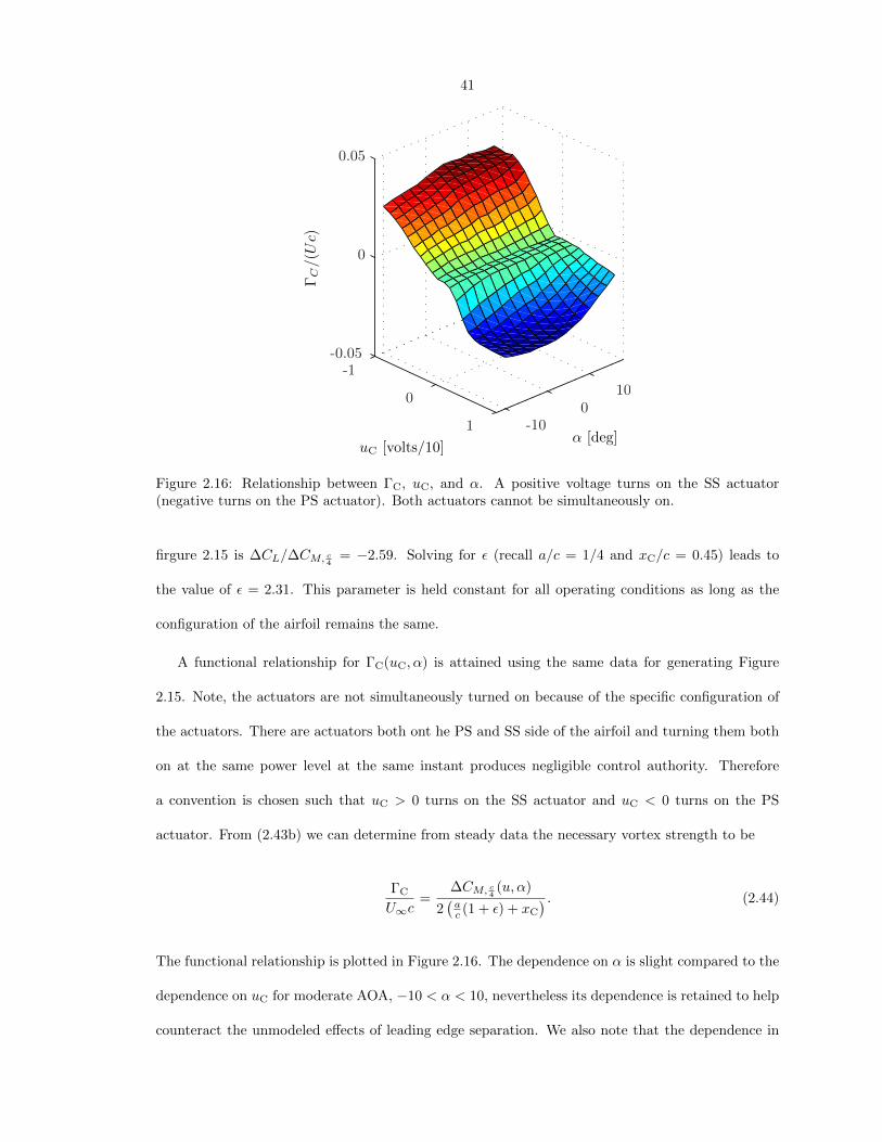
41
uC [volts/10]α [deg]
ΓC
/(U
c)
-1
0
1 -100
10
-0.05
0
0.05
Figure 2.16: Relationship between ΓC, uC, and α. A positive voltage turns on the SS actuator(negative turns on the PS actuator). Both actuators cannot be simultaneously on.
firgure 2.15 is ∆CL/∆CM, c4= −2.59. Solving for ε (recall a/c = 1/4 and xC/c = 0.45) leads to
the value of ε = 2.31. This parameter is held constant for all operating conditions as long as the
configuration of the airfoil remains the same.
A functional relationship for ΓC(uC, α) is attained using the same data for generating Figure
2.15. Note, the actuators are not simultaneously turned on because of the specific configuration of
the actuators. There are actuators both ont he PS and SS side of the airfoil and turning them both
on at the same power level at the same instant produces negligible control authority. Therefore
a convention is chosen such that uC > 0 turns on the SS actuator and uC < 0 turns on the PS
actuator. From (2.43b) we can determine from steady data the necessary vortex strength to be
ΓC
U∞c=
∆CM, c4(u, α)
2(ac (1 + ε) + xC
) . (2.44)
The functional relationship is plotted in Figure 2.16. The dependence on α is slight compared to the
dependence on uC for moderate AOA, −10 < α < 10, nevertheless its dependence is retained to help
counteract the unmodeled effects of leading edge separation. We also note that the dependence in

42
PSfrag replacemen
time [s]
uC
[volts/
10]
0 2 4 6 8 10-1
-0.5
0
0.5
1
(a)
time [s]
α[d
eg]
0 2 4 6 8 10-5
0
5
10
15
(b)
Figure 2.17: Comparison of test bed simulation with experimental results. (a) Input command signalgiven to both the simulation and the experiment (Tchieu et al., 2008). (b) Airfoil response due tocontrol input: current model; experiments.
uC. From this data, a lookup table is used to acquire ΓC for simulation of the equations of motion.
2.5.4 Comparison between experiments
The model equations with the control vortex effects are compared to the experimental setup. For
this case, the airfoil is controlled by the torque motor to hold a specific AOA but with a loosely tuned
controller such that a sufficient control input produces an obvious response in the AOA of the airfoil.
A simulation of the model is created in Matlab Simulink to include the airfoil dynamics described
by the model presented in Section 2.2 with the additional actuator model described in Section 2.5.2 in
addition to the dynamics of the experimental setup depicted in Figure 2.4 undergoing pure pitching
airfoil motion. A Simulink schematic and details of the numerical model for the dynamics of the
experimental setup can be found in appendix A.
43
The controller is first set to hold the airfoil at α = 3. Several doublet commands are given to the
synthetic jet actuators, each of different duration as seen in Figure 2.17(a), and since the controller
is non-aggressive, the airfoil moves substantially. The experimental response (red) and the model
response (blue) are given in Figure 2.17(b). The model equations do a very good job of simulating
the experimental response. A major difference between the simulation and the experiments is that
the airfoil tends to relax to its original position at a much faster rate. This can be attributed to the
unmodeled and excessive damping in the experimental apparatus (Muse et al., 2009).
2.5.5 Simple feedback for reduction of vortex induced oscillations
It has been shown in Section 2.4 that under specific conditions an airfoil will undergo non-stalled
vortex-induced vibrations in the attached flow regime for a sudden change in AOA which may
eventually lead to separation and the onset of stall. In this section, the reduction of such vibrations
is investigated using the actuators modeled above. Assuming that α of the airfoil can be exactly
measured, a simple control law is proposed such that
uC = −KCα. (2.45)
The control can be saturated thus |uC | < 1 at any time. The control strategy is applied to case (f)
in table 2.1 in an attempt to stabilize the system. Seen in Figure 2.18 is the response of the system
when the gain is set to KC = 1. The control gain is lightly tuned in this case and with feedback,
the airfoil is capable of maintaining its stability.
A more sophisticated control strategy is more difficult to design for this case, as the model is
still very highly non-linear due many factors, namely the creation of new vortices. Though not the
primary interest of this author a further application using adaptive control with a linearized version
of the current model applied to the GTRI experiments is found in appendix B.

44
y∗ b
α[d
eg]
uC
t∗0 50 100 150
-1
0
1
-5
0
5
-0.05
0
0.05
Figure 2.18: Simple feedback is used to reduce the induced vibrations on a airfoil in case (f) infigure 2.1.
2.6 Conclusions
A one-equation aerodynamic model has been created to address the issues related with the fluid-
structure interaction of an idealized flat-plate airfoil subject to a free-stream flow. The major
assumptions that are in play here are that the airfoil is at very high Reynolds number and that the
airfoil does not experience any leading edge separation at any instant thus providing a simplified
model for the wake dynamics. The wake dynamics and airfoil circulation distributions are then used
to generate expressions for lift and moment. The resulting equations for lift and moment are then
adjusted accordingly for application to airfoils with thickness and camber.
The model is compared to experiments performed at GTRI and high-fidelity simulations at
University of Texas, Austin of a NACA 4415 wing section at high Reynolds number. The results
are quite promising given the number of assumptions used to simplify the model. For low reduced
frequencies in pitch and plunge, the model gives a good prediction of the aerodynamic lift and
moment. For high reduced frequencies, the agreement is still quite acceptable although the small
scale vortex shedding could not be captured from the simplicity of the model.
Given here are just a few of the problems that can be confronted with this model. The flutter

45
problem is addressed using the model to show, as an example, the use and implementation of the
model for fluid-structure interaction. Several examples of stable and unstable flutter phenomena are
given. Additionally, a multi-modal response is shown for very stiff structures that may break single
bending-torsion mode assumption used for classical flutter analyses.
We note that the model presented here is based on the assumption that no leading edge sepa-
ration occurs. When large-scale leading edge separation occurs, the model does a marginal job of
representing the dominant features in the fluid mechanics and thus does not accurately capture the
lift and moment on the airfoil. This may occur when the airfoil performs maneuvers at high angle-
of-attack or at very fast pitching and plunge rates. In addition, the model becomes less applicable
when the thickness and camber of the airfoil exceed the thin airfoil limit becuase the body may have
separation bubbles on the pressure and suction side. This causes a large departure from the thin
airfoil theory that is formulated here because these separation bubbles are unsteady in nature.
The aerodynamic model is further extended using the concept of trapped vorticity to model
the synthetic jet actuators used in this specific application of airfoil control without conventional
control surfaces. The augmented model is then implemented in a simulation of the experimental
apparatus at GTRI and its comparison to experimental results give very good agreement. With
this validated model, a simple feedback algorithm is used to suppress the vortex-induced vibrations
of a thin airfoil. Even when the airfoil undergoes unsteady flutter, the lightly tuned algorithm can
stabilize the system. Further application of the model in the context of adaptive control can be
found in appendix B.
We note that a more advanced model for the sythetic jets may be formulated for future imple-
mentation to help aid with the discrepancies between the model and the experimental results. For
a more accurate response, the time dependence of the control vortex must be explicitly treated. In
addition, the control vortex may be much more than a function of the control voltage such that it
depends on the state of the fluid dynamics and the shape (e.g. camber) of the airfoil. At this point,
the only reasonable method, without resorting to modeling each pulse period of the synthetic jet
or accounting for specific configurations of the airfoil, is to determine this dependency is through

46
empirical relations.

47
Chapter 3
An inviscid low-order model forthe vortex-induced vibration ofbluff bodies
3.1 Introduction
The ubiquitous nature of vortices in many natural flows have led to various studies of the vortex
dynamics in the past with many using low-order models to provide physical understanding of the
fluid dynamics in free space and near rigid, stationary boundaries. For high Reynolds number two-
dimensional flows, one can expect vortices to behave as compact structures that lose their definition
only over large non-dimensional times due to the slight viscosity. Therefore potential point vortices
make an excellent simplification to the fluid dynamics problem by reducing the complexity of the
governing equations by several orders of magnitude in comparison to direct numerical simulation
techniques of the viscous Navier-Stokes equations. Several studies have investigated stationary bluff
body flows using point vortices with varied success including studies of vortex shedding behind a
square-like section (Clements, 1973), the investigation a flat plate at high angle of attack (Sarpkaya,
1975), and the modeling of separation behind a circular cylinder (Sarpkaya and Schoaff, 1979).
In these instances, the evolution vortex sheet-like structure is essentially simulated by introducing
individual point vortices at each time step at geometrically convenient and or empirically calculated
separation points.

48
Cortelezzi et al. (1994) and Cortelezzi (1996) further simplified these models by introducing
varying strength vortices that followed the so-called Brown-Michael correction (Brown and Michael,
1954, Rott, 1956, Cheng, 1954, Bryson, 1959). Instead of shedding vortices at every time step, a set
of ordinary differential equations is derived for the entire system leading to a system with analytical
solutions for starting flow and a system that can be numerically integrated using standard methods
when more vortices are present. This further reduced the complexity and ad-hoc corrections that
were introduced in previous methods.
Until recently the treatment of coupled fluid-structure intereaction (FSI) between point vortices
and a single rigid body have not been rigorously treated. Jones et al. (2005) and Shukla and Eldredge
(2007) use a vortex sheet representation with the corresponding Birkhoff-Rott integro-differential
equation and derived a model to determine the FSI between falling cards and the deformation of a
heaving flexible plate, respectively. Moreover, the equations of a body interacting with one or more
pre-existing point vortices in an ideal, two-dimensional fluid are derived in Borisov et al. (2007a) as
an extension of Ramodanov (2002) and Borisov et al. (2005) following a dynamical systems approach,
in addition to the concurrent work performed by Shashikanth (2005). Roenby and Aref (2010) used
a similar approach and investigated the integrability of such equations in the context of transition to
chaotic motion. Furthermore, Michelin and Smith (2009b) studied the FSI generated by a general
sharp-edged body with the Brown-Michael correction in order to study the broadside fall of a thin
plate among other studies of FSI (Michelin et al., 2008, Michelin and Smith, 2009a).
In this chapter, we develop a general method to treat the FSI of a bluff body in the presence
of a freestream flow and/or multiple vortices. It is chosen to also concentrate on the canonical
two degree-of-freedom spring-damper system model of vortex-induced vibration since it is one of
the simplest FSI to consider and has various implications in the study of FSI. Previous models of
vortex-induced vibration relied heavily on empirical data (Gabbai and Benaroya, 2005, Benaroya
and Gabbai, 2008). In many cases, such as wake-oscillator models, the fluid dynamics are nearly
non-existent in the description of the model itself. The present model will provide better insight
into the interactions of vortices with the canonical mass-spring-damper system for vortex-induced

49
iy
x
!2, z2
!1, z1
!3, z3 z1,s
z2,s
. . .!n, zn
!
z0
U!
z-plane
(physical plane)
zb
Tuesday, August 10, 2010
(a)
!
i!
. . .
!n, !n
!1, !1!2, !2
!3, !3
!2,s !1,s
!-plane
(mapped plane)
Tuesday, August 10, 2010
(b)
Figure 3.1: Schematic of a body interacting with N point vortices in the physical-plane and themapped-plane. As an example, two variable strength vortices are illustrated with an attacheddotted line to indicate vortex shedding and growth of the vortex. (a) z-plane. (b) ζ-plane.
vibration.
Two specific geometries are more closely investigated. First we consider the case where a circular
cylinder interacts with pre-existing vortices in the flow with and without a freestream flow. The
introduction of vortices is not addressed in this situation because the inviscid shedding off smooth
bodies is an ongoing research topic that is difficult to model. In the case where the freestream is
present, we specifically investigate how the vortices excite the modes of oscillation and what kind of
responses can be expected.
In the second case, the FSI of a flat plate with vortices is given as an example. The application
of a new vortex shedding model is used for this flow. As a test, we first apply the shedding model
to a stationary plate and see the resultant vortex motion and shedding cycle to gain confidence in
the fluid dynamics. Following this, we apply the model to a vortex-induced vibration case to see a
sample response of the system due to the modeled vortex shedding.

50
3.2 General formulation
Consider the problem as depicted in Figure 3.1(a) in the z-plane where N point vortices of strength
Γn and location zn interact with a rigid two-dimesnional solid with centroid location z0 and orienta-
tion defined by θ. Of the N vortices, P vortices are considered to have varying strengths to represent
circulation shed from the body (in Figure 3.1(a) these vortices are shown with the attached dotted
lines). The body is allowed to translate at velocity z0 and rotate at an angular rate Ω = θ based
on the interactions with the vortices and the freestream flow. We seek an incompressible, inviscid
potential flow solution for the fluid in an unbounded domain such that the boundary conditions on
the body’s surface, ∂D0, are satisfied. To accomplish this, conformal mapping is used to transfer the
problem at hand from the physical plane to a more manageable configuration in the mapped-plane
(ζ-plane) as depicted in Figure 3.1(b).
3.2.1 Conformal map
The conformal map that takes the circle, |ζ| = a, in the mapped-plane to the the physical boundary
in the z-plane with centroid located at z0 and orientation θ can be written as
z = z0 + eiθg(ζ). (3.1)
For now, we restrict g(ζ) ∼ ζ as z → ∞. More specific examples of the function will be given in
sections 3.3 and 3.4.
3.2.2 Boundary conditions and associated potentials
The solution for the complex potential is a linear combination of the individual contributions due
to the flow generated by the translation of the body, Wt, the rotation of the body, Wr, the free
stream, Wf, and each vortex, Wn,v. For the translational potential, the required boundary condition
is such that the normal velocity is exactly balanced by the normal velocity of the body. In complex

51
notation, this reduces to
Re
[−idW
ds
]= Re
[−iz0
dz
ds
](3.2)
where s is taken along the body. After integrating (3.2) with respect to s and noting that Re [−iWt] =
Im [Wt] it is found that the streamfunction satisfies
Im [Wt] = Im[z0z], on ∂D0. (3.3)
This is another manifestation of the common Schwarz problem and when transfered to the mapped-
plane on |ζ| = a, it can be solved by using the Poisson integral formula (or with subtle geometric
formulas). The solution to (3.3) given in terms of ζ is
Wt = U (ζ − g(ζ)) +a2U
ζ(3.4)
where U = −z0eiθ.
Similarly for the rotational potential, it is required that
Re
[−idWr
ds
]= Re
[iΩ (z − z0)
dz
ds
]
and upon integration, the potential satisfies
Im [Wr] = Im
[−iΩ
(1
2zz − zzk
)], on ∂D0. (3.5)
The solution for Wr in terms of ζ is not obvious and must be found on a case to case basis depending
on the mapping function g(ζ) in (3.1). For now, the solution satisfying (3.5) is denoted
Wr = wr(ζ). (3.6)
Several examples of such potentials can be found in appendix C.

52
For the freestream and vortex potentials, it is required that the streamfunction satisfies the no
flow-through condition
Im [Wf] = Im [Wn,v] = constant, on ∂D0. (3.7)
The solution for the freestream potential can be found using geometric relationships and is
Wf = U∞
(ζeiθ +
a2e−iθ
ζ
). (3.8)
The potential for a single vortex can be found using the circle theorem (Milne-Thomson, 1968) and
is simply
Wn,v =Γn2πi
log
ζ − ζnζ − a2
ζn
. (3.9)
Adding Equations (3.4), (3.6), (3.8), and N instances of (3.9) gives the solution to the potential
problem
W = U (ζ − g(ζ)) +a2U
ζ+ wr(ζ) + U∞
(ζeiθ +
a2e−iθ
ζ
)+
N∑
n=1
Γn2πi
log
ζ − ζnζ − a2
ζn
. (3.10)
Note that there are an infinite number of solutions to the boundary value problem. A vortex can
always be added at ζ = 0 and still satisfy the zero normal velocity boundary condition. This is
commonly referred to as the “bound vortex.” It is our interest to study cases where the circulation
is zero for all time in the entire domain, therefore this bound vortex is removed.
3.2.3 Definition of the velocity
The velocities in the physical plane are defined as
u− iv =dW
dz(3.11)
=dW
dζ
/dz
dζ(3.12)

53
recalling the relation that W = W (z) = w(ζ(z)). The definitions given in (3.4), (3.8), and (3.9) are
differentiated and substituted into (3.12) to give
dW
dz=
e−iθ
g′(ζ)
(U∞
(ζ2eiθ − a2e−iθ
ζ2
)+ U (1− g′(ζ))− a2U
ζ2
+ w′r(ζ) +
N∑
n=1
Γn2πi
(1
ζ − ζn− ζnζζn − a2
))(3.13)
where the prime denotes differentiation with respect to ζ.
3.2.4 Equation of motion for vortices
We use a more generalized form of the standard Kirchoff laws of vortex motion. Unlike previous
studies involving point vortex models this equation accounts change in motion due to the growth of a
vortex provided that the location at which circulation is being fed is given (Cortelezzi and Leonard,
1993). This provides a means for circulation to be shed into the wake and it degenerates into the
standard Kirchoff law when the vortex remains at constant strength.
Vortices convect with the Brown-Michael law, which mandates that a growing vortex and its
associated branch cut must convect force free. With this constraint, the equation of motion for nth
vortex in the physical plane, whether being fed or not, is governed by
zn + (zn − zn,s)ΓnΓn
=
(dWn
dz
)(3.14)
where zn,s is the generating corner for the vortex (see Figure 3.1(a)) and the (˙) represents the time
derivative, ddt . The function on the right hand side of (3.14) is defined as the desingularized velocity
field such that
dWn
dz=
e−iθ
g′(ζn)
(dWn
dζ− Γn
4πi
(g′′(ζn)
g′(ζn)
))(3.15)

54
where
Wn = W − Γn2πi
log (ζ − ζn) (3.16)
is the desingularized complex potential. The extra term on the right hand side of (3.15) is the so-
called Routh correction and it stems from rewriting (3.14) in terms of mapped-coordinates (Clements,
1973). In the case where a vortex has reached a constant strength, i.e., is no longer being fed
circulation, then the vortex velocity follows the standard Kirchoff evolution equation
zn =
(dWn
dz
). (3.17)
The equations of motion are most comfortably solved in the ζ-plane, therefore (3.14) is rewritten
as
eiθg′(ζn)ζn + z0 + iΩeiθg(ζn) + eiθ (g(ζn)− g(ζn,s))ΓnΓn
=
eiθ
g′(ζn)
[U∞
(ζ
2
ne−iθ − a2eiθ
ζ2
n
)+ U
(1− g′(ζn)
)− a2U
ζ2
n
+ w′r(ζn)
−N∑
j 6=n
Γj2πi
(1
ζn − ζj− ζj
ζnζj − a2
)+
Γn2πi
(ζn
ζnζn − a2+g′′(ζn)
2g′(ζn)
)]. (3.18)
3.2.5 Force
An expression for the force, F , is given in Sedov (1965) as
Fρf
= i
N∑
n=1
zn,sΓn +i
2
∮
∂D0
(dW
dz
)2
dz + id
dt
∮
∂D0
zdW
dzdz +Az0 (3.19)
where A denotes the area of the solid body. Equation (3.19) is a variation of the more standard
unsteady Blasius integral equation for force that is most commonly used in various references (Milne-
Thomson, 1968, Graham, 1980, Cortelezzi, 1996). In essence, all forms of the force integrals are
derived by integrating the pressure force on the surface, but there are several key simplifications

55
!D!
!D1
!D2
!Dn!D0
Saturday, August 14, 2010
Figure 3.2: Schematic of the application of Cauchy’s theorem to deform ∂D0 to form the contours∂D∞, ∂Dn, and the associated contours connecting the two. The infinitessimally thin contoursconnecting ∂Dn to ∂D∞ contribute nothing to the integrals in (3.19) because the integrands areanalytic in the fluid domain.
made to obtain (3.19) so that the integration is more manageable. In particular, the time derivative
given in the third term on the right hand side of (3.19) is taken out of the integrand whereas in the
standard unsteady Blasius equation, it remains within.
We can further simplify the expression given in (3.19) by following Michelin and Smith (2009b)
and applying Cauchy’s theorem. This allows us to extend the contour ∂D0 to the contour given in
Figure 3.2 which consists of a contour at infinity, ∂D∞, and several infinitesimally small contours
around each vortex, ∂Dn, in the opposite sense. Therefore the integrals in (3.19) can be written as
∮∂D0
=∮∂D∞
−∑Nn=1
∮∂Dn
. To make further progress, we expand the potential at z →∞ to read
W = a1z + a0 +a−1
z+a−2
z2+O
(1
z3
), as z →∞ (3.20)
and subsequently after term by term differentiation
dW
dz= a1 −
a−1
z2− 2a−2
z3+O
(1
z4
), as z →∞ (3.21)
where the coefficients aj are time dependent. In addition, near each vortex, the complex velocity

56
can be expanded as
dW
dz=
Γn2πi
(1
z − zn
)+
dWn
dz+O(z − zn), as z → zn. (3.22)
Upon substitution of (3.20), (3.21), and (3.22) into (3.19), the force reduces to
Fρf
= −i[N∑
n=1
(Γnzn + Γn (zn − zn,s)− Γnwn
)+ 2πia−1
]+Az0. (3.23)
If the Brown-Michael model (3.14) for growing vortices is used then (3.23) simplifies to
Fρf
= 2πa−1 +Az0. (3.24)
The details of the determination of a−1 is addressed in specific examples given in sections 3.3 and
3.4 because it depends on the choice of the mapping function, g(ζ).
3.2.6 Torque
Sedov (1965) also provided an equation for torque, T , which is extended in Michelin and Smith
(2009b) to the case where the center of mass of the body moves with location z0(t). This latter
expression is given as
Tρf
=1
2
N∑
n=1
|zn,s − z0|2Γn +1
2Re
[2z0
∮
∂D0
(z − z0)dW
dzdz
−∮
∂D0
(z − z0)
(dW
dz
)2
dz +d
dt
∮
∂D0
|z − z0|2dW
dzdz
]. (3.25)
The same technique that is applied in Section 3.2.5 can be used to deform the contour ∂D0 to
simplify (3.25) to read
Tρf
=1
2
N∑
n=1
|zn,s − z0|2Γn + Re
[N∑
n=1
(dWn
dz− z0
)(zn − z0) Γn − 2πiz0a−1 + 2πia1a−1
]+B2
(3.26)

57
where
B = Re
[∮
∂D0
|z − z0|2dW
dzdz
]. (3.27)
Although it seems (3.27) is not analytic, given the mapping g(ζ), it can be integrated by noting that
z(ζ) remains analytic on the boundary. Since the function is analytic on the boundary, it can be
analytically continued into the domain and integrated using standard complex methods.
3.2.7 Coupled equations of motion
Assuming that there is an external force Fe and torque Te, the coupled equations of motion for the
bodies are simply
(m− ρfA)z0 = 2πρf a−1 + Fe (3.28)
and
Iθ =ρf
2
N∑
n=1
|zn,s − z0|2Γn + ρf Re
[N∑
n=1
(dWn
dz− z0
)(zn − z0) Γn
− 2πiz0a−1 + 2πia1a−1
]+ρfB2
+ Te (3.29)
where m and I are the mass and mass moment of inertia of the body about the centroid, respectively.
The Equations (3.18), (3.28), and (3.29) constitute 2N + 3 equations. If the strength of all vortices
are held fixed (Γn = 0) then we have 2N + 3 unknowns (2N vortex positions, two body positions,
and one angular orientation) and the problem can be integrated given sufficient initial conditions.
3.3 Vortex-induced vibrations of a circular cylinder
Here we model the induced vibrations of a circular cylinder and a spring-damper system that is
depicted in Figure 3.3 with an additional N constant strength vortices. We are not concerned with

58
U!
z0
kz, bz
kz, bz
N!
n
!n, zn
Tuesday, August 24, 2010
Figure 3.3: Schematic of the vortex-induced vibration for a circular cylinder in cross flow. Thereare two degrees of freedom for the solid structure, x and y.
vortex growth since it is difficult to model separation off smooth bodies using inviscid methods
(Sarpkaya and Schoaff, 1979). The presence of the spring-damper system is modeled by setting the
external force to
Fe = −kz(z0 − zE)− bz z0 (3.30)
where kz and bz are both scalars and represent the stiffness and damping constant, respectively.
The location zE represents the equilibrium position such that the cylinder feels no force from the
stiffness.
3.3.1 Equations of motion
In this specific case, due to the geometry of the problem, the orientation θ is not used and thus
removed from the equations of motion. In addition, it is not necessary to calculate torques about
the centroid (it will be zero by definition). Although we can treat the system without a specific
map, one is chosen to stay within the framework presented in Section 3.2, therefore the conformal
map for this case is
z = z0 + ζ (3.31)

59
which just offsets the cylinder at a location z0. Given the map, the potential can be determined by
(3.10) and is
W =a2z0
ζ+ U∞
(ζ +
a2
ζ
)+
N∑
n=1
Γn2πi
log
(ζ − ζnζ − a2
ζn
). (3.32)
Performing a series expansion at z →∞ gives
a−1 = a2(z0 + U∞) +
N∑
n=1
Γn2πi
(a2
ζn− ζn
). (3.33)
The equation of motion for the body is found by substituting (3.30) and (3.33) into the equation of
motion for the body, (3.28), and explicitly expanding the time derivative to give
(ρb + ρf)πa2z0 + bz z0 + kz(z0 − zE) = iρf
N∑
n=1
Γn
(ζn +
(a2
ζ2
n
)ζn
)(3.34)
where ρb is the uniform density of the body. Note that the Γn = 0 for all n since the vortex strengths
are restricted to be constant and pre-existing.
Upon substitution of (3.32) into Equation (3.18), the motion of the vortices for this specific case
is governed by
ζn = −z0 +
(a2
ζn
)z0 + U∞
(1 +
a2
ζn
)−
N∑
j 6=n
Γj2πi
(1
ζn − ζj− ζj
ζjζn − a2
)+
Γn2πi
(ζn
ζnζn − a2
)
(3.35)
The combination of (3.34) and (3.35) together gives 2N + 2 equations for the 2N + 2 unknowns (2N
vortex positions, ζn, and two from the position, z0) therefore we can solve the system readily using
a standard numerical integrator.

60
3.3.2 Results
Elastically mounted cylinder
Klamo (2007) presented various cases for which a single degree-of-freedom cylinder undergoes large
amplitude vortex-induced vibration under the presence of a freestream velocity. Although, in ac-
tuality, the induced vibration is created by the unsteady bluff-body shedding, here we choose to
examine a specific case of the vortex-induced vibration of in the presence of pre-existing vortices.
In the stationary flow case, this may be thought of as ocean eddies interacting with off-shore risers.
The spring stiffness and damping are prescribed as kz = 1 and bz = 0 such that the structural
natural frequency in vacuum is ωs =√
1/π (ρf = 1, a = 1). In addition we enforce that the fluid
is neutrally buoyant such that the density of the cylinder is simply ρb = ρf. These are found to be
typical values for which we can expect a large amplitude response in the canonical one-degree of
freedom case (Klamo, 2007).
The response of an elastically mounted cylinder is studied in the presence of pre-existing vortices.
There is no freestream flow in the cases considered (U∞ = 0) . First, the effect of a single vortex on
the structure is explored. Γ1 is selected so that Γ1/(ωsD
2)
= 1. The simulation is initialized with
a vortex located at z1(t = 0) = x1 > D/2 and the structure is allowed to interact with it. Plotted
in Figure 3.4 is a typical response for this case. As seen in Figure 3.4(a) the motion of the vortex
and the cylinder does not follow any particular periodic structure. It is seen in Figure 3.4(b) that
the amplitudes oscillations are substantial.
We can attempt to find a maximum amplitude of oscillation, A∗ = max (|z0|) /D, given a starting
vortex location, z1(t = 0). The simulations are run until tωs = 1000 at which point the maximum
displacement over all time is used to determine the maximum non-dimensional amplitude. This is
plotted in Figure 3.5. We can see that there is not a simple relationship. Unexpectedly, when the
vortex is very close to the cylinder, its effect is very small. The vortex tends to encircle the cylinder
at a very quick rate while avoiding changing its inertia. As the distance is increased, the cylinder
begins to oscillate until it reaches a maximum amplitude over time with an initial vortex location

61
x/D
y/D
-1 0 1
-1
-0.5
0
0.5
1
(a)
ωst
|z 0|
0 50 100 150 200 2500
0.1
0.2
0.3
0.4
0.5
(b)
Figure 3.4: Response of the system for z1(t = 0)/D = 0.930 with kz = 1 and bz = 0 at t = 500. (a)Cylinder path (black) and vortex path (blue), represents the initial locations of the vortices. (b)Time history of the amplitude of the cylinder response, |z0|.

62
z1/D
A∗
0.5 1 1.5 20
0.1
0.2
0.3
0.4
0.5
0.6
Figure 3.5: Maximum amplitude versus vortex separation distance, z1/D. kz = 1, bz = 0 Γ1 =ωsD
2 = 2.2568.
at z1(t = 0)/D = 0.93.
As more vortices are added, the system appears to become chaotic. This is partly due to the fact
that when there is more than one vortex interacting with a circular cylinder, chaotic motion ensues
because of the system is no longer integrable (Roenby and Aref, 2010). We can see this behavior
in an example given in Figure 3.6. For a relatively short time, the motion of the cylinder seems
erratic. With a slight change in initial conditions, the response becomes drastically different. An
effort has been made to find the maximum amplitudes for this case and although the response is
always bounded, there was no trend due to the chaotic nature of the flow.
Elastically mounted cylinder with cross-flow
Here vortices are released upstream of the circular cylinder and allowed to convect downstream and
interact with the circular cylinder. The system is initialized with a vortex street ahead of the cylinder
as depicted in Figure 3.7. The parameters δx and δy define the spacing for the incoming street.
The first vortex of the street is located 10 convective time units upstream. We choose δy/D = 0.5
so that the street impinges on the cylinder initially with the width equal to the cylinder diameter.
A Strouhal number is defined such that St = fvD/U where fv is the frequency of the oncoming
vortices. In this case, fv = U/(δx) therefore St = D/(δx). We restrict our attention to the case

63
x/D
y/D
-1 0 1
-1
-0.5
0
0.5
1
1.5
(a)
ωst
|z 0|
0 50 100 150 2000
0.2
0.4
0.6
0.8
1
(b)
Figure 3.6: Response of the system for z1(t = 0)/D = 1.275 and z2(t = 0)/D = 1.275i with kz = 1and bz = 0 at t = 100. (a) Cylinder path (black) and vortex path (blue, green), represents theinitial locations of the vortices. (b) Time history of the amplitude of the cylinder response, |z0|.
U!
!y!x
Tuesday, August 24, 2010
Figure 3.7: Schematic defining the parameters in the vortex street.

64
A∗ x
St
0.15 0.2 0.25 0.3 0.350
1
2
3
4
(a)
A∗ y
St
0.15 0.2 0.25 0.3 0.350
1
2
3
4
(b)
Figure 3.8: Max displacement versus Strouhal frequency of incoming vortex street. (a) x-direction.(b) y-direction.
ωst
x0/D
0 50 100 150 200-4
-2
0
2
4
(a)
ωst
y 0/D
0 50 100 150 200-4
-2
0
2
4
(b)
Figure 3.9: Displacement versus time for St = 0.25. (a) x-direction. (b) y-direction.
where kz = 1 and bz = 0.1.
Given in Figure 3.8 are the max amplitudes in the x and y-direction for a given Strouhal number
for the chosen parameters. As the body starts to vibrate at higher transverse amplitudes, the
incoming vortices begin to have a larger influence because they almost hit the structure near head-
on (recall δy/D is set to one half). This causes a larger force on the cylinder and more feedback
until the system saturates as seen in Figure 3.9(b). This type of large amplitude behavior happens
near ωs.

65
k!, b!U!
!z0
kz, bz
kz, bz
N!
n
!n, zn
Tuesday, August 24, 2010
Figure 3.10: Schematic of the vortex-induced vibration for a flat plate in cross flow. There are threedegrees of freedom for the solid structure; x, y, and θ.
3.4 Vortex-induced vibration of a flat plate at high angles of
attack
We model the induced vibrations of a plate and spring-damper system that are depicted in Figure
3.10. For the body itself, there are three degrees of freedom, x0, y0, and θ. In this example, the
vortex strengths are not restricted to be constant. In fact, a separation model is also presented to
allow circulation to enter the fluid from the two sharp edges of the plate.
Again, the spring-damper system in the x and iy directions is modeled by (3.30). In addition,
there is an additional spring-damper system added such that
Te = −kθ(θ − θE)− bθΩ (3.36)
where kθ and bθ represent the stiffness and damping constant in the θ direction, respectively. The
equilibrium angle is chosen to be θE = π2 so that the freestream flow impinges on the plate in a bluff
fashion.

66
3.4.1 Equations of motion
The mapping taking the circle to a flat plate of length, l = 4a is given by
g(ζ) = ζ +a2
ζ. (3.37)
For the mapping (3.37), the potential satisfying the associated boundary conditions in the ζ-plane
is given by
W = U∞
(ζeiθ +
a2
ζe−iθ
)− 2ia2Im [U ]
ζ− iΩa4
ζ2−
N∑
n=1
iΓn2π
log
ζ − ζnζ − a2
ζn
(3.38)
where details of deriving the rotational potential, wr(ζ) = −iΩa4/ζ2, are given in appendix C. Upon
substitution of (3.38) into (3.18) the equation of motion for the nth vortex is
(ζ2n − a2
ζ2n
)ζn +
((ζn − ζn,s)2
ζnΓn
)Γn = U − iΩ
(1 +
a2
ζn
)
+ζ
2
n
ζ2
n − a2
[U∞
(e−iθ − a2
ζ2
n
eiθ
)− 2ia2Im [U ]
ζ2
n
− 2iΩa4
ζ3
n
−N∑
j 6=n
Γj2πi
(1
ζn − ζj− ζj
ζnζj − a2
)+
Γn2πi
(ζn
ζnζn − a2+
a2
ζn(ζ2
n − a2)
)]. (3.39)
To determine the equations of motion for the body, we perform a series expansion on (3.38) to give
a1 = U∞ and
a−1 = eiθ
(−2ia2 (U∞ sin θ + Im [U ]) +
N∑
n=1
Γn2πi
(a2
ζn− ζn
)). (3.40)
Substituting (3.38) and (3.40) into the coupled linear momentum equation, (3.28) becomes
m
ρfe−iθ z0 − 4πia2Im
[z0eiθ
]+bz z0 + kz(z0 − zE)
ρfe−iθ = −4πia2 (ΩU∞ cos θ + Im [iΩU ])
+ Ω
[4πa2 (U∞ sin θ + Im [U ])−
N∑
n=1
Γn
(ζn −
a2
ζn
)]+ i
d
dt
N∑
n=1
Γn
(ζn −
a2
ζn
). (3.41)

67
Additionally, from (3.29) the angular degree of freedom is dictated by
IΩ
ρf− B
2−1
2
2∑
n=1
∣∣∣∣(ζn,s +
a2
ζn,s
)∣∣∣∣2
Γn +bθΩ + kθ(θ − θE)
ρf=
Re
[N∑
n=1
Γn
(dWn
dz− z0
) (ζn +
a2
ζn
)eiθ − 2πia−1
(z0 − U∞
)]
(3.42)
where a−1 is defined in (3.40), the derivative of B is given as
B = −4πa4Ω− 2a2N∑
n=1
(−2Γna
2Re
[ζnζ3n
]+ Γn
(a2Re
[1
ζ2n
]+ 1
)), (3.43)
and the vortex velocity is defined as
dWn
dz=
ζ2ne−iθ
ζ2n − a2
[U∞
(eiθ − a2
ζ2n
e−iθ)
+2ia2Im [U ]
ζ2n
+2iΩa4
ζ3n
+
N∑
j 6=n
Γj2πi
(1
ζn − ζj− ζj
ζnζj − a2
)− Γn
2πi
(ζn
ζnζn − a2+
a2
ζn(ζ2n − a2)
)]. (3.44)
If all vortices in the flow are constant strength (i.e. pre-existing) all terms involving Γn = 0.
This leads to 2N + 3 unknowns (2N vortex locations, ζn, two from z0, and one from the orientation,
θ). The combination (3.39), (3.41), and (3.42) give 2N + 3 real valued equations (two per complex
equation). Again, a standard scheme is used to integrate the system.
3.4.2 Separation model and the Kutta condition
A shedding model can be conveniently derived for the current problem because of the existence of
the two sharp edges on the plate. The complex velocity given by (3.13) is
u− iv =ζ2e−iθ
ζ2 − a2
[U∞
(eiθ − a2
ζ2e−iθ
)+
2ia2Im [U ]
ζ2+
2iΩa4
ζ3+
N∑
n=1
Γn2πi
(1
ζ − ζn− ζnζζn − a2
)].
(3.45)
Upon closer inspection, (3.45) indicates that at the sharp edges ζ = ±a there exists an inherent
singularity due to the mapping function. It is reasonable, but not entirely necessary to remove

68
the singularity at the sharp edges as the system of equations can still be integrated (albeit the
velocities near the sharp edges remains unphysical). However, the removal of the singularity can
conveniently model the effect of inviscid shedding as well. To do so, one can introduce two vortices,
Γ1(t) and Γ2(t), near the tips to remove the singularity. The strength of these vortices is continually
adjusted such that the velocity in the frame of the plate is zero at the tip. This is known as applying
the unsteady Kutta condition (Cortelezzi and Leonard, 1993). Defining the pseudo-velocity as the
interior of the bracketed term in (3.45), dWdζ , the Kutta condition can be written as
dW
dζ
∣∣∣∣ζ=±a
= 0. (3.46)
or, when simplified,
Im[U∞eiθ + U
]± Ωa±
∑ Γn4πa
(2Re
[ζn
ζn ∓ a
]− 1
)= 0. (3.47)
This condition gives two additional algebraic constraints to the equations of motion by effectively
adjusting the strength of the shedding vortices, Γ1 and Γ2. This naturally allows a method to
introduce circulation into the fluid domain and can be thought of as a model of the separation of a
shear layer feeding the two growing vortices.
Vortex shedding criteria
Subsequent vortices can be shed as well. When a vortex grows, one can expect it to become a free
vortex at some point and allow an incipient vortex to take its place near the generating tip. The
inception of a new vortex can be chosen such that when the rate of change of the strength of the
nascent vortex changes sign (e.g. Γ1 = 0), a new vortex is formed at the sharp tip, as proposed in
Section 2.2.4. There is a problem with this specific shedding model for the current geometry that is
also inherent in other bluff body flows using an inviscid point vortex model. Consider the plate at a
large angle of attack as depicted in Figure 3.10. It is expected that at ζ = a, the corner only feeds
negative circulation to the nascent vortex. If the model previously proposed is used in this instance,

69
PSfrag replacemen
z1,s
z2,s
!1, z1
!2, z2
!1, z1
!2, z2
!1, z1
z2,s
z1,s z1,s
z2,s
Sunday, August 15, 2010
(a)
PSfrag replacemen
z1,s
z2,s
!1, z1
!2, z2
!1, z1
!2, z2
!1, z1
z2,s
z1,s z1,s
z2,s
Sunday, August 15, 2010
(b)
PSfrag replacemen
z1,s
z2,s
!1, z1
!2, z2
!1, z1
!2, z2
!1, z1
z2,s
z1,s z1,s
z2,s
Sunday, August 15, 2010
(c)
Figure 3.11: Schematic showing the instantaneous stagnation streamline at various instants of time.(a) At the inception of both vortices after impulsive start. (b) At an instant prior to pinch off of Γ2.(c) The inception of a new vortex where the new vortex is reindexed to Γ2.
the vortex continues to grow and never pinches off since Γ1 is always negative. This is contrary to
the observation that a von Karman vortex street is nearly always seen in the wake of a bluff body.
Although the increasing complexity of using vortex sheets as opposed to point vortices can
overcome this problem (Jones, 2003), the following scheme is chosen to combat the issue. Shortly
after two vortices are initiated, if the plate is not exactly perpendicular to the flow, the leading
edge vortex usually recirculates flow such that there is a relative stagnation point on the backside
of the plate (i.e., where the velocity relative to the body is zero). This situation is depicted in
Figure 3.11(a). At a later time (Figure 3.11(b)) the relative stagnation point moves towards Γ2.
It is proposed that in addition to the previously described shedding criteria, when the stagnation
point reaches the opposite sharp tip (in this case z2,s), the vortex being fed from that point (Γ2) is
released and an incipient vortex is introduced at the at the tip. A time shortly after this criteria
is illustrated in Figure 3.11(c). Numerically, this is executed by tracking the velocity at a position
zp,0 on the backside of plate near zp,s (p = 1, 2) and determining whether there is a switch in the
the sign of the tangential velocity. The direction of the switch indicates the direction in which the
stagnation point passes through zp,0. At this point, if the direction is consistent with moving away
from the generating edge, then a new vortex is created and the vortices are re-indexed such that the
newly created vortex becomes indexed p = 1 or 2.

70
Incipient behavior of vortices
The flow around the sharp corners can lead to the introduction of a vortex near the edge. As
indicated in Cortelezzi and Leonard (1993) and more recently in Michelin and Smith (2009b), the
introduction of a vortex at the sharp edges creates a singularity since the vortex and its image lie at
the same location and the equation of motion for the nascent vortex cannot be readily integrated.
Thus, due to the singularity, the initiation of the nascent vortex must be treated separately. A
small-time expansion can be used to further unveil the behavior of newly formed vortices from these
edges. Here we summarize the main results of the small time expansions presented in Michelin and
Smith (2009b) and give a procedure for dealing with the situation where the flow is impulsively
started and the case where a vortex is created at the tip with pre-existing vortices in the flow.
In what follows we only consider the vortex that initiates at ζ1,s = a. The vortex that initiates
from ζ2,s = −a can be treated in a similar manner to give essentially the same result. At time
t = 0+ the freestream is impulsively started with the plate at high angle of attack. We define
ζ1 = a(1 + ζ1) such that |ζ1| 1. Closely following Michelin and Smith (2009b), a small time
expansion is performed on the equations of motion and it is found that the leading order behavior
for the vortex position follows
ζ1 = C1eiπ4 t
13 (3.48)
where C1 is a constant. Since z1−a = aeiθ ζ21 , the dominant flow around the corner forces the vortex
to move perpendicularly away from the plate at a power law of t23 without regard for the orientation
of the plate. Consequently, when the Kutta condition is applied, the strength of the vortex grows
like Γ1 ∼ −t13 .
For subsequent vortices, the situation is more difficult to handle. When a vortex is shed from
ζ = a at t = ts, a new vortex is started in its place and the remaining vortices are re-indexed so
the nascent vortex replaces the shed vortex. This new vortex is qualitatively different from the
starting flow vortex because the background flow is essentially canceled due to the satisfaction of
the Kutta condition. It is seen in Michelin and Smith (2009b) that the small-time expansion in this

71
instance leads to the vortex shedding with linear growth in the direction tangent to the sharp edge,
i.e. z1 − a = C2eiθ(t − ts) where C2 is a constant. This imposes two situations. Depending on the
sign of C2 the vortex can either shed away from the tip into the flow or along the plate. The prior
situation is amenable and the latter is very problematic because the inviscid model cannot handle
this situation because the vortex and its image will be one and the same. The problematic case
often occurs at low angles of attack and can also arise when free vortices move in close proximity
to either sharp corner. This is a major drawback of this method. This difficulty is also observed in
inviscid vortex sheet models such as Jones (2003) as well. To the author’s knowledge, this condition
cannot be easily circumvented if encountered. Therefore, we halt the simulation when this condition
occurs. The proximity of free vortices to the sharp edges is not an issue in this case because they
will be sufficiently swept away downstream by the oncoming flow in the cases we consider.
As for the details of numerical implementation, for the impulsive start, a vortex is initiated
perpendicular to each tip at a small distance δ ∼ O(∆t23 ) where ∆t ∼ O(10−5). To determine
the Γp, the Kutta condition is applied. Subsequently, a standard time integrator is used until the
criteria to shed a new vortex is met at t = ts. At this time a new vortex is started, but this time
it is initiated at t = ts + ∆t tangentially at a distance δ ∼ O(t− ts). The integration resumes until
the criteria for shedding is met again, then a new vortex is shed, and so on.
3.4.3 Results
Stationary plate with cross-flow and shed vortices
The vortex shedding criteria is first verified to provide reasonable results. We incline a plate at 45
angle of attack with an impulsively-started oncoming freestream. The radius of the circle in the
ζ-plane is chosen to be a = 1/2, thus the chord length is c = 2. The streamlines for various instants
in time are plotted in Figure 3.12. Figure 3.12(a) demonstrates the starting flow around the plate
forming two vortices, one of which stays attached to the leading edge for some time and another that
moves downstream after initially forming. The stagnation point resulting primarily from the leading
edge vortex moves down the plate in Figure 3.12(b) and eventually pinches off the trailing edge

72
(a) t = 0.4 (b) t = 4.6
(c) t = 8.0 (d) t = 16.0
Figure 3.12: Streamlines at various instants in time for separated flow off of a plate at angle ofattack of 45.
vortex causing a new vortex to be formed in Figure 3.12(c). One key difference seen in comparison
to the results of some more detailed computations is that in the present method subsequent shed
vortices have a much more substantial upwash (Sarpkaya, 1975, Kiya and Arie, 1977). This may be
due to an excess amount of circulation that each vortex gathers before meeting the criteria of being
shed into the wake. Although a slightly high for a bluff body flow, the long time separation Strouhal
number is still reasonable at St ≈ 0.20.
Example of plate vibration due to shed vortices
In this example the plate is only allowed to rotate about its center of mass, that is, z0 is held fixed.
The simulation is initialized with θ0 = π/2. Two vortices are artifically placed far downstream of
the plate to break the flow symmetry thus inducing the von Karman instability in the wake. Other
parameters chosen for this simulation are I = 1, kθ = 1, and bθ = 0. The instability then induces
a rotational oscillation in the system shown in Figure 3.13. The simulation is run until the model
is no longer valid, i.e. when the velocity at the tip of the plate overcomes the oncoming flow such
that a positive (negative) vortex is shed from the top (bottom) separation point. The oscillation of

73
tU/D
θ−
π/2
[rad]
0 10 20 30 40-1
-0.5
0
0.5
1
Figure 3.13: Evolution of θ in vortex-induced vibration of a plate.
the plate is modulated by a lower frequency wave. Unlike the circular cylinder case, the system here
seems to become unstable due to the feedback between the shed vortices and the oscillation of the
plate. When the plate begins to oscillate the shed vortices become stronger, thus inducing stronger
oscillations, and so on. The response of the plate begins to deomonstrate some aspects of instability,
although system could saturate in the regime where the model is can no longer be simulated.
3.5 Conclusion
A low-order technique has been outlined here to give the response of an elasatically-mounted general
shaped body in the presence of point vortices and a freestream velocity. It is formulated using
standard potential flow techniques in conjunction to coupling the problem to rigid body dynamics
through Sedov’s force and moment equations. This allows us to specifically apply an external force
to model the structural properties of the fluid-structure interaction. In addition, this model is also
amenable to shedding vortices off sharp edges since the general equations of motion allow for variable
strength vortices.
Specifically, two examples are presented here. First we considered vortex-induced vibrations of
a circular cylinder in the presence of pre-existing vortices. The results show, that even for one
vortex, the motion appears to be bounded. We calculate the maximum amplitude for the case of
a circular cylinder interacting with one vortex versus the vortex’s initial position. It is found that

74
if a vortex initially lies near a body, it does not affect it much, but as it is moved away from the
body, the vortex has more influence until it reaches a local maximum near z1/D ≈ 1. For more
than one vortex interacting with a circular cylinder, it is difficult to draw any conclusions since the
response is chaotic. We then allow a freestream flow to convect the vortices downstream towards a
circular cylinder. A vortex street configuration is chosen to impinge on the cylinder. When changing
the Strouhal frequency of the impinging vortices, it is seen that the maximum amplitude Strouhal
number is around St = 0.25 for the configuration considered. At this frequency the vortices couple
closely with the natural frequency of the system to produce a large amplitude response. At lower
and higher frequencies, the vortices have a minimal effect on exciting the system to oscillate at large
transverse magnitudes.
As a further example, the flat plate geometry is also considered. The equations of motion for the
system are derived and simulated with a point vortex separation model. This model is simulated
for the case of a stationary flat plate and gives reasonable results for the natural shedding frequency
of the system. An example of the vortex-induced vibration due to vortex shedding is simulated and
discussed.
Only a couple examples of the methodology are given here. More analysis is necessary to draw
any definite conclusions about the fluid-structure interaction of these structures. However, the low-
order model developed can be used to rapidly simulate problems without relying on higher-order
computational techniques. These models run within a matter of seconds and can provide fast, useful
information for design, prevention, and control of vortex-induced vibrations. At high Reynolds
number, the model of the flat plate geometry is very applicable to vortex-induced vibration for
viscous fluid over a flat plate in the sense that it models the separation from the bluff body very
well. Vortices shed from the sharp edges retain their compactness for relevant time scales therefore
the diffusion due to viscosity is negligible in these cases. An additional model must be developed to
combat the difficulties of representing the vortex shedding off smooth bodies before any progress on
the prediction of the response of the canonical cylinder-spring-damper system can be made.

75
Chapter 4
Fluid-structure interactions of twobodies in an inviscid fluid
4.1 Introduction
This chapter addresses the problem of solving for the hydrodynamic interactions between two arbi-
trarily moving rigid bodies in a two-dimensional inviscid fluid. Not only is it of theoretical interest,
but this work also is important for the application to a myriad of doubly connected problems. As an
example of such a doubly connected domain problem, the Weis-Fogh mechanism has been previously
studied by using complex potential theory for the spreading phase until the two wings separate into
an inherently two-body problem (Lighthill, 1973). The analysis within this study does not carry
on into the phase where the wings are separated due to a lack of a generalized potential theory for
doubly connected domains. Similarly, if we examine the cross-section of a dragonfly wing, we see
two wings that constitute another naturally occurring two-body problem where the interactions be-
tween each wing cannot be simply neglected (Wang and Russell, 2007). To the author’s knowledge,
the hydrodynamics of such phenomena have not been previously investigated and the framework
provided in this paper will allow its subsequent analysis. Moreover, another relevant example in
aerodynamics concerns the flow around two airfoils, or the so-called “biplane problem,” where it has
been seldom studied from an analytic standpoint. In particular, Sedov’s work on this subject is a
rare resource and he devotes a short chapter to determining the steady flow around several biplane
sections in his book (Sedov, 1965). Many other examples of situations with fundamentally doubly

76
connected domains exist and the reader is urged to examine Furber and Ffowcswilliams (1979) and
Nair and Kanso (2007) for applications to turbomachinery and coordinated motion applied to fish
schooling, respectively.
Until recently, the multiply connected domain problem in potential theory has been avoided
except for a number of simplified cases. Perhaps as the most simple case, Lagally (1929) was the
first to consider the analytical solution of the potential flow problem for two stationary cylinders
in a uniform stream. He obtained a rather complicated expression for the velocity potential in
terms of Weierstrass functions. This work was later extended to the case of two hydrodynamically
coupled cylinders by Landweber and Shahshahan (1991) to study the hydrodynamic forces on two
bodies nearing inline impact. Furthermore, Wang (2004) contributed to this specific problem by
determining the forces on the cylinders with the extension of allowing the cylinders to contract
and expand as well as determining the large distance influence of the cylinders on one another.
More recently Borisov et al. (2007b) provided the first dynamically coupled interaction between
two circular cylinders in a perfect fluid and restricted his examples to the motion of his cylinders
being along the line connecting their centers. We also take notice of the long-lasting interest in
the two cylinder problem, as Alassar and El-Gebeily (2009) have recently revisited the fundamental
question proposed by Lagally and determined an alternative solution to the potential flow problem
using bipolar coordinates and an infinite series expansion. The methods referenced above are very
restrictive in the sense that they are only applicable to the case where the bodies are two circular
cylinders.
For more complicated shapes, the use of boundary integral formulations, such as panel methods
(e.g. Kanso et al., 2005), have supplanted closed-form solutions for the potential due to the lack of
a theory. However, Crowdy (2010) has developed a new calculus to address issues with providing
solutions to flows in multiply connected domains and has applied it to the Weis-Fogh mechanism
discussed above (Crowdy, 2009). Although the doubly connected problem can be solved in Crowdy’s
framework, here we provide an efficient and specific solution of the flow generated by the motion of
two arbitrarily shaped bodies without the need of special functions. This stems from the fact that

77
the doubly connected case has special properties not available in the general multiply connected
case which are exploited in order to avoid using the integral representation in Crowdy (2010). In
addition, formulas for the force and moment are provided and a method to study the fluid-structure
interaction (FSI) of the system is proposed.
As a specific example, the interaction of two circular cylinders is more closely investigated using
the proposed method. First, the method is validated by determining the hydrodynamic forces for the
prescribed motions of the two cylinders and comparing the results to previously derived formulations
in Wang (2004), Bampalas and Graham (2008), and Landweber and Shahshahan (1991). Next,
numerical analyses are performed to address the benefits of hydrodynamic drafting in a “forced-
free” interaction by prescribing the motion of one cylinder and allowing the second cylinder to
follow freely. Lastly, analysis of “free-free” interaction of two cylinders is carried out. Here the idea
of “free-free” interactions refers to objects that are given initial conditions and allowed to interact
with the flow field freely, which in part has been studied in Borisov et al. (2007b) for specific inline
motions of the cylinders. Here, we choose to concentrate on studying the oblique collision and
near-collision events of two hydrodynamically coupled cylinders and demonstrate that the system
conserves total energy and momentum.
An additional example of two flapping plates, similar to the configuration discussed in Wang
and Russell (2007), is provided to highlight the use of the method in a more complicated doubly
connected domain. An idealized flapping motion is examined and resulting forces and torque on
both individual plates are determined for the specified motion.
4.2 Potential flow formulation
4.2.1 Formulation of the boundary value problem
We seek an incompressible, inviscid, and irrotational flow in an unbounded two-dimensional fluid
domain D that is exterior to two solid objects, D1 and D2. Let us denote each body by a subscript
k = 1, 2 so that each body moves with velocity Uk = (uk, vk) and rotates with the angular rate

78
Ωk. Kelvin’s theorem guarantees that a flow that originates in an irrotational flow must remain
irrotational everywhere thus for all time there exists a velocity potential Φ such that u = ∇Φ.
Incompressibility requires that the velocity potential must satisfy Laplace’s equation, ∇2Φ = 0, in
the domain D. Since Φ is harmonic, the solution can additionally be recast as finding its harmonic
conjugate, the streamfunction Ψ. Additionally, it is assumed that the flow decays at infinity and
that the circulation around each object is zero. The solution must satisfy the boundary conditions
u · n = (Uk + Ωkez × (x− xk)) · n, on ∂Dk (4.1)
for k = 1, 2 where n denotes the unit outward facing normal. In what follows, it is understood that
the boundary conditions are for each body, k = 1, 2. We introduce s to denote the length along a
specific contour ∂Dk such that the tangent vector and outward normal can be written as
s =
(dx
ds,
dy
ds
)(4.2)
and
n =
(dy
ds,−dx
ds
). (4.3)
By the Cauchy-Riemann equations it is recognized that the normal velocity on the surface u · n =
∇Φ · n = ∇Ψ · s. Therefore Equation (4.1), by using definitions (4.2) and (4.3), can be rewritten in
terms of the streamfunction as
∂Ψ
∂x
dx
ds+∂Ψ
∂y
dy
ds= − (vk + Ωk(x− xk))
dx
ds+ (uk − Ωk(y − yk))
dy
ds(4.4)
on ∂Dk. For an arbitrary surface, (4.4) is satisfied only if
∂Ψ
∂x= −vk − Ωk(x− xk), on ∂Dk, (4.5a)
∂Ψ
∂y= uk − Ωk(y − yk), on ∂Dk. (4.5b)

79
U2
U1∂D1
z-plane
iy
D
x
ζ-plane
iη
ξ
|ζ | = ρ2
|ζ | = 1
∂D1
z1
z2
Ω1
ζ(z)
Ω2 z(ζ)
Figure 4.1: Two arbitrarily shaped objects in the z-plane mapped to the annulus in the ζ-plane.Object k translates with complex velocity Uk and rotates with angular velocity Ωk around its centerof inertia zk. The annulus is centered at ζ = 0 with a conformal modulus of ρ2.
Upon integration of (4.5), Ψ on the boundary is
Ψ = uky − vkx− Ωk
(x2 + y2
2− xkx− yky
)+ dk, on ∂Dk (4.6)
where dk are constants of integration.
Now consider the complex variable z = x+ iy such that there exists a complex potential function
W (z) = Φ + iΨ that is analytic in the domain D. In addition, we denote the object velocity in
complex form as Uk = uk + ivk. The problem is now presented in the complex z-plane in Figure 4.1.
Equation (4.6) can now be rewritten in complex form to read
Im [W (z)] = Im
[Ukz − iΩk
(1
2zz − zzk
)]+ dk, on ∂Dk. (4.7)
Here “Im” denotes the imaginary part (“Re” the real part) and the overbar denotes explicit complex
conjugation. The set of equations for each k in (4.7) is equivalent to the standard mathematical
problem in potential theory known as the modified Schwarz problem (Muskhelishvili, 1953). Simply
stated, if one knows either the real or imaginary value of the complex function on the boundaries,
then an analytic solution for W (z) can be found in the domain D. Without loss of generality, the

80
constant d1 can be set to zero since it can be arbitrarily specified due to the nature of the modified
Schwarz problem. The constant d2 on the other hand must be determined by a compatibility
condition that forces W (z) to be single valued as discussed later in Section 4.2.2.
To make further progress, an extension of the Riemann mapping theorem is employed to doubly
connected domains. The theorem states that any doubly connected domain can be mapped, by some
conformal map z(ζ), from the annulus given by ρ2 < |ζ| < 1 in the ζ-plane, where ρ2 is defined by
the choice of domain D and its appropriate mapping (see Figure 4.1 and Goluzin, 1969). Defining
w(ζ) = W (z(ζ)) (4.8)
Equation (4.7) can be recast as a boundary value problem for w(ζ) on the annulus in the ζ-plane,
i.e.
Im [w(ζ)] = Im
[Ukz(ζ)− iΩk
(1
2z(ζ)z(ζ)− z(ζ)zk
)]+ dk, on |ζ| = ρk (4.9)
where ρ1 = 1. It is important to observe that due to the geometric relationship ζ = ρ2k/ζ on the
boundary, the function between the square brackets in (4.9) can be written as an analytic function
of ζ on the boundaries. Additionally, as z → ∞ the potential must decay to a constant, at most.
Therefore, this sets a requirement on the mapped potential such that w(ζ∞) must be bounded,
where the pre-image of infinity is defined as the limζ→ζ∞ z(ζ) =∞.
We note in passing that (4.9) is essentially equivalent to the formulation given by Crowdy (see
equation (3) in Crowdy et al., 2007)) since Im [W (z)] = Re [−iW (z)]. In contrast to Crowdy et al.
(2007) the rotations Ωk are introduced as additional degrees of freedom in the current formulation.
4.2.2 Analytic solution to the boundary value problem
Although the solution for w(ζ) can be obtained by using the Villat formula (see Crowdy et al.,
2007, Crowdy, 2008, Akhiezer, 1990), we prefer here to use a representation of the complex potential
in terms of a Laurent series because it is a natural representation of the solution in the annulus
domain. By using the Laurent series expansion, the determination of the Laurent coefficients will

81
stem directly from application of the boundary conditions. One reason for using this method is
that, as shown below, the values of the coefficients can be efficiently calculated by using fast Fourier
transforms. Thus, consider the Laurent series expansion of the potential
w(ζ) =
∞∑
j=−∞ajζ
j . (4.10)
The representation given in (4.10) satisfies the condition at infinity as long as the series is convergent.
To determine the coefficients aj , the required boundary data in (4.9) are expanded and rewritten as
an analytic function, i.e.
Im [w(ζ)] =1
2i
(w(ζ)− w(ρ2
kζ−1)), on |ζ| = ρk
=1
2i
∞∑
j=−∞
(aj − a−jρ−2j
k
)ζj , on |ζ| = ρk (4.11)
where the overbar on w denotes the Schwarz conjugate of the function,
w(ζ) = w(ζ). (4.12)
Subsequently, the known boundary data are also expanded as
Im
[Ukz(ζ)− iΩk
(1
2z(ζ)z(ρ2
k/ζ)− z(ζ)zk
)]=
∞∑
j=−∞bk,jζ
j , on |ζ| = ρk (4.13)
where (see Saff and Snider (2003), pg. 269)
bk,j =1
2πi
∮
|ζ|=ρk
Im[Ukz(ζ)− iΩk
(12z(ζ)z(ρ2
k/ζ)− z(ζ)zk)]
ζj+1dζ. (4.14)
The coefficients (4.14) can be solved explicitly because the integrand can be written as an analytic
function on the boundary. To do so, one can use residue theory for every jth term. Practically, due to
the duality of the Laurent series and the Fourier transform, the coefficients (4.14) can be calculated
numerically in an efficient manner by using the fast Fourier transform. The Laurent coefficients can

82
be found from the Fourier series representation of the boundary data by relating b′k,j = bk,jρjk where
b′k,j are the Fourier coefficients. It is also useful to recognize that due to the fact that real data is
provided on the boundary for the determination of these coefficients, the negative coefficients are
given by the alternative relationship bk,−j = ρ2jk bk,j for j ≥ 0.
Equating coefficients in (4.11) and (4.13) leads to
aj =2i
1− ρ2j2
b1,j − b2,jρ2j2 , j > 0
b2,j − b1,jρ2j2 , j < 0
. (4.15)
The zero term must be explicitly treated as a compatibility constraint. Equating the constant terms
uniquely defines d2 = b1,0 − b2,0 in addition to requiring Im[a0] = b1,0. It is observed that the
solution for w(ζ) can only be solved for up to an additive constant whose value is inconsequential
in obtaining the solution for the flow. Furthermore, it can be confirmed by simple algebra that the
coefficients aj decay exponentially as j → ±∞, since the coefficients b′k,j of the periodic boundary
data decay exponentially as well. Thus given the motions Uk and Ωk and the appropriate conformal
mapping function z(ζ) one can explicitly form all the components to construct a solution of the form
(4.10).
Some care must be taken when numerically truncating the series (4.10). When bodies are rather
close in proximity, more terms of the series must be retained to provide an adequate representation
of the potential since the conformal radius ρ2 approaches 1. In the examples provided here, the
series is truncated to N terms such that
|aN |2∑N−1j=1 |aj |2.
< 0.01
thus retaining 99 percent of the energy associated in the expansion. This typically leads to expan-
sions with N < 50 terms for separation distances ε/L ≈ O(10−2), where L is a pertinent length
scale. Alternatively, a more elaborate truncation correction method can be used to combat the
errors associated with representing the infinite series with a finite number of terms. Landweber

83
and Shahshahan (1991) discuss a method where the “trapezoidal” remainder left from truncation is
used to correct the truncated series. Without the correction it is necessary to retain an additional
N/Ncorrected = 2.5 terms to attain the same level of accuracy for gap distances of ε/L = 0.01 for the
case of the impact of two circular cylinders, thus it is chosen to ignore the correction for simplicity,
although at a higher computational expense.
4.3 Hydrodynamic coupling
In this section, a method for determining the forces and moments and hence the coupled interactions
of the two bodies is determined by employing the conservation of momentum and angular momentum.
4.3.1 Hydrodynamic forces and moment
The force on the body can be obtained via complex contour integrals around the objects by extension
of the well known unsteady Blasius formula (Milne-Thomson, 1968). Sedov (1965) gives an expression
for the complex force, Fk = fk,x+ ifk,y, and, in the absence of point singularities, it reduces to (with
fluid density ρf)
Fk =iρf
2
∮
∂Dk
(dW
dz
)2
dz + iρfd
dt
[∮
∂Dk
zdW
dzdz
]+ ρfAkzk (4.16)
where Ak and zk are the area and centroid position of the kth object respectively. It is seen that
a “negative-mass” like term is introduced by the last term on the right hand side of Equation
(4.16). This may be deceptive since it is counter-intuitive to the notion of added-mass, but the
time derivative of the second term of Equation (4.16) produces an additional “mass” term. In later
examples this term is found to counteract the “negative-mass” term and produce an overall positive
added-mass for the system bodies.
Similarly, from Michelin and Smith (2009b), the torque applied by the fluid onto the body about

84
its moving centroid in the laboratory frame is found to be
Tk =ρf
2Re
[2zk
∮
∂Dk
(z − zk)dW
dzdz
−∮
∂Dk
(z − zk)
(dW
dz
)2
dz
+d
dt
∮
∂Dk
|z − zk|2dW
dzdz
]. (4.17)
There are no further simplifications that can be made without prior knowledge of the form of the
mapping function z(ζ). One can transform (4.16) and (4.17) from integrals in the z-plane to integrals
in the ζ-plane. Thus, (4.16) and (4.17) can be replaced respectively by
Fk =iρf
2
∮
|ζ|=ρk
(dw
dζ
)2(dz
dζ
)−1
dζ + iρfd
dt
[∮
|ζ|=ρkz(ζ)
dw
dζdζ
]+ ρfAkzk (4.18)
and
Tk =ρf
2Re
[2zk
∮
|ζ|=ρk(z(ζ)− zk)
dw
dζdζ
−∮
|ζ|=ρk(z(ζ)− zk)
(dw
dζ
)2(dz
dζ
)−1
dζ
+d
dt
∮
|ζ|=ρk|z(ζ)− zk|2
dw
dζdζ
](4.19)
where all integrals are now evaluated in the ζ-plane. The integrals can be evaluated using residue
theory as in Bampalas and Graham (2008) but due to the series form of w(ζ) and the geometry
of the doubly connected domain, formulas (4.18) and (4.19) are best integrated numerically by
parameterizing the curves |ζ| = ρk as ζ = ρk exp(iσ) and integrating from 0 to 2π. This gives a
numerical integration of a periodic function on a periodic domain and thus the integration can be
carried out with spectral accuracy by employing a trapezoidal-rule quadrature.
It is also worthy to note that the Equations (4.18) and (4.19) are extremely useful in the presence
of discrete vortices as they removes the contour integration around the logarithmic singularities that
are present in the standard formulation of the unsteady Blasius formula (Michelin and Smith, 2009b).

85
Crowdy (2010) has developed a novel method to add vortices to multiply connected domains and it
can be readily applied to the current problem.
4.3.2 Coupled fluid-structure interactions
The equations dictating the coupled fluid-structure motion are
(ρb,k − ρf)Akzk =iρf
2
∮
|ζ|=ρk
(dw
dζ
)2(dz
dζ
)−1
dζ + iρfd
dt
[∮
|ζ|=ρkz(ζ)
dw
dζdζ
](4.20)
and
Ikθ =ρf
2Re
[2zk
∮
|ζ|=ρk(z(ζ)− zk)
dw
dζdζ
−∮
|ζ|=ρk(z(ζ)− zk)
(dw
dζ
)2(dz
dζ
)−1
dζ
+d
dt
∮
|ζ|=ρk|z(ζ)− zk|2
dw
dζdζ
](4.21)
with ρb,k being the density, Ik the moment of inertia of the kth object, and θk being the orientation
of body k such that θk = ω. One must also take care if numerically integrating the system. Since a
time derivative given on the right hand side of Equations (4.20) and (4.21) gives rise to an added-
mass type term, at each time step an iterative scheme must be implemented to ensure that the
accelerations are consistent. Details of the are given in Appendix D.
4.4 Two interacting circular cylinders
Here, an example of two interacting circular cylinders is more closely investigated using the prescribed
method. Due to the symmetry of the problem there is no need to introduce rotations and torques
on the bodies.

86
4.4.1 Conformal map
Two discs lie at z1(t) and z2(t) with radii r1 = 1 and r2 in the z-plane. The Mobius transformation
that takes the annulus in the ζ-plane (ρ2 < |ζ| < 1) to the appropriate configuration in the z-plane
is
z = z1 + exp(iα)ζ − λλζ − 1
(4.22)
with
λ =1 +
(x2
2 − r22
)+√
(l21 − 1) (l22 − 1)
2x2,
α = arg(z2 − z1), x2 = |z2 − z1|, l1 = x2 − r2, and l2 = x2 + r2 (see Saff and Snider (2003)). The
inner radius of the annulus, i.e. the conformal modulus, is found to be
ρ2 =
(x2
2 − r22
)− 1−
√(l21 − 1) (l22 − 1)
2r2.
The conformal map (4.22) can be easily inverted to give the inverse relationship that takes the
physical plane to the mapped plane. We also note that in the special case where r1 = r2 it can be
shown that λ2ρ2 = 1.
4.4.2 Complex potential solution
Analytical expressions for the coefficients (4.14) can be obtained by expanding the boundary data via
analytic continuation and integrating around the contour |ζ| = ρk. Defining Bk = Uk(λ2−1) exp(iα)
and Ck = Uk(z1 + λ−1 exp(iα))− Uk(z1 + λ exp(−iα)) the boundary data can be expressed as
Im[U1z(ζ)
]=
iB1
2(ζ − λ)+
iB1
2λ(λζ − 1)+iC1
2, on |ζ| = 1 (4.23a)
Im[U2z(ζ)
]=
iB2
2λ(λζ − 1)+
iρ22B2
2(ζ − λρ22)− iC2
2, on |ζ| = ρ2. (4.23b)

87
Residue theory is used to integrate (4.14). Inserting Equation (4.23a) and (4.23b) into (4.14) gives
residues at ζ = 0, 1/λ and ζ = 0, λρ22 which lie in their respective contours. Applying the residue
theorem gives
b1,j = − iB1
2λj+1, (4.24a)
b2,j = − iB2
2λ1−j , (4.24b)
for j 6= 0 with the zero terms b1,0 = −Im[U1(z1 + λ−1 exp(−iα))] and b2,0 = −Im[U2(z1 +
λ exp(−iα))]. Thus the coefficients in the Laurent expansion (4.15) are
aj =1
λj+1(1− ρ2j2 )
B1 −B2(ρ2λ)2j , j > 0
B2 −B1λ2j , j < 0
. (4.25)
The necessary compatibility condition sets the constant
d2 = Im[(U2 − U1)z1 + (U2λ− U1λ−1) exp(−iα)].
4.4.3 Forces induced from inline impact of two circular cylinders
To validate the method the inline impact of two cylinders is investigated and the results are com-
pared to Wang (2004), Bampalas and Graham (2008), and Landweber and Shahshahan (1991). For
simplicity the cylinder radii are taken to be r1 = r2 = 1 (D = 2). The integrals for the force given by
(4.16) are integrated numerically using a trapezoidal-rule quadrature. Since motions are prescribed,
a simple first order finite difference scheme is used to approximate the time derivative to O(10−8).
First we investigate the inline motion of a cylinder (k = 2) towards a stationary cylinder (k = 1).
Cylinder 2 moves at a constant velocity U2. Streamlines for such a motion are shown in Figure 4.2.
In Figure 4.3, the force coefficient in the x-direction Cx = 2fx/(ρfU22D) for both the moving and
stationary cylinder are plotted versus non-dimensional time t∗ = U2(t − t0)/D. The two cylinders
impact at t∗ = 0. In addition to results from the current formulation, data from the papers of

88
Figure 4.2: Instantaneous streamlines due to a cylinder approaching a fixed cylinder from the rightat constant velocity.
Bampalas and Graham (2008), Landweber and Shahshahan (1991), and Wang (2004) are also plotted
for comparison. It is useful to note that, unlike the current method, Bampalas and Graham (2008)
and Wang (2004) use a form of the Blasius equation much like the formulas given in Milne-Thomson
(1968) but with assumptions that allowed the order of the spatial integration and time derivative
of Φ to be interchanged. On the other hand Landweber and Shahshahan (1991) used a Lagrangian
mechanics perspective to derive the force on the cylinders as outlined in Lamb (1945). Using the
current method the agreement to Bampalas and Graham (2008) and Landweber and Shahshahan
(1991) is excellent for both the moving and stationary cylinder. As the cylinders approach each
other, the forces become unbounded as expected. The results from Wang (2004) for the stationary
cylinder agree well, but the results for the moving cylinder are offset due to the incorrect treatment
of the Blasius force equation. This difference is accounted for by the omission of a convective term
U2 ∂Φ/∂x in the standard Blasius equation as discussed in Bampalas and Graham (2008). The
Sedov formula presented in (4.16) accounts for such a term in its derivation.
Additionally a case where two cylinders move towards each other at a constant velocity U1 =
U2 = U is compared. Streamlines for such a case are given in Figure 4.4. The magnitude of the
force coefficient in the x-direction is plotted with the same non-dimensional variables as given above.
Figure 4.5 shows the results for this configuration in comparison to data from Bampalas and Graham
(2008) and Wang (2004). Again, the agreement between Bampalas and Graham (2008) is nearly
exact while the results from Wang (2004) are slightly offset due to the mistaken omission of the
convective term.

89
t
Cx
Stationary
Moving
-0.5 -0.4 -0.3 -0.2 -0.1 0-4
-3
-2
-1
0
1
2
3
4
Figure 4.3: Force coefficient Cx when a cylinder moves toward a stationary cylinder as depicted inFigure 4.2. The two cylinders impact at t∗ = 0. The forces on the moving and stationary body aredenoted on the figure. , present method; , Bampalas and Graham (2008); , Wang (2004);4 , Landweber and Shahshahan (1991)
.
Figure 4.4: Instantaneous streamlines due to two cylinders approaching each other inline at constantvelocity.

90
t
|Cx|
-0.5 -0.4 -0.3 -0.2 -0.1 00
0.5
1
1.5
2
2.5
3
3.5
4
4.5
5
Figure 4.5: Magnitude of the force coefficient |Cx| when two cylinders moves toward each other atconstant velocity as depicted in Figure 4.4. The two cylinders impact at t∗ = 0. , presentmethod; , Bampalas and Graham (2008); , Wang (2004).
As previously discussed, when the bodies become closer in proximity more terms in the expansion
(4.25) are retained for an accurate representation in the truncated series. Given in Figure 4.6 is
the convergence of the coefficients aj when the cylinders are separated by a distance ε/D = 0.01
to highlight the spectral convergence of the Laurent coefficients in this case. The square of the
magnitude of the jth term is machine precision small at j ≈ 150. For the investigations hereafter, a
minimum separation distance of ε/D = 0.01 is maintained.
4.4.4 Coupled dynamics of two circular cylinders
For coupled cylinder interactions we use Equation (4.20). The equations are integrated using a
variable-time step explicit Runge-Kutta solver in Matlab (i.e. the ode45 package) with strict
relative and absolute tolerances on the error in the solution (10−6 and 10−8 respectively). Here we
study two different types of cases. First, we investigate the influence that a cylinder with prescribed
motion has on a cylinder that is allowed to freely interact with the flow (forced-free interaction).

91
|aj|2
j100 101 102
10−15
10−10
10−5
100
Figure 4.6: Convergence of |aj |2 versus j. For the negative terms, the scaled coefficients, a−jρ−j2 ,
reveal the same trend.
Second, we study the case where both cylinders are given an initial condition and allowed to interact
freely with one another (free-free interaction). In what follows it is assumed that each body is of
equal radius, r1 = r2, and neutrally buoyant, ρb,k = ρf .
Forced-free interaction applied to hydrodynamic drafting
In this section we prescribe the motion of first body and allow the second body to move freely in the
flow. One particular area of application is to characterize how bodies forward of another body affect
the hydrodynamic performance of the aft body. Here we look to investigate the benefits that the
aft body receives in “riding” behind the forward cylinder that has a prescribed motion, primarily
to determine good drafting regions. We first initialize both cylinders to have unit velocity in the
x-direction, i.e. Uk = 1. It is assumed that the forward body travels at a uniform speed U1 = 1
(which means there must be an external force on it). No external force is applied to the second body
so it moves in response to the resultant fluid forces. A few examples are given in Figure 4.7. If the
aft cylinder sits in a narrow band directly behind the forward cylinder, its velocity is decreased. On
the other hand, the aft cylinder is capable of maintaining or overtaking the forward cylinder with
no added force if it sits more towards the forward cylinder’s side. In one case it is seen that the aft
cylinder is ejected in the y-direction due to the large side force generated from the motion of the
forward cylinder.

92
0 5 10 15 20-2
0
2
4
6
8
Figure 4.7: Several example paths of an aft cylinder following the forced motion of a forward cylinder.Both cylinders are initially moving to the right with unit speed. Black lines denote the paths of thepassive cylinder, • denotes the centroid location at t = 20, and the gray line denotes the path of theforward cylinder. The forward cylinder is forced at a constant velocity starting from z1(0) = 0. Theinitial locations for the aft cylinder are z2(0) = −3,−3 + i,−3 + 2i, and −3 + 3i.
To further elucidate the effect of drafting for the aft body we look at the forces that the aft
body experiences due to the presence of the forward body. In a perfect fluid a single cylinder in
an unbounded flow travels with no drag and thus does not require any energy input to maintain
its velocity. Thus we look for the regions in a force contour map where the aft cylinder receives an
additional thrust due to the motion of the forward body. This extra force assists the aft body to
overcome the drag it is to experience if in a viscous fluid. Plotted in Figures 4.8(a) and 4.8(b) are the
thrust force and side force experienced by the aft body, respectively. Although it may seem beneficial
to draft directly behind the lead cylinder since fluid rushes to fill the forward mass, doing so actually
hinders the following body substantially. The aft body receives an induced hydrodynamic drag due to
the high-pressure region created between the bodies. Thus as seen in a particular path in Figure 4.7
where the aft body is initialized directly behind the forward cylinder, the separation between the
two increases as they move toward the right. Alternatively, if the aft cylinder sits in an area slightly
behind the forward cylinder’s midline but above the 30 degree angle line (see Figure 4.8(a)) the
forward cylinder experiences a thrust force allowing the aft cylinder to be propelled beyond the
forced cylinder as seen in a few of the example pathlines given in Figure 4.7. This force increases
as the distance between the cylinders is reduced and reaches a finite value in the limit that the
separation is the sum of their radii. In addition to the thrust force, the aft body can experience
a significant side force as seen in 4.8(b). In many applications, such as the drafting of neonate
dolphins behind their mothers, the side force can be a substantial limiting factor on the effectiveness

93
0.9
0.3
-0.3
60
30
-4 -3 -2 -1 00
0.5
1
1.5
2
2.5
3
3.5
4
(a)
-0.9
-0.3
0.3
-4 -3 -2 -1 00
0.5
1
1.5
2
2.5
3
3.5
4
(b)
Figure 4.8: Contour plots for the force on an aft cylinder drafting behind another cylinder of equalradius. Both the lead cylinder and trailing cylinder move to the right with U1 = 1. (a) Thrust forceacquired by the aft cylinder based on the location of its center. The gray curve indicates the locationwhere the side force on the aft body is exactly zero. (b) Side force on the aft cylinder. Contours onall plots are separated by an increment of 0.3.
of drafting. In Figure 4.8(a) the line of zero side force is shown in gray to give a sense of the
location where the aft cylinder feels zero side force thus allowing the aft cylinder to stay near the
body without being pushed away or colliding with the forward cylinder. This line indicates that the
preferred location for drafting and is roughly inclined at an angle of 60 degrees from the trailing
edge of the forward cylinder.
Free-free interaction applied to the collision of two cylinders
We now investigate the dynamics of two circular bodies that are allowed to interact with one another
given a specific set of initial conditions. As a specific example, the collision of two circular cylinders
is studied to illustrate the effect of the fluid on the resultant motion of the cylinders before and after
impact.
Consider the assumed collision of two cylinders. When two circular cylinders collide, momentum
along the line of contact is transferred between the two bodies. For a perfectly elastic collision, this
transfer of momentum between the two bodies must satisfy both conservation of total momentum
and the conservation of energy. We seek to enforce this when the two bodies collide and to do so,
expressions for the total momentum and energy are derived and used to determine the resultant

94
velocities after impact. The momentum of both the bodies and the fluid is written as an integral
over the entire plane, D,
P =
∫
D
ρfu dA = m(U1 + U2) + ρf
∫
Df
∇Φ dA (4.26)
where explicit integration over the two bodies leaves us with the standard expression for momentum
of two rigid bodies, each with mass m, and an expression for the fluid momentum as an integral
over the region occupied by the fluid, Df. By applying the divergence theorem to the area integral
over the fluid region, Equation (4.26) can be rewritten
P = m(U1 + U2)−∮
∂D1+∂D2
Φ n ds. (4.27)
Now, we take the vector Equation (4.27) and transform it to complex notation, P 7→ P = Px + iPy,
by noting that the complex version of the normal can be represented with n 7→ −i(dz/ds) and
recalling that Φ = Re[W ]. Thus
P = m(U1 + U2) + ρf
∮
∂D1+∂D2
Re[W ] dz. (4.28)
Similarly, the expression for kinetic energy is written as
E =1
2
∫
D
ρf (u · u) dA
=m
2(|U1|2 + |U2|2) +
ρf
2
∫
Df
(∇Φ · ∇Φ) dA (4.29)
where the last integral is the kinetic energy of the fluid alone. The area integral for the kinetic
energy of the fluid in (4.29) can be transformed to a contour integral by applying Green’s theorem
and noting that ∇2Φ = 0. Thus
∫
Df
(∇Φ · ∇Φ) dA = −∫
∂D1+∂D2
Φ∂Φ
∂nds+
∫
∂D∞
Φ∂Φ
∂nds (4.30)

95
where ∂D∞ is a contour that extends to infinity. The last integral in (4.30) is exactly zero due to the
continuity equation and the requirement that Φ must be a constant at infinity, thus, when placing
in complex form, (4.29) reads
E =m
2
(|U1|2 + |U2|2
)− ρf
2
∮
∂D1
Re[W ] Re[−iU1 dz
]− ρf
2
∮
∂D2
Re[W ] Re[−iU2 dz
]. (4.31)
Equations (4.28) and (4.31) must be conserved following a collision event.
To model a collision a threshold value ε is chosen such that when separation between the cylinders
is below this value a collision takes place. This threshold value is selected to be ε = 0.01D for all
the cases presented here. If a collision event occurs at t = tc while the equation of motion (4.20)
is integrated, the pre-impact velocities are decomposed into two components, a component that is
along the line of collision, Uk,n(t−c ), and a component that is tangent to the line of collision, Uk,t(t−c ).
The change in resultant velocity after a collision must only take place in the direction along the line
of collision while conserving both the total momentum and energy of the system. For example, in
the absence of the fluid, closed-form expressions for the post-impact normal velocities of the two
equal mass cylinders are easily found to be U1,n(t+c ) = U2,n(t−c ) and U2,n(t+c ) = U1,n(t−c ) while the
tangential component remains the same. With the presence of the fluid, we resort to numerically
determining the post-impact normal velocities Uk,n(t+c ) by ensuring that the total normal momentum
is conserved, Pn(t+c ) = Pn(t−c ), and that the total energy is conserved, E(t+c ) = E(t−c ).
As an example, an oblique collision event is plotted in Figure 4.9. Here, a cylinder starting from
the left is initialized with U1(0) = 1 and z1(0) = −6 + i and allowed to interact with the second
cylinder initially at rest with U2(0) = 0 and position z2(0) = 0. In the presence of the fluid the
cylinders collide at t = 4.45. The paths for such a situation are given in Figure 4.9 as black lines.
For comparison, the paths for the case where the fluid is absent are also plotted as dashed lines.
One can see a distinct difference between the two paths due to the presence of the fluid.
To validate this type of behavior the evolution of momentum and energy for the fluid, each body,
and the entire system are plotted in Figure 4.10. It is easily seen that the total momentum and

9696
h/D = 0.5
-8 -6 -4 -2 0 2 4 6-5
0
5
Figure 4.9: Paths of two cylinders in a collision event. The dashed filled cylinders indicate the initiallocations and velocities (U1(0) = 1, U2(0) = 0, z1(0) = !6 + i, and z2(0) = 0) while the solid filledcylinders indicate the resultant locations and velocities at t = 10. In addition to the paths taken bythe cylinders in an inviscid fluid (solid) the paths of a perfect collision in the absence of the fluidare also plotted (dashed) for comparison. Arrows scale with the magnitude of velocity.
energy of the system is conserved in addition to providing more justification for the use of (4.20) for
modeling FSI in potential flow. In all instances presented here, the normalized variations in total
momentum and kinetic energy are maintained at O(10!3) or less. It is interesting to observe that
the fluid momentum and energy is continuous at the instant of collision (although non-smooth). The
lack of the jump in the fluid momentum actually indicates that at the time of impact, the transfer of
momentum between the two bodies is conserved, that is even though we enforce the requirement that
the total momentum of the entire fluid-body system be conserved, the collision itself degenerates
into satisfying only the momentum transfer between the two bodies. In essence, at the time of
collision, the fluid can be neglected, although the fluid plays an important role in deflecting and
bu!ering the two bodies prior to collision, thus drastically a!ecting the resulting trajectories of both
the impinging cylinder and the target cylinder by changing the line of impact.
Futhermore, it is also important to distinguish the di!erence between the fully coupled FSI and
the prescribed motion case. As observed in Section 4.4.3, the prescribed collision of two cylinders
creates an unbounded force approaching impact. Intuitively, one thinks this suggests that a collision
can never occur because the forces become increasingly large as the cylinders approach. The key
!1
!2
Monday, September 13, 2010
Figure 4.9: Paths of two cylinders in a collision event. The dashed filled cylinders indicate the initiallocations and velocities (U1(0) = 1, U2(0) = 0, z1(0) = −6 + i, and z2(0) = 0) while the solid filledcylinders indicate the resultant locations and velocities at t = 10. In addition to the paths taken bythe cylinders in an inviscid fluid (solid) the paths of a perfect collision in the absence of the fluid arealso plotted (dashed) for comparison. Arrows scale with the magnitude of velocity. h/D is measuredfrom the origin (i.e. the initial location of the stationary cylinder).
energy of the system is conserved in addition to providing more justification for the use of (4.20) for
modeling FSI in potential flow. In all instances presented here, the normalized variations in total
momentum and kinetic energy are maintained at O(10−3) or less. It is interesting to observe that
the fluid momentum and energy is continuous at the instant of collision (although non-smooth). The
lack of the jump in the fluid momentum actually indicates that at the time of impact, the transfer of
momentum between the two bodies is conserved, that is even though we enforce the requirement that
the total momentum of the entire fluid-body system be conserved, the collision itself degenerates
into satisfying only the momentum transfer between the two bodies. In essence, at the time of
collision, the fluid can be neglected, although the fluid plays an important role in deflecting and
buffering the two bodies prior to collision, thus drastically affecting the resulting trajectories of both
the impinging cylinder and the target cylinder by changing the line of impact.
Futhermore, it is also important to distinguish the difference between the fully coupled FSI and
the prescribed motion case. As observed in Section 4.4.3, the prescribed collision of two cylinders
creates an unbounded force approaching impact. Intuitively, one thinks this suggests that a collision

97
x-m
om
entu
my-m
om
entu
mkin
etic
ener
gy
t
0 2 4 6 8 10
0 2 4 6 8 10
0 2 4 6 8 10
-1
0
1
2
3
4
-2
-1
0
1
2
0
2
4
6
8
Figure 4.10: The momentum, P , and kinetic energy, E, of the fluid (dashed), each body (gray), andtotal system (black) are given for the oblique collision event presented in Figure 4.9. The collisionoccurs at t = 4.45.

98
α1
[deg
]α
2[d
eg]
h/D
0 0.2 0.4 0.6 0.8 1
0 0.2 0.4 0.6 0.8 1
-100
-50
0
50
100
0
50
100
Figure 4.11: Angles, α1 and α2 that the cylinders are deflected versus h/D after an oblique collisionwith the second cylinder initially at rest. With fluid present (solid) and without the fluid present(dashed).
can never occur because the forces become increasingly large as the cylinders approach. The key
contrast in the FSI case is that the bodies undergo deceleration as well and this in turn affects
the forces on the body. Obviously, if one thinks of the notion of forces in this FSI case, they are
counteracted by the inertia of the bodies, mUk, and remain bounded up until the moment of the
modeled impact as seen in Figure 4.10. Thus it is hard to conclude from a prescribed interaction
that there are any convincing trends for the FSI of multiple bodies.
Plotted in Figure 4.11 are α1 = arg(U1(∞)) and α2 = arg(U2(∞)), i.e. the angles that the post-
collision velocity of the impinging and target bodies make with the horizontal versus an impinging
obliqueness measure, h/D (see Figure 4.9 for definitions). When the two bodies have an inline
impact, the impinging cylinder slightly rebounds at a very low speed and thus we see α1 > 90
when h/D < 0.1. In these cases, nearly all the momentum is trasferred to the target cylinder. As
Figure 4.11 demonstrates, when 0.1 < h/D < 0.8, the difference between a collision without the
fluid and with the fluid is that the impact is more shallow due to the fluid slightly moving the target
cylinder away from the impact. In the region 0.845 < h/D < 0.895, the collision is so shallow that the
initially stationary cylinder actually begins to move to fill the void of fluid following the impinging

99
-5 0 5 10 15
-2
0
2
4
Figure 4.12: Cylinder paths for a near-collision event. The initial conditions are U1(0) = 1, U2(0) =0, z1(0) = −6 + 1.8i, and z2(0) = 0).
cylinder, albeit at a very small resultant velocity, thus the tendency for the second cylinder to have a
positive α2. When h/D > 0.895, the incoming cylinder narrowly misses the target cylinder whereas
when the fluid is absent the cylinders actually collide. In this sense, the fluid acts as a buffer to avoid
a collision. However, the fluid facilitates a transfer of momentum between the two cylinders through
the low pressure region existing between the bodies and thus, without any direct contact between the
cylinders, the incoming cylinder is deflected downward quite substantially. In addition, the initially
stationary cylinder gains a substantial amount of momentum thus propelling itself primarily in y-
direction. This process is illustrated in Figure 4.12 and demonstrates a substantial hydrodynamic
drift for the target cylinder in the direction transverse to the dominant motion in the fluid. For this
specific case where U1(0) = 1, U2(0) = 0, z1(0) = −6 + 1.8i, the resultant velocities of the bodies
are U1(∞) = 0.954− 0.205i and U2(∞) = 0.030 + 0.216i. As h/D increases, the influence that the
fluid has on the interaction of the two bodies begins to degrade rapidly.
4.5 A pair of flapping parallel plates
An additional example is given here to highlight the use of the method for more complex body
shapes. Here a brief account of applying the method to a pair of flapping plates is given.
4.5.1 Conformal map
Consider two parallel flat plates defined by the two angles, χ and β, separation distance, l, plate
chord length for each plate, c, and mid-point location, z0, as depicted in Figure 4.13. The conformal

100
U2
U1!D1
z-plane
iy
D
x
"-plane
i#
$
|" | = %2
|" | = 1
!D1
z1
z2
!1
"(z)
!2 z(")
!
FIG. 1. Two arbitrarily shaped objects in the z-plane mapped to the annulus in the !-plane. Object
k translates with complex velocity Uk and rotates with angular velocity !k around its center of
inertia zk. The annulus is centered at ! = 0 with a conformal modulus of "2.
116
!!
!y= uk ! "k(y ! yk), on !Dk. (5b)117
Upon integration of (5), ! on the boundary is
! = uky ! vkx
! "k
!x2 + y2
2! xkx ! yky
"+ dk, on !Dk (6)
where dk are constants of integration.118
Now consider the complex variable z = x + iy such that there exists a complex potential119
function W (z) = #+ i! that is analytic in the domain D. In addition, we denote the object120
velocity in complex form as Uk = uk + ivk. The problem is now presented in the complex121
z-plane in Fig. 1. Equation (6) can now be rewritten in complex form to read122
Im [W (z)] = f(z) + dk, on !Dk (7)123
where
f(z) = Im
#Ukz ! i"k
!1
2zz ! zzk
"$.
Here “Im” denotes the imaginary part (“Re” the real part) and the overbar denotes explicit124
complex conjugation. The set of equations for each k in (7) is equivalent to the standard125
5
Wednesday, August 4, 2010
!
!
iy
l
c z0
x
Wednesday, August 4, 2010
Figure 4.13: Geometric quantities defining the configuration of two parallel plates in z-plane.
map taking the annulus to the two parallel plates is given by
z = τ(K(ζ/
√ρ2, ρ2)− exp(2iν)K(ζ
√ρ2, ρ2)−K(−1, ρ2)− exp(2iν)K(−ρ2)
)+ z0 (4.32)
where
K(ζ, ρ2) = 1− 2ζP ′(ζ, ρ2)
P (ζ, ρ2)
and
P (ζ, ρ2) = (1− ζ)
∞∏
j=1
(1− ρ2j2 ζ)(1− ρ2j
2 ζ−1)
is the Schottky-Klein prime function for the annulus domain (Crowdy and Marshall, 2006). The
parameters τ, ρ2, and ν in Equation (4.32) are all functions of time and can be determined implicitly
(e.g. using Netwon’s method) by enforcing the geometric conditions on β, χ, c, and l defining
Figure 4.13. Note that we can conveniently set θk = χ.
4.5.2 Sinusoidal flapping and pitching
Here, the configuration is restricted to β = 0 and c = l = 1 such that the plates are always stationed
at the same y-location. A flapping-like wing motion is chosen such that the remaining geometric

101
-1 0 1-1
-0.5
0
0.5
1
(a)
0.5 1 1.5 2 2.5
-2
-1.5
-1
-0.5
(b)
Figure 4.14: Instantaneous streamlines for the flapping motion of two parallel plates with motionprescribed by Equation (4.33). (a) t = 0. (b) t = π/2.
parameters are prescribed as follows:
z0 = exp
(− iπ
4
)sin (t) , (4.33a)
χ =π
2
(1− 1
2cos (t)
). (4.33b)
The prescribed motion gives the downstroke a large angle of attack while the upstroke maintains a
relatively small angle of attack (relative to the motion of the plates). Although idealized, the motion
can be seen as a model of a dragonfly wing beating where the fore and hindwings are in phase.
The solution for the potential is given by (4.10) with the coefficients (4.15) determined numer-
ically by the method discussed in 4.2.2. Figure 4.14 gives the streamlines during two instances of
the flapping motion prescribed by (4.33). Figure 4.14(a) shows the streamlines at t = 0 where the
angle of attack is 90 and Ω1(0) = Ω2(0) = χ(0) = 0. Alternatively, Figure 4.14(b) depicts the
streamlines at t = π/2 when the plates are experiencing pitch reversal for the upstroke. Here, the
angular velocity is at a maximum χ(t)(π/2) = π/4 while there is no translational velocity.
Care must be taken to integrate (4.18) and (4.19) since the mappings include four zeros on
the annuli representing the four sharp edges in the physical plane. This in turn introduces four
poles lying on the contours when attempting to integrate (4.18) and (4.19). To make progress,
the integration contour is stretched slightly into the fluid domain avoiding the singularities. The
resulting force and moment coefficients acting about the plate centroids, zk, in addition to the sum

102
Cx
Cy
Cθ
t∗0 0.2 0.4 0.6 0.8 1
-0.5
0
0.5
-2
0
2
-2
0
2
Figure 4.15: Individual and total force and moment coefficients versus non-dimensinal time t∗ =t/(2π) of two plates undergoing motion prescribed by Equation (4.33) for one cycle. Lines indicatesum of k = 1, 2 (solid); k = 1 (dashed); k = 2 (dashed-dot). For Cθ, the solid line represents thesum of the total torque about z0.

103
of each component (e.g. Cx = C1,x + C2,x) for a single cycle are given in Figure 4.15. A few
observations can be made. Contrary to the potential flow around a single plate in the absence of
circulation, each plate experiences a force and moment, and their sum is not simply zero. A net
force and moment about z0 may act on the entire system at any given instant in time, although
the moment in this case is especially small. In addition, it appears that pitching in the positive
χ-direction during pitch reversal affects the lift force substantially and actually decreases lift in pure
potential flow. Furthermore, for this sinusoidal motion, the net lift and torque,∫
(Cx, Cy, Cθ) dt,
over one period is exactly zero. This suggests that although there are net forces and torques on the
system at various instants in time, the sinusoidal motion restricts the net force and torque over one
cycle to be zero.
4.6 Conclusion
A general method to solve for the complex potential of two bodies translating and rotating in a
perfect fluid is derived. The formulation can be used to form the complex potential given the
conformal map of an arbitrary doubly connected domain to the annulus domain. Having solved for
the complex potential, generalized forms of the Blasius formulas from Sedov are used to calculate
the forces and moments on both bodies by numerically evaluating contour integrals along each body
in the annulus domain. The forces and moments can additionally be used to dynamically couple the
two bodies to analyze their fluid-structure interaction.
This formulation can be used in various applications to study the dynamics of bodies that con-
stitute a doubly connected domain with relative ease (e.g. Weis-Fogh mechanism, ground effect,
dragon fly aerodynamics, etc). One specific case considered here is the problem of two interacting
cylinders in a perfect fluid. Three subcases are studied. First, the motion of the cylinders is pre-
scribed and the forces experienced by both cylinders are calculated to provide validation for this
method. It is demonstrated that when one cylinder is forced to collide with a stationary cylinder,
the forces experienced by both cylinders are in excellent agreement with previous published data. In
addition, when both cylinders are prescribed to impact each other at equal and opposite velocities,

104
the agreement with previous data is also nearly exact.
In the second subcase the motion of one of the cylinders is prescribed and the second cylinder
moves only subject to the fluid forces it experiences. The analysis of the “forced-free” interaction is
applied in the context to the benefits of hydrodynamic drafting. It is shown, contrary to intuition,
that drafting directly behind a second body leads to substantially increased induced drag for neu-
trally buoyant cylinders. When the body sits in a particular zone, the body is capable of receiving
additional thrust to aid its ability to overcome an unmodeled viscous drag while experiencing very
little adverse side force. For example, this coupling may help give more insight on why neonate
dolphins, among other aquatic animals, follow obliquely as opposed to directly behind their mothers
although we have neglected to model the effects of a possible separated flow (e.g. Weihs, 2004).
In the third subcase, two cylinders are allowed to dynamically interact with one another through
their mutual induced forces specifically in oblique collision and near-collision events. It is seen that
the fluid provides a buffering effect prior to collision by attempting to push the colliding cylinders
away from each other, but not necessarily preventing collision. In some instances with the presence
of the fluid the cylinders are capable of narrowly avoiding a collision, whereas in the absence of fluid
the two cylinders experience a collision event. In addition to avoiding the collision, a substantial
drift velocity in the direction normal to the motion of impinging body can be obtained.
Lastly, a brief example of a pair of flapping parallel plates is given to highlight the application of
the proposed method in a more complicated domain. A dual wing configuration is further investi-
gated in the context of flapping flight. It is found that the system is capable of sustaining a force or
moment at any given instant of time, but under sinusoidal motion the net force and moment about
the system centroid is exactly zero over an entire cycle. Though it is hard to draw any definitive
conclusions without the inclusion of separated vortices in this high angle-of-attack application, it is
clear that the sinusoidal pitching gives a hydrodynamic disadvantage in terms of producing net lift.
We would like to note that this two-dimensional study is highly idealized and does not capture
many important effects of viscous, three-dimensional flows. Nevertheless, it is sensible to investigate
this idealized system because it calls attention to several dynamical features that have remained

105
unexplored. Even in cases where bodies exhibit substantial three-dimensional effects, the method
presented here can lead to important generalizations in an idealized configuration to give some
intuition for fluid-structure interaction.

106

107
Chapter 5
Conclusion and future directions
5.1 Conclusions
This thesis has concentrated on developing several low-order techniques to study a variety of fluid-
structure interaction (FSI) problems with one or two rigid bodies in a perfect fluid. In general, the
techniques presented are based on potential flow theory with the possibility of point vortices in the
flow and reduce to one or more ordinary differential equations that can be solved using standard time
integrators. The techniques developed are general enough to apply to various applications ranging
from aerodynamics of insect wings to the vortex-induced vibration of marine structures.
The first application area addressed is the FSI of an idealized flat-plate airfoil subject to a
freestream flow. We assume that the airfoil is thin, at high Reynolds number, and does not experience
any leading edge separation at any instant, thus a potential flow model with point vortices can be
used to provide a low-order description of the wake dynamics in the fluid associated with the problem.
In this case the aerodynamics model reduces to a single ordinary differential equation. Equations
of lift and moment are derived from a conservation of linear and angular impulse argument and are
adjusted for the effects of thickness and camber in the airfoil. The results of the model are compared
to numerical and experimental results and are found to be quite reasonable given the simplicity of
the model. The model is then used to show the application to the classical flutter problem. As
an example several responses are given showing the unstable flutter phenomena resulting from the
vortex-induced motion. It is also shown that for some regimes, multi-modal behavior is seen which

108
cannot be addressed using classical techniques. The model is further extended using the concept of
trapped vorticity to model synthetic jet actuators for airfoil control. The extended model is validated
with experiments and demonstrates relatively good agreement. We then use a lightly tuned, simple
feedback algorithm to stabilize the system undergoing flutter. Further applications of the model
with adaptive control is presented in Appendix B.
The second application considered is the coupled response of a general shaped body in the
presence of point vortices and a freestream flow. The model developed for this case uses the Brown-
Michael law for varying strength vortices shed from the body. If no varying strength vortices are
present then the equation of motion for the vortices reverts back to the Kirchoff laws for vortex
motion. Force and moment acting on the body is calculated using Sedov’s integral formulas and
then coupled to the rigid body dynamics of the body. The resulting system consist of 2N + 3
real differential equations and possibly P algebraic equations for P varying strength vortices. Two
examples are given here, both in context of the canonical mass-spring-damper system often studied
for the characterization of vortex-induced vibrations. The circular cylinder is first considered in the
absence of the freestream. It is seen that although the body motion seems chaotic, there is a limiting
amplitude and its dependence versus initial vortex location is plotted. For more than one vortex,
the chaotic motion makes it difficult to draw any concrete conclusions. We then allow a vortex
street to impinge on the same canonical system but now in a freestream flow. We see that when
the vortex street is spaced near the natural frequency of the structure, then the structure responds
with large amplitude oscillations that can exceed y0/D = 3. For vortex spacings shorter and longer
than this, the response amplitude decreases. As another brief example, the model is applied to the
flat plate geometry. Here a separation model is proposed and applied to a flat stationary plate and
its Strouhal shedding frequency is found to be in a reasonable range. Additionally, an example of a
spring-mass-damper system response is given to show the application of the method.
In the final application a general method is developed to solve the potential problem for two
arbitrarily shaped bodies in rigid rotation and translation. Again, Sedov’s equations are used to
calculate the force and moment on both bodies. These forces are coupled with the body motion to

109
give two complex ordinary differential equations describing the dynamics if both bodies are allowed
to act freely. We further study two geometries here as well. First, we study the case where both
bodies are circular cylinders. For prescribed motion, the new method predicts the correct force
(compared to previous studies) on the body for inline impacts. The analysis is also done where the
motion of one body is prescribed and applied in the context of hydrodynamic drafting. It is found
that for locations near the forced cylinder, but not directly behind the forced cylinder, the free
cylinder can attain a substantial additional propulsive force. Furthermore, we examine the collision
and near collision of two cylinders in a free-free simulation. It is seen that the fluid acts as a buffer,
slightly deflecting the line of contact prior to collision. In some cases, a collision is avoided whereas
in the absence of the fluid they would collide. As a final example, we briefly look at the interaction
of two flat plates in a flapping like motion. It is found that the system can sustain a lift and moment
at a given instant in time but for sinusoidal motion its net force and moment over a cycle is exactly
zero.
5.2 Future directions
There is a myriad of applications for each model presented here. For the first model, it would be
interesting to further study the flutter problem more rigorously. In particular, the linear model
presented in Appendix B can be applied and a formal linear stability analysis could be conducted
and compared to previous results of Theodoresen flutter theory. As far as the control problem is
concerned, more work can be done to model the startup and release of the control vortex when
actuation is turned on and off. In the current approach, the control vortex is instantaneously turned
on based on the experimental evidence that suggests that the formation time is much faster than the
convective time scale. A more accurate model of the starting process of the control vortex may lead
to faster response times from the system when the model is used in a closed-loop adaptive controller.
We can also offer many future excursions for the model presented in chapter 3. Due to the large
parameter space of the vortex-induced vibration cases, we have only presented a few examples of
what can be done without rigorous analysis. More work is needed in characterizing and predicting

110
limiting amplitudes for both the circular cylinder and the flat-plate problem for various configurations
of pre-existing and shed vortices. It is also appealing to analyze the onset of the free or constrained
systems in the context of chaos. Furthermore, a vortex shedding model for smoothed bluff body
flows may be of very important interest. Preliminary attempts seem to suggest that it is difficult
to properly grow vortices from fixed separation points on the body. It may be necessary to apply
an ad-hoc type model such as the one presented in Sarpkaya and Schoaff (1979) to properly model
the vortex shedding off a circular cylinder for example. If a model of shedding off a smooth body
could be successfully implemented, this would allow one to study vortex-induced vibrations for the
canonical circular cylinder case and compare the results with experimental results.
There are many avenues for future research concerning the two-body potential flow problem.
First and foremost, there are numerous doubly connected problems to investigate, ranging from
Darrieus wind turbines to the flapping flight of small birds and insects. This method can be applied
to all those instances to determine fluid-structure interaction in the absence of vortices. In particular,
it would be interesting to examine and further analyze the two-wing model described in Section 4.5
for various motions of the airfoils (non-sinusoidal). This may elucidate the dynamics of flapping
flight for dragonfly-like wing structures. Additionally, there is a need to determine a method to
introduce vortices in this framework (unlike the integral representations used in Crowdy, 2010).
This would open up many research topics in vortex dynamics for doubly connected domains. For
example, one could use an unsteady vortex model like the one presented in Chapter 3 to describe
the vortex shedding from sharp tips and apply it to flapping flight of the bi-wing geometry presented
above.

111
Appendix A
Simulink models of theexperimental apparatus
Given in Figures A.1, A.2, and A.3 are the three block diagrams that have been built to simulate the
experimental facilities. These models have been originally built by Ali Turker Kutay at GTRI and
have been modified by the thesis author. The complete Simulink model simulates the facilities in the
configuration where the airfoil is allowed to only pitch about its quarter chord. The aerodynamic
model of Chapter 2 has been included in the wing dynamics model as seen in Figure A.2.
Figure A.1: Simulink model for the simulation of the experimental apparatus where the NACA 4415airfoil is allowed to pitch only.

112
Figure A.2: Block diagram model for the wing aerodynamics and its structural response with thetorque motor.
Figure A.3: Block diagram model for the torque motor that attempts to hold the wing at a constantAOA.

113
Appendix B
Vortex model based adaptive flightcontrol using synthetic jets
This material, in part, was presented at the 2009 AIAA Guidance, Navigation, and Control Con-
ference, in Chicago, Illinois (Muse et al., 2009) with the thesis author contributing as the second
author. This appendix develops a simple linear model based on the results from chapter 2 and ties
in control integration for the GTRI test bed. This section has its own notation due to the emphasis
control design.
B.1 Introduction
The idea of using small, simple active flow control devices that directly affect the flow field over
lifting surfaces sufficiently to create control forces and moments has attracted growing interest over
the last decade. Compared to conventional control surfaces, flow control actuators have the potential
benefits of reduced structural weight, lower power consumption, higher reliability, and faster output
response. Significant work on open-loop flow control has already demonstrated control effectiveness
on both static and rigidly moving test platforms. These studies have primarily focused on mitigation
of partial or complete flow separation over stalled wing sections or flaps (Wu et al., 1998, Petz and
Wolfgang, 2006). The lift and drag benefits associated with flow attachment enable control in a
broader angle-of-attack range, however, these methods provide no direct control as they rely on
conventional control surfaces for control actuation, and provide little benefit at moderate flight

114
conditions. A different approach to flow control that emphasizes fluidic modification of the apparent
aerodynamic shape of the surface by exploiting the interaction between arrays of surface-mounted
synthetic jet actuators and the local cross flow was recently developed (Smith and Glezer, 1998,
Glezer and Amitay, 2002). With this approach bi-directional pitching moments can be induced by
individually controlled miniature, hybrid surface actuators integrated with rectangular, high aspect
ratio synthetic jets that are mounted on the pressure and suction surfaces near the trailing edge
(DeSalvo and Glezer, 2004). An important attribute of this technique is that it can be effective not
only when the baseline flow is separated but also when it is fully attached, namely at low angles of
attack such as at cruise conditions.
Despite the amount of the effort devoted to active flow control technology in recent years, a
majority of the work published depends on experience and intuition rather than on a fundamental
understanding of the flow physics. This is due to the lack of an analytical formulation of the mech-
anism behind flow actuation. Even though various aspects of flow actuation have been investigated
experimentally, mostly on steady models, it is still difficult to draw conclusions and predict per-
formance on dynamic models. This presents a challenge for feedback controller design as the vast
majority of control synthesis techniques are inapplicable.
In our recent studies, we demonstrated successful closed-loop control of pitch motion of a 1-DOF
and 2-DOF wind tunnel model by using the aforementioned actuators with no moving control sur-
faces (Kutay et al., 2006, Muse et al., 2008a). First a linear controller was designed for the rigid
body model of the test model by approximating the actuators as linear static devices. This controller
worked well for slow maneuvers where the static actuator assumption holds. For faster maneuvers,
requiring higher bandwidth controller design, interactions between the flow and vehicle dynamics get
stronger and the linear rigid body model can no longer represent overall system behavior accurately.
In these regimes, linear controllers that ignore effects of flow actuation have limited performance.
A neural network (NN) based adaptive controller was introduced to improve the controller perfor-
mance by compensating for the modeling errors in the design including the unmodeled dynamics of

115
actuation. It is assumed that the system dynamics can be written as
x = Ax+B(u+ ∆(x, xf, u))
xf = f(x, xf, u) (B.1)
where x represents the rigid body states of the vehicle, xf is the state vector associated with the
dynamics of the flow, and u = udc − uad is the control signal to the actuators with udc being the
output of a linear dynamic compensator and uad the adaptive control signal. Matrices A and B
form the linear system model used to design udc and ∆ represents the modeling errors in rigid body
dynamics and the couplings between the vehicle and unmodeled flow dynamics.
For slow maneuvers where changes in the flow field due to actuation occur much faster than the
variations in the vehicle states, ∆ remains comparatively small. In this case, the vehicle behavior
approaches the linear design model and udc alone can control the system suffciently well. As the
vehicle starts moving faster, vehicle-flow interactions get stronger and ∆ becomes large enough to
disturb the vehicles’ predictable dynamics. The adaptive controllers proposed were shown on the
experiment to successfully compensate for ∆ for moderate bandwidths for a 1-DOF and a 2-DOF
airfoil (Kutay et al., 2006, Muse et al., 2008a). The adaptive controller only used x and u feedback
to compensate for ∆ that is a function of x, u, and xf . This is possible only if the xf dependence
of ∆ is observable from x and u, which was evidently the case. For more aggressive maneuvers the
observability assumption is likely to fail, or the dependence becomes much more complex. For such
cases feedback from flow states is necessary to control the vehicle, which requires some information
on f(x, xf, u) and ∆(x, xf, u).
The objective of this research is to apply the low-order approximate flow model presented in
chapter 2 to the wind tunnel setup at GTRI for simulation and control design. First, the low-order
nonlinear model is linearized to allow for standard adaptive control practices. A unique feature of
control designs using this model is that the control variable is a pseudo-control based on regulating
the control vortex strength. The control design is based on an output feedback adaptive control

116
∆t βc/U5 0.40610 0.36020 0.333
Table B.1: Several values of β for various averaging times.
methodology that illustrates the effectiveness of using the model for achieving flight control at
a higher bandwidth than achievable with a static actuator assumption. Since the linear model
provides some information on f , this is incorporated into the linear part of the design (A and B
matrices in (B.1)), effectively reducing the amount of modeling error that the adaptive controller
must compensate. This provides superior results compared to conventional modeling techniques.
Experimental examples on a unique dynamic wind tunnel traverse verify that tracking performance
is indeed better than control designs employing standard actuator modeling assumptions. The
reduced order model from our previous work will also be used to simulate the system with higher
accuracy. This is crucial to allow for investigation of various control architectures without spending
expensive wind tunnel time.
B.2 Control formulation
B.2.1 A simplified control design model
The vortex model by its nature captures some dynamics that are negligible on the time scales of a
flight control system. From this perspective, it is reasonable to expect that it is possible to simplify
the model further to make it appropriate for control design. When examining the lift and moment
equations, (2.21) and (2.26), it is observed that they are a function of only the states of the rigid
body (i.e. both the added mass and the quasi-steady terms) in addition to a term due to the wake.
For example, consider the lift equation. In this case, the term due to the wake is simply
LW = −ρfUc
2
N∑
j=1
Γj√x2j − c2
4
.

117
Let us define a characteristic circulation due to the entire wake based on (B.2.1) as
ΓW = c
N∑
j=1
Γj√x2j − c2
4
. (B.2)
Even though the discontinuities of the flow (i.e. the startup of Γj and xj) are included here, equation
(B.2) is smooth. Hence, it is reasonable to model this term using an ordinary differential equation.
To choose a satisfactory differential equation, we examine the startup problem where a only a single
vortex is created. In this case
L = −ρfU
(Γ0 +
ΓW2
).
From classical theory, it is expected that half of the lift is attained at the moment the plate is
impulsively started from rest. Thus, at t = 0, ΓW ≈ Γ0. When t→∞, the lift term due to the wake
term should disappear as the wake vortices move further and further away. Therefore we propose
using the model
dΓWdt
= −dΓ0
dt− βΓW
where β is a constant. Note that this introduces an exponential decay of ΓW given a constant Γ0.
This is contrary to the classical square root like growth for the lift. The parameter β is chosen
based to agree, in a least-squares sense, with the original nonlinear low-order model for a given
non-dimensional time, ∆t. Given in table B.1 are several values of β. In what follows, βc/U = 0.406
so that the more dynamic aspects of the wake circulation are maintained. From this, a linear model
can be formed consisting of geometrical parameters and the derivatives of yb and α. The differential
equation governing the fluid dynamics reduces to a simple first order differential equation
ΓW + βΓW = −πc(yb +
(a+
c
4
)α+ Uα
)(B.3)
with the initial condition
ΓW (t0) = −πc(yb +
(a+
c
4
)α+ Uα
)t=t0
.

118
Furthermore, the lift and moment expression simplify to read
L = −ρfπ
(c2
4yb + Ucyb
)+ ρfπ
(ac2
4α+ Uc
(a+
c
2
)α+ U2cα
)− ρfU
2ΓW − ρfUΓC (B.4)
and
M = aL+ρfπUc
2
4yb + ρfπ
(ac2
128α− Uac2
4α− U2c2
4α
)+ρfUc
8ΓW − ρfUΓCxC. (B.5)
B.2.2 Linear control algorithm
For control design it is desirable to rewrite the simplified equations of motion as a matrix quadruple.
To this end, we can combine equations (B.4), (B.5), (2.38), and (2.39) to form the rigid body
differential equations as
M
yb
α
+D
yb
α
+K
yb
α
+AΓW = BΓC (B.6)
where the mass, damping, and stiffness matrices are given by
M =
m+ ρfπc2
4 −Sx + ρfπac2
4
−Sx + ρfπac2
4 Iα + ρfπa2c2
4 + ρfπc4
128
,
D =
by + ρfπUc ρfπUc(a+ c
2
)
ρfπUc(a− c
4
)bα + ρfπUa
(a+ c
4
)
,
and
K =
ky ρfU
2c
0 kα − ρfπU2c(c4 − a
)
.

119
The aerodynamics coupling matrix and control matrix are given respectively as
A =
ρfU2
ρfU(
4a−c8
)
, B =
−ρfU
−ρfU (xC + a)
.
The governing relation for aerodynamics in equation (B.3) combined with (B.6) is used to form the
required matrix quadruple
x = Ax+BΓC
y = Cx+DΓC (B.7)
where the system state is x = [yb, α, yb, α, ΓW ]T
and
A =
0 Iα 0
−M−1K −M−1D −M−1A
πc(1 +
(a+ c
4
))M−1K πc
(1 +
(a+ c
4
))M−1D πc
(1 +
(a+ c
4
))M−1A− β
,
B =
0
M−1B
−πc(1 +
(a+ c
4
))M−1B
, C =
1 0 0 0 0
0 1 0 0 0
0 0 1 0 0
0 0 0 1 0
, D =
0
0
0
0
.
Note that the control term ΓC is a physical variable that is related to control voltage and the system
states. This relationship will be explored in more detail later in the Appendix. Also, not all of the
states are measurable. If all of the states are measurable, it is easy to formulate a control design
based on linear-quadratic-regulator (LQR) theory. In this paper, the nominal control design consists
of a robust servomechanism LQR control law with augmented feed forward term to improve transient
120
error tracking response. Consider the linear time invariant state space model
x = Fx+Gu+ Ew
y = Hx (B.8)
where x ∈ Rn, u ∈ Rm, w ∈ Rm, and y ∈ Rl. Furthermore, it is assumed that w is an immeasurable
disturbance. Next the command input vector, r ∈ Rp is defined such that r satisfies the differential
equation given by
r(p) =
p∑
j=1
ajr(p−j). (B.9)
Assuming that p < l and defining the error signal as
e = yb − r
and given the control objective that the command error e(t) → 0 as t → ∞ in the presence of
undisturbed disturbances satisfiying equation (B.9), it is possible to design an optimal stabilizing
control law for the plant dynamics given in (B.8). The solution of this standard formulation is
derived in Wise (2007) and yields that nominal control signal of the form
u = −Ke
∫ t
0
e(τ) dτ −Kxx. (B.10)
Letting r satisfy r = 0, the LQR based technique yields an integral action on the tracing error that
allows for robust tracking of commands with zero steady state error. Augmenting the control law
in (B.10) with a feed-forward term, Z, and allowing for an additional augmenting control input for
adaptive control design, ∆u, the final nominal control law is given by
u = −Ke
∫ t
0
e(τ) dτ −Kxx+ Zr + ∆u. (B.11)
Graphically this can be represented as the simulation diagram shown in figure B.1.

121
a feedforward term, Z, and allowing for an additional augmenting control input, !u, for adaptive controldesign the final nominal control law is given by:
u = !Ke
! t
0
e(!)d! ! Kxx + Zr + !u (42)
Graphically this can be represented as the simulation diagram shown in figure 5. The e"ect of the feedforwardterm is to help speed up the transient response of the control law. From a frequency domain standpoint,the eigenvalues of the closed loop system remain fixed under a constant gain Z. In a SISO system, this isequivalent to adding an adjustable zero that allows the designer to cancel a slow pole in closed loop transfer
function Y (s)R(s) .
Figure 5. Robust Servo LQR with feedforward element and added control signal
Since the system is not full state feedback, we use the static projective control technique17 , to formulatean output feedback law without feedback of the flow state. Augmenting the model dynamics with the controllaw dynamics, the closed loop system is given by
"e
x
#=
"0 Ct
!BKe A ! BKX
#" $e
x
#+
"!1
BZ
#r
yt =%
0 Ct
& " e
x
#
where Ct is a matrix that multiplied by x that gives the plunge position, z. Since, we are not using the flowstate in feedback we can retain all but two of the closed loop eigenvalues. Let K = [Ke Kx] and Xy bethe eigenvectors corresponding to the closed loop eigenvalues we wish to retain. Then the required outputfeedback gain is computed as
K = KXy
'CmeasXy
(!1
where Cmeas corresponds to measured states of x such that ymeas = Cmeasx = [$
e y " y "]T . Theprojective control e"ort is then defined by
#C = !K
" $e
ymeasured
#+ Zr
Though this technique does not guarantee closed loop stability, in practice, closed loop stability is easilysatisfied.
V.A. Augmenting Output Feedback Adaptive Control
The assumed linear dynamics of the model (35) ignores nonlinearities and unmodeled dynamics associatedwith the flow actuation process. We assume that the true dynamics of the system can be represented as:
x = Ax + B$ (#c + f (x,#c))
y = Cx(43)
12 of 24
American Institute of Aeronautics and Astronautics
Figure B.1: Robust servo LQR with feed-forward element and added control signal.
The effect of the feed-forward term is to help speed up the transient response of the control law.
From a frequency domain standpoint, the eigenvalues of the closed loop system remain fixed under
a constant gain Z. In a single-input/single-output system, this is equivalent to adding an adjustable
zero that allows the designer to cancel a slow pole in closed loop transfer function Y (s)/R(s).
Since the system is not full state feedback, we use the static projective control technique of Wise
(2007) to formulate an output feedback law without feedback of the flow state. Augmenting the
model dynamics with the control law dynamics, the closed loop system is given by
e
x
=
0 Ct
−BKe A−BKx
∫e
x
+
−1
BZ
r
yt =
[0 Ct
]e
x
where Ct is a matrix that multiplied by x that gives the plunge position, z . Since we are not using
the flow state in feedback we can retain all but two of the closed loop eigenvalues. Let K = [Ke,Kx]
and Xy be the eigenvectors corresponding to the closed loop eigenvalues we wish to retain. Then
the required output feedback gain is computed as
K = KXy
(CmeasXy
)−1
where Cmeas corresponds to measured states of x such that ymeas = Cmeasx =[∫e, y, α, y, α
]T.

122
The projective control effort is then defined by
ΓC = −K
∫e
ymeas
+ Zr.
Though the technique does not guarantee closed-loop stability, in practice, closed-loop stability is
easily satisfied.
B.2.3 Augmenting output feedback adaptive control
The assumed linear dynamics of the model (B.7) ignores nonlinearities and unmodeled dynamics
associated with the flow actuation process. It is assumed that the true dynamics of the system can
be represented as
x = Ax+BΛ(ΓC + f(x,ΓC))
y = Cx (B.12)
where C is a matrix capturing the system output, A ∈ Rn×n, B ∈ Rn×m, and C ∈ Rm×n are
known matrices. Λ ∈ Rm×m is unknown but is constant and positive definite, x ∈ Rn is the system
state, u ∈ Rm is the control input, y ∈ Rm is the system output, and f : Rn × Rm is a Lipschitz
continuous function that is unknown. The nominal vortex control law has the form
ΓC,n = −Kyy +Krr
where Ky ∈ Rm×m and Kr ∈ Rm×r are chosen such that the following reference system achieves
the desired tracking characteristics
xm = Amxm +Bmr
ym = Cxm (B.13)
123
where Am = A − BKr is Hurwitz and Bm = BKr. For the purposes of adaptive design, assume
that Am satisfies the following Lyapunov equation
ATmP + PAm = −Q, Q = QT > 0, Q ∈ Rn×n.
To introduce an adaptive signal to compensate for f(x,ΓC), the control effort is redefined as
ΓC = ΓC,n − ΓC,ad.
By inserting the control law given in (B.11) into the open loop dynamics (B.12) the closed-loop
dynamics can be written as
e
x
=
0 C
−BKI A−BKX
e
x
+
−1
BZ
r +
0
B
(−uad + ∆(x, xa,ΓC)),
xa = g(x, xa,ΓC),
y =
[0 C
]e
x
.
One can rewrite the closed loop system in a more compact form as
x = Amx+Bmr +B [δAΓC + Λf(x,ΓC)− ΓC,ad] .
We wish to approximate Λf(x,ΓC) by a neural network. To construct such an approximation in
an output feedback setting, we reconstruct the system states via delayed values of system outputs
and inputs (Calise et al., 2002, Yang, 2004, Yang et al., 2004, 2003, Volyanskyy et al., 2008). If the
number of delayed values for each output is s, the number of delayed values for each input is t, and

124
the length of the time delay time is d, the delayed value vector, η(t), is given by
η(t) =[[y1(t), y1(t− d), . . . , y1(t− sd), . . . , ym(t), ym(t− d), . . . , ym(t− sd)]
T;
[ΓC,1(t− d), . . . ,ΓC,1(t− sd), . . . ,ΓC,m(t− d), . . . ,ΓC,m(t− sd)]T]
(B.14)
where η(t) ∈ Rw and w = (s + t)m. Note that the current control output is not included in η(t).
This is to prevent implementation issues associated with realizing the control. Using η(t), we assume
that the function f(x,ΓC) can be approximated over a compact set Dx×DΓCto an arbitrary degree
of accuracy such that
Λf(x,ΓC) = WTσ(V T η(t)) + ε(x,ΓC)
where ||ε(x,ΓC)|| < ε∗ <∞, σ(q) = [1, σ1(q1), . . . , σl(ql)], l being the number of your hidden layer
neurons, σj(z) = 1/(1 + exp(−z)) and W ∈ R(l+1)×m and V ∈ Rw×l are unknown but constant
neural network ideal weights. The closed-loop system can then be equivalently expressed as
x = Amx+Bmr +B[δΛΓC +WTσV T η − ΓC,ad
]+Bε.
To develop the complete output feedback algorithm an error observer must be introduced. Con-
sider the following error observer
ξ = Amξ + L(y − yξ − ym)
yξ = Cξ
such that A = Am − LC is Hurwitz and satisfies the following Lyapunov equation
ATP + P A = −Q, Q = QT > 0, Q ∈ Rn×n.

125
The adaptive signal is given as
uad =[Im + δΛ
]−1 [δΛun + WTσ
(V T η(t)
)]. (B.15)
The adaptive update laws are defined as
˙W (t) = −ΓWproj
[W (t), σ
(V (t), η(t)
)ξ(t)TPB
]
˙V (t) = −ΓV proj
[V (t), η(t)ξTPBH
((W (t), V (t), η(t)
)](B.16)
δΛT (t) = −Γδproj[δΛ(t), u(t)ξTPB
]
where
σ(V (t), η(t)
)= σ
(V (t), η(t)
)− σ′
(V (t), η(t)
)V T (t)η(t)
H(W (t), V (t), η(t)
)= WT (t)σ′
(V (t), η(t)
)(B.17)
and
σ′(V (t), η(t)
)=
0 · · · 0
dσ1
dq · · · 0
.... . .
...
0 · · · dσldq
where qj is the jth row of q. It is easy to show with a standard Lyapunov candidate that the adaptive
weights are bounded and that the system tracking error is uniformly ultimately bounded.
The modeling error f(x,ΓC) is a function of unmodeled flow dynamics as well. In the absence of
an analytical model for flow actuation dynamics and devices to measure the related states, we can
only use measurable states in the adaptive controller. In the relatively low bandwidth maneuvers
performed in our experiments, the effects of flow dynamics on rigid body dynamics are expected to
be small. In addition, we also assume that such effects are observable from rigid body states. With
these assumptions, the adaptive signal defined in (B.15) can be used to approximate f(x,ΓC).

126
where Bh is the modeled control e!ectiveness matrix. The hedge signal is computed as
"C,h = g(uf , !) ! "C
where g(uf , !) models the saturation limits of the actuator and "C is the ideal control action. This isillustrated graphically in figure V.B and the actuator model, g(uf , !) is shown in figure V.B.
! !
!!
""#$"%&!! " #$%&'$# ()*+&$,$#
!! " #$%&'$# !! " )*+&$,$#!"
!"
!! " +!"#$%&'()*+,)*!"#$%&'()*+,)*
Figure 6. Control Hedging diagram.
!15 !10 !5 0 5 10 15 20!0.4
!0.3
!0.2
!0.1
0
0.1
0.2
0.3
0.4
0.5
!C
" (deg)
Maximum !C
Minimum !C
Figure 7. Gain scheduled saturation block.
VI. Model and Control Design Validation
Experimental verification of the model was performed under open loop excitation.9 Numerical simula-tions were also used to validate the models in situations not realizable by the experiments. The numerical
15 of 24
American Institute of Aeronautics and Astronautics
Figure B.2: Control hedging diagram.
B.2.4 Control hedging
In order to prevent adaptation effects due to control saturation, control hedging has been applied to
modify the reference model (B.13). The difference between the commanded control and the control
applied to the plant is defined as the hedge signal. The hedge signal is then subtracted from the
input to the plant model of the reference model as shown in figure B.2. This modification effectively
moves the reference model backwards by an estimate of the amount the controlled system did not
move due to saturation and produces a reachable command within the capabilities of actuation.
With this modification during periods of full saturation tracking error remains small, preventing
winding up of the NN weights.
Applying control hedging to the adaptive vortex control algorithm here requires the hedging
algorithm to be gain scheduled. The reference model is modified as
xm = Amxm +Bmr +BhΓC,h
where Bh is the modeled control effectiveness matrix. The hedge signal is computed as
ΓC,h = g(uf, α)− ΓC
where g(uf, α) models the saturation limits of the actuator and ΓC is the ideal control action. This
process is illustrated graphically in figure B.2.

127
B.3 Model and control design validation
Experimental results and numerical simulations are used for verification of the model under open loop
excitation as discussed in 2.3 and 2.5.4. In this section, the model developed in our previous research
is used to validate control design efforts under high bandwidth, free flight conditions. Additionally,
wind tunnel experiments conducted on a novel traverse capable of simulating free flight are used to
further validate the control algorithms.
B.3.1 Regulating control vortex strength
The relationship between ΓC and the input control voltage is assumed to be of the form ΓC =
ΓC(u, α). This results in a system model of the form
x = Ax+BΓC(u, α).
For control, if ΓC is invertible in terms of u, then the system can be inverted as well. This is the case
for the simple structure of ΓC(u, α) presented in figure 2.16. It can be seen that both the control
voltage can saturate and the magnitude of ΓC can saturate. When the input voltage increases
above a point, ΓC no longer increases in magnitude (it indicates control reversal). If the control is
restricted, the curve for fixed α is monotonic on a compact set which implies invertibility over the
restricted domain. It is also seen that depending on α, the maximum and minimum ΓC shrinks in
magnitude. Therefore, there is an angle of attack saturation dependence. This information is used
to develop the following feedback linearization strategy:
• Use control law formulation to compute required ΓC.
• Use interpolation over α to determine [maxΓC,minΓC] If ΓC is achievable, compute the
corresponding control voltage. If not, apply the best control voltage possible and appropriate
control hedge signal.

128
!1
!0.5
0
0.5
1!10
0
10
20
!1
!0.5
0
0.5
1
Pitch Angle (deg)!
C
Co
ntr
ol
Vo
lta
ge
(%
)
Figure 12. !!1c with control voltage saturation limits
Figure 13. Diagram illustrating how the spring system interfaces to the wind tunnel model
22 of 24
American Institute of Aeronautics and Astronautics
Figure B.3: ΓC with control voltage saturation limits.
This strategy can be realized in a lookup table and precomputed. This precomputed lookup table is
shown in figure B.3 where the inverse map is saturated. Note that since ΓC is a continuous signal,
the corresponding control voltage will also be continuous.
B.3.2 Experimental results
The control strategy for the experiments is as follows. First, the traverse is operated in position
control mode where a tracking control design is used to drive the model to a desired position
and attitude. Then position control is transferred to the flow actuator loop while the traverse is
switched to the force control mode. In this mode, the traverse maintains the forcing derived from
the required system dynamic properties while the outer loop controller, based on the control laws
described previously, forces the modified dynamics of the wing model to track the given reference
trajectory. A variable force is applied to the model via the force control law to remove only the
effect of gravity and friction. The outer loop control design assumes that ideal force tracking is
achieved in the plunge axis and makes no account for the presence of the traverse. This assumption
has proved suffcient in Muse et al. (2008b). It is also assumed that rigid body state information
is available consisting of vertical position, pitch attitude, and their derivatives. State estimation
is achieved using a Kalman filter to blend sensed angular position and angular acceleration in the
pitch axis, and by differentiation, of sensed vertical positions in plunge. The flow state is unknown

129
in all designs.
Simulating free flight
Force control is a technique commonly used in robotics to control the position of a manipulator and
its applied force. Here we control the forces and moments that are applied to a wind tunnel model
in order to simulate the complete longitudinal dynamics of an arbitrary aircraft configuration. The
techniques used in this application are different than those used in robotics because the force must
be applied on a system while in motion and the control system must restrict the model to stay in the
longitudinal plane regardless of the commanded and applied disturbance forces on the plunge axis.
The control objective is achieved by manipulating the forces applied by two servo driven ball screws
and the moment applied by a servo motor in the pitch axis. Applying a prescribed force to the
model is difficult due to the large mass and high friction of the linear drives in relation to the model.
The limitations in force control arise from the lack of compliance between the model and the linear
actuator. Having a stiff coupling between the actuator and the point of force application can cause
a chattering effect. This is due to a large stiffness at the force measurement point. Furthermore, a
stiff coupling results in poor force tracking. This is due to the actuators not being able to respond
quickly enough to maintain an acceptable level in force tracking error. To overcome these limitations,
linearly compliant springs are mounted between the model and each ball screw carriage as shown in
figure B.4. The contact force between the actuator and the model can then be precisely regulated
through control of the spring deflections.
In order to study aircraft flight in a wind tunnel on a traverse heavy enough to carry all of the
support and measurement equipment, the control system must serve three fundamental purposes:
removing the effect of the high traverse mass, modifying the stability characteristics of the model,
and restricting the motion of the traverse to the longitudinal plane. To meet these requirements, a
three-loop control architecture is used. This consists of the carriage control loop, the force control
loop, and the stability modification loop. A distinguishing feature of the latter loop is the ability
to actively compensate for the effect of the center of gravity offset from the model pivot. A full

130
!1
!0.5
0
0.5
1!10
0
10
20
!1
!0.5
0
0.5
1
Pitch Angle (deg)!
C
Co
ntr
ol V
olt
ag
e (
%)
Figure 12. !!1c with control voltage saturation limits
Figure 13. Diagram illustrating how the spring system interfaces to the wind tunnel model
22 of 24
American Institute of Aeronautics and Astronautics
Figure B.4: Diagram illustrating how the spring system interfaces to the wind tunnel model.
description of the force tracking control law used here is described in Muse et al. (2008b).
Results
In this section we present typical results from application of the control designs described previously.
All linear control designs are tuned to have a theoretical response that is similar in behavior. We
fixed the overshoot and required the response to have the same shape. To evaluate improvements in
performance, we slowly decreased the response rise time until each model failed. Each model is tuned
based solely on the linear design model. No further tuning is performed. Figure B.5 illustrates the
behavior of the static model using a torque motor to simulate the assumed response of the actuators.
The torque motor output is scaled to have the same control effectiveness as the measured actuator
gain. The same control gains and are used to control the model. As seen in the figure the response
closely matches the expected ideal response. Hence, the traverse is functioning as expected. Figure
B.6 compares the response of the vortex model based linear control design to a control design using
the static model for a rise time of 0.39 seconds (rise time is defined as 10 percent to 90 percent
os the final command). The gains for the static model based control law are the same ones used
for the torque motor in figure B.5. The linear control law in this case exhibits a limit cycle type
behavior that does not decay. However, the vortex model response remains quite close to the ideal
response. In figure B.7, the bandwidth of the nominal vortex control law is increased further, in
this case the system rise time is 0.19 sec. The vortex model seems to be stable but suddenly loses

131
0 2 4 6 8 10 12 14 16 18 20!4
!2
0
2
4
Time(s)P
lun
ge
(c
m)
0 2 4 6 8 10 12 14 16 18 200
2
4
6
Time(s)
Pit
ch
(d
eg
)
0 2 4 6 8 10 12 14 16 18 200.5
1
1.5
2
Time(s)
um
(V
)
Figure 14. Verification that static model models response with torque motor accurately (Black - Command, Blue -Experimental Response).
0 2 4 6 8 10 12!5
0
5
Plu
ng
e (
cm
)
0 2 4 6 8 10 12!10
!5
0
5
10
Pit
ch
(d
eg
)
0 2 4 6 8 10 12!1
!0.5
0
0.5
1
Time
Co
ntr
ol (%
)
Figure 15. Comparison between vortex model and static model when static model assumption fails(Black - Command,Red - Vortex Model, Green - Adaptive Control Law).
23 of 24
American Institute of Aeronautics and Astronautics
Figure B.5: Verification that the static model models response with torque motor accurately. Top:, command signal; , experimental response.
stability. However, the adaptive control law is able to maintain stable ideal tracking. Figure B.8
gives a visual comparison between the responses of the each design at the limit of each models’
closed loop performance.
B.4 Conclusion
A novel low-order model is developed to facilitate flight control design using synthetic jets. To
the authors’ knowledge, this is the first model developed for control design that is based solely on
first principles based modeling. Though the model used for a linear control design helps achieve
higher control bandwidths than achievable with conventional modeling assumptions, as the control
bandwidth increases, the nonlinearities in the flow become large requiring adaptive control methods
to maintain tracking performance and stability. The adaptive architecture uses a single hidden layer
neural network with delayed system output and control values to observe and compensate for the
unmodeled system dynamics and nonlinearities. Control designs are verified on a novel wind tunnel

132
0 2 4 6 8 10 12 14 16 18 20!4
!2
0
2
4
Time(s)
Plu
ng
e (
cm
)
0 2 4 6 8 10 12 14 16 18 200
2
4
6
Time(s)
Pit
ch
(d
eg
)
0 2 4 6 8 10 12 14 16 18 200.5
1
1.5
2
Time(s)
um
(V
)
Figure 14. Verification that static model models response with torque motor accurately (Black - Command, Blue -Experimental Response).
0 2 4 6 8 10 12!5
0
5
Plu
ng
e (
cm
)
0 2 4 6 8 10 12!10
!5
0
5
10
Pit
ch
(d
eg
)
0 2 4 6 8 10 12!1
!0.5
0
0.5
1
Time
Co
ntr
ol (%
)
Figure 15. Comparison between vortex model and static model when static model assumption fails(Black - Command,Red - Vortex Model, Green - Adaptive Control Law).
23 of 24
American Institute of Aeronautics and Astronautics
Figure B.6: Comparison between the vortex model and static model when the static model assump-tion fails. , command signal; , static model; , vortex model.
0 2 4 6 8 10 12!5
0
5
Plu
ng
e (
cm
)
0 2 4 6 8 10 12!10
!5
0
5
10
Pit
ch
(d
eg
)
0 2 4 6 8 10 12!1
!0.5
0
0.5
1
Time
Co
ntr
ol (%
)
Figure 16. Comparison between vortex model and adaptive control law when vortex model fails.
0 0.5 1 1.5!0.2
0
0.2
0.4
0.6
0.8
1
1.2
Time (s)
Plu
ng
e P
osit
ion
(m
)
Vortex Model Stability Barrier
Static Actuator Stability Barrier
Figure 17. Comparison of rise time stability barriers.
24 of 24
American Institute of Aeronautics and Astronautics
Figure B.7: Comparison between vortex model and adaptive control law when the vortex modelfails. , vortex model; , adaptive control.

133
0 2 4 6 8 10 12!5
0
5
Plu
ng
e (
cm
)
0 2 4 6 8 10 12!10
!5
0
5
10
Pit
ch
(d
eg
)
0 2 4 6 8 10 12!1
!0.5
0
0.5
1
Time
Co
ntr
ol (%
)
Figure 16. Comparison between vortex model and adaptive control law when vortex model fails.
0 0.5 1 1.5!0.2
0
0.2
0.4
0.6
0.8
1
1.2
Time (s)
Plu
ng
e P
os
itio
n (
m)
Vortex Model Stability Barrier
Static Actuator Stability Barrier
Figure 17. Comparison of rise time stability barriers.
24 of 24
American Institute of Aeronautics and Astronautics
Figure B.8: Comparison of the rise time stability barriers.
traverse capable of simulating free flight in a wind tunnel.

134

135
Appendix C
Example translation and rotationpotentials
Here we find forms of the potential Wt, Wr satisfying Equations (3.3) and (3.5). Consider conformal
transformations of the form
z = z0 + eiθg(ζ). (C.1)
For any general g(ζ) such that g(ζ) ∼ ζ as we approach ζ = ∞, we must enforce the boundary
condition on the surface as well as satisfy the condition at infinity that the potential is at most a
constant. Thus we have the boundary condition
Im [Wt] = Im[z0 (z − z0)
]
= Im[z0 eiθg(ζ)
](C.2)
where a constant has been added to Equations (3.2). Let us denote the term in (C.2) as U = −z0 eiθ.
Here we have a Schwarz problem and can use Cauchy’s integral formula and perform a complex
integration to determine a general form for the potential. As an alternative, we note that the
function inside the square brackets, −Ug(ζ), is well behaved and a good candidate for the function
except that the potential does not decay at infinity as the boundary conditions require. Thus we

136
use the following trick: by adding a linear term Uζ to −Ug(ζ) we have
Im [Wt] = Im
[−U (g(ζ)− ζ) +
a2
ζU
]
where we have used the geometric relation Im [−Uζ] = Im[Ua2/ζ
]. We can now simply equate
Wt = U (ζ − g(ζ)) +a2
ζU
since it satisfies both the boundary condition on the body’s surface as well as the condition at
infinity. This is true for any transformation g(ζ) as long as g(ζ) = ζ +O (1).
Rotational potential is more difficult to deal with and no single formula can be derived for a
general form of g(ζ) that satsifies the aforementioned conditions. We point out two examples in
literature where the rotational potential has been determined for a class of g(ζ). One special case
of interest are the Joukowski airfoil forms (including the flat plate transformation), i.e.
g(ζ) = ζ + ζc +b2
ζ + ζc.
Streitlien (1994) used the well-known circle theorem to derive the rotational potential (Milne-
Thomson, 1968). The potential for this form is given by
Wr = −iΩ
(ζca
2
ζ+b2a2 − ζcζζ(ζ + ζc)
+b4ζc
(a2 + |ζc|2)(ζ + ζc)
)
where a = |b − ζc| and the complex parameter ζc and real parameter b control the camber and
thickness of the airfoil. For the special case of a flat plate, b = a and ζc = 0 thus the rotational
potential reduces to
Wr = − iΩa4
ζ2.

137
Furthermore, as another example, Michelin (2009) takes a look at
g(ζ) =
M∑
j=−1
Gjζj
where G−1 = 1. The rotational potential for this case has the form
Wr = iΩ
M+1∑
l=0
Rlζl, where Rl =
M−l∑
k=−1
GkGk+l
a2k.

138

139
Appendix D
Details on integrating the twobody FSI problem
Care must be taken when numerically integrating the coupled FSI problems presented in (4.20) and
(4.21). For example, in (4.20) we cast the equations in the following form
dPkdt
= Gk, (D.1a)
dzkdt
= Uk (D.1b)
where
Pk = (%b − %f )AkUk − i%f∮
|ζ|=ρkz(ζ)
dw
dζdζ, (D.2a)
Gk =i%f2
∮
|ζ|=ρk
(dw
dζ
)2(dz
dζ
)−1
dζ. (D.2b)
The integrals represented in (D.2) are implicitly functions of the physical variables z1(t), z2(t), U1(t),
and U2(t). One can integrate (D.1) with any adequate time-integrator but it must be ensured that
the term (D.2a) is satisfied. To do so, one must solve (D.2a) for a suitable Uk, e.g. via Newton
iterations, for the use in (D.2b) and subsequently in (D.1).

140

141
Bibliography
Abbott, I. and Deonhoff, A., 1959. Theory of Wing Sections. Dover Publications, Inc.
Akhiezer, N., 1990. Elements of the Theory of Elliptic Functions, volume 79 of Translation of
Mathematical Monographs. Providence: American Mathematical Society.
Alassar, R. S. and El-Gebeily, M. A., 2009. Inviscid flow past two cylinders. Journal of Fluids
Engineering-Transactions of the ASME, 131(5).
Alben, S., 2008. An implicit method for coupled flow-body dynamics. Journal of Computational
Physics, 227(10):4912–4933.
Amitay, M., 2000. Images on formation of synthetic jets.
Amitay, M. and Glezer, A., 2002. Role of actuation frequency in controlled flow reattachment over
a stalled airfoil. AIAA Journal, 40(2):209–216.
Bampalas, N. and Graham, J. M. R., 2008. Flow-induced forces arising during the impact of two
circular cylinders. Journal of Fluid Mechanics, 616:205–234.
Benaroya, H. and Gabbai, R. D., 2008. Modelling vortex-induced fluid-structure interaction. Philo-
sophical Transactions of the Royal Society A-Mathematical Physical and Engineering Sciences,
366(1868):1231–1274.
Bisplinghoff, R. L., Ashley, H., and Halfman, R. L., 1955. Aeroelasticity. Reading, MA: Wesley
Publishing Company, Inc.

142
Borazjani, I., Ge, L., and Sotiropoulos, F., 2008. Curvilinear immersed boundary method for simu-
lating fluid structure interaction with complex 3d rigid bodies. Journal of Computational Physics,
227:7587–7620.
Borazjani, I., Ge, L., and Sotiropoulos, F., 2010. High-resolution fluid-structure interaction simula-
tions of flow through a bi-leaflet mechanical heart valve in an anatomic aorta. Annals of Biomedical
Engineering, 38(2).
Borisov, A. V., Mamaev, I. S., and Ramodanov, S. M., 2005. Dynamics of a circular cylinder
interacting with point vortices. Discrete and Continuous Dynamical Systems-Series B, 5(1):35–
50.
Borisov, A. V., Mamaev, I. S., and Ramodanov, S. M., 2007a. Dynamic interaction of point vortices
and a two-dimensional cylinder. Journal of Mathematical Physics, 48(6).
Borisov, A. V., Mamaev, I. S., and Ramodanov, S. M., 2007b. Dynamics of two interacting circular
cylinders in perfect fluid. Discrete and Continuous Dynamical Systems, 19(2):235–253.
Brown, C. E. and Michael, W. H., 1954. Effect of leading-edge separation on the lift of a delta-wing.
Journal of the Aeronautical Sciences, 21(10):690–&.
Bryson, A. E., 1959. Symmetric vortex separation on circular cylinders and cones. Journal of Applied
Mechanics, pages 643–648.
Brzozowski, D., 2009. Rapid modification of the flow field about a free moving airfoil by controlled,
trapped vorticity concentrations. In 5th AIAA Flow Control Conference.
Calise, A. J., Yang, B. J., and Craig, J. I., 2002. Augmentation of an existing linear controller with
an adaptive element. In Proceedings of the American Control Conference.
Cheng, H. K., 1954. Remarks on nonlinear lift and vortex separation. Journal of the Aeronautical
Sciences, 21(3):212–214.
Clements, R. R., 1973. An inviscid model of two-dimensional vortex shedding. Journal of Fluid
Mechanics, 57:321–336.

143
Cortelezzi, L., 1992. A theoretical and computational study on active wake control. Ph.D. thesis.
Cortelezzi, L., 1995. On the unsteady separated flow past a semiinfinite plate - exact solution of the
brown-and-michael model, scaling, and universality. Physics of Fluids, 7(3):526–529.
Cortelezzi, L., 1996. Nonlinear feedback control of the wake past a plate with a suction point on the
downstream wall. Journal of Fluid Mechanics, 327:303–324.
Cortelezzi, L. and Leonard, A., 1993. Point vortex model of the unsteady separated flow past a
semiinfinite plate with transverse motion. Fluid Dynamics Research, 11(6):263–295.
Cortelezzi, L., Leonard, A., and Doyle, J. C., 1994. An example of active circulation control of the
unsteady separated flow past a semiinfinite plate. Journal of Fluid Mechanics, 260:127–154.
Crighton, D. G., 1985. The kutta condition in unsteady-flow. Annual Review of Fluid Mechanics,
17:411–445.
Crowdy, D., 2008. Conformal mappings from annuli to canonical doubly connected bell representa-
tions. Journal of Mathematical Analysis and Applications, 340(1):669–674.
Crowdy, D., 2009. The spreading phase in lighthill’s model of the Weis-Fogh lift mechanism. Journal
of Fluid Mechanics, 641:195–204.
Crowdy, D., 2010. A new calculus for two-dimensional vortex dynamics. Theoretical and Computa-
tional Fluid Dynamics, 24:9–24.
Crowdy, D. and Marshall, J., 2006. Conformal mappings between canonical multiply connected
domains. Computational Methods and Function Theory, 6(1):59–76.
Crowdy, D. G., Surana, A., and Yick, K. Y., 2007. The irrotational motion generated by two planar
stirrers in inviscid fluid. Physics of Fluids, 19(1).
DeSalvo, M. and Glezer, A., 2004. Aerodynamic performance modification at low angles of attack
by trailing edge vortices.

144
DeSalvo, M. and Glezer, A., 2005. Airfoil aerodynamic performance modifications using hybrid
surface actuators.
Edwards, J. W., Ashley, H., and Breakwell, J. V., 1979. Unsteady aerodynamic modeling for
arbitrary motions. AIAA Journal, 17(4):365–374.
Edwards, R. H., 1954. Leading-edge separation from delta-wings. Journal of the Aeronautical
Sciences, 21(2):134–135.
Eldredge, J. D. and Pisani, D., 2008. Passive locomotion of a simple articulated fish-like system in
the wake of an obstacle. Journal of Fluid Mechanics, 607:279–288.
Eloy, C., Souilliez, C., and Schouveiler, L., 2007. Flutter of a rectangular plate. Journal of Fluids
and Structures, 23(6):904–919.
Furber, S. B. and Ffowcswilliams, J. E., 1979. Is the Weis-Fogh principle exploitable in turboma-
chinery. Journal of Fluid Mechanics, 94:519–540.
Gabbai, R. D. and Benaroya, H., 2005. An overview of modeling and experiments of vortex-induced
vibration of circular cylinders. Journal of Sound and Vibration, 282(3-5):575–616.
Garrick, I. E., 1936. Propulsion of a flapping and oscillating airfoil. Technical report, NACA.
Glauert, H., 1929. The force and moment on an oscillating aerofoil. Technical report.
Glezer, A., 2005. Fluidic-based virtual aerosurface shaping.
Glezer, A. and Amitay, M., 2002. Synthetic jets. Annual Review of Fluid Mechanics, 34:1–36.
Goluzin, G. M., 1969. Geometric Theory of Functions of a Complex Variable. Providence, RI:
American Mathematical Society.
Graham, J. M. R., 1980. The forces on sharp-edged cylinders in oscillatory flow at low keulegan–
carpenter numbers. Journal of Fluid Mechanics, 97:331–346.
Graham, J. M. R., 1983. The lift on an aerofoil in starting flow. Journal of Fluid Mechanics,
133:413–425.

145
Greenblatt, D. and Wygnanski, I. J., 2000. The control of flow separation by periodic excitation.
Progress in Aerospace Sciences, 36(7):487–545.
Jones, K. D., Bradshaw, C. J., Papadopoulos, J., and Platzer, M. F., 2005. Bio-inspired design of
flapping-wing micro air vehicles. Aeronautical Journal, 109(1098):385–393.
Jones, M. A., 2003. The separated flow of an inviscid fluid around a moving flat plate. Journal of
Fluid Mechanics, 496:405–441.
Jones, R. T., 1938. Operational treatment of the nonuniform-lift theory in airplane dynamics.
Technical report.
Kanso, E., Marsden, J. E., Rowley, C. W., and Melli-Huber, J. B., 2005. Locomotion of articulated
bodies in a perfect fluid. Journal of Nonlinear Science, 15(4):255–289.
Kanso, E. and Newton, P. K., 2009. Passive locomotion via normal-mode coupling in a submerged
spring-mass system. Journal of Fluid Mechanics, 641:205–215.
Kassner, R. and Fingado, H., 1936. Das ebene problem der fluugelschwingung. Luftfahrtforsch,
13(11).
Kiya, M. and Arie, M., 1977. Contribution to an inviscid vortex-shedding model for an inclined
flat-plate in uniform-flow. Journal of Fluid Mechanics, 82(SEP7):223–&.
Klamo, J. T., 2007. Effects of damping and reynolds number on vortex-induced vibrations. Ph.D.
thesis.
Kussner, H. G., 1936. Zusammenfassender bericht uber den instationaren auftrieb von flugeln.
Luftfahrtforsch, 13(12).
Kutay, A. T., Calise, A. J., and Muse, J. A., 2006. A 1-DOF wind tunnel experiment in adaptive
flow control. In AIAA Guidance, Navigation, and Control Conference.
Lagally, M., 1929. Die reibungslose stromung im aubengebiet zweier kreise. Zeitschrift Fur Ange-
wandte Mathematik Und Mechanik, 9:299–305.

146
Lamb, H., 1945. Hydrodynamics. New York: Dover Publications, Inc.
Landweber, L. and Shahshahan, A., 1991. Added masses and forces on two bodies approaching
central impact in an inviscid fluid. Technical report, Iowa Institute of Hydraulic Research.
Leonard, A. and Roshko, A., 2001. Aspects of flow-induced vibration. Journal of Fluids and
Structures, 15:415–425.
Lewin, G. C. and Haj-Hariri, H., 2005. Reduced-order modeling of a heaving airfoil. AIAA Journal,
43(2):270–283.
Lighthill, M. J., 1973. Weis-Fogh mechanism of lift generation. Journal of Fluid Mechanics,
60(AUG21):1–17.
Lopez, O., 2009. Computational study of a NACA4415 airfoil using synthetic jet control. Ph.D.
thesis.
Michelin, S., 2009. Falling, flapping, flying, swimming,...: high-Re fluid-solid interactions with vortex
shedding. Ph.D. thesis.
Michelin, S. and Smith, S. G. L., 2009a. Resonance and propulsion performance of a heaving flexible
wing. Physics of Fluids, 21(7).
Michelin, S. and Smith, S. G. L., 2009b. An unsteady point vortex method for coupled fluid-solid
problems. Theoretical and Computational Fluid Dynamics, 23(2):127–153.
Michelin, S., Smith, S. G. L., and Glover, B. J., 2008. Vortex shedding model of a flapping flag.
Journal of Fluid Mechanics, 617:1–10.
Milne-Thomson, L., 1968. Theoretical Hydrodynamics. New York: Dover Publications, 5th edition.
Mittal, R. and Iaccarino, G., 2005. Immersed boundary methods. Annual Review of Fluid Mechanics,
37:239–261.
Muse, J., Kutay, A., Brzozowski, D., Culp, J., Calise, A., and Glezer, A., 2008a. Dynamic flight
maneuvering using trapped vorticity flow control.

147
Muse, J., Kutay, A., and Calise, A., 2008b. Novel force control traverse for simulating UAV flight
in wind tunnel.
Muse, J. A., Tchieu, A. A., Kutay, A. T., Chandramohan, R., Calise, A. J., and Leonard, A., 2009.
Vortex model based adaptive flight control using synthetic jets. In AIAA Guidance, Navigation,
and Control Conference. Chicago, Illinois: AIAA.
Muskhelishvili, N., 1953. Singular Integral Equations. New York: Dover Publications, 2nd edition.
Nair, S. and Kanso, E., 2007. Hydrodynamically coupled rigid bodies. Journal of Fluid Mechanics,
592:393–411.
Naudascher, E. and Rockwell, D., 1994. Flow-Induced Vibrations, An Engineering Guide. A.A.
Balkema Publishers.
Newman, J. N., 1977. Marine Hydrodynamics. Cambridge: The MIT Press.
Peskin, C. S., 1972. Flow patterns around heart valves: a numerical method. Journal of Computa-
tional Physics, 10:252–271.
Peters, D. A., 2008. Two-dimensional incompressible unsteady airfoil theory - an overview. Journal
of Fluids and Structures, 24(3):295–312.
Petz, R. and Wolfgang, R., 2006. Active control of seperation on two and three-dimensional high
lift configurations. In 25th International Congress of the Aeronautical Sciences.
Pullin, D. I., 1978. Large-scale structure of unsteady self-similar rolled-up vortex sheets. Journal of
Fluid Mechanics, 88(OCT):401–430.
Ramodanov, S. M., 2002. Motion of a circular cylinder and n point vortices in a perfect fluid. Regular
& Chaotic Dynamics, 7(3):291–298.
Roenby, J. and Aref, H., 2010. Chaos in body-vortex interactions. Proceedings of the Royal Society
A: Mathematical, Physical and Engineering Science, pages 1–21.

148
Rott, N., 1956. Diffraction of a weak shock with vortex generation. Journal of Fluid Mechanics,
1(1):111–128.
Saff, E. and Snider, A., 2003. Fundamentals of Complex Analysis. Upper Saddle River, New Jersey:
Prentice Hall, third edition edition.
Saffman, P. G., 1992. Vortex Dynamics. Cambridge University Press.
Sarpkaya, T., 1975. An inviscid model of two-dimensional vortex shedding for transient and asymp-
totically steady separated flow over an inclined plate. Journal of Fluid Mechanics, 68:109–128.
Sarpkaya, T. and Schoaff, R. L., 1979. Inviscid model of 2-dimensional vortex shedding by a circular-
cylinder. AIAA Journal, 17(11):1193–1200.
Sears, W. R., 1941. Some aspects of non-stationary airfoil theory and its practical applications.
Journal of the Aeronautical Sciences, 8(3):104–108.
Sedov, L., 1965. Two-Dimensional Problems in Hydrodynamics and Aerodynamics. New York: John
Wiley and Sons, Inc.
Shashikanth, B. N., 2005. Poisson brackets for the dynamically interacting system of a 2d rigid
cylinder and n point vortices: The case of arbitrary smooth cylinder shapes. Regular & Chaotic
Dynamics, 10(1):1–14.
Shukla, R. K. and Eldredge, J. D., 2007. An inviscid model for vortex shedding from a deforming
body. Theoretical and Computational Fluid Dynamics, 21(5):343–368.
Smith, B. L. and Glezer, A., 1998. The formation and evolution of synthetic jets. Physics of Fluids,
10(9):2281–2297.
Streitlien, K., 1994. Extracting energy from unsteady flows through vortex control. Ph.D. thesis.
Taira, K. and Colonius, T., 2007. The immersed boundary method: A projection approach. Journal
of Computational Physics, 225(2):2118–2137.

149
Tchieu, A. A., Leonard, A., Kutay, A. T., Muse, J. A., and Calise, A. J., 2008. Validation of a
low-order model for closed-loop flow control enable flight. In 4th AIAA Flow Control Conference.
Theodorsen, T., 1935. General theory of aerodynamic instability and the mechanism of flutter.
Technical report.
Triantafyllou, M. S. and Triantafyllou, G. S., 1995. An efficient swimming machine. Scientific
American, 272(3):64–70.
Volyanskyy, K. Y., Haddad, W. M., and Calise, A. J., 2008. A new neuroadaptive control architecture
for nonlinear uncertain dynamical systems: Beyond and E-modifications. In 47th IEEE Conference
on Decision and Control.
von Karman, T. and Edson, L., 1967. The Wind and Beyond, Theodore von Karman, Pioneer in
Aviation and Pathfinder in Space. Little, Brown and Co.
von Karman, T. and Sears, W. R., 1938. Airfoil theory for non-uniform motion. Journal of the
Aeronautical Sciences, 5(10):379–390.
Wagner, H., 1925. Concerning the dynamic ascending force formation of aeorofoils. Zeitschrift Fur
Angewandte Mathematik Und Mechanik, 5:17–35.
Wang, Q. X., 2004. Interaction of two circular cylinders in inviscid fluid. Physics of Fluids,
16(12):4412–4425.
Wang, Z. J., 2000. Vortex shedding and frequency selection in flapping flight. Journal of Fluid
Mechanics, 410:323–341.
Wang, Z. J. and Russell, D., 2007. Effect of forewing and hindwing interactions on aerodynamic
forces and power in hovering dragonfly flight. Physical Review Letters, 99(14).
Weihs, D., 2004. The hydrodynamics of dolphin drafting. Journal of Biology, 3(2):8.
Williamson, C. H. K. and Govardhan, R., 2004. Vortex-induced vibrations. Annual Review of Fluid
Mechanics, 36:413–455.

150
Wise, K. A., 2007. A trade study on missile autopilot design using optimal control theory. In AIAA
Guidance, Navigation and Control Conference and Exhibit. Hilton Head, South Carolina, USA.
Wu, J. Z., Lu, X. Y., Denny, A. G., Fan, M., and Wu, J. M., 1998. Post-stall flow control on an
airfoil by local unsteady forcing. Journal of Fluid Mechanics, 371:21–58.
Yang, B. J., 2004. Adaptive output feedback control of flexible systems. Ph.D. thesis.
Yang, B. J., Calise, A. J., and Craig, J. I., 2003. Adaptive output feedback control with input
saturation. In Proceedings of the American Control Conference.
Yang, B. J., Calise, A. J., and Craig, J. I., 2004. Adaptive output feedback control of a flexible base
manipulator. In AIAA Guidance, Navigation, and Control Conference.