
The development of dose optimisation strategies for x … · The development of dose optimisation...
128
KATHOLIEKE UNIVERSITEIT LEUVEN FACULTY OF MEDICINE DEPARTMENT OF RADIOLOGY Herestraat 49, 3000 Leuven (Belgium) The development of dose optimisation strategies for x-ray examinations of newborns Examination committee: Prof. Dr. P. Demaerel (chair) Prof. Dr. ir. H. Bosmans (promoter) Prof. Dr. M. Smet (co-promoter) Dr. ir. F. Vanhavere (co-promoter) Prof. Dr. R. Oyen Prof. Dr. ir. J. Nuyts Prof. Dr. R. Bogaerts Prof. Dr. P. Clapuyt (UCL, Belgium) Prof. Dr. E. Va˜ no (Complutense University of Madrid, Spain) Mrs. M. Zankl (Helmholtz Zentrum M¨ unchen, Germany) ISBN 978-94-6018-117-7 D/2009/7515/100 Dissertation presented in partial fulfillment of the requirements for the degree of Doctor in Medical Sciences Kristien SMANS LEUVEN, September 2009
Transcript of The development of dose optimisation strategies for x … · The development of dose optimisation...

KATHOLIEKE UNIVERSITEIT LEUVENFACULTY OF MEDICINE
DEPARTMENT OF RADIOLOGY
Herestraat 49, 3000 Leuven (Belgium)
The development of dose optimisationstrategies for x-ray examinations of
newborns
Examination committee:Prof. Dr. P. Demaerel (chair)Prof. Dr. ir. H. Bosmans (promoter)Prof. Dr. M. Smet (co-promoter)Dr. ir. F. Vanhavere (co-promoter)Prof. Dr. R. OyenProf. Dr. ir. J. NuytsProf. Dr. R. BogaertsProf. Dr. P. Clapuyt(UCL, Belgium)Prof. Dr. E. Vano(Complutense University of Madrid, Spain)Mrs. M. Zankl(Helmholtz Zentrum Munchen, Germany)
ISBN 978-94-6018-117-7D/2009/7515/100
Dissertation presented in partialfulfillment of the requirements forthe degree of Doctor in MedicalSciences
Kristien SMANS
LEUVEN, September 2009

c© Katholieke Universiteit Leuven − Faculteit GeneeskundeHerestraat 49, B-3000 Leuven (Belgium)
Alle rechten voorbehouden. Niets uit deze uitgave mag worden vermenigvuldigd en/ofopenbaar gemaakt worden door middel van druk, fotocopie, microfilm, elektronisch of opwelke andere wijze ook, zonder voorafgaande schriftelijke toestemming van de uitgever.
All rights reserved. No part of this publication may be reproduced in any form by print,
photoprint, microfilm or any other means without written permission from the publisher.
ISBN 978-94-6018-117-7D/2009/7515/100

Acknowledgements
Climb mountains to see lowlands. Chinese proverb
Writing a PhD is more than climbing a mountain. It is an eventful journey. Sincenobody is a real “einzelganger”, it wouldn’t be possible to perform this dissertationwithout the assistance of numerous people. List them all would take me too far,but I would like to say special thanks to some of them.
My first words of thanks are for Prof. Dr. Hilde Bosmans and Dr. FilipVanhavere, respectively my university promotor and SCK•CEN mentor. They pro-vided me with four years of fascinating research and their fresh view on science andpositive attitude have always been very stimulating. Without their support, encour-agement, guidance and constant feedback this PhD would not have been possible.I would also like to thank my co-promotor Prof. Dr. Marleen Smet for teachingme the tricks of pediatric imaging.
Furthermore, I would like to acknowledge the financial support of the SCK•CEN’sdoctoral program for making this PhD reality.
I would also like to thank all the members of my PhD committee: Prof. Dr.Raymond Oyen, Prof. Dr. Johan Nuyts, Prof. Dr. Ria Bogaerts, Prof. Dr.Philippe Clapuyt, Prof. Dr. Eliseo Vano, Mrs. Maria Zankl for their guidance,careful reading and commenting on my dissertation.
During the past few years I also had the opportunity to meet experts that havehelped me shape this work. Therefore special thanks to each of my co-authors:Mieke Cannie, Ann-Katherine Carton, Wim Haeck, Herman Pauwels, Lara Strue-lens, Markku Tapiovaara, Dirk Vandenbroucke and Beatrijs Verbrugge. I would nothave made it so far without all your help!
I’m also very grateful to my friends and colleagues from the Medical Physicsgroup and the Department of Radiology for providing a good working atmosphere.I really enjoyed the scientific discussions, the lunches on Thursday, the hilariousX-mass parties and the trading in excess sheep during our evenings playing the“Kolonisten van Catan”! Furthermore I would also like to thank my colleaguesfrom SCK•CEN in Mol. Thanks to their support and friendship I didn’t mind theone hour drive to Mol (very) early in the morning.
i

ii Acknowledgements
Last but not least, I don’t want to forget all people in the background, espe-cially my parents. Without them this would not have been possible. Also specialthanks to all my friends I met during my academic career. For them, I have onlyone wish:“Keep in touch!”.
Kristien

Contents
Acknowledgements i
Samenvatting vii
List of acronyms and symbols x
1 General introduction 1
1.1 X-ray imaging . . . . . . . . . . . . . . . . . . . . . . . . . . . . . . . 1
1.1.1 Projection radiography . . . . . . . . . . . . . . . . . . . . . . 1
1.1.2 Production of x-rays . . . . . . . . . . . . . . . . . . . . . . . 2
1.1.3 Interaction of x-rays . . . . . . . . . . . . . . . . . . . . . . . 4
1.1.4 X-ray detectors . . . . . . . . . . . . . . . . . . . . . . . . . . 5
1.2 Dosimetry . . . . . . . . . . . . . . . . . . . . . . . . . . . . . . . . . 6
1.2.1 Effective dose . . . . . . . . . . . . . . . . . . . . . . . . . . . 6
1.2.2 Entrance surface dose (ESD) and dose area product (DAP) . 8
1.2.2.1 Entrance surface dose . . . . . . . . . . . . . . . . . 8
1.2.2.2 Dose area product . . . . . . . . . . . . . . . . . . . 8
1.2.3 Conversion coefficients . . . . . . . . . . . . . . . . . . . . . . 9
1.2.3.1 Monte Carlo simulations . . . . . . . . . . . . . . . 9
1.3 Image quality . . . . . . . . . . . . . . . . . . . . . . . . . . . . . . . 10
1.3.1 Measurements of spatial resolution . . . . . . . . . . . . . . . 10
1.3.2 Measurements of noise . . . . . . . . . . . . . . . . . . . . . . 11
1.3.3 Contrast-detail analysis . . . . . . . . . . . . . . . . . . . . . 12
1.4 X-ray imaging at the neonatal intensive care unit . . . . . . . . . . . 14
1.4.1 Neonatal intensive care unit (NICU) . . . . . . . . . . . . . . 14
1.4.2 Imaging techniques . . . . . . . . . . . . . . . . . . . . . . . . 14
iii

iv CONTENTS
1.4.3 Radiation risks . . . . . . . . . . . . . . . . . . . . . . . . . . 14
1.5 Thesis objectives . . . . . . . . . . . . . . . . . . . . . . . . . . . . . 15
2 Patient dose measurements at the neonatal intensive care unit 19
2.1 Abstract . . . . . . . . . . . . . . . . . . . . . . . . . . . . . . . . . . 19
2.2 Introduction . . . . . . . . . . . . . . . . . . . . . . . . . . . . . . . . 20
2.3 Material and methods . . . . . . . . . . . . . . . . . . . . . . . . . . 20
2.3.1 X-ray examinations at the NICU . . . . . . . . . . . . . . . . 20
2.3.2 Measurements of patient dose . . . . . . . . . . . . . . . . . . 21
2.4 Results and discussion . . . . . . . . . . . . . . . . . . . . . . . . . . 22
2.4.1 X-ray examinations at the NICU . . . . . . . . . . . . . . . . 22
2.4.2 Measurements of patient dose . . . . . . . . . . . . . . . . . . 22
2.5 Conclusion . . . . . . . . . . . . . . . . . . . . . . . . . . . . . . . . 23
3 Calculation of organ doses in radiographic examinations of prema-ture babies 26
3.1 Abstract . . . . . . . . . . . . . . . . . . . . . . . . . . . . . . . . . . 26
3.2 Introduction . . . . . . . . . . . . . . . . . . . . . . . . . . . . . . . . 27
3.3 Material and methods . . . . . . . . . . . . . . . . . . . . . . . . . . 28
3.3.1 Voxel phantoms . . . . . . . . . . . . . . . . . . . . . . . . . . 28
3.3.1.1 Set of images . . . . . . . . . . . . . . . . . . . . . . 29
3.3.1.2 Registration . . . . . . . . . . . . . . . . . . . . . . 30
3.3.1.3 Segmentation . . . . . . . . . . . . . . . . . . . . . . 31
3.3.1.4 Organ masses . . . . . . . . . . . . . . . . . . . . . 31
3.3.2 MCNP-calculations . . . . . . . . . . . . . . . . . . . . . . . . 32
3.3.2.1 Skeletal dosimetry . . . . . . . . . . . . . . . . . . . 32
3.3.3 PCXMC-calculations . . . . . . . . . . . . . . . . . . . . . . . 34
3.3.3.1 Skeletal dosimetry . . . . . . . . . . . . . . . . . . . 34
3.3.4 Comparison . . . . . . . . . . . . . . . . . . . . . . . . . . . . 35
3.4 Results . . . . . . . . . . . . . . . . . . . . . . . . . . . . . . . . . . . 36
3.4.1 Organ masses . . . . . . . . . . . . . . . . . . . . . . . . . . . 37
3.4.1.1 Total body irradiation . . . . . . . . . . . . . . . . . 40
3.4.1.2 Chest radiography . . . . . . . . . . . . . . . . . . . 41
3.5 Discussion . . . . . . . . . . . . . . . . . . . . . . . . . . . . . . . . . 47
3.6 Conclusion . . . . . . . . . . . . . . . . . . . . . . . . . . . . . . . . 50

CONTENTS v
4 Radiographic image simulation with the Monte Carlo softwarepackage MCNP/MCNPX 51
4.1 Abstract . . . . . . . . . . . . . . . . . . . . . . . . . . . . . . . . . . 51
4.2 Introduction . . . . . . . . . . . . . . . . . . . . . . . . . . . . . . . . 52
4.3 Theory . . . . . . . . . . . . . . . . . . . . . . . . . . . . . . . . . . . 53
4.4 Material and methods . . . . . . . . . . . . . . . . . . . . . . . . . . 57
4.4.1 Perfect energy integrating detector . . . . . . . . . . . . . . . 59
4.4.2 Photostimulable phosphor . . . . . . . . . . . . . . . . . . . . 59
4.4.3 Validation: comparison with literature . . . . . . . . . . . . . 63
4.4.4 Validation: comparison with measurements (beam stop method) 64
4.5 Results and discussion . . . . . . . . . . . . . . . . . . . . . . . . . . 65
4.5.1 Validation: comparison with literature . . . . . . . . . . . . . 65
4.5.2 Validation: comparison with measurements (beam stop method) 66
4.6 Conclusion . . . . . . . . . . . . . . . . . . . . . . . . . . . . . . . . 68
5 Validation of an image simulation technique for two computed ra-diography systems used in pediatric x-ray imaging 69
5.1 Abstract . . . . . . . . . . . . . . . . . . . . . . . . . . . . . . . . . . 69
5.2 Introduction . . . . . . . . . . . . . . . . . . . . . . . . . . . . . . . . 70
5.3 Material and methods . . . . . . . . . . . . . . . . . . . . . . . . . . 71
5.3.1 Imaging systems . . . . . . . . . . . . . . . . . . . . . . . . . 71
5.3.2 Contrast-detail phantom . . . . . . . . . . . . . . . . . . . . . 72
5.3.3 System simulation . . . . . . . . . . . . . . . . . . . . . . . . 73
5.3.4 Contrast-detail analysis . . . . . . . . . . . . . . . . . . . . . 79
5.4 Results and discussion . . . . . . . . . . . . . . . . . . . . . . . . . . 81
5.4.1 System simulation . . . . . . . . . . . . . . . . . . . . . . . . 81
5.5 Conclusion . . . . . . . . . . . . . . . . . . . . . . . . . . . . . . . . 85
6 Cu filtration for dose reduction in neonatal chest imaging 88
6.1 Abstract . . . . . . . . . . . . . . . . . . . . . . . . . . . . . . . . . . 88
6.2 Introduction . . . . . . . . . . . . . . . . . . . . . . . . . . . . . . . . 89
6.3 Material and methods . . . . . . . . . . . . . . . . . . . . . . . . . . 89
6.3.1 Monte Carlo simulations . . . . . . . . . . . . . . . . . . . . . 89
6.3.2 Phantom measurements . . . . . . . . . . . . . . . . . . . . . 91
6.3.3 Figure of merit (FOM) . . . . . . . . . . . . . . . . . . . . . . 92
6.4 Results and discussion . . . . . . . . . . . . . . . . . . . . . . . . . . 93

vi CONTENTS
6.4.1 Patient dose . . . . . . . . . . . . . . . . . . . . . . . . . . . . 93
6.4.2 Image quality: SNR and SDNR . . . . . . . . . . . . . . . . . 93
6.4.3 Optimisation: figure of merit (FOM) . . . . . . . . . . . . . . 95
6.5 Conclusion . . . . . . . . . . . . . . . . . . . . . . . . . . . . . . . . 96
Summary 100
Bibliography 105
List of publications 113

Samenvatting
Op 8 november 1895 ontdekte Wilhem Conrad Rontgen een voor hem ongekendevorm van elektromagnetische straling. Hij noemde deze straling, vanwege zijn on-bekende oorsprong, “X-Stralen” en onderzocht het doordringende vermogen van ver-schillende materialen. Hij ondervond dat de “X-Stralen”, ook wel “Rontgenstralen”genoemd, vrij gemakkelijk door weefsels heen dringen en selectief worden tegenge-houden door zwaardere materialen. Vooral botweefsel leek vrij ondoorlaatbaar voorrontgenstraling.
Zijn ontdekking werd pas twee maanden later, op 28 december 1895, gepubli-ceerd. In deze publicatie liet hij rontgenfoto’s zien van verschillende voorwerpen,zoals het skelet van de hand van zijn vrouw. Het werd al heel snel duidelijk datdeze ontdekking grote consequenties zou hebben voor de medische wetenschap.
Tot op vandaag worden rontgenstralen nog steeds gebruikt om afbeeldingen vanhet inwendige van het lichaam te maken. Hierbij neemt de te onderzoeken persoonplaats voor een cassette waarin zich een onbelichte fotografische film bevindt. Vanuitde rontgenbuis vertrekt er een bundel rontgenstralen naar de patient. Afhankelijkvan de attenuatie door de patient zal de straling plaatselijk meer of minder zwartinggeven op de film. Na ontwikkeling van de film is een beeld zichtbaar van de dichterestructuren in het lichaam van de patient.
De oudste methode van beeldvorming is die, zoals hierboven beschreven, metalleen een fotografische film. Al vrij snel na de invoering van de rontgenfoto werdde gevoeligheid van de film verhoogd door gebruik te maken van een extra stra-lingsgevoelige laag die aan een of beide zijden tegen de film aanligt en die oplichtals hij door rontgenstraling wordt getroffen (film-scherm systeem). Tegenwoordigwordt het beeld steeds vaker gedetecteerd met behulp van zogenaamde geheugen-fosforplaten (CR-platen). Deze bevatten geen zilverhoudende fotografische filmmeer maar wel een gevoelige laag die niet chemisch hoeft te worden ontwikkelden die na de opname kan worden uitgelezen en digitaal opgeslagen. Verder wordter steeds meer gebruik gemaakt van ‘volledig digitale apparatuur’. Dit gebeurt metbehulp van een seleniumplaat die de opgevangen rontgenstralen meteen omzet ineen computerbeeld.
De rontgenstraling die gebruikt wordt om radiologische opnames te maken isechter ioniserend. Dit wil zeggen dat de straling voldoende energie heeft om eenelektron uit de buitenste schil van een atoom weg te slaan. Doordat deze straling
vii

viii Samenvatting
andere atomen kan “ioniseren”, kunnen er DNA-moleculen worden beschadigd. Debeschadiging van het DNA in een enkele cel is meestal onschuldig, maar het ismogelijk dat ten gevolge van de DNA-beschadiging een cel zich ongebreideld gaatdelen en hierdoor een kanker kan induceren. De kans op dit effect neemt toe metde hoeveelheid straling (dosis).
In de digitale radiologie zijn beeldkwaliteit en dosis rechtstreeks aan elkaargelinkt: de beeldkwaliteit zal toenemen met een toenemende dosis. Er wordt echtergestreefd naar het stellen van een correcte diagnose met de laagst mogelijke dosis.Het doel van dit proefschrift bestaat er in om het verband tussen dosis en beeld-kwaliteit te optimaliseren. Het onderzoek is toegespitst op de groep van vroegge-boren zuigelingen aangezien zij het meest stralingsgevoelig zijn. Bovendien wordtdeze groep patienten frequent aan rontgenonderzoeken blootgesteld.
De studie bestaat uit drie delen. In een eerste deel wordt de stralingsbelastingberekend, in een tweede deel wordt de beeldkwaliteit onderzocht en in het laatstedeel worden stralingsbelasting en beeldkwaliteit geoptimaliseerd.
• Stralingsbelasting: Gedurende een jaar werden 255 patienten van de neona-tale dienst intensieve zorgen opgevolgd. Uit dit onderzoek blijkt dat dezepatienten gemiddeld 10 rontgenfoto’s ondergaan. Het maximum aantal onder-zoeken per patient in deze groep was 76. Het meest voorkomende onderzoekwas de rontgenfoto van de thorax.
Om de dosis ten gevolge van deze onderzoeken te berekenen, wordt gebruikgemaakt van Monte Carlo technieken die de stralingsbelasting simuleren. Dezewiskundige techniek start van een model dat de x-stralenbundel beschrijft endat ook de patient nabootst in termen van x-stralen attentuatie en absorptieOm realistische berekeningen te maken, worden er, op basis van CT- en MRIbeelden, twee vroeggeboren zuigelingen gemodelleerd: Voxelfantoom 1 (1910g) en Voxelfantoom 2 (590 g).
Bij deze wordt de invloed van verschillende parameters (kVp, filtratie, detec-tordosis, ...) op de dosis onderzocht.
• Beeldkwaliteit: De beeldkwaliteit van rontgenfoto’s van prematuren moetvoldoen aan specifieke vereisten om een correcte diagnose te maken. Zomoeten o.a. kleine structuren en objecten met een laag contrast zichtbaarzijn.
Beeldkwaliteit wordt geevalueerd met behulp van fysische grootheden zoalsde modulatie overdrachtsfuncties (MTF), signaal-ruis verhoudingen (SNR) encontrast-ruis verhoudingen (CNR). Een andere methode om de beeldkwaliteitte bepalen, is gebruik maken van een contrast-detail fantoom. Contrast-detailfantomen zijn testobjecten die bestaan uit homogene platen waaraan kleineobjecten met verschillende afmeting en dikte worden toegevoegd. Het is debedoeling dat een waarnemer het aantal zichtbare kleine objecten telt. In ditwerk maken we gebruik van het CDRAD fantoom. Dit is een contrast-detailfantoom dat veel gebruikt wordt in de algemene radiologie.

Samenvatting ix
Met behulp van Monte Carlo technieken wordt er een methode ontwikkeld omradiologische beelden te simuleren. Om deze methodiek te valideren wordengesimuleerde beelden van het CDRAD contrast-detail fantoom vergeleken metexperimentele beelden.
• Optimalisatie: In de laatste stap worden dosis en beeldkwaliteit met elkaarin verband gebracht. Meer specifiek wordt de invloed van een extra koperfilteronderzocht.
Met behulp van Monte Carlo technieken wordt een klinisch realistische rontgen-foto van de thorax gesimuleerd. Als model voor de patienten worden de eerdervermelde voxelfantomen gebruikt. In dezelfde simulaties wordt tevens de stra-lingsbelasting voor de patient berekend. De invloed van verschillende parame-ters (kVp, filtratie, detectordosis, ...) op zowel beeldkwaliteit als dosis wordtonderzocht.
De studie toont aan dat door het gebruik van een koperfilter met aangepastebuisspanning de longdosis gereduceerd kan worden met 25%.
De methodologie ontwikkeld in dit werk is vrij uniek omdat zowel de dosis als debeeldkwaliteit berekend kunnen worden aan de hand van Monte Carlo simulaties.We slaagden erin om de dosis voor de pasgeborenen te optimaliseren met behulp vaneen simulatie-omgeving en dus zonder noodzaak aan excessieve klinische studies.
Het is nu mogelijk om nog meer “virtueel” experimenten uit te voeren die nietmogelijk zijn in de praktijk. Door de ontwikkeling van andere voxelfantomen kandeze methode ook gebruikt worden in andere optimalisatiestudies, bv. borst to-mosynthese. Het is onze hoop dat de simulatieomgeving en de huidige voxelmo-dellen ook in de toekomst zullen gebruikt worden voor verschillende, verrassendetoepassingen.

List of acronyms and symbols
CC Conversion coefficientsCR Computer radiographyCT Computed tomographyDTR Mean absorbed dose for tissue TDAP Dose area productDRL Diagnostic reference levelESAK Entrance surface air kermaESD Entrance surface doseeV Electron voltf FrequencyFOM Figure of MeritGy GrayICRP International Commission on Radiological ProtectionKa,I Incident air kermakV p Peak kilovoltagemA MilliamperemAs Milliampere x secondsLSF Line spread functionMTF Modulation transfer functionNICU Neonatal intensive care unitNPS Noise power spectrumPSF Point spread functionRDS Respiratory distress syndromeSDNR Signal difference-to-noise-ratioSI Signal intensitySNR Signal-to-noise ratioSPR Scatter-to-primary ratioTLD Thermoluminescent dosemetersmA MilliamperewR Radiation weighting factorwT Tissue weighting factor
x

Chapter 1
General introduction
1.1 X-ray imaging
Radiology officially traces its beginning to Wilhelm Conrad Roentgen’s discovery(and naming) of x-rays in 1895.
Experiments conducted prior to this official beginning - one as early as 1785by a Welsh mathematician William Morgan - were the field’s first steps. Scientistshad experimented with cathode rays during the 1850s. But Roentgen’s work wascarefully and scholastically presented to the scientific community and then quicklyreplicated by others.
As with any advance in a scientific field, getting the word out and having othersreproduce the work with the same result pushed the discovery toward usefulness.Fortunately, the equipment was easily replicated. Within a year of Roentgen’s workthere were nearly 1,000 scientific papers published about x-rays. While there wasmuch interest in the diagnostic use, the therapeutic use was also quickly explored.
However, some of the early work resulted in harm and death. Early x-ray tubeslacked protection and there were no standards for exposure. Operators tended touse their own hands to test the apparatus. From 1896 to 1903, 14 British operatorsdied from overexposure. Protection and standards for exposure were graduallyintroduced, and professional associations for operators were established and startedthe first training sessions.
1.1.1 Projection radiography
Projection radiography, the first radiologic imaging procedure performed, was ini-tiated by the radiograph of the hand of Mrs. Roentgen in 1895. Radiography hasbeen optimized and the technology has been vastly improved over the past hundredyears, and consequently the image quality of today’s radiograph is outstanding.
1

2 General introduction
Few medical devices have the diagnostic breadth of the radiographic system, wherebone fracture, lung cancer, and heart disease can be evident on the same image.Although the equipment used to produce the x-ray beam is technologically ma-ture, advancements in material science have led to improvements in image receptorperformance in recent years.
Projection imaging refers to the acquisition of a two-dimensional image of thepatient’s three-dimensional anatomy. Projection imaging delivers a great deal ofinformation compression, because anatomy that spans the entire thickness of thepatient is presented in one image. A single chest radiograph can reveal importantdiagnostic information concerning the lungs, the spine, the ribs, and the heart, be-cause the radiographic shadows of these structures are superimposed on the image.Of course, a disadvantage is that, by using just one radiograph, the position alongthe trajectory of the x-ray beam of a specific radiographic shadow, such as that ofa pulmonary nodule, is not known.
Radiography is a transmission imaging procedure. X-rays emerge from the x-raytube, which is positioned on one side of the patient’s body, they then pass throughthe patient and are detected on the other side of the patient by the detector (Figure1.1).
Figure 1.1: Projective radiology: x-rays passing through the patients strike thedetector.
1.1.2 Production of x-rays
X-ray tubes are the most common source of x-rays [1]. A diagram of an x-raytube (Figure 1.2) illustrates the minimum components. A large voltage is applied

1.1 X-ray imaging 3
between two electrodes (the cathode and the anode) in an evacuated envelope. Thecathode is negatively charged and is the source of electrons; the anode is positivelycharged and is the target of the electrons. As electrons travel from the cathode tothe anode, they are accelerated by the electrical potential difference between theseelectrodes and attain kinetic energy. The kinetic energy gained by an electron isproportional to the potential difference between the cathode and the anode.
Figure 1.2: Production of x-rays in an x-ray tube. High-speed electrons impingeson a metal disk releasing x-rays.
On impact with the target, the kinetic energy of the electrons is converted toother forms of energy. The vast majority of interactions produce unwanted heat bysmall collisional energy exchanges with electrons in the target.
Occasionally an electron comes within the proximity of a positively chargednucleus in the target electrode. The electron interacts with the Coulomb field ofthe nucleus of an anode atom and experiences a deceleration. As it slows down, itloses energy. The electron emits this energy in the form of radiation. The morethe electron is slowed down, the more energy it gives off. The radiation createdby this process is called Bremsstrahlung. Bremsstrahlung yields a continuous x-rayspectrum with a maximum energy that equals the energy with which the electronshit the anode material.
Sometimes a fast electron knocks other electrons out of the shells of the metalatoms in the target. This process creates vacancies in the atomic shells. Electronsfrom shells with a higher energy level can drop into these vacancies, giving offsurplus energy in the form of x-rays. The energy of this kind of radiation dependson the energy levels of the material and differs from one metal to another; that iswhy this is called characteristic radiation.
Bremsstrahlung and characteristic radiation form the x-ray spectrum of thetube. The efficiency of x-ray radiation generation as Bremsstrahlung and charac-teristic radiation is only 0.5%, with all other energy being dissipated as heat in the

4 General introduction
anode. This explains the necessity of cooling and rotating the anode.
The numbers of photons emitted per unit time is controlled by the cathodecurrent (mAs), whereas, the maximum energy of the emitted photons (keV) iscontrolled by the tube voltage (kVp).
1.1.3 Interaction of x-rays
When traversing matter, x-ray photons will penetrate, scatter, or be absorbed.There are five major types of interaction of x-ray photons with matter: Thomsonscattering, Rayleigh scattering, Compton scattering, photoelectric absorption, andpair production [2].
• In Thomson (coherent) scattering, the incident photon interacts with a freeelectron. This electron is momentarily accelerated by the electric field of theincident photon and so radiates energy. As result a photon with the sameenergy will be scattered in a different direction.
• In Rayleigh (coherent) scattering, the incident photon interacts with the boundelectrons in the atom. In this interaction, a photon of the same energy isscattered in a slightly different direction. This interaction occurs mainly withvery low energy diagnostic x-rays, as is used in mammography (15 to 30 keV ).
• Compton (incoherent) scattering is the predominant interaction of x-ray pho-tons with soft tissue in the diagnostic energy range. This interaction is mostlikely to occur between photons and outer shell electrons. The electron isejected from the atom, and the photon is scattered with some reduction inenergy. As with all types of interactions, both energy and momentum must beconserved. Thus the energy of the incident photon is equal to the sum of theenergy of the scattered photon and the kinetic energy of the ejected electron.
• In the photoelectric effect, all of the incident photon energy is transferred toan electron, which is ejected from the atom. The kinetic energy of the ejectedphotoelectron is equal to the incident photon energy minus the binding energyof the orbital electron.
• Pair production can only occur when the energies of the x-rays exceed 1.02MeV. In pair production, an x-ray interacts with the electric field of thenucleus of an atom. The photon’s energy is transformed into an electron-positron pair.
Only Rayleigh scattering, Compton scattering and the photoelectric effect playa role in diagnostic radiology.
The probability of an interaction event between two particles is described bythe cross sections or by the attenuation coefficients. The number and type of in-teractions depend on the atomic number Z of the material and the energy of thephoton. Figure 1.3 shows the mass attenuation coefficients (µ
ρ ) for water. For lowenergies the photoelectric effect is dominant, whereas Compton scattering is moreimportant at higher energies.

1.1 X-ray imaging 5
Figure 1.3: Graph of the incoherent, photoelectric, pair production and total massattenuation coefficients (µ
ρ ) for water as a function of energy.
1.1.4 X-ray detectors
To produce an image from the attenuated x-ray beam, the x-rays must be capturedby an x-ray detector. The detection of x-rays is based on various methods. Beforedigital imaging was used the conventional film-screen system was the most com-monly known method. Nowadays, this technique has been replaced by computedradiography (CR) and flat panel technology.
• The modern film-screen detector system used for general radiography consistsof a cassette, one or two intensifying screens, and a sheet of film. The filmitself is a sheet of thin plastic with a photosensitive emulsion coated onto oneor both sides. Film by itself can be used to detect x-rays, but it is relativelyinsensitive and therefore a lot of x-ray energy is required to produce a properlyexposed x-ray film. To reduce the radiation dose to the patient, x-ray screensare used in all modern medical diagnostic radiography. Screens are made of ascintillating material, which is also called a phosphor. When x-rays interact inthe phosphor, visible or ultraviolet (UV) light is emitted. It is this light givenoff by the screens that principally causes the film to be darkened; only about5% of the darkening of the film is a result of direct x-ray interaction withthe film emulsion. Therefore film-screen detectors are considered an indirectdetector. The emulsion of an exposed sheet of x-ray film is altered by theexposure to light and the latent image is recorded as altered chemical bondsin the emulsion, which are not visible. However, this latent image is renderedvisible during film processing.

6 General introduction
• Computed radiography (CR) is a marketing term for photostimulable phosphordetectors (PSP) systems. Phosphors used in screen-film radiography, suchas Gd2O2S emit light promptly (virtually instantaneously) when struck byan x-ray beam. When x-rays are absorbed by photostimulable phosphors,some light is also promptly emitted, but much of the absorbed x-ray energyis trapped in the PSP screen and can be read out later. For this reason,PSP screens are also called storage phosphors of imaging plates. CR wasintroduced in the 1970s, saw increasing use in the late 1980s, and was in wideuse at the turn of the century as many departments installed PACS (PictureArchiving and Communication System). After exposing the CR cassette isbrought to a CR reader. In the CR reader, the imaging plate is scanned bya laser beam. The laser light stimulates the emission of trapped energy inthe imaging plate, and visible light is released from the plate. To form theimage, the light released from the plate is collected by a photomultiplier tube(PMT).
• Newer detector technologies for computed radiography are flat panel detectorswith fast-imaging capability. These systems produce nearly real time imagesas against storage phosphor systems, which require a readout scan in order ofa minute of more. Two types of flat panel systems are used: indirect detectionflat panel systems and direct detection flat panel systems.
– Indirect flat panel detectors are sensitive to visible light. An x-ray inten-sifying screen is used to convert incident x-rays to light, which is thendetected by photosensitive detector elements.
– Direct flat panel detectors are made from a layer of photoconductor ma-terial. With direct detectors, the electrons released in the detector layerfrom x-ray interactions are used to form the image directly. Light pho-tons from a scintillator are not used.
1.2 Dosimetry
1.2.1 Effective dose
Radiation dosimetry is primarily of interest because radiation dose quantities serveas indices of the risk of biologic damage to the patient. The biologic effects ofradiation can be classified as either deterministic or stochastic. Deterministic effectsare believed to be caused by cell killing whereas, stochastic effects are caused bydamage to a cell that produces genetically transformed but reproductively viabledescendants.
Risk assessment for medical diagnosis and treatment using ionizing radiation isbest evaluated using appropriate risk values. Effective dose (E) is considered themost appropriate quantity for estimating the stochastic risk of exposure to ionizingradiation and can be of value for comparing the relative doses from different diag-nostic procedures and for comparing the use of similar technologies and procedures

1.2 Dosimetry 7
Tissue ICRP 60 ICRP 103Bone-marrow (red), Colon, Lung, Stomach 0.12 0.12Breast 0.05 0.12Gonads 0.20 0.08Bladder, Oesophagus, Liver, Thyroid 0.05 0.04Bone surface, skin 0.01 0.01Brain Included in 0.01
remainderSalivary glands \ 0.01Remainder tissues 0.05 0.12
Table 1.1: Tissue weighting factors wt according to ICRP 60 [3] and ICRP 103 [4]..
in different hospitals and countries as well as the use of different technologies forthe same medical examination. The effective dose, E, introduced in ICRP 60 [3] isdefined as the weighted sum of tissue equivalent doses (1.1).
E = ΣwtΣwr ·DTR (1.1)
Where, DTR is the mean absorbed dose for tissue T, wr is the radiation weightingfactor (wr = 1 for photons), and wt is the tissue weighting factor for tissue T and∑
wt = 1. The sum is performed over all organs and tissues of the human bodyconsidered to be sensitive to the induction of stochastic effects. These wt valuesare chosen to represent the contributions of individual organs and tissues to overallradiation detriment from stochastic effects.
In 1990, the ICRP had established different wt values which were published inICRP 60 [3]. Recently a revision of the risk estimates and tissue weighting factorshas been carried out and revised tissue weighting factors are published in ICRP103 [4]. The most significant changes in the revised tissue weighting factors are ahigher weighting factor for the breasts and a smaller one for the gonads. Otherminor changes in tissue weighting factors that have been proposed are additionalfactors of 0.01 for the brain and salivary glands, while the remainder, which is acollection of organs regarded as potentially at risk, has been expanded to includemore organs, such as extra thoracic (ET) region, lymphatic nodes and oral mucosa.The associated remainder weighting factor has also been increased. Tissue weightingfactors wt according to ICRP 60 [3] and ICRP 103 [4] are given in Table 1.1.
In the definition of the effective dose the tissue weighting factors, wt, have beendeveloped from a reference population of equal numbers of both sexes and a widerange of ages. Their relevance for a different population, e.g. prematurely bornbabies is not known.
Moreover, the assessment and interpretation of effective dose from medical expo-sure of patients is problematic when organs and tissues receive only partial exposure

8 General introduction
or a very heterogeneous exposure, which is the case especially with diagnostic andinterventional radiology. In this case reporting organ doses might be a good alter-native.
As direct measurements of organ doses are not possible, a practical approachstarts from a dosimetric quantity for which the value is easy to obtain. Measure-ments of entrance surface dose (ESD) and dose area product (DAP) are often usedfor this purpose.
1.2.2 Entrance surface dose (ESD) and dose area product(DAP)
1.2.2.1 Entrance surface dose
Entrance surface dose is the absorbed dose in air, including the contribution frombackscatter, measured at a point at the entrance surface of a specified object. Ifthe contribution from backscatter is excluded, ESD is also referred to as entrancesurface air kerma (ESAK) or incident air kerma (Ka,I) [5]. As a marker for theonset of deterministic injuries, the maximum entrance surface dose to the patient’sskin can be used.
To measure ESD special thermoluminescent dosemeters (TLDs) can be used.TLDs have the advantage of measuring the entrance surface dose directly (includingbackscatter radiation) when attached to the patient’s skin at a point coincident withthe center of the incident x-ray beam. Moreover TLDs are not visible on the clinicalx-ray images.
1.2.2.2 Dose area product
Dose area product (DAP) is related to the quantity exposure area product, asintroduced in the 1960s by Carlsson. DAP is defined as the integral of the absorbeddose in air (or air kerma) over the area of the x-ray beam in a plane perpendicularto the beam axis. DAP measurements provide data on the absorbed dose at areference distance to the focus and the area of the exposed surface at that distance.As dose rate is inversely quadratically related to the distance from the focus ofthe x-ray tube and as the cross section of the beam is quadratically related to thefocal distance, the product of dose with area (DAP) is constant, independent of thereference distance from the focus. DAP is measured free-in-air, thus no backscatteris included. DAP measurements can be converted to entrance surface dose. Thedose area product values should therefore be divided by the area of the x-ray beamat the entrance surface of the patient and multiplied by the backscatter factor.
The relevance of ESD and DAP lies in its relation to the protection quantityeffective dose E (or organ doses), and consequently the risk of stochastic effects[6],[7]. Conversion from ESD and DAP to effective dose and organ doses is done byusing conversion coefficients.

1.2 Dosimetry 9
1.2.3 Conversion coefficients
For common radiological procedures, conversion coefficients (CC) between DAP orentrance dose (ESD, ESAK or Ka,I) and organ doses (Dorgan) have been established[8],[9].
Dorgan = CCDAP ·DAP (1.2)
Dorgan = CCEntranceDose · EntranceDose (1.3)
The conversion coefficients are calculated using mathematical models. In prac-tice, they are derived from Monte Carlo calculations that simulate the tracks of in-dividual particles (e.g. photons) through a well-defined geometry. Problem-specificcalculations can be done, concerning energy, absorbed dose, fluence, etc. As the en-ergy imparted to the patient is determined by the energy of the individual particles,the conversion coefficients will depend on the tube potential, the total filtration ofthe x-ray beam and the anatomical regions that are exposed. Different organiza-tions, like GSF [8] and NRPB [9] determined conversion coefficients that link ESDor DAP with organ doses for different anatomical regions and projections of thex-ray beam for standard sized patients.
1.2.3.1 Monte Carlo simulations
In a previous section we have described the interaction between a photon and tissue.The scattering and absorption process of photons can be very complex and on theaverage some 30 interactions are required to turn all the energy of an x-ray photoninto electronic motion.
The Monte Carlo method is a stochastic, mathematical technique using ran-dom numbers and can be used to simulate radiation transport. Using Monte Carlotypical events are simulated to see for example: how far a photon will go, whatenergy transfer will take place, the selection of the angle in space into which thescattered photon travels. All photon physical processes taking place at the con-sidered energies, i.e. photoelectric absorption, incoherent (Compton) and coherent(Thomson and Rayleigh) scattering and fluorescence emission are considered in thesimulations. After the code has followed many photons (up to 2 000 000 000), theaverage may be taken to determine the actual state of affairs that will occur in thephysical case.
In medical physics, the Monte Carlo method is often used to calculate doses inthe entire body and in specific organs. The Monte Carlo code used in this studyis the MCNP/MCNPX general-purpose Monte Carlo N-Particle [10] developed andowned by Los Alamos National Laboratory.

10 General introduction
1.3 Image quality
Image quality is a generic concept that applies to all types of images. In radiol-ogy, the outcome measure of the quality of a radiologic image is its usefulness indetermining an accurate diagnosis.
Image quality performance of a system is often assessed using physical character-istics of the imaging system such as the modulation transfer function (MTF) [2, 11]or noise power spectrum (NPS) [2, 11]. However, these objective measures provideno link with observer performance. Therefore, image quality is also measured by theperformance of an observer on a specific task. Assessment of threshold-contrast de-tectability in images of physical contrast-detail phantoms (i.e. CDRAD-phantom)is generally proposed. Alternatively, detectability studies of simulated lesions inimages of anthropomorphic phantoms or patients are performed. While physicalphantoms provide ground truth, their use is limited by lack of flexibility to vary theconfiguration of the phantoms.
1.3.1 Measurements of spatial resolution
A two-dimensional image really has three dimensions: height, width, and gray scale.The classic notion of spatial resolution is the ability of an image system to distinctlydepict two objects as they become smaller and closer together. The closer togetherthey are, with the image still showing them as separate objects, the better thespatial resolution. At some point, the two objects become so close that they appearas one, and at this point the spatial resolution is lost.
A very thorough description of the system’s spatial resolution in given by thepoint spread function (PSF) and the line spread function (LSF). The PSF describesthe response of an imaging system to a point stimulus in the spatial domain, whereasthe LSF describes the response of an imaging system to a linear stimulus. The PSFand LSF are descriptions of the resolution properties of an imaging system in thespatial domain. Another useful way to express the resolution of an imaging systemis to make use of the frequency domain. The modulation transfer function (MTF)is a plot of the imaging system’s modulation versus spatial frequency. The MTFillustrates the fraction (or percentage) of an object’s contrast that is recorded by theimaging system, as a function of the size i.e., spatial frequency) of the object [11, 12].The MTF can be computed directly from the LSF using the Fourier transform:
MTF (fx, fy) = F2LSF (x, y) (1.4)
An ideal detector reproduces all spatial frequency information and has an MTFof unity for all spatial frequencies. The image would thus be a perfect representationof the object. Blurring or unsharpness introduced by the imaging system resultsin higher spatial frequencies being transferred less faithfully than lower spatial fre-quency information, i.e. with reduced modulation (Figure 1.4).
By convention, the modulation transfer function is normalized to unity at zerospatial frequency. For low spatial frequencies, the modulation transfer function is

1.3 Image quality 11
Figure 1.4: Sharp image (A) and its grey values (C) detected by an ideal detector;blurred image (B) and its grey values (D) detected by a real imaging system withblurring. The blurring introduced by the by the imaging system results in higherspatial frequencies being transferred less faithfully than lower spatial frequencyinformation.
close to 1 (or 100%) and generally falls as the spatial frequency increases until itreaches zero (Figure 1.5). The frequency where the MTF reaches zero is called thecut off frequency. The images of a line pair pattern with this frequency become auniform shade of grey without any contrast (Figure 1.4).
1.3.2 Measurements of noise
Noise adds or subtracts a random or stochastic component to a measurement valuesuch as the grey levels of an image. Most systems have some amount of noise.
If an image is acquired with nothing in the beam, a contrast-less, almost uni-formly gray image is obtained. However, due to the presence of noise, the gray isnot exactly uniform. This type of image can be used to calculate noise e.g. thestandard deviation σ can be calculated from a uniform image. To the human eye,often the noise appears to be totally random; however, there usually are subtlerelationships between the noise at one point and the noise at other points in theimage, and these relationships can be teased out using noise frequency analysis.
Whereas the MTF of an imaging system represents how the imaging systempasses “signal”, the noise power spectrum (NPS) indicates how an imaging systempasses “noise”. The NPS(f) is defined as the noise variance (σ2) of the image,expressed as a function of spatial frequency (f). The NPS is most commonly com-puted directly from the square Fourier amplitude of two-dimensional image datausing:
NPS(ux, vy) =∆x ·∆y
Nx ·Ny〈|F2I(x, y)− 〈I〉
〈I(x, y)〉 |2〉 (1.5)

12 General introduction
0
0,1
0,2
0,3
0,4
0,5
0,6
0,7
0,8
0,9
1
0 1 2 3 4 5Frequency [lp/mm]
MT
F
Figure 1.5: Presampled MTF of a computed radiography system.
Where ∆x and ∆y are the pixel pitch of the detector in x and y directions and Nx
and Ny are the number of pixels in each direction of the region of interests (ROIs).F2 is the two-dimensional Fast Fourier Transform. I(x, y) is the signal intensity(SI) in the pixel with coordinates 〈x, y〉 and 〈I〉 is the average pixel intensity at aregion of interest (ROI) [11, 12]. White noise is a random signal with a flat NPS(NPS = constant). In other words, the signal contains equal power at any frequency.
1.3.3 Contrast-detail analysis
A more direct image-based method of evaluating overall system performance is byusing contrast-detail (CD) phantoms. These phantoms contain test objects of dif-ferent size and contrast, and the task for the observer is to indicate the borderlinevisibility in a radiograph of the phantom. These phantoms are commercially avail-able and can be used in clinical context. The CD phantom usually consists of anacrylic sheet with holes drilled in various configurations. There are several differentphantoms available commercially such as the contrast-detail radiography phantom.
In the field of general radiology, the commercially available CDRAD contrast-detail test object (Artinis Medical Systems BV, Netherlands) [13] is often usedto evaluate image quality. The CDRAD test object consists of a square 10 mmthick acrylic support containing drilled holes of varying depths (0.3 - 8.0 mm) anddiameters (0.3 - 8.0 mm) (Figure 1.6).
The phantom is subdivided in 15 columns and 15 rows. Each row displays 15details of identical diameter and varying contrast level resulting from the graduallyvarying hole depths in the test object. Each column displays 15 details with identical

1.3 Image quality 13
Figure 1.6: Picture of the CDRAD contrast-detail test object. This phantom isfabricated in PMMA and contains cylindrical holes of various diameter (0.3-8.0mm) and depth (0.3-8.0 mm).
contrast level and varying diameter. The first three rows contain only one detail persquare while the remaining 12 rows contain two identical details per square (samecontrast level and diameter). One detail is located in the center of the square and thesecond detail is located in a randomly chosen corner. A 4-alternative forced choicemethodology (4-AFC) is used to score the second (corner) detail. This approachallows verification of the true visual detection of the object.
The method originally proposed by the manufacturers for the evaluation ofCDRAD images is based on human perception and decision criteria. It involvesseveral observers individually identifying the just visible details (threshold con-trast). Human perception makes the evaluation of CD-images a subjective and timeconsuming task that could be associated with significant inter- and intra-observererrors.
Computerized evaluation of the CD-images has the potential to overcome theabove limitations [14]. It must be noted that automatic methods lead to thresholdcontrasts lower than those found by humans. However, the relationship betweencomputer readout and human observer scoring for the CDRAD test object has beenexplored for two systems (CR-system and a flat panel detector) [15]. Both scoringmethods showed frequent agreement in the detection of image quality variationsresulting from changes in kVp and detector dose, which indicates the potential useof software tools to compare image quality from different systems.

14 General introduction
1.4 X-ray imaging at the neonatal intensive careunit
1.4.1 Neonatal intensive care unit (NICU)
Newborn babies who need intensive medical attention are often admitted into aspecial area of the hospital called the neonatal intensive care unit (NICU). TheNICU combines advanced technology and trained healthcare professionals to providespecialized care for the tiniest patients. Most babies admitted to the NICU arepremature (born before 37 weeks of pregnancy), have low birth weight (less than2.5 kg), or have a medical condition that requires special care.
In the NICU, premature babies are kept in incubators. Modern neonatal inten-sive care involves sophisticated measurement of temperature, respiration, cardiacfunction, oxygenation, and brain activity. Treatments include fluids and nutri-tion through intravenous catheters, oxygen supplementation, mechanical ventila-tion, and medications.
Several of the infants admitted into the NICU have underdeveloped lungs, whichmay lead directly to respiratory distress syndrome (RDS). Diagnosis and follow upof the respiratory distress syndrome is based on chest radiographs.
1.4.2 Imaging techniques
Most radiological examinations are performed at the radiology department. How-ever, due to their physical inability and their dependence on external life support,patients of the NICU are unable to be transported to the radiology department.Therefore, radiographs are taken with a mobile radiograph device at the NICU. Inour hospital and in many other Belgian hospitals CR imaging plates are being usedas imaging detector. At the NICU the CR imaging plate is manually placed underthe patient in the incubator.
The appropriate kVp for each specific examination is listed on a technique chart,posted on the mobile x-ray unit. Since, for those bedside examinations, no photo-timer is available, the mAs (tube current x exposure time) is also listed. Exposureparameters (kVp and mAs) are based on the patient weight. The parameters for achest radiograph used in our hospital are listed in Table 1.2.
1.4.3 Radiation risks
Newborn and prematurely born babies are particularly sensitive to the detrimentaleffects of x-rays. Figure 1.7 shows the evaluated lifetime cancer mortality risks perunit dose as a function of age at exposure given both by the National Academy ofSciences Biological Effects of Ionizing Radiations committee (BEIR V) [16] and bythe International Commission on Radiological Protection (ICRP 103) [4]. Both arebased on relative risk models that depend on sex, age at exposure, and time since

1.5 Thesis objectives 15
Weight kVp mAs500 60 0.56800 60 0.631100 60 0.631300 61.5 0.81700 64.5 0.82000 66 0.82500 68 0.82800 68 0.83000 70 0.8
Table 1.2: Exposure parameters..
exposure, and inherently assume a linear extrapolation of risks from intermediatelow doses.
There is an order of magnitude increase in risk in children versus adults. Ingeneral, the reason for the shape of this curve is twofold. One is that children havemore time to express a cancer than do adults, since they have their whole lives infront of them. Second, it appears that children are inherently more sensitive toradiation simply because they have more dividing cells and radiation basically actson dividing cells.
Moreover, due to RDS, prematurely born children may be exposed to a largenumber of x-ray. Whereas diagnosis and follow-up of RDS by means of chest ra-diographs is justified, doses should be as low as reasonably achievable (ALARA-principle) with the medical purposes [3]. In Europe this is stipulated in the directive97/43/Euratom [17], which also requires that special attention should be given tothe patient dose in pediatric examinations, of which premature babies constitutean important sub-group.
The radiation dose is however linked to image quality and may not be low-ered so far that it endangers the diagnostic or therapeutic outcome of radiographicprocedures. Therefore radiation dose and image quality should be balanced.
1.5 Thesis objectives
Recent articles mention growing concerns about the long-term effects of radiationexposure during infancy and childhood. Over the last 20 years the vital prognosis ofpreterm infants, and particularly those born before 34 weeks’ gestation has improveddramatically. Diagnostic radiology plays an important role in the intensive caresetting, raising questions as to the potential impact of radiography exposure at thisage. The small size of premature infants brings more organs into the radiographyfield, potentially resulting in higher organ doses than in adults.

16 General introduction
Figure 1.7: Lifetime attributable cancer mortality risks per unit effective dose asa function of age at a single acute exposure as estimated by National Academy ofSciences BEIR V committee [16] (solid line) and ICRP 60 [3] (dotted line).
Only a few studies published since 1990 have examined the distribution of thenumber and doses of radiographs in neonates. Table 1.3 gives an overview of en-trance surface doses (ESDs) reported in literature. Results show that the ESD forchest radiographs ranged from 20 µGy to 68 µGy (a factor 3.4), and those for ab-domen radiographs ranged from 20 µGy to 440 µGy (a factor of 22). Moreover,in most studies image quality was not assessed. In Belgium no information aboutdose and image quality of radiographs in neonates was available. Furthermore theexposure parameters given in Table 1.2 were optimized for film-screen systems, andnot for computed radiography systems used nowadays. This prompted us to startthis study.
The objective of this study was to reach a balance between dose and imagequality of x-ray examinations at the NICU. The work was divided in three parts:
• Radiation dose: As start of the optimisation process, we studied the radia-tion exposures at the NICU of the University Hospital of Leuven. Radiologyrecords in the PACS-system (Picture Archiving and Communication System)were used for a detailed study on the frequency and type of x-ray examina-tions. This study was followed by measurements of the entrance surface dose(ESD) and dose area product (DAP) for separate examinations. For commonradiological procedures, conversion coefficients (CCs) between DAP/ESD andorgan doses (Dorgan) have been established. However, for prematurely bornbabies, with a birth weight as low as 500g, such conversion coefficients werenot available. Therefore two voxel phantoms representing prematurely born

1.5 Thesis objectives 17
ESD [µGy] Thorax AbdomenChateil et al [18] 21 \Armpilia et al. [19] 36 39Jones et al. [20] 57 74Mooney et al. [21] 64 200Mc Parland et al. [22] 20 20Wraight et al. [23] 62 69Martin et al. [24] 52 440European Guidelines [25] 68 440
Table 1.3: Entrance surface doses for radiographs in neonates..
babies were developed. Using those voxel phantoms, CCs between ESD/ DAPand organ doses (Dorgan) were calculated (Chapter 3).
• Image quality: Image quality is influenced by both exposure settings (con-trast and noise levels) and the detector performance (resolution, detectionefficiency, noise and noise structure). To evaluate and optimize those aspectsin the imaging chain having an influence on image quality, we performed im-age simulations based on Monte Carlo techniques. In a first study (Chapter 4)Monte Carlo software was used to yield realistic modelling of a primary andscattered x-ray image incident on the CR detectors. In a second study (Chap-ter 5) this image was modified, using physical characteristics of the imagingsystem, to account for the spatial resolution characteristics of the detectorsand the various sources of image noise. The simulation model was designedfor our actually used CR system based on powder phosphors and extended fora new detector based on a phosphor with needle imaging plates. To validatethe image quality we compared real and simulated images of the CDRADcontrast-detail phantom.
• Optimisation: In the next step of the project we investigated if dose opti-misation could be performed using the Monte Carlo techniques described inprevious chapters. More specific, we studied the influence of Cu filtration fordose reduction in neonatal chest imaging.
The computer model developed in this study should allow the user to evaluateand optimize image quality and patient dose. Therefore this model should be ascientific basis for other dose optimisation studies for real clinical practice.

18 General introduction

Chapter 2
Patient dose measurementsat the neonatal intensive careunit
Part of this work was published in:
• Smans K, Struelens L, Smet M, Bosmans H, Vanhavere F, “Patient dose inneonatal units.” Radiat. Prot. Dosimetry1 131(1), 143-7, (2008).
• Smans K, Vano E, Sanchez R, Schutlz FW, Zoetelief J, Kiljunen T, MacciaC, Jarvinen H, Bly R, Kosunen A, Faulkner K, Bosmans H, “Results of aEuropean survey on patients doses in paediatric radiology.” Radiat. Prot.Dosimetry, 129(1-3), 204-10, (2008).
2.1 Abstract
Lung disease represents one of the most life-threatening conditions in prematurelyborn children. In the evaluation of the neonatal chest, the primary and most im-portant diagnostic study is therefore the chest radiograph. Since prematurely bornchildren are very sensitive to radiation, those radiographs may lead to a significantradiation detriment. Hence, knowledge of the patient dose is necessary to justifythe exposures. A study to assess the patient doses was started at the neonatal in-tensive care unit (NICU) of the University Hospital in Leuven. Between September2004 and September 2005, prematurely born babies underwent on average 10 x-rayexaminations in the NICU. In this sample, the maximum was 78 x-ray examina-tions. For chest radiographs, the median entrance surface dose was 34 µGy and themedian dose area product was 7.1 mGy.cm2.
19
20 Patient dose measurements at the neonatal intensive care unit
2.2 Introduction
As lung disease represents one of the most life-threatening conditions in prematurelyborn children they may therefore be exposed in a large number of diagnostic x-rayexaminations. Risks associated with these x-ray examinations are low comparedto the other medical risks that these patients face, but even then, the patient doseshould be kept as low as reasonably achievable. Knowledge of the patient dose is afirst step in the optimisation process.
Radiation risk estimates are based on the doses in various organs and tissuesof the body. As direct measurements of organ doses are not possible, a practicalapproach starts from a dosimetric quantity for which the value is easy to obtain.Entrance surface dose (ESD) and dose area product (DAP) are often used for thispurpose [3, 6, 7]. Using conversion coefficients, those measured values can be con-verted to organ doses [8, 9].
The purpose of this study was to evaluate the radiation exposures at the neonatalintensive care unit (NICU) of the University Hospital in Leuven. Radiology recordsin the PACS-system (Picture Archiving and Communication System) were used fora detailed study on the frequency and type of x-ray examinations. This study wasfollowed by measurements of the entrance surface dose (ESD) and dose area product(DAP) for separate examinations.
Both ESD and DAP measurements were compared with the European guidelinesand values published in literature. Present study was focused on chest radiographs,since this is the most common radiographic examination at the NICU.
2.3 Material and methods
2.3.1 X-ray examinations at the NICU
The NICU of the University Hospital of Leuven, has 37 beds and cares for approx-imately 250 neonates annually. In the NICU, radiographs are taken with a mobilex-ray unit. Exposure parameters, such as peak tube voltage (kV) and tube load(mAs) are selected based on patient weight.
In our hospital a Mobilett III type P135/30R (Siemens, Germany) with a totalfiltration of 3.8 mm Al is used for imaging at the NICU. The exposure settingsare listed in our local procedure map and are summarized in Table 2.1. Thoseexposure settings were optimized for film/screen systems, but were never optimizedfor computed radiography plates used nowadays. A focus to detector distance of100 cm is prescribed.
For 255 neonates, who were admitted to the NICU between September 2004 andSeptember 2005, radiology records on the PACS-system were investigated. For eachinfant, the number and types of x-ray examinations performed during their stay atthe NICU were documented.

2.3 Material and methods 21
Weight kVp mAs500 60 0.56800 60 0.631100 60 0.631300 61.5 0.81700 64.5 0.82000 66 0.82500 68 0.82800 68 0.83000 70 0.8
Table 2.1: Exposure parameters..
2.3.2 Measurements of patient dose
To assess the patient dose we performed measurements of the entrance surface dose(ESD) and the dose area product (DAP). The ESD is defined as the absorbed doseat the point of intersection of the x-ray beam axis with the entrance surface ofthe patient, including backscattered radiation. ESD can be measured by placingthermoluminescent dosimeters (TLDs) on the skin of the patient during the x-rayexaminations. The TLDs are nearly tissue equivalent and are therefore not visibleon the image. In this study we performed 60 TLD-measurements for chest radio-graphs. The TLDs used were MCP-N (LiF : Mg, Cu, P ) (TLD Poland, Poland)and calibration was done with Cs− 137. A correction of 1.1 for energy dependencewas applied. During the measurements, patient specific data such as weight andgestational age were also registered.
We calculated the median ESD-values for the total group and for three differentweight classes: extremely low birth weight infants (< 1000 g), low birth weightinfants (1000g - 2500 g) and normal birth weight infants (> 2500 g). The medianvalues were used since dose distributions are known to be skewed.
The dose area product was measured with a plane parallel ionization chamber(mobile DAP-meter (PTW, Germany)) attached to the diaphragm of the x-ray tube.The DAP-meter was calibrated for different kV-values. Due to the weight of theDAP-meter the arm of the x-ray unit became unstable and only 12 measurementsfor the chest radiograph could be performed.
The dose area product is defined as the product of dose and irradiated area andis therefore proportional with the irradiated area. The irradiated area should becollimated to the region of interest and should be as small as possible. To investigatethis, we verified the irradiated area of the chest radiographs in the unprocessedimages at the workstation.
Both ESD and DAP measurements were compared with the European guidelines[25] and values published in literature [26].

22 Patient dose measurements at the neonatal intensive care unit
2.4 Results and discussion
2.4.1 X-ray examinations at the NICU
The frequency of x-ray examinations is shown in Figure 2.1. During their stay atthe NICU most babies get only between 0 and 5 x-ray examinations. On averagethey undergo 9.6 x-ray examinations, however the maximum in this sample was 78x-ray examinations.
0
20
40
60
80
100
120
140
0 10 20 30 40 50 60 70
Number of X-ray examinations
Nu
mb
er o
f p
atie
nts
Figure 2.1: Overview of the number of x-ray examinations performed at the NICU.
In total 2452 radiographs were obtained, including 1390 chest radiographs, 793babygrams (combination of chest radiograph and abdominal radiograph) and 199abdominal radiographs. On those 255 prematurely born babies, high dose examina-tions such as computed tomography (CT) and heart catheterization were not oftenperformed, respectively 12 CT-examinations of the brain, 4 CT-examinations of thechest and 8 heart-catheterizations (Figure 2.2).
2.4.2 Measurements of patient dose
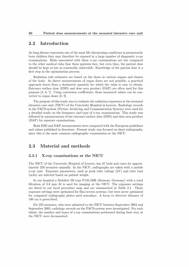
Sixty ESD measurements were performed for the chest radiograph. In this group,the average patient weight was 1.9 kg and the median ESD was 34 µGy (3-101 µGy).This is well below the EC reference dose [25] of 80 µGy for neonates of 1.0 kg andwell below the EC reference dose of 135 µGy for babies 10 months old. Table 2.2shows the results of a European dose survey for children younger than 1 year.
The median ESD was 28 µGy for the extremely low birth weight infants, 33µGy for the low birth weight infants and 52 µGyfor the normal birth weight infants

2.5 Conclusion 23
0200400600800
1000120014001600
Chest
Rad.
Babyg
ram
Abd. R
ad.
CT-Bra
in
CT-Tho
rax
Heart
Chat.
Other
Nu
mb
er o
f ex
amin
atio
ns
Figure 2.2: Overview of the number of x-ray examinations performed at the NICU.
(Table 2.3).
The median DAP-value was 0.71 cGy.cm2 (0.35 - 3.24 cGy.cm2) which is alsolower compared to the results of a European dose survey for children younger than 1year (Table 2.4) [26]. For DAP-measurements, no EC reference doses are available.
We noticed a large spread in our limited data set of measured DAP-values.Looking at the exposure settings given in 2.1, we should expect the DAP to increasewith increasing weight. However, DAP does not only depend on dose but is alsoinfluenced by the irradiated area. For 4 patients field sizes were measured for chestexaminations during 3 successive days. Normally the field size should be as smallas possible, according to the European guidelines [25]. However, Table 2.5 showsthat the field size differs from day to day. For example, looking at patient 1, thefield size is almost doubled from day 1 to day 2.
Large field sizes are linked with poor or inappropriate collimation (Figure 2.3).This is not in agreement with the ALARA-principle. Bad collimation gives rise toan unnecessarily high patient dose and deteriorates the image quality.
2.5 Conclusion
Entrance surface doses are found to be below the European reference dose of 80µGy for the chest radiograph [25]. Compared to the other medical risks that thesepatients face, the radiation risks associated with these x-ray examinations are low.However, we do not know if the radiation exposures are as low as reasonably achiev-able. Exposure parameters given in Table 2.1 were optimized for screen film systems,
24 Patient dose measurements at the neonatal intensive care unit
µGy Reported ValueCenter 1 62 (73) Median (75th perc)Center 2 77 (88) Median (75th perc)Center 3 105Center 4 79 MedianCenter 5 73 (102) Median (75th perc)Center 6 210 (90) Mean (stdev)Center 7 353 MedianCenter 8 41 MedianDRL 131Eur. Ref. Levels [25] 135
Table 2.2: ESD-values (µGy) with backscatter for chest radiography in Europeancenters for children younger than 1 year. A DRL could be calculated from these dataand can be compared to the European reference levels. (75th perc: 75th percentile;stdev: standard deviation) [26].
.
Weight (g) Median ESD (µGy) RangeExtremely low birth weight infants < 1000 28 21-34Low birth weight infants 1000− 2500 33 3-75Normal birth weight infants > 2500 52 26-101
Table 2.3: Entrance surface dose measurements (ESD) for different weight classes..
µGy Reported ValueCenter 1 1.1 (1.5) Median (75th perc)Center 4 1.7Center 6 (’99-’05) 11 (5) Mean (stdev)Center 6 (’05) 1.4 MeanCenter 7 38.6 MeanCenter 9 2.3 MeanDRL 8.8
Table 2.4: DAP-values (cGy.cm2) for chest radiography in European centers forchildren younger than 1 year. A DRL could be calculated from these data. (75th
perc: 75th percentile; stdev: standard deviation) [26]..

2.5 Conclusion 25
Field size Patient 1 Patient 2 Patient 3 Patient 4 Patient 5Day 1 56.0 cm2 90.4 cm2 189.6 cm2 189.6 cm2 89.7 cm2
Day 2 91.5 cm2 139.8 cm2 112.3 cm2 112.3 cm2 108.2 cm2
Day 3 83.8 cm2 122.2 cm2 122.2 cm2 109.2 cm2 \
Table 2.5: Field size for 4 patients for successive examinations..
Figure 2.3: Example of good collimation (left), example of bad collimation (right).
and not for computed radiography systems used nowadays. Further investigation isneeded.
Inappropriate field size is the most important mistake in pediatric radiographictechnique. A field which is too large will not only impair the image contrast and res-olution by increasing the amount of scattered radiation but also -most importantly-result in unnecessary irradiation of the body. However, correct beam limitationrequires proper knowledge of the external anatomical landmarks by the technician.This illustrates the need for both theoretical and practical teaching of the techni-cians.
In Belgium there are 19 recognized Neonatal Intensive Care Units and with thisstudy information about dose is only available for 1 center. The European studyshowed that dose variations between different centers can be large, we thereforethink it is necessary to investigate the patient doses in the other Belgian NICU’s.

Chapter 3
Calculation of organ doses inradiographic examinations ofpremature babies
Part of this work was published in:
• Smans K, Tapiovaara M, Cannie M, Struelens L, Vanhavere F, Smet M,Bosmans H,“Calculation of organ doses in x-ray examination of prematurebabies.” Med. Phys. 35(2), 556-68, (2008).
3.1 Abstract
To calculate doses in the entire body and in specific organs, computational modelsof the human anatomy are needed. Using medical imaging techniques, voxel phan-toms have been developed to achieve a representation as close as possible to theanatomical properties. In this study two voxel phantoms, representing prematurelyborn babies, were created from CT- and MRI-images: Phantom 1 (1910 g) andPhantom 2 (590 g). The two voxel phantoms were used in Monte Carlo calculations(MCNPX) to assess organ doses. The results were compared with the commerciallyavailable software package PCXMC in which the available mathematical phantomscan be downsized towards the prematurely born baby. The simple phantom-scalingmethod used in PCXMC seems to be sufficient to calculate doses for organs withinthe radiation field. However, one should be careful in specifying the irradiation ge-ometry. Doses in organs that are wholly or partially outside the primary radiationfield depend critically on the irradiation conditions and the phantom model.
26

3.2 Introduction 27
3.2 Introduction
Lung diseases represent one of the most life threatening conditions in prematurelyborn children. In the evaluation of the neonatal chest, the primary and most im-portant diagnostic study is the chest radiograph. Since prematurely born childrenare very sensitive to radiation, those radiographs may lead to a significant radiationdetriment. Knowledge of the radiation dose is therefore necessary to justify theexposures.
Radiation risk estimates are based on the doses in various organs and tissues ofthe body. In practice, direct measurement of the organ doses is not possible andtherefore organ doses must be estimated otherwise: presently they are most oftencalculated by means of Monte Carlo simulations.
The Monte Carlo method is a numerical method simulating radiation transport.It is distinguished from other simulation methods by being stochastic and usingrandom numbers. In medical physics the Monte Carlo method is used, for example,to simulate photon transport and interactions in an x-ray examination. Compu-tational models of the human anatomy are then needed to calculate doses in theentire body and in specific organs.
The first computational phantoms were equation-based stylized phantoms, whereorgans are delineated by combining simple surface equations such as for planes, el-liptical cones, ellipsoids and cylinders. This type of phantom has been referenced byvarious names such as MIRD, ORNL, mathematical, or the Cristy−Eckerman phan-tom [27, 28, 29]. Over the years, phantoms representing human beings of variousages have been developed.
Computer programs for effective dose calculations, such as PCXMC [30], areoften based on these basic phantoms. Mathematical phantoms resemble the humananatomy only roughly. More realistic human phantoms have become available basedon medical imaging techniques, such as computed tomography (CT) or magneticresonance imaging (MRI). The obtained high resolution cross-sectional digital im-ages of internal anatomy are then used to create a three-dimensional representationof the shape, volume and composition of the human organs. These so called voxelphantoms provide a more realistic representation of the anatomical structures [31].
While much effort has been devoted towards the creation of adult phantoms,only few research studies have proposed phantoms for pediatric radiology. We areaware of eight voxel phantoms that have been developed to represent pediatricpatients [32, 33, 34, 35, 36, 37, 38]. Five of them represent babies less than 1 yearold (Table 3.1). These five phantoms include one from GSF in Germany (BABY)[32, 33] and four from the University of Florida (UF Newborn, UF 2 month, UF 9month and UFH-NURBS) [34, 35, 36, 37].
BABY was constructed from 142 CT slices with a thickness of 4 mm of an 8-week female cadaver. The UF Newborn-female and UF 2-month-male phantomswere both created via image segmentation of cadavers, and represent high resolu-tion images of pediatric subjects with 485 1 mm slices and 438 1.25 mm slices,respectively. The UF 9-month-male phantom was created from fused images taken

28Calculation of organ doses in radiographic examinations of premature
babies
from head and chest-abdomen-pelvis CT examinations of the same individual. Theresolution of the phantom for the 9-month was 0.43 x 0.43 x 3.0 mm3.
From the UF Newborn a hybrid newborn phantom was developed [37]. A totalof 126 anatomical organ and tissue models are described within the hybrid phantomusing either Non-uniform rational B-Spline (NURBS) surfaces or polygon surfaces.Table 3.1 gives an overview of the baby phantoms.
Phantom Gender Weight Age Voxel size Modality[kg] [mm3 ]
BABY [32] F 4.2 2 months 2.9 CTUF newborn F 3.8 6 days 0.35 CT(original) [34]UF 2 month [34] M 5.4 2 months 0.30 CTUF 9 month [36] M 6.9 9 months 0.56 CTUFH-NURBS [37] M/F 3.5 6 days (surfaces) CT
Table 3.1: Overview of voxel phantoms representing children younger than 1 yearold.
.
These phantoms are not appropriate to represent prematurely born infants witha birth weight that can be as low as 500 g [39]. As far as we know, specific voxelphantoms for premature babies have not been presented earlier. Neither mathemat-ical phantoms have been adjusted to resemble prematurely born babies. However,PCXMC offers the ability to modify mathematical phantoms based on the patientsweight (m) and height (h). Based on these body size measurements the newbornphantom model can be downsized towards the prematurely born baby.
The purpose of the present study was to create appropriate selected voxel phan-toms for calculation of organ doses from x-ray examinations of premature babies.Furthermore, we wanted to investigate if the scaling method used in PCXMC isappropriate for dose calculations in prematurely born babies. To validate the useof PCXMC for such calculations, organ dose conversion coefficients are compared.
The development of a voxel phantom in this age group was considered a firststep towards optimisation studies in the neonatal unit. MCNPX is not limited tocalculating organ doses, but can also be used to assess image quality. In furtherwork, the voxel phantoms will be used to link patient dosimetry and image quality.
3.3 Material and methods
3.3.1 Voxel phantoms
Most voxel phantoms are based on CT-images. CT-images are particularly usefulfor segmenting bone, because of the high contrast between bone and soft tissue.
3.3 Material and methods 29
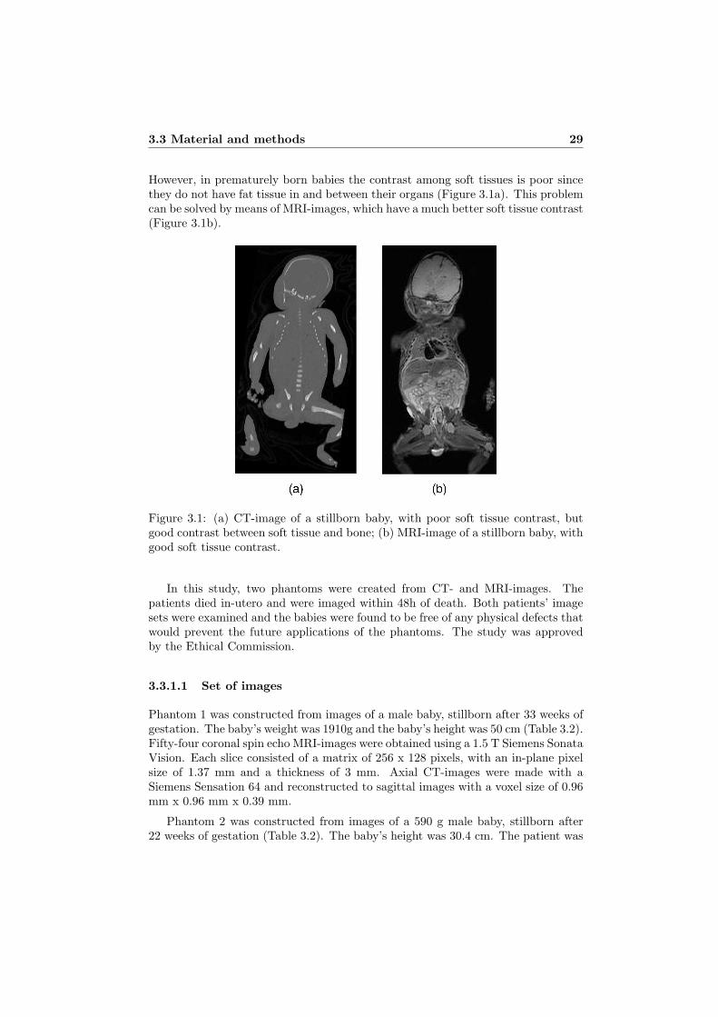
However, in prematurely born babies the contrast among soft tissues is poor sincethey do not have fat tissue in and between their organs (Figure 3.1a). This problemcan be solved by means of MRI-images, which have a much better soft tissue contrast(Figure 3.1b).
Figure 3.1: (a) CT-image of a stillborn baby, with poor soft tissue contrast, butgood contrast between soft tissue and bone; (b) MRI-image of a stillborn baby, withgood soft tissue contrast.
In this study, two phantoms were created from CT- and MRI-images. Thepatients died in-utero and were imaged within 48h of death. Both patients’ imagesets were examined and the babies were found to be free of any physical defects thatwould prevent the future applications of the phantoms. The study was approvedby the Ethical Commission.
3.3.1.1 Set of images
Phantom 1 was constructed from images of a male baby, stillborn after 33 weeks ofgestation. The baby’s weight was 1910g and the baby’s height was 50 cm (Table 3.2).Fifty-four coronal spin echo MRI-images were obtained using a 1.5 T Siemens SonataVision. Each slice consisted of a matrix of 256 x 128 pixels, with an in-plane pixelsize of 1.37 mm and a thickness of 3 mm. Axial CT-images were made with aSiemens Sensation 64 and reconstructed to sagittal images with a voxel size of 0.96mm x 0.96 mm x 0.39 mm.
Phantom 2 was constructed from images of a 590 g male baby, stillborn after22 weeks of gestation (Table 3.2). The baby’s height was 30.4 cm. The patient was

30Calculation of organ doses in radiographic examinations of premature
babies
imaged with the 1.5 T Siemens Sonata Vision. Twenty-three 3 mm coronal imageswere saved as a matrix of 256 x 104 pixels, with an in-plane pixel size of 1.2 mm.Axial CT-images were obtained using a Siemens Sensation 64 and reconstructed tosagittal images with a voxel size of 0.30 mm x 0.30 mm x 1 mm.
Phantom 1 Phantom 2Gestational Age 33 weeks 22 weeksWeight 1910 g 590 gHeight 50 cm 30.4 cmGender Male Male
Table 3.2: Patient specific properties of the two stillborn babies used for the devel-opment of the voxel phantoms.
.
The heights of Phantom 1 and Phantom 2 were measured on the CT-images.Since the legs were not straightened, we acquired the total height as the sum of thelength from skull to pelvis, the length of the upper legs and the length of the lowerlegs.
3.3.1.2 Registration
An essential prerequisite to use both CT- and MRI-images is the alignment of theimages. This requires a 3D geometric operation, which is called image-registration.The images were registered using a non-rigid registration with a B-spline transfor-mation model (rigid registration was not possible since the head moved between theCT- and MRI-examination). Because images of different modalities are registered,mutual information was chosen as similarity criterion [40].
The MRI-images were first interpolated to match the pixel size of the CT-images.For Phantom 1, the final set of images consisted of 95 coronal slices of 1-mm thick-ness and 0.96 mm x 0.96 mm in-plane resolution. For Phantom 2 the final set ofimages consisted of 73 coronal slices. The voxel size of this final set of images was1 x 0.74 x 0.74 mm3. The voxel volume for the two phantoms was 0.922 mm3 and0.548 mm3 respectively (Table 3.3).
Phantom 1 Phantom 2Matrix size 512 x 512 x 512 177 x 407 x 73Voxel size 1 x 0.96 x 0.96 mm3 1 x 0.74 x 0.74 mm3
Voxel volume 0.922 mm3 0.548 mm3
Table 3.3: Voxel dimensions of the fused image sets to create the two voxel phan-toms.
.

3.3 Material and methods 31
3.3.1.3 Segmentation
The registered and resized images were segmented into different organs. Duringthis step of the study, every voxel had to be assigned to the appropriate organ. Aspecific tissue composition was then attributed to each organ. Materials used wereNewborn Soft Tissue (1.04 g/mm3), Newborn Skeleton (1.22 g/mm3) and NewbornLung (0.296 g/mm3) [27].
The segmentation was performed with MeVisLab [19]. The segmentation ofbone could be done automatically, because of the good contrast between bone andsoft tissue in the CT-images. Soft tissues were segmented semi-automatically basedon the soft-tissue contrast in the MRI-scans. Manual segmentation corrections werenecessary for some tissues. A radiologist supervised the segmentation. The followingradiosensitive anatomic regions were segmented: testes, the major alimentary tract(stomach, small intestine, colon), lung, bladder, liver, thyroid, gonads, skin, boneand some remainder tissues (thymus, heart, brain, kidneys, pancreas, adrenals,spleen). Because the patients died in utero, the lungs were not fully inflated. Weassumed that the filling of the total thorax space with lung tissue would be a goodapproximation for the in-vivo anatomy. The esophagus could not be segmentedsince it was not visible in the images. It was created and inserted at a best-estimatelocation, without interfering with other organs. As the dimensions of bone marrowcavities (100-3000 µm) are smaller than the linear voxel dimension, bone marrowcould not be segmented either. The equivalent dose in the RBM had to be derivedfrom the energy deposited in the tissue mixture of skeletal voxels.
The skin represented another challenge. The reference skin thickness given byCristy and Eckerman [27] is 0.7 mm for a newborn. Considering the voxel dimen-sions of the two phantoms, it was decided that the outer layer voxels would beappropriate to represent the skin. This approach yielded for Phantom 1 a skinthickness of 1 mm in the antero-posterior direction and a skin thickness of 0.96 mmin the lateral direction. For Phantom 2 the skin thickness is respectively 1 mm inthe antero-posterior direction and 0.74 mm on the lateral direction.
3.3.1.4 Organ masses
The masses of all soft tissue organs were calculated as the product of the number ofsegmented voxels defining the organ, the voxel volume and the tissue density. Forboth phantoms, organ masses were compared with ICRP-reference. In ICRP 89[41] reference values are published based on measurements performed at differentgestational ages in embryos and prematurely delivered infants. ICRP 89 [41] offersfetal growth curves for the lung, kidneys, brain, heart, spleen, thymus, thyroid,adrenals, pancreas and active marrow. Using those growth curves reference ICRP-values were estimated for premature babies with the same weight as the phantoms.Next, the total mass of each of the two phantoms was calculated and comparedwith the real mass of the babies.

32Calculation of organ doses in radiographic examinations of premature
babies
3.3.2 MCNP-calculations
Monte Carlo calculations of organ doses were performed with the MCNPX version2.5.0 software package [10]. To use the newly created phantoms in MCNPX, the seg-mented images have been converted to an input file for MCNPX with Scan2MCNP[42]. The input file contains only the geometry and materials of the phantom. Aphoton source was added to simulate the x-ray beam. To simulate a clinical relevantspectrum, we used a source with a constant potential tube voltage of 65 kVp anda total filtration equivalent to 4 mm of aluminum. This spectrum was generatedwith the IPEM spectrum generator software [43]. Organ doses were calculated withMCNP’s F6 tallies, which estimate the energy deposition in the voxel.
3.3.2.1 Skeletal dosimetry
The skeleton of the phantoms was modeled as a homogenous mixture of mineralbone, active bone marrow, and other organic constituents of the skeleton. We usedthe mixture, specific for newborns, with a density of 1.22 g/cm3 [27] (Table 3.4).Table 3.4 also shows the elemental composition of red bone marrow [44].
Bone mixture Red bone marrowH 8 10.5C 9.71 41.4N 2.71 3.4O 66.8 43.9Na 0.314Mg 0.143P 3.71 0.1S 0.314 0.2Cl 0.14 0.2K 0.148 0.2Ca 8Fe 0.008 0.1
Table 3.4: Elemental composition (percentage by mass) of the bone mixture andred bone marrow.
.
For the calculation of dose in the RBM, we followed the procedure recommendedby Kramer et al [45]. The energy deposited (EDEP) by a photon in the bone mixturewas multiplied by three correction factors: F1 the fraction of RBM mass in the boneor bone group (i) where the interaction took place to the total mass of this boneor bone group, F2 the ratio between the mass-energy absorption coefficients for theRBM and the average bone mixture and F3 the King-Spiers correction factor for theadditional RBM dose from photoelectrons released in bone adjacent to the marrow

3.3 Material and methods 33
cavities [46].
EDEPRBM (i) = EDEPBoneMixture(i) · F1(i) · F2 · F3(i) (3.1)
To calculate the mass fraction of RBM in the bone, F1(i), we assumed thatthe total mass of RBM varies linearly with the total mass of the baby [41]. Fora newborn baby with a total mass of 3500g [41], the reference values for massesof active (red) and inactive bone marrow are respectively 50g and 0g [41]. Forthe distribution of RBM over the various bone groups we used the data of ICRP70 [47] (Table 3.5). These data are based on research performed by Hudson [28],who determined the volume of bone marrow in 16 fetuses (10 females and 6 males)ranging in age from 29 weeks to full term. Of the fetal bone marrow volume, 29.5%± 4.2% was found in the skull, 23.4% ± 2.5% in the trunk, and 47.1% ± 3.1% inthe limbs. These data are the same as Cristy’s recommended values for newborns[48].
Mass Fraction ICRP 70(40 weeks)
Ribcage 12.7%Spine 14.2%Skull 29.5%Pelvis 9.2%Upper Leg 7.4%Lower Leg 8.0%Feet 8.3%Upper Arm 4.6%Lower Arm 2.5%Hand 3.6%
Table 3.5: The distribution of active bone marrow in individual bones or bonegroups, expressed as the percentage of active bone marrow in the body accordingto ICRP 70 [47].
.
The mass energy absorption coefficients, needed for F2, were calculated fromthe elemental compositions for RBM and bone mixture given in Table 3.4 and theelemental mass energy absorption coefficients [44]. Since the size of the bone marrowcavities may vary depending on the age or the anatomical part of the skeleton, theKing-Spiers correction factor, F3(i), is determined for each type of bone. We usedthe King-Spiers correction factor for children 1.7 years old, the youngest age forwhich the King-Spiers correction factor is listed in [46].
The energy dependence of F2 and F3 was considered in the MCNPX calculationsby using DE/DF cards which allow to multiply the dose contribution of each particlewith an energy-dependent dose function.

34Calculation of organ doses in radiographic examinations of premature
babies
To calculate the energy deposited in the skeletal part of the bone the energydeposited in the bone marrow, EDEPRBM (i) , is subtracted from the energy de-posited in the bone mixture, EDEPBoneMixture(i).
EDEPSkeletalPart(i) = EDEPBoneMixture(i)− EDEPRBM (i) (3.2)
The dose in the RBM and skeletal part of the bone are finally calculated bydividing the EDEP by the mass:
DRBM =ΣEDEPRBM (i)
ΣMRBM (i)(3.3)
DSkeletalPart =ΣEDEPSkeletalPart(i)
ΣMSkeletalPart(i)(3.4)
With
MSkeletalPart(i) = MBoneMixture(i)−MRBM (i) (3.5)
3.3.3 PCXMC-calculations
PCXMC is an easy to use, commercially available computer program for calculatingpatient organ doses in medical x-ray examinations. The phantoms used in PCXMCare slightly modified mathematical hermaphrodite phantoms of Cristy [28] repre-senting humans of various ages: newborn, 1, 5, 10, 15-year-old, and adult. PCXMCenables further modification of these phantoms by allowing the user to change theirweight (m) and height (h). Based on these body size measurements, the programcalculates vertical and horizontal scaling factors, and modifies the phantom size andshape. The materials used in PCXMC are skeleton (1.49 g/cm3), lung tissue (0.296g/cm3) and soft tissue (0.99 g/cm3).
The composition and density of the lung tissue are similar to the compositionand density of the tissue used in the voxel phantom. The density of the soft tissueis a little higher in the voxel phantom (1.04 g/cm3 versus 0.99 g/cm3). The skele-tal densities are significantly different; PCXMC uses the skeletal tissue for adults,whereas we use skeletal tissue which is specific for newborns.
3.3.3.1 Skeletal dosimetry
In a similar way, the bones of the phantoms are modeled as a homogenous mixtureof mineral bone, active bone marrow, and other organic constituents of the skeleton.For the calculation of the RBM absorbed dose PCXMC follows a similar approachas described above, but the dose-increasing effect of bone marrow being located insmall cavities in trabecular bone [49], is approximated by using a photon energy-dependent kerma-to-dose conversion factor that is equal in all parts of the skeleton

3.3 Material and methods 35
and all phantoms. The size variation of the bone marrow cavities with patient ageor the anatomical part of the skeleton has not been taken into account in PCXMC.In our MCNPX calculations, the site-specific King-Spiers correction factors of ayoung child were used. The dose in the skeletal part of the bone is calculated in asimilar way as for the voxel phantoms.
In order to compare both computational methods, we adjusted the PCXMCnewborn phantom to match our phantoms (Phantom 1:m = 1910 g, h= 50 cm andPhantom 2:m= 590 g, h=30.4 cm).
3.3.4 Comparison
To compare the voxel phantoms and the mathematical phantoms, we simulatedx-ray beam examinations. In the simulations, we used a source with a constantpotential tube voltage of 65 kVp and a total filtration equivalent to 4 mm of alu-minum. The source-skin distance (SSD) was 105 cm. We used the incident airKerma (Ka,I) as an input dose quantity for both MCNPX and PCXMC. A totalbody antero-posterio (AP) irradiation was simulated to calculate conversion coeffi-cients (CCorgan) between organ doses (Dorgan) and Ka,I :
CCorgan =Dorgan
Ka,I(3.6)
Since in these irradiation conditions all organs are situated completely in the ra-diation field, the results mainly reflect the similarity of organ depths. We comparedthe absorbed doses in 19 organs obtained with both computational approaches. Thetwo methods are compared in a Bland Altman plot [50]. Differences were expressedin terms of the percentage:
DMCNPX −DPCXMC
DPCXMC(3.7)
In addition, a detailed analysis of the dose in the different skeletal parts wasperformed. Moreover, effective dose was calculated based on the ICRP 60 [3].
Afterwards, clinical relevant radiation fields were placed to simulate chest ra-diography (AP projection). We used the same field size for both MCNPX andPCXMC. The field size was 9.6 cm x 8 cm for Phantom 1 and 7 cm x 5 cm forPhantom 2. The position of the radiation fields was visualized with radiographytallies in MCNPX (Figure 3.2). For PCXMC the radiation fields were shown in thecomputer program itself (Figure 3.3). To investigate the influence of the field sizeand the field position, we made the radiation field for Phantom 2, 1 cm larger (7cm x 6 cm), 1 cm smaller (7 cm x 4 cm) and we moved the radiation field 1 cmtowards the head and 1 cm towards the feet.

36Calculation of organ doses in radiographic examinations of premature
babies
Figure 3.2: Position of the radiation fields in MCNPX calculations for a chestradiography. (a) Phantom 1 with field size of 9.6 cm x 8 cm; (b) Phantom 2 withfield size of 7 cm x 5 cm.
Figure 3.3: Position of the radiation fields in PCXMC calculations for a chestradiography. (a) Phantom 1 with field size of 9.6 cm x 8 cm; (b) Phantom 2 withfield size of 7 cm x 5 cm.
3.4 Results
Segmentation was performed successfully and is shown in Figure 3.4 and in Fig-ure 3.5. Not all organs are shown in order to maintain perceptible figures. Figure 3.4shows the skin, skeleton, lungs, heart, kidneys and colon for Phantom 1. For Phan-tom 2 the skin, skeleton, lungs, thymus, kidneys, adrenals and large intestine areshown in Figure 3.5.

3.4 Results 37
Figure 3.4: Three-dimensional reconstruction of Phantom 1 (1910 g; 32.6 weeksgestational age). (a) Frontal view of the phantom exterior; (b) Frontal view oflungs, heart, kidneys, colon, skeleton; (c) Frontal view of the skeletal system.
3.4.1 Organ masses
The organ masses of the two voxel phantoms are given in Table 3.6 and in Table 3.7.When an ICRP 89 reference value is available [41], a percent difference is reported.The ICRP reference values were estimated from the growth curves [41]. Variationsrange from -55% (lung; Phantom 2) to +170% (spleen; Phantom 2). For bothphantoms a close match for the kidneys, heart and adrenals is achieved. Patient-specific variations from reference masses are noted for the brain, thyroid, thymus,pancreas and lungs. For the lungs, different tissue density can explain the systematicunderestimation of the organ mass. Therefore we compared the lung volume (73.8mL Phantom 1 and 19.3 mL Phantom 2) with values published in literature [51](69 mL and 24 mL respectively).
The organ masses for the mathematical phantoms used in PCXMC are alsoshown in Table 3.6 and in Table 3.7. Organ masses are linearly scaled based onthe phantom’s total weight. There is no correction for the relatively large head andrelatively small lower limbs of the prematurely born baby.
The mass of the skin is much lower for the mathematical phantoms. In PCXMCthe skin thickness is also scaled which makes the skin thinner.
There is also a good correspondence between the total mass of the segmentedphantoms, 2009 g and 541g respectively, and the real mass of the stillborn babies,1910g and 590g respectively. Table 3.8 shows the mass of the RBM in the bone orbone groups. We also notice that there is a good agreement between the RBM masspredicted by the ICRP and the values calculated based on the phantoms weight.

38Calculation of organ doses in radiographic examinations of premature
babies
Phan
tom1
Phan
tom2
MC
NP
XIC
RP
PC
XM
CM
CN
PX
ICR
PP
XC
MC
(voxel)(refernce)
(math)
(voxel)(reference)
(math)
Organ
sTestes
0.70.4
0.20.1
Colon
16.99.5
4.217
(-55%)
2.9Lung
21.941
(-46%)
27.57.8
8.5Stom
ach2.2
3.31.6
1.0B
ladder1.0
1.50.51
23.1(18%
)0.5
Liver
67.970.8
(-4%)
62.627.3
0.2(-9%
)19.3
Thyroid
0.30.7
(-53%)
0.70.2
0.2Skin
124.160.9
49.34.6
(-25%)
18.8K
idneys14.5
14.5(0%
)11.8
3.574.5
(41%)
3.7B
rain258.7
221(29%
)181.7
105.23.7
(-15%)
56.1H
eart14.5
11(32%
)13.1
3.10.5
(167%)
4.1Spleen
6.13.4
(81%)
4.71.4
1.9(-24%
)1.5
Thym
us3.7
6.6(-44%
)5.8
1.41.2
(20%)
1.8A
drenals2.1
3.3(-35%
)3.0
1.42.5
(-49%)
0.9Pancreas
2.23.9
(-43%)
1.41.3
0.4Sm
allintestine
30.927.3
5.58.4
Esophagus
0.91.8
0.40.5
Table
3.6:O
rganand
tissuem
assesfor
thevoxel
phantoms
andthe
scaledP
CX
MC
phantoms.
When
anIC
RP
89reference
valueis
available[41],
apercent
differencew
iththe
voxelphantom
organm
assis
reported.T
heIC
RP
referencevalues
were
estimated
fromthe
growth
curves[41]:
Part
1..

3.4 Results 39
Phan
tom
1P
han
tom
2M
CN
PX
ICR
PP
CX
MC
MC
NP
XIC
RP
PX
CM
C(v
oxel
)(r
efer
ence
)(m
ath)
(vox
el)
(ref
eren
ce)
(mat
h)B
one
mix
ture
Tot
alm
ass
139.
823
2.2
56.4
71.9
Skul
l61
.745
.226
.114
.0Sp
ine
20.1
40.4
6.6
12.5
Rib
cage
20.7
27.5
8.4
8.5
Pel
vis
6.1
23.3
2.2
7.2
Arm
s12
.436
.75.
711
.3U
pper
Arm
s5.
22.
5L
ower
Arm
s4.
32.
1H
and
Wri
sts
2.9
1.1
Leg
s18
.849
.67.
515
.3U
pper
Leg
s9.
63.
8L
ower
Leg
s6.
62.
9F
eet
Ank
les
2.6
0.8
Tot
al20
0919
1019
1054
159
059
0
Tab
le3.
7:O
rgan
and
tiss
uem
asse
sfo
rth
evo
xelph
anto
ms
and
the
scal
edP
CX
MC
phan
tom
s.W
hen
anIC
RP
89re
fere
nce
valu
eis
avai
labl
e[4
1],
ape
rcen
tdi
ffere
nce
wit
hth
evo
xel
phan
tom
orga
nm
ass
isre
port
ed.
The
ICR
Pre
fere
nce
valu
esw
ere
esti
mat
edfr
omth
egr
owth
curv
es[4
1]:
Par
t2
.

40Calculation of organ doses in radiographic examinations of premature
babies
Figure 3.5: Three dimensional reconstruction of Phantom 2 (590 g; 22 weeks ges-tational age). (a) Frontal view of the phantom exterior; (b) Frontal view of lungs,kidneys, adrenals, colon, gonads, skeleton; (c) Frontal view of the skeletal system.
3.4.1.1 Total body irradiation
The results of the total body irradiation are presented in Table 3.9. In MCNPX,5 · 107 particles left the source, which resulted in stochastic errors less than 1%(for all organs). In PCXMC the number of particle histories was 2 · 106 and thestochastic errors were less than 1% for organs in the radiation field, and typicallyless than 7% for low dose organs.
The Bland-Altman plot [50] is a statistical test to compare two measurementtechniques. In this graphical method, the differences between the MCNPX andPCXMC conversion coefficients are plotted against the averages of the two tech-niques (Figure 3.6). The plot shows that there is no systematic difference betweenMCNPX and PCXMC for Phantom 2 as a function of the magnitude of organ doseconversion coefficients. For Phantom 1 there is a small systematic difference: 0.06mGy/mGy. The differences within mean 1.96 SD are 0.46 mGy/mGy for Phantom1 and 0.33 mGy/mGy for Phantom 2. The correlation coefficient between the con-version coefficients calculated with MCNPX and PCXMC is R=0.84 for Phantom1 and R=0.87 for Phantom 2.
For relatively superficial organs close to the beam, such as liver, heart and pan-creas, there is a good agreement between the voxel phantoms (MCNPX) and themathematical phantoms (PCXMC). For organs at the posterior side, the conversion

3.4 Results 41
Phantom 1 Phantom 2MCNPX ICRP PCXMC MCNPX ICRP PXCMC(voxel) (ref) (math) (voxel) (ref) (math)
RBMTotal mass 25.6 27 25.6 7.9 8.4 7.9Skull 7.6 2.3Spine 3.6 1.1Ribcage 3.3 1.0Pelvis 2.4 0.7Arms 2.7 0.9 Upper Arms 1.2 0.4 Lower Arms 0.6 0.2 Hand Wrists 0.9 0.3Legs 6.0 1.9 Upper Legs 1.9 0.6 Lower Legs 2.0 0.6 Feet Ankles 2.1 0.7
Table 3.8: Red Bone Marrow (RBM) mass in individual bones or bone groups forthe voxel phantoms. The ICRP reference for the total RBM mass was estimatedusing the ICRP 89 growth curves [41]. Total RBM mass is also given for the scaledPCXMC phantoms.
.
coefficients for the voxel phantoms (MCNPX) are larger than the conversion coeffi-cients for the mathematical phantoms (PCXMC). Looking at effective dose, we seea remarkably good agreement for the total body examination.
Table 3.10 shows the RBM dose conversion coefficients calculated for the voxelphantoms (MCNPX). The PCXMC software package does not provide the RBMconversion coefficients separately for the individual bone groups. Only one con-version coefficient is given for the total RBM: 0.49 mGy/mGy for Phantom 1 and0.57 mGy/mGy for Phantom 2. There are relatively small differences between theconversion coefficients between the two voxel phantoms.
Conversion factors for the bone were also calculated for the different bone groupsand compared with the mathematical phantoms of PCXMC (Table 3.11). There isa good correspondence for skull and the whole skeleton. For the spine and pelvisthe conversion coefficients are lower for the mathematical phantoms.
3.4.1.2 Chest radiography
Table 3.12 shows the conversion coefficients for the simulations of chest radiography.We compared the organ doses based on their position with respect to the radiation

42Calculation of organ doses in radiographic examinations of premature
babies
CC Phantom 1 Phantom 2[mGy/mGy] MCNPX PCXMC Rel. MCNPX PCXMC Rel.
(voxel) (math) Diff. (voxel) (math) Diff.Testes 1.12 1.43 -22% 1.01 1.36 -26%Colon 0.87 0.82 11% 1.02 0.90 14%Lung 0.83 1.01 -18% 0.78 1.04 -25%Stomach 0.99 0.92 8% 0.94 0.97 -3%Bladder 0.64 1.15 -45% 1.13 1.23 -8%Liver 1.25 1.01 24% 0.98 1.05 -7%Thyroid 0.90 0.85 6% 0.88 0.88 0%Skin 0.64 0.38 69% 0.64 0.48 33%Kidneys 0.65 0.53 24% 0.68 0.63 7%Brain 0.70 0.39 79% 0.77 0.50 53%Heart 0.78 0.71 10% 0.76 0.79 -5%Spleen 1.02 0.81 26% 0.97 0.87 11%Thymus 1.11 0.84 31% 0.97 0.91 6%Adrenals 0.65 0.55 18% 0.75 0.65 15%Pancreas 1.01 1.13 -11% 0.99 1.14 -13%SmallIntestine 0.98 0.96 2% 0.96 1.01 -6%Esophagus 0.87 0.57 30% 0.91 0.66 38%Eff. Dose 0.87 0.88 -1% 0.84 0.95 -11%
Table 3.9: Conversion coefficients (mGy/mGy), expressed as mean organ dose(mGy) per incident air Kerma, Ka,I , (mGy) for a total body irradiation. Source-Skin-Distance: 105 cm, 65 kVp, total filtration: 4 mm Al, Direction: antero-posterior.
.
field (Figure 3.2 and Figure 3.3).
For organs within the radiation field the relative differences in conversion coef-ficients are small, and range from -13% for the thymus in Phantom 2 to 16% forthe lungs in Phantom 1. Table 3.13 shows that for organs within the radiation field(lungs and heart) the position and size of the radiation field do not have a largeinfluence on the conversion coefficients. For organs partially in the radiation field(liver and spleen) the relative differences in conversion coefficients are large. InPCXMC the radiation field is restricted to the lung, heart and thymus (Figure 3.3).Due to the realistic shape of the lungs in the voxel phantoms, the liver, stomach,esophagus and spleen are partially included in the radiation field (Figure 3.2). ForPhantom 1 even parts of the pancreas and adrenals are included in the field. Forthese organs, we see that the difference in conversion coefficients for the voxel phan-toms compared to the doses for the mathematical phantoms range from 26% for

3.4 Results 43
CC Phantom 1 Phantom 2[mGy/mGy] (voxel) (voxel)Ribcage 0.71 0.79Spine 0.51 0.67Skull 0.77 0.80Pelvis 0.74 0.75Upper Legs 0.75 0.83Lower Legs 0.81 0.82Feet 0.78 0.86Upper Arms 0.88 0.88Lower Arms 0.84 0.94Hands 0.90 0.85Total RBM 0.74 0.79
Table 3.10: Conversion coefficients (mGy/mGy) for the RBM in individual bones orbone groups for the voxel phantoms. Conversion coefficients are expressed as meanorgan dose (mGy) per incident air Kerma, Ka,I , (mGy) for a total body irradiation.Source-Skin-Distance: 105 cm, 65 kVp, total filtration: 4 mm Al, Direction: antero-posterior.
.
CC Phantom 1 Phantom 2[mGy/mGy] MCNPX PCXMC Rel. MCNPX PCXMC Rel.
(voxel) (math) Diff. (voxel) (math) Diff.Skull 2.14 2.12 1% 2.27 2.44 -7%Spine 1.76 1.07 65% 2.28 1.44 59%Ribcage 2.39 2.78 -14% 2.55 2.98 -14%Arms 3.17 2.34 36% 2.95 2.66 11%Legs 3.18 2.32 37% 2.97 2.65 12%Pelvis 3.14 1.60 96% 2.89 1.98 46%Skeleton 2.35 2.20 7% 2.49 2.55 -2%RBM 0.74 0.49 50% 0.79 0.57 39%
Table 3.11: Conversion coefficients (mGy/mGy) for the individual bones or bonegroups for the voxel phantoms and the mathematical phantoms. Conversion co-efficients are expressed as mean organ dose (mGy) per incident air Kerma, Ka,I ,(mGy) for a total body irradiation. Source-Skin-Distance: 105 cm, 65 kVp, totalfiltration: 4 mm Al, Direction: antero-posterior.
.

44Calculation of organ doses in radiographic examinations of premature
babies
CC Phantom 1 Phantom 2[mGy/mGy] MCNPX PCXMC Rel. MCNPX PCXMC Rel.
(voxel) (math) Diff. (voxel) (math) Diff.Within field
Lung 0.83 0.71 16% 0.95 0.81 18%Heart 0.90 0.86 4% 0.89 0.91 -2%Thymus 0.93 1.02 -9% 0.93 1.06 -13%
Partially within fieldLiver 0.66 0.15 340% 0.28 0.19 50%Stomach 0.68 0.09 710% 0.22 0.11 95%Spleen 0.39 0.08 400% 0.47 0.10 360%Esophagus 0.58 0.36 61% 0.54 0.43 26%Pancreas 0.51 0.08 510%Adrenals 0.47 0.11 310%
Partially within fieldPancreas 0.08 0.08 -4%Adrenals 0.06 0.17 -61%Kidneys 0.09 0.03 210% 0.02 0.04 -46%Thyroid 0.09 0.08 12 % 0.09 0.09 5%SmallIntestine 0.06 0.01 660% 0.02 0.01 53%Colon 0.05 0.01 640% 0.01 0.01 -4%Bladder 0.01 0.00 230% 0.00 0.00 -12%Brain 0.01 0.00 640% 0.01 0.00 190%Testes 0.00 0.00 NA 0.00 0.00 -40%
Widely distributed tissuesSkin 0.13 0.14 -7% 0.15 0.15 -2%Bone 0.45 0.40 9% 0.50 0.48 1%RBM 0.11 0.07 52% 0.13 0.09 47%Eff. Dose 0.30 0.21 38% 0.22 0.24 -11%
Table 3.12: Conversion coefficients (mGy/mGy), expressed as mean organ dose(mGy) per incident air Kerma, Ka,I , (mGy) for a chest radiograph. Source-Skin-Distance: 105 cm, 65 kVp, total filtration: 4 mm Al, Direction: antero-posterior.
.

3.4 Results 45
Figure 3.6: Bland-Altman plot presenting the difference between the conversion co-efficients calculated with MCNPX and PCXMC against the average of the MCNPXand PCXMC conversion coefficients. (a) Phantom 1, (b) Phantom 2.
the esophagus (Phantom 2) up to 710% for the stomach (Phantom 1).
These large differences result from the difference of the fraction of organs thatare located in the primary beam. Table 3.13 shows that the conversion coefficients

46Calculation of organ doses in radiographic examinations of premature
babies
of the partly irradiated organs, such as liver and spleen, are extremely sensitive tothe collimation and location of the beam: for example, if the beam location is moved1 cm towards the feet, the conversion coefficient for the dose in the liver increasesfrom 0.28 mGy/mGy to 0.56 mGy/mGy for the voxel phantom (MCNPX) and from0.19 mGy/mGy to 0.51 mGy/mGy for the mathematical phantom (PCXMC). Therelative difference between the voxel and mathematical phantom decreases from50% to 10%. Shifting the beam 1 cm towards the head the conversion coefficients ofthe liver decrease to 0.05 mGy/mGy for MCNPX and 0.04 mGy/mGy for PCXMC.
CC [mGy/mGy] 7× 5 7× 6 7× 4 Down UpLung MCNPX 0.95 0.98 0.93 0.96 0.86
PCXMC 0.81 0.83 0.76 0.78 0.66Heart MCNPX 0.89 0.91 0.86 0.82 0.82
PCXMC 0.91 0.94 0.88 0.93 0.74Liver MCNPX 0.28 0.44 0.14 0.56 0.05
PCXMC 0.19 0.36 0.05 0.51 0.04Spleen MCNPX 0.47 0.64 0.29 0.68 0.07
PCXMC 0.10 0.25 0.05 0.40 0.04
Table 3.13: Conversion coefficients (mGy/mGy) for the RBM in individual bones orbone groups for the voxel phantoms. Conversion coefficients are expressed as meanorgan dose (mGy) per incident air Kerma, Ka,I , (mGy) for a total body irradiation.Source-Skin-Distance: 105 cm, 65 kVp, total filtration: 4 mm Al, Direction: antero-posterior.
.
Therefore, it is seen that the comparison of doses in partially irradiated organs isnot straightforward. Even large differences in the results do not necessarily depictincompatibility of the results between the different calculation models. Similardeviations would be unavoidable also in comparing different voxel models.
For organs outside the primary beam the conversion coefficients are small (<0.1 mGy/mGy) compared to organs within the radiation field. For these organs,the relative differences in organ dose can also be high (640% for the small intestineof Phantom 1), however the absolute differences are small.
For widely distributed body organs such as skin, bone and RBM the relativedifferences in conversion coefficients range from -7% for the skin of Phantom 2 upto 52% for the RBM of Phantom 1. For the effective dose, there is a fair agreementbetween MCNPX and PCXMC; the relative differences in conversion coefficientsrange from -11% for Phantom 2 (both total body irradiation and chest radiograph)up to 38% for Phantom 1 (chest radiograph).
To calculate organ doses the conversion coefficients need to be multiplied withthe Ka,I . If we use the clinical exposure settings used in our hospital, the lungdose for a chest x-ray calculated with MCNPX was 23.7 µGy (Ka,I : 30 µGy) forPhantom 1 and 16.0 µGy (Ka,I : 18 µGy) for Phantom 2. With PCXMC the results

3.5 Discussion 47
are respectively 21.4 µGy for Phantom 1 and 14.5 µGy for Phantom 2.
The effective dose, calculated with MCNPX and its hermaphrodite phantommodel, results in 9 µSv (Ka,I : 30 µGy) and 4.0 µSv (Ka,I : 18 µGy) for phantom1 and 2, respectively, whereas calculated with PCXMC the results are respectively6.3 µSv and 4.3 µSv.
3.5 Discussion
The purpose of present study was to create realistic voxel phantoms for calculation oforgans doses from x-ray examinations of prematurely born babies. The phantomscreated in this work represent only two cases of premature babies, with a verydifferent gestational age. Organ dose conversion coefficients, calculated using thevoxel phantoms, were compared with the results from the PCXMC program.
For the standard hermaphrodite phantoms (newborn, 1, 5, 10, 15-year-old, andadult patients), organ dose conversion factors calculated with PCXMC have beenvalidated with data available from NRPB [52, 53]. However, the adjustable pediatricphantoms of the PCXMC, and more in particular the extreme case of the verysmall premature baby, have not been validated before. Therefore, the comparisonsin this study can also be partly considered to validate the use of PCXMC for suchcalculations. We noticed that the linear scaling method used in PCXMC does notaccurately model the relatively large head of prematurely born babies. The mass ofthe brain and skull are underestimated compared with the ICRP reference valuesand the values from the voxel phantoms. The organ masses of the voxel phantoms donot fully adhere to ICRP 89 reference values of organ masses in all cases. However,other authors reported similar deviations in organ masses caused by anatomicaldifferences [35, 45].
The total body irradiation calculations showed close agreement between dosecalculations with the voxel phantoms and with the mathematical phantoms (Fig-ure 3.6). In general, we see that for organs at the posterior side the dose conversioncoefficients for the voxel phantoms (MCNPX) are higher compared to the mathe-matical phantoms (PCXMC). This is not unexpected, considering the differencesin the phantom shapes. The PA-thickness for the voxel models is 65 mm for Phan-tom 1 and 50 mm for Phantom 2 and for the mathematical models respectively 73mm and 52 mm. The PA-thicknesses for the voxel models were measured on axialCT-images of the thorax.
For organs at the posterior side there will be less shielding by overlying tissue inthe voxel models. Small differences in organ depths may result in significant dosedifferences: MCNPX calculations show about 20% dose reduction per 1 cm depth,and even more in the lateral direction for an x-ray beam with a peak tube voltage65 kVp and a filtration of 4 mm Al.
The differences in skeletal dosimetry are mainly caused by anatomical differencesbetween the mathematical and voxel phantom. The influence of skeletal density(1.22 g/cm3 (voxel) versus 1.49 g/cm3 (mathematical)) is rather small. In a similar

48Calculation of organ doses in radiographic examinations of premature
babies
way as for organs at the posterior side, the conversion coefficients for the spine arehigher for the voxel phantoms because there is less shielding by overlying tissue. Forthe pelvis, this effect is reinforced by a difference in anatomical shape of the pelvis(Figure 3.7). This may be contrasted with the dose to the ribs, which is actuallyhigher for the mathematical phantom. The reason for this is illustrated in Figure 3.7which compares the skeletons in the two phantom model types: the front part of theribs is still cartilage in both premature babies and the voxel phantoms, whereas inthe mathematical phantom the ribs are fully formed. Despite the fact that the skullis too small in the mathematical phantoms, there is reasonable agreement betweenthe two phantoms for doses to the bones of the skull.
Figure 3.7: Frontal view of the skeletal system for Phantom 2 (590 g; 22 weeksgestational age): (a) voxel phantom, (b) mathematical phantom. The anatomicalshape of the pelvis and ribs are different for the two phantoms.
We know that, due to the anatomical model differences, the dose in the variousbones may differ notably in the voxel and mathematical phantoms. This has a directconsequence on the RBM dose, which is systematically lower for the mathematicalphantoms compared to the voxel phantoms. Moreover, the distribution of the RBMhas an influence on the RBM dose. There is not too much information about theRBM distribution in preterm babies. For fetuses ICRP 70 [47] provides tables withthe distribution of RBM over the various bone groups. According to ICRP 70 [47]29.5% of the fetal RBM is present in the skull, 23.5% in the trunk and 41.7% in thelimbs.

3.5 Discussion 49
A more recent study performed by Wilpshaar [54] showed a very different dis-tribution for children born after 16 - 22 weeks of gestation, namely that the largestcomponent of the total bone marrow was the spine, which constituted 26.4% (Ta-ble 3.14). The skull contained only 6.7%, which is due to the absence of hematopoi-etic cells in the calvarial bones (skull). According to Wilpshaar [54], bone marrowcells could only be detected after 22 weeks of gestation.
Mass Fraction ICRP 70 Wilpshaar(40 weeks) (16 - 22 weeks)
Ribcage 12.7% 12.3%Spine 14.2% 26.4%Skull 29.5% 6.7%Pelvis 9.2% 9.5%Upper Leg 7.4% 14.1%Lower Leg 8.0% 9.4%Feet 8.3% 0.8%Upper Arm 4.6 % 8.8%Lower Arm 2.5% 5.4%Hand 3.6% 2.3%
Table 3.14: The distribution of active bone marrow in individual bones or bonegroups, expressed as the percentage of active bone marrow in the body accordingto ICRP 70 [47] and Wilpshaar [54].
.
In present study, we have used the fetal RBM distribution provided by the ICRP70 [47]. However, for our models this RBM distribution may not be appropriate.The proportions of the bone marrow do not reflect the relatively large head andsmall lower limbs in premature babies. In the mathematical newborn model and thescaled PCXMC-models, 20% of the skeleton mass is situated in the legs, whereas inour voxel models the legs comprises 13% of the skeletal mass. According to ICRP70 [47] 23.7% of the fetal RBM is present in the legs, resulting in relative highfractions of RBM in bone for the voxel phantoms.
The skin dose mainly results from the energy absorbed in the skin in the pri-mary beam. We notice that, despite the different shape and skin thickness of thephantoms, there is a good agreement in skin dose.
For chest radiography, the differences in conversion coefficients for organs withinthe radiation field range from -13% (thymus phantom 2) to 16% (lung phantom 1).Similar differences are reported by other authors comparing voxel phantoms andmathematical phantoms [35, 45]. Differences in shapes, sizes and locations of theorgans are the major causes for the dose differences. For organs partly in theradiation field there is a large influence of the position and size of the radiationfield. Small changes in field position and size can result to dose differences ofseveral hundred percent. There is no fair way in placing x-ray fields ”similarly” in

50Calculation of organ doses in radiographic examinations of premature
babies
two different phantoms in order to compare doses in organs that are partly in theprimary beam.
To estimate radiation risk, the ICRP [3] has introduced effective dose (E). Theeffective dose is a weighted sum of the doses in a large number of radiation sensitiveorgans and tissues. In the definition of the effective dose the tissue weighting factorshave been developed from a reference population of equal numbers of both sexesand a wide range of ages. Their relevance for a different population, e.g. as is in thispaper, is not known and the use of effective dose in describing doses in diagnosticradiology has been criticized [55, 56]. Moreover, the effective dose is sex-averagedand is to be applied only to reference individuals. The two voxel phantoms describedhere are both male and do not fully adhere to ICRP 89 reference values of organmasses in all cases. Therefore, in this paper we have only listed the calculated organdoses which will be used in future patient dosimetry.
For a chest radiograph the doses are typically low. For example, in our hospitalthe lung dose in a 2 kg (Ka,I : 30 µGy) premature baby who is exposed to theaverage of 10 chest radiographs is of the order of 250 µGy. Even if 80 radiographsare required, dose to the lung will be approximately 2 mSv.
The present study will be followed by a clinically related study that investigatesthe quality of the radiographic image and a technical study that investigates whetherthe optimal beam quality is chosen. MCNPX is not limited to calculating organdoses, by using radiography tallies also image quality can be evaluated. In ourfurther work, the two voxel phantoms presented here will link patient dosimetryand image quality.
3.6 Conclusion
The phantoms described in this study are useful for calculating conversion factorsfrom Ka,I to organ doses. For organs within the radiation field the doses calculatedwith the voxel phantoms correlated well with doses calculated with the PCXMCprogram. Therefore, the simple phantom-scaling method used in PCXMC wouldalso seem to be sufficient for these purposes. However, one should note that therewill be considerable uncertainty on doses to organs that are partly or totally out-side the radiation field, because the actual primary beam location in the patientand patient anatomy cannot be exactly reproduced in simulations. As expecteddifferences in skeletal structure and RBM/bone distributions between the phantommodels developed here and those specified in PCXMC give rise to variations in boneand RBM dose conversion factors. The new premature baby phantoms described inthis study will undergo further refinement and elaboration as a tool to investigatex-ray beam quality optimisation.

Chapter 4
Radiographic imagesimulation with the MonteCarlo software packageMCNP/MCNPX
Part of this work is submitted for publication in:
• Smans K, Carton A-K, Verbrugge B, Haeck W, Struelens L, VanhavereF, Bosmans H,“Radiographic image simulation with Monte Carlo softwareMCNP/MCNPX.” submitted for publication in Medical Physics at 07/05/09.
4.1 Abstract
Radiographic image simulation based on Monte Carlo techniques allows the user toevaluate and optimize a variety of aspects in the imaging chain such as x-ray spec-tra, system geometries, acquisition parameters and radiation dose. MCNP/MCNPXdeveloped the radiographic tally for simulation of radiographic images. The radio-graphic tally, used in image simulation studies previously published, calculates thespatial distribution of primary and scattered radiation using a grid of closely spacedF5 point detectors. The purpose of presented technical note is to show the radio-graphic tally does not accurately compute the spatial distribution of primary andscattered x-rays and therefore can not be correctly applied in image simulationstudies. In addition, we present two alternative methods to accurately assess thecontribution of primary and scattered radiation in a time-effective way. Validationswere performed using the scatter-to-primary ratio (SPR). SPR results for the threeMonte Carlo methods were compared against both published results and experimen-tally acquired SPR values. It was found that SPRs computed with the radiographic
51

52Radiographic image simulation with the Monte Carlo software package
MCNP/MCNPX
tally are 21% (1% - 46%) larger on average than both published and experimen-tally acquired values, while SPRs computed with the two proposed methods arerespectively 1% (-5% - 2%) and 0.1% (-5% - 5%) smaller on average than publishedand experimentally acquired values. Above results suggest that our methods canbe used correctly for the evaluation of radiographic imaging techniques.
4.2 Introduction
MCNP/MCNPX [10] is a general-purpose Monte Carlo code for simulating radia-tion transport that is developed and owned by Los Alamos National Laboratory.MCNP/MCNPX was originally developed to simulate nuclear processes, such asfission and fusion. Today, its use has expanded to other scientific fields includinghigh-energy physics, medical physics, and space sciences.
Medical physics, and more specifically diagnostic radiology, differs from its nu-clear counterpart by using photons with energy up to 150 keV. To describe thephoton transport in this low energy range, a specific photon physics treatment isconsidered. All photon physical processes taking place at the considered energies,e.g. photoelectric absorption, incoherent (Compton) and coherent (Thomson) scat-tering, fluorescence emission, have to be taken into account.
In diagnostic radiology, Monte Carlo techniques have been widely used to cal-culate doses in the entire body as well as in specific organs. However, Monte Carlotechniques are not limited to calculating organ doses, but can also be used to sim-ulate x-ray images. While much effort has been devoted towards the calculation ofscatter fractions [57, 58, 59], only few research studies have focused so far on imagesimulation studies for realistic pixel sizes (100 µm) [60, 61, 62].
Radiographic image simulation can be obtained implementing different detectormodels. In a previous image simulation study by Kyprianou [62] a perfect energyintegrating detector was used. This detector model, also used in scatter studiesby Boone [57] and Sechopoulos [58], assumed 100% efficiency for absorbing x-rayphotons. A more dedicated detector model computing the energy absorbed by thedetector from each incident x-ray was presented in an image simulation study byPeplow [60]. This detector model includes the spectral sensitivity of the detectormaterial.
Whereas for mammographic applications (with a photon energy up to 38 keV)where low energy photon beams are almost completely absorbed by the detectormaterial, the perfect energy integrating detector model is a good approximation;detector models taking into account the spectral sensitivity of the detector material,should be used for general radiography applications (photon energy up to 150 keV)[11]. MCNP/MCNPX offers a predefined detector model, the radiography tallywhich, according to the manual, can be used to generate radiographic images [10].This radiography tally was used previously in image simulation studies [63, 64, 65]and is based on point detector techniques.
In this paper we will show that the radiography tally overestimates the con-

4.3 Theory 53
tribution of scattered radiation. Therefore we present two alternative methods tosimulate high resolution images with MCNP/MCNPX within a reasonable comput-ing time. Simulations are performed for the perfect energy integrating detector andfor a photostimulable phosphor as x-ray detection material. Validation is done bycomparison of calculated scatter-to-primary ratios (SPRs) against results publishedin literature and experimentally acquired results. The SPR is defined as the totalscattered x-ray photon energy absorbed by the detector and divided by the totalprimary x-ray photon energy absorbed by the detector.
4.3 Theory
In MCNP/MCNPX, tallies are specified by the type of information the user wantsto gain from the Monte Carlo calculation. Tally cards are denoted by the characterF followed by a number indicating the tally type. All tallies are calculated usingthe particle weight W which is a number carried along by each particle, representingthat particle’s relative contribution to the final results.
MCNP/MCNPX offers a predefined detector tally, the radiography tally (MCNP:FIR or ∗FIR; MCNPX: TIR or ∗TIR), which is a grid of closely spaced F5 pointdetector tallies forming an image detector. F5 point detectors are used to calculatea semi-deterministic estimate of the fluence at a specific point. For all particles leav-ing the source (source event) and every time a particle undergoes a collision (scatterevent) the contribution to the tally is calculated using the ray-trace technique asdescribed by the Lambert-Beer law:
F5 =p(Ωp)R2
·W · e∫ R0 −∑
t(s)ds (4.1)
With W the particle weight, p(Ωp) the probability density function which de-scribes the probability that a particle will scatter towards the point detector (direc-tion Ωp), R the distance between source/scatter event and the point detector, and−∑
t(s) the total macroscopic cross section at a distance from the source or colli-sion point to the point detector. The term e
∫ R0 −∑
t(s)ds describes the probabilitythat a particle has a collision-free flight for the distance R to the detector point.
Since contributions to the point detector are made at every source and scatterevent separately, point detectors can discriminate between primary and scatteredradiation. Moreover, due to its semi-deterministic nature, the radiography tally isfast and high resolution images (100 µm) for both the source and scatter events canbe obtained in a short time.
For photons, MCNP/MCNPX offers five more standard tallies: current (F1),fluence (F2 and F4) and dose (F6, ∗F8 and +F8). An overview of all tallies, except∗F8 and +F8, is given in Table 4.1. If the F card is flagged with an asterisk (∗F ),the tally score will be multiplied with the particle energy E.
The tally surface and tally volume are shown in Figure 4.1

54Radiographic image simulation with the Monte Carlo software package
MCNP/MCNPX
CurrentF1 Surface current Stochastic, summed for all[Particles] F1 = ΣW particle tracks crossing the[MeV ] F1 = ΣW · E detector surface A
FlueneF2 Surface fluence Stochastic, summed for all[Particles] F2 = Σ W
A·| cos α| particle tracks crossing the[MeV ] F2 = Σ W ·E
A·| cos α| detector surface A
F4 Track length estimate Stochastic, summed for all[Particles] F2 = ΣW ·TL
V particle tracks crossing the[MeV ] F2 = ΣW ·TL·E
V detector surface A
F5 Point Detector Semi-deterministic[Particles] F5 = p(Ωp)
R2 ·W · e∫ R0 −∑
t(s)ds calculated for every[MeV ] F5 = p(Ωp)
R2 ·W · E · e∫ R0 −∑
t(s)ds source and scatter eventDose
F1 Surface current Stochastic, summed for all[MeV ] F6 = ΣW ·TL
V · σt ·H particle tracks crossing thedetector surface A
Table 4.1: Standard photon tallies used in MCNP/MCNPX. W = particle weight,E = particle energy, α = incident angle between the particle trajectory and thenormal on the surface (MCNP/MCNPX sets | cos α| = 0.05 when | cos α| < 0.1), TL = track length, C = collision site, σt = total atomic cross-section and H =photon heating numbers which estimates the energy deposited per unit track length.
.
Figure 4.1: The tally surface (left) and tally volume (right).
Except for the semi-deterministic F5 tally (Figure 4.2a) all tallies described inTable 4.1 are stochastic (Figure 4.2b). For stochastic tallies, particles will onlycontribute to the tally score if they effectively reach the detector element (the sur-

4.3 Theory 55
face or volume defined to calculate the tallies). In order for this to happen, theparticle must scatter towards the detector element. This occurs with a probability:∫Ωp
p(ΩpdΩp, with p(Ωp) the probability density function which describes the prob-ability that a particle will scatter in the direction of the detector element and Ωp
the solid angle subtended by the detector element (Figure 4.2b). The larger Ωp, thelarger the probability that the particle will effectively reach the detector element.For a pixel sized detector element, as is being used in radiology, the solid angle Ωp
can be approximated by (Figure 4.2d):
Ωp ≈ | cos α| ·AR2
(4.2)
with R the distance between the particle and the detector element and α theincident angle between the particle trajectory and the normal on surface A. Fig-ure 4.2d shows two particles at identical distance R from the detector element. Dueto the cosine factor in equation 4.2, the probability that particles leaving point 1(α = 0o) will be directed towards the detector will therefore be larger compared toparticles leaving point 2 (α > 0o).
The semi-deterministic F5 point detector, using the ray-trace method, has nosuch angular sensitivity, but assumes that particles leaving point 1 and particlesleaving point 2 have the same probability to be detected by the point detector ifscatter material and distance R are identical (Figure 4.2c).
This is illustrated in Figure 4.3. A pixel sized detector element (100 µm x100 µm) was exposed to an isotropic point source and placed in a scatter freeenvironment. The distance from the source to the detector was 1 m. To investigatethe angular sensitivity described above, we changed the incident angle between theparticle trajectories and the normal on the detector surface. Since the source-to-detector distance was 1 m, α could be considered constant over the 100 µm x 100 µmdetector surface. We tallied F1 that is counting the number of particles crossing thedetector surface A, and F5. The F5 point detector was placed in the center of thedetector surface used to calculate F1. Figure 4.3 shows the number of particles perunit of area. We observe that F1
A is decreasing with | cos(α)|, whereas F5 remainsconstant. This shows that F5 overestimates the number of particles reaching thepixel sized detector surface by 1
| cos(α)| :
F5 =F1
A · | cos(α)| (4.3)
The same relation is valid for the flagged tallies:
∗F5 =∗F1
A · | cos(α)| (4.4)
Figure 4.4 shows the geometry of a typical imaging system used in general radi-ology. For primary radiation the incident angle α between the particle trajectoriesand the normal on a pixel sized detector surface (100 µm x 100 µm) is very small.
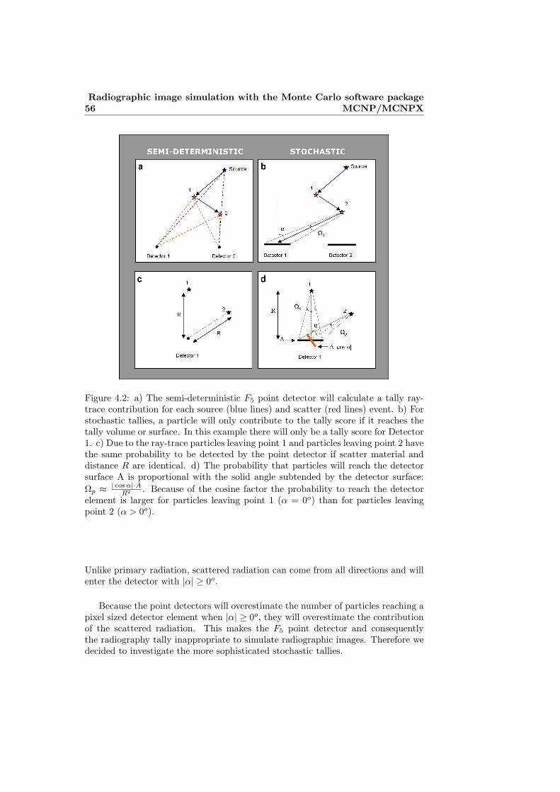
56Radiographic image simulation with the Monte Carlo software package
MCNP/MCNPX
Figure 4.2: a) The semi-deterministic F5 point detector will calculate a tally ray-trace contribution for each source (blue lines) and scatter (red lines) event. b) Forstochastic tallies, a particle will only contribute to the tally score if it reaches thetally volume or surface. In this example there will only be a tally score for Detector1. c) Due to the ray-trace particles leaving point 1 and particles leaving point 2 havethe same probability to be detected by the point detector if scatter material anddistance R are identical. d) The probability that particles will reach the detectorsurface A is proportional with the solid angle subtended by the detector surface:Ωp ≈ | cos α|·A
R2 . Because of the cosine factor the probability to reach the detectorelement is larger for particles leaving point 1 (α = 0o) than for particles leavingpoint 2 (α > 0o).
Unlike primary radiation, scattered radiation can come from all directions and willenter the detector with |α| ≥ 0o.
Because the point detectors will overestimate the number of particles reaching apixel sized detector element when |α| ≥ 0o, they will overestimate the contributionof the scattered radiation. This makes the F5 point detector and consequentlythe radiography tally inappropriate to simulate radiographic images. Therefore wedecided to investigate the more sophisticated stochastic tallies.

4.4 Material and methods 57
Figure 4.3: F1A calculated for a pixel sized detector element (100 µm x 100 µm)
exposed to an isotropic point source and placed in a scatter free environment. Thesource detector distance was 1m. The F5 point detector was placed in the center ofthe detector surface used to calculate F1. In this experiment α is the incident anglebetween the particle trajectory and the normal on the pixel sized detector surface.
Figure 4.4: In radiology the incident angle α between the particle trajectories andthe normal on a pixel sized detector element is very small and can be consideredconstant for primary radiation. Unlike primary radiation, scattered beam can orig-inated from all directions and will often enter the detector with |α| ≥ 0o. Primaryradiation is presented by the solid lines and scattered radiation is presented by thered dotted lines.
4.4 Material and methods
In this study we present two alternative methods to simulate images in MCNP /MCNPX. Using the more sophisticated stochastic tallies described in Table 4.1 wemodeled two x-ray detectors with typical pixel sizes of digital imaging detectors.The first detector (detector 1) was assumed to have 100% efficiency for absorbingx-ray photons. The second detector (detector 2) consisted of a phosphor plate as is

58Radiographic image simulation with the Monte Carlo software package
MCNP/MCNPX
used in computed radiography (CR) systems.
However, image simulation for realistic pixel sizes (100 µm) using stochasticMonte Carlo techniques would require prohibitively long computing times. To re-duce the calculation time larger pixel sizes can be used but all clinically relevantdetails such as small lesions may be lost. Therefore, a balance between resolutionand calculation time needs to be found.
Based on the scatter point spread function calculated by Boone [57] we canconclude that the scattered image does not show small structures (Figure 4.5) .Therefore pixel sizes of 5 mm, also used by Peplow et al [60], were deemed smallenough for appropriate characterization of x-ray scatter variation with position. Byincreasing the pixel size from 100 µm x 100 µm to 0.5 cm x 0.5 cm, calculation timeis reduced by a factor 2500.
Figure 4.5: Scatter image not showing small structures (left) and accompanyingprimary image showing small details (right).
As described by the Lambert-Beer law primary images which require the highresolution from x-ray detectors (100 µm) can be calculated using ray-trace tech-niques. Since for those images no full Monte Carlo simulation is needed, highresolution images can be obtained in a very short calculation time.
This inspired us to calculate the scattered and primary image separately. Toconstruct the total image, the low resolution scattered image will be interpolatedand added to the high resolution primary image.
In MCNP/MCNPX, the deterministic F5 and ∗F5 point detectors are the onlytallies which offer the possibility to calculate the primary and the scattered contribu-tion separately. A more general way to discriminate between primary and scatteredradiation can be obtained by using the surface source write/surface source read-cycle (SSW/SSR) features in MCNP/MCNPX. In a first calculation, the surfacesource write (SSW) cycle allows the user to carry out the radiation transport upto a certain surface, and record all particle tracks in a file. For tracks crossing thissurface, the relevant information (such as position, energy and direction) is stored.In a second calculation, this information will be used in the surface source read(SSR) cycle, where the transport of the particle tracks crossing the surface will becontinued. Using the collision option flag in the SSR command (primary: COL=1,scatter: COL=-1), it is possible to distinguish between particles that came directly

4.4 Material and methods 59
from the source without a collision and particles that had collisions before crossingthe recording surface. To prevent extra scatter events between the SSW/SSR sur-face and the detector surface, the SSW/SSR plane was placed as close as possible (inpractice 0.01 mm) above the detector surface. This way primary- and scatter-onlyimages can be generated separately.
4.4.1 Perfect energy integrating detector
The first detector was modeled as a perfect energy integrating detector. A perfectenergy integrating detector assumes 100% efficiency for absorbing x-ray photons,regardless of their energy and angles of incidence. To model a detector with thosespecifications in MCNP/MCNPX, we used a grid of ∗F1 current tallies. The ∗F1
tally counts the number of particles crossing the detector surface and multiplies thetally score with the particle energy E: ∗F1 = ΣW · E.
A scatter only image was generated using the SSW/SSR cycle with the colli-sion option flag. The grid was defined using the repeated structure tally card andwas programmed to have a 5 mm resolution. This was deemed small enough forappropriate characterization of x-ray scatter variation with position, but still largeenough to obtain reasonable statistics.
To generate the high resolution primary image, we used the radiography tally(MCNP: ∗FIR; MCNPX:∗TIR) equipped with semi-deterministic ∗F5 point de-tectors. Using this tally, a ray-trace contribution was calculated for all particlesleaving the source. From the previous section we know that point detectors willoverestimate the number of particles reaching a pixel sized detector element (100µm x 100 µm) by 1
| cos α| with α the incident angle between the primary beam andthe normal on the detector surface (Figure 4.2). Since α can be calculated based onthe position of the source and the detector pixel, ∗F5 tallies can be converted intothe ∗F1 tallies used to model a perfect energy integrating detector:
∗F1 =∗ F5 · | cos(α)| ·A (4.5)
To form the total image, the low resolution scattered image will be interpolatedand added to the high resolution primary image.
4.4.2 Photostimulable phosphor
The second detector was modeled as a photostimulable phosphor imaging plate.In a similar way as reported by Jing et al [59], the actual energy absorbed bythe phosphor from each incident x-ray photon was computed. In a photostimulablephosphor the energy absorbed is a measure of the receptor sensitivity and is directlylinked to the signal intensities in the resulting image. Unlike the perfect energyintegrating detector model, this detector model takes into account the spectralsensitivity of the detector material.

60Radiographic image simulation with the Monte Carlo software package
MCNP/MCNPX
To calculate the absorbed detector dose we used a grid of F6 dose tallies. Usingthe F6 dose tally, the Monte Carlo process continues in the detector material andwill introduce blurring due to the scatter of photons within the phosphor layer ofthe detector material. However, in a real photostimulable phosphor there will beadditional blurring introduced by optical photon transport, which is not includedin our Monte Carlo calculations. Therefore, we decided to follow an alternativeapproach based upon the fact that blurring properties of an imaging detector aredescribed by the point spread function (PSF), which presents the response of animaging detector to a point source. Since all blurring is contained in the detectors’PSF, we choose to develop a detector model without any blurring and to correctthe simulated image afterwards by convolving it with the PSF.
To turn off fluorescence and coherent scattering in the detector material the“simple physics model” [10] is used for all x-rays with energy above 1 keV (inMCNP/MCNPX: phys:p 0.001). Bremsstrahlung is turned off using the physicscard (in MCNP/MCNPX: phys:p j 1). To prevent incoherent scattering these cross-sections are changed to 0 (σincoh = 0) in the used cross-section libraries and weredirectly added to the photo-electric effect (σtot = σPE + σcoh + σincoh) so thatthe total cross-section σtot was not changed. In MCNP/MCNPX the track lengthis a stochastic quantity. A photon will travel a distance l before undergoing aninteraction [10]:
l = − 1µt· ln(ε) (4.6)
In this equation ε is a random number from [0, 1) and µt = ρ·σt
u·A , with u=1.660e−24 and A is the relative atomic mass and σt = σPE +σcoh +σincoh, the total crosssection. In reality, depending on the photon energy and cross-sections of the detec-tor material, the photon will afterwards continue its way in the detector material,generate secondary particles or it will be absorbed. In the simplified model, neitherscattering nor generation of secondary particles will occur at the collision site andthe photon is assumed to be completely absorbed by a photoelectric interaction(Figure 4.6), therefore TL = l. This simplified approximation is acceptable for adetector, because in the detector material the photoelectric effect dominates.
The absorbed energy calculated using the F6 dose tally is computed by multi-plying the track length (TL) by energy dependent cross-sections (σt) and photonheating numbers (H) (Table 4.1):
F6 = ΣW · TL
V· σt ·H (4.7)
With W the particle weight and V the detector volume.
Photon heating numbers are estimates of the energy deposited per unit tracklength. The numbers are averaged over incoherent scattering, pair production andthe photoelectric absorption:
H(E)average = E − Σ3i=1pi(E)[Ei,out(E)] (4.8)

4.4 Material and methods 61
Figure 4.6: Calculation of track length: l = − 1σt· ln(ε) with ε a random number
from [0, 1) and with σtot = σPE + σcoh + σincoh. In the simplified model the x-raywill be photo-electrically absorbed without any scattering event taking place. Thetrack length TL cannot exceed δ
| cos(α)| with δ the thickness of the detector materialand α the incident angle of a particle.
With
• i = 1 → incoherent (Compton) scattering form factors.
• i = 2 → pair production; Ei,out(E) = 2m0c2 = 1.022016 MeV
• i = 3 → photoelectric absorption; Ei,out(E) = 0 MeV
• pi(E) = probability of reaction i at gamma incident energy E
• Ei,out(E) = average exiting gamma energy for reaction i at photon incidentenergy E.
Average heating numbers H(E)average are fixed and tabulated in the librariesof MCNP/MCNPX [10]. They do not change by changing the cross-sections.
In the simplified model ΣTL will be lower since there are no tracks generatedby scattered radiation, fluorescence and bremsstrahlung and consequently so willbe the energy deposition. By convolving the simulated image with the PSF of thedetector, we mimic the physical process and get an image which is directly linkedto the signal intensities in experimentally acquired images. However, we can notcompensate for the energy loss.
To generate a scatter only image we used a grid of F6 dose tallies. The gridwas defined using the repeated structure tally card and was programmed to have a5 mm resolution, which was considered sufficient to model the scattered image. Ascatter-only image was obtained using the SSW/SSR cycle with the collision optionflag (COL=-1). Since we do not want to interfere with the radiation transport in thescattering object the options to prevent blurring in the detector material were onlyapplied in the SSR-cycle, which covers the radiation transport from the SSW/SSRsurface towards the detector.
To obtain a high resolution primary image, we used the radiography tally (MCNP:FIR or MCNPX:TIR) with its semi-deterministic F5 point detectors. In a similar

62Radiographic image simulation with the Monte Carlo software package
MCNP/MCNPX
way as described for the perfect energy integrating detector, a ray-trace contribu-tion was calculated for all particles leaving the source. Those F5 point detectortallies need to be converted to the F6 dose tallies which were used to calculatethe scattered image. If we follow a large number of particles, equation 4.8 can beapproximated by:
F6 = ΣW · TL
V· σt ·H ≈ TLΣ
W
V· σt ·H (4.9)
With TL is the average distance traveled in the detector material. In the sim-plified model without photon scattering, nor fluorescence or bremsstrahlung, theaverage track length TL in the detector material can be calculated:
TL = l =1µt
∫ 1
ε=0
ln(ε) · dε =∫ ε=A
ε=0
δ
| cos α| · dε +∫ ε=1
ε=A
− 1µt· ln(ε) · dε (4.10)
With δ the thickness of the detector element and α the incident angle betweenthe particle trajectories and the normal on a pixel sized detector element. In thisequation A ∈ [0, 1) is the random number where− 1
µt·ln(A) is the maximum distance
that can be traveled in the detector material: − 1µt· ln(A) = δ
| cos α| (Figure 4.4).This integral can be solved analytically:
TL =δ
| cosα| ·A +1µt
[1−A(1− ln(A))] (4.11)
Figure 4.7 shows TL in function of energy for a 500 µm thick CsBr:Eu2+ phos-phor plate with a surface density of 0.17 g.cm−2 and an incident angle: α = 0o.
In the previous section it was shown that for a pixel sized detector element (100µm x 100 µm) exposed to a point source and placed in a scatter free environment:
F5 =F1
A · | cos α| (4.12)
With F1 =∑
W and V = A · δ, equation 4.12 becomes:
F5 = ΣW · δ
V · | cos α| (4.13)
Combining equation 4.8 and equation 4.14 we get:
F6 ≈ F5 · σt ·H · TL · | cosα|δ
(4.14)
This way F5 tallies can be converted into the F6 dose tallies used to modela photostimulable phosphor imaging plate. Note that σt, H and TL are energy

4.4 Material and methods 63
050
100150200250300350400450500
0 20 40 60 80 100
Energy (keV)
Tra
ck L
engh
t (µm
)
Figure 4.7: TL in function of energy for a 500 µm thick CsBr:Eu2+ phosphor platewith a surface density of 0.17 g · cm−2 and an incident angle: α = 0o.
dependent. Ignoring the influence of the position of the pixels, correction can bemade within the Monte Carlo code by adding energy depended multipliers (DE/DFcards), otherwise we have to perform energy binning in the detector material andmake the corrections afterwards. Also for this detector model the low resolutionscattered image will be interpolated and added to the high resolution primary imageto create the total image.
4.4.3 Validation: comparison with literature
Monte Carlo calculations were performed with the MCNPX version 2.5.0 softwarepackage. The most recent photon libraries (MCLIB04) were selected. To validateour detector models, a series of comparisons were carried out against previouslypublished work.
A first comparison was made to the data reported by Jing et al [59]. Jing calcu-lated SPRs in a scanning slot detector geometry designed for digital mammographyusing the EGS Monte Carlo software [66]. In this paper the detector surface wasnot subdivided in pixels, but the SPRs were calculated for the entire detector ele-ment. SPRs were assessed for Lucite phantoms of various thicknesses (T), and forvarious air gaps between phantom and detector. Jing et al. performed calculationsfor two detectors. The first detector was a perfect energy integrating detector, thesecond detector consisted of a 36.7 mg/cm thick Gd2O2S:Tb phosphor as the x-raydetection material.
We mimicked SPR calculations for a 10 mm wide slot detector exposed by a
64Radiographic image simulation with the Monte Carlo software package
MCNP/MCNPX
mono-energetic 20 keV x-ray beam. We used the geometry as described by [59].SPRs were calculated using the radiography tally. Furthermore, calculations wereperformed with our model for the perfect energy integrating detector (based on ∗F1
detectors) and our model for photostimulable phosphor (based on F6 detectors).Since the SPRs were calculated for the entire detector element we integrated theprimary and scattered radiation over the entire detector surface before calculatingthe SPR.
Comparisons were also made with the work of Sechopoulos et al [58]. Sechopou-los used the Monte Carlo software Geant 4 [67] to calculate SPR maps found fortomosynthesis of the breast. In their calculations the detector was modeled to be aperfect energy integrating detector. We mimicked the SPR calculations for a breastwith a chest wall to nipple distance (CND) of 13 cm, a glandularity of 50% and withvarying breast sizes (2 cm, 5 cm and 8 cm) using Rh/Rh 31 kVp x-ray spectrum.A detailed description of the geometry can be found in [58]. Calculations were per-formed using the radiography tally (based on F5 point detectors) and our model forthe perfect energy integrating detector (based on ∗F1 detectors). The spectrum of31 kVp Rh/Rh was generated with the IPEM spectrum generating software [43].The SPR was calculated at a position through the center of mass of the breast andat 5 cm from the chest wall.
4.4.4 Validation: comparison with measurements (beam stopmethod)
The Monte Carlo calculations were also compared with experimentally assessedSPR values. The SPR was computed using the beam stop method described byCarton et al. [68]. Experiments were performed with HD 5.0 CR detectors (Agfa-HealthCare N.V., Mortsel, Belgium) and read out with a DX-S line scanning unit(Agfa-HealthCare N.V., Mortsel, Belgium). Imaging was done with a W-targetx-ray tube (Optitop 152/40/80HC, Siemens, Erlangen, Germany) with a total fil-tration equivalent to 3.8 mm Al.
Primary and scattered radiation were measured at the center of the irradiatedarea of 50 mm thick PMMA phantom positioned on top of the CR plate (air gap 5mm and without antiscatter grid). The PMMA phantom was exposed at 65 kVp.The focus-detector distance was 93 cm and experiments to calculate the SPR wereperformed for two fields of view (FOV): 10 cm x 10 cm and 30 cm x 30 cm.
In the Monte Carlo simulations the HD 5.0 CR plates were modeled as a 500 µmthick CsBr:Eu2+ phosphor plate with a surface density of 0.17 g.cm−2. We per-formed SPR calculations using the radiography tally (based on F5 point detectors),our model for the perfect energy integrating detector (based on ∗F1 detectors) andour model for photostimulable phosphor (based on F6 detectors). The spectrum(65 kVp, 3.8 mm Al filtration) was generated with the IPEM spectrum generatingsoftware [43].

4.5 Results and discussion 65
4.5 Results and discussion
4.5.1 Validation: comparison with literature
Table 4.2 shows the SPR computed for a perfect energy integrating detector. Thereis a good agreement between the results obtained with the ∗F1 tally in MCNP/MCNPX and those reported by Jing. The maximum difference between our re-sults and the ones reported by Jing [59] is 3%. As expected the radiography tallyoverestimates the SPR up to 44%.
T (cm) Air gap (cm) Jing [59] Radiography Perfect energytally integrating detector
2 3 0.06 0.06 7% 0.06 -3%1.5 0.09 0.10 11% 0.09 -1%0 0.20 0.26 30% 0.18 -1%
4 3 0.11 0.11 4% 0.10 2%1.5 0.15 0.16 7% 0.15 -2%0 0.29 0.34 17% 0.27 -2%
6 3 0.15 0.15 1% 0.14 -1%1.5 0.21 0.22 6% 0.19 -1%0 0.35 0.40 14% 0.33 1%
Table 4.2: SPR as a function of Lucite phantom thickness (T) at 20 keV x-rayenergy calculated using a 36.7 mg/cm thick Gd2O2S:Tb x-ray absorbing phosphor.Results published by Jing et al. [59] are compared with the SPR values obtainedusing the radiography tally and the model calculating the energy absorbed in thephosphor. A percent difference is reported.
.
The SPRs obtained using the absorbed energy in the detector material (36.7mg · cm2 thick Gd2O2S:Tb phosphor) are shown in Table 4.3. Also for this detectormodel there is a good agreement between our results and those published by Jing[59]. The maximum difference amounts to 5%. We see that for this detector modelthe SPR is ∼ 7% higher than that calculated when using a perfect energy integratingdetector. Using the radiography tally the SPR is overestimated up to 30%.
The SPR calculations made by Sechopoulos are compared with our Monte Carloresults in Table 4.4. The results show that varying breast thicknesses a good agree-ment between the results obtained with the ∗F1 detector and those with a perfectenergy integrating detector as used by Sechopoulos. The maximum difference be-tween the results is 2%. As was already shown for Jings experiment, we notice thatthe radiography tally overestimates the SPR up to 43%.

66Radiographic image simulation with the Monte Carlo software package
MCNP/MCNPX
T (cm) Air gap (cm) Jing Radiography Absorbed energytally in phosphor
2 3 0.06 0.06 7% 0.06 -1%1.5 0.09 0.10 11% 0.09 3%0 0.20 0.26 30% 0.19 -5%
4 3 0.11 0.11 4% 0.11 -1%1.5 0.15 0.16 7% 0.15 2%0 0.29 0.34 17% 0.28 -5%
6 3 0.15 0.15 1% 0.15 -1%1.5 0.21 0.22 6% 0.21 -1%0 0.35 0.40 14% 0.37 5%
Table 4.3: SPR as a function of Lucite phantom thickness (T) at 20 keV x-rayenergy calculated using a 36.7 mg/cm thick Gd2O2S:Tb x-ray absorbing phosphor.Results published by Jing et al. [59] are compared with the SPR values obtainedusing the radiography tally and the model calculating the energy absorbed in thephosphor. A percent difference is reported.
.
T (cm) Sechopoulos Radiography Absorbed energytally in phosphor
2 0.25 0.35 39% 0.25 2%5 0.56 0.80 43% 0.57 1%8 0.92 1.23 33% 0.92 1%
Table 4.4: SPR as a function of breast thickness measured through the center ofmass of the breast at 5 cm from the chest wall for a breast with CND 13 cm andglandularity 50%. Calculations were performed for a 31 kVp Rh/Rh; a detaileddescription of the geometry is described in [58].
.
4.5.2 Validation: comparison with measurements (beam stopmethod)
Experimentally assessed SPR values were compared with our Monte Carlo-derivedresults in Table 4.5. There is a good agreement between the experimental valuesand the F6 detector model, calculating the absorbed energy in the photostimulablephosphor. The SPRs calculated with the perfect energy integrating ∗F1 detectorsare ∼ 6% lower than those calculated using the model to calculate absorbed energyin the photostimulable phosphor. Those results are similar to the ones reported byJing. The radiography tally overestimated the measured SPR up to 46%.

4.5 Results and discussion 67
FO
V(c
m)
Mea
sure
men
tsR
adio
grap
hy
Per
fect
ener
gyA
bso
rbed
ener
gyta
lly
inte
grat
ing
det
ecto
rin
phos
phor
100.
761.
0438
%0.
73-4
%0.
782%
300.
921.
3346
%0.
87-5
%0.
91-1
%
Tab
le4.
5:SP
Ras
afu
ncti
onof
Fie
ldof
Vie
wca
lcul
ated
and
mea
sure
dfo
r5
cmP
MM
Apl
aced
onto
pof
the
HD
5.0
phot
o-st
imul
able
phos
phor
.C
alcu
lati
ons
and
mea
sure
men
tsw
ere
perf
orm
edfo
r65
kVp;
3.8
mm
Al.
.

68Radiographic image simulation with the Monte Carlo software package
MCNP/MCNPX
4.6 Conclusion
In this study we have focused on methods to simulate radiographic images withthe Monte Carlo software MCNP/MCNPX. First simulations were performed usingthe MCNP/MCNPX‘s predefined radiography tally which according to the manualcan be used to simulate radiographic images. The radiography tally calculatesthe spatial distribution of primary and scattered radiation using a grid of closelyspaced F5 point detectors. The F5 point detectors have no angular sensitivity andwill therefore overestimate the contribution of the scattered radiation.
Next to the radiography tally we also presented two alternative methods tosimulate accurate images with MCNP/MCNPX in a time effective way. Simulationswere performed for a perfect energy integrating detector and for a photostimulablephosphor.
To validate the detector models we computed scatter-to-primary ratios (SPRs)for a range of parameters of interest, which included the x-ray field of view, x-rayenergy, air gap, phantom thickness and detector composition. These parametersspan applications in mammography and conventional x-ray imaging.
As expected the SPRs calculated with the radiography tally were up to 50%higher than published and experimentally acquired values. For the two alternativemethods an excellent agreement was found between our results and data publishedin literature and experimentally measured SPRs.
Our results suggest that our methods can be used for the evaluation of radio-graphic imaging techniques, whereas the radiography tally should not be used inimage simulation studies. With this study we also want to stress that validationand understanding of the physics behind the Monte Carlo models is crucial.

Chapter 5
Validation of an imagesimulation technique for twocomputed radiographysystems used in pediatricx-ray imaging
Part of this work is submitted for publication in:
• Smans K, Carton A-K, Vandenbroucke D., Pauwels H., Struelens L, Van-havere F, Bosmans H,“Validation of an image simulation technique for twocomputed radiography systems used in pediatric x-ray imaging.” submittedfor publication in Medical Physics at 07/05/09.
5.1 Abstract
A computer model has been developed to simulate the image acquisition for twocomputed radiography (CR) imaging systems used in pediatric radiography in ourhospital. A Monte Carlo technique was used to yield realistic modeling of a pri-mary and scattered x-ray image incident on the CR detectors. This image wasmodified, using physical characteristics of the imaging system, to account for thesignal intensity variations due to the heel effect along the anode-cathode axis, thespatial resolution characteristics of the CR detectors and the various sources ofimage noise. To evaluate our computer model, a quantitative comparison was per-formed between synthetic images of a contrast-detail phantom generated with ourcomputer model and experimentally acquired images of a physical version of this
69

70Validation of an image simulation technique for two computed
radiography systems used in pediatric x-ray imaging
phantom. Typical acquisition parameters for pediatric chest x-ray examinationswere evaluated. Threshold-contrast curves were computed for the synthetic and ex-perimentally acquired images using a commercially available scoring program. Thethreshold-contrast curves of the synthetic and real images show good agreement.This implies that our computer model is able to accurately simulate the real imagingsystems. The proposed computer model is intended to be used in the optimisationof the studied imaging systems.
5.2 Introduction
Optimisation of an imaging system is necessary to balance the requirement for goodimage quality at an as low as reasonable achievable radiation dose to the patient[3]. Special attention should be given to pediatric imaging since doses accumulatedduring childhood result in an increased risk of radiation induced cancers [3].
Image quality performance of a system is often assessed using physical character-istics of the imaging system such as the noise equivalent quanta (NEQ) or detectivequantum efficiency (DQE) [69, 70, 71]. However, these objective measures pro-vide no direct link with observer performance in clinical images. Therefore, imagequality at a specific dose is also measured by the performance of an observer ona specific task. Assessment of threshold contrast detectability in images of physi-cal contrast-detail phantoms is generally proposed [70, 71, 72]. Alternatively, de-tectability studies of (simulated) lesions in images of anthropomorphic phantomsor patients are performed. While physical (anthropomorphic) phantoms provideknown ground truth, their use is limited by lack of flexibility to vary the configu-ration of the phantoms. Contrast objects or anatomical backgrounds arranged in aspecific configuration will inevitably have a great effect on the observers’ memory.As a result, perception tasks will be biased. In studies using patients the groundtruth is often unknown; it is almost impossible to know for sure whether a diseaseis present or absent in the underlying anatomical structures, unless a diagnosis isverified by physical examination or if a biopsy is performed.
Image simulation based on Monte Carlo techniques also allows to evaluate andoptimize a variety of aspects in the imaging chain such as x-ray spectra, systemgeometries, acquisition parameters and radiation dose. In addition, it allows to de-sign and evaluate new imaging systems by characterizing them by spatial resolution,noise and detection efficiency. Computer models using Monte Carlo techniques offerthe possibility to generate highly realistic synthetic images of many variations of(complex) ground truth phantoms from a specific imaging system. As a result thecomputer model gives the analyst the ability to perform experiments not possible inthe lab. As computer processing capacity has been increased, image simulation us-ing Monte Carlo techniques can nowadays be obtained in reasonable computationaltimes.
There are only a handful of studies that have used Monte Carlo techniques tosimulate images; most of the work is done in breast x-ray imaging [58, 60] and weare only aware of two studies in chest x-ray imaging [64, 73]. In the first study [60]

5.3 Material and methods 71
digital images of the ACR phantom were simulated for two different x-ray digitalmammography modalities, whereas the second study [58] used simulated imagesto investigate the acquisition parameters of tomosynthesis. The latter two [64, 73]simulate chest x-rays of an adult voxel model, without taking into account detectorproperties. As far as we know, no comprehensive Monte Carlo based simulationstudy, including characteristics of the imaging system and the detector, has beenpublished for general radiology applications.
In this study, a Monte Carlo technique was used to yield realistic modeling ofa primary and scattered x-ray image incident on the CR detectors. This imagewas modified, using physical characteristics of the imaging system, to account forthe signal intensity variations due to the heel effect along the anode-cathode axis,the spatial resolution characteristics of the CR detectors and the various sources ofimage noise.
A computer model is presented to simulate the image acquisition for two com-puted radiography (CR) imaging systems. Simulations were performed using MonteCarlo calculations and physical characteristics of the detectors. To validate our com-puter model, a quantitative comparison was performed between synthetic images ofa contrast-detail phantom generated with our model and experimentally acquiredimages of a physical version of this phantom. Typical acquisition parameters forpediatric chest x-ray imaging were evaluated. A commercially available softwareprogram was used to read the contrast-detail images and the threshold-contrastcurves were compared. It must be noted that automatic methods lead to thresholdcontrasts lower than those found by humans [15, 74]. However, the relationshipbetween computer readout and human observer scoring for the CDRAD test objecthas been explored for two systems (CR-system and a flat panel detector) [15].
5.3 Material and methods
5.3.1 Imaging systems
Two commercially available computed radiography (CR) systems used in pediatricradiography at the University Hospital of the Catholic University of Leuven (Bel-gium) were studied. The characteristics of the detectors are shown in Table 5.1.The MD 40.0 CR detectors (Agfa-HealthCare N.V., Mortsel, Belgium) were readout with an ADC Compact (Agfa-HealthCare N.V., Mortsel, Belgium); a standardflying spot scanner [75]. The two readout axes for the ADC Compact were de-fined as scan (direction of the laser beam) and subscan (direction of image platemovement) axes. The HD 5.0 CR detectors (Agfa-HealthCare N.V., Mortsel, Bel-gium) were read out with a DX-S (Agfa-HealthCare N.V., Mortsel, Belgium); aline-scanning unit [75]. The two readout axes for the DX-S were defined as the scan(direction of the CCD movement) and CCD (direction parallel to the linear CCDarray) axes. Throughout the text the acronyms MD40.0-ADC will be used to referto the MD40.0 CR detectors in combination with the ADC Compact reader andHD5.0-DX-S will be used to refer to the HD5.0 CR detectors in combination with

72Validation of an image simulation technique for two computed
radiography systems used in pediatric x-ray imaging
the DX-S reader.
Product name MD 40.0 HD 5.0Vendor Agfa AgfaComposition FBr(Sr I) Ba CsBr:Eu2+Phosphor loading 0.087 g · cm−2 0.17 g · cm−2
Phosphor packing density 70% 90%Phosphor structure Powder NeedlePixel size 170 µm 100 µmArray Size [pixel x pixel] 2048 x 2494 4200 x 3408Imaging Area [cm x cm] 35 cm x 43 cm 35 cm x 43 cmData Depth (encoding) 12 bits/pixel (sqrt) 16 bits/pixel (linear)Speed Class 200 400
Table 5.1: Characteristics of the computed radiography detectors. The MD 40.0CR detectors are readout with an ADC Compact scanner, the HD 5.0 CR detectorsare readout with an Agfa DX-S scanner.
.
The MD 40.0 and HD 5.0 CR detectors were imaged with a W-target x-ray tube(Optitop 152/40/80HC, Siemens, Erlangen, Germany). This x-ray tube has a halfvalue layer (HVL) of 2.6 mm Al at 65 kV nominal tube voltage, which results in atotal filtration of 3.8 mm Al [43]. In the standard chest x-ray protocol applied atour institution for patients in the 0.5-3.5 kg weight class, the CR plate is imaged ontop of the patient support plate without anti-scatter grid in the x-ray beam. Thedistance from the x-ray focus to the CR plate is 93 cm; the large focal spot (1 mm)and a nominal tube voltage of 65 kV are selected. A patient entrance air kerma of50 µGy is used [76].
5.3.2 Contrast-detail phantom
To compare the performance of the two CR imaging systems, threshold-contrastdetectability was assessed using a commercially available CDRAD contrast-detailphantom (Artinis Medical Systems BV, Netherlands) [13]. The CDRAD test ob-ject consists of a 10 mm thick, 265 mm x 265 mm wide polymethyl methacrylate(PMMA) support in which cylindrical holes are drilled of varying depths (0.3 - 8.0mm) and diameters (0.3 - 8.0 mm) (Figure 5.1). The holes are arranged in a 15 by15 matrix. Rows contain holes of identical diameter and exponentially increasingdepth. Columns contain holes of identical depth and exponentially decreasing di-ameter. Each square matrix element of the first three rows contains one hole in thecenter. Each square matrix element of the remaining 12 rows contains two identicalholes; one in the center and a second one randomly placed in one of the four corners.
To simulate the lung equivalent thickness of a 3.5 kg patient, twenty mm thickPMMA blocks were placed above and below the CDRAD phantom. In a separate
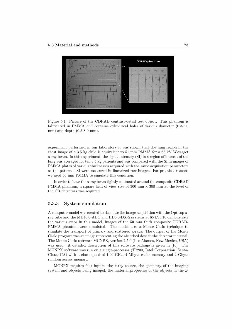
5.3 Material and methods 73
Figure 5.1: Picture of the CDRAD contrast-detail test object. This phantom isfabricated in PMMA and contains cylindrical holes of various diameter (0.3-8.0mm) and depth (0.3-8.0 mm).
experiment performed in our laboratory it was shown that the lung region in thechest image of a 3.5 kg child is equivalent to 51 mm PMMA for a 65 kV W-targetx-ray beam. In this experiment, the signal intensity (SI) in a region of interest of thelung was averaged for ten 3.5 kg patients and was compared with the SI in images ofPMMA plates of various thicknesses acquired with the same acquisition parametersas the patients. SI were measured in linearized raw images. For practical reasonswe used 50 mm PMMA to simulate this condition.
In order to have the x-ray beam tightly collimated around the composite CDRAD-PMMA phantom, a square field of view size of 300 mm x 300 mm at the level ofthe CR detectors was required.
5.3.3 System simulation
A computer model was created to simulate the image acquisition with the Optitop x-ray tube and the MD40.0-ADC and HD5.0-DX-S systems at 65 kV. To demonstratethe various steps in this model, images of the 50 mm thick composite CDRAD-PMMA phantom were simulated. The model uses a Monte Carlo technique tosimulate the transport of primary and scattered x-rays. The output of the MonteCarlo program was an image representing the absorbed dose in the detector material.The Monte Carlo software MCNPX, version 2.5.0 (Los Alamos, New Mexico, USA)was used. A detailed description of this software package is given in [10]. TheMCNPX software was run on a single-processor (T7200, Intel Corporation, Santa-Clara, CA) with a clock-speed of 1.99 GHz, 4 Mbyte cache memory and 2 Gbyterandom access memory.
MCNPX requires four inputs; the x-ray source, the geometry of the imagingsystem and objects being imaged, the material properties of the objects in the x-

74Validation of an image simulation technique for two computed
radiography systems used in pediatric x-ray imaging
ray beam and detector tallies. The x-ray source was modeled as an isotropic x-raypoint source. We used a source with a constant tube potential of 65 kVp anda total filtration of 3.8 mm Al. This x-ray spectrum was simulated by using anenergy weighted sampling of photon energies generated with the IPEM spectrumgenerator software [43]. MCNPX‘s geometry package allows to define the geometryof the x-ray system and the objects being imaged by nesting simple basic shapessuch as planes, rectangular boxes, and cylinders. The image acquisition geometrywas modeled as described in Section 5.3.1 and 5.3.2. To simulate a 300 mm x 300mm x-ray field at the detector level, a perfect radio opaque collimator of 0.32 mmx 0.32 mm at 1 mm from the point source was simulated. The materials used weredescribed by their elemental weight fraction and densities [44].
The detector was modeled as a photostimulable phosphor plate, as describedin Chapter 4. In this model the actual energy absorbed by the phosphor fromeach incident x-ray photon was computed. In a photostimulable phosphor this is ameasure of the receptor sensitivity and is directly linked to the signal intensities inthe resulting image. To reduce the calculation time a low resolution scatter imageand a high resolution primary image were calculated separately.
Since the scattered image does not show small structures, pixel sizes of 5 mm aredeemed small enough for appropriate characterization of x-ray scatter variation withposition [6]. In order to reduce the stochastic error to 1%, 109 photons generatedat the x-ray source have to be tracked. This requires 32 hours of computation time.
As described by the Lambert-Beer law, primary images, which require the highresolution from x-ray detectors, can be calculated using ray-trace techniques. Sincefor those images no full Monte Carlo simulation is needed, high resolution imagesto depict the fine details present in the phantom can be obtained in a very shortcalculation time. To simulate the HD5.0-DX-S CR detector, a 4200 x 3408 arrayof detectors with 100 µm x 100 µm mesh resolution was defined. To simulate theMD40.0-ADC CR detector, a 2048 x 2494 array of detectors with 170 µm x 170 µmmesh resolution was defined. To reduce the stochastic error in the output imageto 1%, 500 mono-chromatic x-rays were sampled from the spectrum per detectortally. The primary images for the HD5.0-DX-S and the MD40.0-ADC systems weresimulated in approximately 1.5 and 0.5 hours respectively.
Before the summation, the low-resolution scatter image was interpolated usinga bilinear interpolation scheme to match the resolution of the primary image. Thefinal image is a high resolution spatial distribution of the energy absorbed in thedetector material. To find the relation between the energy absorbed in the detectormaterial and the SI in the resulting images we performed a calibration experiment.
Experimentally we derived the relation between entrance air kerma of the 5cm thick PMMA-CDRAD phantom and the SI behind the phantom measured inlinearized raw images (images linear with dose before gain and off-set correction).Linearization of raw images was only necessary for the MD 40.0-ADC images, wherethe SI were squared to compensate for the square root compression by the ADCCompact scanner. The same measurements were performed using MCNPX, but instead of the SI, we calculated the absorbed detector dose in the simulated images.

5.3 Material and methods 75
The SI response in linearized raw images as a function of phantom entranceair kerma was quantified for the two systems at 65 kV over a wide range of mAsvalues. For each mAs value, three images of the CR detectors were acquired withoutthe dose detector in the beam. Average SI were computed in 1 cm x 1 cm squareregions of interest (ROI) in the center of the irradiated phantom area. To acquirethe phantom entrance air kerma, a 1 cm ionization chamber (Magna 1 cm, RTI,Molndal, Sweden) was positioned on top of the 5 cm thick PMMA-CDRAD phantomand was located in the center of the irradiated phantom area. The average SI wasplotted as a function of the phantom entrance air kerma. A power curve leastsquare fit (i.e. minimizing the χ2 value) was then applied through the data pointsto determine the SI responses (Figure 5.2).
0
10000
20000
30000
40000
50000
60000
0 50 100 150 200Phantom Entrance Dose [µGy]
SI (
HD
5.0-
DX
-S)
0,E+00
1,E+06
2,E+06
3,E+06
4,E+06
5,E+06
6,E+06
7,E+06
8,E+06
9,E+06
SI (
MD
40.0
-AD
C)
HD5.0-DX-SMD40.0-ADC
Figure 5.2: Relationship between the phantom entrance dose and the average sig-nal intensity in linearized images acquired with the MD40.0-ADC system and theHD5.0-DX-S system. The CR plates were exposed at 65 kV using phantom entranceair kerma levels from 0 µGy to 150 µGy.
The next steps in the image simulation process were performed in Matlab, ver-sion 7.0.1 (Mathworks, Natick, MA) [77]. Flat-field non uniformities due to the heeleffect along the anode-cathode axis were included. To simulate the heel effect, SIalong the anode-cathode direction were measured in an image of the HD5.0-DX-SCR plate exposed to an unattenuated beam at 65 kV using a low enough exposurein order not to saturate the detector. A second order polynomial was fit through themeasured SI (Figure 5.3). We did not correct for the spectral variation of off-axisspectra since this was considered to be small [78].
To account for the spatial resolution characteristics of the MD40.0-ADC andHD5.0-DX-S detectors, the simulated images (ISI) were filtered with the two-dimensional MTF (MTF2) of respectively the MD40.0-ADC and the HD5.0-DX-S

76Validation of an image simulation technique for two computed
radiography systems used in pediatric x-ray imaging
0
0,2
0,4
0,6
0,8
1
0 50 100 150 200 250 300Distance [mm]
Rel
ativ
e S
I
Figure 5.3: Variation of the x-ray intensity due to the heel-effect along the anode-cathode axis of the Siemens Optitop 152/40/80 HC x-ray source.
detector.
IMTF = F−12 (F2(ISI) ·MTF2) (5.1)
where the expression F2 represents the two-dimensional discrete Fourier trans-form and F−1
2 is the inverse two-dimensional discrete Fourier transform.
In practice the one-dimensional MTFs were calculated from an exposure of anedge on top of the CR plates using RQA3 beam quality [12]. MTFs were computedusing an algorithm similarly as described in [12] [79]. The MTF includes the blurringin the detector material and the blurring due to the final size of the focal spot.Figure 5.4 shows the scan and subscan one-dimensional MTFs of the MD40.0-ADCand the scan and CCD one-dimensional MTFs of the HD5.0-DX-S. In present studywe assumed rotational symmetry. The two-dimensional MTF (F2) was based onthe average of the one-dimensional MTF of the scan and subscan direction of theMD40.0-ADC and the one-dimensional MTF of the scan and CCD direction of theHD5.0-DX-S. This assumption of rotational symmetry can be defended for the twoCR systems used in this study since the maximum difference in MTF between thetwo axes is small, respectively 0.04 for the Agfa ADC Compact and 0.05 for theAgfa DX-S (Figure 5.4).
Next, noise arising from the various sources in the imaging process was mod-eled. According to Evans et al.[80], the total noise in radiographic images canbe approximated as the independent sum of an amount of Gaussian white noisethat is filtered - characterized by the detector MTF - during the imaging process

5.3 Material and methods 77
0
0,1
0,2
0,3
0,4
0,5
0,6
0,7
0,8
0,9
1
0 1 2 3 4 5Frequency [lp/mm]
MT
FMD40.0-ADC (Scan Direction)MD40.0-ADC (Subscan Direction)HD5.0-DX-S (CCD Direction)HD5.0-DX-S (Scan Direction)
Figure 5.4: Presampled MTF of the MD40.0-ADC and the HD5.0-DX-S system.The MTF was obtained with a 1 mm thick tungsten plate with a precise edge 100mm long using RQA 3 beam quality.
(filtered white noise) and an amount of Gaussian white noise independent of thespatial resolution characteristics of the detector (unfiltered white noise). For CRdetectors, the filtered white noise is from quantum origin, no correction was madefor gain-fluctuation noise (Swank factor [81]). Neither correction was made for thefluctuation in energy deposition depth inside the phosphor (Lubberts’ effect [82]).Because those effects are mainly included in the systems MTF, this approach is jus-tified. The unfiltered noise represents secondary quantum noise, electronic noise andfixed pattern noise [21]. For the two CR systems, a noise sample image Nmodel(x, y)was modeled as:
Nmodel(x, y) = real(F−12 (F2(WNF (x, y))×MTF2(u, v))) + WNNF (x, y) (5.2)
where WNF (x, y) refers to white noise that is filtered by the detector MTFduring the imaging process and WNNF (x, y) refers to the unfiltered white noise.The mean of WNF (x, y) and WNNF (x, y) is zero and their variances are, respec-tively, σ2
F and σ2NF . The relative contribution of WNF (x, y) and WNNF (x, y) was
assessed in the frequency domain, where, NNPSmodel(u, v), the two-dimensionalnormalized noise power spectrum of Nmodel(x, y), is given by:
NNPSmodel(u, v) = NNPSF (u, v) + NNPSNF (u, v) (5.3)
where NNPSF (u, v) and NNPSNF (u, v) are the two-dimensional normalized

78Validation of an image simulation technique for two computed
radiography systems used in pediatric x-ray imaging
noise power spectra of real(F−12 (F2(WNF (x, y))×MTF2(u, v))) and WNNF (x, y)
respectively, which can also be written as:
NNPSmodel(u, v) = NNPSF (0, 0) ·MTF2(u, v)2 + NNPSNF (0, 0) (5.4)
With NNPSF (0, 0) = σ2F and NNPSNF (0, 0) = σ2
NF . NNPSF (0, 0) andNNPSNF (0, 0) were determined using a least square fit of NNPSmodel(u, v) tothe measured NNPSmeas(u, v) (Figure 5.5). NNPSmeas(u, v) were derived bylinear interpolation of the scan and subscan one-dimensional normalized noise powerspectra of the MD40.0-ADC and the scan and CCD one-dimensional normalizednoise power spectra of the HD5.0-DX-S. For both CR systems, the normalizednoise power spectra were computed in images of a 50 mm thick homogenous PMMAphantom acquired at 65 kV with a phantom entrance air kerma of 22, 55 and 110µGy using the method described in [12]. To assess the relative contribution ofNNPSF (u, v) and NNPSNF (u, v), we defined the ratio,f , of the variances σ2
F andσ2
NF :
f =σ2
F
σ2NF
=NNPSF (0, 0)
NNPSNF (0, 0)(5.5)
The ratio, f , is dose and system dependent. However, in the dose range usedin this study (phantom entrance air kermas of 22, 55 and 110 µGy), the measuredNNPSmeas(u, v) of both detectors have the same shape regardless of the magnitudeof the total noise (results not shown); therefore the ratio, f , is constant. It was foundthat f is 6.5 for the MD40.0-ADC and 5.5 for the HD5.0-DX-S. Variances σ2
F andσ2
NF were chosen so that the variance of Nmodel(x, y) is 1.
The magnitude of the noise was then adjusted as a function of the SI in thecomposite CDRAD-PMMA phantom using the relationship between the average SIand the standard deviation of the noise, σ(SI). This relationship was experimentallydetermined from linearized images of the two CR plates exposed at 65 kV andvarious exposure levels (Figure 5.6 and Figure 5.7). The noise in the CDRADimage was calculated as:
Inoise(x, y) = Nmodel(x, y) · σ(SI) (5.6)
The total image can then be calculated as:
I = IMTF + Inoise (5.7)
CDRAD images with phantom entrance air kerma of 22, 55 and 110 µGy (respec-tively 1, 2.5 and 5 mAs) were simulated.
To experimentally verify this noise simulating process, the horizontal, verticaland radial NNPSs from simulated and experimentally acquired images were com-pared. Images processed with the ADC Compact scanner are square root com-pressed. Therefore, the square root was taken of the SI in contrast-detail imagesfor the MD40.0-ADC system.

5.3 Material and methods 79
0,0E+00
5,0E-06
1,0E-05
1,5E-05
2,0E-05
2,5E-05
3,0E-05
0 0,5 1 1,5 2 2,5 3Frequency (lp/mm)
NN
PS
Radial (exp)
NNPS_f(0.0)*MTF²+NNPS_nf(0.0)
Figure 5.5: NNPSmeas(u, v) and NNPSmodel(u, v) for the MD40.0-ADC system.NNPSmeas(u, v) was measured in experimentally acquired images of a 50 mm thickhomogenous PMMA plate acquired at 65 kV and using a phantom entrance airkerma of 55 µGy. A model NNPSmodel(u, v) = NNPSF (0, 0) · MTF2(u, v)2 +NNPSNF (0, 0) was fit through the measured NNPSmeas(u, v).
5.3.4 Contrast-detail analysis
To compare the simulated and experimentally acquired CDRAD images for both CRsystems, the images were automatically scored with the automatic CDRAD analysisprogram (version 1.0, Artinis Medical Systems, Zetten, the Netherlands) [13]. Adetailed description of this analysis program is given by [15]. A four alternative(4-AFC) paradigm is employed to determine the last visible hole diameter for eachhole depth. The location of the eccentric hole is estimated by comparing the averageSI of the hole in the center of each square with the average SI in the four corners ofeach square. The positions of the eccentric holes indicated by the CDRAD analyzerwere compared to the true hole position. To yield useful estimates of the thresholddiameter for each hole depth, a model based interpolation scheme was applied tofit a curve through the data [83].
To increase precision, detail-contrast curves from twenty images acquired underidentical conditions were averaged; twenty simulated and 20 experimental images ofthe 50 mm thick composite CDRAD phantom were acquired with the MD40.0-ADCand the HD5.0-DX-S CR detectors at 22, 55 and 110 µGy phantom entrance airkerma. For each detail-contrast data point, the errors in the mean were estimatedusing a bootstrap procedure with replacement [84].

80Validation of an image simulation technique for two computed
radiography systems used in pediatric x-ray imaging
0
20000
40000
60000
80000
100000
120000
0,0E+00 2,0E+06 4,0E+06 6,0E+06 8,0E+06 1,0E+07
Signal Intensity
σ(S
I)
Figure 5.6: Relationship between average signal intensity and the standard devia-tion in images acquired with the MD40.0-ADC system. The CR plates were exposedat 65 kV using phantom entrance air kermas from 0 µGy to 150 µGy.
0
100
200
300
400
0 10000 20000 30000 40000 50000
Signal Intensity
σ(SI)
Figure 5.7: Relationship between average signal intensity and the standard devi-ation in images acquired with the HD5.0-DX-S system (bottom). The CR plateswere exposed at 65 kV using phantom entrance air kermas from 0 µGy to 150 µGy.

5.4 Results and discussion 81
5.4 Results and discussion
5.4.1 System simulation
Figure 5.8 illustrates each step of the computer model developed to generate syn-thetic images of the composite CDRAD-PMMA phantom with the HD5.0-DX-S andMD40.0-ADC CR imaging systems. Note that the scatter varies slowly as a func-tion of location (Figure 5.8b). There are no sudden SI variations due to a locallyvarying image content. Scatter is symmetric across the centerlines of the phantom.As expected, the scatter is highest in the center and falls off at the edges of thephantom. Due to sampling issues, the profile in c is not rectangular.
Figure 5.9 shows a synthetic image of the composite CDRAD-PMMA phantomgenerated with our computer model and an experimentally acquired image of aphysical version of this phantom. The images are obtained for the MD40.0-ADCfor 22 µGy phantom entrance air kerma. Image artifacts as can be seen in the realimage, were not simulated.
Figure 5.10 and Figure 5.11 show NNPS for the two investigated CR systems.The NNPS were computed on experimentally acquired and simulated images of a50 mm thick homogenous PMMA plate acquired at 65 kVp and using a phantomentrance air kerma of 55 µGy. The NNPS in the different directions are the samefor the simulated images. This is expected because the spatial resolution of theimaging systems was assumed to be rotational symmetric in the simulation.
For the MD40.0-ADC CR system, the simulated NNPS is similar to the exper-imental radial NNPS and the NNPS in the scan direction. The simulated NNPSdiffers by maximum 22% (at 2.6 mm−1) and 14% (at 0.8 mm−1) from the exper-imental radial NNPS and the NNPS in the scan direction. The simulated NNPSis slightly higher than the experimental NNPS in the subscan direction below 1.0mm−1 and lower than the experimental NNPS in the subscan direction above thatfrequency. Above 1.0 mm−1, the simulated NNPS is maximal underestimated by50% (at 2.8 mm−1).
For the HD5.0-DX-S CR system, the simulated NNPS is very similar to theexperimental radial NNPS and the NNPS in the CCD direction. The simulatedNNPS differs by maximum 21% (at 4.7 mm−1) and 25% (at 2.1 mm−1) from theexperimental radial NNPS and the NNPS in the CCD direction. The simulatedNNPS is lower than the experimental NNPS in the scan direction for all frequencies;the simulated NNPS is maximal underestimated by 49% (at 2.0 mm−1). The maincause of the lower NNPS in the CCD direction than in the scan direction is due tothe smaller structure noise contribution in this direction [85].
The results indicate that there is room to improve the noise simulation model.More specific a more accurate simulation of the quantum noise, which is currentlymodeled as gaussian white noise, is possible. Since the simulator provides informa-tion about the number of detected photons and their energy, the quantum noisecould be better modeled as compound Poisson noise. This could help to reduce theneed for calibrating the noise spectrum, and improve to overall noise performance
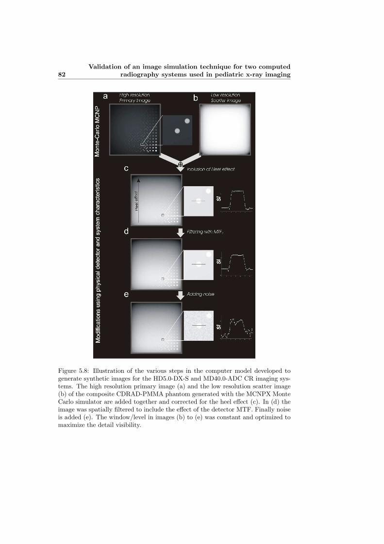
82Validation of an image simulation technique for two computed
radiography systems used in pediatric x-ray imaging
Figure 5.8: Illustration of the various steps in the computer model developed togenerate synthetic images for the HD5.0-DX-S and MD40.0-ADC CR imaging sys-tems. The high resolution primary image (a) and the low resolution scatter image(b) of the composite CDRAD-PMMA phantom generated with the MCNPX MonteCarlo simulator are added together and corrected for the heel effect (c). In (d) theimage was spatially filtered to include the effect of the detector MTF. Finally noiseis added (e). The window/level in images (b) to (e) was constant and optimized tomaximize the detail visibility.
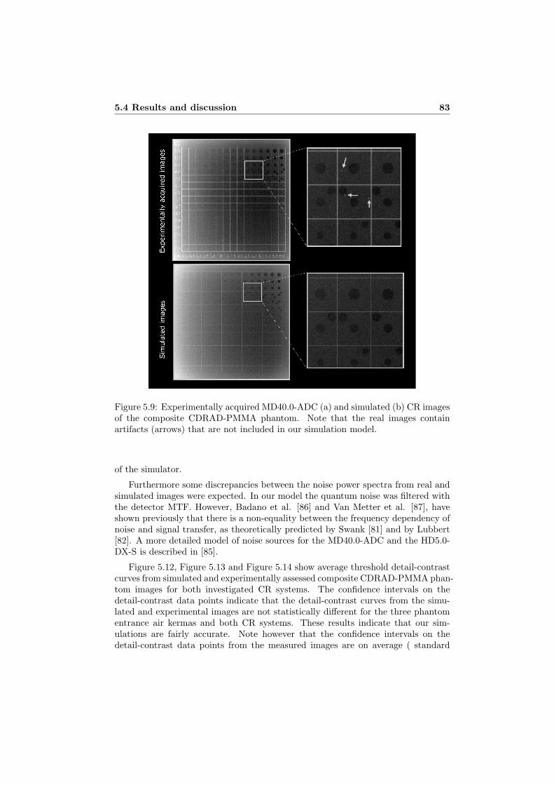
5.4 Results and discussion 83
Figure 5.9: Experimentally acquired MD40.0-ADC (a) and simulated (b) CR imagesof the composite CDRAD-PMMA phantom. Note that the real images containartifacts (arrows) that are not included in our simulation model.
of the simulator.
Furthermore some discrepancies between the noise power spectra from real andsimulated images were expected. In our model the quantum noise was filtered withthe detector MTF. However, Badano et al. [86] and Van Metter et al. [87], haveshown previously that there is a non-equality between the frequency dependency ofnoise and signal transfer, as theoretically predicted by Swank [81] and by Lubbert[82]. A more detailed model of noise sources for the MD40.0-ADC and the HD5.0-DX-S is described in [85].
Figure 5.12, Figure 5.13 and Figure 5.14 show average threshold detail-contrastcurves from simulated and experimentally assessed composite CDRAD-PMMA phan-tom images for both investigated CR systems. The confidence intervals on thedetail-contrast data points indicate that the detail-contrast curves from the simu-lated and experimental images are not statistically different for the three phantomentrance air kermas and both CR systems. These results indicate that our sim-ulations are fairly accurate. Note however that the confidence intervals on thedetail-contrast data points from the measured images are on average ( standard

84Validation of an image simulation technique for two computed
radiography systems used in pediatric x-ray imaging
0,00E+002,00E-064,00E-066,00E-068,00E-061,00E-051,20E-051,40E-051,60E-051,80E-052,00E-05
0,5 1 1,5 2 2,5 3Frequency (lp/mm)
NN
PS
Agfa ADC Compact (Subscan Direction)Agfa ADC Compact (Scan Direction)Agfa ADC Compact (Radial Direction)Agfa ADC Compact (Simulated)
Figure 5.10: NNPS for the MD40.0-ADC CR system. The NNPS were calculatedin experimentally acquired and simulated images of a 50 mm thick homogenousPMMA plate acquired at 65 kV and using a phantom entrance air kerma of 55µGy.
deviation) 37(32%) and 41(44%) larger than the confidence intervals on the detail-contrast data points from the simulated images for respectively the HD5.0-DX-Sand the MD40.O-ADC. This can be attributed to the fact that the real imagescontain image artifacts (e.g. Figure 5.9) that were not simulated. The HD5.0-DX-Sperforms overall very similarly for 55 and 110 µGy phantom entrance air kermas.For the three smallest hole depths and medium size hole depths of 0.8 mm and1mm, the performance is lower for a 22 µGy than for 55 µGy and 110 µGy phan-tom entrance air kermas. The MD40.0-ADC system performs overall very similarlyfor 22 µGy, 55 µGy and 110 µGy phantom entrance air kermas; the performancefor the 22 µGy phantom entrance air kerma is only lower for 0.5, 0.8 and for 5 mmhole depths.
At the same phantom entrance air kerma, the HD5.0-DX-S were significantly su-perior to the MD40.0-ADC system for all hole depths. These results are consistentwith the physical characteristics; for all phantom entrance air kerma the noise powerspectra of the HD5.0-DX-S (Figure 5.10) are lower than the noise power spectra ofthe MD40.0-ADC (Figure 5.11), while the detector MTF of the HD5.0-DX-S is su-perior to the detector MTF of the MD40.0-ADC (Figure 5.4). Moreover, clinicalstudies have shown that images acquired wit the HD5.0-DX-S were significant su-perior compared to images acquired with the MD40.0-ADC. Using the HD5.0-DX-Sa dose reduction of 75% can be achieved.
The superior image quality of the HD5.0-DX-S is mainly due to the difference

5.5 Conclusion 85
0,00E+00
1,00E-06
2,00E-06
3,00E-06
4,00E-06
5,00E-06
6,00E-06
0,5 1,5 2,5 3,5 4,5Frequency (lp/mm)
NN
PS
Agfa DX-S (CCD Direction)Agfa DX-S (Scan Direction)Agfa DX-S (Radial Direction)Agfa DX-S (Simulated)
Figure 5.11: NNPS for the HD5.0-DX-S CR system. The NNPS were calculatedin experimentally acquired and simulated images of a 50 mm thick homogenousPMMA plate acquired at 65 kV and using a phantom entrance air kerma of 55µGy.
in the structure of the phosphor. The needle structure phosphor of the HD5.0can channel light and thus reduce the spread of the laser light and the photo-stimulated light. Conversely, the standard powder phosphor used with the AgfaADC Compact has no structure and so the laser light diffuses more rapidly withdepth of penetration than with the structured phosphor [85]. Moreover, since thephosphor thickness of the HD5.0 is twice the thickness of the MD40.0, the quantumefficiency is about 60% higher for the HD5.0-DX-S [85].
5.5 Conclusion
A computer model, based on Monte Carlo techniques and physical characteristicsof the detector and imaging system, is developed and validated to simulate two CRimaging systems. This model can be used to maximize image quality and minimizedose in the CR images by optimizing the acquisition and processing parameters.Our model can also be used as a starting point to evaluate a variety of potentiallymore effective x-ray spectra, system geometries, image detectors etc. By givingmore complex anthropomorphic voxel phantom models as input, various image pro-cessing techniques can be evaluated. By using a variety on anthropomorphic voxelphantoms, typical limitations encountered in observer studies with physical anthro-pomorphic phantoms and patients, such as the lack of a variety of phantoms andabsence of knowledge of the ground truth respectively, can be overcome.

86Validation of an image simulation technique for two computed
radiography systems used in pediatric x-ray imaging
0,1
1
10
0,1 1 10
Contrast Depth (mm)
Co
ntr
ast
Dia
met
er (
mm
)
HD5.0-DX-S (exp)HD5.0-DX-S (sim)MD40.0-ADC (exp)MD40.0-ADC (sim)
Figure 5.12: Detail-contrast curves from simulated and experimentally assessedimages of the composite CDRAD phantom. The error bars indicate standard errorsin the average threshold diameter. The CD curves are shown for the phantomentrance air kermas: 22 µGy
0,1
1
10
0,1 1 10
Contrast Depth (mm)
Co
ntr
ast
Dia
met
er (
mm
)
HD5.0-DX-S (exp)HD5.0-DX-S(sim)MD40.0-ADC (exp)MD40.0-ADC (sim)
Figure 5.13: Detail-contrast curves from simulated and experimentally assessedimages of the composite CDRAD phantom. The error bars indicate standard errorsin the average threshold diameter. The CD curves are shown for the phantomentrance air kerma: 55 µGy

5.5 Conclusion 87
0,1
1
10
0,1 1 10
Contrast Depth (mm)
Co
ntr
ast
Dia
met
er (
mm
)
HD5.0-DX-S (exp)HD5.0-DX-S (sim)MD40.0-ADC (exp)MD40.0-ADC (sim)
Figure 5.14: Detail-contrast curves from simulated and experimentally assessedimages of the composite CDRAD phantom. The error bars indicate standard errorsin the average threshold diameter. The CD curves are shown for the phantomentrance air kerma: 110 µGy

Chapter 6
Cu filtration for dosereduction in neonatal chestimaging
• Smans K, Struelens L, Smet M, Vanhavere F, Bosmans H,“Cu filtrationfor dose reduction in neonatal chest imaging.” submitted for publication inRadiation Protection and Dosimetry at 30/06/09.
6.1 Abstract
As neonatal chest images are frequently acquired to investigate the life threateninglung diseases in prematurely born children, their optimisation in terms of X-rayexposure is required. The aim of this study was to investigate whether such doseoptimisation studies could be performed using a Monte Carlo computer model.More specific, we used a Monte Carlo computer model to investigate the influenceof Cu filtration on image quality and dose in neonatal chest imaging. Monte Carlosimulations were performed with the MCNPX code and used with voxel modelsrepresenting prematurely born babies (590 g and 1910 g). Physical image qualitywas derived from simulated images in terms of the signal difference-to-noise ratio(SDNR) and signal-to-noise ratio (SNR). To verify the simulation results we alsoperformed measurements using the Gammex 610 Neonatal Chest Phantom whichrepresents a 1-2 kg neonate. A figure of merit (FOM) was used to assist in evaluatingthe optimum balance between the image quality and the patient dose. Our resultsshow that our Monte Carlo computer model to investigate dose and image qualityworks well and can be used in dose optimisation studies for real clinical practices.Furthermore, working at a specific constant incident air kerma (Ka,I), additionalfiltration proved to increase SNR with 30% whereas working at a specific constantdetector dose, extra Cu filtration reduces the lung dose with 25%. Optimum balance
88

6.2 Introduction 89
between patient dose and image quality is found to be at 60 kVp (using extrafiltration).
6.2 Introduction
Lung disease represents one of the most life-threatening conditions in prematurelyborn children. Several of these infants may have lungs that are physiologically andmorphologically immature. This may lead directly to respiratory distress syndrome(RDS). The term respiratory distress syndrome (RDS) has come to represent theclinical expression of surfactant deficiency and its non-specific histologic counter-part, hyaline membrane disease. Another common disease is the bronchopulmonarydysplasia (BPD), alternatively termed chronic lung disease of infancy, a disorder oflung injury and repair. As RDS shows a granular lung pattern on the chest radio-graph, noise is very distracting and can interrupt the correct diagnosis.
The risks associated with x-ray examinations are low compared to the othermedical risks that these patients face, but even then, the radiation dose shouldbe kept as low as reasonable achievable. Previous studies showed that extra Cu-filtration lowers the radiation dose [88, 89, 90]. This way of obtaining dose reductionin pediatric radiology is also recommended by EC experts [25].
As computer processing capacity has been increased, dose calculations and imagesimulation using Monte Carlo techniques can nowadays be obtained in reasonablecomputational times. As a result Monte Carlo techniques allow the user to optimizea variety of aspects in the imaging chain such as x-ray spectra, system geometriesand acquisition parameters.
In present paper, we used a Monte Carlo computer model to study the influenceof Cu filtration for dose reduction in neonatal chest imaging. This was considereda first step towards more future applications.
6.3 Material and methods
6.3.1 Monte Carlo simulations
A Monte Carlo model was used to assess patient dose and image quality. The maincomponents of the imaging system were included in the simulation model, i.e., thex-ray spectrum, patient and image detector. All Monte Carlo calculations wereperformed using the Monte Carlo software package MCNPX version 2.5.0 [10]. Asmodel for the patient we used two voxel phantoms [91] representing prematurelyborn babies: voxel Phantom 1 (1910 g - 50 cm) and voxel Phantom 2 (590 g - 30cm). The image system modelled was the HD 5.0 CR plate (Agfa-HealthCare N.V.,Mortsel, Belgium) that is read out with the DX-S reader (Agfa-HealthCare N.V.,Mortsel, Belgium) as this is being used in our pediatric radiology department.
Clinically relevant radiation fields were placed to simulate chest radiographs(AP projection). The field size was 9.6 cm x 8 cm for Phantom 1 and 7 cm x 5 cm

90 Cu filtration for dose reduction in neonatal chest imaging
for Phantom 2; the source-skin distance (SSD) was 105 cm. In the simulations weused a source with a tube voltage ranging from 40 - 120 kVp and total filtrationequivalent to 3.8 mm of aluminum. To investigate the influence of extra filtrationwe used the same spectra (40 - 120 kVp, 3.8 mm Al total filtration) but addedextra Cu filtration. In this study we used the combination of 0.2 mm Cu and 1 mmAl which was also used in a previously published dose reduction study [90]. Thex-ray spectra were generated with the IPEM spectrum generator software [43]. Toassess patient dose using the simulation model mean lung doses were computed foreach combination of phantoms (Phantom 1 and Phantom 2) and for different beamqualities (40 - 120 kVp, with and without the additional 0.2 mm Cu + 1 mm Alfiltration).
To simulate images we calculated the absorbed energy in the HD 5.0 CR plate.This detector was modeled as a 250 µm thick CsBr:Eu2+ phosphor plate with asurface density of 0.17 g.cm−2. The detector was defined as a 4200 x 3408 arrayof detectors with a 100 µm x 100 µm mesh resolution. In a following step thosesimulated images were further modified, using physical characteristics of the imagingsystem, to account for the signal intensity variations due to the heel effect along theanode-cathode axis, the spatial resolution characteristics of the CR detector andthe various sources of image noise [92].
Physical image quality of the resulting simulated images (Figure 6.1) was derivedin terms of the signal-to-noise ratio, SNR, and the signal difference-to-noise ratio,SDNR. SNR is defined as the ratio of the mean signal of the object of interest So
and the standard deviation of the noise σo, whereas SDNR is defined as the ratiobetween the mean signal difference of the object of interest So and the backgroundSb, and the standard deviation of the noise σb in the background:
SNR =So
σo(6.1)
SDNR =Sb − So
σb(6.2)
To calculate SNR we chose a region of interest (ROI) in the lung region (So).To calculate SDNR we used an additional ROI in the heart region (Sb) (see Fig-ure 6.1). The rationale behind this choice is that radiologists are, for the particularapplications in the newborn children, in need for an optimal SDNR in the softtissues.
In this study we performed simulations for a constant incident air kerma. In-cident air kerma is the kerma to air from an incident X-ray beam measured onthe central beam axis at the position of the patient and excludes backscatteredradiation.
An incident air kerma (Ka,I) of 20 µGy was chosen based on previous clinicalstudies [26]. However, in clinical practice it is common to work with an automaticexposure control (AEC) cell that keeps the detector dose constant. As RDS ischaracterized by a granular lung pattern on the chest radiograph, noise (related

6.3 Material and methods 91
Figure 6.1: Simulated chest radiographs with a ROI in lung region and one in theheart region. (a) Phantom 1 with field size of 9.6 cm x 8 cm; (b) Phantom 2 withfield size of 7 cm x 5 cm.
to detector dose) is very distracting and can interrupt the correct diagnosis. Thismakes that radiologists prefer to work with a constant noise level in the image.Therefore we also performed simulations for a constant detector dose in the ROIlocated in the lung. Calculations were performed for a detector dose of 7 µGy.
6.3.2 Phantom measurements
In order to validate our simulation, phantom measurements were performed withthe Gammex 610 Neonatal Chest Phantom (Gammex, Inc., Middleton, WI, USA).This phantom represents a 1-2 kg neonate in its transmission characteristics, his-togram, physical size and structure. In this experiment we used a mobile x-rayunit (Mobilett III type P135/30R (Siemens)) with a total filtration of 3.8 mm Al.Phantom images were acquired for several beam qualities (60 - 70 kVp, with andwithout the additional 0.2 mm Cu + 1 mm Al filtration). Tube load (mAs) wasadjusted in order to have a constant incident air kerma (Ka,I) of 20 µGy. Theincident air kerma was measured with the Multi-Purpose Detector (MPD) of thebarracuda dose meter (RTI Electronics AB, Sweden) in the entrance plane of thephantom.
SNR and SDNR were calculated according to equation 6.1 and equation 6.2,with S denoting the signal intensities measured in linearized raw images. The ROIsare shown on Figure 6.2.
In a separate experiment, the average signal intensity (S) in a region of interestof the lung of the Gammex phantom was compared with S in images of PMMAplates of various thicknesses acquired with the same acquisition parameters as thepatients. It was shown that the lung region of the Gammex phantom is equivalentto 60 mm PMMA for a 65 kVp W-target x-ray beam. The same experiment wasperformed in MCNPX for the two voxel phantoms. The lung regions of the twovoxel phantoms are equivalent to respectively 45 mm PMMA (Phantom 1) and30 mm PMMA (Phantom 2). The properties of the phantoms are summarized inTable 6.1.

92 Cu filtration for dose reduction in neonatal chest imaging
Figure 6.2: Radiograph of the Gammex 610 anthropomorphic phantom a ROI inlung region and one in the heart region
Phantom 1 Phantom 2 Gammex(Monte Carlo) (Monte Carlo) (Measurements)
Weight 1910 g 590 g 1000 -2000 gThickness (total) 65 mm 50 mm 54 mmThickness (PMMA equiv.) 45 mm 30 mm 60 mm
Table 6.1: Phantoms used for optimisation..
6.3.3 Figure of merit (FOM)
A figure of merit (FOM) was used to assist in evaluating optimum balance betweenthe image quality and the dose to the patient. FOM is defined as SDNR squaredper unit exposure or - more preferably - dose [93]. In this study FOM was computedby dividing SDNR2 by the lung dose:
FOM =SDNR2
LungDose(6.3)
The FOM was only calculated for the voxel phantoms since for the GAMMEXphantom no lung dose measurements were possible.

6.4 Results and discussion 93
6.4 Results and discussion
6.4.1 Patient dose
Figure 6.3 and Figure 6.4 show the lung dose as a function of the beam qualitycalculated for respectively a constant entrance air kerma (Ka,I = 20 µGy) and aconstant detector dose (detector dose = 7 µGy). When working at a constant airkerma, the lung dose is increasing with increasing beam hardening (increasing kVpand adding 0.2 mm Cu + 1 mm Al). More specific the lung dose is increasing 13%on average when the extra filtration is used. When working at a constant detectordose (Figure 6.4), the lung dose is decreasing with 25% on average when extrafiltration is used.
0
5
10
15
20
25
30 50 70 90 110 130kVp
Lung
Dos
e [µ
Gy]
Phantom 1Phantom 1 (+Cu)Phantom 2Phantom 2 (+Cu)
Figure 6.3: Lung dose as a function of the beam quality for a chest radiograph ob-tained with Monte Carlo simulations for 2 voxel phantoms (Phantom1 and Phantom2). Simulations were performed for a Ka,I of 20 µGy, a total filtration of 3.8 mmAl (no extra filter) and the same 3.8 mm Al increased with 0.2 mm Cu + 1 mm Al(denoted by + Cu).
6.4.2 Image quality: SNR and SDNR
Figure 6.5 demonstrates the influence of the beam quality on SNR measurementsfor an incident air kerma of 20 µGy. For all phantoms SNR is increasing withincreasing beam hardening and decreasing patient size. This is not unexpectedsince the fraction of photons traveling through the body phantom and reaching thedetector surface will be higher, yielding a higher detector dose. SNR is the highest

94 Cu filtration for dose reduction in neonatal chest imaging
0
5
10
15
20
25
30
20 40 60 80 100 120kVp
Lung
dos
e (µ
Gy)
Phantom 1Phantom 1 (+ Cu)Phantom 2Phantom 2 (+ Cu)
Figure 6.4: Lung dose as a function of the beam quality for a chest radiograph ob-tained with Monte Carlo simulation for 2 voxel phantoms (Phantom1 and Phantom2). Simulations were performed for a detector dose of 7 µGy, a total filtration of3.8 mm Al (no extra filter) and the same 3.8 mm Al increased with 0.2 mm Cu +1 mm Al (denoted by + Cu).
for Phantom 2 (thinnest phantom, 30 mm PMMA equivalent) and the lowest forthe Gammex phantom (thickest phantom; 60 mm PMMA equivalent). Figure 6.5also shows that when working with additional filtration SNR is increasing 30% onaverage.
Since, in a photostimulable phosphor the detector dose is directly linked tothe signal intensities and noise in the resulting image, SNR will be constant whenworking at constant detector dose (not shown).
Figure 6.6 shows SDNR as a function of the beam quality when working at aconstant entrance air kerma (Ka,I = 20 µGy). Adding Cu filtration and increasingkVp, will harden the beam and compromise the signal differences in the images.However, the loss in signal difference will be partly compensated by the gain inSNR (Figure 6.5). This makes the SDNR reaching a maximum at 60 kVp for thetwo voxel phantoms and at 65 kVp for the Gammex phantom when extra filtrationis used. Phantom measurements and simulations show the same trend, however dueto the differences in anatomical structures SDNR is different for the three phantoms.
Figure 6.7 shows SDNR as a function of the beam quality when working at aconstant detector dose. Since the noise level in the images is constant (= con-stant detector dose) and the signal difference is decreasing due to increasing beamhardening, SDNR measurements will also decrease.

6.4 Results and discussion 95
0
20
40
60
80
100
120
30 50 70 90 110 130kVp
SN
R
Phantom 1Phantom 1 (+Cu)Phantom 2Phantom 2 (+Cu)GammexGammex (+Cu)
Figure 6.5: SNR as a function of the beam quality for a chest radiograph obtainedwith Monte Carlo simulation for 2 voxel phantoms (Phantom1 and Phantom 2) andexperimentally acquired images of the Gammex Neonatal Chest phantom. Simula-tions and measurements were performed for a Ka,I of 20 µGy, a total filtration of3.8 mm Al (no extra filter) and the same 3.8 mm Al increased with 0.2 mm Cu +1 mm Al (denoted by + Cu). SNR measurements were performed in an ROI in thelung region.
6.4.3 Optimisation: figure of merit (FOM)
FOM as a function of the beam quality is shown in Figure 6.8 (when workingat a constant air kerma) and in Figure 6.9 (when working at a constant detectordose). Optimal beam quality is found where FOM reaches its maximum. For bothsituations, working at a constant entrance air kerma and working at a constantdetector dose, optimum beam quality is found at 60 kVp using extra Cu filtration.Figure 6.8 and Figure 6.9 also show that optimum kVp is decreasing when extraCu filtration is used.
Our results agree with previously published results by Moore et al [88] and bySeifert et al [89]. However, a study published by Hansson et al [94] showed a clinicalpreference for higher kVp settings (optimum at 90 kVp). Those different findingscan be explained by the fact that FOM does not depend highly on kVp (as can beseen in Figure 6.8 and Figure 6.9).

96 Cu filtration for dose reduction in neonatal chest imaging
0
5
10
15
20
25
30
35
30 50 70 90 110 130kVp
SD
NR
Phantom 1Phantom 1 (+Cu)Phantom 2Phantom 2 (+Cu)GammexGammex (+Cu)
Figure 6.6: SDNR as a function of the beam quality for a chest radiograph obtainedwith Monte Carlo simulation for 2 voxel phantoms (Phantom1 and Phantom 2) andexperimentally acquired images of the Gammex Neonatal Chest phantom. Simula-tions and measurements were performed for a Ka,I of 20 µGy, a total filtration of3.8 mm Al (no extra filter) and the same 3.8 mm Al increased with 0.2 mm Cu + 1mm Al (denoted by + Cu). Signal difference was calculated for an ROI in the lungand in the heart.
6.5 Conclusion
This study showed that simulations and phantom measurements have the sametrend. Moreover, the results showed that optimisation between dose and imagequality can be obtained by altering the beam quality, more specifically by addingextra Cu filtration. Those results agree with previously published papers investigat-ing neonatal chest imaging [88, 89]. This confirms that our Monte Carlo computermodel to investigate dose and image quality works well and consequently can beused in dose optimisation studies for real clinical practices.
Furthermore optimum balance between patient dose and image quality is foundto be at 60 kVp using additional filtration. When working at a constant incident airkerma, additional filtration proved to increase SNR with 30%. On the other hand,working at a constant detector dose the lung dose will decrease 25% on average usingextra Cu filtration. Extra Cu filtration can be installed on all systems, however,if the tube output of the systems is not high enough, exposure time will be longand will introduce motion artifacts. In our hospital, this study will be followed bya clinical trial.

6.5 Conclusion 97
0
5
10
15
20
25
30
35
20 40 60 80 100 120kVp
SD
NR
Phantom 1Phantom 1 (+Cu)Phantom 2Phantom 2 (+Cu)
Figure 6.7: SDNR as a function of the beam quality for a chest radiograph obtainedwith Monte Carlo simulation for 2 voxel phantoms (Phantom1 and Phantom 2).Simulations were performed for a detector dose of 7 µGy, a total filtration of 3.8mm Al (no extra filter) and the same 3.8 mm Al increased with 0.2 mm Cu + 1mm Al (denoted by + Cu). Signal difference was calculated for an ROI in the lungand in the heart.

98 Cu filtration for dose reduction in neonatal chest imaging
0
5
10
15
20
25
30
35
40
45
50
30 50 70 90 110 130kVp
FO
M
Phantom 1
Phantom 1 (+Cu)
Phantom 2
Phantom 2 (+Cu)
Figure 6.8: FOM as a function of the beam quality for a chest radiograph obtainedwith Monte Carlo simulation for 2 voxel phantoms (Phantom1 and Phantom 2).Simulations were performed for a Ka,I of 20 µGy, a total filtration of 3.8 mm Al(no extra filter) and the same 3.8 mm Al increased with 0.2 mm Cu + 1 mm Al(denoted by + Cu).

6.5 Conclusion 99
0
5
10
15
20
25
30
35
40
45
50
0 20 40 60 80 100 120 140kVp
FO
M
Phantom 1Phantom 1 (+ Cu)Phantom 2Phantom 2 (+ Cu)
Figure 6.9: FOM as a function of the beam quality for a chest radiograph obtainedwith Monte Carlo simulation for 2 voxel phantoms (Phantom1 and Phantom 2).Simulations were performed for a detector dose of 7 µGy, a total filtration of 3.8mm Al (no extra filter) and the same 3.8 mm Al increased with 0.2 mm Cu + 1mm Al (denoted by + Cu).

Summary
General radiation protection principles require that radiation doses of the patientsshould be as low as reasonably achievable (ALARA-principle) with the medical pur-poses. In Europe the directive 97/43/Euratom requires that special attention shouldbe given to the patient dose in pediatric examinations, of which premature babiesconstitute an important sub-group. Risks associated with x-ray examinations arelow compared to the other medical risks that these patients face, but even then, theradiation dose should be kept as low as reasonably achievable. The radiation doseis however linked to image quality and the image quality may not be lowered so farthat it endangers the diagnostic or therapeutic outcome of a radiographic proce-dure. Therefore radiation dose and image quality should be balanced. In Belgiumno information about dose and image quality of radiographs in neonates was avail-able. Furthermore, due to the recent shift from conventional film-screen imagingtowards computed radiography (CR), the medical team in pediatric radiology andthe head of our department were wondering if exposure settings that had been setfor film-screen system were also appropriate for computed radiography. Moreoverthey were interested in the effect of additional filtration. Trying to answer thosequestions in a scientifically way prompted us to start this study.
Radiation dose
Knowledge of the radiation dose was a first step in the optimisation process. Astudy on 255 premature children in our hospital found that they undergo 10 x-ray examinations, on the average. In this sample, the maximum was 78 x-rayexaminations. To assess the patient dose we performed 60 measurements of theentrance surface dose (ESD) for a chest radiograph. In this group, the averagepatient weight was 1.9 kg and the median ESD was 34 µGy (3-101 µGy). This isbelow the European reference dose of 80 µGy for neonates of 1.0 kg and well belowthe European reference dose of 135 µGy for babies 10 months old.
Moreover, 12 dose area product (DAP) measurements were acquired. The me-dian DAP-value was 7.1 mGy.cm2 (3.5 - 32.4 mGy.cm2) which is also comparablewith data from the literature. However, there was a large spread in this limiteddata set. Further investigation showed that this was due to inappropriate collima-tion of the radiation field. A field which is too large will not only impair the image
100

Summary 101
contrast and resolution by increasing the amount of scattered radiation but also -most importantly - result in unnecessary irradiation of the patient. Correct beamlimitation requires proper knowledge of the external anatomical landmarks by thetechnician. This illustrates the need for both theoretical and practical teaching ofthe technicians.
To convert those measured dose values into doses in specific organs and in theentire body, we developed voxel phantoms representing prematurely born babies.Based on CT- and MRI-images two voxel phantoms were created: Phantom 1 (1910g) and Phantom 2 (590 g). Using those phantoms, conversion coefficients betweenESD/DAP and organ doses were calculated with the Monte Carlo software pack-age MCNPX. The results were compared with the commercially available softwarepackage PCXMC in which the available mathematical phantoms can be downsizedtowards the prematurely born baby.
For organs within the radiation field the conversion coefficients calculated withthe voxel phantoms correlated well with those calculated with the PCXMC pro-gram. Therefore, the simple phantom-scaling method used in PCXMC seemedto be sufficient for these purposes. However, one should note that there will beconsiderable uncertainty on doses to organs that are partly or totally outside theradiation field, because the actual primary beam location in the patient and patientanatomy cannot be exactly reproduced in simulations. As expected differences inskeletal structure and RBM/bone distributions between the phantom models devel-oped here and those specified in PCXMC give rise to variations in bone and RBMdose conversion factors.
In our hospital the lung dose in a 2 kg prematurely born baby (with ESD 34µGy) who is exposed to an average of 10 chest radiographs is of the order of 250µGy. If 80 radiographs are required, the dose to the lung will be approximately 2.0mGy. Compared to the other medical risks that these patients face, the radiationrisks associated with these x-ray examinations are low. However, we do not know ifthe radiation exposures are as low as reasonably achievable. In order to investigateif patient dose can be lowered, we also needed to assess image quality. Assessmentof image quality was based on simulated images.
Image quality
Image simulation was performed in two steps. In a first step a Monte Carlo techniquewas used to yield realistic modelling of primary and scattered radiation incident onan x-ray detector. In MCNPX, image generation can be performed using a prede-fined detector model, the radiography tally, which accordingly to the manual, canbe used to generate radiographic images. This radiography tally has been used pre-viously in image simulation studies. However, validation, based on the calculationof scatter to primary ratio’s (SPRs), showed that this detector model was inappro-priate and overestimated the scattered radiation. We therefore developed two othermethods to simulate accurate images (pixel size 100 µm) with MCNPX. Simulationswere performed for a perfect energy integrating detector and for a photostimulable

102 Summary
phosphor plate used in computed radiography. Unlike the perfect energy integrat-ing detector model, the model for the photostimulable phosphor plate takes intoaccount the spectral sensitivity of the detector material. For this model an excel-lent agreement was found between calculated scatter-to-primary radios (SPRs) anddata published in literature, moreover, physical SPR measurements were comparedagainst Monte Carlo data with excellent agreement. Our approach is unique as itwas validated successfully for a range of parameters of interest, which included thex-ray field of view, x-ray energy, air gap, phantom thickness and detector composi-tion. Moreover, using our approach we can simulate images in acceptable computertimes.
In a next study, the simulated images were modified, using physical character-istics of the imaging system to account for the signal intensity variations due tothe heel effect along the anode-cathode axis, the spatial resolution characteristicsof the CR detectors and the various sources of image noise. To evaluate our com-puter model, a quantitative comparison was performed between synthetic imagesof a contrast-detail phantom generated with our computer model and experimen-tally acquired images of a physical version of this phantom. In this study we usedthe CDRAD contrast-detail phantom. Typical acquisition parameters for pediatricchest x-ray examinations were evaluated. Threshold-contrast curves were computedfor the synthetic and experimentally acquired images using a commercially avail-able scoring program. Good agreement was shown between the threshold-contrastcurves of synthetic and real images. This implies that our simulation model is ableto accurately simulate the real imaging systems.
Optimisation
In the last part the simulation model was used to investigate if using extra copperfiltration in the beam could reduce the lung dose without endangering image qual-ity in chest radiographs. Monte Carlo simulations coupled with the voxel modelsrepresenting prematurely born babies (590 g and 1910 g) were performed to in-vestigate dose and image quality. Image quality was derived from simulated chestradiographs in terms of signal-difference-to-noise ratio (SDNR) and signal-to-noiseratio (SNR) of anatomical structures corresponding to the image criteria.
When working at a constant incident air kerma, additional filtration provedto increase SNR with 30%. On the other hand, working at a constant detectordose, incident air kerma will decrease 30% and lung dose will decrease 25% usingadditional Cu filtration.
A figure of merit (FOM) was used to assist in evaluating which tube potentialachieved optimum balance between the image quality and the dose to the patient.The FOM was computed by dividing SDNR2 by the lung dose. For the CR systemused in our hospital optimum balance between patient dose and image quality wasfound at 60 kVp using additional Cu filtration. When no filtration is used optimumkVp is found at 80 kVp, which is higher than the film-screen exposure parameterscurrently used (60 kVp - 70 kVp without extra Cu filtration).

Summary 103
Practical aspects
Since the film-screen exposure parameters are not appropriate for CR imaging,exposure parameters (kVp and filtration) should be changed:
• If it is possible extra Cu filtration (0.2 mm Cu + 1 mm Al) should be used.Using extra Cu filtration, peak tubevoltage should be 60 kVp.
• If it is not possible to use extra Cu filtration, the peak tubevoltage should beincreased to 80 kVp.
Moreover, as RDS is characterized by a granular lung pattern on the chestradiograph, noise (related to detector dose) is very distracting and can interruptthe correct diagnosis. Therefore radiologists prefer to work with a constant noiselevel in the image. This can be obtained by keeping the detector dose constant. Inorder to do so mAs values need to be adjusted based on the patient weight.
Note that extra Cu filtration can only be installed on systems if the tube outputis high enough. If not, exposure time will be excessively long and will introducemotion artifacts. Fortunately in our hospital the tube output is sufficiently high. Aclinical trial using 60 kVp, 0.2 mm Cu + 1 mm Al and adjusted mAs settings willbe started shortly.
Future outlook
In this study we used the simulation model to find a balance between dose and imagequality in neonatal chest imaging, however, the image simulation model as proposedin present work could be used for many more applications. The current approach,using Monte Carlo techniques in combination with physical characteristics of theimaging system, gives insight in the image formation process. It allows the userto evaluate and optimize a variety of aspects in the imaging chain such as x-rayspectra, system geometries, acquisition parameters and radiation dose (Figure 6.10).This makes the image simulation model a valuable tool in the evaluation and thedesign of new detectors, characterized by their spatial resolution, noise and detectorefficiency.
The image simulation model can also be used to generate highly realistic syn-thetic images of many variations of (complex) ground truth phantoms from a specificimaging system. This offers new perspectives for which many more applicationscould be worked out. The computer model gives the analyst the ability to per-form experiments not possible in the lab. Using realistic patient phantoms, a hugeamount of experiments can be done without patient irradiation. This is importantin the frame of increasing awareness for ethics. Moreover, simulated images can beuseful in the design and evaluation of image quality test objects.

104 Summary
Figure 6.10: Monte Carlo based simulation model to evaluate and optimize a varietyof aspects in the imaging chain such as x-ray spectra, system geometries, acquisitionparameters and radiation dose.
Nowadays, due to ongoing research and technological development, radiology isstill an evolving medical specialty. More than one century after the discovery ofx-rays in 1895, this study showed, that there is still room for optimisation of patientdose and image quality. We noticed that new detector technologies give rise toquestions about patient dose and image quality. In order to find a balance betweendose and image quality it is important to understand the basic physics involved inthe image formation process. We hope that the simulation model developed in thisstudy will be a valuable tool in the future.

Bibliography
[1] H.E. Johns; J.R. Cunningham. Physics of Radiology. Illinois, 1983.
[2] J.T. Bushberg; J.A. Seibert; E.M. Leidholdt and J.M. Boone. The EssentialPhysics of Medical Imaging. Lippincott Williams and Wilkins, Philadelphia,PA, 2001.
[3] International Commission on Radiological Protection. Recommendations ofthe International Commission on Radiological Protection, IRCP Publication60. Oxford, 1991.
[4] International Commission on Radiological Protection. Recommendations of theInternational Commission on Radiological Protection, IRCP Publication 103.Oxford, 2007.
[5] A. Wambersie; J. Zoetelief; H.G. Menzel; H. Paretzke. The icru: its contribu-tion to dosimetry in diagnostic and interventional radiology. Rad. Prot. Dos.,117:7–12, 2006.
[6] United Nations Scientific Committee on the Effects of Atomic Radiation.Sources and effect of ionizing radiation, Annex D. UNSCEAR, New York,2000.
[7] E. Vano; L. Gonzalez; J.M. Fernandez and E. Guibelalde. Patient dose valuesin interventional radiology. Br. J. Radiol., 86(815):1215–1220, 1995.
[8] G. Drexler; W. Panzer; L. Widenmann; G. Williams and M. Zankl. The calcu-lation of dose from external photon exposures using reference human phantomsand monte-carlo methods, part iii. Technical Report GSF 11/90, National Cen-ter for Environment and Health, Neuherberg, 1990.
[9] D. Hart; D.G. Jones and B.R. Wall. Estimation of effective dose in diagnosticradiology from entrance surface dose and dose-area product measurements.Technical Report NRPB-R262, NRPB, Chilton, 1994.
[10] L. Waters. MCNPX Users Manual. Los Alamos National Laboratory, LosAlamos, NM, 2002.
105

106 BIBLIOGRAPHY
[11] J.M. Boone. Handbook of Medical Imaging, volume 1. SPIE, Bellingham, WA,2000.
[12] International Electrotechnical Commission. Medical electrical equipment-characteristics of digital imaging devices: Determination of quantum efficiency,volume IEC 62220-1. IEC, Geneva, 2003.
[13] M.A.O. Thijssen; K.R. Bijkerk and R.J.M. van der Burght. Manual Contrast-Detail Phantom ARTINIS CDRAD type 2.0. Artinis Medical Systems bv,Andelst, The Netherlands.
[14] Artinis Medical Systems bv, Andelst, The Netherlands. Artinis CDRAD Anal-yser Version 1.1.
[15] A. Pascoal; C.P. Lawinski; I. Honey and P. Blake. Evaluation of a softwarepackage for automated quality assessment of contrast-detail images - compari-son with subjective visual assessment. Phys. Med. Biol., 50:5743–5757, 2005.
[16] Committee on the Biological Effects of Ionizing Radiations (BEIR V). Healtheffects of exposure to low levels of ionizing radiation. National Academy Press,Washington, DC, 1990.
[17] Commission for the European Communities. Council Directive 97/43 Eura-torm on health protection of individuals against dangers of ionizing radiationin relation to medical exposures, volume L180. Off. J. Eur. Commun., 1997.
[18] J.F. Chateil. Practical measurement of radiation dose in paediatric radiology.Radiology, 85:619–625, 2004.
[19] C. I. Armpilia; I. A. J. Five and P. L. Croasdale. Radiation dose quantitiesand risk in neonates in a special care baby unit. Br. J. Radiology, 75:590–595,2002.
[20] N. F. Jones; T. W. Palarm and I. S. Negus. Neonatal chest and abdominalradiation dosimetry: a comparison of two radiographic techniques. Br. J.Radiology, 75:920–925, 2001.
[21] R. Mooney and P. S. Thomas. Dose reduction in a paediatric x-ray departmentfollowing optimization of radiographic technique. Br. J. Radiology, 71:852–860,1998.
[22] B. J. McParland; W. Gorka and R. Lee. Radiology in the neonatal intensivecare unit: dose reduction and image quality. Br. J. Radiology, 69:929–937,1996.
[23] C. M. Wraith; C. J. Martin and E. J. N. Stockdale. An investigation intotechniques for reducing doses from neonatal radiographic examinations. Br. J.Radiology, 68:1047–1082, 1995.
[24] C. J. Martin; B. Farquhar; E. Stockdale and S. MacDonald. A study of the rela-tionship between patient dose and size in paediatric radiology. GastrointestinalEndoscopy, 67:864–871, 1994.

BIBLIOGRAPHY 107
[25] European Commission. European Guidelines on Quality Criteria for DiagnosticRadiographic Images in Paediatrics, volume EUR 16261. European Commis-sion, 1996.
[26] K. Smans; E.Vano; R. Sanchez; F.W.Schultz; J. Zoetelief and et al. Results ofa european survey on patient doses in paediatric radiology. Rad. Prot. Dos.,2008.
[27] M. Cristy and K.F. Eckerman. Specific absorbed fractions of energy of variousages from internal photon sources. Technical Report ORNL/TM-8381, OakRidge National Laboratory, Oak Ridge National Laboratory, Oak Ridge, TN,USA, 1987.
[28] M. Cristy. Mathematical phantoms representing children of various ages forus in estimates of internal dose. Technical Report ORNL/TM-367, Oak RidgeNational Laboratory, Oak Ridge National Laboratory, Oak Ridge, TN, USA,1980.
[29] H.L. Fisher; W.S. Snyder. Distribution of dose in the body from a source ofgamma rays distributed uniformly in an organ. Technical Report ORNL-4168,Oak Ridge National Laboratory, Oak Ridge National Laboratory, Oak Ridge,TN, USA, 1967.
[30] M. Tapiovaara; M. Lakkisto and A. Servomaa. Pcxmc. a pc based monte carloprogram for calculating patient dose in medical x-ray examinations. Techni-cal Report Report No. STUK-A139, Finish Center for Radiation and NuclearSafety. Finland, 1997.
[31] I.G. Zubal; C.R. Harrell; E.O. Smith; Z. Rattner; G. Gindi and P.B. Hof-fer. Computerized three-dimensional segmented human anatomy. Med. Phys.,21:299–302, 1994.
[32] M. Zankl; R. Veit; G. Williams; K. Schneider; H. Fendel; N. Petoussi andG. Drexler. The construction of computer tomographic phantoms and theirapplication in radiology and radiation protection. Radiat. Environ. Biophys.,27:153–164, 1988.
[33] N. Petoussi-Hens; M. Zankl; U. Fill and A. Regulla. The gsf family of voxelphantoms. Phys. Med. Biol., 47:89–106, 2002.
[34] J.C. Nipper; J.L. Williams and W.E. Bolch. Creation of two tomographicvoxel models of pediatric patients in the first year of life. Phys. Med. Biol.,47:3143–3164, 2002.
[35] C. Lee; J.L. Williams; C. Lee and W.E. Bolch. The uf series of tomographiccomputational phantoms of pediatric patients. Med. Phys., 32:3537–48, 2005.
[36] C. Lee; C. Lee; J.L. Williams and W.E. Bolch. Whole-body voxel phantoms ofpaediatric patients-uf series b. Phys. Med. Biol., 51:4649–61, 2006.

108 BIBLIOGRAPHY
[37] C. Lee; D. Lodwick; J. Hasenauer; J.L. Williams; C. Lee and W.E. Bolch. Hy-brid computational phantoms of the male and female newborn patient: Nurbs-based whole body models. Phys. Med. Biol., 52:3309–3333, 2007.
[38] M. Caon; G. Bibbo and J. Pattison. An egs4-ready tomographic computa-tional model of a 14-year-old female torso for calculating organ doses from ctexaminations. Phys. Med. Biol., 44:2213–225, 1999.
[39] A. Fanaroff; B. Stoll; L. Wright; W. Carlo and R. Ehrenkranz. Trends inneonatal morbidity and mortality for very low birthweight infants. Am. J.Obstet. Gynecol., 196:147.e1 – 147.e8, 2007.
[40] D. Loeckx. Automated nonrigid intra-patient image registration using B-splines. PhD thesis, K.U.Leuven, Leuven, Belgium, 2006.
[41] International Commission on Radiological Protection. Basic Anatomical andPhysiological Data for Use in Radiological Protection: Reference Values, ICRPPublication 89. Oxford, 2002.
[42] K.A. Van Riper. Scan2MCNP software for Windows, version 1.06. WhiteRock Science, Los Alamos, USA.
[43] IPEM, York, UK. Catalogue of Diagnostic x-ray Spectra and other Data,IPEM-78.
[44] International Commission on Radiation Units and Measurements. Photon,Electron and Neutron Interaction Data for Body Tissues, Report 46. IPEM,Bethesda, MD, 1992.
[45] R. Kramer; J.W. Vieira; H.J. Khoury; F.R.A. Lima and D. Fuelle. All aboutmax: a male adult voxel phantom for monte carlo calculations in radiationprotection dosimetry. Phys. Med. Biol., 48:1239–1262, 2003.
[46] S.D. King and F.W. Spiers. Photoelectron enhancement of the absorbed dosefrom x-rays to human bone marrow: experimental and theoretical studies. Br.J. Radiol., 58:345–356, 1985.
[47] International Commission on Radiological Protection. Basic Anatomical andPhysiological Data for use in Radiological Protection: The Skeleton, ICRPPublication 70. Oxford, 1995.
[48] M. Cristy. Active bone marrow distribution as a function of age in humans.Phys. Med. Biol., 26:389–400, 1981.
[49] G.D. Kerr and K.F. Eckerman. Neutron and photon fluence-to-dose conversionfactors for active marrow of the skeleton. Proceedings of the fifth symposium onneutron dosimetry, Vol I, Radiation protection aspects(EUR 9762 EN), 1985.CEC, Luxembourg.
[50] J.M. Bland; D.G. Altman. Statistical method for assessing agreement betweentwo methods of clinical measurement. The Lancet, pages 307–310, 1986.

BIBLIOGRAPHY 109
[51] F. Rypens; T. Metens; N. Rocourt and P. Sonigo. Fetal lung volume: estimationat mr imaging: initial results. Radiology, 219:236–241, 2001.
[52] D.G. Jones and W.F. Wall. Organ doses from medical x-ray examinations cal-culated using monte carlo techniques. Technical Report NRPB-R186, NRPB,HMSO, London, UK, 1985.
[53] D. Hart; D.G. Jones and B.F. Wall. Normalised organ doses for paediatricx-ray examinations calculated using monte carlo techniques. Technical ReportNRPB-SR279, NRPB, Chilton, UK, 1996.
[54] J. Wilpshaar; E.C. Jokes; F.T.H. Lim; G.A.M. Van Leeuwen; P.J.Van denBoogaard; H.H.H. Kanhai; R. Willemze and J.H.F. Falkenburg. Magneticresonance imaging of fetal bone marrow for quantitative definition of the humanfetal stem cell compartment. Blood, 100:451–457, 2002.
[55] G. Drexler; W. Panzer; N. Petoussi and M. Zankle. Effective dose-how effectivefor patients? Radiat. Environ. Biophys., 32:209–219, 1993.
[56] C.J. Martin. Effective dose: How should it be applied to medical exposures?Br. J. Radiol., 80:639–647, 2007.
[57] J.M. Boone and V.N. Cooper. Scatter/primary in mammography: Monte carlovalidation. Med. Phys., 27(8):1818–1831, 2000.
[58] I. Sechopoulos; S. Suryanarayanan; S. Vedentham; C.J. D’Orsi and A. Karellas.Scatter radiation in digital tomosynthesis of the breast. Med. Phys., 34(2):564–576, 2007.
[59] Z. Jing; W. Huda and J.K. Walker. Scattered radiation in scanning slot mam-mography. Med. Phys., 25(7):1111–1117, 1998.
[60] D.E. Peplow and K. Verghese. Digital mammography image simulation usingmonte carlo. Med. Phys., 27(3):568–579, 2000.
[61] I. Sechopoulos and C. Ghetti. Optimization of the acquisition geometry indigital tomosynthesis of the breast. Med. Phys., 36(4):1199–1207, 2009.
[62] I.S. Kyprianou; A. Badal; A. Badano; D. Bahn; M. Freed; K.J. Myers andL. Thompson. Monte carlo simulated coronary angiograms of realistic anatomyand pathology models), journal = Proc. SPIE, year = 2009, volume = 6509,.
[63] E.M. Souza; S.C.A. Correa; A.X. Silva; R.T. Lopes and D.F. Oliveira. Method-ology for digital radiography simulation using the monte carlo code mcnpx forindustrial applications. Appl. Radiat. Isot., 66(5):587–592, 2008.
[64] S.C.A. Correa; E.M. Souza; A.X. Silva; R.T. Lopes and H. Yoriyaz. Dose-image quality study in digital radiography using monte carlo simulation. Appl.Radiat. Isot., 66(9):1213–1217, 2008.

110 BIBLIOGRAPHY
[65] M. Ramos; S. Ferrer; J.I. Villaescusa; G. Verdu and J.M. Campayo. Montecarlo image reconstruction of a mammographic phantom. Proceedings of the26th Annual International Conference of the IEEE EMBS, San Francisco, CA,USA, 2004.
[66] W. R. Nelson; N. Hirayama and D.W.O. Rogers. The egs4 code system. Tech-nical Report SLAC-Report-265, Stanford Linear Accelerator Center, 1985.
[67] S. Agostinelli et al. Geant4 - a simulation toolkit. Nucl. Instrum. MethodsPhys., Res. A 506:250–303, 2003.
[68] A.-K. Carton; R. Acciavatti; J. Kuo and A.D.A. Maidment. The effect ofscatter and glare on image quality in contrast-enhanced breast imaging usingan a-si/csi(tl) full-field flat panel detector. Med. Phys., 36(3):920–928, 2009.
[69] E. Samei. Image quality in two phosphor-based flat panel digital radiographicdetectors. Med. Phys., 30(7):1747–1757, 2003.
[70] N.W. Marshall. A comparison between objective and subjective image qualitymeasurements for a full field digital mammography systems. Phys. Med. Biol.,51:2441–2463, 2006.
[71] S. Rivetti; N. Lanconelli; R. Campanini; M. Bertolini; G. Borasi; A. Nitrosi;C. Danielli; L. Angelini and S. Maggi. Comparison of different ffdm units bymeans of physical characterization and contrast-detail analysis. Med. Phys.,33:4198–4209, 2006.
[72] I.D. Honey; A. MacKenzie and D.S. Evans. Investigation of optimum energiesfor chest imaging using film-screen and computed radiography. Br. J. Rad.,78:422–427, 2005.
[73] G. Ullman; M. Sandborg; D.R. Dance; R.A. Hunt and G. Alm Carlsson. To-wards optimization in digital chest radiography using monte carlo modeling.Phys. Med. Biol., 51(11):2729–2743, 2006.
[74] C. Ghettie; A. Borrini; O. Ortenzia; R. Rossi and L. Ordnez. Physical char-acteristics of ge senography essential and ds digital mammography detectors.Med. Phys., 35:456 – 463, 2008.
[75] J.A. Rowlands. The physics of computed radiography. Phys. Med. Biol.,47:R123–R166, 2002.
[76] K. Smans; L. Struelens; M. Smet; H. Bosmans and F. Vanhavere. Patient dosein neonatal units. Rad. Prot. Dos., 131(1):143–147, 2008.
[77] The MathWorks Inc. Matlab Version 7.0, 2004.
[78] S. Sarkar M. Adib M.R. Ay, M. Shahriari and H. Zaidi. Monte carlo simula-tion of x-ray spectra in diagnostic radiology and mammography using mcnp4c.Phys. Med. Biol., 49:4897–4917, 2004.

BIBLIOGRAPHY 111
[79] L. Struye A.D. Maidment Y.H. Kao M. Albert H. Bosmans A.K. Carton,D. Vandenbroucke and G. Marchal. Validation of mtf measurement for dig-ital mammography quality control. Med. Phys., 32(6):1684–95, 2005.
[80] D.S. Evans; A. Workman and M. Payne. A comparison of the imaging proper-ties of ccd-based devices used for small field digital mammography. Phys. Med.Biol., 47:117–135, 2002.
[81] R.K. Swank. Calculation of modulation transfer functions of x-ray fluorescentscreens. Appl. Opt., 12:1865–1870, 1973.
[82] G. Lubberts. Random noise produced by x-ray fluorescent screens. J. Opt.Soc. Am., 58:1475–83, 1968.
[83] N. Karssemeijer and M.A.O. Thijssen. Determination of contrast-detail curvesof mammography systems by automated image analysis. Proceedings of the 3rdInternational Workshop on Digital Mammography, pages 155–160, 1996.
[84] A.C. Davison; D. Hinkley. Bootstrap Methods and their Applications. Cam-bridge: Cambridge Series in Statistical and Probabilistic Mathematics, 2006.
[85] A. Mackanzie and I.D. Honey. Characterization of noise sources for two gener-ations of computed radiography systems using powder and crystalline photo-stimulable phosphors. Med. Phys., 34:3345–57, 2007.
[86] A. Badano; R.M. Gagne; B.D. Gallas; R.J. Jennings; J.S. Boswell and K.J.Myers. Lubberts effect in columnar phosphors. Med. Phys., 31:3122–3131,2004.
[87] R. Van Metter and M. Rabbani. An application of multivariate moment-generating functions to the analysis of signal and noise propagation in radio-graphic screen-film system. Med. Phys., 17:65–71, 1990.
[88] Moore C.S.; Beavis A.W. and Saunderson J.R. Investigation of optimum x-ray beam tube voltage and filtration for chest radiography with a computedradiography system. Br. J. Rad., 81:771–777, 2008.
[89] Seifert H.; Jesberger H.J.; Schneider G.; Rein L.; Blass G.; Limbach H.G.;Niewald M.; Sitzmann F.C. and Kramann B. Dose reduction in thorax radiog-raphy in simulated neonates with additional filtration and digital luminescenceradiography. Acta Radiol., 39(5):514–519, 1998.
[90] M.A. Staniszewska; T. Bieganski; A. Midel and D. Baranska. Filters for dosereduction in conventional x-ray examinations of children. Rad. Prot. Dos.,90:127–133, 2000.
[91] K. Smans; M. Tapiovaara; M. Cannie; L. Struelens; F. Vanhavere; M. Smet andH. Bosmans. Calculation of organ doses in x-ray examinations of prematurebabies. Med. Phys., 35(2):556–568, 2007.

112 BIBLIOGRAPHY
[92] K. Smans; H. Pauwels; F. Rogge; L. Struelens; O. Dragusin; F. Vanhavere andH. Bosmans. A simulation framework for pre-clinical studies on dose and imagequality: concepts and first validation. Proc. SPIE, 6913G, 2008.
[93] E. Samei; J.T. Dobbins; J.Y. Lo and M.P. Tornai. A framework for optimisingthe radiographic technique in digital x-ray imaging. Rad. Prot. Dos., 114:220–229, 2005.
[94] J. Hansson; M. Bath; M. Hakansson; H. Grundin; E. Bjurklint; P. Overstad;A. Kjellstrom; H. Bostrom; M. Jonsson; K. Jonsson and L.G. Mansson. An op-timisation strategy in a digital environment applied to neonatal chest imaging.Rad. Prot. Dose., 114(278-285), 2005.

List of publications
International journal
1. K. Smans, H. Bosmans, M. Xiao, A.K. Carton, G. Marchal, “Towards aproposition of a diagnostic (dose) reference level for mammographic acqui-sitions in breast screening measurements”, Radiat Prot Dosimetry, 117 (1-3):321–326, 2006
2. L. Struelens, L. Hambach, N. Buls, K. Smans, F. Malchair, M.T. Hoor-naerts, F. Vanhavere, B. Bosmans, “Image quality assessment using the CD-DISC phantom for vascular radiology and vascular surgery”, Eur J Radiol, 67(2):348–356, 2007
3. F. Bleeser, M.T. Hoornaert, K. Smans, L. Struelens, N. Buls, D. Berus, P.Clerinx, L. Hambach, H. Bosmans “Diagnostic reference levels in angiogra-phy and interventional radiology: a Belgian multi-center study”, Radiat ProtDosimetry, 129 (1-3):50–55, 2008
4. O. Dragusin, M. Gewillig, W. Desmet, K. Smans, L. Struelens, B. Bosmans,“Radiation dose survey in paediatric cardiac catherisation laboratory equippedwith flat-panel detectors”, Radiat Prot Dosimetry, 129 (1-3):91–95, 2008
5. K. Smans, E. Vano, R. Sanchez, F.W. Schultz , J. Zoetelief, T. Kiljunen, C.Maccia, H. Jarvinen, R. Bly, A. Kosunen, K. Faulkner, H. Bosmans “Resultsof a European survey on patient doses in paediatric radiology”, Radiat ProtDosimetry, 129 (1-3):204–210, 2008
6. K. Smans, L. Struelens, M.T. Hoornaert, F. Bleeser, N. Buls, D. Berus, P.Clerinx, F. Malchair, F. Vanhavere, H. Bosmans “A study of the correlationbetween dose area product and effective dose in vascular radiology”, RadiatProt Dosimetry, 130 (3):300–308, 2008
7. K. Smans, M. Tapiovaara, M. Cannie, L. Struelens, F. Vanhavere, H. Bosmans“Calculation of organ doses in x-ray examinations of premature babies”, MedPhys, 35 (2):556–568, 2008
8. K. Smans, L. Struelens, F. Vanhavere, H. Bosmans “Patient dose in neonatalunits”, Radiat Prot Dosimetry, 130 (1):143–147, 2008
113

114 List of publications
9. L. Struelens, K. Smans, F. Vanhavere, H. Bosmans “Experimental validationof Monte Carlo calculations with a voxelized Rando-Alderson phantom: astudy on influence parameters”, Phys Med Biol, 53 (20):5831–5844, 2008
International journal: under review
1. K. Smans, A.K. Carton, B. Verbrugge, W. Haeck, L. Struelens, F. Vanha-vere, H. Bosmans, “Radiographic image simulation with Monte Carlo softwareMCNP/MCNPX”, Med Phys, submitted for publication at 07/05/09
2. K. Smans, A.K. Carton, D. Vandenbroucke, H. Pauwels, L. Struelens, F.Vanhavere, H. Bosmans, “Validation of an image simulation technique fortwo computed radiography systems used in pediatric x-ray imaging”, MedPhys, submitted for publication at 07/05/09
3. K. Smans, M. Smet, L. Struelens, F. Vanhavere, H. Bosmans, “Cu filtra-tion for dose reduction in neonatal chest imaging”, Radiat Prot Dosimetry,submitted for publication at 30/06/09
International conference: published in proceedings
1. K. Smans, H. Pauwels, F. Rogge, L. Struelens, O. Dragusin, F. Vanhavere,H. Bosmans, “A simulation framework for pre-clinical studies on dose andimage quality: concept and first validation”, Proc. SPIE, 6913, 69133G, 2008
2. O. Dragusin, K. Smans, J. Jacobs, T. Inal, H. Bosmans, “Evaluation ofthe contrast-detail response of a cardiovascular angiography system and theinfluence of equipment variables on image quality”, Proc. SPIE, 6913, 69134R,2008
International conference: abstract or not published
1. K. Smans, H. Bosmans, D. Bielen, F. Maes, P. Hamaekers, R. Peeters, G.Marchal, “Comparative study of different state-of-the-art MRI sequences onthe detectability and visibility of small tissues surrounded by air: a phantomstudy on 1.5T and 3T systems”, 20th annual scientific meeting ESMRMB2003, September 18-21, 2003, Rotterdam, The Netherlands
2. K. Smans, H. Bosmans, M. Xiao, A.K. Carton, G. Marchal, “Towards aproposition of a diagnostic (dose) reference level for mammographic acquisi-tions in breast screening measurements”, International workshop on optimisa-tion of dose and performance in interventional and digital imaging - DIMONDIII, March 25-27, 2004, Leuven, Belgium

List of publications 115
3. K. Smans, L. Struelens, H. Bosmans, “Multi-center study to assess patientdoses in interventional radiology in Belgium”, 17th European congress of ra-diology - ECR 2005, March 3-8, 2005, Vienna, Austria
4. K. Smans, H. Bosmans, F. Vanhavere, M. Smet, G. Marchal, “DRL-curvesfor paediatrics GI-tract radiography and voiding cystourethrogram”, 14th In-ternational Conference on Medical Physics - ICMP 2005, September 14-17,2005, Nuerenberg, Germany
5. K. Smans, H. Bosmans, M. Cannie, S. Dymarkowski, F. Vanhavere, “Cre-ation of a voxel phantom for premature babies”, The American Nuclear Soci-ety’s 14th Biennial Topical Meeting of the Radiation Protection and ShieldingDivision - RPSD 2006, April 3-6, 2006, Carlsbad NM, USA
6. K. Smans, L. Struelens, N. Buls, M.T. Hoornaert, F. Malchair, H. Bosmans,“Multi-center study to assess patient doses in interventional radiology in Bel-gium”, World Congress of Medical Physics and Biomedical Engineering - WC2006, August 27-September 1, 2006, Seoul, Korea
7. K. Smans, E. Vano, R. Sanchez, F.W. Schultz , J. Zoetelief, T. Kiljunen, C.Maccia, H. Jarvinen, R. Bly, A. Kosunen, K. Faulkner, H. Bosmans “Resultsof a European survey on patient doses in paediatric radiology”, Workshopon safety and efficacy for new techniques and imaging using new equipmentto support European legislation - SENTINEL, April 18-20, 2007, Delft, TheNetherlands
8. K. Smans, H. Pauwels, A.K. Carton, D. Vandenbroucke, F. Vanhavere, H.Bosmans, G. Marchal “Validation of a framework to simulate contrast-detailtest object images for various computed radiography systems”, 94th ScientificAssembly and Annual Meeting - RSNA 2008, November 30-December 5, 2008,Chicago IL, USA
9. K. Smans, M. Smet, L. Struelens, F. Vanhavere, H. Bosmans, “Cu filtrationfor dose reduction in neonatal chest imaging”, Third Malmo Conference onMedical Imaging: Optimisation in X-Ray and Molecular Imaging, June 25-27,2009, Malmo, Sweden
National conference: abstract or not published
1. K. Smans, L. Struelens, M.T. Hoornaert, F. Bleeser, N. Buls, D. Berus,P. Clerinx, F. Malchair, F. Vanhavere, H. Bosmans, “Can dose are productvalues be used to predict high effective doses in angiography of the lowerlimbs?”, 22nd Annual BHPA symposium - BHPA 2007, February 2-3, 2007,Liege, Belgium
2. K. Smans, M. Tapiovaara, L. Struelens, F. Vanhavere, M. Smet, H. Bosmans,“Calculation of organ doses in X-ray examinations of premature babies”, 23thAnnual BHPA symposium - BHPA 2008, February 8-9, 2008, Leuven, Belgium

116 List of publications
Invited lectures
1. K. Smans, L. Struelens, F. Vanhavere, H. Bosmans “Patient dose in neonatalunits”, The forthcoming Annual Meeting of EURADOS - AM 2008, January21-25, 2008, Paris, France
2. K. Smans, L. Struelens, F. Vanhavere, M. Smet, H. Bosmans “Patient dosein paediatric radiology”, SFPM Journees Scientifiques - SFPM 2008, May30-June 1, 2008, Marseille, France
3. K. Smans, L. Struelens, F. Vanhavere, M. Smet, H. Bosmans “Patient dosein paediatric radiology”, ALARA in the Medical World - BVS-ABR 2008,June 20, 2008, Brussels, Belgium


