DOT/FAA/AR-04/43 Office of Aviation Research Washington, D.C. 20591

Demonstration and Validation of the Excited Dielectric Test™ Method to Detect and Locate Defects in Aircraft Wiring Systems January 2005 Final Report This document is available to the U.S. public through the National Technical Information Service (NTIS), Springfield, Virginia 22161.

U.S. Department of Transportation Federal Aviation Administration

NOTICE This document is disseminated under the sponsorship of the U.S. Department of Transportation in the interest of information exchange. The United States Government assumes no liability for the contents or use thereof. The United States Government does not endorse products or manufacturer’s. Trade or manufacturer's names appear herein solely because they are considered essential to the objective of this report. This document does not constitute FAA certification policy. Consult your local FAA aircraft certification office as to its use. This report was prepared by CM Technologies Corporation as an account of work sponsored by U.S. Department of Transportation. Neither CM Technologies Corporation, nor any person acting on behalf of them (a) makes any warranty, expressed or implied, with respect to the use of any information included in this report or (b) assumes any liabilities with respect to the use of, or for damages resulting from the use of, the information included in this report. The Excited Dielectric Test™ method, including associated enabling instrumentation and software developed during the course of this work, is the subject of both patent and trademark applications currently under review by the U.S. Patent and Trademark Office. This report is available at the Federal Aviation Administration William J. Hughes Technical Center's Full-Text Technical Reports page: actlibrary.tc.faa.gov in Adobe Acrobat portable document format (PDF).

Technical Report Documentation Page 1. Report No. DOT/FAA/AR-04/43

2. Government Accession No. 3. Recipient's Catalog No.

5. Report Date January 2005

4. Title and Subtitle DEMONSTRATION AND VALIDATION OF THE EXCITED DIELECTRIC TEST™ METHOD TO DETECT AND LOCATE DEFECTS IN AIRCRAFT WIRING SYSTEMS

6. Performing Organization Code

7. Author(s) Rollin Van Alstine and Gregory Allan

8. Performing Organization Report No.

9. Performing Organization Name and Address CM Technologies Corporation

10. Work Unit No. (TRAIS)

1026 Fourth Avenue Coraopolis, Pennsylvania 15108

11. Contract or Grant No.

DTFA03-00-C-00024 13. Type of Report and Period Covered Final Report

12. Sponsoring Agency Name and Address U.S. Department of Transportation Federal Aviation Administration Office of Aviation Research Washington, DC 20591

14. Sponsoring Agency Code

AAR-480

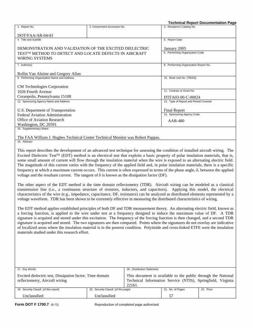
15. Supplementary Notes The FAA William J. Hughes Technical Center Technical Monitor was Robert Pappas. 16. Abstract This report describes the development of an advanced test technique for assessing the condition of installed aircraft wiring. The Excited Dielectric Test™ (EDT) method is an electrical test that exploits a basic property of polar insulation materials, that is, some small amount of current will flow through the insulation material when the wire is exposed to an alternating electric field. The magnitude of this current varies with the frequency of the applied field and, in polar insulation materials, there is a specific frequency at which a maximum current occurs. This current is often expressed in terms of the phase angle, δ, between the applied voltage and the resultant current. The tangent of δ is known as the dissipation factor (DF). The other aspect of the EDT method is the time domain reflectometry (TDR). Aircraft wiring can be modeled as a classical transmission line (i.e., a continuous structure of resistors, inductors, and capacitors). Applying this model, the electrical characteristics of the wire (e.g., impedance, capacitance, DF, resistance) can be analyzed as distributed elements represented by a voltage waveform. TDR has been shown to be extremely effective in measuring the distributed characteristics of wiring. The EDT method applies established principles of both DF and TDR measurement theory. An alternating electric field, known as a forcing function, is applied to the wire under test at a frequency designed to induce the maximum value of DF. A TDR signature is acquired and stored under this excitation. The frequency of the forcing function is then changed, and a second TDR signature is acquired and stored. The two signatures are then compared. Points where the signatures do not overlay are indicative of localized areas where the insulation material is in the poorest condition. Polyimide and cross-linked ETFE were the insulation materials studied under this research effort. 17. Key Words

Excited dielectric test, Dissipation factor, Time domain reflectometry, Aircraft wiring

18. Distribution Statement

This document is available to the public through the National Technical Information Service (NTIS), Springfield, Virginia 22161.

19. Security Classif. (of this report)

Unclassified

20. Security Classif. (of this page)

Unclassified

21. No. of Pages

57

22. Price

Form DOT F 1700.7 (8-72) Reproduction of completed page authorized

ACKNOWLEDGMENTS

CM Technologies would like to thank the management of AirTran Airways for their support of this Federal Aviation Administration sponsored research. In particular, we would like to acknowledge the personal efforts of Mr. Chris Nichols of the AirTran Airways Engineering Group for his help in securing access to a DC9 test aircraft for use as a test bed during the field validation phase of this project.

iii/iv

TABLE OF CONTENTS

Page EXECUTIVE SUMMARY xi 1. INTRODUCTION 1-1

2. THEORY 2-1

2.1 Modeling Aircraft Wiring as a Transmission Line 2-1 2.2 Physics of a Capacitor 2-2 2.3 Material Changes and Dissipation Factor 2-4 2.4 Time Domain Reflectometry and Distributed Impedance 2-5 2.5 Merging TDR and Dissipation Factor Manipulation 2-6 2.6 Implementation of Theory 2-8

2.6.1 Coupling Requirements and Design Details 2-9 2.6.2 Forcing Function Source Considerations 2-10 2.6.3 Time Domain Reflectometry Instrument Considerations 2-10

3. EVALUATION OF COMMERCIALLY AVAILABLE EQUIPMENT 3-1

3.1 Coupling Network 3-1 3.2 Forcing Function Sources 3-2

3.2.1 Hewlett-Packard LF Impedance Analyzer, Model 4192A 3-2 3.2.2 Tabor Electronics Model 8020 Programmable Function Generator 3-2

3.3 Time Domain Reflectometers 3-2

3.3.1 Agilent 54754A TDR Module 3-2 3.3.2 CM Technologies PCI-3100 TDR 3-3 3.3.3 Final Equipment Configuration 3-3

4. WIRE SAMPLE SELECTION, CONDITIONING, AND TESTING 4-1

4.1 Wire Sample Test Fixture 4-1 4.2 Initial Testing 4-3 4.3 Conditioning of Wire Samples 4-4

4.3.1 Nonbreached Samples 4-4 4.3.2 Polyimide Control 4-5 4.3.3 Polyimide Thermally Conditioned 4-7 4.3.4 Polyimide Conditioned With Tap Water 4-8 4.3.5 Polyimide Conditioned With Natural Saltwater 4-8 4.3.6 Polyimide Conditioned With Jet Fuel 4-8

v

4.3.7 Polyimide Conditioned With Hydrazine 4-9 4.3.8 Polyimide Conditioned by Boiling in Water 4-9 4.3.9 Cross-Linked ETFE Conditioned in Water 4-10 4.3.10 Cross-Linked ETFE Conditioned in Saltwater 4-10 4.3.11 Cross-Linked ETFE Conditioned in Jet Fuel 4-11

5. FIELD TESTS 5-1

5.1 First Field Test—PCI-3100 TDR 5-1 5.2 Second Field Test—Aglient 54754A TDR 5-4

6. VALIDATION 6-1

6.1 Requirements for Validation 6-1 6.2 Validation Details 6-1 6.3 Validation Test 6-6 6.4 Data Analysis 6-6 6.5 Results Summary 6-9 6.6 Supplemental Tests and Analysis 6-10

7. CONCLUSIONS AND RECOMMENDATIONS 7-1

APPENDIX A—SENSITIVITY OF TDR TO CABLE DEFECTS CAUSED BY SIMULATED ARC FAULTS

vi

LIST OF FIGURES

Figure Page 2-1 Incremental Components of a Real Transmission Line 2-1

2-2 Incremental Components of a Lossless Transmission Line 2-2

2-3 Current vs Voltage in a Capacitor 2-3

2-4 Dissipation Factor vs Frequency in Polar and Nonpolar Materials 2-4

2-5 Functional Block Diagram of a TDR System 2-5

2-6 General TDR Responses for Resistive Loads 2-6

2-7 Time Domain Reflectometry Signature of a Degraded Portion of an Insulated Wire 2-7

2-8 Time Domain Reflectometry Signature of a Degraded Wire at Frequency F2 2-8

2-9 Comparison of TDR Signatures of Degraded Wire at Frequencies F1 and F2 2-8

2-10 A Basic EDT Coupling Network 2-9

3-1 Sample TDR Signature With and Without Filter Network 3-1

3-2 Final Test Configuration 3-4

3-3 Prototype EDT System in Use in the Field 3-4

4-1 The EDT Test Fixture 4-1

4-2 Grounding Connection Used With all Enclosures 4-2

4-3 Inside Enclosure 1 4-2

4-4 Results of EDT Applied to a Conditioned Coaxial Cable 4-4

4-5 Excited Dielectric Test Results From the Polyimide Control Sample 4-5

4-6 Excited Dielectric Test Results Acquired Using Different Forcing Functions 4-6

4-7 Excited Dielectric Test Results From Polyimide Control Sample Using Forcing Functions of Different Amplitude 4-7

4-8 Results From a Thermally Conditioned Polyimide Sample 4-8

vii

4-9 Time Domain Reflectometry Signatures at 200 MHz, 2 Hz, and 20 Hz of Hydrazine-Conditioned Polyimide 4-9

4-10 Excited Dielectric Test Signatures of Boiled Polyimide 4-10

4-11 Signature of Cross-Linked ETFE Conditioned in Jet Fuel 4-11

4-12 Zoom of Middle Section of Jet Fuel-Conditioned Sample 4-12

5-1 Excited Dielectric Test Signatures of the Left Inboard Wheel Speed Transducer 5-2

5-2 Excited Dielectric Test Signatures of the Left Inboard Transducer 5-3

5-3 Excited Dielectric Test Signatures of the End of the Left Inboard Transducer Circuit 5-3

6-1 Validation Testing at the FAA William J. Hughes Technical Center 6-1

6-2 Polyimide Sample 1—Unconditioned Section 6-3

6-3 Polyimide Sample 3—Abraded not Through Electrically, not Contaminated 6-3

6-4 Polyimide Sample 5—Abraded Through to Conductor, Saltwater Contaminated 6-3

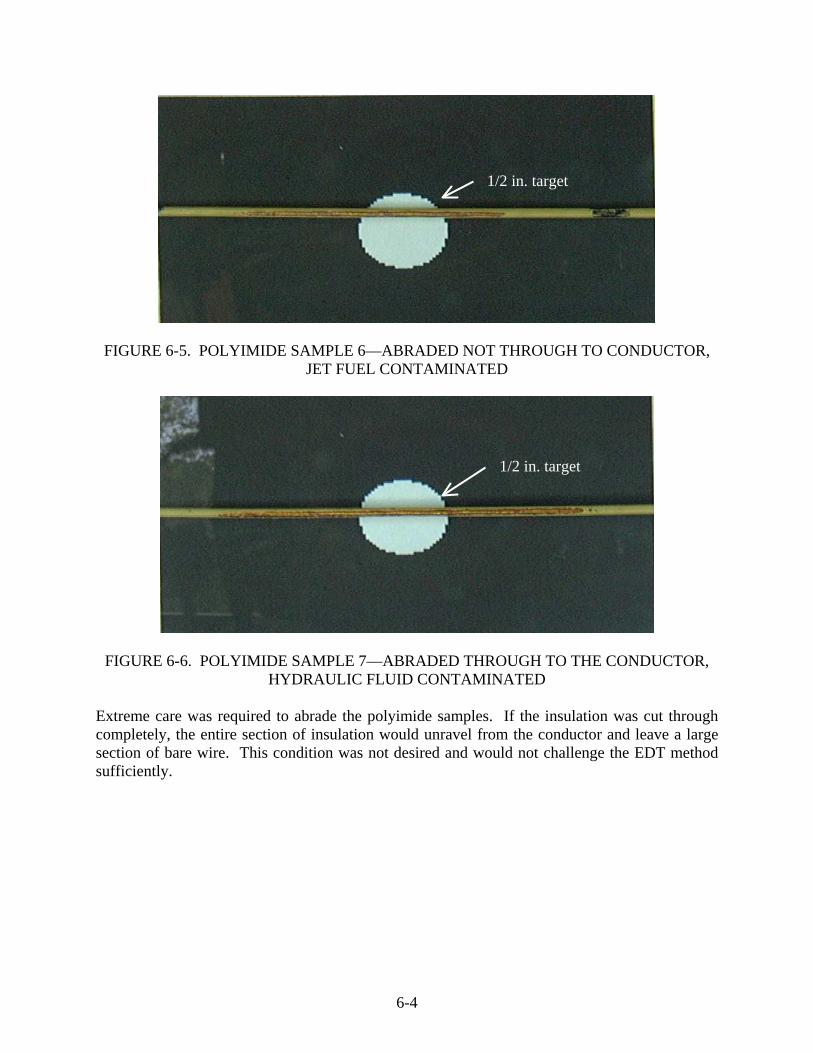
6-5 Polyimide Sample 6—Abraded not Through to Conductor, Jet Fuel Contaminated 6-4

6-6 Polyimide Sample 7—Abraded Through to the Conductor, Hydraulic Fluid Contaminated 6-4

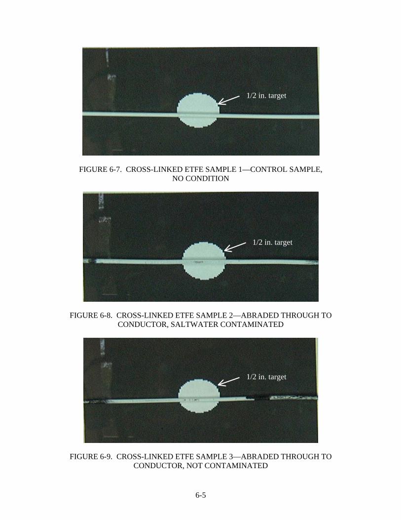
6-7 Cross-Linked ETFE Sample 1—Control Sample, No Condition 6-5

6-8 Cross-Linked ETFE Sample 2—Abraded Through to Conductor, Saltwater Contaminated 6-5

6-9 Cross-Linked ETFE Sample 3—Abraded Through to Conductor, not Contaminated 6-5

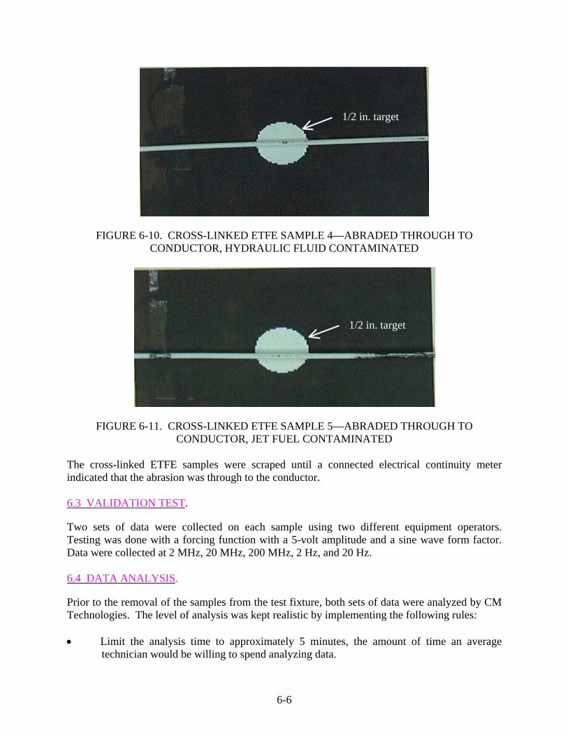
6-10 Cross-Linked ETFE Sample 4—Abraded Through to Conductor, Hydraulic Fluid Contaminated 6-6

6-11 Cross-Linked ETFE Sample 5—Abraded Through to Conductor, Jet Fuel Contaminated 6-6

6-12 Results From Supplemental Test 1 6-10

6-13 Results From Supplemental Test 2 6-11

viii

LIST OF TABLES

Table Page 5-1 Systems and Components Tested on DC-9 5-1 6-1 Sample Numbers and Installed Conditions Used for Final Validation 6-2 6-2 Results of the Blind Analysis 6-7 6-3 Correlation of Sample Letters to Sample Numbers 6-8 6-4 Analysis Results for Distance From the Test Connection to the Condition 6-8

ix

LIST OF ACRONYMS AND SYMBOLS

ac Alternating current C Capacitance c Speed of light CM CM Technologies Corporation dx Incremental length EDT Excited Dielectric Test EMT Electromagnetic tubing ETFE Ethylene-tetrafluoroethylene FAA Federal Aviation Administration G Conductance GPIB General-purpose information bus L Inductance R Resistance TDR Time domain reflectometry Vp Velocity of propagation ZT Load impedance

x

EXECUTIVE SUMMARY

In October 2000, the Federal Aviation Administration (FAA), as part of the Aging Aircraft Research Program, contracted with CM Technologies Corporation to develop an advanced electrical test method to assess the condition of installed aircraft wiring. One of the FAA’s goals under this program was to validate advanced test methods that could be used in the commercial aviation industry to detect the presence of damaged or defective wire insulation. Of specific interest to the FAA and industry are test methods that can be used to detect the presence of nicked and chafed insulation. This report describes the development of an advanced test technique for assessing the condition of installed aircraft wiring. The Excited Dielectric Test™ (EDT) method is an electrical test that exploits a basic property of polar insulation materials, that is, some small amount of current will flow through the insulation material when the wire is exposed to an alternating electric field. The magnitude of this current varies with the frequency of the applied field and, in polar insulation materials, there is a specific frequency at which a maximum current occurs. This current is often expressed in terms of the phase angle, δ, between the applied voltage and the resultant current. The tangent of δ is known as the dissipation factor (DF). The other aspect of the EDT test method is the time domain reflectometry (TDR). Aircraft wiring can be modeled as a classic transmission line (i.e., a continuous structure of resistors, inductors, and capacitors). By applying this model, the electrical characteristics of the wire (e.g., impedance, capacitance, DF, resistance) can be analyzed as distributed elements. TDR has been shown to be extremely effective in measuring the distributed characteristics of wiring. The EDT method applies established principles of both DF and TDR measurement theory. An alternating electric field, known as a forcing function, is applied to the wire under test at a frequency designed to induce the maximum DF. A TDR signature is acquired and stored under this excitation. The frequency of the forcing function is then changed and a second TDR signature is acquired and stored. The two signatures are then compared. Points where the signatures do not overlay represent areas of weak insulation. Polyimide and cross-linked ethylene-tetrafluoroethylene were the insulation materials studied under this research effort. The underlying theory associated with the EDT method was validated in the laboratory and in the field. The EDT was demonstrated to be effective in detecting and locating common defects that may be present in aircraft wiring systems, including abrasions, fluid contamination, and thermal degradation.

xi/xii

1. INTRODUCTION.

In April 2000, the Federal Aviation Administration (FAA) issued a Broad Agency Announcement to support the development of testing and inspection systems, technology, and techniques that characterize and identify material flaws in aircraft wiring. In response, CM Technologies Corporation (CM) proposed the development of a new inspection technology, known as the Excited Dielectric Test™ (EDT) method. CM’s original proposal postulated that the value of lumped impedance associated with a material flaw in aircraft wiring could be purposely altered (i.e., forced to increase or decrease) using an alternating current (ac) stimulus or an electrical forcing function. Furthermore, if the impedance of a material flaw were altered during a time domain reflectometery (TDR) test, it was postulated that the material flaw would appear more pronounced on the resultant TDR waveform (signature). This report describes the research sponsored by the FAA, including • a discussion of the theoretical basis associated with the EDT • the results of an industry survey of suitable test hardware • a summary of the test results from a laboratory testing matrix

1-1/1-2

2. THEORY.

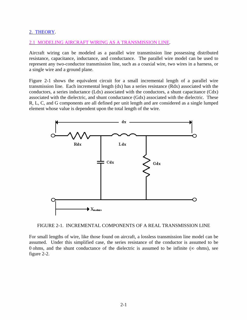
2.1 MODELING AIRCRAFT WIRING AS A TRANSMISSION LINE.

Aircraft wiring can be modeled as a parallel wire transmission line possessing distributed resistance, capacitance, inductance, and conductance. The parallel wire model can be used to represent any two-conductor transmission line, such as a coaxial wire, two wires in a harness, or a single wire and a ground plane. Figure 2-1 shows the equivalent circuit for a small incremental length of a parallel wire transmission line. Each incremental length (dx) has a series resistance (Rdx) associated with the conductors, a series inductance (Ldx) associated with the conductors, a shunt capacitance (Cdx) associated with the dielectric, and shunt conductance (Gdx) associated with the dielectric. These R, L, C, and G components are all defined per unit length and are considered as a single lumped element whose value is dependent upon the total length of the wire.

FIGURE 2-1. INCREMENTAL COMPONENTS OF A REAL TRANSMISSION LINE For small lengths of wire, like those found on aircraft, a lossless transmission line model can be assumed. Under this simplified case, the series resistance of the conductor is assumed to be 0 ohms, and the shunt conductance of the dielectric is assumed to be infinite (∞ ohms), see figure 2-2.

2-1

FIGURE 2-2. INCREMENTAL COMPONENTS OF A LOSSLESS TRANSMISSION LINE The inductance, (Ldx), is a function of the physical properties of the wire and, for installed wiring, can be assumed to be constant. The capacitance of a wire, (Cdx), is a function of geometry, the insulation materials, and the presence of any contamination. For example, consider an insulated wire and a ground plane (the airframe). The insulated wire and airframe form a parallel plate capacitor where the wire’s conductor represents one of the plates, the ground plane or airframe serves as the other plate, and the wire’s insulation acts as the capacitor’s dielectric media. Considering that a wire’s insulation material is directly exposed to the environment and is most susceptible to service wear or accidental damage, capacitance is the electrical parameter of greatest interest in the model shown in figure 2-2. 2.2 PHYSICS OF A CAPACITOR.

A capacitor stores electrical energy in the dielectric by aligning the charge distribution of its molecules in one direction. This alignment is caused when an applied electric field is placed across the plates of the capacitor. While this molecular alignment is being made, a current supplied by a source, such as a battery, flows between the plates and through the capacitor. The magnitude of this current, known as absorption current, is initially very large and decays to practically zero in a period of time that is exponentially proportional to the loop resistance of the circuit and the value of the capacitor. In an ideal capacitor, the absorption current will decay to exactly zero when the voltage of the capacitor equals the voltage of the source and no current flows through the dielectric. When an electric field is applied and as the absorption current deposits charge in the capacitor, the voltage across the capacitor plates will increase to source voltage and the absorption current will decrease to its minimum value. Because the current flows before the voltage builds, it is said that the current leads the voltage in a capacitor. In a pure capacitor, the current would lead the voltage by exactly 90°. Figure 2-3 shows a graph of the voltage and current for a capacitor. In the ideal case, the red vector would overlay on the vertical axis indicating a 90° phase angle.

2-2

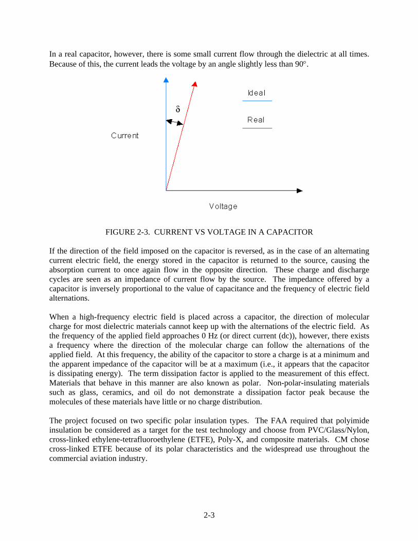
In a real capacitor, however, there is some small current flow through the dielectric at all times. Because of this, the current leads the voltage by an angle slightly less than 90°.

FIGURE 2-3. CURRENT VS VOLTAGE IN A CAPACITOR

If the direction of the field imposed on the capacitor is reversed, as in the case of an alternating current electric field, the energy stored in the capacitor is returned to the source, causing the absorption current to once again flow in the opposite direction. These charge and discharge cycles are seen as an impedance of current flow by the source. The impedance offered by a capacitor is inversely proportional to the value of capacitance and the frequency of electric field alternations. When a high-frequency electric field is placed across a capacitor, the direction of molecular charge for most dielectric materials cannot keep up with the alternations of the electric field. As the frequency of the applied field approaches 0 Hz (or direct current (dc)), however, there exists a frequency where the direction of the molecular charge can follow the alternations of the applied field. At this frequency, the ability of the capacitor to store a charge is at a minimum and the apparent impedance of the capacitor will be at a maximum (i.e., it appears that the capacitor is dissipating energy). The term dissipation factor is applied to the measurement of this effect. Materials that behave in this manner are also known as polar. Non-polar-insulating materials such as glass, ceramics, and oil do not demonstrate a dissipation factor peak because the molecules of these materials have little or no charge distribution. The project focused on two specific polar insulation types. The FAA required that polyimide insulation be considered as a target for the test technology and choose from PVC/Glass/Nylon, cross-linked ethylene-tetrafluoroethylene (ETFE), Poly-X, and composite materials. CM chose cross-linked ETFE because of its polar characteristics and the widespread use throughout the commercial aviation industry.

2-3

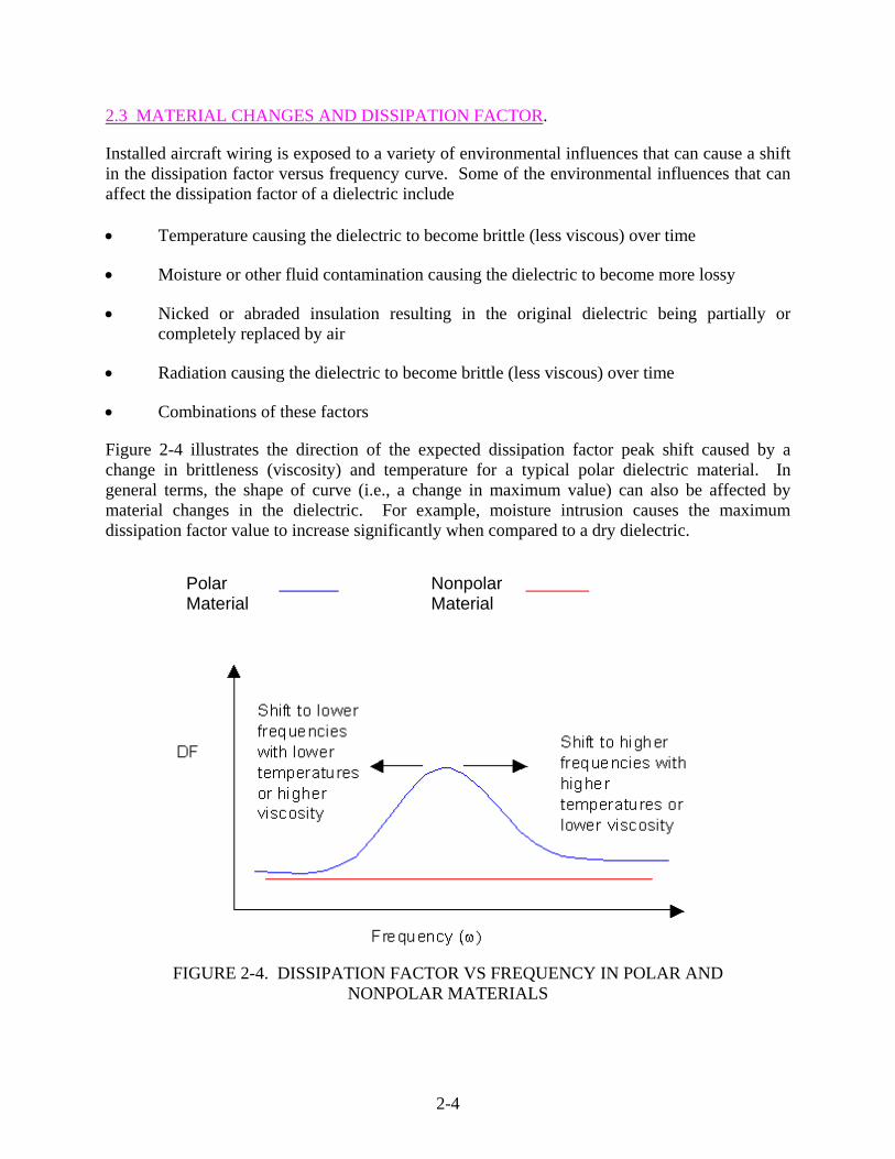
2.3 MATERIAL CHANGES AND DISSIPATION FACTOR.

Installed aircraft wiring is exposed to a variety of environmental influences that can cause a shift in the dissipation factor versus frequency curve. Some of the environmental influences that can affect the dissipation factor of a dielectric include • Temperature causing the dielectric to become brittle (less viscous) over time

• Moisture or other fluid contamination causing the dielectric to become more lossy

• Nicked or abraded insulation resulting in the original dielectric being partially or completely replaced by air

• Radiation causing the dielectric to become brittle (less viscous) over time

• Combinations of these factors

Figure 2-4 illustrates the direction of the expected dissipation factor peak shift caused by a change in brittleness (viscosity) and temperature for a typical polar dielectric material. In general terms, the shape of curve (i.e., a change in maximum value) can also be affected by material changes in the dielectric. For example, moisture intrusion causes the maximum dissipation factor value to increase significantly when compared to a dry dielectric.

Polar Material

Nonpolar Material

FIGURE 2-4. DISSIPATION FACTOR VS FREQUENCY IN POLAR AND NONPOLAR MATERIALS

2-4

2.4 TIME DOMAIN REFLECTOMETRY AND DISTRIBUTED IMPEDANCE.

As discussed earlier, aircraft and other types of wiring are unique circuit elements in that they have both lumped (i.e., capacitance and dissipation factor) and distributed electrical characteristics. TDR is a well-established measurement technique that can be used to determine the distributed electrical proprieties of a wire. Appendix A shows the results of time domain reflectometer sensitivity test. A typical TDR measurement employs a step generator and an oscilloscope in a system best described as a closed-loop radar. A voltage step is injected into the wire under test, and the incident and reflected voltage waves are monitored by the oscilloscope at a particular point on the wire. TDR reveals at a glance the distributed characteristic impedance of the wire, and it shows both the position and the nature (i.e., resistive, capacitive, or inductive) of each discontinuity, or defect, within the wire. A typical TDR setup is shown in figure 2-5.

Pulse Generator

Oscilloscope

Er

ZT

FIGURE 2-5. FUNCTIONAL BLOCK DIAGRAM OF A TDR SYSTEM

The pulse generator produces a positive going pulse, Ei, which is applied to the wire under test. The incident voltage pulse Ei travels down the wire at the velocity of propagation (Vp) that is associated with the wire under test. Vp is a function of several physical characteristics of the wire including: • the dielectric constant of the insulation; • the geometry of the wire (i.e., coaxial, multiconductor, shielded twisted pair); • and the spacing between conductors. The maximum theoretical value of Vp is the speed of light (c). As a practical matter, most aircraft wires have a Vp ranging from 50% c to 80% c. If the load impedance, ZT, is equal to the characteristic impedance of the wire, all of the incident pulse are absorbed by the load impedance and no reflection occurs. If ZT is not equal to the characteristic impedance of the wire under test, a portion of the incident pulse, Ei, will be absorbed and a portion will be reflected, Er.

2-5

The ratio of the incident and reflected voltage waveforms is used to determine the efficiency of the transmission line (i.e., how effective is the wire in transmitting energy from the source to the load). This ratio is called the voltage reflection coefficient, or ρ, and is calculated by taking the ratio of the magnitude of the reflected voltage pulse and the magnitude of the incident voltage pulse, see equation 2-1. ρ = Reflected voltage (Er) / Incident voltage (Ei) = (ZT – Zo)/ (ZT + Zo) (2-1) ρ varies from -1 for a wire terminated with zero impedance (short circuit) to +1 for a wire terminated with infinite impedance (open circuit). Some general TDR responses for various values of ZT are shown in figure 2-6.

FIGURE 2-6. GENERAL TDR RESPONSES FOR RESISTIVE LOADS

2.5 MERGING TDR AND DISSIPATION FACTOR MANIPULATION.

EDT is based on the combination of TDR and dissipation factor manipulation. If an ac forcing function is applied to a wire pair (i.e., single wire and airframe, multiple wires in a harness), the dissipation factor amplitude can be controlled by varying the frequency of the forcing function. This assertion is based on the frequency dependence of the dissipation factor for polar insulation

2-6

materials such as polyimide insulation. TDR is sensitive to changes in capacitance and dissipation factor. An increase or decrease in the dissipation factor will produce an area of decreased or increased impedance in the area of the poorest quality capacitor, or section of wire. In the example shown in figure 2-7, the wire under test is a single conductor and a ground plane. The wire has an area of localized degradation—the nondegraded sections are shown in black, and the degraded section is shown in red. The ground plane is shown in green.

FIGURE 2-7. TIME DOMAIN REFLECTOMETRY SIGNATURE OF A DEGRADED PORTION OF AN INSULATED WIRE

If a section of this wire were degraded (e.g., aged, or exposed to a harsh environment), the dissipation factor peak for this section will occur at a different frequency when compared to the nondegraded portions of the wire. That is, the normal and degraded sections of this wire will appear as having different impedances to a certain excitation frequency (F1). If a TDR test was performed while an excitation signal of frequency F1 is applied, the difference in the dissipation factor will be seen as an area of increased impedance in the TDR signature. The TDR test sees the wire as a transmission line with three characteristic impedances with the degraded area appearing as an outlier. As a practical matter with just a single TDR signature, it would be difficult to determine if the difference in impedance in the degraded section was due to a defector flaw, or if the difference is related to some other factor (i.e., the spacing between the wire and the airframe). For this to be known, a baseline TDR signature would be needed for comparison. Figure 2-8 shows the TDR signature from the same wire with a forcing function applied at a frequency F2, where F2>F1. At frequency F2, the apparent impedances of the normal and degraded sections change, but in opposite directions. The normal sections become better quality capacitors at F2 (the dissipation factor moves away from the peak value), and the degraded section becomes a poorer quality capacitor (the dissipation factor approaches the peak value).

2-7

FIGURE 2-8. TIME DOMAIN REFLECTOMETRY SIGNATURE OF A DEGRADED WIRE AT FREQUENCY F2

Figure 2-9 shows a comparison of the two TDR signatures acquired at forcing function frequencies F1 and F2. The difference of impedance between the two signatures indicates the location of the degraded section. These figures are general for illustrative purposes and are not to scale. Experience and observations suggest that the differences in impedance are, in reality, much more subtle.

FIGURE 2-9. COMPARISON OF TDR SIGNATURES OF DEGRADED WIRE AT FREQUENCIES F1 AND F2

2.6 IMPLEMENTATION OF THEORY.

Implementation of EDT technique requires that two different electrical waveforms, a TDR pulse and an ac forcing function, be applied to the wire under test simultaneously.

2-8

The ac forcing function, which provides the excitation of the dielectric, is a low-frequency ac waveform with a frequency range of 1 MHz to 100 Hz—the frequency range is important because the naturally occurring peak dissipation factor for polyimide and cross-linked ETFE insulation falls within this range. Also, it was assumed that this frequency range was sufficient to bound a shift in peak dissipation factor caused by the degradation mechanisms considered in this project (e.g., fluid contamination, abrasions). The TDR pulse should be a fast risetime, step-function pulse as opposed to another pulse type such as a half-sine pulse. A step-function pulse provides the best horizontal (distance) resolution compared to other pulse types. In addition, because a step pulse is composed of a series of sine waves, the frequency content of a step pulse is very broad. It was assumed that by providing a broadband TDR signal, the probability of detecting subtle defects in a wire’s insulation would be maximized. To apply the ac forcing function and TDR waveform simultaneously, a coupling network is needed. The EDT coupler must be able to pass both the low-frequency forcing function and the high-frequency TDR pulse with minimal loss and attenuation. 2.6.1 Coupling Requirements and Design Details.

Ideally, the EDT coupling device will: • allow a low-frequency ac signal, the forcing function, to pass,

• protect the TDR instrument from seeing the forcing function source so that the waveform is not adversely affected,

• provide the largest bandwidth for the TDR to realize the greatest resolution, and

• permit the two-way travel of the TDR pulse without attenuation.

CM chose an LC “T” filter network composed of a capacitor and an inductor for the EDT coupling device. Figure 2-10 shows the basic configuration of the coupling network.

FIGURE 2-10. A BASIC EDT COUPLING NETWORK

2-9

2.6.2 Forcing Function Source Considerations.

As mentioned earlier, the forcing function source is required to provide an ac waveform with frequencies ranging from 1 MHz to 100 Hz. This frequency range was selected to be bounding. In other words, the forcing function source needed sufficient range to excite the dielectric at or near the natural peak dissipation factor frequency. As a question to be researched, the amplitude and form factor of the forcing function should be selectable. To protect the TDR and to limit the power delivered to the wire under test, the amplitude should be adjustable from 0 to 5 volts. To investigate the effect that the forcing function form factor has on a wire sample, the source is required to supply a sine wave, a sawtooth wave, a square wave, and pulse trains. 2.6.3 Time Domain Reflectometry Instrument Considerations.

Some of the important considerations for the TDR instrument include: • The TDR is required to be a digital system to allow the digital representation of the

signatures. This is necessary because several signatures are to be overlaid to detect subtle differences in impedance.

• The TDR is required to have sufficient resolution at wire lengths found in commercial

aircraft, up to 1000 feet (approximately 300 m). • The electrical energy the TDR pulse delivers to the circuit under test is required to be

very small. This is an important consideration given the environments that wires are subjected to in a commercial aircraft and the thickness of the insulation. For example, if a nicked wire were installed in a fuel tank, the energy of the TDR pulse would need to be adjustable to evaluate the wire in a safe manner.

2-10

3. EVALUATION OF COMMERCIALLY AVAILABLE EQUIPMENT.

3.1 COUPLING NETWORK.

Several options were considered for coupling the TDR pulse and the ac forcing function onto the wire under test. Beyond the basic desired performance characteristics size, weight, ruggedness, availability, and the ability to withstand voltage were also considered. CM felt that the Picosecond Pulse Laboratory, Bias Tee Network, Model 5541A, was the best choice for this project. This coupling network passed the forcing function and the TDR pulse efficiently. The network adds a noticeable amount of series impedance to the circuit under test. For the purposes of this project, however, this added impedance is not a problem because only a qualitative, not quantitative, indication of impedance is required. Figure 3-1 shows the performance of the selected filter network. The cyan trace shows the TDR signature without the selected coupling network. The green trace is the signature of the same circuit with the coupling network installed. The impedance of the wire under test is not affected by the coupling network.

Impedance of the wire under test is identical except for

resistive offset

Green signature was acquired with the coupling network

Cyan signature was acquired without the coupling network

FIGURE 3-1. SAMPLE TDR SIGNATURE WITH AND WITHOUT FILTER NETWORK

3-1

3.2 FORCING FUNCTION SOURCES.

3.2.1 Hewlett-Packard LF Impedance Analyzer, Model 4192A.

The Hewlett-Packard LF Impedance Analyzer, Model 4192A was investigated as a possible excitation source for several reasons. The 4192A can sweep frequencies from 5 Hz to 13 MHz and acquire impedance data, including dissipation factor. This unit can be programmed to perform swept frequency measurements and can be interfaced with a controller via a general-purpose information bus (GPIB). While the 4192A is very versatile, several limitations precluded this unit from further study. Specifically: • The output waveforms available from the 4192A are limited—only sine waves with

amplitudes up to 1 volt are possible.

• When the instrument was programmed for very low frequencies, 5 to 20 Hz, the resulting impedance measurements were unstable and not repeatable in the laboratory.

• Using the 4192A would require subtracting the impedance values of the coupler from the data. There was a concern that subtle shifts in impedance or dissipation factor may have been masked by the presence of the coupler.

No data presented in this report was collected with the 4192A because repeatability could not be obtained at very low frequencies. 3.2.2 Tabor Electronics Model 8020 Programmable Function Generator.

The Tabor Electronics Model 8020 function generator was ultimately selected for use in this project. The 8020 can source waveforms with frequencies from 2 to 20 MHz with amplitudes as large as 30 volts. The 8020 produces a variety of waveforms, including sine, square, sawtooth, and pulse trains, both negative and positive. The model 8020 also has a GPIB port to allow interfacing with a controller for automated control. All the data that are presented in this report was taken using the Tabor Electronics Model 8020. 3.3 TIME DOMAIN REFLECTOMETERS.

The performance of two TDR instruments was evaluated for this application. Both instruments met the requirement of being digital and allowing comparison of multiple signatures. 3.3.1 Agilent 54754A TDR Module.

The Agilent 54754A is a high-end, laboratory-grade TDR. The system operates under a Windows® operating system and has the ability to store thousands of signatures internally. The

3-2

54754A has an adjustable pulse width to allow testing of various wire lengths ranging from less than 1 inch to several hundred feet long. The 54754A produces a continuous train of output pulses for a real-time measurement. This instrument requires that the user have a certain amount of knowledge about the wire under test in order to adjust the pulse width for the required length. The presentation of the TDR signature is displayed with the horizontal axis in units of time rather than actual distance. Therefore, the user must multiply the measure time by the velocity of propagation of the wire to separately calculate the distance. The software controlling the 54754A has a very convenient zoom feature, which in conjunction with a touchscreen operation, allows rapid zooming in on TDR signatures. The feature, however, will not zoom in or out on stored signatures. An important practical limitation of the 54754A TDR module is its sensitivity to electrostatic damage. A slight static charge induced across the input will destroy the module. Static charges are quite common on installed aircraft wiring, so care needs to be taken when acquiring field data with the 54754A TDR module. 3.3.2 CM Technologies PCI-3100 TDR.

The PCI-3100 TDR is implemented in an ISA expansion card form factor and operates within an IBM®-compatible personal computer. The PCI-3100 can test circuits with lengths up to 3000 feet. The control software allows the user to compare up to eight waveforms, and stores as many signatures as the computer hard drive can accommodate. The PCI-3100 control software can magnify acquired and stored signatures up to 64x in steps of 2 (e.g., 2x, 4x, 8x). The control software also allows manipulation of the velocity of propagation so that an accurate measurement of length can be made between any two points along the waveform. The pulse generator used in the PCI-3100 is very robust. Extensive field use of the PCI-3100 suggests that its pulser, while not as fast as the pulser used in the Agilent 54754A TDR module, is more tolerant of electrostatic discharge. The majority of the data presented in this report were acquired with the PCI-3100 TDR. 3.3.3 Final Equipment Configuration.

Figure 3-2 is a block diagram of the final equipment configuration used in this project. This is the configuration with which all EDT data in this report were obtained.

3-3

FIGURE 3-2. FINAL TEST CONFIGURATION Figure 3-3 shows the prototype EDT equipment (labeled 1-4) used during a field test evaluation. 1. CM Technologies PCI-3100 TDR installed in a field computer

2. Tabor Electronics 8020 function generator

3. Agilent 54754A TDR Module installed in the Agilent Model 86100 Oscilloscope Mainframe

4. Picosecond Pulse Laboratory, Bias Tee Network, Model 5541A

FIGURE 3-3. PROTOTYPE EDT SYSTEM IN USE IN THE FIELD

3-4

4. WIRE SAMPLE SELECTION, CONDITIONING, AND TESTING.

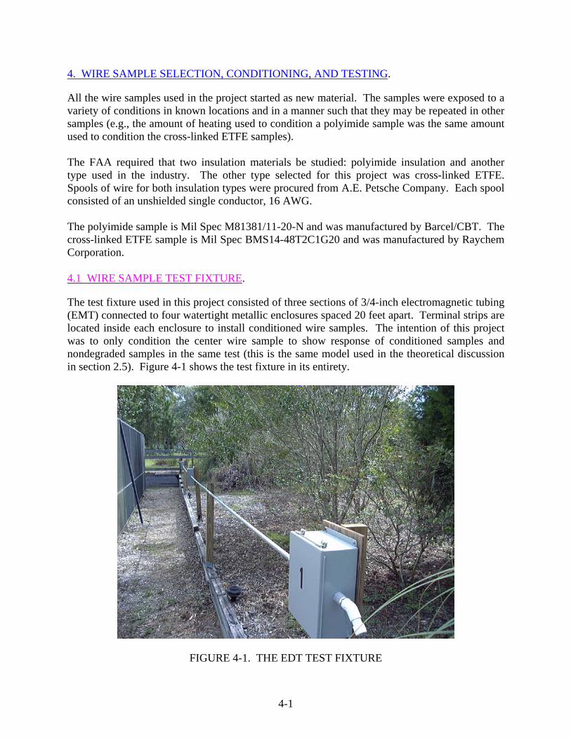
All the wire samples used in the project started as new material. The samples were exposed to a variety of conditions in known locations and in a manner such that they may be repeated in other samples (e.g., the amount of heating used to condition a polyimide sample was the same amount used to condition the cross-linked ETFE samples). The FAA required that two insulation materials be studied: polyimide insulation and another type used in the industry. The other type selected for this project was cross-linked ETFE. Spools of wire for both insulation types were procured from A.E. Petsche Company. Each spool consisted of an unshielded single conductor, 16 AWG. The polyimide sample is Mil Spec M81381/11-20-N and was manufactured by Barcel/CBT. The cross-linked ETFE sample is Mil Spec BMS14-48T2C1G20 and was manufactured by Raychem Corporation. 4.1 WIRE SAMPLE TEST FIXTURE.

The test fixture used in this project consisted of three sections of 3/4-inch electromagnetic tubing (EMT) connected to four watertight metallic enclosures spaced 20 feet apart. Terminal strips are located inside each enclosure to install conditioned wire samples. The intention of this project was to only condition the center wire sample to show response of conditioned samples and nondegraded samples in the same test (this is the same model used in the theoretical discussion in section 2.5). Figure 4-1 shows the test fixture in its entirety.

FIGURE 4-1. THE EDT TEST FIXTURE

4-1

Each metallic enclosure is grounded to a single-point earth ground. Figure 4-2 shows the ground connection on enclosure 1, which is typical of all enclosures.

FIGURE 4-2. GROUNDING CONNECTION USED WITH ALL ENCLOSURES As shown in figure 4-2, the coating of the enclosure mount was removed to bare metal to insure a good, consistent ground. Enclosure 1, as shown in figure 4-3, is the location of the EDT test lead connection (red and black alligator clips) to the wire sample. The inside of enclosure 1 is typical of the other enclosures, with the exception of the convenient ground connection in the lower portion of the panel and the PVC test lead tube. Coating on both sides of the lower right mount hole of all panels was removed to bare metal to insure a good and consistent ground.

FIGURE 4-3. INSIDE ENCLOSURE 1

4-2

4.2 INITIAL TESTING.

The first goal of the project was to demonstrate the basic theory associated with the EDT method. To achieve this goal, the project began with the application of EDT to a cross-linked polyethylene (XLPE) insulated coaxial wire. Coaxial wire was selected as the starting point because it possesses well-understood impedance characteristics and has a uniform geometry. Two 30-foot lengths of coaxial cable were connected together to form the circuit and were installed in the test fixture. The barrel connector used to connect both samples together was insulated from ground so that the shield was floated. The first 30-foot length was not conditioned. The second 30-foot length was conditioned by introducing an abrasion to the wire jacket located approximately 18 inches from the intermediate barrel connector. The EDT was applied between the shield and the ground of the test fixture since this configuration would consider the condition of the jacket material. Figure 4-4 shows the first demonstration of the EDT method. Figure 4-4 is a 32x magnification of the coaxial sample excited at 1 Hz (cyan signature) and 15 Hz (red signature). The green signature was acquired with the coaxial cable open at the intermediate barrel connector to easily locate the end of the first 30-foot length and the location of the connector. • The blue signature was acquired using an excitation frequency of 1 Hz. The red signature

was acquired at 15 Hz.

• Item 1 shows the location of the connection between both samples. This signature was acquired with cable 2 disconnected from cable 1 with no excitation.

• Item 2 shows the location of the connector on cable 1, which was insulated from ground with electrical tape.

• Item 3 shows the location of the connector on cable 2, which was insulated from ground with electrical tape.

• Item 4 shows the location of the beginning of the conditioned area (approximately 18 inches from item 3).

• Item 5 shows the location of the unconditioned areas of the two cables near the connector area.

4-3

FIGURE 4-4. RESULTS OF EDT APPLIED TO A CONDITIONED COAXIAL CABLE

The change in insulation at the connectors is clearly indicated by the difference in impedance seen when using two different forcing function frequencies. The conditioned area is also indicated, although not uniformly. The lack of uniformity is due to the conditioned portion of the cable not lying uniformly with respect to the ground plane. 4.3 CONDITIONING OF WIRE SAMPLES.

Wire degradation was grouped into three general categories: breached insulation that had not become contaminated (i.e., a clean breach), breached insulation that had become contaminated, and nonbreached insulation. The nonbreached wire samples were subjected to conditions and media that were believed to be realistic (e.g., fluids found on commercial aircraft) and would be representative of service wear in an aircraft. Generally, the samples were conditioned until a visible difference (e.g., color change) could be discerned. Breached samples included complete abrasion (abraded through until the conductor became exposed) and partially abraded (the insulation was abraded but the conductor was not exposed). 4.3.1 Nonbreached Samples.

Twenty-foot samples of polyimide and cross-linked ETFE were placed in fluids and conditions to simulate the environments seen by wiring installed on commercial aircraft. The samples were placed in containers so that only the middle 1-foot section of the sample was immersed in the conditioning media.

4-4

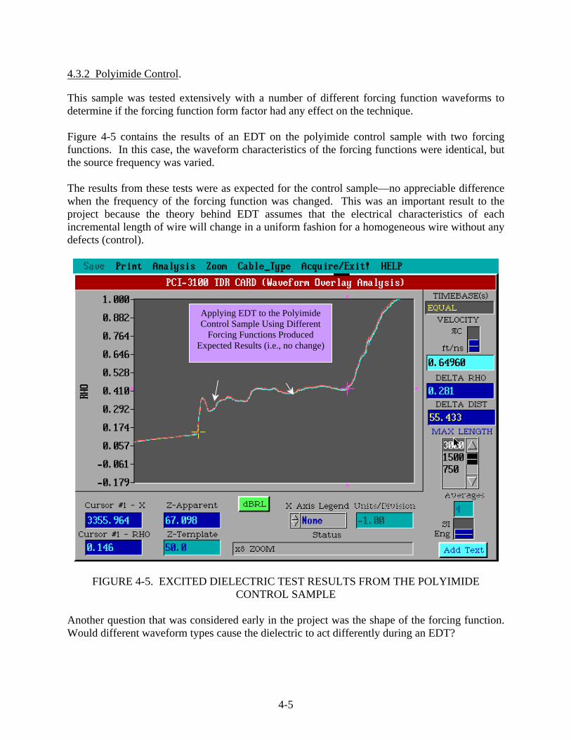
4.3.2 Polyimide Control.

This sample was tested extensively with a number of different forcing function waveforms to determine if the forcing function form factor had any effect on the technique. Figure 4-5 contains the results of an EDT on the polyimide control sample with two forcing functions. In this case, the waveform characteristics of the forcing functions were identical, but the source frequency was varied. The results from these tests were as expected for the control sample—no appreciable difference when the frequency of the forcing function was changed. This was an important result to the project because the theory behind EDT assumes that the electrical characteristics of each incremental length of wire will change in a uniform fashion for a homogeneous wire without any defects (control).

Applying EDT to the Polyimide Control Sample Using Different

Forcing Functions Produced Expected Results (i.e., no change)

FIGURE 4-5. EXCITED DIELECTRIC TEST RESULTS FROM THE POLYIMIDE

CONTROL SAMPLE Another question that was considered early in the project was the shape of the forcing function. Would different waveform types cause the dielectric to act differently during an EDT?

4-5

Figure 4-6 shows an example of the results. Figure 4-6 is a comparison of the four TDR signatures acquired using four different forcing function waveforms: sine wave, sawtooth, positive pulse, and square. All four TDR signatures are identical, suggesting that the shape of the forcing function (i.e., sine, triangle) does not have a significant effect on the EDT results.

The shape of the Forcing Function

waveform had little effect on the

TDR signature

FIGURE 4-6. EXCITED DIELECTRIC TEST RESULTS ACQUIRED USING DIFFERENT

FORCING FUNCTIONS Another variable that was examined during the early stages of the research was the effect, if any, that the amplitude of the forcing function had on the EDT method. Figure 4-7 is a comparison of two EDT signatures: the green signature was acquired with a 1 volt peak-to-peak (Vpp) sine wave forcing function, and the cyan signature was acquired with a 5 Vpp sine wave forcing function. The data suggest that the EDT method is not affected by the amplitude of the forcing function. This was an important finding since there is always a concern regarding the amount of energy placed on an installed wire in an aircraft. Since the amplitude of the forcing function does not appear to influence the EDT results, the energy introduced into the wire can be kept at a minimum.

4-6

The amplitude of the Forcing Function

waveform had little effect on the TDR

signature

FIGURE 4-7. EXCITED DIELECTRIC TEST RESULTS FROM POLYIMIDE CONTROL

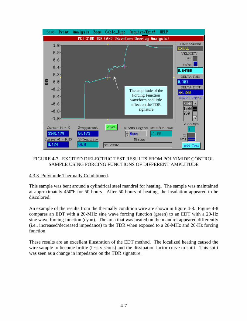
SAMPLE USING FORCING FUNCTIONS OF DIFFERENT AMPLITUDE 4.3.3 Polyimide Thermally Conditioned.

This sample was bent around a cylindrical steel mandrel for heating. The sample was maintained at approximately 450ºF for 50 hours. After 50 hours of heating, the insulation appeared to be discolored. An example of the results from the thermally condition wire are shown in figure 4-8. Figure 4-8 compares an EDT with a 20-MHz sine wave forcing function (green) to an EDT with a 20-Hz sine wave forcing function (cyan). The area that was heated on the mandrel appeared differently (i.e., increased/decreased impedance) to the TDR when exposed to a 20-MHz and 20-Hz forcing function. These results are an excellent illustration of the EDT method. The localized heating caused the wire sample to become brittle (less viscous) and the dissipation factor curve to shift. This shift was seen as a change in impedance on the TDR signature.

4-7

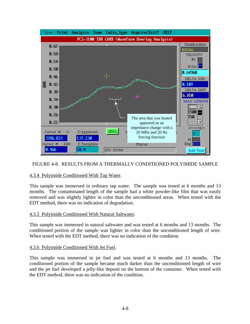
The area that was heated appeared as an

impedance change with a 20 MHz and 20 Hz

forcing function

FIGURE 4-8. RESULTS FROM A THERMALLY CONDITIONED POLYIMIDE SAMPLE

4.3.4 Polyimide Conditioned With Tap Water.

This sample was immersed in ordinary tap water. The sample was tested at 6 months and 13 months. The contaminated length of the sample had a white powder-like film that was easily removed and was slightly lighter in color than the unconditioned areas. When tested with the EDT method, there was no indication of degradation. 4.3.5 Polyimide Conditioned With Natural Saltwater.

This sample was immersed in natural saltwater and was tested at 6 months and 13 months. The conditioned portion of the sample was lighter in color than the unconditioned length of wire. When tested with the EDT method, there was no indication of the condition. 4.3.6 Polyimide Conditioned With Jet Fuel.

This sample was immersed in jet fuel and was tested at 6 months and 13 months. The conditioned portion of the sample became much darker than the unconditioned length of wire and the jet fuel developed a jelly-like deposit on the bottom of the container. When tested with the EDT method, there was no indication of the condition.

4-8

4.3.7 Polyimide Conditioned With Hydrazine.

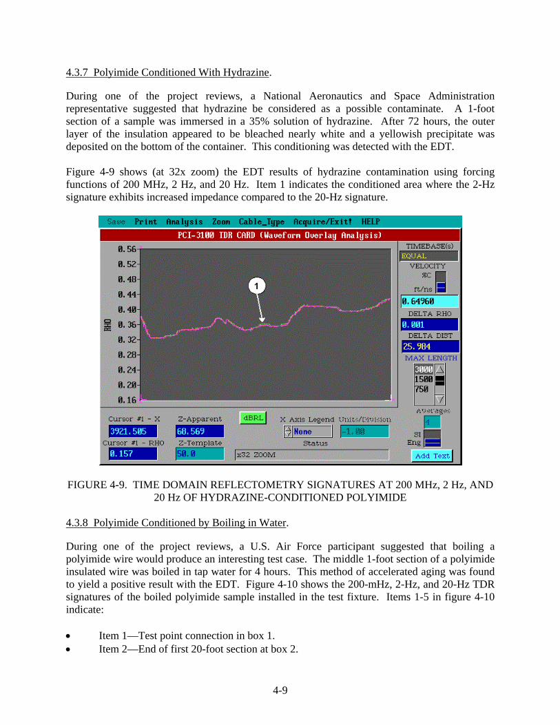
During one of the project reviews, a National Aeronautics and Space Administration representative suggested that hydrazine be considered as a possible contaminate. A 1-foot section of a sample was immersed in a 35% solution of hydrazine. After 72 hours, the outer layer of the insulation appeared to be bleached nearly white and a yellowish precipitate was deposited on the bottom of the container. This conditioning was detected with the EDT. Figure 4-9 shows (at 32x zoom) the EDT results of hydrazine contamination using forcing functions of 200 MHz, 2 Hz, and 20 Hz. Item 1 indicates the conditioned area where the 2-Hz signature exhibits increased impedance compared to the 20-Hz signature.

FIGURE 4-9. TIME DOMAIN REFLECTOMETRY SIGNATURES AT 200 MHz, 2 Hz, AND 20 Hz OF HYDRAZINE-CONDITIONED POLYIMIDE

4.3.8 Polyimide Conditioned by Boiling in Water.

During one of the project reviews, a U.S. Air Force participant suggested that boiling a polyimide wire would produce an interesting test case. The middle 1-foot section of a polyimide insulated wire was boiled in tap water for 4 hours. This method of accelerated aging was found to yield a positive result with the EDT. Figure 4-10 shows the 200-mHz, 2-Hz, and 20-Hz TDR signatures of the boiled polyimide sample installed in the test fixture. Items 1-5 in figure 4-10 indicate: • Item 1—Test point connection in box 1. • Item 2—End of first 20-foot section at box 2.

4-9

• Item 3—Middle of second 20-foot section between boxes 2 and 3. • Item 4—End of second 20-foot section at box 3. • Item 5—End of third 20-foot section at box 4.

FIGURE 4-10. EXCITED DIELECTRIC TEST SIGNATURES OF BOILED POLYIMIDE This figure is only 8x zoom of the signatures. The difference in the low-frequency traces (green 200 MHz, cyan 2 Hz, and red 20 Hz) is very apparent. 4.3.9 Cross-Linked ETFE Conditioned in Water.

A 1-foot section of a cross-linked ETFE sample was immersed in ordinary tap water for 13 months. The sample was new material and had no other defects present. For this reason, the EDT detected no condition. 4.3.10 Cross-Linked ETFE Conditioned in Saltwater.

A 1-foot section of a cross-linked ETFE sample was also soaked in natural saltwater for 13 months. The sample was also new material and had no other defects present. For this reason, the EDT detected no condition in this sample.

4-10

4.3.11 Cross-Linked ETFE Conditioned in Jet Fuel.

A 1-foot section of a cross-linked ETFE sample was immersed in jet fuel for 13 months. Unlike the polyimide sample soaked in jet fuel, EDT detected a condition in the center area of the cross-linked ETFE sample when it was installed in the test fixture. Figure 4-11 is a comparison, at 4x zoom, of the 200-MHz, 2-Hz and 20-Hz signatures of the cross-linked ETFE sample conditioned with jet fuel. Items 1-5 in figure 4-11 indicate: • Item 1—Test connection at box 1. • Item 2—End of first 20-foot section at box 2. • Item 3—Middle of second 20-foot section between boxes 2 and 3. • Item 4—End of second 20-foot section at box 3. • Item 5—End of third 20-foot section at box 4.

FIGURE 4-11. SIGNATURE OF CROSS-LINKED ETFE CONDITIONED IN JET FUEL This condition is visually detectable near item 3 at 4x zoom. The condition becomes more distinct at 32x zoom, see figure 4-12. Items 1 and 2 in figure 4-12 indicate: • Item 1—Indication of condition. • Item 2—End of second 20-foot section at box 3.

4-11

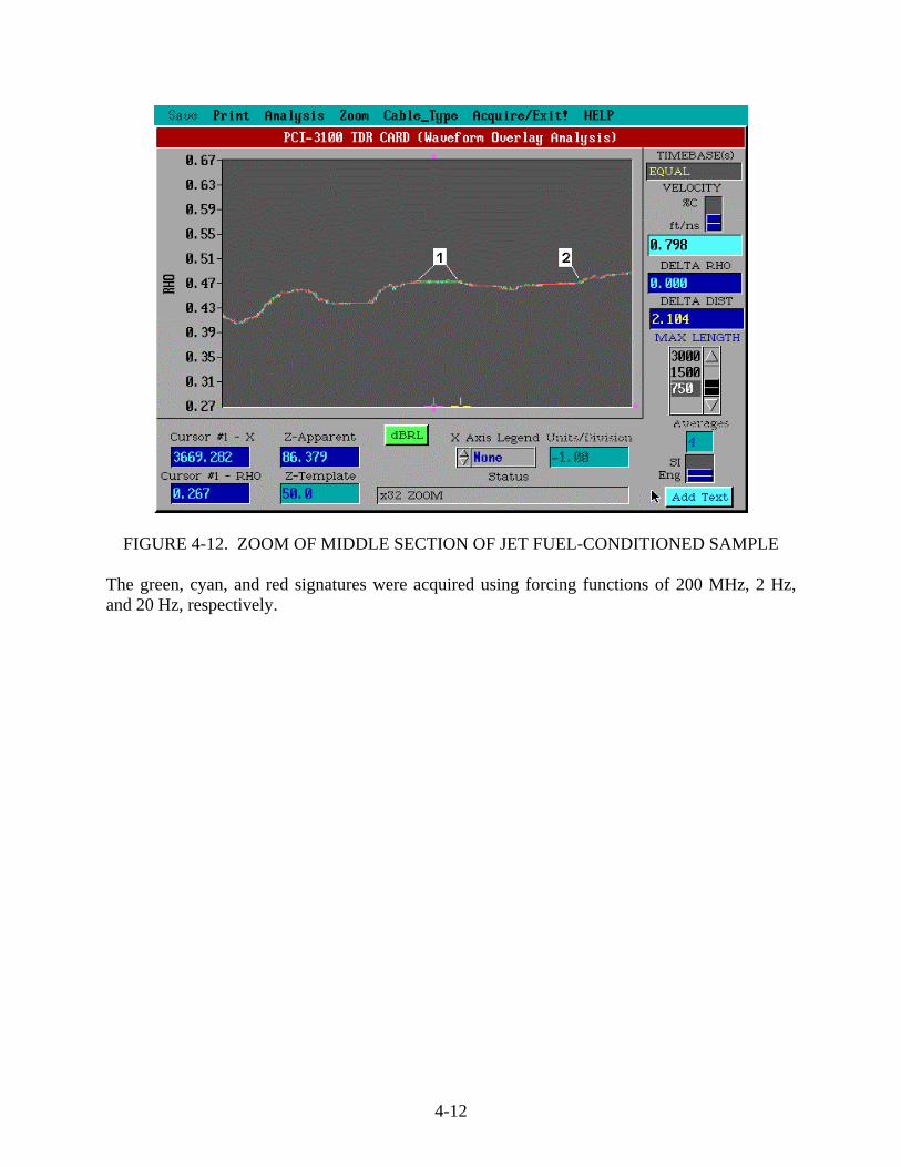
FIGURE 4-12. ZOOM OF MIDDLE SECTION OF JET FUEL-CONDITIONED SAMPLE The green, cyan, and red signatures were acquired using forcing functions of 200 MHz, 2 Hz, and 20 Hz, respectively.

4-12

5. FIELD TESTS.

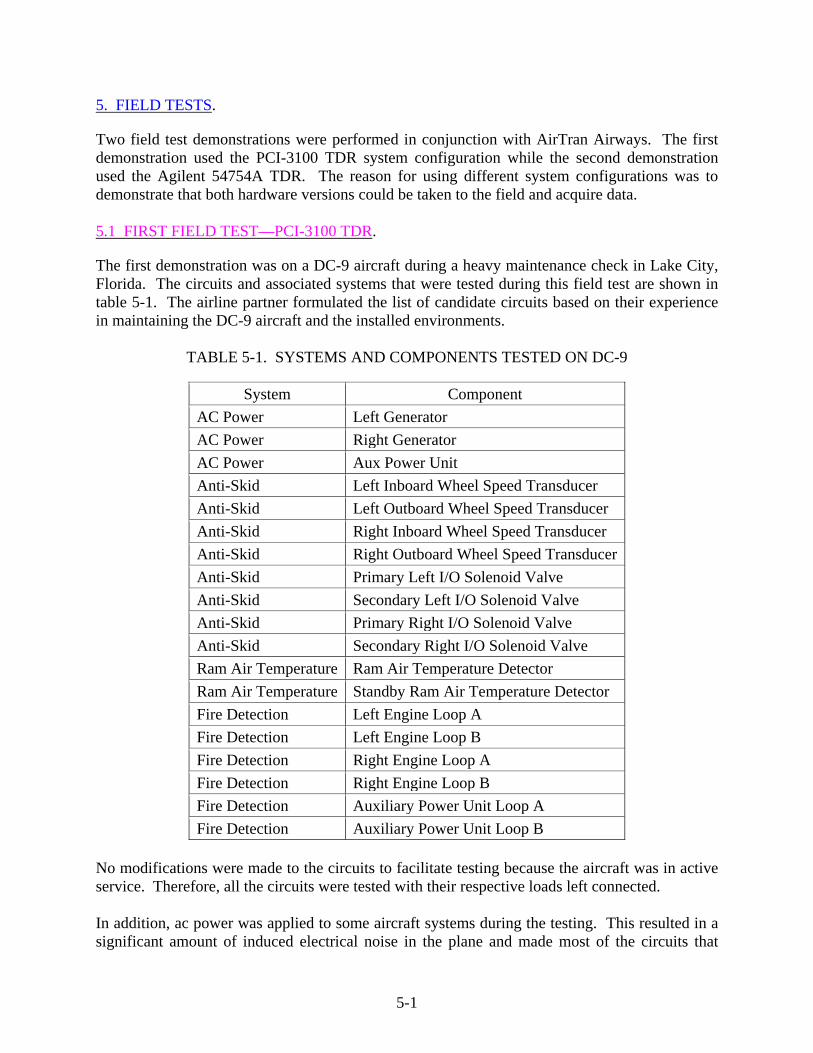
Two field test demonstrations were performed in conjunction with AirTran Airways. The first demonstration used the PCI-3100 TDR system configuration while the second demonstration used the Agilent 54754A TDR. The reason for using different system configurations was to demonstrate that both hardware versions could be taken to the field and acquire data. 5.1 FIRST FIELD TEST—PCI-3100 TDR.

The first demonstration was on a DC-9 aircraft during a heavy maintenance check in Lake City, Florida. The circuits and associated systems that were tested during this field test are shown in table 5-1. The airline partner formulated the list of candidate circuits based on their experience in maintaining the DC-9 aircraft and the installed environments.

TABLE 5-1. SYSTEMS AND COMPONENTS TESTED ON DC-9

System Component AC Power Left Generator AC Power Right Generator AC Power Aux Power Unit Anti-Skid Left Inboard Wheel Speed Transducer Anti-Skid Left Outboard Wheel Speed Transducer Anti-Skid Right Inboard Wheel Speed Transducer Anti-Skid Right Outboard Wheel Speed Transducer Anti-Skid Primary Left I/O Solenoid Valve Anti-Skid Secondary Left I/O Solenoid Valve Anti-Skid Primary Right I/O Solenoid Valve Anti-Skid Secondary Right I/O Solenoid Valve Ram Air Temperature Ram Air Temperature Detector Ram Air Temperature Standby Ram Air Temperature Detector Fire Detection Left Engine Loop A Fire Detection Left Engine Loop B Fire Detection Right Engine Loop A Fire Detection Right Engine Loop B Fire Detection Auxiliary Power Unit Loop A Fire Detection Auxiliary Power Unit Loop B

No modifications were made to the circuits to facilitate testing because the aircraft was in active service. Therefore, all the circuits were tested with their respective loads left connected. In addition, ac power was applied to some aircraft systems during the testing. This resulted in a significant amount of induced electrical noise in the plane and made most of the circuits that

5-1

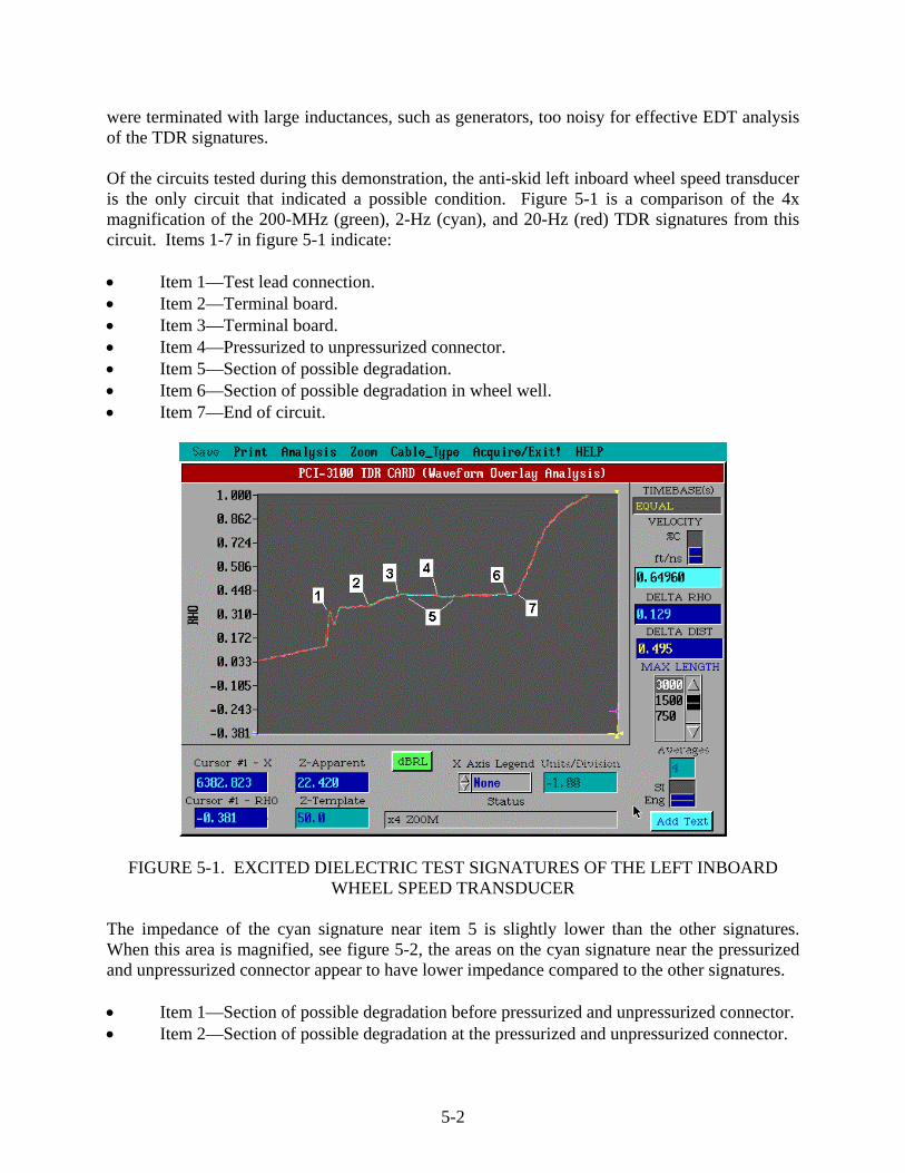
were terminated with large inductances, such as generators, too noisy for effective EDT analysis of the TDR signatures. Of the circuits tested during this demonstration, the anti-skid left inboard wheel speed transducer is the only circuit that indicated a possible condition. Figure 5-1 is a comparison of the 4x magnification of the 200-MHz (green), 2-Hz (cyan), and 20-Hz (red) TDR signatures from this circuit. Items 1-7 in figure 5-1 indicate: • Item 1—Test lead connection. • Item 2—Terminal board. • Item 3—Terminal board. • Item 4—Pressurized to unpressurized connector. • Item 5—Section of possible degradation. • Item 6—Section of possible degradation in wheel well. • Item 7—End of circuit.

FIGURE 5-1. EXCITED DIELECTRIC TEST SIGNATURES OF THE LEFT INBOARD WHEEL SPEED TRANSDUCER

The impedance of the cyan signature near item 5 is slightly lower than the other signatures. When this area is magnified, see figure 5-2, the areas on the cyan signature near the pressurized and unpressurized connector appear to have lower impedance compared to the other signatures. • Item 1—Section of possible degradation before pressurized and unpressurized connector. • Item 2—Section of possible degradation at the pressurized and unpressurized connector.

5-2

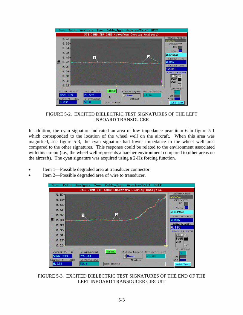
FIGURE 5-2. EXCITED DIELECTRIC TEST SIGNATURES OF THE LEFT INBOARD TRANSDUCER

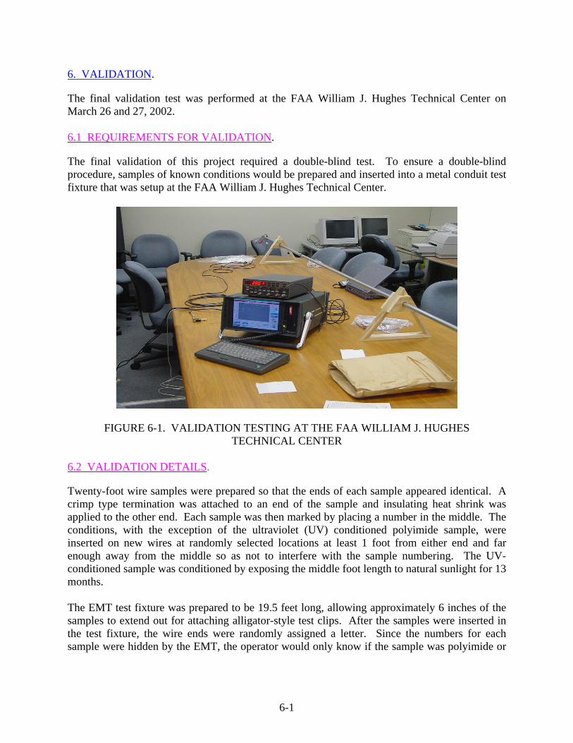
In addition, the cyan signature indicated an area of low impedance near item 6 in figure 5-1 which corresponded to the location of the wheel well on the aircraft. When this area was magnified, see figure 5-3, the cyan signature had lower impedance in the wheel well area compared to the other signatures. This response could be related to the environment associated with this circuit (i.e., the wheel well represents a harsher environment compared to other areas on the aircraft). The cyan signature was acquired using a 2-Hz forcing function. • Item 1—Possible degraded area at transducer connector. • Item 2—Possible degraded area of wire to transducer.

FIGURE 5-3. EXCITED DIELECTRIC TEST SIGNATURES OF THE END OF THE LEFT INBOARD TRANSDUCER CIRCUIT

5-3

5.2 SECOND FIELD TEST—AGLIENT 54754A TDR.

This field testing demonstration was performed with the Agilent 54754A TDR on a DC-9 aircraft that had recently been removed from service and was scheduled to be scrapped. The circuits selected for testing included generator power cables and all of the fuel boost pumps. In general, all the circuits that were tested appeared to be in very good condition, and the real-time analysis performed in the hanger found no areas of degradation. These test files are not included in this report.

5-4

6. VALIDATION.

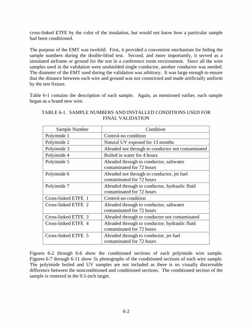
The final validation test was performed at the FAA William J. Hughes Technical Center on March 26 and 27, 2002. 6.1 REQUIREMENTS FOR VALIDATION.

The final validation of this project required a double-blind test. To ensure a double-blind procedure, samples of known conditions would be prepared and inserted into a metal conduit test fixture that was setup at the FAA William J. Hughes Technical Center.

FIGURE 6-1. VALIDATION TESTING AT THE FAA WILLIAM J. HUGHES TECHNICAL CENTER

6.2 VALIDATION DETAILS.

Twenty-foot wire samples were prepared so that the ends of each sample appeared identical. A crimp type termination was attached to an end of the sample and insulating heat shrink was applied to the other end. Each sample was then marked by placing a number in the middle. The conditions, with the exception of the ultraviolet (UV) conditioned polyimide sample, were inserted on new wires at randomly selected locations at least 1 foot from either end and far enough away from the middle so as not to interfere with the sample numbering. The UV-conditioned sample was conditioned by exposing the middle foot length to natural sunlight for 13 months. The EMT test fixture was prepared to be 19.5 feet long, allowing approximately 6 inches of the samples to extend out for attaching alligator-style test clips. After the samples were inserted in the test fixture, the wire ends were randomly assigned a letter. Since the numbers for each sample were hidden by the EMT, the operator would only know if the sample was polyimide or

6-1

cross-linked ETFE by the color of the insulation, but would not know how a particular sample had been conditioned. The purpose of the EMT was twofold. First, it provided a convenient mechanism for hiding the sample numbers during the double-blind test. Second, and more importantly, it served as a simulated airframe or ground for the test in a conference room environment. Since all the wire samples used in the validation were unshielded single conductor, another conductor was needed. The diameter of the EMT used during the validation was arbitrary. It was large enough to ensure that the distance between each wire and ground was not constricted and made artificially uniform by the test fixture. Table 6-1 contains the description of each sample. Again, as mentioned earlier, each sample began as a brand new wire.

TABLE 6-1. SAMPLE NUMBERS AND INSTALLED CONDITIONS USED FOR FINAL VALIDATION

Sample Number Condition Polyimide 1 Control-no condition Polyimide 2 Natural UV exposed for 13 months Polyimide 3 Abraded not through to conductor not contaminatedPolyimide 4 Boiled in water for 4 hours Polyimide 5 Abraded through to conductor, saltwater

contaminated for 72 hours Polyimide 6 Abraded not through to conductor, jet fuel

contaminated for 72 hours Polyimide 7 Abraded through to conductor, hydraulic fluid

contaminated for 72 hours Cross-linked ETFE 1 Control-no condition Cross-linked ETFE 2 Abraded through to conductor, saltwater

contaminated for 72 hours Cross-linked ETFE 3 Abraded through to conductor not contaminated Cross-linked ETFE 4 Abraded through to conductor, hydraulic fluid

contaminated for 72 hours Cross-linked ETFE 5 Abraded through to conductor, jet fuel

contaminated for 72 hours Figures 6-2 through 6-6 show the conditioned sections of each polyimide wire sample. Figures 6-7 through 6-11 show 3x photographs of the conditioned sections of each wire sample. The polyimide boiled and UV samples are not included as there is no visually discernable difference between the nonconditioned and conditioned sections. The conditioned section of the sample is centered in the 0.5-inch target.

6-2

1/2 in. target

FIGURE 6-2. POLYIMIDE SAMPLE 1—UNCONDITIONED SECTION

1/2 in. target

FIGURE 6-3. POLYIMIDE SAMPLE 3—ABRADED NOT THROUGH ELECTRICALLY,

NOT CONTAMINATED

1/2 in. target

FIGURE 6-4. POLYIMIDE SAMPLE 5—ABRADED THROUGH TO CONDUCTOR,

SALTWATER CONTAMINATED

6-3

1/2 in. target

FIGURE 6-5. POLYIMIDE SAMPLE 6—ABRADED NOT THROUGH TO CONDUCTOR,

JET FUEL CONTAMINATED

1/2 in. target

FIGURE 6-6. POLYIMIDE SAMPLE 7—ABRADED THROUGH TO THE CONDUCTOR,

HYDRAULIC FLUID CONTAMINATED Extreme care was required to abrade the polyimide samples. If the insulation was cut through completely, the entire section of insulation would unravel from the conductor and leave a large section of bare wire. This condition was not desired and would not challenge the EDT method sufficiently.

6-4

1/2 in. target

FIGURE 6-7. CROSS-LINKED ETFE SAMPLE 1—CONTROL SAMPLE,

NO CONDITION

1/2 in. target

FIGURE 6-8. CROSS-LINKED ETFE SAMPLE 2—ABRADED THROUGH TO

CONDUCTOR, SALTWATER CONTAMINATED

1/2 in. target

FIGURE 6-9. CROSS-LINKED ETFE SAMPLE 3—ABRADED THROUGH TO

CONDUCTOR, NOT CONTAMINATED

6-5

1/2 in. target

FIGURE 6-10. CROSS-LINKED ETFE SAMPLE 4—ABRADED THROUGH TO

CONDUCTOR, HYDRAULIC FLUID CONTAMINATED

1/2 in. target

FIGURE 6-11. CROSS-LINKED ETFE SAMPLE 5—ABRADED THROUGH TO

CONDUCTOR, JET FUEL CONTAMINATED The cross-linked ETFE samples were scraped until a connected electrical continuity meter indicated that the abrasion was through to the conductor. 6.3 VALIDATION TEST.

Two sets of data were collected on each sample using two different equipment operators. Testing was done with a forcing function with a 5-volt amplitude and a sine wave form factor. Data were collected at 2 MHz, 20 MHz, 200 MHz, 2 Hz, and 20 Hz. 6.4 DATA ANALYSIS.

Prior to the removal of the samples from the test fixture, both sets of data were analyzed by CM Technologies. The level of analysis was kept realistic by implementing the following rules: • Limit the analysis time to approximately 5 minutes, the amount of time an average

technician would be willing to spend analyzing data.

6-6

• Limit comparisons to different forcing functions. No attempt was made to compare results from one sample to another.

• Geometry effects were accepted. No attempt was made to make the TDR signatures appear uniform by fixing the distance between each wire and ground.

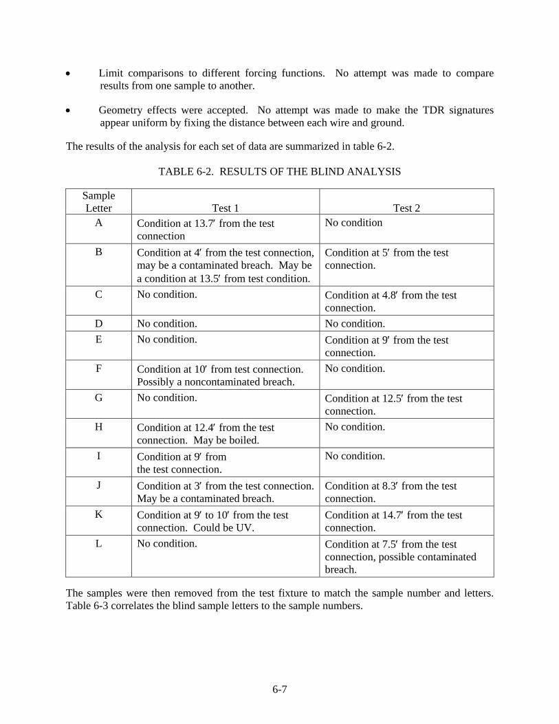
The results of the analysis for each set of data are summarized in table 6-2.

TABLE 6-2. RESULTS OF THE BLIND ANALYSIS

Sample Letter Test 1 Test 2

A Condition at 13.7′ from the test connection

No condition

B Condition at 4′ from the test connection, may be a contaminated breach. May be a condition at 13.5′ from test condition.

Condition at 5′ from the test connection.

C No condition. Condition at 4.8′ from the test connection.

D No condition. No condition. E No condition. Condition at 9′ from the test

connection. F Condition at 10′ from test connection.

Possibly a noncontaminated breach. No condition.

G No condition. Condition at 12.5′ from the test connection.

H Condition at 12.4′ from the test connection. May be boiled.

No condition.

I Condition at 9′ from the test connection.

No condition.

J Condition at 3′ from the test connection. May be a contaminated breach.

Condition at 8.3′ from the test connection.

K Condition at 9′ to 10′ from the test connection. Could be UV.

Condition at 14.7′ from the test connection.

L No condition. Condition at 7.5′ from the test connection, possible contaminated breach.

The samples were then removed from the test fixture to match the sample number and letters. Table 6-3 correlates the blind sample letters to the sample numbers.

6-7

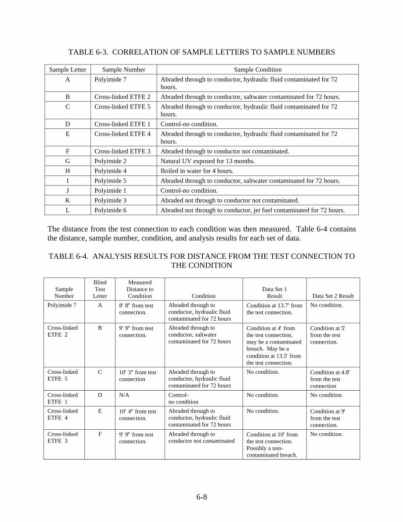
TABLE 6-3. CORRELATION OF SAMPLE LETTERS TO SAMPLE NUMBERS

Sample Letter Sample Number Sample Condition A Polyimide 7 Abraded through to conductor, hydraulic fluid contaminated for 72

hours. B Cross-linked ETFE 2 Abraded through to conductor, saltwater contaminated for 72 hours. C Cross-linked ETFE 5 Abraded through to conductor, hydraulic fluid contaminated for 72

hours. D Cross-linked ETFE 1 Control-no condition. E Cross-linked ETFE 4 Abraded through to conductor, hydraulic fluid contaminated for 72

hours. F Cross-linked ETFE 3 Abraded through to conductor not contaminated. G Polyimide 2 Natural UV exposed for 13 months. H Polyimide 4 Boiled in water for 4 hours. I Polyimide 5 Abraded through to conductor, saltwater contaminated for 72 hours. J Polyimide 1 Control-no condition. K Polyimide 3 Abraded not through to conductor not contaminated. L Polyimide 6 Abraded not through to conductor, jet fuel contaminated for 72 hours.

The distance from the test connection to each condition was then measured. Table 6-4 contains the distance, sample number, condition, and analysis results for each set of data. TABLE 6-4. ANALYSIS RESULTS FOR DISTANCE FROM THE TEST CONNECTION TO

THE CONDITION

Sample Number

Blind Test

Letter

Measured Distance to Condition Condition

Data Set 1 Result Data Set 2 Result

Polyimide 7 A 8′ 8″ from test connection.

Abraded through to conductor, hydraulic fluid contaminated for 72 hours

Condition at 13.7′ from the test connection.

No condition.

Cross-linked ETFE 2

B 9′ 9″ from test connection.

Abraded through to conductor, saltwater contaminated for 72 hours

Condition at 4′ from the test connection, may be a contaminated breach. May be a condition at 13.5′ from the test connection.

Condition at 5′ from the test connection.

Cross-linked ETFE 5

C 10′ 3″ from test connection

Abraded through to conductor, hydraulic fluid contaminated for 72 hours

No condition. Condition at 4.8′ from the test connection

Cross-linked ETFE 1

D N/A Control- no condition

No condition. No condition.

Cross-linked ETFE 4

E 10′ 4″ from test connection.

Abraded through to conductor, hydraulic fluid contaminated for 72 hours

No condition. Condition at 9′ from the test connection.

Cross-linked ETFE 3

F 9′ 9″ from test connection.

Abraded through to conductor not contaminated

Condition at 10′ from the test connection. Possibly a non-contaminated breach.

No condition.

6-8

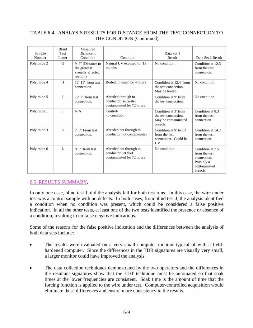
TABLE 6-4. ANALYSIS RESULTS FOR DISTANCE FROM THE TEST CONNECTION TO THE CONDITION (Continued)

Sample Number

Blind Test

Letter

Measured Distance to Condition Condition

Data Set 1 Result Data Set 2 Result

Polyimide 2 G 9′ 9″ (Distance to the greatest visually affected section)

Natural UV exposed for 13 months

No condition. Condition at 12.5′ from the test connection.

Polyimide 4 H 12′ 11″ from test connection.

Boiled in water for 4 hours Condition at 12.4′ from the test connection. May be boiled.

No condition.

Polyimide 5 I 12′ 7″ from test connection.

Abraded through to conductor, saltwater contaminated for 72 hours

Condition at 9′ from the test connection.

No condition.

Polyimide 1 J N/A Control- no condition

Condition at 3′ from the test connection. May be contaminated breach.

Condition at 8.3′ from the test connection

Polyimide 3 K 7′ 6″ From test connection.

Abraded not through to conductor not contaminated

Condition at 9′ to 10′ from the test connection. Could be UV.

Condition at 14.7′ from the test connection.

Polyimide 6 L 8′ 8″ from test connection.

Abraded not through to conductor, jet fuel contaminated for 72 hours

No condition. Condition at 7.5′ from the test connection. Possibly a contaminated breach.

6.5 RESULTS SUMMARY.

In only one case, blind test J, did the analysis fail for both test runs. In this case, the wire under test was a control sample with no defects. In both cases, from blind test J, the analysis identified a condition when no condition was present, which could be considered a false positive indication. In all the other tests, at least one of the two tests identified the presence or absence of a condition, resulting in no false negative indications. Some of the reasons for the false positive indication and the differences between the analysis of both data sets include: • The results were evaluated on a very small computer monitor typical of with a field-

hardened computer. Since the differences in the TDR signatures are visually very small, a larger monitor could have improved the analysis.

• The data collection techniques demonstrated by the two operators and the differences in

the resultant signatures show that the EDT technique must be automated so that soak times at the lower frequencies are consistent. Soak time is the amount of time that the forcing function is applied to the wire under test. Computer-controlled acquisition would eliminate these differences and ensure more consistency in the results.

6-9

• As mentioned earlier, the wires were loosely installed in the EMT and no attempt was made to create a uniform distance between each wire and ground. If the wire samples attached to the outside conduit to simulate a typical installation in an aircraft were placed in a bundle, the analysis may have been more accurate. If each wire had a more uniform geometry, the TDR signatures may have been flatter, making subtle impedance changes more easily detected.

6.6 SUPPLEMENTAL TESTS AND ANALYSIS.

Two supplemental tests, requested by FAA personnel, were performed during the verification at the FAA William J. Hughes Technical Center. The first supplemental test configuration consisted of electrically connecting all the wire samples together, except one wire. The EDT was performed between the single wire and the other wires in the bundle. The single wire was validation sample L, polyimide sample 6, which was abraded not through to the conductor, and jet fuel contaminated for 72 hours. The jet fuel contaminated abrasion was located 8 feet 8 inches from the test connection. Figure 6-12 shows a 64x magnification of an area of possible degradation located 12.2 feet from the test connection. Figure 6-12 is a comparison of four TDR signatures acquired with a 5 volt, sine wave forcing function at frequencies of 20 MHz (green trace), 200 MHz (cyan trace), 2 Hz (magenta trace), and 20 Hz (red trace).

Area of Increased Impedance

Located at 12.2 feet

FIGURE 6-12. RESULTS FROM SUPPLEMENTAL TEST 1

6-10

The second supplemental test requested by FAA personnel consisted of testing one wire sample with the other wires electrically connected together outside the EMT. The wire bundle was taped to the outside of the test fixture to maintain the geometry. Figure 6-3 is a comparison of TDR signatures acquired for this configuration. This figure is a comparison of four TDR signatures acquired with a 5 volt, sine wave forcing function at frequencies of 20 MHz (green trace), 200 MHz (cyan trace), 2 Hz (magenta trace), and 20 Hz (red trace). The section of possible degradation was at the same approximate distance from the test point as determined from the previous test, 12.2 feet for the first supplemental test, and 13.6 feet for the second supplemental test. This difference may be due to geometry effects and a difference in Vp.

Slight Separation of TDR Signatures

Located at 13.6 feet

FIGURE 6-13. RESULTS FROM SUPPLEMENTAL TEST 2

6-11/6-12

7. CONCLUSIONS AND RECOMMENDATIONS.

The primary goal of this research effort was to demonstrate and validate the underlying theory of the new excited dielectric test (EDT) test method developed by CM Technologies. Overall, the results demonstrated how the EDT test method detected and located known wiring defects under controlled test conditions. The EDT found common defects that may be present in aircraft wiring systems, including abrasions, fluid contamination, and thermal degradation. At its core, the new EDT method stimulates the wire under test to reveal a greater sensitivity to defect detection and location than traditional time domain reflectometry (TDR) test methods. Further, application of the EDT technique currently uses a qualitative comparison methodology to identify localized areas of insulation degradation; these appear as readily discernable differences in the resulting TDR signatures. This unique feature provides technicians with a valuable tool to characterize localized insulation conditions without the need for historical baseline data; i.e., implementation of the EDT test methodology generates a comparative data set using global insulation quality as a reference against which localized qualities are evaluated. The response of various defects and various materials to the EDT method is a strongly related to the frequency of the forcing function applied during the test. Laboratory data developed during this effort shows that this response is repeatable and predictable for the narrow set of materials and defects studied. Based on these results, other polar insulation materials are likely to exhibit similar responses to the EDT method. The research demonstrated that the EDT method represents a fundamentally sound approach to defect detection and location. However, there were small defects that went undetected during the development and validation effort. Based upon prior experience with traditional TDR and other test methods, it is believed that the threshold for detection for these small defects will be lowered substantially when applied to installed aircraft wiring due to the presence of moisture, dust, lubricants, and other contaminates.

7-1/7-2

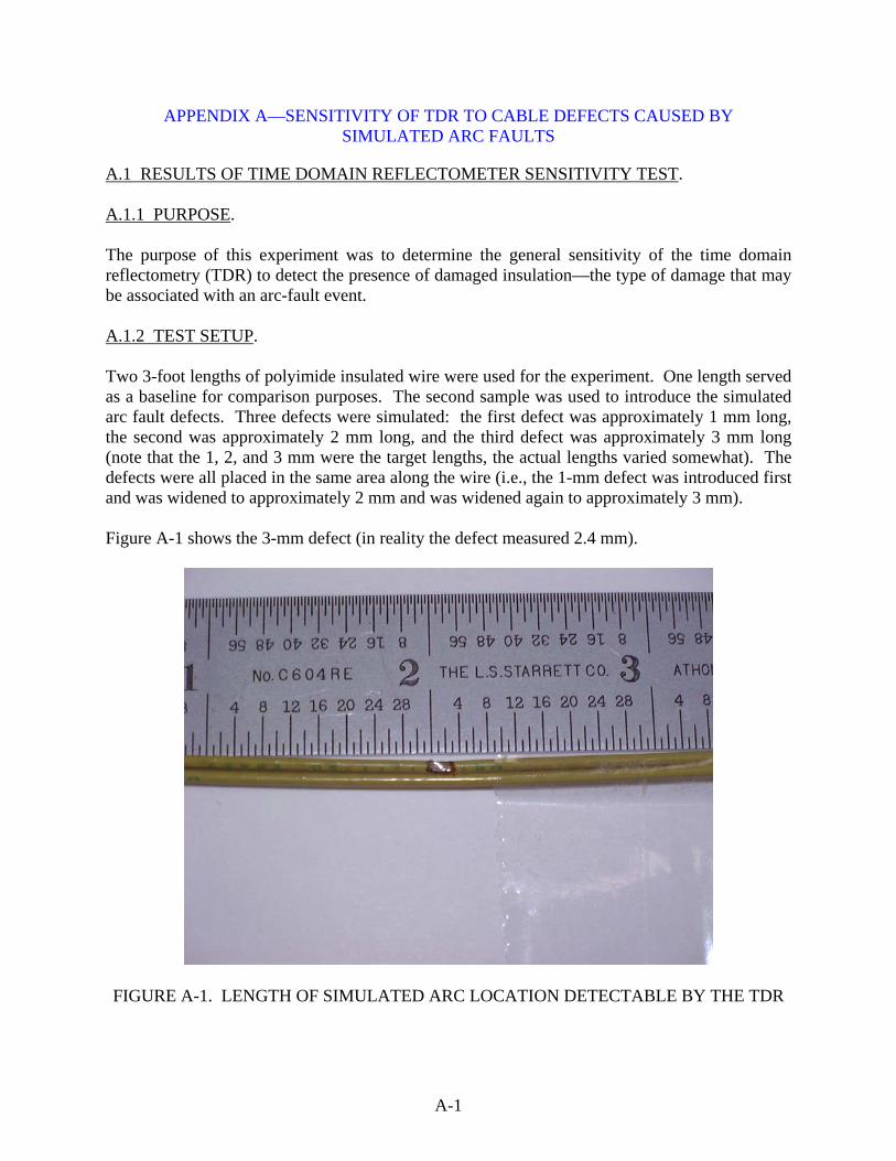
APPENDIX A—SENSITIVITY OF TDR TO CABLE DEFECTS CAUSED BY SIMULATED ARC FAULTS

A.1 RESULTS OF TIME DOMAIN REFLECTOMETER SENSITIVITY TEST. A.1.1 PURPOSE. The purpose of this experiment was to determine the general sensitivity of the time domain reflectometry (TDR) to detect the presence of damaged insulation—the type of damage that may be associated with an arc-fault event. A.1.2 TEST SETUP. Two 3-foot lengths of polyimide insulated wire were used for the experiment. One length served as a baseline for comparison purposes. The second sample was used to introduce the simulated arc fault defects. Three defects were simulated: the first defect was approximately 1 mm long, the second was approximately 2 mm long, and the third defect was approximately 3 mm long (note that the 1, 2, and 3 mm were the target lengths, the actual lengths varied somewhat). The defects were all placed in the same area along the wire (i.e., the 1-mm defect was introduced first and was widened to approximately 2 mm and was widened again to approximately 3 mm). Figure A-1 shows the 3-mm defect (in reality the defect measured 2.4 mm).

FIGURE A-1. LENGTH OF SIMULATED ARC LOCATION DETECTABLE BY THE TDR

A-1

Figure A-2 shows a side view of the 3-mm defect. Notice the insulation was only removed from one-half of the circumference to more realistically simulate an arcing event.

Side View of Simulated Arc Fault Defect

FIGURE A-2. SIDE VIEW OF THE SIMULATED ARC-FAULT DEFECT

A.1.3 RESULTS. Since all the simulated defects were clean (i.e., no contamination), the expected response of the TDR to a simulated arc-fault defect was an increase in impedance (Z), where

Impedance (Z) = SQRT(L/C) and

Capacitance = (εA)/d where ε = 2.0 to 3.0 for polyimide insulation and ε = 1.0 for air (or the absence of insulation). In the local area near the defect, the incremental capacitance would decrease because of the polyimide insulation being replaced by air. This decrease in capacitance would produce a corresponding increase in impedance. The 1-mm defect was not visible to the TDR. There was essentially no difference between the two signatures. The 2-mm defect did affect the TDR signature, but only very slightly.

A-2

The signatures from the 3-mm defect, shown in figure A-3, produced a discernable separation.

Turquoise signature indicates an area of

decreased capacitance near the 2.4 mm defect

Yellow Signature is the baseline (i.e., no

faults)

FIGURE A-3. TME DOMAIN REFLECTOMETRY SIGNATURES FROM BASELINE AND

2.4-mm DEFECT WIRE SAMPLES

A.2 CONCLUSIONS. • Based on the results from this experiment, the length of detectable defects, with no

contamination, is between 2 and 3 mm. • If any residue or contamination occurs as the result of an actual arcing event, the time

domain reflectometry (TDR) may become more sensitive to shorter defect lengths. Carbon residues would result in a larger capacitance change.

• In a nonlaboratory environment, baseline data would be required. Comparison of TDR

signatures between similar circuits or geometries on the aircraft would be of limited use in detecting these subtle types of defects.

A-3/A-4