The design of an optimal retrospective rating

plan

Xinxiang Chen∗

School of Mathematical Sciences, Xiamen University, Xiamen 361005, China

Yichun Chi†

China Institute for Actuarial Science

Central University of Finance and Economics, Beijing 100081, China

Ken Seng Tan‡

Department of Statistics and Actuarial Science, University of Waterloo

Waterloo, Ontario N2L 3G1, Canada

Abstract

A retrospective rating plan, whose insurance premium depends upon an insured’s

actual loss during the policy period, is a special insurance agreement widely used

in liability insurance. In this paper, the design of an optimal retrospective rating

plan is analyzed from the perspective of the insured who seeks to minimize its risk

exposure in the sense of convex order. In order to reduce the moral hazard, we

assume that both the insured and the insurer are obligated to pay more for a larger

realization of the loss. Under the further assumptions that the minimum premium is

zero, the maximum premium is proportional to the expected indemnity, and the basic

premium is the only free parameter in the formula for retrospective premium given

by Meyers (2004) and that the basic premium is determined in such a way that the

expected retrospective premium equates to the expected indemnity with a positive

safety loading, we formally establish the relationship that the insured will suffer more

risk for a larger loss conversion factor or a higher maximum premium. These findings

suggest that the insured prefers an insurance policy with the expected value premium

principle, which is a special retrospective premium principle with zero loss conversion

factor. In addition, we show that any admissible retrospective rating plan is dominated

∗E-mail address: xxchen@xmu.edu.cn(Xinxiang Chen)†Corresponding author. E-mail address: yichun 1982@hotmail.com(Yichun Chi)‡E-mail address: kstan@uwaterloo.ca(Ken Seng Tan)

1

by a stop-loss insurance policy. Finally, the optimal retention of a stop-loss insurance

is derived numerically under the criterion of minimizing the risk-adjusted value of the

insured’s liability where the liability valuation is carried out using the cost-of-capital

approach based on the conditional value at risk.

Key-words: Conditional value at risk; Convex order; Moral hazard; Optimal retrospective

rating plan; Stop-loss insurance.

1 Introduction

Insurance has become an indispensable tool for an individual or a corporation to manage its risk.

An income earner who wishes to protect his/her surviving family’s income in the event of his/her

death can achieve the aim by purchasing a life insurance policy. Similarly, car insurance can be

used to recover some of the losses incurred to the driver in the event of a car accident. Other

insurance policies such as unemployment insurance, health and dental insurance, and product

liability, are typically available to a corporation to provide some form of protection to its employees

and the corporation itself.

By transferring all or part of its risk to an insurance company (i.e. the insurer), the individual

or the corporation (i.e. the insured) incurs an additional cost in the form of the insurance

premium. The insurance premium is expected to increase with higher expected risk that is ceded

to the insurer. This implies that the insured can transfer more of its risk to an insurer at the

expense of a higher insurance premium. If the insured were to reduce the cost of insurance, his

risk exposure will be much higher. This classical tradeoff implies that there exists an optimal

strategy between risk retaining and risk transferring. By formulating as an optimization problem

with an appropriate objective and constraints, this allows the insured to optimally determine the

best strategy to insure its risk.

The pioneering work on optimal insurance is attributed to Borch (1960) who shows that the

stop-loss insurance is optimal under the criterion of minimizing the variance of the insured’s

retained risk when the insurance premium is calculated by the expected premium principle. By

maximizing the expected utility of the final wealth of a risk-averse insured, Arrow (1963) derives

a similar result justifying the optimality of stop-loss insurance. These classical results have been

extended in a number of interesting directions. One generalization is to consider more complicated

premium principles, as opposed to the standard expected premium principle. These results can

be found in Raviv (1979), Young (1999), Kaluszka (2001), Gajek and Zagrodny (2004), Kaluszka

and Okolewski (2008), Bernard and Tian (2009), and references therein. Due to the popularity of

risk measures such as value at risk(VaR) and conditional value at risk(CVaR) in quantifying the

financial and insurance risks, the risk measure based optimal insurance/reinsurance problems have

been studied by many researchers in the past ten years. See, for example, Cai and Tan (2007),

Cai et al. (2008), Balbas et al. (2009), Cheung (2010), Chi and Tan (2011), Chi (2012), Asimit et

al. (2013), Cong and Tan (2014), and references therein. In the afore-mentioned studies, most of

the optimization criteria have a common property of preserving the convex order, which enables

2

us to use a unified approach to tackle optimal insurance problems. For unified treatments of the

problems, we refer to Van Heerwaarden et al. (1989), Gollier and Schlesinger (1996) and Chi and

Lin (2014) .

The existing literature typically assumes that the insurance premium is known at the inception

of the insurance contract and is calculated based on the distribution of indemnity about which

the insured and the insurer have symmetric information. However, in some insurance practice,

not only the indemnity distribution but also its actual realization are sometimes used to compute

the insurance premium. A special example is the retrospective rating plan which is widely used in

liability insurance and is summarized in Meyers (2004). More precisely, let π(.) denote a premium

principle of a retrospective rating plan, then for any nonnegative risk Y ,

π(Y ) = min max (B(Y ) + L(Y )× Y )T, G(Y ) , H(Y ) , (1.1)

where B(Y ) ≥ 0 is the basic premium, L(Y ) ≥ 0 is the loss conversion factor and covers the

loss adjustment expenses, T > 1 is the tax multiplier including premium tax, and G(Y ) ≥ 0 and

H(Y ) ≥ 0 represent the minimum premium and maximum premium, respectively. Compared

to other well-known premium principles such as the expected value premium principle and the

standard deviation premium principle, the retrospective rating plan based premium principle

(1.1) is considerably more complicated. First, it requires five parameters in order to fully specify

the above premium principle. Second, while the parameters B,L,G,H depend explicitly on

the nonnegative risk Y as indicated in (1.1), in practice some of these parameters could be

related to Y implicitly. For example, as discussed in Meyers (2004) that in practice four of the

parameters are agreed upon between the insured and the insurer at the inception of the insurance

agreement. Typically these are some deterministic constants. Once these four parameters are

well-specified, the remaining “free” fifth parameter is then determined by a desired expected

retrospective premium. In this case, the fifth parameter depends explicitly on Y . The parameter

L(Y ) or B(Y ) is often set to be the free parameter. Consequently, all these five parameters

have deterministic values when the insurance contract is in effect. Another distinctive feature

of the above retrospective rating plan is that the resulting insurance premium depends on the

insured’s actual loss. This implies that the actual insurance premium is not known until the

insurance policy has matured. This feature is also well suited for the above mentioned optimal

insurance/reinsurance models since the underlying problems are typically formulated as one-

period optimization problems. For these reasons, it is very interesting to develop the optimal

strategy for the above retrospective rating plan. However, to the best of our knowledge, there is

hardly any paper that studies its optimality.

In this paper, the design of an optimal retrospective rating plan is studied from the perspective

of an insured who seeks to minimize its risk exposure in the sense of convex order, where the

insurance premium is calculated by a retrospective premium principle (1.1). For simplicity, the

minimum premium and the maximum premium are assumed to be

G(Y ) = 0 and H(Y ) = (1 + ϑ)E[Y ] (1.2)

for some loading coefficient ϑ > 0. Moreover, we assume that the basic premium B(Y ) is the

3

only free parameter which is the minimal solution to the following equation

E[π(Y )] = (1 + ρ)E[Y ], (1.3)

where ρ ∈ (0, ϑ) is the safety loading coefficient. In order to reduce the moral hazard, we further

assume that both the insured and the insurer are obligated to pay more for a larger realization

of loss. The design of an optimal retrospective rating plan is analyzed from two aspects. On one

hand, we analyze the effects of the changes in the parameters of retrospective premium principle

on the insured’s risk exposure. More specifically, by a comparative static analysis, we find that the

insured will suffer more risk for a larger loss conversion factor or a higher ϑ. These findings suggest

that the insured will prefer an insurance contract with the expected value principle which is a

special retrospective premium principle with zero loss conversion factor. On the other hand, by

fixing the retrospective premium principle we discuss the optimal ceded strategies. More precisely,

we show, via a constructive approach, any admissible retrospective rating plan is dominated by

a stop-loss insurance contract. Noting that the expected value premium principle is a special

case, our result generalizes Theorem 6.1 of Van Heerwaarden et al. (1989). Finally, to illustrate

the applicability of our results, we derive numerically the optimal retention of stop-loss insurance

under the criterion of minimizing the risk-adjusted value of the insured’s liability where the

liability valuation is carried out using a cost-of-capital approach based on CVaR, and analyze the

effects of loss conversion rate and the loading coefficient ϑ on the optimal retentnion.

The rest of this paper is organized as follows. In Section 2, we describe a retrospective rating

plan. Under such a plan, the effects of loss conversion factor and the loading coefficient in the

maximum premium on the insured’s total risk exposure are analyzed in Section 3. Section 4

shows that any admissible insurance policy is dominated by a stop-loss insurance contract. To

illustrate the applicability of the results established in Section 4, we derive the optimal retention

of stop-loss insurance under the criterion of minimizing the risk-adjusted value of an insured’s

liability in Section 5. Finally, some concluding remarks are provided in Section 6.

2 A retrospective rating plan

Suppose X denotes the amount of loss an insured is facing over a given time period. We assume

X is a non-negative random variable defined on a probability space (Ω,F ,P) with cumulative dis-

tribution function (cdf) FX(x) = P(X ≤ x), x ≥ 0 and 0 < E[X] <∞. An optimal retrospective

rating plan is concerned with an optimal partition of X into two parts: f(X) and Rf (X), where

f(X), satisfying 0 ≤ f(X) ≤ X, represents the portion of the loss that is ceded to an insurer,

while Rf (X) = X − f(X) represents the retained loss by the insured. The functions f(x) and

Rf (x) are known as the ceded and retained loss functions, respectively. As pointed out earlier,

we assume both the insured and the insurer are obligated to pay more for a larger realization

of loss in order to reduce the moral hazard. In other words, both the ceded loss function f(x)

and the retained loss function Rf (x) should be increasing. As shown in Chi and Tan (2011), it is

equivalent to that the ceded loss function is increasing and Lipschitz continuous, i.e.

0 ≤ f(x2)− f(x1) ≤ x2 − x1, ∀ 0 ≤ x1 ≤ x2. (2.1)

4

Thus, the set of admissible ceded loss functions is given by

C , 0 ≤ f(x) ≤ x : both f(x) andRf (x) are increasing functions . (2.2)

Under a retrospective rating plan, the insurance premium is calculated according to (1.1). For

the sake of simplicity, we make the following assumptions:

Assumption 2.1. (1) The maximum premium H(Y ) and the minimum premium G(Y ) are set

as in (1.2); (2) the basic premium B(Y ) is the only free parameter determined by (1.3).

Under the above assumption, the loss conversion factor L(Y ) is now independent of Y , and

we rewrite it by L for brevity. As a consequence, the retrospective premium principle π(.) can

be rewritten by

π(Y ) = min (B(Y ) + L× Y )T, (1 + ϑ)E[Y ] (2.3)

for any non-negative random variable Y . It is easy to see from the above equation and (1.3) that

(1 + ϑ)E[Y ] > B(Y )× T if and only if E[Y ] > 0. (2.4)

In particular, when L = 0, it follows from the above equation that

π(Y ) = (1 + ρ)E[Y ], (2.5)

which is exactly the expected value principle. Moreover, both (1.3) and (2.3) ensure the free

parameter B(Y ) can be easily derived from the following equation

(ϑ− ρ)E[Y ] = E[((1 + ϑ)E[Y ]− (B(Y ) + LY )T )+

], (2.6)

where (x)+ = max(x, 0).

In the presence of a retrospective rating plan f(x), the risk the insured is facing is no longer

X; it is the total risk exposure Tf (X) which is defined as

Tf (X) = Rf (X) + π(f(X)). (2.7)

Recall that the insurance premium depends on the actual loss. Thus, in order to mitigate the

moral hazard, we should assume T′

f (x) ≤ 1, a.s. for any f ∈ C, which is equivalent to

TL ≤ 1. (2.8)

To quantify the insured’s total risk exposure Tf (X), a number of risk measures, including

those that are coherent and convex, can be used. For a detailed discussion of risk measures, see

Artzner et al. (1999) and Follmer and Schied (2004). Due to the prevalent use of the convex

order for risk ranking in finance and insurance, most risk measures, including the CVaR, have a

common property of convex order preserving. To ensure that our results are as general as possible

so that our results are applicable to a wide range of insured’s risk preferences, in this paper we

only assume that the adopted risk measure preserves the convex order. Specifically, let Ψ(·), a

5

mapping from the set of non-negative random variables to R, be the risk measure the insured

uses, then

Ψ(Y ) ≤ Ψ(Z), if Y ≤cx Z.1

Note that Tf (X) depends on the retrospective premium principle π(.) and the ceded loss function

f(x). We will analyze the effects of these two factors on the insured’s risk measure Ψ(Tf (X)) in

the next two sections respectively.

3 The effects of retrospective premium principle

Recall that the retrospective premium principle defined in this paper has four non-free parameters,

namely the loss conversion factor L, the loading coefficient ϑ for the maximum premium, the

loading coefficient ρ in (1.3) and the tax multiplier T . In this section, we will study the effects

of these parameters on the insured’s risk exposure Tf (X). In particular, we will only focus on L

and ϑ, since the tax rate is usually set by the government and is beyond our control and we also

fix ρ such that the expected retrospective premium is a constant. The main result of this section

is obtained in the following theorem.

Theorem 3.1. Under Assumption 2.1, given a ceded strategy f(x) ∈ C, the insured’s total risk

exposure Tf (X) is increasing in the loss conversion factor L and the loading coefficient ϑ in the

sense of convex order.

Proof. As Tf (X) is a function of the loss conversion factor L, we rewrite Tf (X) by Tf (X;L) to

emphasize this dependence. We first show that

Tf (X;L1) ≤cx Tf (X;L2), ∀0 ≤ L1 < L2 ≤1

T. (3.1)

Specifically, we rewrite the basic premium by Bif for Li, then it follows from (1.3) and (2.3) that

Tf (X;Li) = Rf (X) + (1 + ϑ)E[f(X)]− ψi(X), i = 1, 2, (3.2)

where

ψi(x) ,((1 + ϑ)E[f(X)]−BifT − LiTf(x)

)+, x ≥ 0.

The following proof is divided into two cases: E[f(X)] = 0 and E[f(X)] > 0.

• If E[f(X)] = 0, we have f(X) = 0, a.s. and ψi(x) = 0 for i = 1, 2, then the above equation

implies Tf (X;Li) = X, a.s.. Thus, the result is obtained.

• Otherwise, if E[f(X)] > 0, it follows from (2.6) that

E[ψi(X)] = (ϑ− ρ)E[f(X)], (3.3)

1Here, Y ≤cx Z is equivalent to

E[Y ] = E[Z] and E[(Y − d)+] ≤ E[(Z − d)+], ∀d ∈ R (2.9)

provided that the expectations exist. See Shaked and Shanthikumar (2007) for more details on the theory of

stochastic orders.

6

then we have B1f ≥ B2

f . By defining

xi , sup x ≥ 0 : ψi(x) > 0 , i = 1, 2, (3.4)

it follows from (2.1) and (2.4) that xi > 0. Moreover, we must have x2 ≤ x1; otherwise, if

x2 > x1, we have

ψ2(x)− ψ1(x) =

(B1

f −B2f )T + (L1 − L2)Tf(x), x ∈ [0, x1];

ψ2(x) > 0, x ∈ (x1, x2);

0, x ≥ x2.

From the above equation, it is easy to see that ψ2(x)− ψ1(x) is decreasing and continuous

over [0, x1], then it is positive over [0, x2) and is equal to zero for x ≥ x2. Since it is assumed

that E[f(X)] > 0, then using (3.3) and (3.4), we must have E[ψ2(X)] > E[ψ1(X)], which

contradicts (3.3).

Now, using the similar arguments, it is easy to see that over [0, x2], ψ2(x) − ψ1(x) is a

decreasing continuous function with ψ2(0) − ψ1(0) = (B1f − B2

f )T ≥ 0. Moreover, for any

x > x2, we have ψ2(x) − ψ1(x) = −ψ1(x) which is a non-positive increasing function. As

a consequence, we get that ψ1(x) up-crosses ψ2(x).2 Using Lemma 3 in Ohlin (1969) and

(3.3), we get

(1 + ϑ)E[f(X)]− ψ1(X) ≤cx (1 + ϑ)E[f(X)]− ψ2(X).

Moreover, it is easy to see from (2.1) that the retained loss function Rf (x) is comonotonic

with (1 + ϑ)E[f(X)]− ψi(x), then (3.1) can be obtained by using Corollary 1 in Dhaene et

al. (2002).

Next, we similarly rewrite Tf (X) by Tϑf (X) andB(f(X)) byBϑf to emphasize their dependence

on the loading coefficient ϑ. We demonstrate that

Tϑ1

f (X) ≤cx Tϑ2

f (X), ∀ρ < ϑ1 < ϑ2.

More specifically, if E[f(X)] = 0, the similar analysis leads to Tϑif (X) = X, a.s. so that the above

equation holds. Otherwise, if E[f(X)] > 0, as in (3.2), we have

Tϑif (X) = Rf (X) + φi(X), i = 1, 2,

where

φi(x) , minBϑif T + LTf(x), (1 + ϑi)E[f(X)]

, x ≥ 0.

The definition of φi(x) together with (1.3) implies Bϑ1

f ≥ Bϑ2

f and

E[φi(X)] = (1 + ρ)E[f(X)], i = 1, 2.

2A function g(x) is said to up-cross a function h(x), if there exists an x0 ∈ R such thatg(x) ≤ h(x), x < x0;

g(x) ≥ h(x), x > x0.

7

By defining

xi , sup

x ≥ 0 : f(x) ≤

(1 + ϑi)E[f(X)]−Bϑif TLT

,

we obviously have 0 < x1 ≤ x2 and

φ1(x)− φ2(x) =

(Bϑ1

f −Bϑ2

f )T ≥ 0, 0 ≤ x ≤ x1;

(1 + ϑ1)E[f(X)]−Bϑ2

f T − LTf(x) is decreasing, x1 < x ≤ x2;

(ϑ1 − ϑ2)E[f(X)] < 0, x > x2.

Thus, φ2(x) up-crosses φ1(x). Using Lemma 3 in Ohlin (1969), we have φ1(X) ≤cx φ2(X).

Moreover, it follows from (2.1) that Rf (x) and φi(x) are comonotomic, then using Corollary 1 in

Dhaene et al. (2002) again, we get the final result. The proof is thus complete.

From the above theorem, we know that the insured who buys a retrospective rating plan pays

less basic premium but suffers more risk for the premium principle with larger loss conversion

factor or the larger loading coefficient for maximum premium in the sense of convex order. As

a result, a prudent risk-averse insured will choose a retrospective rating plan with the premium

principle including smaller loss conversion factor or lower loading coefficient. In the extreme case

the insured will prefer the insurance contract with expected value premium principle as it is a

special retrospective premium principle with zero loss conversion factor. Moreover, these findings

are available for all the insureds whose risk preferences preserve the convex order. In the next

section, we will fix the retrospective premium principle and study an optimal ceded strategy.

4 An optimal ceded strategy

In this section, we will investigate optimal retrospective rating plans for an insured under a

retrospective premium principle. More specifically, we attempt to solve the following optimal

insurance problem:

minf∈C

Ψ(Tf (X)). (4.1)

Recall that the basic premium B(f(X)) is an implicit functional of the ceded loss f(X). It

becomes very challenging to solve the above infinite-dimensional minimization problem. However,

using a constructive approach, we obtain the main result of this section in the following theorem.

Theorem 4.1. Under the retrospective premium principle π(.) in (2.3), any admissible insurance

contract is dominated by a stop-loss insurance policy. More specifically, for any f ∈ C, there exists

a stop-loss insurance fd(x) = (x− d)+ for some d ≥ 0 such that

E[fd(X)] = E[f(X)] and Tfd(X) ≤cx Tf (X). (4.2)

As a result, the optimal insurance model (4.1) is equivalent to

mind≥0

Ψ(Tfd(X)). (4.3)

8

Proof. For any f ∈ C, if E[f(X)] = 0, we have f(X) = 0, a.s. and hence Tf (X) = X, a.s., then

the result is trivial. Thus, we assume E[f(X)] > 0. To proceed, we define

xf , supx ≥ 0 : f(x) ≤ ((1 + ϑ)E[f(X)]/T −Bf ) /L

, (4.4)

where Bf is an abbreviation of B(f(X)). It is easy to see from (2.4) that xf > 0.

We now show that f(x) is dominated by a two-layer insurance policy, and the proof is divided

into two cases: xf =∞ and xf <∞.

(i) For the case xf =∞, we denote

w(t) , E[L(t,t+((1+ϑ)E[f(X)]/T−Bf )/L](X)], ∀t ≥ 0,

where L(a,b](Y ) represents a layer (a, b] of a non-negative risk Y and is formally defined as

L(a,b](Y ) , min (Y − a)+, b− a , 0 ≤ a ≤ b.

It is easy to see that w(t) is a decreasing continuous function with w(∞) = 0. Moreover,

we have

w(0) = E [minX, ((1 + ϑ)E[f(X)]/T −Bf ) /L]

≥ E [minf(X), ((1 + ϑ)E[f(X)]/T −Bf ) /L] = E[f(X)],

where the last equality is derived by (4.4) and the assumption of xf = ∞. Consequently,

there must exist a t0 ∈ [0,∞) such that w(t0) = E[f(X)].

Further, since it is assumed that xf =∞, we have

π(f(X)) = T × (Bf + L× f(X)),

then it follows from (1.3) that

Bf × T = (1 + ρ− LT )E[f(X)],

which in turn implies

Tf (X) = LTX + (1− LT )Rf (X) + (1 + ρ− LT )E[f(X)].

Now, we introduce a layer insurance policy with ceded loss function

f(x) , L(t0,t0+((1+ϑ)E[f(X)]/T−Bf )/L](x), x ≥ 0. (4.5)

Then we have

E[f(X)] = w(t0) = E[f(X)].

Furthermore, it follows from (2.6) that

(ϑ− ρ)

LTw(t0) = E

[((1 + ϑ)w(t0)−BfT )/TL− f(X)

)+

]= ((1 + ϑ)w(t0)−BfT )/TL−

∫ ((1+ϑ)w(t0)−BfT )/TL

0

Sf(X)(x)dx(4.6)

9

where SY (t) = 1− FY (t) is the survival function of random variable Y . Similarly, we have

ϑ− ρLT

w(t0) = ((1 + ϑ)w(t0)−BfT ) /TL−∫ ((1+ϑ)w(t0)−BfT )/TL

0

Sf(X)(x)dx

= ((1 + ϑ)w(t0)−BfT ) /TL− w(t0)

= ((1 + ϑ)w(t0)−BfT )/TL−∫ ((1+ϑ)w(t0)−BfT )/TL

0

Sf(X)(x)dx,

where the second equality follows from the assumption xf = ∞ and the last equality is

derived by the fact f(x) ≤ ((1 + ϑ)w(t0) − BfT )/TL for any x ≥ 0. By comparing the

above equation with (4.6), since it is assumed that E[f(X)] > 0, then it is easy to get

Bf = Bf ,

which in turn implies xf =∞. As a result, we have

Tf (X) = LTX + (1− LT )Rf (X) + (1 + ρ− LT )w(t0).

From (2.1) and (2.8), we know that the retained loss function is increasing and Lipschitz

continuous, then it is easy to show that the function LTx + (1 − LT )Rf (x) up-crosses

LTx + (1 − LT )Rf (x). Further, note that E[Tf (X)] = E[Tf (X)], then it follows from

Lemma 3 in Ohlin (1969) that Tf (X) ≤cx Tf (X).

(ii) Now, we consider the case 0 < xf <∞. Building upon f , we define

f1(x) ,

f(x), 0 ≤ x ≤ xf ;

f(xf ) + (x− df )+, x > xf ,

where df ≥ xf is determined by E[f1(X)] = E[f(X)]. Using (2.6), we obtain

(ϑ− ρ)E[f(X)] = E[((1 + ϑ)E[f(X)]− (Bf + Lf(X))T ) 1X≤xf

]= E

[((1 + ϑ)E[f1(X)]− (Bf + Lf1(X))T )+

],

where 1A is an indicator function of the event A. By comparing the above equation with

(2.6) for Y = f1(X), it is easy to get

Bf1 = Bf . (4.7)

Moreover, according to the definition of Tf (X), we have

Tf (x) =

BfT + x− (1− LT )f(x), 0 ≤ x ≤ xf ;

Rf (x) + (1 + ϑ)E[f(X)], x > xf .(4.8)

By (2.1) and (4.7), it is easy to see that Tf (x) up-crosses Tf1(x). Moreover, we can get from

(1.3) that

E[Tf (X)] = E[Rf (X)] + E[π(f(X))] = E[X] + ρE[f(X)] = E[Tf1(X)]. (4.9)

10

Consequently, using Lemma 3 in Ohlin (1969) again, we get

Tf1(X) ≤cx Tf (X).

Further, building upon f1, it follows from (2.1) that there must exist an a satisfying 0 ≤a ≤ xf − f(xf ) such that E[f1(X)] = E[f2(X)], where f2(x) is a ceded loss function defined

as

f2(x) = L(a,a+f(xf )](x) + (x− df )+, x ≥ 0.

Using (2.1) again, it is easy to verify that f2(x) up-crosses f1(x), then it follows from Lemma

3 in Ohlin (1969) that f1(X) ≤cx f2(X), which together with (2.6) implies

Bf1 ≤ Bf2 .

If Bf1 = Bf2 , let

f(x) = f2(x), x ≥ 0, (4.10)

then we have xf = xf1 = xf2 = df and f(xf ) = f(xf ). For this case, it is easy to see from

(4.8) that Tf1(x) up-crosses Tf (x). Moreover, (4.9) implies E[Tfi(X)] = E[X] + ρE[f(X)]

for i = 1, 2, then it follows from Lemma 3 in Ohlin (1969) that

Tf (X) ≤cx Tf1(X) ≤cx Tf (X).

Otherwise, if Bf1 < Bf2 , then f2(xf2) < f(xf ) such that

a < xf2 ≤ a+ f(xf ) < xf ≤ df = xf1 .

For any 0 ≤ x ≤ a, we have f2(x) = 0, then it follows from the Lipschitz-continuous

property of f1(x) and (4.8) that

Tf1(x)− Tf2(x) ≤ 0.

For any x ∈ (a, a+ f(xf )], (4.8) implies T′

f2(x) = 0 orLT but T

′

f1(x) ≥ LT . Thus, over this

interval, Tf1(x)− Tf2(x) is increasing. Over the interval (a+ f(xf ), df ], we have

Tf1(x)− Tf2(x) = Bf1T − (1 + ϑ)E[f(X)] + f(xf )− (1− LT )f1(x),

which is decreasing in x and is equal to 0 when x = df . Moreover, it is easy to see from

(4.8) that Tf1(x)− Tf2(x) = 0 for any x > df . Collecting the above arguments yields that

Tf1(x) up-crosses Tf2(x). Thus, Lemma 3 in Ohlin (1969) again leads to

Tf2(X) ≤cx Tf1(X).

Similar to the construction of f1 from f and based on f2, we can construct a ceded loss

function of the form

f(x) = L(a,a+f2(xf2 )](x) + (x− df2)+ (4.11)

for some xf2 ≤ df2 ≤ df such that

E[f2(X)] = E[f(X)], xf = df2 , f(xf ) = f2(xf2) and Tf (X) ≤cx Tf2(X) ≤cx Tf (X).

11

In summary, any admissible insurance contract f(x) is dominated by a layer insurance policy

f(x) or a two-layer insurance policy f(x). Moreover, from (4.5), (4.10) and (4.11), we find that

f(x) and f(x) have the similar structure and can be written in a unified form as

h(x) = L(a,a+((1+ϑ)E[h(X)]−BhT )/TL](x) + (x− xh)+.

Furthermore, for any ceded loss function h with the above structure, there must exist a stop-loss

insurance policy fd(x) with a ≤ d ≤ xh − ((1 + ϑ)E[h(X)]−BhT ) /TL such that E[fd(X)] =

E[h(X)]. It is easy to see from (2.1) that fd(x) up-crosses h(x), then we have h(X) ≤cx fd(X),

which together with (2.6) imply Bh ≤ Bfd . As a consequence, we can see from Figure 4.1 that

d < xfd ≤ d+ ((1 + ϑ)E[h(X)]−BhT ) /TL ≤ xh.

Figure 4.1: The ceded loss functions h(x) and fd(x)

0 a hxx

ddf

x

)(xh

)(xfd

We now demonstrate that Th(x) up-crosses Tfd(x). Specifically, for any x ≥ xfd , it is easy

to see that Tfd(x) = d + (1 + ϑ)E[h(X)] and that Th(x) is increasing with Th(xh) ≥ Tfd(xh).

Furthermore, for any 0 ≤ x < xfd , it follows from (4.8) that

Tfd(x)− Th(x) = T × (Bfd −Bh) + (1− LT )(h(x)− fd(x)) ≥ 0.

Collecting the above arguments leads to the result.

Finally, we know from (4.9) that E[Tfd(X)] = E[X] + ρE[fd(X)] = E[Th(X)], then Lemma 3

in Ohlin (1969) implies Tfd(X) ≤cx Th(X). Hence, any admissible insurance policy is suboptimal

to a stop-loss insurance contract and this completes the proof.

12

By the above theorem, we know that any admissible insurance policy is dominated by a stop-

loss insurance contract under the retrospective premium principle (2.3), and hence the study of

the infinite-dimensional optimal insurance model (4.1) is simplified to analyzing a minimization

problem of just one variable (4.3), once, by hypothesis, the risk measure preserves the convex

order. It seems impossible to solve this minimization problem without the specification of the

objective functional Ψ(.). In the next section, we will derive the optimal retention of stop-loss

insurance under the criterion of minimizing the risk-adjusted value of an insured’s liability where

the liability valuation is carried out by using a cost-of-capital approach based on the CVaR risk

measure.

5 Minimizing the insured’s risk-adjusted liability

In this section, we will investigate the optimal insurance model (4.1) under the criterion of mini-

mizing the risk-adjusted value of an insured’s liability. The liability valuation is carried out using a

cost-of-capital approach which was introduced by the Swiss insurance supervisor(see Swiss Federal

Office of Private Insurance, 2006) and was accepted by European Union insurance regulation(See

European Commission, 2009). Under such an approach, the risk-adjusted value of the insured’s

liability is composed of two components: best estimate and risk margin. The best estimate is

usually represented by the expected liability, E[Tf (X)]. In addition, some capital is required to

hold for partly covering the unexpected loss, Tf (X) − E[Tf (X)], the difference between the risk

and its expectation. The unexpected loss is usually quantified by the VaR or CVaR risk measure,

which can be defined formally as follows:

Definition 5.1. The VaR of a random variable Z at a confidence level 1−α where 0 < α < 1 is

defined as

V aRα(Z) , infz ∈ R : P(Z > z) ≤ α. (5.1)

Based upon the definition of VaR, CVaR of Z at a confidence level 1− α is defined as

CV aRα(Z) ,1

α

∫ α

0

V aRs(Z)ds. (5.2)

From the above definition of V aRα(Z), we have

V aRα(Z) ≤ z if and only if SZ(z) ≤ α (5.3)

for any z ∈ R. Moreover, for any increasing continuous function g(x), we have (see Theorem 1 in

Dhaene et al., 2002)

V aRα(g(Z)) = g(V aRα(Z)). (5.4)

It is well-known that VaR is not a coherent risk measure as it does not satisfy the sub-additive

property. On the other hand, CVaR is a coherent risk measure and is recommended by Swiss

Federal Office of Private Insurance (2006) to quantify insurance risk. We refer to Artzner et al.

(1999) and Follmer and Schied (2004) for more detailed discussions on the properties of VaR and

CVaR.

13

Due to its desirable properties, in this paper we adopt CVaR to calculate the capital at risk,

i.e.

CV aRα (Tf (X)− E[Tf (X)]) .

The return from a capital investment is much smaller than that required for shareholders in

practice. We denote by δ ∈ (0, 1) the return difference, which is known as the cost-of-capital rate.

The risk margin is now set to be the product of the cost-of-capital rate and the capital at risk.

Consequently, let L (Tf (X)) represent the risk-adjusted value of the insured’s liability, then we

have

L (Tf (X)) = E[Tf (X)] + δ × CV aRα (Tf (X)− E[Tf (X)]) . (5.5)

Thus, the optimal insurance model in this section is formulated by

minf∈C

L (Tf (X)). (5.6)

As pointed out earlier, the CVaR risk measure preserves the convex order; so does the objective

functional L (.). According to Theorem 4.1, we know that the stop-loss insurance is optimal, and

hence the study of optimal insurance model (5.6) is simplified to analyzing the following one-

parameter minimization problem

mind≥0

L (Tfd(X)). (5.7)

Recall that the basic premium is an implicit functional of the ceded loss. Consequently, the

expression for L (Tfd(X)) can be quite involved, as shown in the following proposition.

Proposition 5.1. For any d ≥ 0, we have

L (Tfd(X))− (1− δ)E[X]

=

δd+ (δ + ρ+ δ(ϑ− ρ))E[(X − d)+], ν(d)

LT + d ≤ V aRα(X);

δ(1− LT )d+ γE[(X − d)+] + δ( 1α − 1)ν(d) + δLT × CV aRα(X), d ≤ V aRα(X) < ν(d)

LT + d;

κE[(X − d)+] + δ(1−α)α ν(d) + δCV aRα(X), d > V aRα(X),

where γ , (1− δ)ρ+ δ(1 + ϑ)− δLT+ϑ−ρα , κ , ρ− δ(1/α− 1)(1 + ϑ− ρ) and

ν(d) = (1 + ϑ)E[(X − d)+]−BfdT. (5.8)

Proof. The translation invariant property of CVaR implies that

L (Tfd(X)) = (1− δ)E[Tfd(X)] + δCV aRα(Tfd(X))

= (1− δ)E[X] + ρ(1− δ)E[(X − d)+] + δCV aRα(Tfd(X)) (5.9)

for any d ≥ 0, where the last equality is derived by (4.9). Further, it follows from (2.3) and (2.7)

that

Tfd(x) = minx, d+ (1 + ϑ)E[(X − d)+]−(ν(d)− LT (x− d)+

)+,

which is an increasing continuous function over R+. Thus, (5.4), together with the translation

invariant property of CVaR risk measure, implies

CV aRα(Tfd(X)) = (1 + ϑ)E[(X − d)+]

+1

α

∫ α

0

minV aRs(X), d −(ν(d)− LT (V aRs(X)− d)+

)+

ds. (5.10)

14

If d ≥ V aRα(X), it follows from the above equation that

CV aRα(Tfd(X))

= (1 + ϑ)E[(X − d)+] + CV aRα(X)− 1

α

∫ α

0

(V aRs(X)− d)+ +(ν(d)− LT (V aRs(X)− d)+

)+

ds

= (1 + ϑ)E[(X − d)+]− 1

α

∫ 1

0

(V aRs(X)− d)+ +(ν(d)− LT (V aRs(X)− d)+

)+

ds

+1− αα

ν(d) + CV aRα(X)

= (1 + ϑ)E[(X − d)+]− 1

α

(E[(X − d)+] + E[(ν(d)− LT (X − d)+)+]

)+

1− αα

ν(d) + CV aRα(X)

=

(1 + ϑ− 1 + ϑ− ρ

α

)E[(X − d)+] +

1− αα

ν(d) + CV aRα(X),

where the third equality is derived by the fact that X and V aRU (X) are equal in distribution

and the last equality is derived by (2.6). Here, U is a random variable uniformly distributed on

[0, 1].

Otherwise, if d ≤ V aRα(X), we have

1

α

∫ α

0

minV aRs(X), dds = d

and

1

α

∫ α

0

(ν(d)− LT (V aRs(X)− d)+

)+

ds =LT

α

∫ α

0

(ν(d)/LT + d− V aRs(X))+ ds.

Further, if ν(d)/LT + d ≤ V aRα(X), we have

1

α

∫ α

0

(ν(d)− LT (V aRs(X)− d)+

)+

ds = 0,

then by simple algebra, (5.10) can be rewritten by

CV aRα(Tfd(X)) = d+ (1 + ϑ)E[(X − d)+].

Otherwise, if ν(d)/LT + d > V aRα(X), we have

1

α

∫ α

0

(ν(d)− LT (V aRs(X)− d)+

)+

ds

= ν(d) + dLT − LT × CV aRα(X) +LT

α

∫ α

0

(V aRs(X)− (ν(d)/LT + d))+ ds

= ν(d) + dLT − LT × CV aRα(X) +LT

α

∫ 1

0

(V aRs(X)− (ν(d)/LT + d))+ ds

= ν(d) + dLT − LT × CV aRα(X) +LT

αE[(X − (ν(d)/LT + d))+].

It also follows from (2.6) that

(ϑ− ρ)E[(X − d)+] = LT

∫ ν(d)LT +d

d

FX(t)dt, (5.11)

15

then we have

E[(X − (ν(d)/LT + d))+] =

(ϑ− ρLT

+ 1

)E[(X − d)+]− ν(d)

LT.

As a consequence, by simple algebra, CV aRα(Tfd(X)) in (5.10) could be rewritten as

CV aRα(Tfd(X)) = (1−LT )d+

(1 + ϑ− ϑ− ρ+ LT

α

)E[(X−d)+]+(

1

α−1)ν(d)+LTCV aRα(X).

Substituting the above expression into (5.9), we obtain the final result and this completes the

proof.

In the above proposition, L (Tfd(X)) is expressed in term of an auxiliary function ν(d) which

can be derived from (5.11). Before solving the minimization problem (5.7), we explore some

properties of ν(d) in the following proposition.

Proposition 5.2. For ν(d) defined in (5.8), we have ν′(d) ≤ 0 and

ν′(d) ≥ −LT if and only if d ≥ V aR 1

1+ϑ−ρLT

(X).

Proof. From (2.4), it is easy to see that ν(d) ≥ 0 and that ν(d) > 0 if and only if E[(X−d)+] > 0.

For any d ≥ 0 with E[(X − d)+] > 0, taking the derivatives of (5.11) with respective to d yields

ν′(d)FX

(ν(d)

LT+ d

)+ LT

(FX

(ν(d)

LT+ d

)− FX(d)

)+ (ϑ− ρ)SX(d) = 0.

Thus, we must have ν′(d) ≤ 0. Moreover, we can see from the above equation that(

ν′(d)/LT + 1

)FX

(ν(d)

LT+ d

)= 1−

(1 +

ϑ− ρLT

)SX(d),

which together with (5.3) implies

ν′(d)/LT + 1 ≥ 0 if and only if d ≥ V aR 1

1+ϑ−ρLT

(X).

The proof is thus complete.

By using Propositions 5.1 and 5.2, we are now ready to solve the optimal insurance problem

(5.7). We illustrate this by resorting to two numerical examples so that the optimal retrospective

rating plan can be identified explicitly and the effects of the loss conversion factor L and the

loading coefficient ϑ can be assessed in turn. As in Chi and Lin (2014), we consider two loss

distributions with the same mean and variance. Example 5.1 examines the heavy tailed Pareto

distribution while Example 5.2 analyses the light tailed Gamma distribution. In both cases,

we assume the following values for the retrospective rating plan: the tax multiplier T = 1.025,

δ = 3%, α = 20% and the safety loading coefficient ρ = 0.1.

Example 5.1. (Pareto loss distribution) Suppose a loss random variable X follows a Pareto

distribution with probability density function (pdf)

p1(x) =3× 106

(x+ 100)4, x > 0, (5.12)

16

then we have

SX(t) = 106/(t+ 100)3, E[X] = 50, var(X) = 7500, V aRα(X) = 100(α−1/3 − 1) = 71,

where var(X) is the variance of the random variable X, and

CV aRα(X) = 150α−1/3 − 100, E[(X − d)+] = 5× 105 × (100 + d)−2.

For this case, (5.11) is rewritten as

ν(d) + 5× 105 × LT ×(ν(d)

LT+ d+ 100

)−2− 5× 105 × (ϑ− ρ+ LT )(d+ 100)−2 = 0.

Recall that Proposition 5.2 establishes ν(d) is a decreasing function in d. For each d ≥ 0, it

is very easy to derive ν(d) from the above equation and L (Tfd(X)) by using Proposition 5.1.

Consequently, we can obtain the solution d∗ by comparing the risk-adjusted value of insured’s

liability with different retention levels.

First, we set the loading coefficient of maximum premium to ϑ = 0.3 and derive the optimal

retention levels for loss conversion factor L = 0.1, 0.3, 0.5, 0.7. The numerical results are reported

in Table 5.1. It follows from the table that as L increases, the minimal risk-adjusted value of the

insured’s liability also increases although the same property does not apply to the optimal retention

level.

L d∗ ν(d∗)LT + d∗ mind≥0 L (Tfd(X))

0.1 66.54 108.21 52.9190

0.3 67.83 82.04 52.9399

0.5 67.71 76.35 52.9451

0.7 66.79 73.08 52.9472

0.9 66.03 71.00 52.9476

Table 5.1: Optimal retention level for different L under Pareto loss distribution when ϑ = 0.3

Next we analyze the sensitivity of d∗ and L (Tfd∗ (X)) with respect to the loading coefficient ϑ.

We set L = 0.5 and choose ϑ = 0.15, 0.2, 0.25, 0.3, 0.35, 0.4. The numerical results are depicted

in Table 5.2. In this case, both L (Tfd∗ (X)) and d∗ increase with ϑ. This suggests that for

a larger maximum premium, the insured would retain more risk and expose to a higher risk-

adjusted liability. Exactly, this result could be explained by using Theorem 3.1. More precisely,

it follows from Theorem 3.1 that as the maximum premium increases, the retrospective premium

becomes more risky and the insured is facing more risk exposure. As the retrospective rating plan

becomes less efficient to transfer risk, the insured would cede less risk for a larger ϑ.

Example 5.2. (Gamma loss distribution) In this example we assume that the loss random

variable X has a light tailed Gamma distribution with pdf

p2(x) =1

15013 Γ( 1

3 )x−

23 e−

x150 , x > 0,

17

ϑ d∗ ν(d∗)LT + d∗ mind≥0 L (Tfd(X))

0.15 63.66 66.00 52.8646

0.2 64.28 68.89 52.8925

0.25 65.39 72.15 52.9200

0.3 67.71 76.35 52.9451

0.35 69.69 80.11 52.9678

0.4 72.85 84.73 52.9883

Table 5.2: Optimal retention level for different ϑ under Pareto loss distribution when L = 0.5

where Γ(t) =∫∞0xt−1e−xdx, t ≥ 0. The parameter values for the above Gamma distribution

are selected so that it has the same mean and variance as the Pareto distribution discussed in

Example 5.1.

The survival function and the stop-loss premium could be calculated via the function

Ga,b(t) =

∫ t

0

1

baΓ(a)xa−1e−

xb dx, t ≥ 0

for a > 0, b > 0. Many softwares including Excel and Matlab have package for Ga,b(t). Then we

have V aRα(X) = G−113 ,150

(1− α) = 78.47 and

E[(X − d)+] = 50(1−G 43 ,150

(d))− d(1−G 13 ,150

(d)).

For Gamma loss distribution, (5.11) can be written by

(50− d)(ϑ− ρ) + d(ϑ− ρ+ LT )G 13 ,150

(d) + 50LT ×G 43 ,150

(d+ν(d)

LT)

= (ν(d) + d× LT )G 13 ,150

(d+ν(d)

LT) + 50× (ϑ− ρ+ LT )G 4

3 ,150(d).

Similarly, for each d ≥ 0, we can derive ν(d) from the above equation and L (Tfd(X)) with the

help of Proposition 5.1. The optimal retention and other related quantities are listed in Tables 5.3

and 5.4.

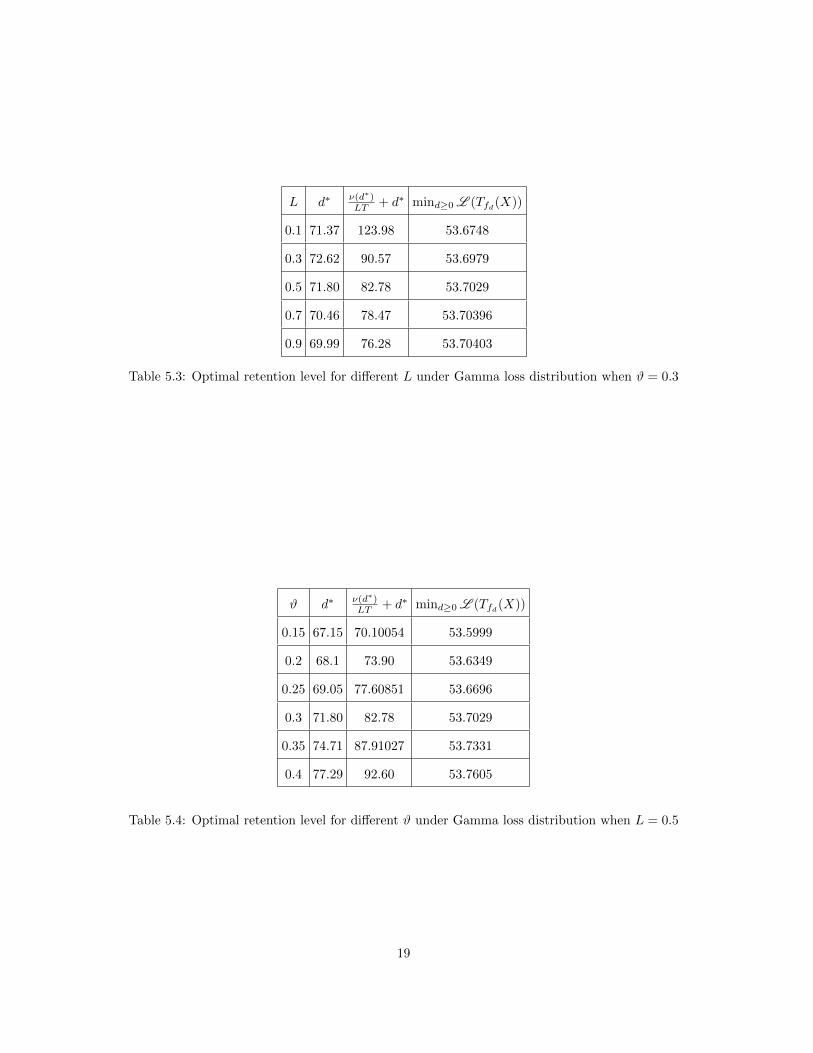
Similar to the Pareto example, the risk-adjusted value of liability increases with the loss con-

version factor L while both the risk-adjusted value of liability and the optimal retention level

increase with the loading coefficient ϑ for the Gamma loss distribution. It is also of interest to

study the effect of the tail behaviour of a loss distribution on the optimal insurance model. In

particular, L (Tfd∗ (X)) and d∗ for Gamma distribution are larger than the corresponding values

for the heavy tailed Pareto distribution although both distributions have same mean and variance.

This suggests that when an insured faces a risk that has a heavy tail, it would cede more risk to

an insurer and result in a lower risk-adjusted value of liability.

18

L d∗ ν(d∗)LT + d∗ mind≥0 L (Tfd(X))

0.1 71.37 123.98 53.6748

0.3 72.62 90.57 53.6979

0.5 71.80 82.78 53.7029

0.7 70.46 78.47 53.70396

0.9 69.99 76.28 53.70403

Table 5.3: Optimal retention level for different L under Gamma loss distribution when ϑ = 0.3

ϑ d∗ ν(d∗)LT + d∗ mind≥0 L (Tfd(X))

0.15 67.15 70.10054 53.5999

0.2 68.1 73.90 53.6349

0.25 69.05 77.60851 53.6696

0.3 71.80 82.78 53.7029

0.35 74.71 87.91027 53.7331

0.4 77.29 92.60 53.7605

Table 5.4: Optimal retention level for different ϑ under Gamma loss distribution when L = 0.5

19

6 Concluding remarks

In this paper, we study the design of an optimal retrospective rating plan from the perspective of

an insured under a criterion that preserves the convex order. We find that the insured would suffer

more risk exposure for a larger loss conversion factor or a higher loading coefficient in maximum

premium. Moreover, it is shown that any admissible insurance contract is dominated by a stop-

loss policy. Further, the optimal retention of stop-loss insurance is derived numerically under

the criterion of minimizing the risk-adjusted value of the insured’s liability where the liability

valuation is carried out by a cost-of-capital approach based on CVaR risk measure.

To simplify the analysis, we make some rather stringent assumptions on the retrospective

premium principle in this paper. For example, we set the minimum premium to be zero and the

maximum premium to be proportional to the expected value of indemnity. Moreover, the basic

premium is assumed to be a solution to Equation (1.3). In practice, the retrospective rating

plan may have a much more complicated pricing mechanism. Therefore, it will be of significant

interest to study the optimal design of retrospective rating plan with more general retrospective

premium principle. We leave this for future research exploration.

Acknowledgement

Tan acknowledges the financial support from the Natural Sciences and Engineering Research

Council of Canada (No: 368474), and Society of Actuaries Centers of Actuarial Excellence Re-

search Grant.

References

Arrow, K.J., 1963. Uncertainty and the welfare economics of medical care. American Economic

Review 53(5), 941-973.

Artzner, P., Delbaen, F., Eber, J.M., Heath, D., 1999. Coherent measures of risk. Mathematical

Finance 9(3), 203-228.

Asimit, A.V., Badescu, A.M., Verdonck, T., 2013. Optimal risk transfer under quantile-based risk

measurers. Insurance: Mathematics and Economics 53(1), 252-265.

Balbas, A., Balbas, B., Heras, A., 2009. Optimal reinsurance with general risk measures. Insur-

ance: Mathematics and Economics 44(3), 374-384.

Bernard, C., Tian, W., 2009. Optimal reinsurance arrangements under tail risk measures. The

Journal of Risk and Insurance 76(3), 709-725.

Borch, K., 1960. An attempt to determine the optimum amount of stop loss reinsurance. In:

Transactions of the 16th International Congress of Actuaries, vol. I, pp. 597-610.

Cai, J., Tan, K.S., 2007. Optimal retention for a stop-loss reinsurance under the VaR and CTE

risk measures. Astin Bulletin 37(1), 93-112.

20

Cai, J., Tan, K.S., Weng, C., Zhang, Y., 2008. Optimal reinsurance under VaR and CTE risk

measures. Insurance: Mathematics and Economics 43(1), 185-196.

Cheung, K.C., 2010. Optimal reinsurance revisited—a geometric approach. Astin Bulletin 40(1),

221-239.

Chi, Y., 2012. Reinsurance arrangements minimizing the risk-adjusted value of an insurer’s lia-

bility. Astin Bulletin 42(2), 529-557.

Chi, Y., Lin, X.S., 2014. Optimal reinsurance with limited ceded risk: A stochastic dominance

approach. Astin Bulletin 44(1), 103-126.

Chi, Y., Tan, K.S., 2011. Optimal reinsurance under VaR and CVaR risk measures: A simplified

approach. Astin Bulletin 41(2), 487-509.

Cong, J., Tan, K.S., 2014. Optimal VaR-based risk management with reinsurance. Annals of

Operations Research, in press.

Dhaene, J., Denuit, M., Goovaerts, M.J., Kaas, R., Vyncke, D., 2002. The concept of comono-

tonicity in actuarial science and finance: theory. Insurance: Mathematics and Economics 31(1),

3-33.

European Commission 2009. Directive 2009/138/EC of the European Parliament and of the Coun-

cil of 25 November 2009 on the Taking-up and Pursuit of the Business of Insurance and Rein-

surance (Solvency II). Official Journal of the European Union L335.

Follmer, H., Schied, A., 2004. Stochastic Finance: An Introduction in Discrete Time, second

revised and extended edition. Walter de Gruyter.

Gajek, L., Zagrodny, D., 2004. Optimal reinsurance under general risk measures. Insurance: Math-

ematics and Economics 34(2), 227-240.

Gollier, C., Schlesinger, H., 1996. Arrow’s theorem on the optimality of deductibles: A stochastic

dominance approach. Economic Theory 7(2), 359-363.

Kaluszka, M., 2001. Optimal reinsurance under mean-variance premium principles. Insurance:

Mathematics and Economics 28(1), 61-67.

Kaluszka, M., Okolewski, A., 2008. An extension of Arrow’s result on optimal reinsurance con-

tract. The Journal of Risk and Insurance 75(2), 275-288.

Meyers, G.G., 2004. Retrospective premium. In Encyclopedia of Actuarial Science, vol 3, ed. J.

Teugels and B. Sundt. John Wiley& Sons.

Ohlin, J., 1969. On a class of measures of dispersion with application to optimal reinsurance.

Astin Bulletin 5(2), 249-266.

Raviv, A., 1979. The design of an optimal insurance policy. American Economic Review 69(1),

84-96.

21

Shaked, M., Shanthikumar, J. G., 2007. Stochastic Orders. Springer, New York.

Swiss Federal Office of Private Insurance, 2006. Technical document on the Swiss Solvency Test.

FINMA.

Van Heerwaarden, A.E., Kaas, R., Goovaerts, M.J., 1989. Optimal reinsurance in relation to

ordering of risks. Insurance: Mathematics and Economics 8(1), 11-17.

Young, V.R., 1999. Optimal insurance under Wang’s premium principle. Insurance: Mathematics

and Economics 25(2), 109-122.

22