
The Design and Optimization of Segmentally Precast...
251
.. - TECHNICAL REPORT STANDARD TITLE PAGE 1. Report No. 2. Government Accession No. 3. Recipient's Cotolog No. CFHR 3-5-69-121-3 4. Title ond Subtitle S. Report Dote THE DESIGN AND OPTIMIZATION OF SEGMENTALLY PRECAST PRESTRESSED BOX GIRDER BRIDGES Augus t 1975 6. Performing Orgoni zotion Code 7. Author'sl B. Performing Orgonizotion Report No. G. C. Lacey and J. E. Breen Research Report 121-3 9. Performing Organizotion Nome and Addre .. 10. Work Unit No. Center for Highway Research 11. Controct or Grant No. Research Study 3-5-69-121 The University of Texas at Austin Austin, Texas 78712 13. Type of Report and Period Cover.d 12. Sponsoring Agency Nome and Addr ... Texas State Department of Highways and Public Transportation Transportation Planning Division P. O. Box 5051 Austin, Texas 78763 1S. Supplementory Notes Interim 14. Sponaoring Agency Code Study conducted in cooperation with the U.S. Department of Transportation, Federal Highway Administration. Research Study Title: Procedures for Long Span Prestressed Concrete Bridges of Segmental Construction" 16. Abatract The economic advantages of precasting can be combined with the structural efficiency of prestressed concrete box girders for long span bridge structures when erected by segmental construction. The complete superstructure is precast in box segments of convenient size for transportation and erection. These precast seg- ments are erected in cantilever and post-tensioned together to form the complete superstructure. This report details the application of design, analysis, and optimization techniques to segmentally precast prestressed concrete box girder bridges. These were classified into two main types according to their method of construction, namely those constructed on falsework and those erected in cantilever. Design procedures are developed for both types of construction. Both ultimate strength and service load design criteria are satisfied under all loading cond i tions . Sample designs are carried out for the case of a hypothetical two-span bridge constructed on falsework and that of an actual three-span bridge erected in cantilever. Optimization techniques are used to find the optimal cross sections, i.e., those having minimum cost for such bridges. 17. Key Words bridges, segmentally precast, pre- stressed, box girder design, analysis lB. Distribution Statement No restrictions. This document is avail- able to the public through the National Technical Information Service, Spring- field, Virginia 22161. 19. Security Clouif. (of thia report) 20. Security ClaasH. (of thi s pagel 21. No. of Pages 22. Price Unclassified Unc1as s ified 250 Form DOT F 1700.7 (8-61)
Transcript of The Design and Optimization of Segmentally Precast...

..
-
TECHNICAL REPORT STANDARD TITLE PAGE
1. Report No. 2. Government Accession No. 3. Recipient's Cotolog No.
CFHR 3-5-69-121-3
4. Title ond Subtitle S. Report Dote
THE DESIGN AND OPTIMIZATION OF SEGMENTALLY PRECAST PRESTRESSED BOX GIRDER BRIDGES
Augus t 1975 6. Performing Orgoni zotion Code
7. Author'sl B. Performing Orgonizotion Report No.
G. C. Lacey and J. E. Breen Research Report 121-3
9. Performing Organizotion Nome and Addre .. 10. Work Unit No.
Center for Highway Research 11. Controct or Grant No.
Research Study 3-5-69-121 The University of Texas at Austin Austin, Texas 78712
13. Type of Report and Period Cover.d ~~~----~--~--~~--------------------------~ 12. Sponsoring Agency Nome and Addr ...
Texas State Department of Highways and Public Transportation
Transportation Planning Division P. O. Box 5051 Austin, Texas 78763
1 S. Supplementory Notes
Interim
14. Sponaoring Agency Code
Study conducted in cooperation with the U.S. Department of Transportation, Federal Highway Administration. Research Study Title: '~esign Procedures for Long Span Prestressed Concrete Bridges of Segmental Construction"
16. Abatract
The economic advantages of precasting can be combined with the structural efficiency of prestressed concrete box girders for long span bridge structures when erected by segmental construction. The complete superstructure is precast in box segments of convenient size for transportation and erection. These precast segments are erected in cantilever and post-tensioned together to form the complete superstructure.
This report details the application of design, analysis, and optimization techniques to segmentally precast prestressed concrete box girder bridges. These were classified into two main types according to their method of construction, namely those constructed on falsework and those erected in cantilever.
Design procedures are developed for both types of construction. Both ultimate strength and service load design criteria are satisfied under all loading cond i tions .
Sample designs are carried out for the case of a hypothetical two-span bridge constructed on falsework and that of an actual three-span bridge erected in cantilever.
Optimization techniques are used to find the optimal cross sections, i.e., those having minimum cost for such bridges.
17. Key Words
bridges, segmentally precast, prestressed, box girder design, analysis
lB. Distribution Statement
No restrictions. This document is available to the public through the National Technical Information Service, Springfield, Virginia 22161.
19. Security Clouif. (of thia report) 20. Security ClaasH. (of thi s pagel 21. No. of Pages 22. Price
Unclassified Unc1as s ified 250
Form DOT F 1700.7 (8-61)

!!!!!!!!!!!!!!!!!!!"#$%!&'()!*)&+',)%!'-!$-.)-.$/-'++0!1+'-2!&'()!$-!.#)!/*$($-'+3!
44!5"6!7$1*'*0!8$($.$9'.$/-!")':!

THE DESIGN AND OPTIMIZATION OF SEGMENTALLY PRECAST PRESTRESSED BOX GIRDER BRIDGES
by
G. C. Lacey
and
J. E. Breen
Research Report No. 121-3
Research Project No. 3-5-69-121
"Design Procedures for Long Span Prestressed Concrete Bridges of Segmental Construction"
Conducted for
The Texas Highway Department In Cooperation with the
U. S. Department of Transportation Federal Highway Administration
by
CENTER FOR HIGHWAY RESEARCH THE UNIVERSITY OF TEXAS AT AUSTIN
August 1975

The contents of this report reflect the views of the authors, who are responsible for the facts and the accuracy of the data presented herein. The contents do not necessarily reflect the official views or policies of the Federal Highway Administration. This report does not constitute a standard, specification, or regula tion.
ii
.-

PRE F ACE
This report is the third of a series which summarizes the detailed
investigation of the various problems associated with the design and con
struction of long span prestressed concrete bridges of precast segmental
construction. The initial report in this series summarized the general
state-of-the-art for design and construction of this type bridge as of
May 1969. The second report stated requirements for and reported test
results of epoxy resin materials for jointing large precast segments. This
report summarizes design criteria and procedures for bridges of this type
and includes two design examples. One of these examples is the three-span
segmental bridge constructed in Corpus Christi, Texas, during 1972-73.
Later reports in this series will detail the development of an incremental
analysis procedure and computer program which can be used to analyze seg
mentally erected box girder bridges and will summarize the results of an
extensive physical test program of a one-sixth scale model of the Corpus
Christi structure. Comparisons with analytical results using the computer
model and verification of the design procedures will be presented in those
reports.
This work is a part of Research Project 3-5-69-121, entitled "Design
Procedures for Long Span Prestressed Concrete Bridges of Segmental Construc
tion." The studies described were conducted as a part of the overall
research program at The University of Texas at Austin, Center for Highway
Research. Work was sponsored jointly by the Texas Highway Department and
the Federal Highway Administration under an agreement with The University
of Texas at Austin and the Texas Highway Department.
Liaison with the Texas Highway Department was maintained through
the contact representative, Mr. Robert L. Reed, and the State Bridge Engineer
Mr. Wayne Henneberger. Extensive detailed liaison in the design phase was
maintained with Mr. Harold J. Dunlevy and Mr. Alan B. Matejowsky of the
Bridge Division; Mr. Donald E. Harley and Mr. Robert E. Stanford were the
contact representatives for the Federal Highway Administration.
iii

The overall study was directed by Dr. John E. Breen, Professor of
Civil Engineering. He was assisted by Dr. Ned H. Burns, Professor of
Civil Engineering. The design phase and the optimization studies were
developed by Dr. Geoffrey C. Lacey, who at that time was a Research Engi
neer for the Center for Highway Research. Valuable assistance was con
tributed by Dr. Robert C. Brown, Jr., Dr. Satoshi Kashima, and Mr. Tsutomu
Komura, Assistant Research Engineers, Center for Highway Research. The
authors are appreciative of the contributions of Dr. D. M. Himmelblau
and Dr. W. G. Lesso of the College of Engineering, The University of
Texas at Austin, for their advice regarding optimization techniques.
iv

SUM MAR Y
The economic advantages of precasting can be combined with the
structural efficiency of prestressed concrete box girders for long span
bridge structures when erected by segmental construction. The complete
superstructure is precast in box segments of convenient size for trans
portation and erection. These precast segments are erected in cantilever
and post-tensioned together to form the complete superstructure.
This report details the application of design, analysis, and
optimization techniques to segmentally precast prestressed concrete box
girder bridges. These were classified into two main types according to
their method of construction, namely those constructed on falsework and
those erected in cantilever. The prestressing cable patterns and the design
procedures required are very different in the two types of construction.
Design procedures are developed for both types of construction.
Both ultimate strength and service load design criteria are satisfied
under all loading conditions. The effect of the cable force on the con
crete section is calculated u~ing an equivalent load concept. A computer
program is used to check all service level stresses.
Sample designs are carried out for the case of a hypothetical
two-span bridge constructed on falsework and that of an actual three-span
bridge erected in cantilever. In the former case, full length draped
cables are used, the profile consisting of three parabolas. In the case
of the bridge erected in cantilever, each stage of construction is a
separate design condition and a pattern of cables of varying lengths is
required.
Optimization techniques are used to find the optimal cross sections,
i.e., those having minimum cost for such bridges. In each case, the
problem is treated as an unconstrained nonlinear programming problem and
a subroutine is developed to compute the objective function. Numerical
v

methods of solution that do not require derivatives of the objective
function are used. From contour plots of the objective function it is
found that the optimal dimensions can be varied substantially with small
increase in cost.
vi
IMP L E MEN TAT ION
This report presents the background and detail of design,
analysis, and optimizing procedures recommended for use with precast
segmental prestressed concrete box girders erected on fa1sework or by
balanced cantilevering. The design procedures illustrate the use of
both ultimate strength and service load design techniques and consider
a wide range of loading conditions. The interaction of manual calcula
tions and various computerized analysis procedures is illustrated. The
report includes a brief summary of important factors to be considered in
in i t ia 1 design, trea ts analytical procedures which are especially
useful in dealing with the types of tendon layouts and erection schemes
utilized with this construction, and provides two major example problems
illustrating the numerical calculations and procedures to be utilized.
One of the example problems is based on the box girder bridge erected
over the Intracoastal Waterway at Corpus Christi, Texas, and is essen
tially a documentation of the preliminary design procedure used in devel
opment of the structure.
While the design examples consider box girders of constant depth,
the minor variations required in dealing with members of variable depths
are indicated. The design and analysis procedures should be extremely
useful in analysis of proposed structures in the 100 to 300 ft. span
range, can be easily extended to structures up to 450 ft. and can deal
with a wide variety of cross sections.
vii

CON TEN T S
Chapter
1 INTRODUCTION .
1.1 General ....... . 1.2 Segmental Construction 1.3 Research Program in Segmentally Constructed
Bridges .... 1.4 Objective and Scope of this Report
2 DESIGN PROCEDURES
2.1 General . . . 2.2 State-of-the-Art 2.3 Design Sequence. 2.4 Conceptual Design 2.5 Preliminary Design 2.6 Detailed Analysis . 2.7 Verification Analysis. 2.8 Field Support .... 2.9 Change Order Evaluation
2.10 Pier Design ..... . 2.11 Applicable Specifications and Regulations
3 DESIGN PROCEDURE FOR BRIDGES CONSTRUCTED ON FALSEWORK
3.1 Equivalent Load Concept .... 3.2 Design Example - Two-Span Bridge 3.3 Construction Procedure 3.4 Material Properties ... 3.5 Cross Section and Reinforcement 3.6 General Design Criteria .. 3.7 Design of Superstructure .... 3.8 Summary of Design Procedure .. 3.9 Other Examples of Bridges Constructed on
Falsework . . . . . .
4 DESIGN PROCEDURE FOR BRIDGES CONSTRUCTED IN CANTILEVER .............. .
4.1 4.2 4.3 4.4
Equivalent Load of a Cable System. Design Example - Three-Span Bridge Construction Procedure Material Properties ...
viii
Page
1
1 4
10 10
13
13 14 15 17 20 26 27 28 28 28 29
31
32 36 39 40 40 41 42 65
66
69
70 75 78 81

Chapter
5
6
7
8
4.5 4.6 4.7
4.8 4.9
4.10
Design of Cross Section and Reinforcement . General Design Criteria ......... . Design of Superstructure during Cantilever
Construction ......... . Design of Completed Superstructure Summary of Design Procedure . . . . Other Examples of Bridges Constructed in
Cantilever
METHODS OF OPTIMIZATION
5.1 5.2 5.3
5.4
Notation and Definitions Unconstrained Minimization Using Derivatives Unconstrained Minimization without Using
Derivatives ...... . Limitations of the Methods
OPTIMIZATION OF BRIDGES CONSTRUCTED ON FALSEWORK
6.1 First Example--Two-span, Double Box Girder
Page
81 86
86 95
125
133
135
136 136
138 141
145
Bridge . . . . . . . 146 6.2 The Objective Function . . . . 148 6.3 The Optimal Solution . . . . 157 6.4 Second Example--Two-span, Multi-cell Box Girder
Bridge . . . . . .. .......... 162 6.5 The Optimal Solution as a Basis for Design 167 6.6 Possible Limitations of the Optimal Solution 167 6.7 Other Examples for Optimization. ..... 168
OPTIMIZATION OF BRIDGES CONSTRUCTED IN CANTILEVER
7.1
7.2 7.3 7.4 7.5
Example Case--Three-span Double Box Girder Bridge . . . . . . .
The Objective Function ... . The Optimal Solution ... . Effectiveness of the Optimization Techniques Other Examples for Optimization
CONCLUSIONS
8.1 8.2 8.3
General Conclusions . . Particular Conclusions Recorrnnendations
169
169 171 177 181 182
185
185 187 189
REFERENCES
APPENDIX A.
APPENDIX B.
PROTOTYPE BRIDGE PLANS
LISTING OF PROGRAM BOX2 TO CALCULATE SECTION PROPERTIES OF DOUBLE BOX GIRDER BRIDGE
191
195
207
ix
Chapter Page
APPENDIX C. OPTIMIZING PROGRAMS and SUBROUTINES TO CALCULATE OBJECTIVE FUNCTIONS 213
C.1 OPTMSE. . . . 214 C.2 SIMPLEX 221 C.3 Objective Function 2 Span Bridge 225 C.4 Objective Function Mu1tiweb 2 Span Bridge 228 C.S Objective Function 3 Span Bridge . . . .. 230
x
LIS T o F TABLES
Table Page
3.1 Section Properties of Superstructure--Two-Span Bridge 43
4.1 Section Properties of Superstructure--Three-Span Bridge 88
4.2 Top Cable Eccentricities 88
4.3 Top Cables Required 92
4.4 Top Cables Adopted . 94
6.1 Optimal Solution for Two-Span Double Box Girder Bridge 159
6.2 Optimal Solution for Two-Span Three-Cell Box Girder Bridge . . • .. .. . . . . . . . 164
7.1 Optimal Solution for Three-Span Double Box Girder Bridge . . . .. ......... ... . 178
xi
LIS T o F FIG U RES
Figure Page
1.1 Typical cellular cross section . . . . . . . 2
1.2 Superstructure of the Oostersche1de Bridge, The Ne ther1and s . . . . . . . . 5
1.3 Girder cross-sectional configurations 6
1.4 Construction of complete span 8
2.1 Interactive design sequence 16
2.2 Types of longitudinal profiles 18
2.3 Box girder cross section types 21
2.4 Span/depth ratios 22
2.5 (Bending moment/span) versus span in various countries 23
2.6 (a) Web thickness parameter at piers (b) Corpus Christi Bridge parameter calculations 25
2.7 Usage of basic section types . • 26
2.8 Provisions for unbalanced moment 30
3.1 Equivalent cable load 34
3.2 Parabolic cable 34
3.3 Straight cable . 34
3.4 Cable anchorage point 34
3.5 Elevation of two-span bridge 37
3.6 Cross section of superstructure 38
3.7 Cable profile 46
3.8 Idealized cable profile 46
xii

Figure
3.9 Equivalent cable loads on superstructures
3.10 Variation in position of section centroid
3.11 Idealized maximum sections
3.12 Idealized minimum sections
3.13 MUPDI analysis of stress distributions in two-span bridge at pier . . . . . . . . . . . . . . . . . .
3.14 MUPDI analysis of stress distributions in two-span bridge at 70 ft. from end support
3.15 MUPDI analysis live load stress distribution in two-span bridge at 70 ft. from end support under live load on one side only ...
3.16 Cable and reinforcement details
4.1 Moment balancing for a uniform load
4.2 Equivalent load of a cable system
4.3 Elevation of three-span bridge.
4.4 Cross section of superstructure
4.5 Suggested improvement for temporary support
4.6 Stages of Construct~on ..
4.7 Cantilever portion of deck slab
4.8 Main span bottom cable pattern in preliminary design
4.9 Equivalent load for main span bottom cables
4.10 Equivalent load for side span bottom cables
4.11 Idealized maximum sections
4.12 Idealized minimum sections
4.13 Elevation showing design cable profile
4.14 Design cable and reinforcement details.
xiii
Page
49
49
58
59
60
61
63
64
71
74
76
77
79
80
83
83
103
106
116
117
119
120

Figure
4.15
4.16
4.17
4.18
4.19
4.20
4.21
4.22
5.1
5.2
6.1
6.2
6.3
6.4
6.5
7.1
7.2
B.1
MUPDI analysis stress distributions in three-span bridge at main pier . . . . . . . . . . . . . . .
MUPDI analysis stress distributions in three-span bridge at center of main span
Stress envelopes during erection (ksi)
(a) Stress distribution at completion (ksi) (b) Stress at pier section at completion of Stage 6 -
comparison to beam theory (ksi) ••..•...
Variation of average top flange stress at pier section
Variation of average bottom flange stress at pier section
Intracoastal Canal Bridge--disp1acements during erection
Elastic curve at various stages of closure
Local and global optimal solutions
Flow chart for the Nelder-Mead method
Cross section of first example
Profile of roadway embankment
Objective function contours for two-span double box girder bridge ...... .
Cross section of second example
Objective function contours for two-span three-cell box girder bridge . . . . . . . . . .
Cross section of example for cantilever erection •
Objective function contours for three-span double box girder bridge
Notation for Program BOX2
xiv
Page
121
122
126
127
128
129
130
131
137
142
147
147
160
163
166
170
179
209

a
b
b'
d a
d ec
d m
e
f~
f c
t c
fd f pc
f pe
f s
f' s
f se
= =
=
=
=
= =
= =
NOT A T ION
depth of concrete stress block (Chapter 4)
average concrete section area (Chapters 6 and 7)
minimum concrete section area
maximum concrete section area
area of prestressing cables or unprestressed reinforcement
area of web reinforcement
width of compression face of member (Chapters 3 and 4)
width of superstructure (Chapters 6 and 7)
total width of girder webs
widths of superstructure elements
width of lower lab of box
width of deck slab per box
objective function
distance from compression edge to centroid of cables or reinforcement (Chapters 3 and 4)
depth of girder (Chapters 2, 6, and 7)
depth of stress block
cable eccentricity
distance between center of compression and cable centroid
cable eccentricity
objective function
compressive stress in concrete
compressive strength of concrete
stress at top of girder due to dead load
compressive stress at centroid of girder
compressive stress at top of girder due to prestress
stress in steel
ultimate strength of prestressing steel
effective steel prestress after losses
xv

f su f
t
f y
f*
F
h
I
j
k
y
M
M cr
n w p
p
p
q
R
s
s t
u
v
v c
v p
V u
w
=
= = = = = =
=
= = = = = = = =
= =
= = =
= =
= = = = =
calcu~ed stress in prestressing steel at ultimate load
stress at top of girder
yield stress of unprestressed reinforcement
yield point stress of prestressing steel
cable force
cable drape
moment of inertia
ratio of distance between center of compression and center of tension to the effective depth, d
ratio of distance between compression edge of slab and neutral axis to the effective depth, d
slab stiffnesses
concentrated moment from cable
bending moment
flexural cracking moment
primary cable moment
resultant cable moment
secondary cable moment
ultimate moment
number of webs of girder
A /bd s
transverse force or load
cable force at ultimate load
fraction of span over which bottom slab is thickened
concrete moment resistance coefficient
longitudinal spacing of web reinforcement (Chapters 3 and 4)
sloping height of web between slabs (Chapters 6 and 7)
effective span of deck slab
thickness of slab
shear force
shear carried by concrete
vertical component of cable force
shear at ultimate load
load per unit length
xvi

x = horizontal coordinate
x.(i=l,n) = variables 1
x column vector of variables
y vertical coord ina te
z = ratio of distance between pier center and section considered to the span
Ii = cable slope
(f) = capacity reduction factor
xvii

C HAP T E R 1
INTRODUCTION
1.1 General
Bridge engineers continually face requirements for safer, more
economical bridge structures. In response to many requirements imposed
by traffic considerations, natural obstacles, more efficient use of land
in urban areas, safety, and aesthetics, the trend is to longer span
structures. At present, the most commonly used structural system for
highway bridge structures in Texas consists of prestressed concrete
I-girders combined with a cast-in-place deck slab. This system has prac
tical limitations for spans beyond the 120 ft. range. With the fluctuating
costs and maintenance requirements of steel bridges, there exists a need
to develop an economical approach to achieve precast, prestressed con
crete spans in the 120-400 ft. range.
In the United States, spans in the 160 ft. range have been achieved 23*
by the use of post-tensioned, cast-in-place girders. The box, or cellu-
lar, cross section shown in Fig. 1.1 is ideal for bridge superstructures
since its high torsional stiffness provides excellent transverse load
distributing properties. Construction experience along the West Coast
has indicated that this type bridge is a very economical solution to many
long span challenges.
In Europe, Japan, and Australia, during the late 1960's and early
1970's, the advantages of the cellular cross section were combined with
the substantial advantages obtained by maximum use of prefabricated com-20
ponents. By precasting the complete box girder cross section in short
segments of a convenient size for transportation and erection, the entire
*Numbers refer to references listed at the end of this report.
1

2
Fig. 1.1. Typical cellular cross section
bridge superstructure may be precast. These precast units are subsequently
assembled on the site by post-tensioning them longitudinally. A number
of extremely long span precast and cast-in-p1ace box girder bridges have 16 20
been segmentally constructed in Europe ' and interest in this construc-
tion concept is rapidly growing in the United States. A three-span
precast segmentally constructed box girder bridge with a 200 ft. maximum
span was completed in Corpus Christi, Texas, in 1973.
When construction of large numbers of prestressed concrete bridges
is envisaged, precasting has a number of advantages over cast-in-p1ace
construction, e.g.
(1) Mass production of standardized girder units is possible. This
isdone at present with precast I-girders for shorter spans.
(2) High quality control can be attained through plant production
and inspection.
(3) Greater economy of production is possible by precasting the girder
units at a plant site rather than casting in place.
(4) The speed of erection can be much greater. This is very
important when construction interferes with existing traffic
and is most critical in an urban environment.
In segmental box girder construction utilizing the cantilever erec
tion procedure, precasting has several other advantages over cast-in-p1ace
construction, e.g.
(1) Strength gain of the concrete is essentially taken out of the
erection critical path. This allows faster erection times and
higher concrete strength at time of stressing.

(2) Shrinkage strains can substantially develop prior to erection
and stressing if adequate lead times and stockpiling are used.
(3) Creep rates can be substantially reduced since the segments are
considerably more mature at time of stressing.
The major advantages frequently cited for utilization of cast
in-place segmental construction are:
(1) Provision of positive nonprestressed reinforcement across the
joints is easier.
(2) Continuous correction of girder grade and line is possible to
compensate for deformations.
Extensive utilization of epoxy joints, grouted tendons, and
3
shear keys has reduced the emphasis on the positive bonded joint rein
forcement while the versatility of the match casting procedure on numerous
major projects involving complex horizontal and vertical alignment has
illustrated the ability of the precast procedures to deal with geometri
cal problems.
At present, precast I-section girders are widely used in highway
bridge construction for spans up to about 120 ft. They are cast in a
manufacturing plant and transported to the bridge site for erection.
While their span can be stretched by using "drop in" girders, they cannot
be used for significantly greater spans, because this length is approxi
mately the upper limit that can be transported by road. In addition,
I-sections are not the most structurally suitable form for long span
bridge structures. A better structural unit is the box girder.
The box girder is a very compact structural member, which combines
high flexural strength with high torsional strength and stiffness. It is
superior to the I-section girder for long spans in that (a) there is no
lateral buckling problem so that the compressive capacity of the bottom
flange is fully utilized, and (b) the torsional rigidity brings about a
more even distribution of flexural stresses across the section, under a
variety of live loads. A further advantage of the box girder in precast

4
structures is that it is possible to precast the full cross section
(apart from a longitudinal joining strip in some cases), whereas with
I-sections the deck slab must largely be cast in place.
A considerable number of long span bridges have been constructed
throughout the world using prestressed concrete box girders. Both cast
in-place construction and segmental precasting have been widely utilized.
The suitability of box girders even for extremely long spans can be seen
from the Bendorf Bridge in West Germany, which was cast in place and has
a span of 682 ft. In the United States, cast-in-place box girder bridges
are being widely used by the California Division of Highways, as well as
in several other states.
When box girder bridges are precast, the casting is generally
segmental, i.e., the girders are cast in short, full width units or
"segments". The reason for manufacture in short segments is essentially
that box girders, unlike I-girders which have narrow width, cannot be
readily transported in long sections. In addition, the short units are
suited to fairly simple methods of assembly and post-tensioning. During
erection the segments are joined together, end to end, and post-tensioned
to form the completed superstructure. The segmental pattern for a typical
bridge is shown in Fig. 1.2. The length and weight of the segments are
chosen so as to be most suitable for tr~nsportation and erection.
1.2 Segmental Construction
Figure 1.3 illustrates some of the wide range of cross-sectional
shapes which can be used. Various techniques have been used for jointing
between the precast segments, with thin epoxy resin joints being the widest
used. The most significant variation in construction technique is the
method employed to assemble the precast segments. The most widely used
methods may be categorized as construction on falsework and cantilever
construction. Construction on falsework is the simplest method of erecting
precast, segmental bridges. It also leads to the simplest design approach.
The joints used are usually cast-in-place concrete or mortar. This method
is particularly applicable to locations where access by construction

Fig. l.a. Superstructure of the Oosterschelde Bridge, The Netherlands

6
(a) Single cell girder
, , I
\ J \ J
(b) Single cells joined by deck
(c) Multicell girder
Fig. 1.3. Girder cross-sectional configurations

7
equipment is difficult, the project is of limited scope and traffic
interruptions due to falsework are acceptable, and where single or twin
spans are to be used so that balanced cantilevering is not feasible. The
prestressing system for the superstructure will normally consist of long
draped cables in the box girder webs. If the overall length of the bridge
is moderate, it is possible to set all the segments in place and join them
before inserting and tensioning full length cables. This method tends to
economize on prestressing steel and hardware. Stressing operations are
minimized but at the expense of falsework costs.
The outstanding advantage of the cantilever approach to segmental
construction lies in the fact that the complete construction may be accom
plished without the use of falsework and hence minimizes traffic
in terrup tion.
Assembly of the segments is accomplished by sequential balanced
cantilevering outward from the piers toward the span centerlines. Ini
tially the "hannnerhead" is formed by erecting the pier segment and
attaching it to the pier to provide unbalanced moment capacity. The two
adjoining segments are then erected and post-tensioned through the pier
segment, as shown in Fig. 1.4(a). Auxiliary supports may be employed for
added stability during cantilevering or to reduce the required moment
capacity of the pier. Each stage of cantilevering is accomplished by
applying the epoxy resin jointing material to the ends of the segments,
lifting a pair of segments into place, and post-tensioning them to the
standing portion of the structure [see Fig. 1.4(b)]. Techniques for
positioning the segments vary. They may be lifted into position by means
of a truck or floating crane, by a traveling lifting device attached to
(or riding on) the completed portion of the superstructure, or by using
a traveling gantry. In the latter case the segments are transported over
the completed portion of the superstructure to the gantry and then lowered
in tv position.
The stage-by-stage erection and prestressing of precast segments
is continued until the cantilever arms extend nearly to the span center
line. In this configuration the span is ready for closure. The term

Epoxy resin jOint
Anchor bolts or prestressinc;a
7
Pier segment
(a) Construction of hammerhead
(b) Segmental cantilevering
tendons
"'4.-__ Adjustinc;a jacks
(c) Closure of span
Fig. 1.4. Construction of complete span
00

9
closure refers to the steps taken to make the two independent cantilever
arms between a pair of piers one continuous span. In earlier segmentally
constructed bridges there was no attempt to ensure such longitudinal con
tinuity. At the center of the span, where the two cantilever arms meet,
a hinge or an expansion joint was provided. This practice has been largely
abandoned in precast structures, since the lack of continuity allows 19 24 unsightly creep deflections to occur.' Ensuring continuity is advised
and usually involves:
(1) Ensuring that the vertical displacements of the two cantilever ends are essentially equal and no sharp break in end slope exists.
(2) Casting in place a full width closure strip, which is generally from 1 to 3 ft. in length.
(3) Post-tensioning through the closure strip to ensure structural continuity.
The exact procedures required for closure of a given structure must be
carefully specified in the construction sequence. The final step in
closure is to adjust the distribution of stress throughout the girder to
ensure maximum efficiency of prestress. Adjustment is usually necessary
to offset undesirable secondary moments induced by continuity prestressing.
The final adjustments may invo1ve19
(1) Adjusting the elevation of the girder soffit, at the piers, to induce supplementary moments. The adjustment may be accomplished by means of jacks inserted between the pier and the soffit of the girder with subsequent shimming to hold the girder in position.
(2) Insertion of a hinge in the gap between the two cantilever arms to reduce the stiffness of the deck while the continuity tendons are partially stressed. The hinge is subsequently concreted before the continuity tendons are fully stressed.
(3) A combination of hinges and jacks inserted in the gap to control the moment at the center of the span while the continuity tendons are stressed. The final adjustment is made by further incrementing the jack force and finally concreting the joint in.
The first of these possibilities is the widest used. After final
adjustments are complete, the operation is moved forward to the next pier
and the erection sequence begins again.

10
1.3 Research Program in Segmentally Constructed Bridges
In 1969, a comprehensive research effort dealing with segmental
construction of precast concrete box girder bridges was initiated at The
University of Texas at Austin. This report summarizes part of this
mu1tiphase project which had the following objectives:
(1) To investigate the state-of-the-art of segmental bridge construction.
(2) To establish design procedures and design criteria in general conformance with provisions of existing design codes and standards.
(3) To develop optimization procedures whereby the box girder cross section dimensions could be optimized with respect to cost to assist preliminary design.
(4) To develop a mathematical model of a prestressed box girder, and an associated computer program for the analysis of segmentally constructed girders during all stages of erection.
(5) To verify design and analysis procedures using a highly developed structural model of a segmental box girder bridge.
(6) To verify model techniques by observance of construction and service load testing of a prototype structure.
Various phases of this work were reported in previous reports in 7-11 14-16
this series and in several dissertations.' Objective (1) was
initially accomplished with publication of Report 121-1. It has subse
quently been updated and advanced by Muller's excellent paper. 20 Objec
tives (2) and (3) are the direct areas of interest in the present report.
Objective (4) was accomplished with the development of the program SIMPLA2
as documented in Report 121-4. Objectives (5) and (6) were accomplished
as documented in Report 121-5.
1.4 Objectives and Scope of this Report
The object of this report is to document proper design procedures
and to develop practical optimization techniques for the application of
the segmentally precast box girder in long span highway bridge superstructures.
Segmentally precast box girders should be designed and analyzed con
sidering the construction process. In contrast to many concrete structures,

11
it is essential that erection conditions and stresses be carefully checked
at all stages for balanced cantilever construction. Analysis at each
stage can represent a monumental task unless the problem is simplified
considerably. Effects of simplification for purposes of design are often
difficult to evaluate, since the degree to which a box girder behaves as
an element depends on many variables and it is difficult to determine.26
In developing the design procedures, the authors used adaptations
of methods recommended in AASHO specifications for the design of normal
bridge cross sections under the action of wheel loads wherever possible.
This AASHO method was somewhat simplified and utilized in the development
of a computerized optimization scheme to determine preliminary box girder
cross section dimensions for minimum cost.
In Chapter 2 a general design procedure is outlined. Interaction
of the various steps of preliminary proportioning, optimization studies,
detailed transverse and longitudinal design, box girder analysis for
warping effects, checks of erection stresses, and development of post
tensioning system details are interrelated. Construction trends influ
encing preliminary proportioning are examined and references are made
to several helpful summaries of physical properties of completed
structures.
Detailed procedures for the design of bridges constructed on
falsework are developed in Chapter 3 and a design example is utilized.
Chapter 4 gives similar material and an example for bridges erected in
cantilever. Both ultimate strength and service load design criteria are
satisfied. Utilization of existing computer programs to thoroughly check
the stresses under various loadings is illustrated.
Mathematical methods of optimization are briefly reviewed in
Chapter 5. Appropriate methods are applied to illustrate factors affecting
the optimal cross section for bridges constructed on falsework (Chapter 6)
and erected in cantilever (Chapter 7). In the optimization studies, the
function which is minimized is an approximate cost index for the bridge.

!!!!!!!!!!!!!!!!!!!"#$%!&'()!*)&+',)%!'-!$-.)-.$/-'++0!1+'-2!&'()!$-!.#)!/*$($-'+3!
44!5"6!7$1*'*0!8$($.$9'.$/-!")':!

C HAP T E R 2
DESIGN PROCEDURES
2.1 General
While over one hundred long span bridges have been constructed
throughout the world using segmentally precast box girders, their utiliza
tion in the United States has been very slow in developing. With comple
tion of the first U.S. project in 1973, there has been a heightened interest
and a number of projects are now actively underway. While there are
undoubtedly many reasons for the slow development of this type of con
struction in the United States, probably one of the most significant
is the general division of the engineering and construction responsibilities
that has existed in the concrete industry. The segmental precast box
girder bridge requires extensive consideration of construction methods
and procedures during the design phase. In the same way, the erector
must be responsible for substantial calculations for control of stresses
and deflections throughout the erection phase. While such interaction has
been very common in construction of long span steel bridges, it has not
been as usual in long span concrete structures.
A successful design of a precast segmental box girder bridge must
consider carefully the constructabi1ity of the project, must leave room for
competitive systems and constructor improvements, and must consider the
stability of the structure in all of its embryo stages as well as per
formance of the completed structure.
Division of responsibility must be very carefully developed, so
that the constructor is not forced into undertaking an unrealistic or unsafe
construction procedure by orders of the designer and, conversely, the
designer is not responsible for errors or lapse in judgment by the contractor.
13

14
The authors feel that the main reason for the lag in development
of this type of structure in the United States has been the technological
transfer gap, not of highly involved analysis procedures, but rather of
efficient construction procedures suited for the engineering, constructor,
laborer, and material practices of the United States.
In this chapter a very brief outline of the design procedures
which should lead to a successful project is given. The material in this
chapter is intended to outline the general framework of the design process.
Two very specific technical designs are included in subsequent chapters
to provide specific guidance on "detailing". Substantial information on
factors affecting optimization of the cross sections are included in sub
sequent chapters to assist in preliminary designs.
2.2 State-of-the-Art
Report 121-1 summarized the state-of-the-art in precast segmental
box girder technology as of 1970. The ensuing five years have seen rapid
developments in this technology. Foreign experience by one of the world's
foremost builders of this type structure was summarized in 1974 at the
FIP/PCI Congress in New York City by Jean Muller. His report has been
printed for distribution in the United States in the January 1975 PCI 20
Journal. One of the most interesting aspects of the developmental period
of the last decade has been the evolution of the jointing and erection
process. Epoxy joints are still the foremost type of jointing, but less
reliance is being placed on the strength of the epoxy and more jointing
surface is being provided for mechanical interlock keys between units. Muller
shows pictures of recent French bridges with castellated or serrated web
keys for a long portion of the web length. The multiple key designs cer
tainly decrease reliance on long-term epoxy integrity and should be carefully
studied. In the same light, numerous projects are going to procedures which
move the negative moment (cantilevering) tendon anchorages out of the web
end surface and provide internal stiffeners attached to the webs for
locating anchorages. By moving the anchorage from the end surface of the
unit, several units can be placed using temporary fasteners before stressing

15
has to be accomplished. In this way threading of cables and stressing of
tendons has been removed from the critical path operations in erection.
Another obvious tendency in foreign practice is to the use of
wider sections resting on single piers, rather than double box sections
supported by parallel twin piers. While the cost of the superstructure
is somewhat higher for the wider single section, substantial economies
have been achieved in pier costs.
The large number of projects currently underway in the United
States as summarized by Koretzky and Kuo 13 indicates that this type of
construction is emerging rapidly. Their survey indicates that as of
December 1973 sixteen states were involved on a total of 56 bridges with
almost half of these appearing to be on a fairly firm basis.
2.3 Design Sequence
Probably because of the relative unfamiliarity with the segmental
construction procedures, but largely because of the close relationship
which must exist between design and construction concept, the design
sequence for a precast segmental box girder bridge is a highly inter
active one. Figure 2.1 shows the various stages of the design sequence
and the usual paths between sequences. The main elements are:
(1) Conceptual design--basic decisions regarding type of construc
tion, span lengths and ratios, and cross section types.
(2) Preliminary design--choice of basic dimensions for cross
section elements, tendon and reinforcement patterns, slab and web thick
nesses, and optimization studies of the span and cross section layout.
Analysis procedures are usually approximate.
(3) Detailed design--specific proportioning of a tentative cross
section considering both construction sequence loads and normal design
loads on the completed structure, sizing of tendons, reinforcement,
structural member dimensions, and planning of the erection and closure
sequences. Relatively detailed analysis to consider all major loads and
conditions which will affect behavior of a structure.

16
DESIGN SEQUENCE
CONCEPTUAL ~
t
PRELIMINARY ~
I--
4
DETAILED I--
jill r.-
I...- VERIFICATION
FIELD SUPPORT ,......-u
CHANGES
Fig. 2.1. Interactive design sequence

17
(4) Verification Analysis--studies undertaken after most elements
of the design are substantially fixed to check construction stresses and
deformations and behavior under all critical design load conditions.
(5) Field Support Analyses--checks of working drawings, contractor's
erection stresses, detailed stressing sequences, and development of deflection
and closure information for guidance of field forces.
(6) Change Order Evaluation--provid:ing rapid information to field
forces and contractor on technical advisability of proposed changes in
design requires quick response in technical decisions.
Some specific details for each of these stages will be developed
in the following sections. The large number of interactions indicated in
Fig. 2.1 shows that such a breakdown is extremely artificial, since often
the same person will be handling several of the items in the sequence.
The schematic is useful in organizing a discussion of the important elements
in the design sequence.
2.4 Conceptual Design
The most important decisions in the project are generally made at
the start when major questions have to be answered with relatively little
hard information. Major decisions usually involve:
A. Span lengths B. Span ra tios C. Box girder versus alternate structural system D. Cast-in-place versus precast E. Erection on falsework versus cantilever erection F. Single box versus multiple box versus multicell cross section G. Constant depth versus variable depth
These important questions are best decided after a careful review
of the state-of-the-art, consultation with experts who have been involved
in the design and construction of successful projects, and intensive study.
However, a substantial body of information is available to assist in these 19 25 decision-makings. Excellent summaries by Muller and Swann as well as
16 a summary by Lacey, Breen, and Burns describe many successful projects
and can help one develop a feel for the "possible". In particular, the

18
compilation by Swann25
of detailed dimensions of 173 concrete box girder
bridges (segmental, nonsegmenta1, precast, and cast-in-p1ace) is very
useful. Figure 2.2 illustrates the distribution of constant section,
constant depth with variable slab thickness, and variable depth bridges
reported by Swann. As in all studies, this distribution must be examined
carefully, since it contains a variety of experiences. The majority of
the short span structures were not built segmentally. In addition, most
of the structures are located in Europe and are undoubtedly colored by
the design criteria and economic experience of that region.
+ , , + Type 1 constant section Wffi Type of
longitudinal ,I.b thickness varies section
total depth varies -0..'-....'-....'\ ...
t , , f < .... 0
Type 2 .... ... 0
Z 0·5 0 i=
tJ '" Jj ,,., 0 ... 0
'" ...
(a) Types of longitudinal section (b) Distribution of longitudinal section types 25
Fig. 2.2. Types of longitudinal profiles (from Swann )
Discussion with several other designers of segmental bridges
indicates that the following rough "rule of thumb" represents the current
s ta te-of - the-ar t:
Span
0-150 ft.
125-300 ft.
275-450 ft.
400-600 ft.
600-1200 ft.
1200 ft. up
Bridge Type
I-type pre tensioned girder
Precast segmental constant depth
Precast segmental variable depth
Cast-in-p1ace segmental
Cable-stayed with precast segmental girders
Sl,lspension
19
Obviously, such a ru1e-of-thumb is only a crude indicator of the
appropriate type structure. Decision between precast and cast-in~lace
segmental units must consider not only span length but ease of access to
the site of heavy handling equipment, construction seasons, and size of
project.
Segmentally precast box girder bridges may be classified into
two main types according to the method of erection, namely those con
structed on fa1sework and those erected in cantilever. The third method,
assembly on shore, will generally be too cumbersome to have widespread USe.
The different methods of construction will require different pre
stressing cable patterns and different design procedures. In bridges
constructed on fa1sework, long draped cables, traversing one or more spans,
can be used. If the cables run the full length of the bridge, only one
structural system, namely the completed continuous superstructure, need
be considered in design.
For bridges erected in cantilever, a set of cables in the top of
the girder is required for each length of the cantilever arm. Each stage
of erection constitutes a separate design condition, with different bending
moments in the cantilever. The completed superstructure contains additional
cables in the bottom of the girder and constitutes an indeterminate con
tinuous system. It is designed to withstand the dead and live loads under
service conditions.
Erection on fa1sework with close-spaced supports is the simplest
method of construction when conditions permit, as in the case of viaducts
over land and not passing over existing roads. Lifting and placing tech
niques will depend on the exact site conditions. For bridges having three
or more spans over water or over existing roads, where intermediate support
is not possible, the cantilever method will probably be the most suitable.
There will be a critical span length, however, below which it will be more
economical to use a fa1sework truss. For two-span bridges over an existing
highway, erection on a fa1sework truss or girder or with temporary braces
or ties is probably the simplest procedure.

20
The superstructures of the box girder.bridges generally conform
to three main types: (a) single-cell box girder, (b) pair of single-cell
box girders connected by the deck slab, and (c) multi-cell box girder.
These types are sketched in Fig. 2.3. The simplicity, economy, and good
appearance of these sections is evident.
Single-cell box girders are generally used in relatively narrow
bridges. As the width increases, the bending moments in the deck slab
increase and hence the thickness must increase. Beyond some critical
width it becomes more economical to use a multicell box or mUltiple
single-cell boxes.
In the case of multiple single-cell box girders, the basic
single-cell units are cast separately and are connected after erection
with a concrete joint. Usually the deck is post-tensioned transversely,
but it is possible to use nonprestressed reinforcement only and to make
the joint width sufficient for splicing. In general, it is possible to
have smaller basic units with multiple single-cell boxes than with a
multi-cell box girder. The smaller units are easier to transport and
erect. The bridge can be easily widened by the addition of another box.
On the other hand, with a multi-cell box the cast-in-place longitudinal
joint is not required. Also, a multi-cell box, of relatively small base
width may be advantageous when narrow piers are desired.
2.5 Preliminary Design
In the preliminary design stage, the important structural parameters
are determined. Such factors as span-to-depth ratios, minimum web thickness,
upper and cantilever flange thicknesses, and preliminary tendon requirements
can be fairly readily determined by conventional elastic analyses, deter
mination of cantilever moments prior to closure, and utilization of normal
or'beamN theory for stress analysis of sections.
The recent report of the PCI Committee on Segmental Construction 21
suggests span-to-depth ratios from 18:1 to 25:1 are currently considered
practical and economical for constant depth segmental bridges. They suggest
that variable depth bridges may have span-to-depth ratios of 40 to 50, based

bU 21
I' ·1
~I I. b
L ~
(a) Single-cell box girder.
, I , I '"C
\ ~ \ J
(b) Single-cell boxes connected by deck slab.
l
(0) Two-cell box girder.
Fig. 2.3. Box girder cross section types.

22
on the depth at the center of the span. Figure 2.4 from Swann25 indicates
a wider variation in span-to-depth ratio. The optimizing studies in
Chapter 6 and Chapter 7 indicate that very efficient structures can be
obtained in the 25 to 30 span-to-depth ratio range. Past experience, as
reflected in Fig. 2.4 may be colored by the much heavier live loads used
in European design. Figure 2.5 is from a study by Rajagopa1an22
which
indicates that for 140 ft. spans, live load design moments in some
European countries will vary from 150 to 300 percent of those used in the
United States. Use of lower span-to-depth ratio values are indicated
when shears are heavy, little load balancing is utilized, or when pre
liminary design indicates extreme congestion of tendons. The experience
with the Corpus Christi segmental bridge, which had a span-to~epth
ratio of 25, indicates that even higher values could be used without sub
stantial deflection difficulty.
)0
E A: .... < 0 ;:: < '" '" ~ 20 Q
Z ~
J: :> J: X < J:
10
""0 ........ ...... ...... ...... .....
0 ..... t-- ..... 0 • 0
..... ..0 ~
............ ~-
0 -...... 1"-- ...... CDO 0
CD
fEB p61m ...... ...... • ~..%- 25 (RAT 0) ......
-=>0 .......... .......
)&i~ o 0 ......
00 00 00 o 0 ....... ...... • 00 ....... • 0 0 ......
1'"" 1'\ {"\
ooo~ 0 o 0 fi. ~.o 0 CO 0 o ( o 0 000 ()) 00 , OQt
~Q) •• 000 o CD o 0
0 0 0 • • 0 • --..-.- 1--0----------- ---.. --1------- --
• BrkJ,h brielC.'
o ache. brldpa
X Corpus Christi 40 (131.23) 10 (262.47) 120 (393.70) 160('24.93) 200(6'6.17)
Fig. 2.4.
MAXIMUM SPAN-m - (ft.)
2·5 Span/depth ratios (from Swann )
240(787.40)

9 (40)
8
(35 )
~ 7 ~ (.) (30)
- 6
fh
~ (25)
·0 5
c
c &. (20) (f)
....... _ 4 c • E o :e (15) CIt c 3
"'0 C • CD -
(10 )
2
20 (9)
23
.-6I __ ..... r-..... I1r-_""*-... ~----. .... ---lswitz.
40 (15) 60 (21) 80 (27) 100 (33) 120 (39) 140
Span In Ft. (Meters)
Fig. 2.5. (Bending moment/span) versus span in various countries (Ref. 22)

24
In many structures the web thickness will be based more on
"placeability" considerations and providing adequate room for anchorages
than on shear considerations. Based on successful French experience,
the Corpus Christi structure was designed with a minimum web thickness
of 12 in. In retrospect, the congestion of the webs hindered placement
and made detailing of anchorages difficult. Figure 2.6(a) from Swann's
study shows a web thickness parameter for a wide range of bridges. It
can be seen that the value of the parameter for the Corpus Christi bridge
is one of the lowest, with a value of 2.88 X 10⁻³ • Retrospect would
indicate that the webs should have been increased to about 14 in. minimum,
which would give a parameter value of 3.36 X 10⁻³ and essentially plot
on Swann's curve. This indicates that such a graph could be quite useful
in preliminary design.
While many of the cross-sectional elements can be designed
utilizing normal slab design under AASHO specifications, the lower flange
near the piers in narrow bridges is very critically affected by the canti-
lever moments and particularly ipan-to-depth ratio5. This slab often
has to be thickened and may indicate the desirability of a greater cross
section depth to increase the lever arm and cut down the thickness of the
lower flange. This will be more prevalent on double box cross sections
than on single box cross sections.
Dimensions of successful projects are often one of the best indi
cators of the practical market place. However, the use of more formal
optimization techniques can indicate important trends to be investigated
in design. In Chapters 5 through 7 of this study, an attempt is made to
illus tra te how rela tively simple optimiza tion techniques 'can be used in
preliminary design to give the designer information as to the cost
"trade offs" of his basic parameter decisions. Unfortunately, these
optimization examples only include a relatively narrow number of span
lengths and roadway widths. These studies should be extended to give more
information as to the effect of variations in these important parameters.
There seems to be a systematic relationship between length and width in the
choice of cross section, as indicated in Fig. 2.7. The relatively narrower

14
10
o
1: Connant leCtkln . Type of Iongl.udlnal 2: Slab thkk.nets varies. 0 .ection
X Corpus Christi Bridge ): Total depth varies •
(.pc ~ sum of web thicknesses at pten b _ .ou! bn!lto<lth of deck
0-
. •
0
0
'6 0 OC{) • . mi9 . 0 0
i o§ c 00
()~ 0 • .. .. o • 0 • I
I
~ •• ~OD ·0 • Cli'rOc (! (;) 8 .. ..
° ~o~ i •• .w .... ~
• .. .- Po .,y~ • , •• i'.. • ..a
.
L
4J .............. - • ~ .p0r t
... •• 0
fcf 0° °
•
I 40 (131.23) 80(2:62.47) 120 (393.70)
MAXIMUM SPAN-m - (ft.)
•
160 (524.93)
Fig. 2.6 (a) Web thickness parameter at piers 25
(from Swann )
t h (10-3) wp p
b L max t 1:1 sum of web thlckness at piers wp
h = overall depth at piers p b !II overall width at deck
= max maximum span
t -: 48 in. = 122cm :III 1.22m wp h = 8 ft. = 96 in. = 2.44m
p
•
200(656.17)
{1.22H2.44~ b ::I 56 ft. = 17.2m (17.2)(60) = 0.00288
L = 200 ft. = 66 yd = 60m max
25
I
I
I ,
140(787.40)
2.88 )( 10-3
Fig. 2.6 (b) Corpus Christi Bridge parameter calculations

Z « .. ~
:r :::J :r X « :r 0 ~
J: ~ 0 « w at: II)
...J « ~
0 ~ ... 0 0 ;:: « at:
26
1·2
0·8
0·6
o·~
0·2
single twin . ° • • • . • • I
Zone
A: Single-spine
• . B: Multi-spine
• c: TWII'I multi-spine \ ·0. \ 0: Twin Iingle-s.plne
\ .& \. .. y ... oj-
" • ,r ",.
~ Ie·' • @ ° 'tl • • ~ ° ° 0 ' . ~. o r*O~ ~ • B ..... O ....... • ua '<1, ~ r ........ ~ Ja.
@
~. ~ • CD • ° ~ ...
'-"0"" ~ 3<5 ~ 0 8 ~~8 0 o~ & 0 0 0 0
° 0
~O( 131.23) 80(262.47) 120( 593.70) 160( 524.93)
Fig. 2.7.
MAXIMUM SPAN-m-(ft.)
Usage of basic sec tion types (from Swann 25 )
Section type
1: Sln",le-splne
2: Multl-soin.
3: SI.b
• -°
200( 656.17) HO (787.40)
bridges go to single box units, while the wider structures go to twin box
units. Further studies of variables would clarify the practical boundaries
for these decisions.
2.6 Detailed Analysis
After a basic construction scheme, span arrangement, cross-sectional
type and important section properties have been at least preliminarily
decided upon, a detailed analysis can be made to determine tendon sizes and
patterns, flange and web thicknesses, transverse and shear reinforcement,
and stressing details. For the initial detailed analysis, ordinary equilib
rium equations, elastic analysis, and normal "beam" design procedures are
utilized. In many box girders, there will be substantial deviations from
such stresses due to shear lag, section warping, and torsion due to unsym
metrical loading. After completion of 3 detailed design which considers

27
both construction and normal live load effects, it is advisable to check
the structure with a "folded plate" type analysis. The authors reconnnend
the use of computer analysis programs such as MUPDI for constant depth
sections or FINPLA2 for variable depth bridges. These programs were
developed by A. Scorde1is at The University of California under sponsor
ship of the California Department of Transportation and are widely·
available.
In Chapter 3 and Chapter 4, comprehensive examples of a segmental
box girder erected on fa1sework and a structure erected by balanced canti
lever are used to illustrate typical design procedures. These examples
illustrate the interaction between the preliminary and the detailed design
phase and typical changes made in the detailed design phase to satisfy
normal design requirements.
2.7 Verification Analysis
Particularly when cantilever erection is to be used, it is
advisable to run a check analysis which will verify the suitability of the
proposed construction sequence and check for stresses and deflections to
be expected during all stages of erection. In order to facilitate such an
analysis, a program SIMPLA2 was developed in this study. Detailed informa
tion is given in Report 121-4. Such a program can be used to determine
longitudinal and transverse stresses, deformations, tendon friction losses,
tendon incremental stressing losses, and track the structure through all
unbalanced states and closure operations. The program uses a "folded plate"
analysis and so also gives indications of excessive shear lag or other
effects. Because of the complexity of :inputting the problem into this pro
gram and the high cost of the analysis, it is ordinarily only undertaken
at the completion of the design as a final check.
In a similar way it is advisable to make a final check of any struc
ture where substantial shear lag or warping effects are suspected to verify all
design load conditions. The MUPDI program is an excellent one, and indi-
cated very high correlation with the measurements in the companion test
program involving a model study of the Corpus Christi Bridge.

28
2.8 Field Support
Depending on the contractual arrangements, the designer, the owner,
or the contractor will need to carefully control the erection and have
substantial technical information to check on the adequacy of construction.
Upon completion of design and award of contract, erection stresses,
deflection profiles at various stages, tendon stressing patterns and limits,
tendon elongation values, and closure computations will have to be developed
and transmitted to the appropriate parties. Many of the procedures are
repetitive and a computer analysis is often advantageous. Because of the
complexity of input into the SIMPLA2 program, it will be advisable to
utilize simpler "beam theory" programs to develop the less critical values.
It is especially important that working drawings be cross-referenced
and compared so that careful coordination exists in placing reinforcing,
post-tensioning tendons, and post-tensioning anchorages. It is advisable
to develop high modularity in details to make maximum use of precast
technology.
2.9 Change Order Evaluation
After the contractor begins his work, numerous items will come up
requiring technical decisions. Some of these will be major, such as sub
mission by a contractor of a major revision in the tendon layout, stressing
sequence, or erection plan. One of the great advantages of program
SIMPLA2 is that it can be reprogrammed relatively quickly to handle such
changes and give a complete reanalysis of all stages of construction. In
this way the designer will be able to see the overall effect of the plan
change in a clearer fashion.
2.10 Pier Design
In most of the existing literature on precast segmental box girders,
insufficient attention is given to pier design. Since the cantilever erec
tion procedure imposes substantial moment requirements on the pier, it can
greatly increase the cost of the piers. Several cases have been reported
where the increase in pier cost to permit balanced cantilever construction

29
amounted to 25 percent of the superstructure cost. Careful attention
should be given to the possibility of providing for the unbalanced moment
with temporary struts, ties, or shoring, as shown in Fig. 2.8, so that
the permanent pier does not have to have the built-in capability of
resisting the full moment. In addition, considerable saving can be
obtained by using hollow piers which can develop the required strength
and stiffness, but which will not need as much material as the solid
piers nor require as many additional vertical supports. In difficult water
crossings, the pier costs may be of the same magnitude as the superstructure
costs and it is extremely important that careful attention be paid to the
pier design. Several recent examples have indicated that erection on
fa1sework is practical even in long spans if pier costs are high.
2.11 Applicable Specifications and Regula tions
In design of relatively modest (up to 400 ft. span) segmental box
girder bridges, existing design regulations are reasonably adequate. The
examples in Chapter 3 and Chapter 4 utilize the 1973 AASHO regulations;
the ACI Building Code 318-71 provisions for shear and prestressed concrete
as allowed by AASHO for prestressed concrete shear, and the 1969 Ultimate
Design Criteria of the Bureau of Public Roads. This latter was used rather
than the 1973 AASHO because the authors are leery of the combined load and w factors permitted for this type of construction in the AASHO regulations.
In the 1969 Bureau of Public Roads ultimate design criteria, the
basic load factors are 1.35 DL + 2.5 LL. In addition, the values of ~
for flexure are 0.9 and for shear are 0.85. For this bridge typein the
critical stage when cantilevering is almost complete, the structure is
almost 100 percent dead load. The "safety factor" in flexure under the
BPR criteria would then be 1.35 + 0.9 = 1.5. Using the 1973 AASHO, the
load factor would be 1.3 dead load and a ~ factor of 1 could be used, since
this could be interpreted as "factory produced precast prestressed concrete
members" . This would give a total safety factor of 1.3 at this critical
stage. The authors considered this as insufficient.

30 Temporary Ties
t=====t::::::::::Jq+==~~==r:::::::::: .:---::--::-l I I
1..------:..--'rrr--m ...... -I-----..... --- -----___ ..J I
I I
I I
I I
(a)
,..--------- --"'"===+===+===+===+==+===+===1---------- ---, r--- -----.- - - --. t- - --- ----- - - ---- -, I I I I 4..._____________ _ __________ ..1
Temporary Struts
(b)
F-": :::::-","':::"::::::-'::+.. ==~=+=:::::J=::::+==~=+=:::::J:------:::: ':-':-':-':-:--.. 1 I I I , L_____________ _ _____ -____ .....
(c)
Temporary Shoring
Fig. 2.8. Provisions for unbalanced moment

C HAP T E R 3
DESIGN PROCEDURE FOR BRIDGES CONSTRUCTED ON FALSEWORK
Construction on fa1sework is the simplest method of erecting
precast, segmental bridges. It also leads to the simplest design approach.
The prestressing system for the superstructure will norrna11yconsist of
long draped cables in the webs of the box girder. If the overall length
of the bridge is moderate, say two to four spans, it is possible to set
all the segments in place and join them before inserting and tensioning
full-length cables. However, for very long bridges, especially viaducts
having many spans, it will be necessary to erect and tension one or two
spans at a time.
The design procedure in this chapter is developed using as a
particular design example a two-span continuous bridge with spans of
180 ft.-180 ft. The basic steps in the design of the superstructure are
as follows:
(a) An approximate cross section is chosen, on the basis of a preliminary design or an optimization study.
(b) The cross section is designed in detail.
(c) The prestressing cables are designed to balance the dead load.
(d) The ultimate strength is calculated.
(e) The concrete service load stresses are calculated from beam theory.
(f) The ultimate shear strength is checked.
(g) The final structure is analyzed using the computer program MUPDI to check for shearing, warping, and unsymmetrical loading effects and to verify the design.
The same procedure can be applied directly to other span lengths. Exten
sion to bridges having more than two spans and to viaducts will be
discussed.
It is to be noted that both ultimate strength criteria and service
load stress criteria are applied in this design procedure.
31
32
In the design of continuous prestressed concrete structures there
are different ways of considering the effect of the prestressing cables
on the concrete stresses. The approach adopted here is to utilize an
equivalent load concept, as described below.
3.1 Equivalent Load Concept
In a prestressed concrete girder the prestressing cables exert
forces and moments on the concrete and so produce stresses in the concrete
which are added to those produced by the dead loads and applied loads.
In a statically determinate girder, the cable moment at any point
is simply equal to the product of the cable force and the eccentricity
about the girder centroid. However, in a continuous girder the cables
generally modify the external reactions and so the determination of the
stresses produced in the concrete by the cables is more complex. The con
crete stresses in a continuous prestressed girder may be determined most
efficiently by means of the equivalent load concept,17 which will be
described below.
3.1.1 Cable Moments. In a continuous beam it is convenient to
distinguish between the different components of the cable moments as follows.
The primary moment (~) at any point in the girder is equal to
the product of the cable force (F) and the eccentricity about the girder
centroid (e).
The secondary moment (Ms) is the moment produced by the cable
induced reaction. This moment will vary linearly between the supports.
The resultant cable moment on the concrete section (~) is the
sum of these two,
The concrete stresses produced by the cables at any point in the
girder can be determined from ~ and F at that point.
Normally ~ is determined directly, without first determining MS'
~ will here be determined using the equivalent load concept.

33
3.1.2 Equivalent Load. Wherever there is a change in direction
of the cable, a transverse force is exerted on the concrete section. Also,
wherever a cable is anchored, it exerts a concentrated longitudinal force
on the section. If the anchorage is not at the centroid, this force has
a moment about the centroid. The equivalent load is here defined as the
transverse load (and also the concentrated moment) exerted by the cable
on the concrete.
The equivalent loads for some important cable configurations will
now be determined. First consider a general configuration, y = y(x), shown
in Fig. 3.1. The slope is e(x) = dy/dx. The equivalent load per unit
length is w = w(x). The transverse cable force on the element dx is given by
w.dx F(Q(x + dx) - Q(x))
d F(Q(x) + dx(Q)dx - Q(x))
w F(dQ/dx)
F(d2Y/dx
2)
Consider now the parabolic cable shown in Fig. 3.2. Its equation
is y ax2 + bx + c. The equivalent load is
w =
2aF
i.e., a parabolic cable gives a uniform equivalent load. The total load
along the length is given by
J.B
w • dx A
B
S F(dQ/dx)dx A
i.e., the product of the cable force and the total change in slope.
It is also useful to obtain the equivalent load in terms of the
cable drape, h, and the length, L.

34
y
F
L--___ ----o ..... X
Fig. 3.1. Equivalent cable load
B
y A
c
L/2 L/2
L---__ ----o_ X Fig. 3.2. Parabolic cable
A __ -----.-------=~~B
a b
Fig. 3.3. Straight cable
Q
Fig. 3.4. Cable anchorage point

35
h = (YB + yA)/2 - Yc
a(xA
+ L)2/2 + b(xA
+ L)/2 + c/2 + 2 axA/2 + bxA/2
+ c/2 - a(xA + 2 L/2) L/2) - b(xA + - c
aL 2 /4
a = 4h/L2
w = 2aF
8Fh/L 2
Consider next a straight cable with a sharp bend, as shown in Fig. 3.3.
The equivalent load, P, at C will be a concentrated load given by
i.e., the product of the cable force and the change in slope, as before. In
terms of the cable drape, h,
P F(h/a + h/b)
Fh (a + b) / (a b)
= FhL/ (ab)
Finally consider the anchorage point of a cable, as shown in Fig. 3.4.
The transverse equivalent load is given by
P = F.9
as above. There is also an equivalent moment
m F.e
and an axial load
F cos 9 ~ F

36
which will produce uniform compression but no bending if the girder cross
section is uniform.
3.1.3 Determination of Cable Moments. When all the equivalent
cable loads on a girder have been calculated, the resultant cable moments
can be determined. This is done by analyzing the girder under the equiva
lent cable loads, treating these in the same way as externally applied
loads. The secondary moments are obtained by subtracting the primary
moments from the resultant moments:
3.1.4 Load Balancing. In the design of prestressed concrete
girders it is often convenient to treat the equivalent cable load as an
external load that can counteract or "balancell other applied loads; for
example, the dead load and live load. A parabolic cable, for instance,
exerts an upward uniform load, which will counteract a portion of a uniform
dead load. The cable force may be determined so as to balance some
definite proportion of the dead load. Similarly, a concentrated applied
load could be balanced by a straight cable with a sharp bend. This
d · h' 17. es~gn tec n~que ~s called load balancing.
3.2 Design Example - Two-Span Bridge
The design criteria will be developed, using as a design example
the two span bridge shown in Fig. 3.5. The precast segments are 10 ft.
long. The cross section, shown in Fig. 3.6, consists of a pair of single
cell boxes connected by the deck slab. Each box is cast separately and
the 2-ft. wide longitudinal cast-in-place joint connecting them is not made
until the two separate girders have been erected and fully tensioned. The
completed superstructure is supported on simple neoprene pads on the
piers and abutments. Diaphragms are provided inside the box sections at
all supports. The prestressing system consists of a group of full length
draped cables in the webs of the box girders. This particular example was
chosen to correspond to an approximate maximum length of a two-span
highway crossover.

r IO' segments 7' depth
Pier Abutment
180' 180'
Fig. 3.5. Elevation of two-span bridge

25'-0"
r-- Centerline
25'-0"
5'-0" 6 '-0" 6'-0" 5'-0"
7-1/2" 6-1/2" I--- 1 ' -0" 6~
r-------~~----------~----------~------_w~~--------~----------------------~------~
T 5"x4"
6'-0" 12'-0"
NOTE: Bottom slab thickness varies from 10" at pier to 6" at 45' -0" from pier center.
5"x4"
7'-0"
2'-0" wide cast-in-p1ace strip
Fig. 3.6. Cross section of superstructure
4 "x4"
"x4"
12' -0" 6'-0"
w 00
7'-0"

39
The overall width of the superstructure, 50 ft., allows a
four-lane roadway width of 48 ft. The 7-ft. depth was chosen to give a
conservative span/depth ratio of about 25, a value typical of existing
segmental bridges. The other dimensions shown in Fig. 3.6 are trial
dimensions for the design and were selected on the basis of a preliminary
design similar to that described in Chapter 6, which was carried out to
determine approximate dimensions and an approximate cable quantity. The
10-ft. segment length was chosen as a convenient dimension for handling
and highway transportation. The cross section consisting of a pair of
single-cell boxes was chosen, rather than a full-width multi-cell box
girder, to provide basic units that conform with highway transportation
weight requirements. The 2-ft. wide cast-in-place strip allows for
splicing of the reinforcement between the two halves of the cross section.
If the deck were post-tensioned transversely, this width could be reduced.
The joints between the segments may be either concrete or epoxy
resin. Ordinarily segmental bridges erected on falsework have used
concrete or mortar joints.
3.3 Construction Procedure
The details of the construction procedure depend on whether con
crete joints or epoxy resin joints are used. In either case the falsework
must be very rigid.
In the case of concrete jointing, the segments are cast short of
the 10 ft. nominal length to allow for the cast-in-place joints. A 3-in.
joint thickness is suitable. All of the segments are lifted onto the
falsework and set in their exact positions, after which the joints between
the segments are cast at one time. The cables are then inserted in
their ducts and tensioned.
With epoxy resin jointing, the segments are lifted into place on
the falsework and are glued together one by one, starting from the central
pier. A number of single strand, 20-ft. long prestressing cables inserted
in the top and bottom slabs, or alternatively temporary external strands,
must be used to tie each pair of segments together. Great care must be

40
taken to ensure that the segments are firmly supported on the falsework
in such a way that no differential settlement will occur and cause
cracking. When all the segments have been connected, the main cables are
inserted and tensioned.
Finally, in either case, the falsework is removed so that the
superstructure is supported on the neoprene bearing pads, and the longi
tudinal deck joint is cast between the two box girders.
Epoxy joints require more care in setting the segments in position
than do concrete joints and also require the use of short cables to tie
each pair of segments together. On the other hand, they require no forms
and should make possible faster construction, better quality control and
a better finished appearance.
3.4 Material Properties
The material properties assumed are as follows:
Concrete:
Reinforcemen t:
Prestressing:
Compressive strength: f' = 6 ksi. c
Yield strength: f 40 ksi. (This choice is arbitrary; 60 ksiYcould be used.)
Each cable consists of a bundle of 1/2 in. diameter strands. Ultimate strength: f' = 270 ksi.
s
3.5 Cross Section and Reinforcement
Details of the transverse design of the cross section will not be
given here. The procedure used was identical with that to be described
in Chapter 4 for a three-span bridge. The reinforcement details are shown
in Fig. 3.16.
The deck slab thickness and reinforcement were designed to comply
with the 1969 and 1973 AASHO specifications. l ,2 The live load used was
AASHO HS20-44. The transverse reinforcement adopted in the top and bottom
of the slab consists of #8 bars at 6-1/2 in. spacing.
Since this design envisaged cables anchored in the webs, the
thickness of the web must be adequate to accommodate the cables and their
anchors and, together with the reinforcement, to withstand the transverse

41
bending moments and the shear force. In this case, a thickness of 13 in.
was chosen as a minimum thickness which could accommodate cables consisting
of 20 strands, arranged in rows of two. The vertical reinforcement was
designed to resist the maximum transverse bending moment in the web. The
shear capacity will be checked later.
A minimum thickness of 6 in. was chosen for the bottom slab, this
being considered a practical minimum for placing of concrete with two
layers of reinforcement. The thickness is increased linearly to 10 in.
at the pier over a distance of 45 ft., i.e., a quarter of the span, to with
stand the higher longitudinal compression in that region. The 10-in. maxi
mum thickness was chosen on the basis of the preliminary design, using
procedures outlined in Sec. 6.2.4 and 6.2.5. The compressive capacity
will be checked later.
The transverse reinforcement in the bottom slab and the longitudinal
reinforcement throughout the section were provided'to comply with the mini
mum requirements specified by AASHO.
3.6 General Design Criteria
The following design criteria must be satisfied by the bridge
superstructure.
3.6.1 Ultimate Strength. The concrete section and the prestress
ing cables must provide adequate ultimate flexural strength at all sections.
The concrete in the webs, together with the vertical reinforcement, must
provide adequate ultimate shear strength.
The load factors and ~ factors used are the more conservative
values specified in the BPR Criteria for Reinforced Concrete Bridge 6
Members, Clause 2.A.l, and are as follows:
LF Dead Load: 1.35 ~ Flexure 0.9
LF Live Load and Impact: 2.25 (~ Shear 0.85
As permitted by the AASHO specifications, ACI Standard 318-714
will be used for all of ilie ultimate shear strength calculations.
42
3.6.2 Service Load Stresses. Under all possible loads the stresses
at service load after losses have occurred must not exceed the allowable
limits specified by AASHO, Clause 1.6.6(B)(2).
The allowable concrete compressive stress at design load is
0.4f' 2.4 ksi c
Since the nonprestressed longitudinal reinforcement does not cross
the joints between the segments, no tension will be allowed on the concrete.
The effective prestress in the cables after losses is assumed to be
f 0.6f' = 162 ksi [Equivalent to O.Sf*l se s y
3.6.3 Deflections. Deflections in the completed bridge will be
examined to ensure that they are compatible with proper functioning and
good appearance of the bridge.
3.7 Design of Superstructure
After completion, the bridge superstructure will consist of a pair
of connected box girders, continuous over two spans and seated on simple
supports.
The section properties of the superstructure have been calculated
by a program, for which a listing and a diagram showing the notation are
given in Appendix B. The properties of the section at the pier and of
the minimum section are presented in Table 3.1. Properties of the half
section (i.e., one box girder) and of the full section (i.e., two box
girders joined by the 2 ft. width of a cast-in-p1ace deck) are given for
each position. The former are required for computing stresses under dead
load and cable forces and the latter for computing stresses under live load.
3.7.1 Loading. Dead Load. The dead load compreses the weight
of the girder section and that of an asphalt road surface. The unit
weights are as follows:
(a) Concre te:
(b) Asphalt:
A gross density, including reinforcement and cables, of 0.150 kip/ft. 3 is assumed.
The asphalt surface, weighing 0.017 kip/ft.2, covers the 4S-ft. width of roadway.

TABLE 3.1. SECTION PROPERTIES OF SUPERSTRUCTURE--TWO-SPAN BRIDGE
Properties of Half Section (1 box)
Area (ft. 2)
Distance from top to centroid (ft.)
Second moment of area (ft. 4)
Section modulus (top) (ft. 3)
Section modulus (bottom) (ft.3)
Properties of Full Section (2 boxes)
Area (ft. 2)
Distance from top to centroid (ft.)
Second moment of area (ft. 4)
Section modulus (top) (ft. 3)
Section modulus (bottom) (ft. 3)
Maximum Section
35.84
3.118
261.9
83.98
67.47
72.77
3.076
532.4
173.1
l35.7
Minimum Section
32.55
2.797
225.4
80.58
53.61
66.19
2.755
457.5
166.0
107.8

44
The load per ft. length is as follows, using the area of the
completed section obtained from Table 3.1.
Dead Load a t Pier:
Concrete section: 0.150 X 72.77
Asphalt: 0.017 X 48
Dead Load at Minimum Section:
10.91
0.82
11.73 kip/ft.
Concrete section: 0.150 X 66.19 = 9.92
Asphalt: 0.82
10.74 kip/ft.
Live Load. The live load is AASHO HS20-44. The lane load will
be critical. When four lanes are loaded simultaneously, a 25 percent
reduction in load intensity is allowed (AASHO Clause 1.2.9).
Impact. The impact factor, specified in Clause 1.2.12, is as
follows:
I 50/(180 + 125) 0.164
3.7.2 Bending Moments. The bending moments are ca1cu~ted at
the pier, i.e., the point of maximum negative moment, and at a distance
of 72 ft. from the end of the girder (i.e., 0.4 X span) which is approxi
mately the point of maximum positive moment. The influence coefficients
used in the following calculations were obtained from Ref. 5.
Dead Load Moments
Moment at pier:
-0.125 X 10.74 X 1802
-43,500
- (263/960) X (11.7 - 10.7) X 452
/2 -280
-43,780 k. ft.
Moment at 72 ft. from end:
0.0700 X 10.74 X 1802 24,360
(19/1280) X (11.7 - 10.7) X 45 X 72/2 20
24,380 f. ft.

Live Load Moments
Uniform lane load on 4 lanes = 0.75 X 4 X 0.640 = 1.92 kip/ft.
Concentrated lane load on 4 lanes = 0.75 X 4 X 18 54 kip
Moment at pier: 2
-0.125 X 1.92 X 180
-2 X 0.0962 X 54 X 180
Moment at 72 ft. from end:
0.0950 X 1.92 X 1802
0.2064 X 54 X 180
Moments Due to the Cables
= -7,776
~ -1,870
-9,650 kip-ft.
5,910
2,006
7,920 kip-ft.
These will be determined after the cable area has been calculated.
45
3.7.3 Cable Area. In an initial preliminary design the cable
area was calculated by the criterion of adequate ultimate strength at the
pier similar to that in Sec. 6.2.4. However, when service load stresses
were determined, it was found that this cable area was insufficient to
prevent some tension in the concrete. Accordingly, it was decided instead
to select the cable area by the relatively simple procedure of balancing
the dead load. The service load stresses and ultimate strength are then
checked in detail.
The cable profile will take the form of three parabolas having
points of tangency at 22.5 ft. (i.e., span + 8) from the center of the
pier, as shown in Fig. 3.7. An "ideal" profile, consisting of two parabolas
and a sharp bend at the pier (Fig. 3.8) would balance a uniform load along
the full length of the girder. However, it is impossible to have a sharp
bend in practice, and so the third parabola is fitted. The position of
the tangent point, at a distance of span + 8 from the pier, is sufficient
to avoid excessive curvature.
If five cables per web are assumed as suggested by the preliminary
design, then
Minimum distance from edge of girder to cable center - 0.610 ft.

y
Point of tangency
T
0.610'
74.1' 22.5'
180'
Fig. 3.7. Cable profile ct
I 0.610'
h
0.610' (approx.) 90'
Fig. 3.8. Idealized cable profile

47
At the end of the girder the centroid of the cable anchors will
be made to coincide with the centroid of the concrete section, to produce
no bending at that point. From Table 3.1:
Distance from top of girder to centroid of end section = 2.797 ft.
The cable area will now be chosen as that required to balance the
dead load of the superstructure, assuming the idealized cable profile
of Fig. 3.8. The cable drape is:
h ~ (7 - 0.610) - (2.797 + 0.610)/2 = 4.686 ft.
Cable force required to balance dead load:
F = wL2/8h (From Sec. 3.1.2)
= 10.8 X 1802/(8 X 4.686) = 9,330 kip
Effective prestress:
Cable area required:
f = 162 ksi se
A = 9,330/162 = 57.6 in: s
Adopt 20 cables each 20 strands (i.e., 5 cables per web) [A possible
alternate would be 32 cables, each 12 strands.]
A 61.2 in~ (Total - 4 webs) s
The cables could of course have been chosen to balance some other
fraction of dead load, either greater or less than unity. All that is
necessary is that the concrete stresses in the girder be satisfactory under
all service loads and that the ultimate strength be adequate. The choice
of the factor of unity, used here, was again suggested by a preliminary
design in which the cables balanced about 0.9 of the dead load and were
insufficient since some tensile stress occurred in the concrete.
The idealized cable profile was used to simplify the "load
balancing" calculation. However, in all checks on the concrete stresses
and the ultimate strength in the following sections, the actual profile
is used.
3.7.4 Equivalent Cable Loads. In order to determine the stresses
in the concrete the equivalent cable loads must be calculated for the
actual tendon profile. The total cable force is given by:

48
Cable Force: F = A X f s se
- 61.2 X 162 = 9,914 kip
The equations of the parabolas forming the cable profile (Fig. 3.7)
are as follows:
x = 0 to x = 157.5 ft.:
y = 0.00065440x2 - 0.09698Ox
x = 157.5 ft. to 180 ft.:
y = -0.0024257x2 + 0.87325x - 76.406
where y is measured upwards from the centroid of the minimum cross section
(i.e., the centroid of the cables at the end). Reference 12 (Table lA)
was utilized in deriving these equations.
The equivalent transverse cable loads are obtained as follows,
using the approach of Sec. 3.1.2.
x = 0 to x = 157.5 ft.:
U 'f 'lId F(d2Y/dx2) n~ orm equ~va ent oa , w =
9,914 X (2x.00065440)
12.975 kip/ft.
Total load = 12.975 X 157.5 = 2,043.6 kip
x = 157.7 ft. to x = 180 ft.:
Uniform equivalent load 9,914 X (2x-0.0024257)
-48.097 kip/ft.
Total load -48.097 X 22.5 = -1,082.2 kip
x 0:
Concentrated load, P F(dy/dx)
9,914(-0.096980)
-- -961.46 kip
These transverse loads acting on the concrete section are shown in
Fig. 3.9. An axial load, equal to the cable force, is also shown acting
on either end.
3.7.5 Cable Moments. The bending moments produced by these cable
loads on the concrete section are now determined. The moment at the pier
is obtained by elastic analysis utilizing Fig. 21 of Ref. 12.

48.097 kip/ft
961.46 kip I
2'i I 9914 kip I i
J. f r f 12.97StkiP/ft f r r f + I
22 .. 5 ' J
ISO' , Fig. 3.9. Equivalent cable loads on superstructure
I
9914
2.797' 2.797' 3.11S' I
1-.... Centroid I - --kip I
7 '
I 45'
:1 ISO'
Fig. 3.10. Variation in position of section centroid

50
Resultant cable moment at pier (about line of action of F) = 39.761 k-ft.
This value is not quite l1exactl1 because the effect of the axial force was
ignored. The position of the section centroid varies over a part of the
span, as shown in Fig. 3.10, and in that portion the axial force will have
a moment about the section centroid, which will cause bending of the
girder and modify the moment determined above. This small error is ignored
here, but will be taken into account when a computer analysis of stresses
is made using the program MUPDI.
The following moments and reactions are required in the calculation
of ultimate strength and concrete stresses.
Resultant Cable Moment at Pier (About centroid of section) =
39,761 + 9,914(3.118 - 2.797) = 42,943 k-ft.
Secondary Cable Moment at Pier
Resultant moment - Primary moment
42,943 - 9,914(3.118 - 0.610) = 18,080 k-ft.
Since the secondary moment is produced by the cable-induced reactions, it
will vary linearly across the span from zero at the end of the girder to
the above value a t the pier.
Cable-induced End Reaction -
Secondary moment at pier
18,080/180 = 100.44 kip
This is an upward reaction.
span
Resultant Cable Moment at 72 ft. from End = (100.44 - 961.46) X 72 + 12.975 X 722/2 ~ -28,362 k-ft.
3.7.6 Ultimate Flexural Strength at Pier. In calculating ultimate
flexural strength, no moment redistribution will be assumed. The secondary
cable moments are included in the calculations, because these are produced
by real external reactions caused by the cables. The ultimate moment at
the pier is given by

M = 1.35(DL moment) + 2.25(LL + Impact moment) u
+ (secondary cable moment)
~ 1.35(-43,780) + 2.25(1.164)(-9,650) + 18,080
-59,100 - 25,270 + 18,080
= -66,300 k-ft.
51
The capacity of the cables and the bottom slab are now determined
as follows:
Effective depth: d = 7 - 0.61 = 6.39 ft.
Total bottom slab b 2 12 == 24 ft. width: = X
Cable area: A 61.2 in~ s p = A /bd
s = 61.2/(24 X 6.39 X 144) 0.00277
0.5 f' / f' p s c 0.5 X 0.00277 X 270/6 0.0623
Cable stress at ultimate load, given by AASHO Sec. 1.6.9(C) for bonded members:
Bottom slab thickness:
f f' (1 - 0.5pf' /f') su s s c
270(1 - 0.0623) == 253 ksi
t = 10 in. ~ 0.833 ft.
Since C T indicates A = 10.5 in. ~ t
Moment arm = d - 0.5a = d - 0.5t
Cable force at ul tima te load:
Capacity of cables
Capacity of bottom slab
6.39 - 0.5(0.833) = 5.97 ft.
P = M / (d - 0.5 t) u u
= 66,300/5.97 11,100 kip
= ""f A 'i-' su s 0.9 X 253 X 61.2
== ~(0.85f' bt) c
13,900 kip
= 0.9 X 0.85 X 6 X 144 X 24 X 0.833 == 13,200 kip
The capacities of both the cables and the slab are greater than
P. Hence the ultimate flexural strength is adquate. u

52
3.7.7 Ultimate Flexural Strength at 72 ft. from End. The
ultimate moment at 72 ft. from the end is given by
M = 1.35(DL moment) + 2.25(LL + Impact moment) u
+ (Secondary moment)
1.35(24,380) + 2.25(1.164)(7,920) + (0.4 X 18,080)
32,910 + 20,740 + 7,230
60,880 k-ft.
The capacity of the cables was checked in a manner similar to
that used in the preceding section and found to be adequate.
3.7.8 Service Load Stresses. The service load stresses in the
concrete at the critical sections are first determined using beam theory.
The cable moments used are the resultant moments on the concrete section.
In the calculation of dead load stresses the properties of the two unjoined
box girders are used and for live load stresses the properties of the full
section are used. These properties are obtained from Table 3.1.
Concrete stresses at pier
Stress at centroid = pIA
-9,914/(2 X 35.84 X 144)
Stresses under dead load
Dead load moment
Cable moment
Top stress -0.960 +
-0.960 ksi
-43,780
42 2 940
-840 k-ft.
840/(2 X 83.98 X 144) _. -0.925
Bottom stress -0.960 - 840/(2 X 67.47 X 144) -1. 003
Stresses under full load
-1.164 X 9,650 = -11,230 k-ft.
ksi
kdi
LL + Impact moment
Top stress -0.925 + 11,230/(173.1 X 144) -0.474 ksi
Bottom stress -1. 003 11,230/(137.5 X 144) = -1.570 ksi
Concrete stresses at 72 ft. from end
Stress at centroid ~ pIA = -9,914/(2 X 32.55 X 144) -1.057 ksi

Stresses under dead load
Dead load moment ~ 24,380
Cable moment =-28,360
-3,980 k-ft.
Top stress -1.057 + 3,980/(2 X 80.58 X 144) = -0.885 ksi
Bottom stress -1.057 3,980/(2 X 53.61 X 144) = -1.315 ksi
Stresses under full load
LL + Impact moment 1.164 X 7,920 = 9,220 k-ft.
Top stress -0.885 - 9,220/(166 X 144) = -1.270 ksi
Bottom stress = -1.315 + 9,220/(107.8 X 144) = -0.721 ksi
53
All of the stresses ealcula ted are wi thin the accep table 2.4 ksi
compression and 0 ksi tension limits. The stresses at all sections and
under various critical loadings will also be checked by computer analyses.
However, before that the shear strength will be investigated to determine
web adequacy.
3.7.9 Shear. The maximum shear forces on the full width of the
superstructure are calculated using the influence coefficients obtained
from Ref. 5.
Shear force at pier:
Dead load: 0.625 X 10.74 X 180 = (1,261/1,280) X (11.7 - 10.7) X 45/2
Live Load: 4[(0.625 X 0.640 X 180) + 261
1,208
22
1,230 kip
392 kip
The 25 percent reduction in live load intensity for loading on four lanes
is not used here, because it was found in the computer arialysis of a
double box girder bridge (to be described in the next chapter) that, if
this reduction is made, the critical shear loading caae will then be live
load on two lanes only.
Cable-induced shear: -100 kip
This is equal to the external end reaction induced by the cables, as
calculated in Sec. 3.7.5.

54
Shear force at end of bridge
Dead load: 0.375 X 10.74 X 180 = (19/1,280) X (11.7 - 10.7) X 45/2
Live load: 4[(0.4375 X 0.640 X 180) + 26]
Cable-induced shear
Ultimate shear at pier
725
725 kip
'" 306 kip
= 100 kip
V = 1.35(DL shear) + 2.25(LL + Impact shear) + (cable shear) u
= 1.35(1,230) + 2.25(1.164)(392) - 100
= 1,660 + 1,027 - 100
2,587 kip
The shear capacity of the webs at this section will now be deter
mined. The concrete stresses f and (f - fd ) are obtained from pc pe
Sec. 3.7.8.
Compressive stress at centroid: f ;.: 0.960 ksi pc
Compressive stress at top of girder under dead load and Prestress: (f - fd ) ;.: 0.925 ksi pe .
6 JfT = 6 J6,000/1,000 = 0.465 ksi c
Top section modulus (from Table 3.1):
(I/y) = 173.1 X 123 in~
Cracking Moment: M = (I/y) [6 -If.':. + (f - f d )] cr c pe = 173.1 X 123(0.465 + 0.925)/12
= 34,600 k-ft.
Live load shear/moment ratio:
(V /M ) = 0.75 X 392/9,650 = 0.0304 t max
Effective depth:
Total web wid th:
V M ~
M max
d
(0.0304)(34,600) = 1052
(7 - 0.61) X 12 = 76.7 in.
b' = 4 X 13 = 52 in.
Vertical component of cable force: V = 0 p
since the cables are horizontal at the pier.
The shear carried by the concrete, V -. v b' d is the lesser of c c
V. v .b'd and V ~ v b'd where c~ c~ cw cw '
Hence,
V . = (0.6 Jf:)b' d + Vd + V M /M c~ c t cr max
(0.0465 X 52 X 76.7) + (1230 - 100) + 1052
185 + 1130 + 1052
= 2,367 kip
V (3 . 5 ff. + O. 3 f ) b' d + V cw c pc p
= (0.271 + 0.288) X 52 X 76.7 + 0
2,230 kip
V = 2,230 kip. c
55
The AASHO Specifications allow the use of the above expressions
for the shear capacity of the concrete, taken from Eqs. 11-11 and 11-12
of the ACI Standard 318-71. These expressions were actually developed
for prestressed I-sections, but are considered also applicable for box
girders, when the webs are loaded approximately uniformly as in this
calculation.
In the expression for V . the cable-induced shear must be included c~
wi th the dead load shear.
The vertical shear reinforcement required in the webs of the box
girders will now be determined.
Shear reinforcement required: Using Eq. 11-13 of ACI 318-71 as per
mitted by AASHO Specifications
A v
(v - v ) b' s u c (V - mV )b' s
u c f Y
= (V - ~V )s/(~f ) u c Y
(2,587 - 0.85 X 2,230) X 12/(0.85 X 76.7 X 40)
3.18 in~ per ft. length of bridge
This exceeds the minimum A v
100b's/f = 1.56 in~ per ft. required by y
AASHO.

56
The vertical web reinforcement provided for transverse bending
moment is #7 at 13 in. in both faces of each web. The total area (4 webs)
is A
v 4.43 in~/ft. length
In this particular case it is not considered necessary to add the rein
forcement requirements for maximum shear and maximum transverse moment,
because the amount required for shear falls off rapidly away from the
pier, whereas the diaphragm over the support ensures that the transverse
moment near the pier will be small. So the web reinforcement will remain
as shown in Fig. 3.16.
The shear strength at the end of the bridge was also investigated.
It was found that the concrete webs have adequate strength at that sec
tion without utilizing additional reinforcement.
3.7.10 Computer Analysis. With the basic proportions, reinforce
ment, and tendons designed, the completed superstructure was analyzed by
computer to determine the stresses in the concrete section under dead
load and under various live load patterns. The MUPDI program of A.
Scordelis, described in Ref. 23, was used. This program analyzes the
structure using elastic folded plate theory.
For dead load (including the cable forces) one box girder (i.e.,
half of the superstructure cross section) was analyzed, but for live load
the full cross section was used. In this way the actual behavior of the
structure is best represented.
The effect of the prestressing cables was simulated by treating
their equivalent transverse loads and axial forces as applied loads in
the webs of the girder. Thus, the cable forces for input consist of the
distributed lateral loads and the axial forces shown in Fig. 3.9. In
addition, the effect of the change in the position of the girder centroid
over the 45-ft. distance either side of the pier (Fig. 3.10), was taken
into account. In that region the axial force has a moment about the cen
troid, which causes additional bending. This effect was treated as an
applied moment varying linearly from a value of (cable force) X (shift in
centroid position) at the pier to zero at a distance of 45 ft. from the pier.

The following two simplifications were made, so that analysis
with the MUPDI program would be feasible.
57
(a) The MUPDI program cannot handle the variation in the thickness
of the bottom slab. Separate analyses were made with two different
idealized sections, one having the properties of the maximum section
(Fig. 3.11), the other the minimum section (Fig. 3.12). The first is used
to obtain the stresses near the pier and the second to obtain the stresses
elsewhere throughout the superstructure.
(b) With this program, all concentrated loads must be applied at
the node points of the idealized section. The moment of the end axial
force about the centroid of the real section was calculated and this
force and moment replaced by a pair of forces at the node points at the
top and bottom of the web of the idealized section. This pair of forces
was determined so as to give the same resultant force and moment about the
centroid of the idealized section as occur in the real section. The
applied moment near the pier was also replaced by a pair of forces in the
same way.
The following live load cases were investigated:
(a) Full lane loads on all lanes of one span
(b) Lane load on one side (2 lanes) of one span
(c) Full lane loads on all lanes of two spans
Examination of the computer output revealed that under dead load
and also under full dead and live load (with impact) all stresses in the
concrete were within the permissible limits. Stress distributions across
the section at the pier and at a distance of 70 ft. from the end of the
bridge are shown in Figs. 3.13 and 3.14. It can be seen that the stresses
vary across the section at the pier because of shear lag, but are almost
uniform over each slab for the section 70 ft. from the end, where the
shear is small. Comparison of these stresses with those calculated using
beam theory in Sec. 3.7.8 shows generally good agreement. The increased
local stress at the piers due to shear lag results in an approximately
25 percent increase over beam theory calculations. This indicates a need
for conservatism in design based on beam theory analyses.

58
13"
1.0 ' 11.0 ' 1.0'
(a) Section for dead load
5.5' 13.0' 13.0' 13.0' 5.5'
r I' T T T -, -
~ I \ I 0 .-l M . \0
J k· ~. 11.0' 1. 0' 11.0'
(b) Section for live load
Fig. 3.11. Idealized maximum sections

59
r 5.5' l 13.0'
6.55"
I" I" 13" ...;t . '"
6"
1.0' 11.0 I 1.0'
(a) Section for dead load
1"5,5'-1" 13.0'
"'
13.0' , ,
13.0 ' 15'5'"1
I"
~ I ~ I I" ...;t . '"
J 11.0' 1.0' 1.0' 11.0' 1.0'
(b) Section for live load
Fig. 3.12. Idealized minimum sections

60
a a ri--1 I I Top slab
~ c=J1 JJ ~ Deck centerline
~[ ("')
a
.-l I N
..;:t co a
I
.-l I
Dead load stresses (ksi)
I :e-\0 .-l r--. ("') t.t"\ t.t"\ ..;:t ("') ..;:t
a a a
t.t"\
~ r-c=----,--:j----,~
I .-l a ..;:t I ..;:t
a I
Bottom slab
I I
\0 'I t.t"\ I ("')
a
I
Live load and impact stresses (ksi)
Total stresses (ksi)
NOTES: Tensile stresses are positive. Live load consists of AASHO
lane load on all four lanes of both spans.
The 25% reduction is made for the four-lane loading.
Fig. 3.13. MUPDI analysis of stress distributions in two-span bridge a t pier

c ~ co . 0
I
~ N ~
0 I
Live
. ...-l
I
~ w a r-- ~ r--co co co . 0 0 0
I I I
N co co ~ r--r-- ~ ~ ~
...-l ...-l ...-l I I
I
Dead load stresses (ksi)
N 0'1 \0 ~ N ~ ~ ~ ~ . 0 0 0 I I I
co co
~I 1: ~ ...:t ~
0
load and impact stresses
N r-- \0 0 co 0 N ...-l N . . . ...-l ...-l ...-l
I I I
0
I~ ~ co . 0
I 0'1 I 0 co 0
I
Total stresses (ksi)
61
I Top slab
g
Bottom slab I
~ Deck centerline
JI ~ ~l
91
(ksi)
0
I 0'1 ...-l . ..... I ,
NOTES: Tensile stresses are positive. Live load consists of AASHO
lane load on all four lanes of one span.
The 25% reduction is made for four-'lane loading.
Fig. 3.14. MUPDI analysis of stress distributions in two-span bridge at 70 ft. from end support

62
The stresses in the cables and hence in the concrete alter with
time under the effects of creep and shrinkage. Creep tends to reduce the
effective stress in the cables. However, the value of the effective I stress used in the calculations, namely f = 0.6f , allows for this loss.
se s The effect of shrinkage is similar to that of creep, but will probably be
small, because much of the shrinkage occurs in the precast units before
they are erected. This minimization of creep and shrinkage effects is an
important advantage of precast segmental construction.
Comparison of the results obtained for (a) full live load on one
span and (b) live load on one side of one span showed that the full (4 lane)
loading is critical (for stresses in the positive moment region), even
though a 25 percent reduction in load intensity is made in this case. When
the load is uneven, the superstructure tends to even out the stresses to
some extent. The stress distribution for case (b) is shown in Fig. 3.15.
Deflections are also given in the computer output. The maximum
deflections occur at 80 ft. from the end of the bridge and are as follows:
Deflection under dead load
Deflection under live load (with impact) on one span
Total deflection
-0.481 in.
1.128 in.
0.647 in.
The effect of creep on the concrete modulus is not included. If creep,
shrinkage, or temperature seem significant, the MUPDI analysis could be
changed to examine these effects. The deflection/span ratio under live
load is approximately 1/2000. This is well within the limit of 1/300 which
is normally considered acceptable.
The results of the computer analysis indicate that no alterations
are required to the girder section or the cables. Since the units meet
all service load stress conditions comfortably and have approximately
25 percent more ultimate moment capacity than required, another iteration
in design could be attempted. However, as the previous trial did not meet
tensile stress limits with approximately 10 percent less tendon area, little
is to be gained from further refinement. Full details of the section,
including cables and reinforcement, are shown in Fig. 3.16.

Loaded lanes Top slab
C) ~ N ~ ~
~ 00 ~ C) ~
N N N N ~
C) C) C) C) C) I I I I I
Bottom slab
§I I! ~[ ~ C) C)
NOTES: Stresses are in ksi. Tensile stresses are positive. Live load consists of AASHO lane load on two lanes
(one side) of one span. Impact is included.
Fig. 3.15. MUPDI analysis live load stress distribution in two-span bridge at 70 ft. from end support under live load on one side only
63
~ ~ ~
C) I

64
it4 @ 12"
CABLES
5 tendons, each 20 strands
Strands: 1/2" dia.
Possible alternate: 8 tendons, each 12 strands
6"
it4 @ l8"-----l
#8 @ 6-1/2" 6-1/2"
[
6"
. 12"
(over middle half of span between webs)
(over outer half)
M @ 13"
__ - i/4 @ 12"
Concrete cover to reinforcement and cables: Underside of deck slab - 1" Elsewhere - 1-1/2"
Fig. 3.16. Cable and reinforcement details

3.7.11 Friction Losses. The friction losses in the cables
were calculated using the SIMPLA2 program developed by R. Brown. It
was found that the assumed effective prestress of 0.6f' was realistic s
with normal stressing if the conduits consist of rigid thin wall metal
tubing.
65
3.7.12 Diaphragms. Diaphragms inside the box sections are
required at each of the bearings to maintain the shape of the cross
section and to provide concrete bearing capacity. A thickness of 6 in.
is chosen as a practical minimum. This provides adequate bearing capacity.
No intermediate diaphragms are indicated as necessary from the results
of the MUPDI analysis.
3.7.13 Prestressing System Details. When the actual post
tensioning system is selected for the project (usually following selec
tion of a contracto~, the prestressing system details will have to be
closely examined. Anchorage locations, dimensions, and auxiliary rein
forcement to control bursting, spalling, and splitting stresses should be
checked by the designer.
3.8 Summary of Design Procedure
The principal stages of design are as follows:
(a) An approximate cross section shape is chosen.--This can be based on
the result of an optimization study, as described in Chapter 6.
Alternatively, a preliminary design may be carried out.
(b) The cross section is designed in detail.--The deck slab thickness and
reinforcement are determined by wheel load moments. The web thickness
must be sufficient to accommodate the cables and their anchors. A
preliminary shear check is advisable to ensure adequate web thickness
is provided.
(c) The cables are designed to balance the dead load.--To calculate the
cable area, an ideal cable profile consisting of two parabolas is
assumed. The actual profile consists of three parabolas, fitted to
avoid excessive curvature at the pier.

66
(d) The ultimate strength of the superstructure is checked.--The
capacities of the cables and the bottom slab are checked at the
pier. The capacity of the cables is also checked at the section of
maximum positive moment. If necessary the cross section or the cables
are revised.
(e) The concrete service load stresses are calculated from beam theory.-
The stresses under dead and live load are checked at both critical
sections. The cross section or cables are revised if necessary.
(f) The ultimate shear strength is checked.--The ultimate shear force,
the capacity of the webs, and the reinforcement required are calculatd
at all the critical sections. Web thickness is adjusted upward if
necessary.
(g) The superstructure is analyzed with the MUPDI program.--The stresses
are determined under dead load and under various live loads. If
necessary the cross section or the cables are revised and the analysis
repeated.
3.9 Other Examples of Bridges Constructed on Falsework
Other cases of bridges constructed on falsework, requiring varia
tions in the design procedure adopted in the example chosen, are considered
briefly.
3.9.1 Multi-Cell Box Girder. An alternative cross section for
the bridge considered is a three-cell box girder cast in full width
sections.
The design procedure for this case is almost identical with that
already outlined. However, a different program must be prepared or manual
computations used to compute the cross section properties. A preliminary
design and optimization program for a multi-cell box girder bridge is
included in Chapter 6.
The advantage of a multi-cell box is that the cast-in-place longi
tudinal joint is not required. The disadvantage is that the basic units

67
are twice as heavy and, therefore, more difficult to transport and erect.
Also, the lower flange tends to have excess capacity and results in
longer cantilever overhangs on the top flange.
3.9.2 Bridges with More Than Two Spans. With bridges having
three or four spans, it may still be possible to use full length draped
cables. Friction losses constitute the main factor limiting the feasible
length of cables.
If full length cables are used, the design procedure can be essen
tially the same as that for two-span bridges. The number of critical
sections for investigation of service load stresses and ultimate strength
is, of course, greater. If all spans are equal, the load that is balanced
by the cables in the outer spans will be less than that balanced in the
inner spans, unless the drape is adjusted.
If the cables do not run the full length of the bridge, the
cable pattern and, hence, the determination of the cable loads will
become more complex. Apart from this, it should be possible to follow
a generally similar design procedure. Concrete stresses must also be
checked during construction, i.e., as each separate group of cables is
tensioned.
3.9.3 Continuous Viaducts. In viaducts, comprising a large
number of equal spans, the cables will generally extend across one or two
spans. The strength of the superstructure must be checked during the dif
ferent stages of construction of a span, especially as each set of cables
is tensioned.
The determination of ultimate strength and servic"e load stresses
in the completed structure can be generally similar to that for the two
span example. The MUPDI program can handle a maximum of five spans, but
this should provide an adequate approximation to the stresses in the
multi-span superstructure.
Provision must be made for expansion of the superstructure and
careful consideration given to location of joints and to design of the
piers.

!!!!!!!!!!!!!!!!!!!"#$%!&'()!*)&+',)%!'-!$-.)-.$/-'++0!1+'-2!&'()!$-!.#)!/*$($-'+3!
44!5"6!7$1*'*0!8$($.$9'.$/-!")':!
C HAP T E R 4
DESIGN PROCEDURE FOR BRIDGES CONSTRUCTED IN CANTILEVER
The design of a bridge to be constructed in cantilever is
considerably more complex than that of a bridge constructed on falsework.
The bridge must be designed for each stage of the segmental construction,
as well as in its completed state. Besides, unlike construction on false
work, where full-length draped cables can be used, cantilever construction
requires a large number of cables of various lengths anchored at various
points along the girder.
The design procedure in this chapter is developed using the
particular example of a continuous bridge with spans 100 ft.-200 ft.-lOO ft.
The basic steps in the design of the superstructure are as follows:
(a) An approximate cross section is chosen on the basis of a preliminary design or an optimization study.
(b) The cross section is designed in detail.
(c) The top cables are designed for cantilever erection.
(d) The bottom cables are designed for ultimate load on the completed structure.
(e) The concrete service load stresses are calculated from beam theory.
(f) The ultimate shear strength is checked.
(g) The completed superstructure is analyzed using the computer program MUPDI to check for shear lag, warping, and unsymmetrical loading effects, and to verify the design.
(h) The final design is analyzed using the computer program SIMPLA2 to check stresses, deflections, and forces at each construction stage to verify the design and construction plan.
The same procedure can be directly applied to other three-span
bridges with span ratios 1:2:1 but with varying lengths. Extension of
the method to other span ratios and to bridges of more than three spans
will be discussed.
69

70
The equivalent cable load concept, developed in Chapter 3, will
again be extensively used. However, first this concept will be extended
to apply to a system with cables of varying length as used in a cantilever
constructed bridge.
4.1 Equivalent Load of a Cable System
4.1.1 Moment Balancing. In a continuous girder prestressed by a
system of cables of varying length, it is often desirable or convenient
to design the cable forces such that the cable moment at each point will
counteract or "balance" the bending moment due to some applied load. By
analogy with load balancing, this design technique will be called moment
balancing.
As an example, consider the problem of balancing a uniform load
on the three-span bridge shown in Fig. 4.1. This can be done by setting
the primary bending moment of the cables about the centroid equal and
opposite to the elastic bending moment due to the uniform load w, at each
point along the girder rFig. 4.l(a)]. With cantilever construction the
cables are generally straight over the greater part of their length and
the eccentricity from the centroid is approximately constant. Variation
in cable moment is achieved by varying the number of cables of each size
from section to section. The resultant of the bending moments due to the
applied load and the cables will be zero at all points. The deflection,
consequently, will also be zero.
The cable (primary) moment diagram shown in Fig. 4.l(a), however,
is not the only one that will achieve balance. There is no need for the
primary cable moment diagram to correspond to an elastic distribution; any
moment diagram that is statically compatible with the applied load will do.
Two other suitable primary cable moment diagrams are shown in Figs. 4.l(b)
and 4.l(c). In 4.l(b) the moment diagram is the same as in a simply sup
ported system, and in 4.l(c) it is the same as in a cantilever system, i.e.,
the end reactions are zero. However, in all cases under the applied load w,
there will be zero resultant moment at all points in the concrete section.
There will be zero deflection also and no interaction between the different
spans.

71
w
& Z E ~
~~L ----I----I _~2L ---t-' ~ _L ------1J
2 2 wL /2
0.28 wL 1 ~-----------L.._
o::c:::::::::::
(a)
wL2/2
::::;::>~_-----..I..-fS_ <::::: __ ::::::::> c:::::::::::::
(b)
2 ~/2
(c)
Fig. 4.1. Moment balancing for a uniform load

72
If the cable systems of Figs. 4.l(a), (b), and (c) are further
examined, it will be found that the external reactions at the supports
are different in each case. Also, it may be noted that the primary and
secondary cable moments differ in each case but the resultant cable moments
are the same.
One further important distinction between load balancing with a
single draped cable and moment balancing with a system of cables should
be pointed out. With a draped cable the shears, as well as the bending
moments, can be balanced. However, with a system of cables of varying
length it is generally possible to balance the bending moments only but
not the shears, because the cables normally run horizontally except near
their anchorages.
4.1.2 Equivalent Load. The equivalent load of a cable system
will be defined as the applied load which produces the same resultant
bending moments on the concrete girder section as are produced by the
cable system.
The equivalent load is equal and opposite to the load that would
be balanced by the cable system. Consequently, in view of the preceding
section, the following principle provides one way of determining the
equivalent load of a cable system.
If a system of cables produces a primary bending moment diagram that can statically balance some applied load, then the negative of that load is the equivalent load of the system.
Thus, when the cable system is designed to directly balance some
specific applied loading, the equivalent load will be known. However,
sometimes a cable system will be designed by some other criterion, and
the above principle cannot be readily used to obtain the equivalent load.
In such cases, the following alternative approach will be useful.
Another way to determine the equivalent load of the system is to take each cable separately and calculate its individual equivalent load. Then combine all the separate loads for the different cables along the length of the girder to give the equivalent load of the system.

73
As an example, consider a 200-ft. span of a continuous girder,
as shown in Fig. 4.2(a), which has a system of ten cables in the bottom
flange, all of equal size and stopping off at 10-ft. intervals starting
5 ft. from the span center. The cable force is the same in all cables
and the eccentricity is constant. The equivalent load for each individual
cable consists of a pair of concentrated moments, m(k-ft.), one at each
anchor, where
m (cable force) X (eccentricity)
Summing for all cables, the equivalent load will be a set of
concentrated moments, m, at 10-ft. intervals, as shown in Fig. 4.2(b).
The girder could now be analyzed to obtain the resultant cable
moments. However, a simplification can be made that will greatly facili
tate the design procedure. Each concentrated moment can be replaced by
the statically equivalent couple of forces, P(kip), as shown in Fig. 4.2(c),
where
P = milO
Now it can be seen that these forces all cancel out, except at
midspan, where there is a resultant upward force of 2P, and at the supports
where there is a downward force P[Fig. 4.2(d)]. So, ignoring the forces
at the supports, which are equivalent reactions, we have an equivalent
load of 2P at midspan.
In a simple case like this, the equivalent load can also be obtained
using the firs t method and the two resu1 ts can be compared. The primary
moment diagram for the cable system is triangular (smoothing out the steps)
with a maximum moment
M = lOrn = lOOP
Such a moment diagram will statically balance a downward concentrated load
Q (kip) at midspan, where

74
't ? ~ L:li.
N o. of 1 2 3 4 5 6 7 8 9 10 9 8 7 6 5 4 3 2 1 c ab1es
200'
(a)
ll(;:lllllt ltl »)))) ))) 3x m
(b)
p
1 ! I I Ip I I I I I I I I I ! j I I I I ~ P = milO
(c)
P P
1 1 (d)
M = 19m = lOOP (e)
Fig. 4.2. Equivalent load of a cable system

M QL/4
-- Q X 200/4
i. e. , Q = M/50
. - 2P
Hence, again there is obtained an equivalent load of 2P acting upwards
a t midspan.
4.2 Design Example - Three-Span Bridge
75
The design criteria will be developed using as a design example
the three-span bridge shown in Fig. 4.3. The precast segments are la-ft.
long, except for the two end segments which are 5 ft. and the central
closing segment which is made 1 ft. short to allow for a concrete joint.
The cross section, shown in Fig. 4.4, consists of a pair of single-cell
boxes connected by the deck slab. Each box is cast separately and the
2-ft. wide longitudinal cast-in-place joint connecting them is not made
until the two separate girders have been erected and fully tensioned. The
completed superstructure is supported on simple neoprene pads on the piers.
Diaphragms are provided inside the box section at all supports.
This particular example was chosen to meet the requirements for
an actual prototype, envisaged by the Texas Highway Department, to cross
the Gulf Intracoastal Waterway at Corpus Christi, Texas. This example
was used as the preliminary design of the structure. Details of the final
design are shown in Appendix A.
The overall width of the superstructure, 56 ft., allows a four
lane roadway width of 54 ft. The 8-ft. depth was chosen to give a con
servative span/depth ratio of 25. The other dimensions shown in Fig. 4.4
are trial dimensions for the design and are selected on the basis of a
preliminary design similar to that described in Chapter 7, which was
carried out to determine approximate dimensions of the cross section and
approximate cable layouts and quantities.
Epoxy resin jointing is used between the segments.

Continuation of bridge (conventional construction)
lOa'
Main pier -_ ....
200'
Fig. 4.3. Elevation of three-span bridge
End pier
100'

6/1
f
~Centerline
28'-0" 28 1 -0"
6'-0" 6'-8/1 6 1 -8/1
II 7" 1'-011
'6"x6"
I 8"x6"
4"x4" 7 "x5 ~I I
I 7'-2" 13'-011 7'-10" 13'-0"
2'-0" wide cast-in-p1ace strip
NOTE: Bottom slab thickness varies from 10" at pier to 6" at 25'-0" from pier center.
Fig. 4.4. Cross section of superstructure
6'-0/1
12" 8 1 -0"
7'-2/1

78
4.3 Construction Procedure
The stages of construction are as follows:
The first 10-ft. segment is set in place directly above the main
pier, as in Fig. 4.5. Temporary support blocks are used instead of the
neoprene pads, to provide rigidity during construction. Temporary holding
down bolts are also used to keep the segment fixed in place. To provide
fixity against any unbalanced moments on the superstructure the pier must
have a high moment capacity or temporary struts supported on the pier
foundation can be set at either end of this first segment.
The superstructure is erected by the symmetric cantilever proce
dure, to a distance of 95 ft. either side of the pier [Fig. 4.6(a)J. Top
cables are inserted and tensioned as each pair of segments is set in place
and jointed. This procedure is carried out for both halves of the cross
section and for both of the main piers.
The final 5 ft. segment is placed in each side span [Fig. 4.6(b)].
The bottom cables in this span are inserted and tensioned, thereby com
pleting this span. Jacks are set on the end piers under the ends of the
girder.
The closing segment is placed at the center of the bridge
[Fig. 4.6(c)]. This segment is made 9 ft. long (or two 4 ft., 6 in.
segments are used) to allow a 6 in. cast-in-place concrete joint at either
end. The girder is required to have zero slope at this point for continuity.
This could be assured either by initially setting the pier segment at an
appropriate slope or else by camber.
The bottom cables in the main span are then inserted and tensioned,
starting with the longest cables. The temporary struts or bolt connec
tions at the piers can be removed after the first (longest) set of cables
have been tensioned [Fig. 4.6(d)]. The jacks at the ends of the bridge
will provide restraint. At some stage during the insertion of the bottom
cables, these jacks will have to be raised to give an increment in the
reaction sufficient to prevent tension in the concrete at the top of the
girder at midspan. The required stage and increment will be determined
in Sec. 4.8.11.

Reduce Qap to Absolute Mini mum
Bolts Prestressed
'--#+- Temporary Support Blocks
'-Ti-+-- Neoprene Pa d
Bolts
Fig. 4.5. Suggested improvement for temporary support
79

I
100 I 200' 100'
(a)
a~--~IO~I--~I~I --~IO~I --~D (b)
n 101 101 D (c)
D n B D (d)
Fig. 4.6. Stages of construction
00 o

81
After all the cables have been inserted and tensioned, the bridge
is jacked up slightly at the main piers and the temporary supports are
replaced by the neoprene bearing pads. The end jacks are then adjusted
to exert the correct reaction for the completed continuous bridge as
determined in Sec. 4.8.9. The neoprene bearing pads at the ends are set
firmly in position to provide this reaction ensuring continuous behavior.
Finally, the longitudinal deck joint between the two box girders
is cast in place.
4.4 Materal Properties
The material properties assumed are the same as in Chapter 3, i.e.,
Concrete: ~ c
Compressive strength: 6 ksi
Reinforcement: f y
Yield Strength: 40 ksi
Prestressing; Each cable consists of a bundle of 1/2 in. dia. strands Ultimate strength:
4.5 Design of Cross Section and Reinforcement
~ = 270 ksi s
4.5.1 Deck Slab. The deck is designed according to the 1969 and
1973 AASHO specifications. l ,2 The loading on the deck is as follows:
Dead load
(a) Concrete:
(b) Asphalt:
A density of 0.150 kips/ft~ is assumed.
An asphalt surface, weighing 0.017 kip/ft:, the 54-ft. width of roadway.
covers
Live load and impact. The live load is AASHO HS20-44. The impact
factor is 30 percent (Clause 1.2.12).
Allowable stresses (Clause 1.5.1)
Concrete: f = 0.4f' = 2.4 ksi c c
Reinforcement: f = 20 ksi s
Modular ratio (Clause 1.5.2): n = 6
The distance from the surface of the slab to the neutral axis
is kd, where
k = f /(f + f In) c c s
= 2.4/(2.4 + 3.33) 0.419

82
The moment arm is jd, where
j = 1 k/3 = 0.860
The concrete moment resistance coefficient
R = O. 5f j k c
0.5 X 2.4 X 0.860 X 0.419 = 0.432 ksi
Concrete cover. The concrete cover for reinforcement and cables
will be as specified by AASHO (Clause 1.5.6), i.e.,
(a) Underside of deck slab: 1 in.
(b) Elsewhere: 1-1/2 in.
Live load moments. The live load moments in the deck slab are calcu
lated by the method given in Clause 1.3.2 of the AASHO specifica
tions. To determine if this method is sufficiently accurate for
a double box girder bridge, a typical superstructure was analyzed,
using the MUPDI program, with truck loads in various critical
positions. The maximum negative moment computed by the program
for the interior portion of the deck slab exceeded that given by
the AASHO method by 9 percent under the worst loading condition.
The maximum positive moment computed was 20 percent below the AASHO
value. Allowing for a small amount of inelastic moment redistribu
tion, and the conservatism of the design procedures selected, the
AASHO method may be considered sufficiently accurate.
4.5.2 Cantilever Portion of Deck Slab. The slab dimensions and
the critical wheel load position are shown in Fig. 4.7. For design
purposes, assume a 6 in. X 6 in. fillet to allow for possible variations.
The critical section is at the root of the fillet. The weight of a curb
and railing is neglected in this design example. In general it should be
included, although the effect on the total bending moment will be small.
Dead load moment
Asphal t:
Concrete:
0.017 X 4.52
/2
(6/12) X 0.150 X 5.52
/2
(1.833/12) X 0.150 X 5.52
/6
=- 0.172
= 1. 134
0.116
1. 422 k - ft. / ft .

6"
I I
2.0' X ::::: 3.5 f
7.83 11--1 8"
,,,:-5.5' 0.5
Fig. 4.7. Cantilever portion of deck slab
Fig. 4.8. Main span bottom cable pattern in preliminary design
83
t I I
! t
l

84
(Live load and impact) moment
X 3.5 ft.
Width of distribution [Clause 1.3.2(H)]:
E 0.8X + 3.75 = 6.55 ft.
Moment:
M 1.3 PX/E (30% Impact Factor)
1.3 X 16 X 3.5/6.55 = 11.114 k-ft./ft.
Total moment: 12.54 k-ft./ft.
Required effective depth
d JfM/(R Xl)]
= J [12.54/(0.432 X 1)] ~ 5.39
Actual d ~ 5.83 in., assuming #8 bars and 1-1/2 in. concrete cover.
Reinforcement required
A = M/ f jd s s
= 12.54 X 12/(20 X 0.86 X 5.83) = 1.50 in7/ft.
Adopt #8 bars at 6 in. in top of slab
A ~ 1.57 in7/ft. s
4.5.3 Interior Portion of Deck Slab. To be on the safe side,
the fillets are ignored and the full clear span between the webs is used:
S == 13.33 ft.
Dead load moment
(0.017 + 0.150 X 7/12) X 13.332/12 1.55 k-ft./ft.
Live load moment
Wheel load: P = 16 kip
The maximum positive and negative moment is given according to Clause 1.3.2(C)
M = 1.3 X 0.8(S + 2)P/32
1.3 X 0.8(13.33 + 2) X 16/32 7.97 k-ft./ft.
(0.3 represents the impact factor and 0.8 is a continuity factor)
Total moment 9.52 f-ft./ft.

85
This moment must be corrected for carry-over from the cantilever
portion. As an approximation, the top slab is considered fixed at the
interior web and the outer web pinned at the bottom
Top slab stiffness: (7/12)3/ 14 .33
Web stiffness: (3/4)(1)3/ 7 . 5
slab.
0.014
0.100
0.114
The corrected moment is then obtained from moment distribution, thus
M [(9.52 X 0.100) + (12.54 X 0.014)]/0.114
9.89 k-ft./ft.
Required effective depth
d = J[9.89/(0.432 Xl)] 4.78 in.
Actual d = 5 in.
Reinforcement reguired
A = 9.89 X 12/(20 X 0.86 X 5) = 1.38 in~/ft. s
To match the spacing in the cantilever portion, adopt #8 bars
at 6 in. in top and bottom of slab.
A == 1.57 in~/ft. s
4.5.4 Web Thickness. The maximum cable size to be used in the
girder was envisioned as 20 strands. The contractor later submitted a
construction plan based on 12 strand tendons. A minimum web thickness
of 12 in. is required to accommodate the anchorages for these cables.
Construction experience with the congested webs later indicated that a
14 in. thickness would have been more appropriate.
4.5.5 Bottom Slab. A minimum thickness of 6 in. is chosen for
the bottom slab, as in Chapter 3. The thickness is increased linearly or
in steps to 10 in. at the main pier, over a distance of 25 ft., to with
stand the higher longitudinal compression in that region. The 10 in.
maximum thickness and the 25 ft. taper length are chosen on the basis of
a previous preliminary design similar to that outlined in Sec. 7.2.3. The
compressive capacity will be checked later.
4.5.6 Reinforcement of the Girder Section. The transverse
reinforcement in the deck slab has been determined. The reinforcement

86
for the full cross section is shown in Fig. 4.14. The following criteria
were used to determine this reinforcement.
Vertical reinforcement in the webs. The results of the MUPDI
analysis of a bridge under truck loads, referred to earlier, indicated
that the maximum bending moments in the webs are approximately equal to
those in the interior portion of the deck slab. Vertical reinforcement
is provided to withstand these moments. The shear capacity will be
checked later.
Transverse reinforcement in the bottom slab. Minimum reinforce-
ment of 0.5 percent of the flange section is specified by AASHO, Clause
1.5.12(F). This is adequate to withstand the maximum bending moments
computed in the MUPDI analysis.
Longitudinal reinforcement in bottom of deck slab. Reinforcement
to distribute the wheel loads is provided as specified by AASHO
Clause 1.3.2(E).
Longitudinal reinforcement in top of deck slab. The BPR Criteria
for Reinforced Concrete Bridge Members6 specify temperature and shrinkage
reinforcement in the top of the deck slab equal to 0.25 percent of the
concrete area.
Longitudinal reinforcement in webs and bottom slab. Shrinkage
reinforcement equal to 0.125 in: per foot of each surface is specified
by AASHO, Clause 1.5.6(H).
4.6 General Design Criteria
The design criteria set out in Chapter 3, Sec. 3.6, are again
applied. They must be satisfied by the bridge superstructure at all
stages of construction and also in the completed state.
4.7 Design of Superstructure during Cantilever Construction
As each pair of segments is set in place, a set of cables is
inserted and anchored (see Fig. 4.13). The cables at each section must

87
be adequate to resist all moments applied at that section. The highest
bending moment at each section during the construction phase occurs when
the full cantilever arm, a length of 100 ft. from the pier centerline, is
completed. The two box girders comprising the superstructure are con
structed separately and are not joined till after completion.
It was initially assumed that the segments would be lifted into
place with a pair of floating cranes and that the only live load on the
bridge would be the weight of equipment for fixing the segments in position,
placing the cables, etc., and the weight of the persons who would carry out
these operations. To include all these loads, a concentrated live load
(including impact) of 25 kips could be assumed at the end of the cantilever
for each (27 ft. wide) box girder. The maximum distance of this load from
the pier centerline would be 95 ft. Further reflection indicated that
even if two cranes were used, unrealistic coordination would be required
to maintain symmetrical loading at all times. Both to reflect construction
realities and to allow use of only one crane, design should be based on
temporary unbalance of one segment during an erection stage. Each com
pleted stage should be able to support a segment plus holding equipment
with reasonable impact.
If, instead of using a floating crane, the segments were to be
lifted by traveling hoists moving outward on the superstructure, the live
load would be even greater. It would have to include the weight of the
hoist and the segment being lifted, and a high impact factor of at least
100 percent should be used. Since segments will almost certainly be
temporarily unbalanced, the temporary unbalanced moments must also be
considered in pier design.
The section properties of the superstructure were calculated by
the program listed in Appendix B. The properties of the section at the
pier and of the minimum section are presented in Table 4.1. Properties of
the half section (i.e., one box girder) and of the full section (i.e., two
box girders joined by the 2-ft. width of cast-in-place deck) are given.
The former are required for design during construction and the latter
for design of the completed bridge under live load.
The approximate positions of the prestressing cables, which are
required to carry out the design, were obtained from a preliminary layout

88
TABLE 4.1. SECTION PROPERTIES OF SUPERSTRUCTURE--THREE-SPAN BRIDGE
Properties of Half Section (One box) 2 Area (ft.)
Distance from top to centroid (ft.)
Second moment of area (ft~) Section modulus (top)(ft~) Section modulus (bottom)(ft~)
Properties of Full Section (Two boxes) 2 Area (ft.)
Dis tance from top to cen troid (f t. ) 4 Second moment of area (ft.)
Section modulus (top)(ft~) Section modulus (bottom)(ft~)
Maximum Section
40.60
3.442
398.2
115.7
87.36
82.37
3.397
807.8
237.8
175.5
TABLE 4.2. TOP CABLE ECCENTRICITIES
Distance from Distance from top of girder to center of main
pier Centroid of section Center of cables ( ft.) ( ft.) ( ft.)
0 3.442 0.460
5 3.373 0.439
15 3.224 0.455
25 3.058 0.402
35 to 85 3.058 0.313
Minimum Section
36.93
3.058
338.0
110.5
68.39
75.02
3.015
684.8
227.2
137.4
Cable eccentricity about section
centroid (ft. )
2.982
2.934
2.769
2.656
2.745

89
based on the preliminary design. Table 4.2 gives the position of the
section centroid, the position of the center of the top cables, and the
cable eccentricity for various locations along the girder, corresponding
to the ends of the segments. The section centroid was obtained from the
program mentioned above.
4.7.1 Loading. The loading on each box girder is as follows:
This is the weight of the girder section.
Maximum section weight (i.e., at pier):
40.60 X 0.150 = 6.09 kip/ft.
Minimum section weight:
36.93 X 0.150 = 5.54 kip/ft.
Live load and impact. 25 kip concentrated load as an allowance
for erection equipment and personnel plus a construction load
equal to the weight of a unit being temporarily supported from
the end of the cantilever arm plus a 50 percent impact factor.
4.7.2 Top Cables Required at Pier Center. The bending moment
on each box girder at the pier for the full 100 ft. cantilever is as follows:
Dead load moment
5.54 X 1002/2
(6.09 - 5.54)
Live load moment
25 X 95
- 27,700
X 25 2/6 60
27,760
2,380
30,140 k-ft.
(NOTE: This case does not require temporary support of one unit
since it represents the terminal and worst condition.)
Cable eccentricity (from Table 4.2) = 2.982 ft.
Effective prestress: f 162 ksi (A very conservative assump-se
tion during construction, since losses will not have fully
occurred.)
For a cable force F (per box girder) the concrete stress in the
top of the girder can be found from
f t = - F/A ± M/S = - F/A - Fe/St + M/S t
f t - (30,140 - F X 2.982)/115.7 - F/40.60
in ksf units (tension positive).

90
The prestress force furnished F must be at least sufficient to
ensure that this stress is compressive, since no tension is desired across
the fresh epoxy joints.
F ~ 30,140/(2.982 + 115.7/40.60)
= 5,170 kip
However, a more severe case may be the construction condition
when individual units are being temporarily supported from the existing
cantilevering structure prior to completion of stressing. As an example,
the condition with 95 ft. of cantilever completed on each side of the
pier and with the last 5 ft. length segment near the side pier being
applied will be checked.
Dead load moment - completed section
5.54 X 952
/2 25,000
(6.09 - 5.54) X 252
/6 60
Live load moment 25,060
Lifting equipment 25 X 90 = 2,250
Segment (5.54)(5)(97.5)(1.5) 4 2 050
Note: 1.5 includes 50% impact factor 31,360 k-ft.
Substituting this moment in the equation for prestress force,
F 5380 kip or approximately a 4 percent increase for construction loads.
The design of the completed superstructure will be greatly
simplified if the top cable pattern is such as to balance some simple
applied load, for instance a uniform load. Within some range the value
of the uniform load to balance may be chosen arbitrarily. In choosing
such a load, the following considerations are relevant: (a) The more
cables there are in the top of the girder, the fewer cables will be
required in the bottom; (b) it is desirable to make the balanced load
less than the dead load to ensure that there will be adequate reaction at
the outer supports of the completed girder without excessive jacking. This
is particularly important with short side spans, since live loading in the
center span causes the end reactions to decrease and it is undesirable to
have the girder rise off its outer supports; (c) the balanced load should
be sufficiently high that it will be the controlling criterion for the
top cable quantity at each section rather than the no tension criterion
or the ultimate load criterion.

91
Based on trial designs, it was found that a balanced load of about
60 percent of the dead load is suitable. The force F was chosen to balance
a uniform load of 3.5 kip/ft. on each box girder.
W ::-: 8Fh/L2
F = WL2/8h
F = 0.125 X 3.5 X 2002/2.982
The cable area required
A F/f s se
5,870/162 E 36.2 in~
5,870 kip
The ultimate strength must now be checked. The ultimate moment at
the pier center with a 50 percent impact factor on the suspended segment
during lifting is
Mu 1.35(25,060) + 2.25(2,250)+ 2.25(4,050)
- 48,000 k-ft.
Effective depth:
d - 8 - 0.460 = 7.540 ft.
Bottom slab width:
b = 13 ft.
p
0.5pf' If' s c
A /bd s
= 36.2/(13 X 7.54 X 144)
0.5 X 0.00256 X 270/6 ~
0.00256
0.0577
The cable stress at ultimate load, given by AASHO Sec. 1.6.9(C)
for bonded members is
f = f' (1 - 0.5pf' If' ) su s s c
~ 270(1 - 0.0577) = 254 ksi
Bottom slab thickness: t 10 in. = 0.833 ft.
T :;: C
A f s su
(36.2)(254)
A c
Area of lower flange
0.85f' A c c
== (0.85)(6)(A ) c
1802 in~ required
(10)(156) = 1560

92
Therefore, part of web is in compression zone
1802 - 1560 24 = 10 in.
Centroid of compression is 0.53 ft. from bottom
Moment arm: N d - 0.53
= 7.540 - 0.53 ~ 7.01 ft.
Ultimate moment capacity ((() (A ) (f ) (Momen t arm) s su
(0.9)(36.2)(254)(7.01)
58010 k-ft. [Approximately 1.21 M ] u
Hence, the ultimate strength of the section at the pier is adequate.
This reserve in ultimate strength (approximately 20 percent con
sidering the impact allowance) was fortunate, since the contractor decided
to erect the structure with one crane. Similar calculations at each sec
tion based on a one-segment imbalance indicated this was permissible.
Provision for imbalance should be considered in initial design.
4.7.3 Top Cable Pattern throughout Girder. The above procedure
is followed to determine the cables required for sections at distances
of 5, 15, 25, ... and 85 ft. from the pier center, corresponding to
the ends of each of the segments in the cantilever. The cable force and
cable area required at each section are shown in Table 4.3.
Distance from pier ft.
0
5
15
25
35
45
55
65
75
85
TABLE 4.3. TOP CABLES REQUIRED
(For each box girder)
Cable force required kip
5868
5383
4566
3706
2694
1929
l29l
781
398
152
Cable area required sq. in.
36.2
33.2
28.2
22.9
16.6
11. 9
8.0
4.8
2.5
0.9

93
In the case of all sections except the last (85 ft. from the pier
center), the governing criterion for the cable force and area was the
requirement to balance the 3.5 kip/ft. load. In the latter case, the
no-tension criterion was critical by a small amount. The ultimate load
capacity was quite adequate at all sections.
The system of cables adopted in the design, which provided the
required area at each section, is given in Table 4.4. Each set of cables
extends beyond the point indicated in the table to the end of the next
segment, where the cables are anchored in the webs. An elevation of the
bridge showing the cables is given in Fig. 4.13
At any stage of erection, before the cantilever arms are completed,
the cable area at each section is less than the value indicated in
Table 4.4. Beam theory calculations were carried out to ensure that at
each section and for each length of the cantilever arm during erection,
the cables inserted up to that stage are sufficient to provide a compres
sive stress in the top of the girder and adequate ultimate strength. In
these calculations, the dead load moment was conservatively taken as that
corresponding to the length of cantilever arm completed at the stage con
sidered together with an extra segment added to allow for the possibility
of accidental loss of crane support during placing of a segment or unsym
metrical placement of segments. It was found that the cables are adequate
at all sections during all stages of erection.
A check was made on the concrete stresses in the bottom of the
girder for the different stages of completion of the cantilever arm.
The compressive stresses are highest when the cantilever arm is completed
and these do not exceed the allowable value of 2.4 ksi.However, it was
found that some tensile stresses can occur near the pier. The highest ten-
sile stresses occur at a distance of 15 ft. from the pier center when the
cantilever arm length is 25 ft. or 35 ft. They disappear when the length
becomes 45 ft. These stresses do not exceed 50 psi and must be controlled
by the use of some temporary external prestressing strands. Us of such
external prestressing force is advantageous on all units to keep positive
contact on the epoxy surfaces prior to completion of stressing.
Prior to actual construction, the post-tension supplier asked
that an alternative cable arrangement be allowed so that the maximum tendon

"" ~
TABLE 4.4. TOP CABLES ADOPTED (For each box girder)
Design Distance No. of strands Design total Cable Total cable
from No. of Cables per cable cable cable force force pier Design Supplied Design Supplied area area Design Supplied Design Supplied (ft. ) (sq.in.) (sq. in.) (kip) (kip)
85 2 2 6 6 1.837 1.84 298 298 298 298
75 2 2 6 6 1.837 3.67 298 298 596 596
65 2 2 6 7 1.837 5.51 298 348 894 944
55 2 2 13 12 3.981 9.49 645 596 1538 1540
45 2 2 13 12 3.981 13.47 645 596 2182 2136
35 2 2 13 12 3.981 17.45 645 596 2827 2732
25 2 4 20 11 6.124 23.58 992 1092 3819 3824
15 2 4 20 11 6.124 29.70 992 1092 4812 4916
5 2 2 13 12 3.981 33.68 645 595 5456 5511
0 2 2 13 12 3.981 37.66 645 595 6101 6106
95
size would be based on 12 - 1/2 in. diameter 270 ksi strands. In this
way anchorages could be used more efficiently and the maximum anchorage
size reduced. The proposed pattern was approved, as shown in Table 4.4,
and used in the construction. At most stages force equivalents were
virtually the same except for the initial segments. This illustrates
again the desirability of flexibility in design procedures which can be
had if the initial design philosophy does not take the design to absolute
limits.
4.8 Design of Completed Superstructure
In the completed bridge it is assumed as a trial that the support
reactions are set to provide the Ilbeam on unyielding supportsll condition.
If there were no camber the supports could all be set at the same level
to obtain the correct reactions. However, camber will be provided and at
the completion of construction the end supports will be set in position
using jacks to ensure that the correct reactions are obtained. These
reactions will be determined in Sec. 4.8.9. Correct application of these
reactions allows analysis of the completed structure to be based on elastic
analysis of a continuous bridge.
If it is found in the process of design that this condition does
not lead to suitable behavior of the structure, the end reactions may be
modified as necessary and the resulting effect on the calculated bending
moments and shears taken into account.
Strictly speaking, the sequence of construction should be con-9 19 sidered in the design and analysis of the completed superstructure. '
While dead load moments are determined for a three-span continuous beam
using normal elastic influence lines, the structure has carried its full
dead load as a cantilever span and its moment pattern is set by its stage
completion (including jacking of the reactions). This will be considered
in the ultimate moment performance, but is questionable refinement at the
service load stage. Action of creep will put the true values of moment
somewhere intermediate between those of full cantilever dead load and
fully continuous dead load. In each case, a reasonably conservative
assumption will be made.

96
4.8.1 Loading; Dead load. The dead load consists of the weight
of the girder section and the asphalt. The area of the completed section
is obtained from Table 4.1.
Dead load at main pier:
Concrete section: 0.150 X 82.37 = 12.36
Asphalt: 0.017 X 54 0.92
Dead load at minimum section:
Concrete section: 0.150 X 75.02
Asphal t:
13.28 kip/ft.
11.25
0.92
12.17 kip/ft.
Live load. The live load is AASHO HS20-44. Generally the lane
load will be critical, rather than the truck load. When four lanes are
loaded simultaneously, a 25 percent reduction in load intensity is
allowed (Clause 1.2.9).
Impact. The impact factors, specified in Clause 1.2.12, are
as follows:
Positive moment--main span: 50/(200 + 125)
Positive moment--side span: 50/(100 + 125)
Negative moment--both spans: 50/(150 + 125)
0.154
0.222
0.182
4.8.2 Bending Moments. The influence coefficients used in the
following calculations were obtained from a program prepared by T. Komura.
This program was checked against tables in Ref. 5 for the case of a con
tinuous beam with three equal spans.
Dead load moment (if fully continuous)
Moment at main pier:
-0.070 X 12.17 X 2002
=-34,080
-(13.28 - 12.17) X 252
X 375/(12 X 200) -100
Moment at center of bridge:
0.055 X 12.17 X 2002
(13.28 - 12.17) X 252
/6 - 100
-34,180 k-ft.
26,780
10
26,790 k-ft.

Moments in side span (at ~ from end) :
(x == 10) 0.0043 X 12.17 X 2002 _. 2,090 k-ft.
(x = 20) 0.0061 X 12.17 X 2002 = 2,970 k-ft.
(x = 30) 0.0054 X 12.17 X 2002 2,630 k-ft.
(x 40) 0.0022 X 12.17 X 2002 1,070 k-ft.
(x 50) -0.0036 X 12.17 X 2002 -1,750 k-ft.
Live load moments
Uniform lane load on four lanes = 0.75 X 4 X 0.640
1.92 kip/ft.
Concentrated lane load on four lanes 0.75 X 4 X 18
Moment at main pier:
-0.074 X 1.92 X 2002
-(0.1024 + 0.0360) X 54 X 200
Moment at center of bridge:
0.0625 X 1.92 X 2002
0.1563 X 54 X 200
Moments in side span:
(Truck load is critical)
(x = 10)
54 kip
-5,680
-1,495
-7,175 k-ft.
4,800
1,690
6,490 k-ft.
[(0.0441 + 0.0353)96 + (0.0269)24] X 200
(x = 20)
1650 k-ft.
[(0.0764 + 0.0593)96 + (0.0430)24] X 200 2810 k-ft.
(x = 30)
r(0.0973 + 0.0725)96 + (0.0492)24] X 200 3500 k-ft.
(x = 40)
[(0.1074 + 0.0758)96 + (0.0663)24] X 200 3840 k-ft.
Moments due to top cables
97
The equivalent load from the top cables, ignoring the turned down
section at the anchorages, for the full width of the superstructure is
-2 X 3.5 = -7.0 kip/ft. (Two boxes with 0.6DL.) The moments on the
concrete section produced by this load are as follows:

98
Moment at main pier:
0.070 X 7.0 X 2002
Moment at center of bridge:
19,600 k-ft.
-0.055 X 7.0 X 2002 = -15,400 k-ft.
The above requirements are the resultant cable moments. The
secondary moments will also be required, where
Secondary moment = Resultant moment - Primary moment
At the center of the bridge the primary moment for the top cables is zero,
because there are no top cables at that section. Hence,
Secondary moment at center of bridge = -15,400 k-ft.
Since the secondary moment is that produced by the cable-induced reactions,
it will be constant in the main span and will vary linearly in the side
spans from the above value at the main piers down to zero at the ends of
the bridge. (This moment is induced during the closure by jacking of the
end reactions. Stressing top cables during cantilevering does not introduce
secondary moments.)
Moments due to bottom cables
For ultimate load calculations the secondary moments due to the
bottom cables will also be required. Let the values of these moments in
the main span be denoted as follows.
MSI = Secondary moment from bottom cables in main span
MS2 Secondary moment from bottom cables in side spans
Again, these moments will be constant in the main span and in the
side spans will vary linearly down to zero at the ends.
The values of MSI and MS2 are not known until the bottom cable
areas have been determined. Initial values must therefore be assumed, so
that the ultimate moments can be calculated. After the cable areas have
been determined, the assumed values can be corrected and the ultimate
moments rechecked if necessary. The initial values could be zero.
However, on the basis of a preliminary design the following trial values
will be assumed.
MSI +5000 k-ft.
+1000 k-ft.

99
4.8.3 Ultimate Strength at Main Pier. In calculating ultimate
strength, no moment redistribution will be assumed. The secondary cable
moments are included in the calculations, because these are produced by
real external reactions caused by the cables.
Conventional calculation of the ultimate moment at the pier,
assuming the structure was completely constructed as a three-span beam,
is given by
M 1.35(DL moment) + 2.25(LL + Impact moment) u
+ (Secondary moments)
= 1.35(-34,180) + 2.25(1.182)(-7,175)
+ (-15,400 + MSI + MS2 )
1 MJ < 46,140 + 19,080 + (15,400 - 6000)
74,620 k-ft.
which is less than the ultimate moment capacity found in Sec. 4.7.2
I Mul = 2 X 58,010 = 116,020 ft.
However, based on the recommendations following the model test
program contained in Report 121-5, a more severe computation of ultimate
moment is recommended. The structural ultimate moment capacity should
exceed Mul + Mu2 ' Mul is computed for 1.35 DLlas a balanced cantilever.
D11. is the dead load at time of cantilevering construction. Mu2 is com-
puted for 1.35 DL2 + 2.25(LL + I) + S. DL2 is any subsequent dead load
placed on the completed structure, LL is the design live load, I is
impact, and S is secondary moments induced by stressing of cables and
reactions provided on closure. (See Sec. 4.8.9.)
On this basis
Mul = - (1.35)(~1.25)(100)2 - (1.35)(~.11)(25)2 = -76,090 ft.-k
M u
(1.35)(0.92)(-0.070)(200)2 - (2.25)(7175)(1.182) +(185)(100) = -4060 ft.-k
= -76,090 - 4060 = -80,150 ft.k
which is less than the ultimate moment capacity of 116,020 k-ft.
100
4.8.4 Bottom Cables in the Main Span. The bottom cable pattern
used in the preliminary design is shown in Fig. 4.8. All of the cables
are the same size and there are seven cables per web. However, under
detailed analysis with the MUPDI program, it was found that this pattern
did not give a satisfactory stress distribution along the length of
girder. Excessive cable area was required to prevent tensile stresses
from occurring in the bottom of the girder in a region about 20 ft. to
40 ft. from the bridge center under live loads.
Accordingly, the cable pattern was revised to that shown in
Fig. 4.13, in which the inner set of cables is removed, leaving six cables
per web all the same size.
The design procedure used to determine the bottom cable quantity
is as follows. First, the cable area required to give adequate ultimate
strength at the bridge center is determined. Later, after design of the
bottom cables in the side span, stress analyses are carried out and the
cable area is revised if necessary.
In this case it will be more conservative to compute the moment
as if a three-span continuous beam for all loads. Such a condition will
be closely approximated if correct reactions are jacked in during closure.
A check will be made in Sec. 4.8.9 to ensure that the ends of the bridge
will not lift off the neoprene pads under design ultimate load. The
ultimate moment at the center of the bridge is given by
M 1.35(DL moment) + 2.25(LL + Impact moment) u
+ (Secondary moments)
1.35(26,800) + 2.25(1.154)(6,490)
+ (-15,400 + MSI + MS2 )
Using the assumed values of MSI and MS2 from Sec. 4.8.2
36,180 + 16,850 - 15,400 + 5,000 + 1,000
43,630 k-ft.
The cable area A required to satisfy this moment will be s
determined.
On the basis of the preliminary design, the following two
quantities are first assumed.

Distance from bottom of girder to center of cables = 0.437 ft. 2 A _ 25 in.
s
Then the exact determination of A proceeds as follows: s
Effective depth: d = 8 - 0.437 = 7.563 ft.
Top slab width: b 56 ft.
p :: A /bd s
0.5pf' / f' s c
25/(56 X 7.563 X 144)
= 0.5 X 0.00041 X 270/6
= 0.00041
= 0.00922
Cable stress at ultimate load:
f f' (1 - 0.5pf' If' ) su s s c
~ 270(1 - 0.00922) = 267.5 ksi
Concrete stresss block depth:
a A f /0.85f' b s su c
25 X 267.5/(0.85 X 6 X 56 X 144) • 0.163 ft.
Cable force at ultimate load:
P M /(d - 0.5a) u u
43,630/(7.563 - 0.163/2) = 5,830 kip
Cable area required:
A - P / (wf ) s u . su 2 = 5,830/(0.9 X 267.5) = 24.2 in.
AdoEt 24 cables each 7 strands
A 25.72 2 = in.
s
Actual ultimate moment capacity:
M ~ 25.72(43 630) = 46.370 ft.-k u .... 24.2' •
Equivalent load
In order to determine the cable moments, the equivalent cable
load will be calculated.
Total cable force: F = 25.72 X 162 ~ 4166.8 kip
Cable eccentricity about section centroid at center of bridge:
e = 7.563 - 3.058 = 4.505 ft.
101

102
The equivalent load is calculated using the second approach
described in Sec. 4.1.2. As a (conservative) simplification!each group
of similar cables is treated as stopping off at the bend-up point, i.e.,
at distances of 20 ft., 30 ft., 40 ft., 50 ft., 60 ft., and 70 ft., from
the bridge center. Thus, the equivalent load for each group is a moment
m at either end, as shown in Fig. 4.9(a), where
m = F'e/6
- 4,167 X 4.505/6 3,130 ft.-k
and this moment can be replaced by a pair of loads P [Fig. 4.9(b)}, where
P = mIlO = 313 kip
These loads cancel out except for the four shown in Fig. 4.9(c), which
will be considered as the equivalent load diagram.
Moments due to bottom cables
The resultant moments on the concrete section from the bottom
cables are determined using influence line values as follows:
Moment at main pier:
(0.1005 + 0.0823 - 0.0609 - 0.0206) X 313 X 200
= 0.1013 X 313 X 200
Moment at center of bridge:
(-0.1211 + 0.0217) X 2 X 313 X 200
= -0.1988 X 313 X 200
6,340 k-ft.
= -12,440 k-ft.
Since the primary moment due to the bottom cables at the main
pier is zero, the secondary moment is given by
MSI = 6,340 k-ft.
Since this is greater than the initial assumed value, the ultimate moment
at the bridge center must be rechecked. Using MSI = 6,340, the design
moment increases to 44,970 ft.-k which is still less than the 46,370 ft.-k
capacity provides. Thus, these cables were found to be adequate.
4.8.5 Bottom Cables in Side Span. The bottom cable pattern
chosen for the side span is shown in Fig. 4.13. There are two cables per
web. The cable size required to give adequate ultimate strength in this
*Consideration of the curved portion of the tendons would increase equivalent loads less than 10 percent.

103
I" 30'
) ) ) ) ) ) m
(a)
p
is 1 t ttl I ! is
(b)
p p
t I t f p P
25' 60' 30' 60' 25'
200'
(c)
Fig. 4.9. Equivalent load for main span bottom cables

104
span will be determined first. Later, stress analyses will be carried
out and the size revised if necessary. Again, it will be more conserva
tive to compute design moments as if a three-span continuous beam for
all loads. It was found in the preliminary design that the critical
section is about 30 ft. from the end support. The ultimate moment at
this section is given by
M 1.35(DL moment) + 2.25(LL + Impact moment) u
+ (Secondary moments)
1.35(2,630) + 2.25(1.222)(3,500)
+ 0.3(-15,400 + 6,340 + 1,000)
(Note: The last term is the linear proportion of the secondary moment
at the pier which is effective at the critical section. The value of
MSI determined in the previo1.ls section is used along with an assumed
MS2 1,000.)
3,550 + 9,620 - 4,620 + 1,900 + 300
10,750 k-ft.
From preliminary design, A ~ 6 in:, and s
Distance from bottom of girder to center of cables
Effective depth: d
p
O. 5p fl / f' s c
f su
8 - 0.292 7.708 ft.
A /bd s
6/(56 ~. 7.708 X 144) = 0.0001
0.5 X 0.0001 X 270/6 0.0022
270(1 - 0.0022) = 269 ksi
a = A f /0.85 f' b s su c
6 X 269/(0.85 X 6 X 56 X 144)
Cable force at ultimate:
P M /(d - 0.5a) u u
0.292 ft.
0.04 ft.
10,750/(7.708 - 0.02) = 1,400 kip
Cable area required:
A s
P / «(flf ) u su
1,400/(0.9 X 269) = 2 5.8 in.
Adopt 8 cables each 5 strands
A = 6.124 in: s
Actual ultimate moment capacity:
M = 6.124(10 750) = 11,350 k-ft. u 5.8 '
Equivalent load
Cable force: F = 6.124 X 162 = 992.1 kip
Cable eccentricity: e = 7.708 - 3.058 = 4.650 ft.
105
The equivalent load is calculated in the same way as for the main
span bottom cables, and the different steps are shown in Fig. 4.10. The
moments m and the load P are as follows.
m = Fo e/2
992 X 4.65/2 = 2,300 k-ft.
P = milO = 230 kip
Moments due to side span bottom cables
The resultant moments on the concrete section from the bottom
cables in both side spans are ca1cu~ed using influence lines as follows.
Moment at center of bridge:
f2(0.0031) + 0.0120 - 0.0090] X 2 X 230 X 200 = 850 k-ft.
This moment is constant over the main span.
Since the primary moment due to the side span bottom cables is
zero in the main span, the secondary moment is
MS2 = 850 k-ft.
Since this is very close to the 1,000 k-ft. assumed, no further check is
required.
4.8.6 Additional Cables in Side Span. When the 100 fto cantilever
arm in the side span is completed, the bottom cables in this span are to be
inserted and tensioned as the last segment is added and thus before the
end supports are set in place. To avoid tensile stresses in the top of the
girder near the end at this stage, it is necessary to include some addi
tional cables at the centroid. Trial designs were made in which top

106
I- 2m
60' "110," 30'
LS) ) ) zs: m m
(a)
P P
f I I 2P P P
(b)
P
J
2p
10' 50' 20' ~--~~----~~~~~~
100'
(c)
Fig. 4.10. Equivalent load for side span bottom cables

107
tensile stress at several critical sections was calculated and necessary
compressive stress to restore the top fiber to compression was determined.
These showed that the following set of centroidal cables will give
satisfactory stresses.
Centroidal cables adopted: 8 cables each 5 strands (i.e., two cables per
web), half to extend from the end a distance of 25 ft., half to extend
from the end a distance of 45 ft. All to be placed along the section
centroid.
These cables produce no moments on the concrete section but could
provide resistance to ultimate moment loading in the side span. This
contribution will be ignored although the design could recycle to reduce
the bottom cables.
4.8.7 Service Load Stresses for Completed Structure. The
service load stresses at the critical sections will now be determined
using beam theory. Elastic analysis for a three-span continuous beam will
be generally applicable if the correct reactions are jacked in during
closure. Similar service load stresses were previously checked for the
cantilever stage and determined acceptable in Sec. 4.7.3. The cable
moments used are the resultant moments on the concrete section. In
the calculation of dead load stresses the properties of the two unjoined
box girders are used and for live load stresses the properties of the
full section are used. In inch units these properties are as follows:
Maximum section
Properties of section for dead load
Area
Section Modulus (Top)
Section Modulus (Bottom)
Properties of section for live load
Section Modulus (Top)
Section Modulus (Bottom)
Minimum section
Properties of section for dead load
Area
11,690 in:
(33,320 X
(25,160 X
(34,240 X
(25,270 X
2 10,640 in.
12) . 3 1n.
12) 3 in.
12) 3 in.
12) . 3 1n.

108
Section Modulus (Top) (31,820 X 12) · 3 1n.
Section Modulus (Bottom) (19,700 X 12) · 3 1n.
Properties of section for live load
Section Modulus (Top) (32,720 X 12) · 3 1n.
Section Modulus (Bo ttom) (19,790 X 12) · 3 1n.
Concrete stresses at main pier assuming full continuous three-span beam for all stresses
Top cable force = 2 X 6,101 = 12,200 kip
Stress = 12,200/11,690 = ~1.044 ksi
Stresses under dead load
Dead load moment: -34,180
Top cable moment: 19,600
Main span bottom cable moment: 6,340
Side span bottom cable moment: 850
- 7,390 k-ft.
Top stress = -1.044 + 7,390/33,320 = -0.822 ksi
Bottom stress = -1.044 - 7,390/25,160 = -1.338 ksi
Stresses under full load
Live load + impact moment = -1.182 X 7,175 ~ 8,480 k-ft.
Top stress :.- -0.822 + 8,480/34,240 = -0.574 ksi
Bottom stress = -1.338 - 8,480/25,270 = -1.673 ksi
Concrete stresses at main pier assuming dead load of concrete is carried as a cantilever
This calculation represents the most conservative stress calcula
tion possible in case end reactions are incorrectly applied during
closure. The true state of stress is somewhere intermediate between the
cantilever state and the fully continuous state when creep is considered.
Stress at centroid
Top cable force = 2 X 6,100 = 12,200 kip
Stress = -12,200/11,690 = -1.044 kst

Stresses under dead load
Concrete cantilever dead load moment:
-27,760 X 2
Asphalt topping dead load moment:
'0.92/12.17 X (-34,180)
Top cable moment:
Main span bottom cable moment:
Side span bottom cable moment:
= -55,520
= - 2,500
19,600
6,340
850
-31,310 k-ft.
Top stress = -1 044 + 31.310 . 33,320 -0.104 ksi
Bottom stress = -1.044 - 31.310 = -2.288 ksi 25,160
Stresses under full load
Top stress n -0.104 + 8,480/34,240 = 0.143 ksi
Bottom stress ~ -2.288 - 8,480/25,270 = -2.623 ksi
109
The stresses are within acceptable limits under dead load even by
this calculation. Stresses would be reduced when applied end reactions
are considered. However, under this extreme calculation procedure, full
service load stresses are high. The tensile stress at the top is within
the 6 Ji' tension allowed by Clause 1.6.6(B)(2). The compressive stress c
is 9 percent above the 0.4f' limit. In view of the extreme conservatism c
of the calculation procedure these were judged acceptable.
Concrete stresses at center of bridge
These stresses can be checked conservatively for fully con
tinuous action only.
Stress at centroid
Bottom cable force = 4,167 kip
Stress ~ -4,167/10,640 = -0.392 ksi
Stresses under dead load
Dead load moment
Top cable moment
Main span bottom cable moment
Side span bottom cable moment
26,790
-15,400
-12,440
850
-200 k-ft.

110
Top stress = -0.392 + 200/31,820 = -0.386 ksi
Bottom stress ~ -0.392 - 200/19,700 = -0.402 ksi
Stress under full load
Live load + impact moment = 1.154 X 6,490 = 7,490 k-ft.
Top stress ~ -0.386 - 7,490/32,720 = -0.615 ksi
Bottom stress = -0.402 + 7,490/19,790 = -0.023 ksi
Concrete stresses 30 ft. from end of bridge
Stress at centroid
Top cable force: 2 X 893 = 1,786
Bottom cable force: 992
Center cable force: 992/2 = 496
3,274 kip
Stress ~ -3,274/10,640 = -0.308 ksi
Stresses under dead load
Dead load moment:
Top cable moment: -0.0054 X 7.0 X 200 2
Main span bottom cable moment: 0.3 X 6,340
Side span bottom cable moment:
-(992 X 4.65) + (0.3 X 850)
Top stress ~ -0.308 + 1,340/31,820 = -0/266 ksi
Bottom stress = -0.308 - 1,340/19,700 = -0.376 ksi
Stresses under full load
= 2,630
= -1,510
= 1,900
-4~360
-1,340
Live load + impact moment ~ 1.222 X 3,500 = 4,277 k-ft.
Top stress = -0.266 - 4,277/32,720 = -0.397 ksi
Bottom stress = -0.376 + 4,277/19,790 = -0.160 ksi
k-ft.
All of the other stresses calculated are within the acceptable
limits. The stresses at all sections and under all loadings will also
be checked with the MUPDI program for the completed structure and the
SIMPLA2 program for erection stresses. However, first the shear strength
will be investigated.
4.8.8 Shear. The shear forces on the full width of the
superstructure are as follows:

Shear force at main Eier during construction
Dead load: 2 X 5.54 X 95 = 1053
2 X 0.5(6.09 - 5.54) X 25 14
1067 kip
Live load: 2 )( 25 50 kip 2 X 5.54 X 5 X 1.5 = 83
133 kip
Total 1200 kip
Shear force in main sEan at Eier ~after comEletion
Dead load: (0.5 )( 12.17 X 200) + 14 1231 kip
Live load: 4[(0.5155 X 0.640 X 200) + 26]= 368 kip
Total 1599 kip
The 26 kip load is the AASHO concentrated load with shear lane (Note:
loads.) The 25 percent reduction in live load intensity for loading
111
on four lanes is not used here, because it was found in the MUPDI
analysis of the completed bridge (to be described later) that, if this
reduction is made, the critical shear loading will then be live load on
two lanes only.
Shear force in side sEan at main Eier
Dead load: (0.3902 X 12.17 X 200) + 14 = 964 kip
Live load: 4[(0.398 X 0.640 X 200) + 26] = 308 kip
Top cables: 15,400/100 154 kip
Main span bottom cables: -6340/100 -63 kip
Side span bottom cables: -850/100 -9 kiE Total 1354 kip
For live load shear, the lane load is critical. The cable shears
computed above are the shears due to the external reactions induced by
the cables, where
End reaction = (Secondary moment at main pier) (Side span)
Shear force at end of bridge
Dead load: 0.1098 X 12.17 X 200 = 267 kip
Live load: (truck load critical)
4[32(1 + 0.822) + 8(0.649)] = 254 kip
Top cables: = -154 kip
Main span bottom cables: = 63 kip
Side span bottom cables: = 9 kiE Total 439 kip

112
From examination of the various service load shear conditions,
the shear face in the main span after completion is clearly the critical
condition.
Ultimate shear in main span at pier
(Disregarding allowable reduction to the shear at critical section at d
from support)
V = 1.35(DL shear) + 2.25 (LL + Impact shear) u
1.35(1,231) + 2.25(1.154)(368)
2,617 kip
The shear capacity of the webs at the pier will now be
determined. Using ACI 318-71, Eqs. 11-11 and 11-12, as allowed by AASHO,
the concrete stresses, f and (f - f d ) are obtained from Sec. 4.8.7. pc pe
Compressive stress at centroid: f = 1.044 ksi pc Compressive stress at top of girder under dead load and prestress:
(f 0.822 ksi + 0.104 ksi 0.461 pe - f d ) = 2 =
(Note: This assumes an actual stress midway between cantilever and fully
continuous conditions.)
V ci
6 Jf! = 6 ./6,000/1,000 ::0 0.465 ksi c
Top section modulus (from Table 4.1): (I/y) = 237.8 X 123 in~
Cracking moment: Mcr (I/y) [6 Jt: + (fpe - f d)]
[(237.8 X 123)(0.465 + 0.461)]/12
31,700 k-ft.
Live load shear/moment ratio:
(V /M ) = 0.75 X 368/7,175 ,f. max
V M .t cr = (0.0385)(31,700)
M max
1220
0.0385
Effective depth: d (8 - 0.46) X 12 :;:: 90.5
Total web wid th: b' = 4 X 12 = 48 in.
The shear carried by the concrete V = v b' d c c
v . b' d and V = v b' d, where C1 cw cw
V . = ( 0 . 6 J"f') b' d + Vd + (V M / M ) C1 C .t cr max
= (0.0465 X 48 X 90.5) + 1231 + 1220
2653 kip
in.
is the lesser of

,
113
V (3.5 J7 + 0.3f )b'd cw c pc
(0.271 + 0.313) X 48 X 90.5
• = 2,537 kip
Hence, V ~ 2,537 kip. c
Shear reinforcement required using Eq. 11-13 of ACI 318-71 as permitted
by AASHO:
A v
(v - v )b's u c
f Y
(2,617 0.85 X
(V u - ("V ) S
C
(l',d f Y
2,537) X 12/(0.85
= 1.80 in: per ft. length of bridge.
X 90.5 X 40)
This exceeds the minimum A = 100b'slf = 1.44 in: per ft. required by v y
AASHO. This is much less than the reinforcement required for bending
moment in the webs. Thus, the web reinforcement will remain as shown in
Fig. 4.14.
The shear strengths in the side span at the main pier and at the
end support were investigated, and also the shear strength at the main
pier during construction. None of these cases was critical.
4.8.9 Reaction at End of Bridge. The reaction over the full
width of the superstructure at each end of the fully continuous completed
bridge is obtained as follows:
Dead load: 0.1098 X 12.17 X 200
Maximum live load: (truck load critical)
0.75 X 4[32(1 + 0.0822) + 8(0.649)]
Minimum live load: (lane load critical)
-0.75 X 4[(0.1247 X 0.640 X 200) + (0.2047 X 26)]
Top cables
Main span bottom cables
Side span bottom cables
:c::
267 kip
190 kip
-64 kip
-154 kip
63 kip
9 kip
The total reactions under dead load and under maximum and minimum
live loads are as follows:
114
Reaction due to dead load and cables
267 - 154 + 63 + 9 185 kip/bridge = 92.5 kip/box
Maximum reaction 185 + 1.222(190) 417 kip/bridge 208.5 kip/box
Minimum reaction = 185 -1.222(64) - 107 kip/bridge 53.5 kip/box
Checking ultimate live load conditions the minimum reaction
= 185 - (2.25)(1.222)(64) = 9k
The minimum reaction is adequate (barely) to maintain proper
seating on the bearings. Therefore, the IIbeam on unyielding supports"
condition will be adopted as initially assumed. At the completion of
erection, the reaction at each end of the bridge will be set to the correct
value for dead load and cable forces, i.e., 185 kip, or 92.5 kip/box.
In a subsequent check, Kashima9 ,11 showed that consideration should
be given to the effect of the end reaction on cracking moment as well. His
calculations indicated the optimum value of the end reaction as 176 kips
per bridge, or 88 kips/box. This is very close to the value above.
4.8.10 Computer Analysis of Completed Structure. With the basic
proportions, reinforcement, and tendons designed, the completed bridge
was analyzed by the MUPDI program to obtain the stresses in the concrete
section under dead load and under various live load patterns. For dead
load (including the cable forces) one box girder (i.e., half of the super
structure cross section) was considered and for rive load the full cross
section was analyzed to correspond to the real conditions. The structure
was assumed fully continuous at all times. This corresponds to the com
pleted structure with the correct end reactions applied.
In this analysis the effect of the cables was simula ted by consid
ering each cable individually, determining the load it exerts on the con
crete section and including this load with the input. However, the number
of cable loads far exceeded the number that can be handled by the program
in one run. The following simplifying assumptions were made regarding
these loads in order that the dead load and cable forces could be handled
in three runs. The output for the runs was then added to give the total
dead load stresses.
(a) Each cable is
mately at the bend point.
treated as a straight cable stopping off approxi
Thus, the top cables are considered to stop off
If
115
at distances of 5 ft., 10 ft., 20 ft., 30 ft., •.. and 90 ft. from the
main pier center; the main span bottom cables at 20 ft., 30 ft., .
and 70 ft. from the bridge center: and the side span bottom cables at
60 ft. and 70 ft. from the end support. The load exerted by each cable
is a pair of equal and opposite longitudinal forces, one at each end.
(b) In cases where a number of successive cables along the span
are the same size and have approximately the same eccentricity about the
centroid, the set of concentrated longitudinal forces corresponding to
these cables is replaced by a single linearly varying longitudinal force
in each web.
(c) The beneficial compressive effect of the turned-up portions
of the main span bottom cables is taken into account by treating these
overlapping portions as a single horizontal cable at the centroid in each
web, extending between 15 ft. and 80 ft. from the bridge center.
The following further simplifications were made in order to make
the analysis feasible:
(d) The MUPDI program cannot handle the variation in the thickness
of the bottom slab. Separate analyses were made with two different ideal
ized sections, one having the properties of the maximum section (Fig. 4.11),
the other of the minimum section (Fig. 4.12). The first is used to obtain
the stresses near the main pier and the second to obtain the stresses
elsewhere throughout the superstructure.
(e) With this program, all concentrated loads must be applied at
the node points of the idealized section. The moment of each cable force
about the centroid of the real section was calculated and this force and
moment replaced by a pair of forces at the node points at the top and
bottom of the web of the idealized section. This pair of forces was
determined so as to give the same resultant force and moment about the
centroid of the idealized section as occur in the real section.
The following live load cases were investigated:
(a) Full lane loads on main span
(b) Lane loads on one side (two lanes) of main span

116
('.j
0-N .
12"
1.167' 12.0 '
(a) Section for dead load
I" 605'"10140333' 14.333' T 60" l
1.167' 12.0' 1. 166 I 1. 167 ' 12 0 166'
(b) Section for live load
Fig. 4.11. Idealized maximum sections

00 II"l
""'" .
-r-----
00 II"l
""'" .
r 6.5"114.334'
12"
1.167' 12.0' 1.167'
(a) Section for dead load
14.333' 14.334'
1.167 ' 12.0' 1.166' 1.167'
(b) Section for live load
Fig. 4.12. Idealized .inimurn sections
117
12.0' 1.166 '

118
(c) Full lane loads on two adjacent spans
(d) Lane loads for maximum moment 40 ft. from center of bridge
(e) Full truck loads for maximum moment in side span
(f) Truck loads on one side (two lanes) of side span for maximum moment
(g) Lane loads on main span for maximum shear
(h) Lane loads on one side (two lanes) of main span for maximum shear
(i) Lane loads on two inner lanes of main span for maximum shear
Examination of the computer output revealed that under each of
the loadings «onsidered, all stresses in the concrete were within the per
missible limits. However, in order to provide a greater factor of safety
against tensile cracks, it was decided to increase the size of the bottom
cables in the main span to 8 strands and that of the bottom and centroida1
cables in the side span to 6 strands. In this way the minimum compressive
stresses in the bottom slab under the most severe live load conditions are
increased from about 0.023 to 0.118 ksi in the main span and from 0.035 to
0.077 ksi in the side span.
The final layout of the cables is shown in elevation in Fig. 4.13
and in section in Fig. 4.14.
The dead load analysis was then repeated for the altered cable
sizes. All stresses were found to be satisfactory. Flexural stress dis
tributions across the section at the main pier and the section at the
bridge center are shown in Figs. 4.15 and 4.16 for dead and live load.
The characteristics of these stress distributions are similar to those
in Chapter 3; shear lag is evident at the pier section, whereas the
stresses are almost uniform over each slab at the center of the bridge.
Pier section stresses increased by as much as 25 percent over the beam
theory computations due to shear lag. The increased stresses on the lower
flange at midspan reflect the increased cable sizes.
follows:
The critical live load conditions for bending moments are as
Bending moment at center of bridge: Full lane load on main span
Bending moment in side span: Truck load on two lanes

End pier
Cables at centroid (per web): 2 tendons, each 6 strands
'--__ Bottom cables in side span (per web): 2 tendons, each 6 strands
Main pie
NOTE = All strands 1/2" diameter.
Bottom cables in main span (per web): 6 tendons, each 8 strands
precast segment length
pier
Fig. 4.13. Elevation showing design cable profile
Bridge centerline

120
[
6" 116 @
12"
114 @ 10"
(middle half of span between webs)
(outer half)
118 @ 6"
•
116 @ 12"
Top cables at ,ier 2 tendons, each 20 strands 5 tendons, each 13 strands 3 tendons, each 6 strands
7"
NOTE: All strands 1/2" diameter.
_-- 14 @ 12"
Concrete cover to reinforcement and cables: Underside of deck slab: 1"
Elsewher.: 1-1/2"
Bottom cables at center 6 tendons, each 8 strands
Fig. 4.14. Design cable and reinforcement details

121
~LL~o TI! 8 ~ ~ ~I 7 r-____ ~Ir_----~ I
Top slab
Bottom slab 00 C"'1 ~
~ I
~ Deck centerline
Dead load stresses (ksi)
I T ~'i ........ lJi lJi lJi
\.0 .::t 00 lJi ~ N ~ N ~ . I
0 0 0 0 0 I c= =oJ
\.0 \.0 .::t 00 .::t 00 C"'1 N C"'1 . 0 0 0 I I I
Live load and impact stresses (ksi )1
\.0 I ........ p! ~I I
........ lJi ~ ~ ........ lJi
........ \.0
0 0 0 d I I I II \.0 .::t .::t ........ 00 0'\ 0 '" 0 . • N ~ N
I I I
Total stresses (ksi)
NOTES: Tensile stresses are positive. Live load consists of AASHO lane load on all
4 lanes of 2 adjacent spans. The 25% reduction is made for 4-lane loading.
Fig. 4.15. MUPDI analysis stress distributions in three-span bridge at main pier

122 r------.--------r-------,-----~I Top slab ~--~----~----~--~I ~ 00 00 00 01
~ ~ ~ ~ ~I
o I
r-. r-. I./"') . o
I
..... o 1.0 · o
I
. o
I
Dead load stresses (ksi)
o ..... N . o
I
o r-. C") . o
o o N
o I
I./"') I./"') C") · o
I./"') ..... N . 9
. o
I I Bottom slab
~Deck centerline
,I :;;1 ~I I
I
I
Live load and impact stresses (ksi)
j .
o I
1 0'1 I./"') . o
I
r-. o N
o I
1 o
I
1 -:t N · o
I
:::t o N . o
I
. o
I
Total stresses (ksi)
NOTES: Tensile stresses are positive.
1i
Live load consists of AASHO lane load on all 4 lanes of main span.
The 25% reduction is made for 4-lane loading.
Fig. 4.16. MUPDI analysis stress distributions in three-span bridge at center of main span
.-
If it were not for the 25 percent reduction, four lane loading
would be critical in all cases.
123
The shear stresses in the four webs are approximately equal under
dead load and under live load on all four lanes. For live load on two
lanes only they are not equal. The maximum shear stress in the main
span occurs under two-lane loading on one side of the deck.
When the maximum shear stress occurs under a load condition that
produces unequal shears, as in this case, then the reinforcement for each
web may be designed individually for the maximum shear possible in that
web. An alternative, simpler procedure is to design all four webs
together under a uniform load that produces shears in all of the webs
equal to the maximum value that can occur in anyone of them. This latter
approach was adopted in the design of the webs in Sec. 4.8.8. Four-lane
loading without the 25 percent reduction was used as this loading causes
shears slightly greater than the maximum occurring under the critical
two-lane loading condition.
It is to be noted that although dead load and uniform live load
produced an equal distribution of shears among the webs in this particular
design example, this may not always occur. In general, the distribution
will depend on the geometry of the cross section.
Deflections in the bridge are also given in the computer output.
The deflections at the center of the bridge are as follows:
Deflection under dead load: 0.216 in.
Deflection under live load on main span (wi th impac t) : 0.665 in.
Total deflection: 0.881 in.
The effect of creep on the concrete modulus is not included, although if
felt significant it could be examined in a MUPDI analysis. The def1ection/
span ratio under full load is approximately 1/2,700. This is well within
the limit of 1/300 normally considered acceptable. The structure is
qui te stiff.

124
Examination of behavior under minimum positive moment conditions
in the main span indicated satisfactory behavior. Muller19
indicates
midspan top cables are sometimes needed across the closure section if
moment reversal is possible.
As 4.8.11 Stresses during Tensioning of Main Span Bottom Cables.
described in Sec. 4.3, the first of the main span bottom cables is
inserted and tensioned after jacks have been set under the ends of the
superstructure and the closing segment has been placed at the center. At
this stage the bridge behaves as a continuous girder, although the end
supports have not been raised to their final position.
As the bottom cables are tensioned, there is a tendency to produce
a tensile stress in the top of the girder at midspan. To reduce this
tendency the longest cables are placed first. The stress produced by
the cables at this point was calcum ted as in Sec. 4.8.7, after determining
the equivalent load of the cables as in Sec. 4.8.4.
It was found that in order to prevent tensile stresses in the
concrete during the placing of the last two sets of cables, the reaction
at each end of the superstructure had to be increased by 20 kip (10 kip/box)
by means of the jacks after the fourth set of cables had been tensioned.
4.8.12 Friction Losses. The friction losses in the longest
cables were calculated using the program developed by R. Brown.
It was found that the assumed effective prestress of 0.6f~ was
realistic if the conduits consist of rigid thin wall metal tubing.
4.8.13 Diaphragms. Diaphragms inside the box sections are
required at each of the bearings to maintain the shape of the cross section
and to provide concrete bearing capacity. A 6-in. thickness is adequate.
no intermediate diaphragms were indicated as necessary from the MUPDI
analysis.
4.8.14 Prestressing System Details. When the actual post
tensioning system is selected for the project (usually following selec
tion of a contractor), the prestressing system details will have to be
.

125
closely examined. Anchorage locations, dimensions, and auxiliary
reinforcement to control bursting, spalling, and splitting stresses should
be checked by the designer.
4.8.15 Incremental COIDEuter Analysis of Construction Sequence
Stresses. With the completed structural plans, a final check was made
of the structure to examine stresses and deflections under each stage of
construction through closure and setting of permanent supports. The
sequential analysis program SIMPLA2 was utilized as described in Report 121-4.
All proposed details and operations were input to the program and an incre
mental folded plate analysis used to include effects of shear lag, warping,
and construction sequence. This program transitions smoothly from canti
lever to continuous structure so that its results are more consistent
than the MUPDI analysis. The complexity of input procedures and extensive
running time required restrict practical use of the program to the final
check stages.
Typical stress calculation results are shown in Figs. 4.17 through
4.20. These calculations indicate that dead load stresses are much
closer to those calculated for beam theory assuming continuity than for
complete cantilever action. Figures 4.19 and 4.20 are particularly informa
tive, showing the critical stages for flange stress to occur at widely
different stages for top and bottom flanges.
Typical displacement results are shown in Figs. 4.21 and 4.22.
These figures illustrate the advantage of the incremental analysis which
has the ability to track all major construction operations. This analysis
indicated a slightly lower closure reaction desirable for geometric
compatability.
4.9 Summary of Design Procedure
The principal stages of design are as follows:
(a) An approximate cross section shape is chosen.--This can be based on
the result of an optimization study as described in Chapter 7. Alterna
tively, a preliminary design may be carried out.

Maximum - .924
Minimum - .125
Maximum
Minimum
Pier
-1.042 -.903
-.417 - ,118
-1.250 -1.264
+.069 +.014
-,174
-.021
-.660
- .104
Closure Strip
-.174
-.021
-.660
-.104
Fig. 4.17. Stress envelopes during erection (ksi)
-.174
-.021

127
-.785 -,882 -.778 Pier Section
-.174 -.174 -.174 Closure Strip
I I
I
I
I -.618 -,618 Closure Strip
-,819 -,854 Pier Section
Fig. 4.l8(a) Stress distribution at completion (ksi)
-.930 -1,042
- 1.028 -1,028
-,368 -.361
-.903
- 1.028
SIMPLA2
Beam Theory
-.430 SIMPLA2 -.361 Beam Theory
Fig. 4.l8(b) Stress at pier section at completion of Stage 6 - comparison to beam theory (ksi)

128
CJ)
~
(J) (J) a) ... +-CJ)
a)
01 c 0 -La..
c. f!-a)
OJ 0 ... a)
> «
0.4 fc = 2.4 KSI
-1.00 --
--- .....--
-0.75 I-- -
........
-........ r--
- --0.50 -
r--
-0.25
2 4 6 8 10 12 14 16 18 20 22
Stage of Erection
Fig. 4.19. Variation of average top flange stress at pier section
-'

en ~
I (/) (/) CI) L--en CI)
CI c c
lJ...
E 0 --0 m G)
CI c L-CI)
> <t
129
0.4 f~ = 2.4 K S 1
-1.50
-1.25 r-- 4
~
-.-- --- -
-1,00 r-- - -
~
r-- 0.75
--0.50
r--
-0.25 r--
r-
o LLJ-..-
2 4 6 8 10 12 14 16 18 20 22
StaQe of Erection
Fig. 4.20. Variation of average bottom flange stress at pier section

0
r--- Vertical Displacement - (Ft.l UP +
0.040
0.030
0.020
0.010
0.010
0,02.0
0.030
0.040
0.050
0,060
DOWN
Distance fr om <t. Main Pier - (Ft.l
47. 57. 67.5 77.5
Fig. 4.21. Intracoastal Canal Bridge--displacements during erection
..
87.5
...... w o

r- Vertical Displacement - (Ft.)
\ Main Pier
\~ Central Span
0.020 I r
0.020
0.040
0.060
o ~~--~------~-~~~~~-~~-~~-------I f~""--- - ........................
R=64.8k/box~ ......
~ " / ' t '"
R=51.6k/box ~
0.080
0.100
R :; 0 at stage 14 0.120 R :; 24.5kl box at stage 18
0.140 ~"o---+---+--......jl----+---"""---+----+--~I----+---'" 20 40 60 80 100 120 140 160 180 200
SS 10 Distance from left end - (FtJ MSIO
Fig. 4.22. Elastic curve at various stages of closure
Staoe
@ ---@---
@-@--
,...... w ,......

132
(b) The cross section is designed in detail.--The deck slab thickness
and reinforcement are determined by wheel load moments. The web
thickness must be sufficient to accommodate the cable anchors. A
preliminary shear check is advisable to ensure adequate web thickness
is provided.
(c) The top cables are designed for cantilever construction.--The cables
are chosen at each section to balance a uniform load, about 60 per
cent of the dead load. They must provide adequate ultimate load
capacity and ensure acceptable service load stresses in the concrete.
The bottom slab of the girder must be made thick enough to give
adequate ultimate load capacity.
(d) The bottom cables are designed for ultimate load on the completed
superstructure.--A simple pattern of bottom cables is chosen for
each span and the quantity adjusted to give adequate ultimate strength
under the critical live load.
(e) The concrete service load stresses are computed from beam theory.-
The stresses under dead and live load are obtained for the critical
sections. If necessary the bottom cables are revised.
(f) The ultimate shear strength is checked.--The ultimate shear force,
the capacity of the webs and the reinforcement required are calculated
at all of the critical sections. Web thickness is adjusted upward if
necessary.
(g) The completed superstructure is analyzed with the MUPDI program.-
The stresses are determined under dead load and under various live
loads. If necessary the bottom cables are revised and the analysis
repeated.
(h) The completed design is analyzed with the SIMPLA2 program.--Stresses
and deflections are determined at all stages of construction to
verify the design.

4.10 Other Examples of Bridges Constructed in Cantilever
Other cases of bridges constructed in cantilever, requirimg
variations in the design procedure adopted in the example chosen are
considered briefly.
133
4.10.1 Multi-Cell Box Girder. An alternative cross section for
the bridge considered is a three-cell box girder, cast in full width
sections.
The design procedure for this case is almost identical with that
already outlined. However, a different program or manual computations
must be prepared to compute the cross section properties. Other advan
tages and disadvantages are as given in Sec. 3.9.1.
4.10.2 Segments Lifted from Bridge Superstructure. In the con
struction procedure considered in Sec. 4.3, the segments were lifted
into position by a floating crane. An alternative method is to lift
them by a hoist on the partially completed superstructure.
In this case the impact load on the cantilever should be much
higher (possibly 100 percent) and the live load and impact moments may
constitute a substantial fraction of the total moment during construction.
If this is so, it is probably best to design the top cables to balance a
uniform load together with a concentrated load at the ends of the canti
levers (i.e., at the center and ends of the completed bridge).
4.10.3 Superstructure Rigidly Connected to Pier. Instead of the
final simple support system considered so far, it is possible to have the
segments above the main piers permanently rigidly fixed by vertical pre
stressing cables.
This will considerably modify the construction procedure and
hence the design. The cantilever erection process will not be altered,
but because of the fixity at the main piers it will no longer be possible
to adjust the moments in the completed structure simply by jacking at the
ends. Before closure at midspan, flat jacks will have to be inserted
134
between the final segments at deck level and pressure applied to induce
a positive moment.
Closure and placing of the main span bottom cables may be done
before placing the side span bottom cables if desired.
4.10.4 Side Span Greater Than Half Main Span. If the side span
is greater than half the main span, the final segments in the side span
cannot be readily erected by the cantilever method.
The simplest procedure is to erect the superstructure by canti
lever on either side of the main piers to a distance of half the main
span (minus the gap for the closing segment). The remaining segments in
the side spans can be erected on fa1sework. Closure and insertion of the
main span bottom cables can be done either before or after completion of
the side spans, depending on the details of the structural system.
4.10.5 Continuous Viaducts. The construction and design of
viaducts, comprising a large number of equal continuous spans presents
no special difficulties. However, provision must be made for expansion
and careful attention paid to joint location and pier-girder connections.
Mu11er20
treats this problem in some detail.

C HAP T E R 5
METHODS OF OPTIMIZATION
In the previous two chapters criteria were developed for the
design of bridges, for which the spans, overall widt~ and construction
method were specified. The basic dimensions of the cross section apart
from the overall width were chosen somewhat arbitrarily on the basis of
experience and initial trial designs. The problem to be considered in
this and the following two chapters will be that of determining the dimen
sions that will lead to a design having "minimum" cost.
To obtain this minimum cost design, i.e., to "optimize" the design,
the structural problem must be expressed in mathematical terms. A
standard mathematical problem is that of minimizing a function f(x1 ... x
n)
of a set of variables xl . . . xn
. Such a problem is called "ma thema tical
progranuning" or "nonlinear prograIIlIIling". The function f is called the
"objective function". 30,31,34
Nonlinear prograIIlIIling problems may be subdivided into uncon
strained and constrained problems. In an unconstrained problem the
variables can take on any value. In a constrained problem the constraints
may be either equality constraints, of the form
or inequality constrains, of the form
A simple example of an inequality constraint would be the following:
xl :l a constant
i.e., there is a lower limit to x1
(for instance, a minimum web thickness).
135

136
In this chapter only unconstrained problems will be considered,
as it will be shown later that the optimization of the bridge super
structure can be treated as such a problem. This is fortunate, because
the solution of constrained problems is much more complex.
5.1 Notation and Definitions
x is the column vector [xl' T
. x ] n
The optimal point: ~*, is the vector ~ which minimizes the objective func tion, f (~) .
The optimal value: f(~*), is the corresponding value of the objective function.
The optimal solution: comprises the optimal point and the optimal value.
A global optimal solution represents the smallest value of f(~) for all x.
A local optimal solution represents the smallest value of f(~) in a limited region only (see Fig. 5.1).
A unimodal function has only one optimum.
A contour of the objective function is the set of points for which this function has a constant value.
The gradient, ~f(~) of the objective function at any point is a vector pointing in the direction of maximum increase of the function and is given by
~f(~) = [of/oxl ... of/oxn] T
The gradient exists if the objective function is continuous and
differentiable.
5.2 Unconstrained Minimization Using Derivatives
There are various numerical methods of solving the nonlinear pro-
gramming problem without constraints. These methods may be divided into
two classes, those that use derivatives of the objective function and
those that use values of the function only. The methods using derivatives
are generally the more efficient, provided of course the derivatives
exist and can be easily calculated. These methods will be examined first.
5.2.1 Gradient Methods. In gradient (or "steepest descent")
th d 28 , 30 , 31 ... 1 . .. h d th d . t me 0 S, an lnltla startlng pOlnt lS c osen an e gra len

,
..
Contours of the objective function
Local optimal solution
l37
Global optimal solution
Fig. 5.1. Local and global optimal solutions

138
Vf(~) at that point calculated. A step is taken in the direction of
steepest descent, i.e., the reverse of the gradient, and a new point
obtained. This point may be chosen, for example, by searching along the
direction of steepest descent until a minimum value of f(~) along this
line is reached. The gradient is then calculated at the new point and
another step taken. The process continues until an optimal is reached to
within some tolerance, i.e., until some appropriate stop criterion is
sa tisfied.
The gradient methods are relatively simple. However, they con
verge very slowly and are inefficient. With some functions which have
very irregular contours, they can never reach a solution.
5.2.2 Second Order Methods. Second order methods are those
which will min1m1ze a quadratic function in n steps or less, where n is
the number of variab1es. 30 ,31 Such methods are much more efficient than
the gradient methods and will usually converge for a general objective
function.
Some of the mos t powerful of these methods make use of If conjuga te
directions. It can be shown that a quadratic function
f(~) ~T! ~ + bT ~ + c
can be minimized in n steps by searching along each of a set of !-conjugate
directions (in a manner similar to that described for gradient methods in 29
the preceding section). The Fletcher-Powell method, is perhaps the most
powerful of the second order methods.
5.3 Unconstrained Minimization without Using Derivatives
Although the methods using derivatives are generally the most
efficient, sometimes continuous derivatives may not exist or may not be
readily calculated as in the box girder optimization problems. For such
cases, derivative-free methods, also known as "search" methods, must be 30
used to find the optimal solution of the nonlinear programming problem.
Two of the most efficient of the search methods are Powell's method and
the NeIder-Mead method.

- -.
139
5.3.1 Powell's Method. 33 In Powell's method the minimum of an
objective function of n variables is located through a series of itera
tions, each of which involves a search for a minimum along a set of n
linearly independent directions. These directions are the coordinate
directions initially, but at each iteration a new direction is defined to
replace one of the initial directions. The new directions formed after
a series of iterations will be mutually conjugate if the objective function
is quadra tic.
One iteration of the procedure is as follows. Let x be the -0
starting point and let ~l' ~2' . . . s -n
be the search directions.
(a) Carry out the search for a minimum along each of the n directions;
i. e. , for r = 1, 2 n calculate ~ so that f(~r_l + \r~) is
minimum. Define x = x 1 + >.. x where )r~ is the step size. -r -r- r-r
a
(b) Define a new direction to replace one of the initial directions, thus:
for r == 1,2, ... (n-l) replace s by s 1 and replace s by -r -r+ -n
(x - x ). -n -0
(c) Define a new starting point for the next iteration, thus: choose ,,_
so that f[x + ~(x - x )] is a minimum and replace x by -n -n -0 -0
x + X(x - x ). -0 -n-o
It can be shown that, if the objective function is quadratic,
after k iterations the last k of the n directions chosen for the ~+l)th
iteration is mutually conjugate. After n iterations all the directions
are mutually conjugate and the exact minimum of the quadratic is found.
Powell has added some modifications to the procedure to ensure
rapid convergence for more difficult objective functions and poor starting
points. The method appears to be very efficient in general. The method
has been programmed in FORTRAN as program OPTMSE and listed in Appendix C.l.
5.3.2 NeIder-Mead Method. 32
In the NeIder-Mead method the
optimal solution for a problem involving n variables is obtained by a
search procedure using a "simplex". This is defined by a set of (n+l)
points in the n-dimensional space of the variables. In a two-dimensional
space the simplex is defined by three points forming a triangle; in a

140
three-dimensional space by four points forming a tetrahedron, etc. Over
successive i tera tions the simp lex is mod ified by processes of "reflec
tion", "expansion", and "contraction", to be defined; eventually it
becomes smaller and smaller and converges on the optimal point.
Let P 0'
Yi
H
L
P
The following definitions are made:
Pl
' .. Pn
be the (n+l) points defining the current simplex,
-- the value of the objective function at each P., ~
=
=
the suffix such that YH
= max (yi),
the suffix such that YL min (yi),
[P . p .] = . ~ J
the centroid of the points excluding PH'
the distance from p, to P,. ~ J
The steps in one iteration of the method are as follows.
(a) Reflection. The reflection of PH' denoted by P' , is obtained.
Its coordinates are defined by the relation
P' = (1 + a) P - a PH
where the "reflection coefficient", a, is usually taken as 1.0. If
Y' 1 ies be tween YH
and YL' the PHis rep laced by P' to form a new
simplex.
(b) Expansion. If y' < YL' then P' is expanded to P" by the relation
P" == cP' + (1 - c ) P where the "expansion coefficient", c, is generally taken as 2.0.
If y" < YL
, rep la c e PH by P" and start the next iteration.
Otherwise, rep 1 ace PH by P' and restart.
(c) Contraction. If in stage (a) it occurs that Y' > y, for all i # H, ~
de fin e a new PH to be either the old PH or P' , whichever has the
lower y value, and contract PH' thus
P' , :: bP H + (1 - b) P
where the " con trac tion coefficient", b, is usua lly taken as 0.5.
Then replace PH by P" and start the next iteration, unless
y" > min (YH' y'), in which case replac e all the P 's by i
(Pi + PL
)/2 and restart.
,- -

The iteration process continues until a stop criterion is
satisfied, indicating convergence on a minimum. A flow chart taken
from Ref. 32 is shown in Fig. 5.2.
The method appears to be very efficient for a wide range of
objective functions. The method has been programmed in FORTRAN as
program SIMPLEX and is listed in Appendix C.2.
5.4 Limitations of the Methods
The second order methods using derivatives and the two search
methods presented generally give rapid convergence and good solutions
141
for problems in which the contours of the objective function are fairly
regular. When the contours are very irregular, solution will be more dif
ficult. However, these methods have been found to give a reasonable rate
of convergence, even in several test cases having irregular contours such
as the function
known as Rosenbrock's parabolic valley.
When the objective function is not unimodal, there is no guarantee
that the solution obtained will be the global optimum rather than a local
optimum.30
The NeIder-Mead method is considered most likely to terminate
at a global optimum, provided the initial points defining the simplex are
widely dispersed. In general, when it is known or suspected that there
is more than one optimum, a safe procedure is to compare solutions
obtained using widely different starting points.
In some cases the gradient of' the objective function is very flat
in a wide region around the optimal point. This makes exact determination
of the optimal point very difficult, although the actual optimal value of
the objective function can be found quite accurately. In such cases it is
useful to obtain two-dimensional plots of contours of the objective func
tion, and these may be of more significance than the value of the optimal
point itself. When gradients are very flat, a wide choice of dimensions
is usually possible.

ENTER Calculate initial P. and y.
1. 1.
Determine H, calculate P
Form P' = (l+a)P - aPH
Calculate
No i + H ? f-I---- Yes No
Yes
I No
Form P" = cP ' + (l-c)P
Calculate y"
~------- No --------4
Yes
I Replace P by P"
H Replace PH by P'
Has minimum been reached?
~--------------------------------------- No
Replace PH by p'
I Form pI! = bP + (l-b)P
H Calculate y"
No
I Replace iPH
I-----yes
Replace all P. IS 1.
by (P i +PL)/2
by pI!
f----- Yes ---------......... EXIT
Fig. 5.2 Flow Chart for the NeIder-Mead Method

" ",
143
The choice of a starting point can be important in some cases. If
the starting point is far removed from the optimal point, solution may be
difficult in the case of very irregular contours. If there are local
optima or a very flat gradient, the starting point may influence the
solution.

!!!!!!!!!!!!!!!!!!!"#$%!&'()!*)&+',)%!'-!$-.)-.$/-'++0!1+'-2!&'()!$-!.#)!/*$($-'+3!
44!5"6!7$1*'*0!8$($.$9'.$/-!")':!

C HAP T E R 6
OPTIMIZATION OF BRIDGES CONSTRUCTED ON FALSEWORK
In this chapter the problem of optimizing the cross section of
bridges constructed on fa1sework will be considered. The function to be
minimized will be the cost of the bridge. The dimensions defining the
basic geometry of the cross section to produce this minimum cost will be
determined.
The optimization will be carried out for the sample case of a
two-span, four-lane crossover, having the same length as the bridge
designed in Chapter 3. Two cases will be solved: (a) a superstructure
consisting of a pair of single-cell boxes and (b) one consisting of a
multi-cell box girder. The procedure used in these examples can be
readily extended to other spans. Extension of the method to bridges
having more than two spans will be discussed.
The steps in the optimization procedure are as follows:
(a) A mathematical model of the structure is set up.--The constants,
independent variables, and dependent variables for a nonlinear program
ming problem are defined.
(b) A computer subroutine is developed to calculate the objective
function.--The objective function is calculated by carrying out a simpli
fied design of the superstructure and summing the costs of the various
components. This process is programmed to form the computer subroutine.
(c) The nonlinear programming problem is solved by the Ne1der-Mead
method and the Powell method.--Computer programs for both methods are used,
together with the objective function subroutine, to obtain the optimal
solution of the problem.
145

146
6.1 First Example--Two-span, Double Box Girder Bridge
The first example for optimization is shown in cross section in
Fig. 6.1. The cross-sectional type, the cable pattern, and the support
system are the same as in the example designed in Chapter 3. Each span
is 180 ft.
To obtain the optimum cross section the problem must be expressed
in mathematical terms, i.e., as a nonlinear programming problem. The
various dimensions and quantities will first be somewhat artibrarily
classified into constants, independent variables, and dependent variables
as follows. All dimensions are in foot units.
(a) Constants:
The spans of the bridge: 180ft. - 180 ft.
b: overall width
b6
: width of cast-in-place strip
t4: web thickness (based on anchorage and placement requirements)
Minimum thickness of bottom slab: 6 in.
Thickness of outer edge of deck slab: 6 in.
Segment length: 10 ft.
(b) Independent Variables:
bl
: width of cantilever portion of deck slab
b2
: width of outer internal spans of deck slab
b3
: width of lower slab of each box
d : depth of concrete cross section
(c) Dependent Variables:
bS
: width of central span of deck slab
s: sloping height of web between slabs
tl: thickness at root of cantilever portion of deck slab
t2: thickness of interior portion of deck slab
t3: thickness of bottom slab at pier
q: fraction of span over which bottom slab is thickened
A: cable area s

d
147
~ bIOi'"
b
"I ~1' bZ -, r bS b
---1 6j--
I
.1 NOTES: Bottom slab thickness tapers from t) at pier to 0.5 ft. at l80q ft.
from pier. All dimensions are in feet. Spans: 180 ft.-180 ft.
Fig. 6.1. Cross section of first example
3d b + 10 3d
NOTE: Dimensions in feet.
Fig. 6.2. Profile of roadway embankment

148
The objective function, denoted by C, will be the cost of the
bridge per foot length of superstructure. It is a function of the
independent variables, i.e.,
The problem will be treated as an unconstrained nonlinear pro
gramming problem, i.e., no limits will be set on the values taken by
the independent variables. This is the simplest approach possible, and
will be justified if a meaningful solution is obtained. From physical
considerations it seems likely that there will be such a solution. How
ever, if the resulting dimensions turned out to be physically unfeasible
(i.e., d having a negative value), the problem would have to be reformu
lated as a constrained problem; limits would have to be set on the dimen
sions, and very different and more complex solution techniques used.
The procedure outlined above was not the only approach considered.
Initially the quantities tl
, t2
, and t3 were included with the independent
variables and a constrained nonlinear programming problem formulated.
Constrainm would take the form of inequalities expressing allowable limits
for the concrete stresses. However, it became apparent that with this
approach the problem would be so complex as to be probably insoluable.
Besides, it became clear that the thicknesses could be treated correctly
as dependent variables.
6.2 The Objective Function
A computer subroutine listed in Appendix C.2 was developed to
calculate the objective function. This calculation involves the two
stages of performing an approximate design of the superstructure and sum
ming the costs of the various components.
The procedure used in the approximate design follows closely that
outlined in Chapter 3, except that the later stages are omitted. The
basic steps adopted here are as follows:
(a) The deck is designed for wheel loads.
(b) The cables are designed to balance the dead load.
(c) The ultimate moment is calculated, the bottom slab thickness is determined, and the cable area adjusted.

149
A number of simplifications are made to facilitate the design
and to reduce the time taken by the computer to evaluate the objective
function. Reducing this time is important since the computer solution of
the problem may involve over a hundred evaluations of the objective func
tion. Some of the main simplifications are as follows; others will appear
in the course of the computations.
(a) Fillets in the cross section are ignored.
(b) The nonprestressed reinforcement is not calculated separately, but is considered as a fixed percentage of the concrete quantity.
(c) The positions of the cable centers are treated as being independent of the cable quantity.
These simplifications may significantly affect the design and
hence the cost estimate. However, the purpose is not to develop a com
puterized final design but to determine the basic dimensions of the cross
section for minimum cost. In other words, what is important is to obtain
correct values of the independent variables at the optimal point. It is
considered that the simplifications will have little effect on the solution
value of these variables.
The material properties used in the calculations are the same as
those given in Chapter 3.
6.2.1 Design of Deck. The deck slab thicknesses at the base of
the centilever portion, tl
, and in the interior portion, t2
, are calculated
using the procedure of Sec. 4.5.
Cantilever portion of deck slab
2 Dead load moment -- 0.5 X 0.150 X b~ /2 + (tl - 0.5) X 0.150 X
0.025(1 + tl)b l Live load and impact moment 1.3 PX/E
Total moment: Ml
1.3 X 16 X (b l 2)/[0.8(bl
- 2) + 3.75]
26(b l 2)/(bl
+ 2.6875)
2)/(b l + 2.6875)
If bl
> 8.0 ft., the live load moment will include an additional
term corresponding to a second wheel load. This is done in the subroutine.

150
The concrete moment resistance coefficient is
R = 0.430 ksi
The distance from the top of the slab to the center of the
reinforcement is assumed to be 2 in. (corresponding to #8 bars and 1-1/2 in.
concrete cover). The slab thickness required, tl (feet), is then given by
tl = [2 + J( Ml /R)]/12
= [2 + J(Ml /0.432)]/12
= 0.167 + 0.1268 JMl
Since Ml depends on tl
, an initial value of tl is assumed in the
subroutine and the correct value obtained by iteration.
Interior portion of deck slab
The interior portion of the deck has two different spans, b2
and
bS
' The latter is a dependent dimension given by
b = b - 2b - 2b - 4t 5 1 2 4
The thickness required for each span will be calculated and t2 set to
the larger value.
(a) Span, S ~ bS
Dead load moment t2 X 0.150 X bS2/l2
= 0.0125 t 2bS 2
Live load and impact moment 0" 1.3 X 0.8(S + 2)P/32
1.3 X 0.8(bS
+ 2) X 16/32
0.S2(bS + 2) 2
0.0125 t 2bS
+ 0.S2(bS + 2) Total moment; MS
The slab thickness required, t2(feet), is given by
t2 :0 0.167 + 0.1268 JM; (b) Span, S = b
2
Total moment;
However, this moment must be corrected for carry-over from the
cantilever portion, as in Sec. 4.5.3.
Clear sloping height of web:
s = J[d Tq>slab stiffness:
Web stiffness: 3 k4 :: 0.7St4
/s
Corrected moment: M = (k4M2 + k2M
l)/(k
4 + k
2)
The slab thickness required is
t2 ~ 0.167 + 0.1268 JM Minimum thickness
The minimum value a110wed for a11 slab thickr,·~sses wi11 be
0.5 ft.
6.2.2 Properties of Concrete Girder Section. The following
properties of the minimum cross section (i.e., away from the pier) are
next computed by the subroutine.
all = area of the half-section (i.e., one box girder)
a l area of the full section
151
dCl
distance from top of girder to centroid of the half-section
6.2.3 Cable Area. The cables are designed to balance the dead
load of the concrete section, assuming the idealized double-parabolic
profile.
The minimum distance from the edge of the girder to the center of
the cables is assumed to be 0.67 ft. (corresponding to six cables per
web, 20 strands).
Cable drape: h = (d - 0.67) - (d cl + 0.67)/2
= d - O.Sdcl - 1.005
Dead load per unit length of half-section = O.lSOa ll Cable force (per half-section) required to balance dead load:
F = O.lSOall
X l802/8h
,~, 607. Sall
/h
Effective prestress: f :- O. 6 £' .. . 162 ks i se s

152
2 The cable area per full section in ft. is given by
A = 2F/f s se
2 X 607.5 X all/(162 X h X 144)
all / (19.2h)
6.2.4 Ultimate Strength at Pier and Bottom Slab Thickness. The
load factors are the same as in Sec. 3.6.1. The bending moments are
calculated in the same way as in Sec. 3.7.2. The moments at the pier are
as follows:
Dead load moment
Live load moment
-0.125 (Concrete DL + Asphalt DL) X 180
= -0.125 [0.150al
+ 0.017(b - 2») X 1802
= -607.5[al
+ 0.113(b -2)J
- -9,650 (i-ft.)
2
The secondary cable moment is obtained by calculating that for
the idealized cable profile and mUltiplying by a correction factor of 0.7.
This factor takes account of the difference between the actual and
idealized profiles and was obtained during the preliminary design for the
bridge of Chapter 3.
Secondary moment: MS 0.7 [Resultant moment (ideal profile) - Primary
moment (ideal profile)] 2
-·0.7 [(2 X 0.150all X 180 18) - 2F(d cl - 0.67)]
0.7 [(12,150a ll ) - (2 X 607.5all/h)(dcl- 0.67)]
850.5a11 [1 - (dc1
- 0.67)/h]
The ultimate negative moment at the pier is then given by
M = -1.35(DL moment) - 2.25(LL + Impact moment) -u
(Secondary moment)
1.35(607.5)[al + 0.113(b - 2)]
+ 2.25(1.164)(9650) - MS
820ra1 + 0.113(b - 2») + 25,260 - MS
The thickness of the bottom slab at the pier, t3
, is chosen to
give adequate compressive capacity at ultimate load.
Moment arm: dm = d - 0.67 - 0.5t3
The required value of the thickness is given by
M I(d X W X 0.85f' X 2b3
) u m c
M I(d X 0.9 X 0.85 X 6 X 144 X 2b3 ) u m
-, M 1(1322 d b3
) u m
Since dm depends on t3
, an initial value of t3 must be assumed in the
subroutine and the correct value obtained by iteration.
153
The cable area required for ultimate strength is now determined.
The following (conservative) value is assumed for the cable stress at
ul tirna te load.
f = 240 ksi su
Cable area required:
A (ult)= M I(dm X W X fsu) s u '
M I(d X 0.9 X 240 X 144) u m
M l(3l,lOOd ) u m
If the value of A computed previously is less than this value, then it s
must be replaced by this value.
6.2.5 Extent of Bottom Slab Taper. The value of q, the fraction
of the span over which the bottom slab must be thickened, is also
calculated.
The effective depth d (i.e., the distance from the center of the e
cables to the bottom of the girder) varies along the span from a maximum
value of (d - 0.67) at the pier. A linear approximation to d was obtained e
by drawing a straight line through points on the cable profile at the pier
and at the point of contraflexure, in the case of the example in Chapter 3,
giving
d . . ( d - O. 67) - 1. 7 z ( d - 1. 34 ) e
where z .' (the distance from the pier center)/(span).

154
At the end of the taper in the bottom slab, the thickness is
0.5 ft. and the ultimate moment capacity is obtained as follows.
Moment arm: d m
d - 0.5/2 e
d - 0.92 - 1.7z(d - 1.34)
Moment capacity:
Mu (min) -- dm X (f'! X O. 85f~ X 2b3
X 0.5
dm X 0.9 X 0.85 X 6 X 144 X 2b3
X 0.5
661 dm
b3
The actual moments at z are obtained as follows. The dead load
moment varies parabolically, thus
Dead load moment at z ~ (DL moment at pier) X (1 - 5z + 4z2)
The live load moment for this case will be obtained by loading
only the span that does not contain the section considered, and so will
vary linearly as follows.
Live load moment at z = 0.5 X (LL moment at pier) X (1 - z)
The secondary moment varies linearly along the span. Hence,
Secondary moment at z ~ M X (1 - z) S
The ultimate negative moment at z is then given by
M (z) = -1.35 (DL moment) - 2.25(LL moment) - (Secondary u
moment)
820[a1
+ 0.113( - 2)](1 - 5z + 4z2)
+ 12,630(1 - z) - MS(l - z)
The subroutine computes the value of M (z) for successive values of u
z, starting from z = 1/9, until a value less than M (min) is obtained. u
The fraction q is set equal to the value of z at that point.
6.2.6 Average Section Area. The subroutine next computes the
area of the full cross section at the pier, a2
.
The average cross-sectional area is given by
155
6.2.7 Unit Costs. The following typical unit costs (1970) were
obtained from manufacturing firms and from the Texas Highway Department.
The costs are relatively of a correct magnitude, although a wide range
was indicated. Objective functions can easily be updated for new or more
accurate cost information.
(a) Concrete
Cost of concrete without reinforcement
Cost of reinforcement
3 = $75 per yd.
= $2.78 per ft~ ~ $0.20 per lb.
Both figures include an allowance for the placing of the materials.
A cost analysis of the bridge designed in Chapter 4 gave the
following average figure for the cost of the concrete + reinforcement,
which will be used in this optimization study.
Cost of reinforced concrete
(b) Prestressing cables
Cost of cables (including tensioning)
(c) Epoxy re~in joints
Cost of epoxy (including application)
(d) Earth fill
Cost of fill (including labor)
(e) Transportation of segments
~ $4.92 per ft~
= $0.70 per lb.
- $343 per ft~
- $80 per ft~
3 - $1.0 per yd.
~ $0.037 per ft~
Seventy-five miles is chosen as a likely average distance for
transportation. For this distance,
Transportation cost ~ $2.55 per kip
(f) Forms - The cost of the forms is considered likely to be a
constant, for the range of dimensions possible in this analysis,
and is not taken into account.
(g) A~phalt surface - The asphalt cost is also ignored, as it is a
constant.
(h) Erection cost - There are insufficient data available about
erection costs. The cost will depend on the weight of the

156
segments, but will probably increase with discrete increments
of weight rather than in a linear manner. Hence, it will not
be taken into account.
Final cost objective functions will thus correctly reflect
variables such as costs of concrete, steel, transportation of segments,
etc., but will not give correct cost estimates, since items such as forms
and stressing labor are not included.
6.2.8 Total Cost per Foot Length. The costs of the various
items, per foot length of superstructure, are obtained as follows:
(a) Concrete
Cost per ft. length ~ (Unit cost) X (Average section area)
4.92a
(b) Cables
Cost per ft. length
(c) Joints
(Unit cost) X (Cable area)
343A s
An epoxy joint thickness of 1/16 in. is assumed
Cost per ft. length = (Unit cost) X (Joint thickness) X
(Average section area)/(Segment length)
(80) X [1/(16 X 12)J X (a)/(10)
0.042a
(d) Earth fill - The quantity of earch fill, forming the roadway
embankment leading up to the abutment, is a function of the girder
depth, d. The profile of the embankment at the abutment (above
the level of the bottom of the girder) is shown in Fig. 6.2. The
width and slopes shown are those required by the Texas Highway
Department. A 150 ft. length of embankment is assumed, giving a
volume of fill (above that required for a value of d ~ 0) at
each abutment, as follows:
Vol. : (b + 10 + 3d) X d X 150
Cost per ft. length of superstructure (Unit cost) X (vo1.)/
(1/2 length of bridge)
0.037 X (b + 10 + 3d) X d X 150/180
0.031(b + 10 + 3d)d

(e) Transportation
Cost per ft. length - (Unit cost) X (Unit weight) X (Average
section area)
(f) Total cost
- 2.55 X 0.150 X a
~ 0.383a
The total cost per ft. length is given by
C - 4.92a + 343A + 0.042a + 0.031(b + 10 + 3d)d + 0.383a s
5.345a + 343A + 0.031(b + 10 + 3d)d s
157
The quantity C constitutes the objective function for the problem.
6.2.9 Subroutine. A listing of the subroutine which carries out
the design outlined above and computes the objective function C is given
in Appendix C.3.
The constants b, b6
, and t4 are set to the following values,
corresponding to the design in Chapter 3.
b 50
b6
2
t4 1.0833
6.3 The Optimal Solution
6.3.1 Optimization Methods. To solve the unconstrained nonlinear
programming problem the methods of Ne1der-Mead and Powell will be used.
As explained in Chapter 5, these methods do not require derivatives of
the objective function. It is probable that continuous derivatives of
the object function C do not exist at some points. In any case, to calcu
late the derivatives would be extremely difficult.
Computer programs for both the Ne1der-Mead and the Powell methods
were used in order to obtain solutions by both methods in order to see
which is the more efficient for this problem.
6.3.2 Solution. Optimal solutions to the problem were obtained
using both optimization programs together with the subroutine for determining
the objective function.

158
As a precaution against obtaining a local optimum rather than a
global optimum, several solutions were obtained using different starting
points.
In order to determine the sensitivity of the optimal point to
relative changes in the unit costs of the materials, a second problem was
solved in which the tendon cost was increased by 50 percent. Thus, the
objective functions for the two problems are as follows:
First problem:
Second problem:
C 5.345a + 343A + 0.031(b + 3d + 10)d s
C .. 5.345a + 514.5A + 0.031(b + 3d + 10)d s
The solutions obtained for both problems, using the two optimiza
tion methods and various starting points, are shown in Table 6.1. The
best solution for each problem, i.e., the one having the lowest value of
the objective function, is indicated.
6.3.3 Contour Plot. To obtain an estimate of the sensitivity of
the objective function to small changes in the variables near the optimum,
a contour plot of this function is useful.
In the case of the first problem, a two-dimensional contour plot
of the objective function was obtained by computer. The two variables
chosen for the axes of the plot were b1
and d. The other independent
variables, b2
and b3
, must be set at constant values or else made dependent
on b1
and d. They were made functions of b1 in the following way.
b2
was set at a fraction of the sum of the interior spans of the
top slab, i.e., (b - 2b1
- 4t4
), and b3
was set at a fraction of the
bottom slab width for vertical webs, i.e., (b2
+ 2t4). The fractions were
chosen to give the correct values of b2
and b3
at the optimal point; thus,
b2
O.319(b - 2b1
- 4t4
)
b3
0.700(b2
+ 2t4
)
The contour plot is shown in Fig. 6.3.
6.3.4 Comments. With each of the two problems solved, there is
some variation in the values obtained for the variables at the optimal
point, using the different optimization methods and different starting
points. However, the variation in the optimal value of the objective

TABLE 6.1. OPTIMAL SOLUTION FOR TWO-SPAN DOUBLE BOX GIRDER BRIDGE
Method Starting Point Solution
Variables (feet) Variables (feet) Objective Function
b1 b2 b3 d b1 b
2 b 3 d Lid ($ per ft.)
Objective function: C = 5.345a + 343A + 0.031(b + 3d + 10)d s
Ne1der-Mead 6.0 10.0 10.0 8.0 8.00 9.47 8.14 6.30 I 28.6 472 .04
Powell 10.0 8.0 7.0 5.0 9.35 8.06 6.85 6.381 28.2 474.00
Powell 6.0 •
10.0 7.0 5.0 8.00 9.46 7.73 6.32 28.5 472.50
Best Solution 8.00 9.47 8.14 6.30 28.6 472.04
Objective function: C = 5.345a + 514.5A + 0.031(b s
+ 3d + 10)d
Ne1der-Mead 6.0 10.0 10.0 8.0 8.00 9.38 7.15 7.27 24.8 535.95
Ne1der-Mead 6.0 10.0 5.0 8.0 8.00 9.38 7.12 7.30' 24.6 535.96
Powell 6.0 10.0 10.0 8.0 7.23 10.00 7.39 7.20 25.0 538.59
Powell 9.0 9.0 9.0 8.0 8.22 9.14 6.83 7.29 24.7 536.72
Best Solution 8.00 9.38 7.15 7.27 24.8 535.95
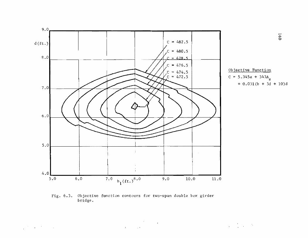
9.0r---------T---------T---------T---------~--------~------~
d(ft.) c = 482.5
8.0~ __ ------~--------.... ~~--------+_-~----~~~~~~~~--------~
5.0~--------~-------- __ +_--------~----------+_--------_+----------~
4.0~ ______ ~ ________ ~ ________ ~ ______ ~~ ______ ~ ________ ~
5.0 6.0 9.0 10.0 11.0
Fig. 6.3. Objective function contours for two-span double box girder bridge.
Objective Function
C = 5.345a + 343A s
+ 0.03l(b + 3d + 10)d
function is less than 0.5 percent. Examination of the contour plot
reveals that the gradient of the objective function is quite flat near
the optimum. Consequently, the optimal point is not sharply defined.
The best solutions to both problems were obtained using the
NeIder-Mead method. In the case of the Powell method, some starting
points were tried that did not lead to a solution at all. The reason
161
for this was that in one of the early iterations the method would arrive
at a point having a value of b3
or d so small that the objective function
subroutine could not obtain a value for t3' On the other hand, with the
NeIder-Mead method, the computer output always revealed a slow but steady
convergence.
The value of bl
(the width of the cantilever portion of the deck
slab) has a value of 8.00 ft. at the optimum in both problems. The
apparen t reason for this "round figure" value is tha t for grea ter wid ths
a second wheel load would be acting on the cantilever, giving a discon
tinuity in the gradient of the objective function at this value. The
value of b2 (the width of the outer interior span of the deck slab) is
such that this span is less than the central span, bs ' The value of b3 (the width of the lower slab) is such as to give sloping webs for the box
girders.
The effect of increasing the unit cost of the cables as done in
the second problem is to increase the value of the depth d at the optimum
and to decrease the value of b3
. The increase in d was expected because
the required cable area decreases with the depth of the superstructure.
Optimal LId ratios decreased from 29 to 25 with increased tendon costs.
The bottom flange area required for negative moment also decreases with the
depth; hence the decrease in b3
.
The contour plot for the first problem (Fig. 6.3) shows that the
objective function is not very sensitive to small changes in the variables
near the optimal point. In other words, as already noted, the gradient is
flat. A range of values of bl
and d to give values of the objective
function within 1 percent and 2 percent of the optimal value are as follows:

162
Objective Function Range of b1 (ft) Range of d(ft) Range of Lid
1 percent above optimal value 6.8 to 9.0 5.6 to 7.1 32 to 25
2 percent above optimal value 5.3 to 10.8 5.2 to 7.7 35 to 23
6.4 Second Examp1e--Two-Span, Multi-cell Box Girder Bridge
The cross section of the second example bridge to be optimized is
shown in Fig. 6.4. The spans, the support system, and the cable pattern
are the same as for the first example. The constants and the variables
for the nonlinear programming problem are the same as in the previous
example, apart from the following exceptions to the constants.
The dimension b6
does not appear in this example. The following
item is added:
n number of webs w
Four webs are shown in Fig. 6.4. However, the subroutine is set up to
handle any arbitrary number. If there are more than four webs, the
interior spans of the deck slab, apart from those adjacent to the canti
lever portion, are all set equal to bS
'
The procedure for computing the objective function is similar to
that used in the previous case. A listing of the subroutine is given in
Appendix C.4. The constants b, t 4 , and nw are set to the following values:
b 50
t4 1.0833
n 4 w
Two problems are again conSidered, corresponding to two values of
cable cost. As before, the objective functions are given by:
First problem:
Second problem:
C 5.345a + 343A + 0.03l(b + 3d + 10)d s
C = S.34Sa + 5l4.SA + 0.03l(b + 3d + 10)d s
The optimal solutions obtained from the Ne1der-Mead method and the
Powell method are shown in Table 6.2.
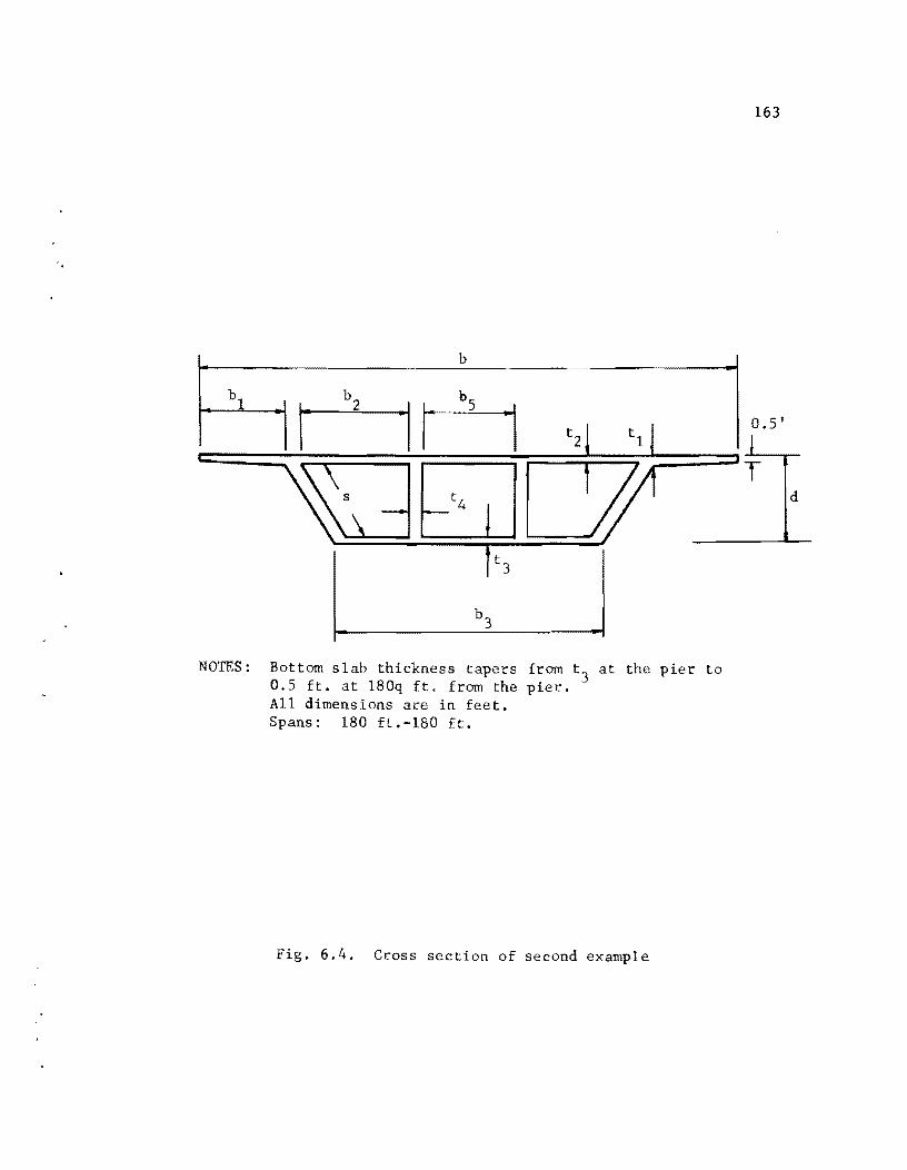
'.
b
b b2
'I~ r t2
Q t3
NOTES: Bottom slab thickness tapers from t3 at the pier to 0.5 ft. at l80q ft. from the pier. All dimensions are in feet. Spans: 180 ft.-180 ft.
Fig. 6.4. Cross section of second example
163
0.5'
T d

TABLE 6.2. OPTIMAL SOLUTION FOR TWO-SPAN THREE-CELL BOX GIRDER BRIDGE
Method Starting Point Solution
Variab 1es (feet) Variables (feet) Objective Function
b 1 b2 b3 d b 1 b2 b 3 d Lid ($ per ft.)
Objective function: C = 5.345a + 343A + 0.031 (b + 3d + 10)d s
NeIder-Mead 6.0 10 .0 20.0 8.0 10.83 6.46 24.39 5.95 30.2 509.63
Powell 6.0 10.0 20.0 8.0 11.00 6.29 24.39 5.91 30.4 509.68
Best Solution 10.83 6.46 24.39 5.95 30.2 509.63
Objective func t ior,: C = 5.345a + S14.5A + 0.031(b + 3d + 10)d s
NeIder-Mead 6.0 10.0 20.0 8.0 10.89 6.10 23.25 6.32 28.5 582.45
Powell 6.0 10.0 20.0 8.0 14.30 8.12 17.28 6.83 26.3 581.20
Powell 10.0 8.0 20.0 8.0 13.78 7.68 18.30 6.69 26.9 581.28
Best Solution 14.30 8.12 17.28 6.83 26.4 581.20

165
A contour plot for the first problem is given in Fig. 6.5. The
axes correspond to the variables bl
and d. As in Sec. 6.3.3, the
variables b2
and b3
are expressed in terms of bl
in such a way that the
correct values are obtained at the optimal point; thus,
b2 = 0.269(b - 2b l - 4t4 )
b3 = 0.86l(b 2b l )
6.4.1 Comments on the Optimal Solution. As in the previous
example, there is some variation in the values of the variables at the
optimal point, obtained with the different methods and different starting
points. The variation in the optimal value of the objective function does
not exceed 0.2 percent. Again, the flat gradient of this function is the
reason why the optimal point is not sharply defined.
The best solution for the first problem was obtained by the
NeIder-Mead method and for the second problem by the Powell method. The
Powell method yielded solutions with all of the starting points tried.
In view of the small variation in the solution values of the objective
function, the two methods can be considered about equally effective in
this example.
The values of bl
and b3
in the optimal solutions indicate a large
cantilever overhang for the top slab and a narrow bottom slab. The
apparent reason for this is that a large area of bottom slab is required
only in the negative moment region near the pier, thus leading to a narrow
width for the optimum, and in consequence the cantilever portion of the
top slab becomes large, avoiding excessive slopeof the outside webs.
The effect of increasing the unit cost of the cables is again to
increase the value of the depth d at the optimum. Lid decreases from 30
to 26 with increasing tendon costs. Also the value of b3
decreases and
that of bl
increases.
The contour plot for the first problem (Fig. 6.5) again indicates
that the objective function is not very sensitive to changes in the
variables near the optimal point. The range of values of b l and d giving
values of the objective function within 1 percent and 2 percent of the
optimal value are as follows.

9.0~------~--------~--------~------~~------~--------~
d (ft. )
8.0~--------4---------~---------+--------~~~~~n-+---------~
6.0~-----.~~~~~-4+-.r--~~+-~~----+-------~+-----~--~
4.0L-______ ~ ________ ~ ________ ~ ________ ~ ______ ~ ________ ~
8.0 9.0 10.0 13.0 14.0
Fig. 6.5. Objective function contours for two-span three-cell box girder bridge

Objective Function
1 percent above optimal value
2 percent above optimal value
6.5 The Optimal Solution as a Basis for Design
Range of bl (ft)
9.8 to 13.7
8.8 to >14.0
167
Range of d (ft) Range of L/d
5.3 to 6.6 34 to 27
4.9 to -7.2 36 to 25
The procedure developed in this chapter makes possible the deter
mination of the optimal basic dimensions (bl
, b2
, b3
, and d) for the cross
section of a two-span bridge, of given length, width, and sectional type.
These optimal dimensions can form the basis for the design of the bridge.
As noted in Chapter 2 and Sec. 3.8, the first step in the design
of the superstructure is to select an approximate cross section. The
full dimensions, including the various thicknesses, are required. These
latter dimensions, classified as dependent dimensions in Sec. 6.1, may be
otained as follows.
The subroutine developed to compute the objective function can
easily be converted into a program to compute the full dimensions of the
section. The variables bl
, b2
, b3
, and d can be made input items for
this program and the various dimensions computed by the subroutine, e.g.,
the slab thicknesses, the section area, and the cable area, can be printed
as output. Thus, this program performs the function of a preliminary design.
6.6 Possible Limitations of the Optimal Solution
The question must finally be raised as to whether the cross section
determined by the optimal solution, i.e., having the minimum cost, is in
fact the most appropriate one to use in design. The following considera
tions are relevant.
The op timal d ep th, d, obtained using the bes t es tima te of cable
cost, came to 6.30 ft. in the case of the double box girder and 5.95 ft.
for the three-cell box girder. These correspond to a span/depth ratio of
about 30, which is higher than that for most box girder bridges actually
constructed abroad. It is to be noted that the smaller the depth the
greater the number and the crowding of the cables. However, there is no

168
reason to consider this excessive for these values of d. The higher
span/depth ratios may be reflecting both lighter U.S. live loads and
different economic conditions.
Deflections are also greater for smaller depth. A deflection
limitation was not built into the subroutine for the objective function.
This could be done but would add significantly to the complexity. In
view of the very small deflections obtained for the bridge designed in
Chapter 3 and considering that the dead load was balanced, it is unlikely
that the deflections obtained for the optimal values of depth, given
above, will be excessive.
In the case of the three-cell box girder, the optimal values of
b1
indicate a large cantilever overhang. The larger the overhang the
more crowded the transverse reinforcement becomes in the top of the slab.
It is also possible that with a large value of bl
the shear stresses in
the outer webs of the girder may be considerably higher than those in
the inner webs. A large inequality of shears will probably result in a
greater quantity of web reinforcement being required.
The flat gradient of the objective function near the optimum allows
a reasonable latitude in the choice of the dimensions without large varia
tion in this function. So an increase in depth or a decrease in the
cantilever overhang (in the case of the three-cell box) can be made with
small increase in cost.
6.7 Other Examples for Optimization
The methods developed in this chapter for optimizing two-span
bridges can be extended to bridges having a greater number of spans.
The changes in procedure will follow the changes outlined in the design
method.
In the case of long viaducts, the span could also be made a
variable to be optimized. This will be discussed further in the next
chapter.

C HAP T E R 7
OPTIMIZATION OF BRIDGES CONSTRUCTED IN CANTILEVER
The problem of optimizing the cross section of bridges constructed
in cantilever will be considered in this chapter. The difference in the
design procedure for a bridge of this type as compared to one constructed
on falsework will be reflected in the subroutine to compute the objective
function for the problem. Otherwise, the optimization procedure is essen
tially similar to that described in the preceding chapter and the basic
steps are as follows;
(a) A mathematical model of the structure is set up.
(b) A subroutine is developed to calculate the objective function.
(c) The nonlinear programming problem is solved using the NeIder-Mead method and/or the Powell method.
The sample case for which the optimization is carried out in full
is that of a three-span bridge, having the same length and span ratio as
that designed in Chapter 4. The function to be minimized will again be
the cost of the bridge. The method used in this example can be readily
extended to other lengths of bridge. Extension of the method to bridges
with other span ratios and to viaducts having many spans will be discussed.
7.1 Example Case--Three-Span Double Box Girder Bridge
The cross section of the example bridge is shown in Fig. 7.1. It
consists of a pair of connected, single-cell box girders. The segmental
pattern, the cable pattern and the support system are the same as for
the bridge designed in Chapter 4. The spans are 100 ft. - 200 ft. -
100 ft.
The constants, independent variables, and dependent variables for
the nonlinear programming problem are the same as in Sec. 6.1. The
169

170
NOTES: Bottom slab thickness varies from t3 at main pier to 0.5 ft. at 100q ft. from pier. All dimensions are in feet. Spans: 100 ft.-200 ft.-lOO ft.
Fig. 7.1. Cross section of example for cantilever erection
.-

171
objective function C, the cost of the bridge per foot length, is a function
of the independent variables; thus
The problem will again be treated as unconstrained.
7.2 The Objective Function
The subroutine given in Appendix C.S is developed to calculate
the objective function, by performing an approximate design of the super
structure and summing the costs of the various components.
The basic steps adopted in the approximate design are as follows:
(a) The deck is designed for wheel loads.
(b) The bottom slab thickness and the top cables are designed for cantilever erection.
(c) The bottom cables are designed for ultimate load on the completed superstructure.
This procedure closely follows that outlined in Chapter 4, except
that some steps are omitted. Various simplifications are made to
facilitate the design. These include the ones outlined in Sec. 6.2.
The material properties assumed are as given in Chapter 3.
7.2.1 Design of Deck. This is exactly the same as in Sec. 6.2.1.
7.2.2 Properties of Concrete Section at Center of Bridge. The
following properties of the minimum section are next computed by the
subroutine.
all area of ~e half section (i.e., one .box girder)
a l = area of ~e full section
d cl
~ distance from top of girder to centroid of ~e half section
7.2.3 Bottom Slab Thickness. The bottom slab thickness at the
main piers, t3
, is designed to give adequate compressive capacity for
ultimate strength during cantilever erection. The ultimate load factors
are the same as in Sec. 3.6. The approximate bending moments are calcu
lated as in Sec. 4.7.2 and the ultimate moment is as follows for each box
girder.

172
M = 1.35(Dead load moment) + 2.25(Live load moment) u 2
1.35(0.150a ll X 100 /2) + 2.25(25 X 95)
1012.5all
+ 5,344
The distance from the top of the girder to the center of the top
cables is assumed to be 0.46 ft., as in the bridge designed in Chapter 4.
Moment arm: dm
= d - 0.46 - 0.5t3
The required value of the thickness is given by
t3 = M)(dm X q'l X 0.85f'c X b3)
_. M /(d . X 0.9 X 0.85 X 6 X 144 X b3
) u n,
M /(661 d b3
) u m
The value of q, the fraction of the cantilever span over which the
bottom slab must be thickened, is now calculated. At the end of the taper
the bottom slab thickness is 0.5 ft. and the ultimate moment capacity is
obtained as follows.
Moment arm: d m
d - 0.46 - 0.5(0.5)
-d-O.71
Moment capacity: Mu(min) = dm X ~ X 0.85f~ X b3 X 0.5
dm X 0.9 X 0.85 X 6 X 144 X b3 X 0.5
The actual ultimate moment at a distance (lOOz) ft. from the pier
center is given by
M (z) u
1.35(DL moment) + (LL moment)
1.35 X 0.5 X 0.150all [lOO(1 -
2.25 X 25(95 - 100z) 2
1012.5all (1 - z) + 5,625(0.95
2 z)] +
- z)
The subroutine computes the value of M (z) for successive values u
of z, starting from z = 0.10 until a value less than M (min) is obtained. u
The fraction q is set equal to the value of z at that point.
7.2.4 Properties of Concrete Section at Main Piers. The following
properties of the maximum section can now be computed by the subroutine.

a21
:::: area of the half section
a2 = area of the full section
dc2 :::; distance from top of girder to centroid of the
half section
7.2.5 Top Cable Area. The top cables are designed to balance
60 percent of the dead load during cantilever erection.
The moment to be balanced at the pier for each box girder
(i.e., the half section) is given by
M = 0.6(Dead load moment) 2 = 0.6 X 0.150a ll X 100 /2
= 450an The eccentricity of the cables about the section centroid is
d = d - 0.46 ec c2
The effective prestress: f = 0.6f' = 162 ksi se s
The top cable area required for the full cross section at the
pier is given by
Asl = 2 X M/(d ec X fse)
= 2 X 450a11 /(d ec X 162 )( 144)
:::: 0.0386a l1/(d c2 - 0.46)
173
The capacity of the cables at ultimate load is now checked. From
Sec. 7.2.3 the ultimate moment at the pier is given by
Mu ~ 1012.5all + 5,344
and the moment arm is
dm = d - 0.46 - 0.5t3
The following (conservative) value is assumed for the cable stress at
u1 tima te load
f - 240 ksi su
Hence, the top cable area required for ultimate strength is .given by
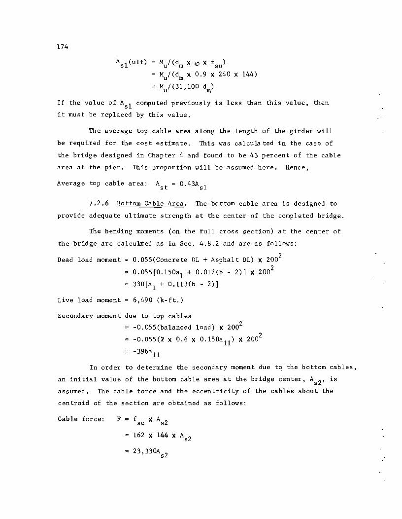
174
Mu/(dm X W X fsu)
M /(d X 0.9 X 240 X 144) u m M /(31,100 d ) u m
If the value of Asl computed previously is less than this value, then
it must be replaced by this value.
The average top cable area along the length of the girder will
be required for the cost estimate. This was calcuffited in the case of
the bridge designed in Chapter 4 and found to be 43 percent of the cable
area at the pier. This proportion will be assumed here. Hence,
Average top cable area: Ast = 0.43Asl
7.2.6 Bottom Cable Area. The bottom cable area is designed to
provide adequate ultimate strength at the center of the completed bridge.
The bending moments (on the full cross section) at the center of
the bridge are calcu~ed as in Sec. 4.8.2 and are as follows:
Dead load moment
Live load moment
0.055(Concrete DL + Asphalt DL) X 2002
0.055fO.150al + 0.017(b - 2)] X 2002
330[a l + 0.113(b - 2)]
6,490 (k-ft.)
Secondary moment due to top cables
-0.055(balanced load) X 2002
-0.055(2 X 0.6 X 0.150a ll ) X 2002
= -396all
In order to determine the secondary moment due to the bottom cables,
an initial value of the bottom cable area at the bridge center, As2 ' is
assumed. The cable force and the eccentricity of the cables about the
centroid of the section are obtained as follows:
Cable force: F = f X A se s2
- 162 X 144 X As2
= 23,330As2

The distance from the bottom of the girder to the center of the bottom
cables is assumed (conservatively) to be 0.5 ft.
Cable eccentricity: dec = (d - dcl 0.5)
175
Since the cable pattern and segmental pattern are the same as in
Chapter 4 the equivalent cable load and the secondary moment may be
obtained in the same way as in Sec. 4.8.4. The equivalent load for the
main span bottom cables is given by
P F X d 1(6 X 10) ec 23,330A 2d 160
s ec 388.8A 2d s ec
The secondary moment due to the main span bottom cables is (0.1013 X
P X 200). In Chapter 4 the secondary moment due to the side span bottom
cables amount to 14 percent of this value, So it is assumed here that
the secondary moment due to all of the bottom cables is given by
MS 1.14 X 0.1013 X P X 200
1.14 X 0.1013 X 388.8A 2d X 200 s ec
= 8,980A 2d s ec
The ultimate moment at the center of the bridge can now be
determined; thus
M 1.35(DL moment) + 2.25(LL + Impact moment) u
+ (Secondary moments)
1.35[330(al
+ O.113(b - 2» + 2.25(1.154)(6,490)
+ (-396a ll + MS)]
445.5[a l + 0.113(b - 2)] + 16;850 - 396a ll + MS
The required cable area is now determined. In Sec. 4.8.4 a value
of 267.5 ksi was calculated for the cable stress at ultimate load at the
bridge center. The following conservative value will be assumed here.
f su
Depth of stress block:
= 265 ksi
d -A2f 1(0.85fb) a s su c
As2 X 265/(0.85 ~ 6 X b)
== 52A s2 / b

176
Moment arm: d m
d - 0.5 - 0.5d a
d - 0.5 - 26A s2 /b
Bottom cable area required at center of bridge:
= M / (d X (I') X f ) u m su M /(d X 0.9 X 265 X 144) u m
= M / (34, 340d ) u m
The subroutine thus computes the correct value of As2 by an
iterative procedure, starting with the assumed value.
The average bottom cable area over the full length of the bridge
was calculated in the case of the bridge designed in Chapter 4 and found
to be 47.5 percent of the area at the center. The same proportion will
be assumed in this calculation.
Average bottom cable area: Asb = 0.475As2
7.2.7 Average Section Area and Cable Area. The average cross
sectional area is
The average area of top and bottom cables is
A s
7.2.8 Cost per Foot Length of Bridge. The unit costs fur this
bridge are the same as in Sec. 6.2.7. However, earth fill is not consid
ered in this case, as it is assumed that a conventional short span struc
ture leads up to each end pier of the bridge (as in Chapter 4) rather than
an earth embankment.
The objective function, i.e., the total cost per foot length, is
given by the same expression as in Sec. 6.2.8, except that the last term
(corresponding to earth fill) is dropped. Thus,
C = 5.345a + 343A s
A listing of the subroutine that computes the objective function,
C, is given in Appendix C.5. The constants b, b6
, and t4 are set to the
following values corresponding to the design in Chapter 4.

7.3 The Optimal Solution
b 56.0
b6
= 2.0
t4 1.0
The nonlinear programming problem having the above objective
function was again solved using both the NeIder-Mead method and the
Powell method.
A second problem was also solved in which the cable cost was
increased by 50 percent. The objective functions for the two problems
are as follows:
First problem: C
Second problem: C
5.345a + 343A s
5.345a + 5l4.5A s
The solutions obtained are shown in Table 7.1.
177
A contour plot obtained by computer for the first problem is
presented in Fig. 7.2. The axes correspond to the variables b l and d.
As in Sec. 6.3.3, the variables b2
and b3
are expressed in terms of b l in such a way that the correct values are obtained at the optimal point;
thus
b2 0.322(b - 2b l - 4t4 )
b3
0.783(b2 + 2t4
)
7.3.1 Comments. As in the examples of the previous chapter,
there is some variation in the values of the variables at the optimal
point, obtained with different methods and different starting points.
The flat gradient of the objective function is again the reason for this.
The variation in the optimal value does not exceed 0.2 percent.
The best solution to both problems was obtained by the Nelder
Mead method. As in the first example of the previous chapter, the
Powell method failed to give a solution for some starting points that
were tried.
The geometry of the cross section defined by the optimal solution
for each problem is similar to that obtained in the first example of

TABLE 7.1. OPTIMAL SOLUTION FOR THREE-SPAN DOUBLE BOX GIRDER BRIDGE
Method Starting Point Solution
Variables (feet) Variables (feet) Objective Function
b1 b2
b3 d b
1 b2 b3
d Lid ($ per ft.)
Objective function: C '" 5.345a + 343A s
NeIder-Mead 6.0 10.0 10.0 8.0 8.00 11.62 10.14 5.72 34.9 463.64
NeIder-Mead 6.0 10.0 5.0 8.0 8.00 11.60 10.65 6.l3 32.6 463.62
Powell 10.0 8.0 7.0 5.0 8.00 11.61 10.07 5.76 34.7 463.66
Best Solution 8.00 11.60 10.65 6.l3 32.6 463.62
Objective function: C = 5.345a + 514. 5A s
NeIder-Mead 6.0 10.0 10.0 8.0 8.00 11.54 9.76 6.78 29.5 521.79
NeIder-Mead 6.0 10.0 5.0 8.0 8.00 11.54 9.32 6.75 29.6 522.71
Powell 10.0 8.0 7.0 5.0 8.00 11. 53 9.08 6.86 29.2 522.75
Best Solution 8.00 11.54 9.76 6.78 29.5 521.79
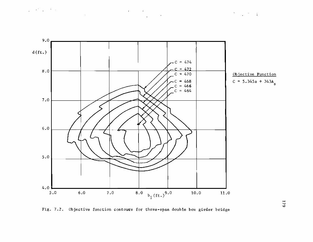
9.0r---------r-------~--------~--------~--------~--------_.
d(ft.)
474
8.0~--------+---------+---------~------~~~~~~~--------,
= 468 466 464
7.0~--------4---~~--~~--~~~~~~~~r_--------~--------__i
4.0 ~ ________ ~ ________ ~ ______ ~ ________ ~ ________ ~ ________ ~
5.0 6.0 7.0 8.0 10.0 11.0
Fig. 7.2. Objective function contours for three-span double box girder bridge
Objective Function
C = 5.345a + 343A s

180
Chapter 6. The value of b l (the width of the cantilever portion of the
deck) has a "round figure" value of 8.00 ft. The value of b2
(the width
of the outer interior span of the deck slab) is such that this span is
slightly less than the central span, b5
. The value of b3
(the width of
the lower slab) is such as to ensure sloping webs for the box girders.
The effect of increasing the unit cost of the cables is again
to increase the value of the depth d at the optimal point. The value
of b3
decreases also as before.
The contour plot for the first problem (Fig. 7.2) again indicates
that the objective function is not very sensitive to changes in the
variables near the optimal point. It may also be noted that the contours
are more irregular than in the previous cases. The range of values of b l and d to give values of the objective function within 1 percent and 2 per
cent of the optimal value are as follows.
Objective Function Range of bl(ft) Range of d(ft) Range of L/d
1 percent above optimal value 6.8 to 8.7 5.1 to 6.8 39 to 29
2 percent above optimal value 5.6 to 9.8 4.6 to 7.5 43 to 26
7.3.2 Possible Limitations of the Solution. The optimal depth d,
obtained in the first problem (i.e., using the lower value of cable
cost) is 6.1 ft. This corresponds to a span/depth ratio of 33, which is
higher than that occurring in any of the existing bridges recorded in
Ref. 16 except for those having variable depth. So the question arises
as to whether or not the optimal depth should be used for design in this
case.
First, deflections must be considered. As in the previous chapter,
no deflection limitation was built into the subroutine for the objective
function. However, a rough estimate of the deflection at the center of
the bridge can be obtained by a comparison with the bridge designed in
Chapter 4. The maximum dead and live load deflection (excluding creep
effects) in that case was 0.88 in. Assuming that the deflection is
inversely proportional to the square of the box girder depth, the approxi
mate deflection in the present case is 0.88 X (8.0/6.1)2 = 1.52 in. = span/1600. This is quite acceptable.

181
The size of the top and bottom cables required will be roughly
inversely proportional to the depth of the girder. With larger cables
bigger fillets may be required to provide adequate concrete cover. Fillets
were ignored in the optimization process, as noted in Sec. 6.2, and it
is considered that they would not significantly affect the optimum depth.
The girder section corresponding to the optimal solution is the
one having minimum cost. However, in view of the flat gradient of the
objective function, a design having some improved features, namely
smaller deflections and smaller cable and fillet sizes, can be obtained
at small increase in cost by increasing the depth above the optimal. The
actual value used in construction of the example bridge (Lid = 25) is
near the 2 percent above optimal limit. This bridge was so stiff that
higher Lid ra tios seem ind ica ted.
7.4 Effectiveness of the Optimization Techniques
The following is a summary of the previous comments regarding
the effectiveness of the optimization techniques:
(a) Treatment as an Unconstrained Problem.--In each of the three
examples considered, the problem of optimizing the dimensions of the
bridge cross section was set up as an unconstrained nonlinear programming
problem. The cost per foot length was chosen as the objective function
and expressed in terms of the basic variables, bl
, b2
, b3
, and d.
Physically acceptable solutions were obtained for these variables in all
cases, thereby justifying the treatment as an unconstrained problem.
(b) The NeIder-Mead and Powell Methods of Optimization.--Calcula
tion of derivatives of the objective function was not feasible. The
NeIder-Mead and the Powell methods were accordingly chosen, being the
most efficient of the methods that do not require derivatives. In the
examples considered, the NeIder-Mead method was generally superior to the
Powell method. In two of the three examples, with some starting points
the Powell method would not reach a solution. With the NeIder-Mead method
steady convergence to the solution was always attained.

182
(c) Design Simplifications.--In calculating the objective function
an approximate design of the superstructure was carried out by the sub
routine. Various simplifications were made in this design, as outlined
in Sec. 6.2. It was considered that these would have little effect on
the solution value of the basic variables at the optimal point.
(d) Contours of the Objective Function.--Two-dimensional plots of
contours of the objective function were obtained by computer for each of
the three examples. In each case the plot showed that the gradient of
the objective function near the optimal point was quite flat. Variations
in the values of the variables bl
and d over a considerable range produce
only small changes in the value of the objective function.
(e) Effect of Changes in Unit Costs.--By varying the cost of the
cables by 50 percent, it was found that the optimal point is sensitive to
relative changes in the unit costs. A 50 percent increase in cable cost
causes an increase of about 1 ft. in the optimal value of d. The value
of b3
decreases.
(f) Deflections.--No deflection limitation was built into the
objective function subroutines. Approximate estimates indicate that for
the examples considered deflection is not critical. However, if bridges
with much greater spans were being optimized, it would be best to have a
deflection limitation in the subroutines.
(g) Design Dimensions.--The optimal solution defines the basic
dimensions of the cross section for the bridge having minimum cost.
However, by utilizing the flat gradient of the objective function, the
design dimensions can be varied to some extent with only.small increase in
cost. An increase in the depth d will result in smaller deflections and
also fewer or smaller cables. In the case of a multi-cell girder, a
decrease in the cantilever overhang bl
will result in less crowding of the
transverse reinforcement and a better distribution of shears.
7.5 Other Examples for Optimization
The optimization of other cases of bridges constructed in canti
lever will now be considered briefly.

183
7.5.1 Multi-Cell Box Girder. The procedure for a multi-cell box
girder bridge is similar to that for the example considered in this chap
ter. Some minor changes are required in the objective function subroutine,
as was the case for the second example in Chapter 6.
7.5.2 Side Span Greater than Half Main Span. In the case of a
three-span bridge in which the span lengths are specified, the optimiza
tion process can be generally similar to that used in the example of this
chapter. However, when the side span is greater than half the main span,
the design procedure and the calculation of the objective function will
be a little more complex.
More generally the different spans will not be specified but only
the total length of the bridge. The side span can be made one of the
independent variables to be optimized. An alternative case is that of a
bridge crossing a navigation canal, where the main span is specified and
the side span can be a variable. The two cases can be treated in essen
tially the same way. They differ from the problems already considered in
that there is an extra variable, the side span length.
In Sec. 4.10.4 it was pointed out that when the side span exceeds
half the main span, the final outer portion of the superstructure cannot
readily be erected by the cantilever process and that some fa1sework will
normally be required. The amount of this falsework will depend on the
length of the side span in excess of half the main span. Its cost must
be included in the objective function, when the side span is a variable.
7.5.3 Continuous Viaducts. With continuous viaducts, comprising
many spans, the span length should be included among the independent
variables in the optimization problem. The number of piers will depend
on the span and so the pier and bearing costs must be included in the
objective function.

!!!!!!!!!!!!!!!!!!!"#$%!&'()!*)&+',)%!'-!$-.)-.$/-'++0!1+'-2!&'()!$-!.#)!/*$($-'+3!
44!5"6!7$1*'*0!8$($.$9'.$/-!")':!

C HAP T E R 8
CONCLUSIONS
8.1 General Conclusions
The prestressed concrete box girder constitutes an effective and
economical member for the superstructure of a long span bridge. Segmental
precasting provides an economical means of manufacture, with high quality
control, and leads to rapid methods of erection. A number of long span
bridges have been constructed throughout the world using segmental precast
box girders and techniques of precasting and jointing are available for
high strength and precision.
There are two principal methods of construction, namely erection
on falsework and cantilever erection. The former is generally simpler
provided support for the falsework is feasible at fairly close intervals.
Cantilever erection is usually more suitable for river crossings and for
viaducts over water or heavily traveled roadways.
Procedures for the design of such bridges erected on falsework or
erected in cantilever have been developed. These procedures involve using
"beam" theory analysis procedures to satisfy both service load criteria
and ultimate strength criteria under all conditions of loading. The
effect of the cable forces on the concrete stresses is calculated using
an equivalent load concept. Service load level stresses considering
possible warping effects and effects of unsymmetrical loading throughout
the structure are then checked using the MUPDI program developed by
A. Scordelis. Erection stresses in bridges erected in cantilever are
also checked using the SIMPLA2 program developed by R. Brown.
For bridges erected on falsework, the prestressing system can con
sist of long, draped cables. If the number of spans is small, these can
run the full length of the bridge and are inserted and tensioned at the
end of construction. A cable profile consisting of a series of parabolas
185

186
will produce a series of uniform equivalent loads along the girder. The
cables and the concrete section must provide adequate ultimate strength
and acceptable service load stresses under dead load and the various
live load patterns on the continuous superstructure.
In the case of bridges erected in cantilever, each stage of
construction is a separate design condition, for which the ultimate
strength and service load criteria must be satisfied. The cables are of
varying length. Those in the top of the girder are inserted and ten
sioned as each pair of segments is erected and must withstand the dead
load and possible unbalanced moments in the cantilever arm. The cables
in the bottom of the girder are inserted after completion of the canti
lever arms and casting of the closure and are designed to ensure adequate
ultimate strength and satisfactory service load stresses under dead and
live load on the completed bridge. To obtain the effect of the cable
forces on the concrete stresses, the equivalent load concept has been
further developed for application to a system of cables of varying
length.
Mathematical methods of optimization have been adapted to the
problem of finding the optimal cross sections, i.e., those having minimum
cost, for bridges constructed on falsework and bridges erected in canti
lever. Two types of cross section were considered--a pair of connected
single-cell box girders and a multi-cell box girder. In each case the
problem was treated as an unconstrained nonlinear programming problem in
four variables that define the geometry of the cross section. A subroutine
was developed to compute the objective function, taken as the relative
cost of the bridge per foot length, and a solution obtairied by the
NeIder-Mead method and the Powell method.
The optimal solution obtained for each problem defines the basic
dimensions of a cross section having minimum cost. However, to some
extent the dimensions can be varied with small increase in cost, because
it was found from two-dimensional contour plots that the gradient of the
objective function is quite flat near the optimum. The range of variation
of the variables for a given increase in cost can be readily obtained
from the contour plots.

187
The dimensions of the section for minimum cost are sensitive to
relative changes in the unit costs of the materials. An increase in
the cost of the cables, for example, causes an increase in the optimal
depth. Studies using the optimization programs were limited to the gen
eral spans and roadway widths of the example problems. Results should
not be widely generalized until further parameter studies are made.
8.2 Particular Conclusions
The following conclusions apply to the particular examples treated
in Chapters 3, 4, 6, and 7, and may not necessarily apply to other cases,
such as bridges with different spans, widths, and loadings.
For the bridges designed in Chapters 3 and 4, the more accurate
stress analyses obtained with the MUPOI and SIMPLA2 programs confirmed
the adequacy of the basically simple design procedures adopted. These
procedures utilized hand calculations and beam theory to determine the
basic concrete section and the layout and size of the prestressing cables
required.
In the case of the bridge constructed on falsework (Chapter 3),
the cable profile consisted of three parabolas and the equivalent cable
loads were determined accurately. However, in the case of the bridge
erected by the cantilever method (Chapter 4), the design procedure
utilized approximate estimates of the equivalent loads of the system of
cables. This procedure resulted in a satisfactory design, as confirmed
by the MUPDI and SIMPLA2 analysis.
In the design of the bridge constructed on falsework, full length
draped cables were adopted and their size determined by a simple load
balancing procedure. The cable area was set equal to that required to
balance the dead load, assuming an idealized, double-parabolic profile
for this purpose. The area so determined gave satisfactory service load
stresses and ultimate strength.
For the bridge constructed by the cantilever method, it was found
that the top cables could be designed to balance a uniform load of about
60 percent of the dead load on the completed cantilever. The quantity of
188
cables so determined gave acceptable service load stresses and adequate
ultimate strength during construction. The MUPDI program was used to
determine a suitable pattern for the bottom cables. These were designed
to give adequate ultimate strength under live load on the completed bridge
and their quantity was adjusted after analysis to give better service
load stresses.
Stress distributions obtained by the MUPDI analyses for both
bridges designed indicated a variation of stress across the sections at
the main piers, because of shear lag, and an almost uniform stress dis
tribution across the top and bottom slabs at sections of zero shear.
Studies in Chapters 6 and 7 showed that the problem of optimizing
the cross section of the bridge could be treated successfully as an uncon
strained nonlinear programming problem. Physically acceptable solutions
were obtained in all cases.
Of the two optimization methods used, the NeIder-Mead method was
generally the more effective. It always gave steady convergence to a
solution. On the other hand, in two of the three examples considered,
the Powell method did not reach a solution for some starting points. The
NeIder-Mead method is also the simpler of the two methods.
For sections of the double box girder type with an approximate
overall width of 56 ft., whether constructed on falsework or by the canti
lever method, the optimal width obtained for the cantilever overhang of
the deck was 8.0 ft. This is the maximum width for which there is a
single wheel load on this portion of the deck. The values of bottom slab
width were such as to give sloping webs.
In the case of the three-cell box girder, the optimal solution
indicated a large value of the cantilever overhang, a narrow bottom slab
and sloping webs. The apparent reason for this configuration being
optimal is that a large area of bottom slab is not required structurally
except in the short region of negative moment.
The span/depth ratios obtained in the optimal solutions were
approximately 30 for the two-span bridges constructed on falsework, and

189
33 for the three-span bridge constructed in cantilever. These values
are higher than those generally occurring in similar bridges, excluding
those having variable depth. The flatness of the cost gradient indicated
relatively little cost change (2%) for span/depth ratios as low as 26.
This indicates that the "optimum" ratio will be somewhat above 25 but
factors such as fillet size and tendon congestion should be considered
in selecting proportions.
8.3 Recommendations
Important design cases not considered in detail in this report
include skew bridges and bridges with variable depth. These should be
investigated more fully.
Highway crossovers will often be skewed. The design and analysis
of such bridges will require modifications to the procedures developed
for normal bridges. A few computer programs are now available for
analyzing box girder skew bridges and these could be used in the way
MUPDI was used in this study. Skew will also create some difficulties
with segmental precasting. One solution is to cast a few segments near
the ends of the span on the skew and the remaining segments normal to
the roadway axis. Much will depend on the pier location details in this
case.
Bridges having spans greater than 250 to 300 ftA generally vary
in depth from a maximum at the piers to a minimum at midspan. In this
way greater economy can be achieved. To a large extent the design proce
dure developed is applicable to bridges with variable depth. The finite
element analysis program FINPLA2, developed by Scordelis, can be used
for these bridges in place of the MUPDI analysis. Unfortunately, no pro
gram corresponding to SIMPLA2 exists for this case.
The optimization techniques should also be extended to cases where
the bridge span is a variable, as well as the cross-sectional dimensions.
Examples of such cases include three-span river crossings, in which the
total length is specified but not the span ratio, and also viaducts. A
wider study of effects of variables such as span and roadway width should

190
be undertaken using the optimization techniques to provide further
guidance for preliminary designs.

REFERENCES
1. Americqn Association of State Highway Officials, Standard Specifications for Highway Bridges, Tenth Edition, Washington, D.C., 1969.
2. American Association of State Highway Officials, Standard Specifications for Highway Bridges, Eleventh Edition, Washington, D.C., 1973.
3. ACI Committee 318, Building Code Requirements for Reinforced Concrete (ACI 318-63), American Concrete Institute, Detroit, 1963.
4. ACI Committee 318, Building Code Requirements for Reinforced Concrete (ACI 318-71), American Concrete Institute, Detroit, 1971.
5. American Institute of Steel Construction, Moments, Shears and Reactions--Continuous Highway Bridge Tables, New York, 1959.
6. Bureau of Public Roads, U.S. Department of Transportation, Strength and Serviceability Criteria, Reinforced Concrete Bridge Members, Ultimate Design, Second Edition, 1969.
7. Brown, R. C., Jr., "Computer Analysis of Segmentally Constructed Prestressed Box Girders," unpublished Ph.D. dissertation, The University of Texas at Austin, 1972.
8. Brown, R. C., Jr., Burns, N. H., and Breen, J. E., IlComputer Analysis of Segmentally Erected Precast Prestressed Box Girder Bridges," Research Report No. 121-4, Center for Highway Research, The University of Texas at Austin, November 1974.
9. Kashima, S., "Construction and Load Tests of a Segmental Precast Box Girder Bridge Model," unpublished Ph.D. dissertation, The University of Texas at Austin, 1974.
10. Kashima, S., and Breen, J. E., IlEpoxy Resins for Jointing Segmentally Constructed Prestressed Concrete Bridges, Center for Highway Research Report 121-2, The University of Texas at Austin, August 1974.
11. Kashima, S., and Breen, J. E., "Construction and Load Tests of a Segmental Precast Box Girder Bridge Model," Research Report No. 121-5, Center for Highway Research, The University of Texas at Austin, February 1975.
12. Khachaturian, N., "Service Load Design of Prestressed Concrete Beams-Part III: Continuous Beams," distributed by I11ini Union Bookstore, 1962.
191

192
13. Koretzky, H. P., and Kuo, T. H., "Letter Survey on State-of-the-Art in the U. S.A. of Segmental Concrete Box Girder Bridges," Penn DOT Publication No. 114, July 1974.
14. Lacey, G. C., "The Design and Optimization of Long Span, Segmentally Precast, Box Girder Bridges," unpublished Ph.D. dissertation, The University of Texas at Austin, December 1970.
15. Lacey, G. C., and Breen, J. E., "State of the Art--Long Span Pres tres sed Concrete Bridges of Segmental Cons truc tion," Research Report 121-1, Center for Highway Research, The University of Texas at Austin, May 1969.
16. Lacey, G. C., Breen, J. E., and Burns, N. H., "Long Span Prestressed Concrete Bridges of Segmental Construction--State of the Art," Journal of the Prestressed Concrete Institute, Vol. 16, No.5, October 1971.
17. Lin, T. Y., Design of Prestressed Concrete Structures, Second Edition, John Wiley & Sons, Inc., New York, 1963.
18. Maisel, B. 1., and Roll, F., "Methods of Analysis in Design of Concrete Box Beams with Side Cantilevers," Technical Report 42.494, Cement and Concrete Association, London, November 1974.
19. Muller, J., "Long Span Precast Prestressed Concrete Bridges Built in Cantilever," First International Symposium on Concrete Bridge Design, Special Publication No. 23, American Concrete Institute, Detroit, 1969.
20. Muller, J., "Ten Years of Experience in Precast Segmental Construction--A Special Report," Journal of the Prestressed Concrete Institute, Vol. 20, No.1, January-February 1975.
21. PCI Committee on Segmental Construction, "Recormnended Practice for Segmental Construction in Precast Concrete," Journal of the Prestressed Concrete Institute, Vol. 20, No.2, March-April 1975.
22. Rajagopa1an, K. S., "Comparison of Loads Around the World for Design of Highway Bridges," Paper SP-26-2, Second International Symposium on Concrete Bridge Design, Special Publication No. '26, American Concrete Institute, Detroit, 1971.
23. Scorde1is, A. C., "Analysis of Continuous Box Girder Bridges," SESM 67-25, Department of Civil Engineering, University of California, Berkeley, November 1967.
24. Structures Precontraintes, V Congres de 1a Federation Internationa1e de 1a Precontrainte, Paris, June 1966.
25. Swann, R. A., "A Feature Survey of Concrete Box Spine-Beam Bridges," Technical Report 42.469, Cement and Concrete Association, London, June 1972.
26. Wright, R. N., Abdel-Samad, S. R., and Robinson, A. R., "BEF Analogy of Analysis of Box Girders," Journal of the Structural Division, ASCE, Vol. 94, ST4, Proc. Paper 5394, August 1967.
27. Cohn, M. Z. (Editor), An Introduction to Structural Optimization, Solid Mechanics Division, University of Waterloo, 1969.
193
28. Curry, H., "The Method of Steepest Des'cent for Nonlinear Minimization Problems," Quarterly of Applied Mathematics, Vol. 2, 1954.
29. Fletcher, R., and Powell, M. J. D., "A Rapidly Convergent Descent Method for Minimization," The Computer Journal, Vol. 6, 1963.
30. Himmelblau, D. M., Applied Nonlinear Programming, McGraw-Hill Book Company, 1972.
31. Lasdon, L. S., "Notes on Linear, Nonlinear and Dynamic Programming," Typed notes, Division of Organizational Sciences, The University of Texas at Austin, 1965.
32. NeIder, J. A., and Mead, R., "A Simplex Method for Function Minimization," The Computer Journal, Vol. 7, No.4, January 1965.
33. Powell, M. J. D., "An Efficient Method for Finding the Minimum of a Function of Several Variables wi thou t Calculating Deriva tives," The Computer Journal, Vol. 7, No.2, July 1964.
34. Wilde, D. J., and Beightler, C. S., Foundations of Optimization, Prentice-Hall, 1967.

!!!!!!!!!!!!!!!!!!!"#$%!&'()!*)&+',)%!'-!$-.)-.$/-'++0!1+'-2!&'()!$-!.#)!/*$($-'+3!
44!5"6!7$1*'*0!8$($.$9'.$/-!")':!

A P PEN D I X A
PROTOTYPE BRIDGE PLANS
[195]

---~f:1.~~~~ :15'
LAVOUT
INTRACOASTAL :jp
CANAL BRIDGE PARK i'OAP 22 •
"" 4/JII '''JIC)I''''} Nrr
16 ~" OJ1 I ., IT

--j
HALl" IUyATION
-I"''-----.--~40··.!p!'" _
SI!!CTION I)-I)
......... -~ T'1 ,.
All quonldoes ~ QI¥ 1b"'"0I'W ~ h'll£t M"
.. 16 b" t. '0 t • c •• , .. .,Iortf Itl tdl ~h.l\
"If,,, ..... ~4tt."u toU .If .. '.1' (lIun" .. 1 ." .. ~ "'1." t, tu t, •• ,I' •. nut II' '.'tlU ... all .... ' •• ,. H. 't. '''!U .. lit',' .t. , ........ loCl~ un"lt. d ,,,Mt"$'" 11 •• 1 It I', ~'."tt'" . __ " ... .,~ .. j • t l t HI" U "'~'"'' , ..... , .. ,,~ , ........... . 11 '.11 t.\1 ""'f ..... HI '''' ...... >!.j .t Ilt 'f '1''''',l!tt! UtU .tt !toe ... IU \,' .... , ••
h,.,.. .. ............ I.U
.. I .... " .,.un \I .... ",.I~H'.' •• " 'U" ,. , .... [~,af'~c:.."Qt~.aI!CIII"CIS
l~<tt Itll "UHI'~I .. ,,," ~I u.t , •• " .. ••• '''''UI H •• ",,11, .. tt·" \.~~."I", f,Ut ."~"J to •• , ' ••• , a .. ,,~ 'po '."'M, {UI ..... _ tt" .... n ••••• , .. ,0 uU·'·t.I •• "! ., .• , 'I' .... ,., u, H".tU '~HI, U'u'\~" II .. , ,"f U" "''''_ .ot* /t"l U .. ttl "H·"~H't" IOf. 'U,I!tHI I ... ., .. , ..... n .. , If h.~, ... " h. un,.;. •• ' ..... lr ,~u .. tU .,_UI ... , .. If h .... ,t .,,,t, .• ,!, 'dill UI1 ',H'.U
Wttt .. "lHU .,,1 ••••••• , • ., ..... t .. 't .... 1,'1'" ." ~ •• a'l'f~l Il ....... 'I,. ,. H' , •• UNt •• •• ','U' ,1,,,,_., .,11 U .... t., $,I·u, '~1 .'c" ru! lUll u '.,.hl!.' I, b'. ", ........... c .... _I ..
TEXAS HIGHWAY OI:PAIITIoIf:WT SRltIGf: DIVISION
INTERIOR PIERS
20 & 21

---- Ji~ =j=::tj:±~=-=~;=Ef:=j--'bt:U6'6; : T
~~'I 4-~_'::::::"-..t---./-~~. ---!ii>l---+. tPl<rr20crlf'
I I I
~~-'= ---~""'_ .'--'r:::::i seeTIO .. b;~a:rc::a' f1br_,,_._ -A
_&
TYPICAL SI!CTION
~ , ~ .. -J.I ______ ,......J..I-T
~ SEARING Sl!AT Dey.
PLAT!! M!S • • Bpbf!P t1rIjI;;i
No~ ,:,,~,,*~/eQllQ(;:r¥~"~s ~(pOC,.,)..,.ol::w~ ~
%if.~~~~~f oet=Or.:llt::7t"1Ct:!' ... M .rl~rJ,l""'1!S:1
nQ'tIR:'T"" n ..... " .11. 'II .. I ,., ......... ,,'1 U ""ul, .. , " .......... ~ .. ,.~
-"~I ,.n'I' "'! P s_ U'" ""1 ••• 1, ",IU .... ,. ~:::::\Ilt'fl ...... , ••. II U •••• lUI ........ t I •• ,
S f',lln III ",'" '''' nil_ II •• ,.1 ... "."lln ., ," f,',. .... . .. "t,. , ... t'nl ...... "'lrIUI~ '" 10'1 ,",1' hn , ••
"'. '. II n tll~"'"'' '" I" I. ...... , ".,. (U'''n {cr.I""t,,· "'"' H'u"'l ..... IC. u ..... , I " r ,_""t, ••• ,, I II"" 1r •••• 1t
1 hI .... 'n'.' ... , I •• '"~. I!' U ~I l.t'rI ..... fU,II., .,11" ..... , ._ .. I"'~ ",,'u II II.U'• II.""" .. ", -, ';1 .... '~nr H 'I ..... ,. h!' Uf •• ,' u ......... "til"" In .. "ct" U ,>;ocr ••• ~~l
. !:;:;:i~; :i::~;;!; ::;:~: :i:;::!':::j:;: ::~; :~::::::':~: 11 •• hUU ••• , .,,*,AJI 1n ""
TEXAS M~GHWAY OEPAR:TMENT BRiOG£ OIVI"ON
PIER PETAILS
PIERS ?O-'.&l

~ I
-
'" . TYPICAL SeCTION
eLeVATION
Tho. d<I'~'Qn ... 11 ~. 0 15' lOad of ... and of ... ,.. CIOI"I+.I~." od!S.400n ...... ~ of' a -..qrr....... """ __ h .. _II 11M .,....., .. a
qu,d4 In .. _ .... o .... nq .... ..,~ aI~,...-uct"1O"l ~ 'IOC).".nq ~n:;rt ... Gti"ac.1'WCII 'to ... CG""i".,o __
':>-'<9- ........ ."or' forc<t~ ... bIP ~"-.--:I j..ro""dod ..-rq ,..".n,m,.1T) 0.-......."., (~ ~"'c.-r ........ ,... .: ... o .... on __ 1C>~ .... o.d
Tr.d.rH"I FQ~or$ 'or cG/co.JJaf''''9 ~/F~c""" pr~_f"' ••• _,If b~ Q$ 1'0110 __ '
R'9'ci Co,.,ciwi, - /teo _0002 ,.,...·.25 "~'fb'. c.-dfJ,f-/te-.ODI$ .,4. ·2.S
100:0·
~ T'jlldell SsA,ty"
h •• _ ........... , ........ , ~~ •• ,_ .. ro. ".,." .. , .. , ••• " ~ "" .. " I' ", .,'-; "~' ..... t •••. ~f II ................ U ,,,
I •• n .... ,I .... ", .. " 0'.10
t "," , .. ,.aI .. H II •. ,; •••• ",n ............ ,.·r ............. _ •. ".",., f.,., .. ....-." (' n ... c. 'tI,I'"
J " ••• I ........ tI •• ,
5,,,·.,..--,, II ........ II ,t, ..... , un' ' .... u., ............ 10 " •• , , .... It, ,.,. It It., .• , .... II", .. 'IU.U .. ,., Gt
, ... n. ,I .. "' '"~II" "'" ft, _ ... , ••• .. I. t, .... • II<' IIllt __ II .11' .IU
...... U .... : II ......
• , ...... Ju .... ·• ... ,u· .' , .. II" , II '" II ...... " I. I •• ' H~' 10' 'n" ••
"'I .bnoJi ~ ..,Itfd r'(pcf,w pnlJI#'tP.u ~ o~'rr ..tu,:,., T...--".. 4fri~~11 T.e~"'" ...... Jto.:. ..
AI ---- r.J&t' AI----I>IU· H----atJ .• -.. ----/38~· ., ----/34~· .. ----1.,·
III ~.~.
4l---~I.I· 4'---"-'!l0·"" lJ4----4'SId.0-M---W" iJ6---.JN'. 61---Nl.4" M---IotSlJ· ~----~.
MJ---ualJ' ,,"---~.,
~I¥ ..... ~
#~ b'Q.reqd".td::1r7 ~1Qpt:onal.? "'~ .c1:1~·
".,." ,."
C/ ----/rItie" a--·--I.M" CJ----_· GI----_
T[XAS HIGHWAY OEPARTMDfT BRIOGE DIVISION
PLA N AND ELEVATION
400 "T. SEGMeNTAL POST TENSIONeD UNIT
: NTBACOASTAL CANA.L
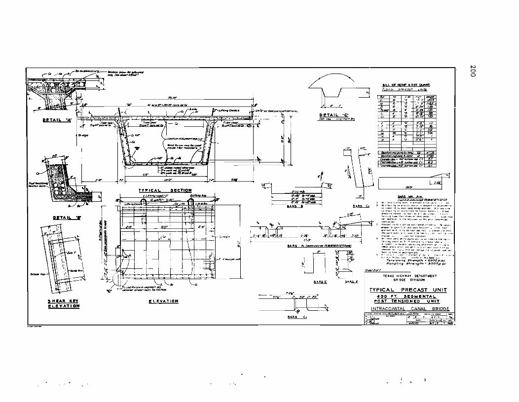
ReTAIL
""d~
SHEA" KEY ELEVATION
I
l .Jf'l.
1 l
11 I
,£
E:::::::: I. I~
iL~ 1 ~1 /-r F~
T,(~ICAL seCTION
''''''~O'' ,_ ....
,.,. 15_,,'· :J'~' -- i>fo LH>< ""'_ 1 .. ., ....
i! I I ~;~:
'I' ~O· IT r:6" 2Oe-
_r" 1_ ........, ;0- r--'
\ ---W-~_ \ --±t!-;
E
II I c~r~ ~~~-'--r"+:-~-'-- -. t--:1= -
I I
=1 , ""-,, \.. ~ /
E LEVA' ION
11"-",'6-6'"", II"-Ir &-6'''
r-----~ •
tlTAIL 'C' Aon -. /.IJ({MMM iPr
'!~n~! ~:
L--
7.0"
L---__ J_.?_._' --~---s
'ILL OF RE!NF. • Est ouyg. ',-;11::;; p.~-Catf ;.n"J
, 4 T7
'" -'!! ;;, 4
'"
... ",'.(j" 10
" 5'1. • -'5 ·c :J' 9' .>aI
-'to 7"- 5~ 0'.9' 1
'J O~6 •
.... ..,J UI 47 "'1#3) '" 4
... 6·/IoI'kMI~CI" C1 ... 8!:nHtMaiab Cr If .·0 """Cy ",
B!trItS ... 1\ AlA :';~aloIlIt.tlt1~IIJ..~IC~fj/,.u
III '''.''_f,", IU' 11""1111 •• " •• ,~ •.• H
h,., .... ~ ..... It." .. 011 ..... ,111 n ",":.":, u , ... ',,' t, "" , ••• ' .... 1"' ..... '" ' .. -"u •• ,"r''''~l I .... C ... ·~I' U _'Ii': .... ', .. f , ..
'''II''. tun. 1 ... ,ln", "; •. ,. ••. "'''' ' ..... -: I, .. , ... , H ..... '.'1 '"." •.•• ,!! ..
;:~,:::;:;., '. ,". I.! •. 'n, " " .... , ........ 1.
e 'UCI" ,-0.11 U"I nCII'.' •• ""'."" '.,.,.-, ....... ," ..... :11.,' .. 11 •• '," ••• ·• ·.,11 .,,' '"C'" .~,' " II n .. " I ••. UI • ~'"'' '-I •• " h. un'''II' .,,' ", •• ,1 I.,. ••• II' .,. .• "'1 "HI' '.: ,.IU ,~, .:~, ... ,
I '" ,:11 ·11 .. , '.'"1 'Ull .. , .~ •••••• II II. II' _. h •• ,,: "H' .. " [0 e":.11 I. "arll II ... . "':~'UL ...... 1','.11 h""1 .I." •• ~, I' ..... :0
I_H"'·'I ,',:< I", .,.! '1.", •• " ,.,. 0," eo
.Iultr a ,~" ': :"1 '" ' .... 6. '" <:r ..... 1' I.'
.... II I, .. "' .""U""" I II, :t., -. " .... :,-" rI tt,·.p .•. or
~" I.";' r, •••• , ··'."!U,' roaNU I" ren"r>f?1f?9 Sfr .... gfh • c:;OOO p ... i Haf?dfm9 Sf-rwngfM" 3000p .• ~.
TEXAS HIGHWAY DEPARTMENT BRIOGE OIVISION
TYPICAL PRECAST UNIT -400 FT. SEGMeNTAL
POST TENSIONED UNIT
I NTRACOASTAL CANAL BRIDGE
N o o

I ... .,. ~6.hnt-_*,_"
~'-1f! ~~,r~'''''~rQ!l>tt/~--
DetAIL A-A _4IfSj PRECAST UN! Mil YD
n.no
PRECAST uNIT MIl PI I'xr
rE :
seCTION D-D ~:a~fo;;,~~~~,f,
..,
I I
" ~
I
I I I
BILL OF P.EJJroF • EST QUANT PRECAST UNIT Mr •. WI.,
For "'IkIr~ VIh
BILL OF REI'" .. EST QU!,Nf. PRECAST UN" ~ pS
Jr, .n~-'" r nc .' --1;'--r-i- -e
. .# . ·4
" ." f 4 • e G, " ·4 Gz 38 ·6
-
"~",forr: r~ "
IE' II., f Z7! 5.7
r.. " /4: t5~ 14: 69 ,8: ,J!Jd
" :7 l 7 5:Y Ze5
1-
?164 58
"hftf 301 T
If> 48 ... '4 ", Z, '" /I 1?:;''1'~/n
.j .. .. ~:::;ncr 'P. cb» II
, . r~ 1:0 kI~1O
'"
TEXAS HIGHWAY DEPARTMENT BRIDGE DIVISION
//
242 '4
!:i1!-
PRECAST UNITS CS-PS·S!Q
400 PT. SEGMeNTAL POST TENSIONED UNIT
I NTRACOA5TAL CANAL BRIOOE
N o t-'

"l "-. 1
I!L.!!!YATIOH
.---..
!BCTlON A,.", SECTION a-a $I!CT!ON c-e $ECTION D-D
$ECTION e-I
5·'i<"'r:"'i4~" ____________ -I TEXAS MI6/iWAV OEPART-"ENT
BRIDGE DIVISION
TENDON PROFILES CENTER SPAN
<400 "T. SEGMENTAL. PO$T TENSIONED UNIT
I NTRACQA5TAL CAMAL _ ... , , ........... j
_ · .... T

roo
eLCYATION
seCTION H
~~ 50f7
N o UJ

ItJV qtT
5~' l'6' Z'N r.r 2·"6" l1I5' ny l!!r
........
I I ~I" I'---~ I
I , I ,
I I-r-.-I I i
~, i 01"-,}5" ....
M' 'IN' 6IJ Iar I6>t-
TENDON PROFILeS lEN)()N$ WK AI THRUM - C.I &U
TENDON PROFILes lENDONS-WI\ C3 - C.""'11
"" l"., .".' In' .,. :"., 1m-i4"
:Ir [,7.' I.!Ir \.ej-
'---
---
I,.. l :.ot- so loY r
"'"..
) hd::ns mt AlA/Clie;
.o1_ ... ..,IM l'ir ____ .lS'M
TENDON ANCHORAGe
~:~t"6&C~
~ ..
i --I--
TENDON ANCHORAGe E!lEARING. PLATE TYP£ ANC):4Qe n p ICAb DEIAIL
~,. __ ~~~_td" EM- l?1oTe'Nbtm lIe'1" N~_-----....r;L.srI' joI'k'~N
TeNDON PROFILES 1DI)QN .. " 81 & e.z
TENDON ANCHORAGe 'HEDGE TYPE ~OR ~..!:-!:. ~r, B5 i'RRu 81C
k" I - (0/' I I
TENDON P'ROflLe5 TENDONS Jr.41\.. 8.l 1HRU 61)
NO"'; .&nc:ton onchor-a~ d.'Iol/~ 0J"1II rtt;:; m"fa>~ to Irnd fypt2!S of $"rond sys1tH1"1s ~
TEXAS HIGHWAY' OEPARTMENT BRIDGE DIYISION
TENDON PROFILES AND DETAILS
400 FT, SEGMENTAL POST TENSIONED UNIT
I NTRACOAST"\L CANAL BRIDGE .... ·,·· ... • .. , ... ··"oc:noMIi'1C ~ V' ... ,_
N o ~

!lLOCKIN. DIAGRAM ~1tIIzI ., ~·~~wttII;,,,,..
SECTION THFW LONGITUDINAL .IOINT
(II"
~ = ===-=--=J ILCy. ",AHSVEASI "OINT
.. , .2Q(. 0/01.1 Ct.JI"'IC" QI'fII:II~7·.'''''''''''''0I'1::''''''
1'10,.. ""r '~.~r_,IO''''f' c;v-. I'D 0. __ lu<I.-d..., l»d prIce for ~.~f'oI Pfw,I,...s.d U'Wf"
til L OF REI'" .. EST. pen CLOSURE STAll- ,qP1o/'H'111X11J
61ZO (y J7
~7dT
TEXAS HIGHWAY O[PARTUEtH BRIDGE DIVIS_Ott
BLOCKING DETAILS
400 FT. SEGMENTAL POST TENSIONED UNIT
I NTRACOA::'TAL CANA.L BRIDGE N o Ln

!!!!!!!!!!!!!!!!!!!"#$%!&'()!*)&+',)%!'-!$-.)-.$/-'++0!1+'-2!&'()!$-!.#)!/*$($-'+3!
44!5"6!7$1*'*0!8$($.$9'.$/-!")':!

A P PEN D I X B
LISTING OF PROGRAM BOX2 TO CALCULATE SECTION PROPERTIES
OF DOUBLE BOX GIRDER BRIDGE
[207]

208
Notation
N: Problem Number
B, Bl, B3, B5, B7, D, Tl, T2, T3, T4, T6, HI, VI, H2, V2, H3, V3, H4, V4:
Dimensions defined in Fig. B.l
Form of Input Data
1. Firs t Card
Column 1 - N
Format (II)
2. Second Card -- Format (8ElO.3)
3.
Col. 1 to 10 - B Col. 11 to 20 - Bl Col. 21 to 30 - B3 Col. 31 to 40 - B5
Third Card Format
Col. 1 to 10 - T3 Col. 11 to 20 - T4 Col. 21 to 30 - T6 Col. 31 to 40 - HI
(8ElO.3)
4. Fourth Card -- Format (8ElO.3)
Col. 1 to 10 - V3 Col. 11 to 20 - H4 Col. 21 to 30 - V4
Col. 41 to 50 - B7 Col. 51 to 60 - D Col. 61 to 70 - Tl Col. 71 to 80 - T2
Col. 41 to 50 - VI Col. 51 to 60 - H2 Col. 61 to 70 - V2 Col. 71 to 80 - H3
5. All above data cards are repeated for next problem.
6. One blank card will terminate program.
Output Description
The output includes (a) a printout of the input quantities and (b) a
list of the following section properties for both the half section (i.e., each
unconnected box) and the full section:
Section area
Distance from top of girder to centroid of section
Second moment of area
Section modulus (top of girder)
Section modulus (bottom of girder)

B
BS Bl
Cast-in-place strip
~ ____ ~ __ ~ ____ ~ ________ ~~ ________________________ --.l H2xV2 ,,-__ HlxVl
D
H4xV4 .--~
I. B3
Fig. B.l. Notation for Program BOX2
Fille t detail
T61
N o -0

210
PROGRAM BOX, (INPUT, OUTPUT) PRINT 1000
10UO FORMAT (lH1, 9X, *BOX GIRDER SECTION PROPERTIES*' 10 READ 1010,N
1010 FORMAT (11) IF (N.EQ.O) CALL EXIT READ 1020, B. B1, B3, B5, B7. O. T1. T2. T3, T4, T6,
1 HI, VI, H2, V2, H3, V3, H4, V4 1020 FORMAT (8E10.3)
PRINT 1030, B, B1, B3, B5, B7, 0, T1, T2, T3, T4, T6, 1 HI, VI, H2, V2, H3, V3, H4, V4
1u30 FORMAT (III lOX, *B =*, E10.3, 5X, *B1 =*, E10.3, 5X, *83 =*, 1 E1W.3, 5X, *B5 =*, E10.31 lOX, *B7 =*, E10.3. 5X, I *0 =*, E10.3, 5X. *T1 =*. E10.3. 5X, *T2 =*. E10.31 1 lOX, *T3 =*. E10.3. 5X, *T4 =*, E10.3. 5X, *T6 =*, 1 E10.3, 5X, *H1 =*, E10.31 lOX. *V1 =*, E10.3, 5X, 1 *H2 =*, E10.3, 5X, *V2 =*, E10.3, 5X, *H3 =*, E10.31 1 lOX, *V3 =*, E10.3, 5X, *H4 =*, E10.3, 5X, *V4 =*, E10.3)
AA = O. AY = O. AYY = O. A = B1*(T1+T6)/2. Y = (T1**2+T6**2+T1*T6)/IT1+T6)/3. AA = AA + A AY = AY + A*Y AYY = AYY + A*Y*Y A = «8-B7)/2.-81)*T2 Y = T2/2. AA = AA + A AY = AY + A*Y AYY a AYY + A*Y*Y A = 63*T3 Y = I.)-T3/2. AA = AA + A AY = AY + A*Y AYY = AYY + A*Y*Y SY = I.)-T2-T3 SX = (B/2.-B1-B5-B3)/2. S = SQRTtSY**2+SX**2) A = 2.*S*T4 Y = T2+SY/2. AA = AA + A AY = AY + A*Y AYY • AYY + A*Y*Y + A*SY**2/12. A = H1*V1 Y = T2+Vl/3. AA = AA + A AY = AY + A*Y AYY = AYY + A*Y*Y A = H2*V2/2. Y = T2+V2/3. AA = AA + A

AY = AY + A*Y AYY = AYY + A*Y*Y A = H3*V3/Z. Y = T1+V3/3. AA = AA + A AY = AY + A*Y AYY = AYY + A*Y*Y A = H4*V4 Y = D-T3-V4/3. AA = AA + A AY = AY + A*Y AYY = AYY + A*Y*Y YM = AY/AA R = AYY - AA*YM*YM ST = R/YM S6 = R/(D-YM) PRlNT 1040, AA, YM, R, ST, S6
1u4U FURMAT (I lOX, *PROPERTIES OF HALF SECTION*I 1 15X, *AREA =*, E10.31 1 15X, *DISTANCE FROM TOP TO CENTROID =*, E10.3 I 1 15X, *SECOND MOMENT OF AREA =*, E10.31 1 15X, *SECTION MODULUS (TOP) =*, E10.31 1 15X, *SECTION MODULUS (BTM) =*, E10.3)
AA = Z.*AA AY = 2.*AY AYY = Z.*AYY A = 67*T2 Y = TZ/Z. AA = AA + A AY = AY + A*Y AYY = AYY + A*Y*Y YM = AY/AA R = AYY - AA*YM*YM ST = R/YM SB = R/(D-YM) PRINT 1050, AA, YM, R, ST, SB
1050 FORMAT (/10X, *PROPERTIES OF FULL SECTION*I 1 15X, *AREA =*, E10.31 1 15X, *DISTANCE FROM TOP TO CENTROID =*, E10.3 I 1 15X, *SECOND MOMENT OF AREA =*, F10.31 1 15X, *SECTION MODULUS (TOP) =*, E10.3/. 1 15X, *SECTION MODULUS (BTM) =*, E10.3)
GO TO 10 END
211

!!!!!!!!!!!!!!!!!!!"#$%!&'()!*)&+',)%!'-!$-.)-.$/-'++0!1+'-2!&'()!$-!.#)!/*$($-'+3!
44!5"6!7$1*'*0!8$($.$9'.$/-!")':!
A P PEN D I X C
OPTIMIZING PROGRAMS
SUBROUTINES TO CALCULATE OBJECTIVE FUNCTIONS
C.l OPTMSE C.2 SIMPLEX. C.3 OBJECTIVE FUNCTION 2 SPAN BRIDGE C.4 OBJECTIVE FUNCTION MULTIWEB 2 SPAN BRIDGE C.S OBJECTIVE FUNCTION 3 SPAN BRIDGE
[213 J

214 C.l
Unconstrained NLP Algorithm OPTMSE
(Powell's Method)
These instructions describe how to use the computer code to execute Powell's
algorithm as programmed by Alan Brown.
1. Structure of the Program
1.1 Main Program (OPTMSE). The main program initializes the counting
indices, introduces the initial step size by
STEP = 1.0
and causes the following function values and time printouts to be
activated after completion:
(a) Time beginning
(b) Time ending
(c) Number of stages
(d) Number of functional evaluations in linear searches
(e) Value of f(~), the objective function
(f) Value of the components of ~.
Place ICONVG = 1 if one pass through the Powell algorithm is
sufficient. Place ICONVG = 2 if the final solution is to be
perturbed, a new solution sought,: and an extrapolation between the
two solutions carried out.
1.2 Subroutine POWELL. This subroutine carries out the Powell
algorithm. Place the desired accuracy in the fractional change
in f(~) and x as the first statement, such as ACC = 0.00001
(see TEST below).
1.3 Subroutine TEST. Executes the test for convergen~e on both
[f(~k+l) _ f(~k)]/f(~k) and r~k+l _ ~k]/~k (as well as ~f(~) and
~~ if f(~) or x O.
1.4 Subroutine COGGIN. Executes the unidimensional search to minimize
f(~) in a selected search direction. The initial step size is
fixed by STEP = 1.0
Termination is based on the fraction change in f(~) in statement 27.
Note: Subroutine GOLDEN in the Davidon-Fletcher-Powell code is
compatible with this code and may be used in lieu of COGGIN.

-.
1.5 Subroutine FUN. Contains the function to be minimized.
Place f(~) below the comment card FUNCTION 1 as
FX = •..•
2. User Supplied Information
215
2.1 Place the objective function, f(~), to be minimized in subroutine
FUN ( see 1. 5) •
2.2 Place the initial values of the elements of x and the number
of independent variables in BLOCK DATA as follows
DATA X(l), X(2), X(3)/3.0, -1.0, 0.0/
DATA N/3/
(or add, N/3/ to the end of first da ta entry).
NOTATION
Comment cards in the code explain most of the pertinent notation.

216
PROGRAM OPTMSE(INPUT,OUTPUT, COMMON IONEI X,y,5,FX.FY,N'KOUNTS'~IN'NnRV'H,SIb'DE~G OIMENSION X(lO)'Y(lO),S(lO),SIG(10)'OE~G(lO)'H(10'lO)
C.""OPTIMIZATION BY TH~ PO~E~~I METHOD.~ ••• C·.· NDRY IS A REDUNDANT PARAMETER WITHIN T~E POWE~~ METHOD
KOUNTS.O ICONYG.Z STEP-l.O ~IN·O CA~L. SECONO(Al) CA~L. POWE~~(STEP,ICONVG' CA~~ SECOND(AZ) . PRINT flOO,Al pRINT 601'KOUNTS,~lN'FK'(X(I',I.l,N) plUNT 602, A2 CA~L. EXIT
6QO FORMAT(14H T'M~ IS NOw .,F20.3) 601 FORMAT (III IlO,48H FUNCTION EVA~U'TIO>;S wITHIN POwE~~ ROUTINE AND
1 Il0,47H FUNCTION EYA~UATIONS OURING THE ~INE SEARC~ES. 2 II 18H FUNCTION YA~UE 8 'E20.8 3 II 18H VARIAB~E YA~UESJ· I (K,!!fO.a ,)
602 FORMAT!III 14H TIME IS NOW. , '20.8' END -SUBROUTINE POWE~~ (STEP,ICONYG) COMMON 10NEI X,y,S,Fx.F"N'KOUNT'~lN,>;D~v.OIRECT'BIFORE,'IRST DIMENSION X(10j.Y(10),S(10)'DIR£CT(10.10),8tFORE(10)"tR5T(1~'
1 .W(10),StCND(10) EQUIVAL.ENCE (W,SECNOI
C ••• N • THE NUMBER OF VARI~B~E8. C KOUNT • THE NUMBER OF ,UNC'IONS EVA~UATIONS NOT IN ~lNEA~ SEaRCH. C ICONVG • THE ~INA~ CONYERGINCE TEST DESIREO. C - 1. TERMINATE AS SOON AS TESTl~' IS SATISFIED. C 8 2, AS SOON As THE: T[STING CRIT[ItU ARE SATISFIED INCREASE C A~L. THE VARIAB~ES BY 100ACC ANO SOL.V~ pROBL.!M AGAIN. e THEN PERFORM A ~INE ShACH BETWEEN Ti'iE so~uTIONS IF OIFFEREN:r C SO~UTIONS ARE DEEMED TO BE FOUND. C STEP • THE INltIA~'STEP SIZE. C ACC • THE REQUIRED ACCURAC¥ IN THE FU~C'IO~ A~D VECTOR YA~UEI. C INSERT IPRINT-l FOR COMP~ET! PRINT OUT ~R IPRINT • Z FINA~ C lANS~ER ON~Y
Ace - .0001 IPRINTel NTRY.l Nl11N .. l sTEPAaST!P
C .i. SET UP THE INITIA~ DIRECTION MATRIX (USING UNIT VECTORS). DC 2 I-l.N 00, 1 JI!:l. ~
1 DIRECT(J.I)80. 2 DIRECT(I.I)81,
C •••. e:YA~UATED THE FUNCTIO'll AT THE INlTh1o.1 YA"UI~! YA~U!S. 100 CAL.L. FUN(X,FX)
KOUNT.KOUNT·l , C ••• SAVE THt FINA~ FUNCTION VA~U! (~1) AND T~! FINA~i VAAIABIo.E YA~UES C (BEFORE) FROM THE PREVIOUS CYC~E.
pRINT 36 36 ~ORMAT(8x.*FX.'12X •• XC1) •• 14x,.X(Z) •• 12~ •• K(3' •• 13X'.K(~) •• 12X.·x(
15)·.14X •• X(6)·~) 3 ~l.Fx
DO 4 I-l.N 4 eEF'ORE(I)8X(1)
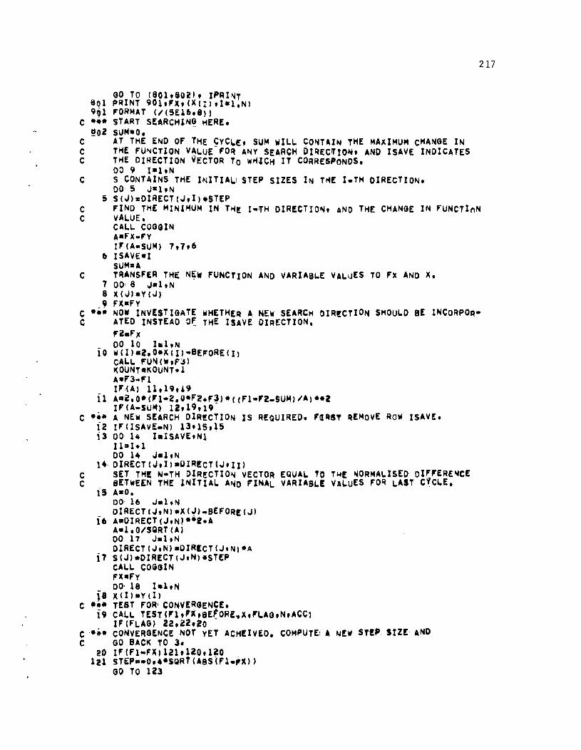
GO TO (801.8021. IPRI~T 801 PRINT 901.FX,IXI!),Ial,N) 901 FORMAT 1/15E16"'1
C *.- START SEARCHING HERE. !!!02 SUM-Of
C AT THE END OF THE CYC~[. SUM wILL CO~TAIN THE MAXIMUM CHANGE IN C THE fU~CTION YALUE-FO~ ANY SEARCH DIREC'lO~' AND ISAYE INDICATES C THE DIRECTION VECTOR TO wHJCH IT CORRESPONDS.
DO 9 I-l.N C S CONTAINS THE INITIA~I STEP SIZES IN T"! I.TH OIRECTION.
DO 5 J a l.N 5 S{J).DIRECTIJ,I).STEP
217
C FIND THE MINIMUM IN TH! I-'H DIRECTION. AND THE CHANGE IN fUNCTInN C yAL.UE.
CAL.L COGGIN AaFX .. FY III'{A-SUM) 7.7,6
6 !SAVE-I SUMaA
C TRANSFER THE N~W FUNCTION AND YARIABL.E VALUES TO FX AND X. 7 00, 8 Jal.N 8 X{J)aY{J) 9 FX-FY
C * •• NOW INYESTIGATE WHETHER A NEW SEARCH OIR!CTION SMOULD BE INCORPOA· C AT ED INSTEAD O~ THE ISAVE DIRECTION.
,-Z.FX 00 10 la1.N
10 w(I).2.0*X{I)-BEFORE{I) CALL FUN O",J) KOUNT.KOUNh 1 A_F3 .. Fl III'",) 11.19,19
11 A.i.o-11I'1-2.U.F2.F~)*((F1-'2_SUM)/AI**r IF{A-SUM) 12.19.19
C *i- A NEW S~ARCH DIR!CTION IS REQUIRED. '~RST REMOyE ROW ISAYE. 12 IF{ISAYE-Nl 13,15,15 i3 00 14 I.ISAYE.N1 .
11-1+1 DO 14 J.l.N
14 OIRECT{J,I).UIR!CT'J'II) C SET TH! H-TH DIR!CTIO~ VECTOR EQUAL TO T~E ~ORMALISED DIF'ERE~CE C B!~WEEN THE INITIAL AND FINAL YARIA8LE VALUES FOR LAST C~CLE.
15 A-O. DO' 16 J.1,N OIRECTIJ,N).X{~)-8EFOR!IJ)
16 A.OIRECT{J,N)**e.A A-l.O/SQRT(AJ DO 17 J_l.N OIRECTIJ,N).DIRICT{J'NI*A
i7 SeJ).OIRECTIJ,N)*STEP CALL COGGIN FX~Fy
00· 18 I.1.N is x{I)·Y(I)
C ... TEST FOR' CONVERGENCE. 19 CALL TESTC'1,'K.eE'ORE~X"LAG.N.ACC1
IF(FLAG) 22,Z2,20 -C*** CONYERG~NCE NOT yET ACH!IYEO. COMPUTE: A ~EW STEP StZE AND C GO BACK TO 3.
20 IF(Fl-FX)121.120,120 111 STEP •• 0 •• *SQR1CAsslFl.;X»)
GO TO 123

218
120 123
21
c··· c
STEP.0 ••• SQRTeF1·FX) IFeSTEPA.STEP) 21.j.3 STEP.STEPA -GO TO 3 CONIIERG!NCE ACHEI vEO. I F I CONVGa2' I ""C~EASe:. AL.L. VIR U8L.£~ BY lO-ACC AND GO BACK~TO 3.
22 GO TO c23.24).ICONVG 23 RETURN 2~ GO TO e25.21"NTRY 2S NTRY.2
DO 26 h1,N FlRST(PdII)
~6 XII)-XtII+ACC*10.
C *it. C
FFIRST-FX GO TO 100 CONIIERGENCE ATTAINED USING TWO 01"E~e:~T STIRTINij POINTS. CONSTR~C UNIT VECTOR i~~W!EN SOLUTIONS AND SElRCH DIRECTION FOR A MINI~U".
27 FSECNOa'x A-O. DO 28 h1.N SECNO(II.XII) $(I).'IR$TII)·SECNDCII
28 AaA+$ll).*2 . IF(AI 23,i3,29
29 AaSTEP/SQRT(A) DO 30 b1,N
30 S Cl) as C I I .A CALL. COGGIN TEST IF NEW POINT IS SU"I,IENTL.Y C~OS!i TO EITHER OF TH£ TWO SOL.UTIONS. IF So RETURN. CAL.L TEST('FIRST,F~.FIRST.Y.FLAG.N~ACC' IFeFLAG) 32.J2,31
31 CAL.L. T!ST('SECND,FY.S!CNo.Y.'L.'G.N~ACCt IFiCf"L.ACU 32.32.34
32 DO 33 I-l,N 33 )( ( 1).y C IJ
FX-Fy RETURN FINAL. SOL.UTION NOT ACCURAT! tHOUGH. ~EPLACE THE FIRST DIRECTION VECTOR By INTER.SOLUTION VECTOR CNO~~A~~SEOI AND RECYCLE
C *it. C
3~ AaA/STEP . . DO' 35 hl.N DIRECTeI.1)aiFIRSTeI'·SECHDCI»*A
35 FIRST(I)aSECNoel) GO TO 3 EtliO SUBROUTINE TEST eFI ." .RI .R,.FLAG,H,. ACC,) DIMENSION RI(~0).~F(10) FI..AG .. 2. IF(ABS(FI)·A~C) 2.2.1
1 IF(ABS((FI.FF)/FI)~ACC1 3.3.7 2 IFi(ABS(FI·prF)·~CCI 3.3.1 3 00 6 Ia·l./II
IF~ABS(RICI».ACC) 5.5.4 4 IF(ABS«RI(I).RF(I»/~i(I».ACC) 6'6,7 5 I";(AE;SC~I(I)-R~<I».ACC') 6 .. 6.7 6 CONTINUE
FL.AG ... a. 7 REITURN
END SUBROUTINE COGGIN COMMON IONEI X,Y.~,fX.FY'N.KOUNTSfLIN.NnRV'H,S'G'O!LG

219
C ••.• DIMENSION XIIO)'YIIOI.SIIO).SleCIO)'OE~GCIO"HII0'lg) TME INITIA~ VARIABLE VALUES ARE IN x. AND THE CORRESPON l~G
C .~. FUNCTION VALUE IS FX.· C·.· THE SEA~CH DI~~CTION VECTOR IS S. A~D TH! INITIAL STEP SIZE STEP. C ••• ~IN IS USEO TO COUNT THE NUMBER or 'UNCTto~ EVALUATIONS A~O N IS C ••• THE NUMB[R OF VARIABLEs. -
FA-FB·FC.FX DA-De-DC.O. STEPal.O O-STEP 1<--2 M-O
C ••• START THE SEARCH THE BOUNO, THE MINll4UIII 1 DO Z I-l.N -2 VII)-XtI)+O.5CI)
CALI.. FUNCV,F) K·I(+l LIN-LIN·l IF,IF .. FA) 5,3,'
C ••• NO CHANG! IN 'UNCTION VALUE. RET~RN wITH vICTOR CORRESPO~OING Tn C 'UNCTION VALut OF EA, BECAUSE IF THE FuNeTION VALUE IS I~OEPENDE~T C of TMIS SEARCH OIRECTION, THEN CHANGES IN THE VARIABLE VA~UES MAv C uPSET THe: MUN PRO~RAI4 CONVERGENCE T!STl~G.
3 00·. I-l.N • YII)-XII)+DA·SII)
"V-FA RUURN
C ••• THE FUNCTION IS STILL DECREASING. I~CR!&SE' THE STEP SIZE, 8Y C DOUBLE THE PR~VIOUS INCAEASE IN STEP SIZ!.
5 FC-F8 S F8-'A S FA_I" DC-De 5 OB-OA S DA_D o-Z.O*O+STEP GO TO 1
c *i. MINIMUM IS 80UNDED IN AT LEAST ONE Dl_ECTION. 6 I"CKI 7,8,9
C MINIMUM IS BOUNDED IN oNE DIRECTION ONLW. REVERSE THE SEARCH C DIRECTION AND RECV~LE.
7 Fi-F . 08-0 S D-.U S STEP •• &TlP GO TO 1
C MINIMUM IS BOUNDED IN BOTH, DIRECTIONS AFTEQ ON~Y T~OI'UNCTION C EVALUATIONS tONE EITHfR SIDE OF TME ORI8tN). PROCEED TO THE C PARABO~IC INTERPOLATION.
S Fe-FB S Fa-'A S- FA.' DC-DB I OB-DA S DA.O GO TO Zl .
C THE MINIMUM IS BOUNDED AFTIR AT LE.ST TWO "UNCTION EVAL~ATIONS IN C THE SAME DIREC~ION. E~ALU'T[ THE FUNCTION AT sTEP SIZE-IOA·DB)/z. C THIS WI~L YEIL~ 4 'QUA~LV SPACED POI~TS BOUNDING THE MI~~~U~.
9 DC-DB S oa-OA S DA_D FC-FB S FB.,A $ 'A.'
10 0-0.5*(OUOB) 00 11 l.l.N
il V(II.X(I)+O*S«II CALL FUN(y,F) . LIN-LIN+l
C ••• NOW HAV~ THAT FA~FBc,c AND THAT 'A.'~'C ASSUMING THAT THE C FUNCTION IS UNIMODAL. REMOVE EITHER POl~T A OR POINT 8 IN SUCH i C WAY THAT THE ~UNcTtON is BOUNDED AND Fl)'ec,C tTHE CORRESPONDINI C STEP SIZES ARE DA~DB>DC OR DA~DBcOC 1.
}2 IF« 10C.D) *CO·08), 15'13.18 C ••• · LOCATION 0, MINIMUM IS LIMIT!O BY ROUNDING ERRORS. RETURN WIT~ B.

220
13 DO, 14 hl.N 14 YIII.XCII.OS-SIII
n'.FB RETURN
C ••• T~E POINT 0 IS IN THE RANGE OA TO OS. 15 IF~F.FB' 16.13.17 16 Fe-Fe S Fe.'
DC-DB S oe-o GO TO 21
17 FA.F OA*O GO TO 21
C •• 0 T~E POINT 0 IS I~ T~E RANGE DB TO DC 18 IFCF.FB) 19.13.20 19 FA-Fe S Fa.,
Ohoe S 08.0 GO TO 21
20 Fe-F oe-o
C -.- NO. PERFORM THE PARABOLIC INT!RPO~ATIO~. 21 A-FA.(08_0C,.~B.(0~-OA).FC.(OA.08)
IF:(A, 22.30,22 22 D-O.S.C(Oa.D8·~C.OC)·'A.(DC-OC-OA-DA).FB.IOA.OA·UB.OBI .'e)/A
C CHECK THAT THE POINT Is GOOD. IF 50. [¥A~~ATE THE FUNCTIO~. IFIIOA.O).IO-D~), 13.13.23
~3 DO 24 Z.l.N l4 YCI)-XCI).O-SII,
CAL.L FUN I Y,'l LlN-L.I~·1
C ••• CHECK FOR CONVERGENCE. IF NOT ACHEIVEO. R!CYCLE. IFHBSIFa,-o.ooOOl) 25.25,26
25 A-1.0 S GO TO 27 1!6 Aal.0/F8 ~1 IFI(ABSI(FB.F)·~, ... 0001) 21"28,12
C ••• CONVERGENCE AeHEIVEO. RETURN wITH TM! SNALL.ER OF F A~O F8. 28 IF,(F·FB) 29.13~13 ' 29 FY-F ~
R[!TURN C .i. THE PARASOLIC JNTERPO~ATION WAS PAEVENTEO SY THE DIVISoR BEING C ZERO. IF THIS IS THE FIRST TIME THAT IT HAS HAPPENED. TRY AN C INTERMEDIATE STEp SIZE ANO RECYCLE} OTHERWISE 9I~E UP AS IT L.OOKS C LIKE A LOST CAUSE.'
]0 IF(M) 31,31,13 31 "'-"'.1
GO TO 10 END BI..OCK DATA COM"'ON 10NEI X.y.S.FX.FY.N.KOUNTS.~IN.NDRV.H.SI8.0ELG OIMENSI ON X (10 j • Y C1 0) ,5 I 10) • SIli (10) 'DELS 11 0) • H 110.10) DATA X(1)/40.0/,N/ll [NO ' SUBROUTINE FUN(X,FX, DIMENSION XC10)
C 'UNCTIO~ 1 paO.02S16 Ta~ 11,
C INSER~ SUBROUTINE To COMPUTE C 8·a600./C4 •• 1·P·T··I·ll0.5.1P·T) •• 1.1.561~T) C_110.2_21.11.!lopr-S*,.l.33iT.1.66'*8,/15.0 S FX_C PR,INT 1.P,T ,B,C
1 FORMATC5X'.P.·'Fl0.5'5x,.INITIA~ T •• "40.2.·B-.'El0.3,iC-.~EIO.l/) RETURN

C.2
Optimization Method of NeIder and Mead (SIMPLEX)
Instructions to Introduce Data into the Work
The Data Cards are as follows:
7 1. 8
9
221
2. Punch NX, the number of variables in the objective function in format
(IS) in col. 1-5 right justified, and STEP, the step size in format
(FlO.S) in columns 6-15. In the absence of other information select
STEP = min (0.2 ~ di
' dl
,d2
, ... ,dn
) n i=l
where n = no. independent variables and d. is the possible region for ~
search for the variable x .. ~
3. Punch the initial guess for each variable in format (FlO.S).
Cards 2,3 can be repeated changing the step size and intial variables
as desired, but after last card of type 3 must come:
4. Blank card
6 S. 7
8 9
The card (SUM(IN) = f(x)), the third last card in the deck, must be changed
for each different function. Allowance has been made for a 50 dimension
problem, i.e., X(l) to X(SO).

222
PROGRAM $IMP~[XIINPUT.OUTPUT) C ••••• OP~IMIZATION BY THE NELDER-MEAD M!~~OO ••••• C NX IS THE NUMB~R O~ INOEPENDENT VAR1A8~EI. C STEP IS THE INITIA~ ST!P SIZE. C XII) IS THE ARRAY OF I~ITIAL GUESSES. C DATA CARDS ARE AS FOL~oWS. C CARD NO. PARAMETERS C 1 NX C 1 STEP C 2 XII) C CARD 3 IS BLANK.
FO"MAT t5 "10,15 "10.5
CO~UMNS 1 TI'iRU !5 6 THRU 15 1 THRU 10
e TO OPTIMIZE THE OBJECTIVE FUNCTION FOR A~OTHER SET OF PARAMETERS C REPEAT CARDS 1 AND 2 ONLY. C FOR PROPER PRINTOUT OF DESIRED XII) ARR6V. FORMAT STATEMENTS 103 C AND 101 MUST SE REVIS~O ACCORDING~¥.
DIMENSION Xl(SO,50I, X(50), SUMISO) COMMON/ll x,Xl,NX,STEP.K1,5UM,IN
1 FORMATIII,FI0.S) 100 READ1, NX,STt~
H';(NX) 998,999.998 998 READ 2, IX(II,I.l,NX)
2 FORMATII0FI0.51 AI..'A-l.0 eEiTA-o.5 GAMb2.0 oIFER • O. X,...~ • NX IN - 1 CALL lUNA PRINT 102,SU'Hll,(XCI"I-1,NXI
PRINT lO02,STEP CALL SECQNO(T1ME) PRINT 1 O!St TIME
lOS FORMATI/!OX,liHTIME IS Now,F10.3,BH SECONDS/) PR~NT 103 .-
103 FORMAT(~X,14HFUNCTION ijALUE'15X,3HX1 •• 20X,3HX2.'iO~'3HX3.,lOX,3Hx4 1-,16X,12HFUNC~ CHANGE)
102 FORMATclH1,IZX,23H~UNCTION STARTING VALU!,F10.S,I,.THE X ARRAV I~. 1.I,5X,10CEll.·,2X»
1002 'ORMATI12X,.ST~P ••• F6.2) 1(1 • NX • 1 1(2 • NX • 2 1(3 - NX • 3 I(~ • NX • 4 CALL START
~5 DO 3 I • 1, K1 00 It J a· 1. NX
4 XIJ) • XIII ,J) IN - I CALL SUNR
3 CONTINUE c SELECT LARG[ST VALUE OF SUMCI) IN SIMPLEK
21i SUMH • SUM (1' INDEx • 1 DO 7 I ., 2. Kl I'iISUMll) ,LE.SUMH) 90 TO 7 SUMH • SUM I %) INDEX II! I
7 CONTINUe: c SELECT MINIMUM VALUE 0' SUM(I) IN SIMP~EK
SUML - SUM (1)

KC)UNT • 1 00 8 I • 2. 1\ 1 IFiCSUML.,L.E,SUMCI" GO TO 8 SUML. ill SUM e I I t<OUNT • I
8 CONTINUe: C FINO CENTROID OF POINTS ~ITH I DIFFERENT THAN INDEX
DO 9 J •. 1. NX SUM2 • 0, DO' 10 I • 1. I< 1
10 SUM2 • SUM2 • Xl(I.JI xl1K2.JI al./XNX*ISUMZ • XlIINOEX.Jll
C FJNO REFL.EC,ION OF HI~H POINT THROUGH CENTROIO XlIK3'JI • 11, • AL.F"ixlCK2.J) • AL.'A*Xl~INOEX'Jl
9 XIJl • XlCI<3,JI IN' • 1<3 . CAL.L. SUM,. IFIISUM (1<3) .L. T ,SUML.J GO TO 11
C SEL.ECT SECOND L.ARGEST VALUE IN 5IMPL.[K IFCINOEX.EQ,11 GO TO ,. SUMS • SUM (l I GO TO J9
,8 SUMS. SUMCZI 39 D~ 12 I • 1. 1<1
I'~CINDEX .. ll.[Q,DI 10 TO 12 I,ijSUMCIl,L.!.SUMSI GO TO 12 SUMS. SUM U I
i2 CONTINUE:-I'I(SUMI1<31,GT.SUMSI GO TO 13 GO, TO 14
C ;ORM EXPANSION 0' NEW MINIMUM IF AEFL.ECTION HAS PROUUCEO ONE MINIMUM 11 DO' 15 J • 1. NX
xl (K4.JI • C 1 .. GAMAI.Xl IKZ.JI • GAMA*K1 CI(3'JI i5 X(JI • Xlll<4.JI
IN • K4 CAL.L. SUMR l'iISUM(1(41,L.T e SUML.) GO TO 16 GO' TO U
i3 IFIISUM(I<31,GT.SUMHI GO TO 17 DO' 18 J • 1. NX
18 XlIINOEX.Jl • XICKJ.JI 17 00· 19 J • 1. NX -
xl(K4.Jl • 8ETA*XlIIND£X.JI • II, ... aETA~iKIIK2.JI 19 x IJI • Xl Ct(4.JI
IN • 1<4 . CALoL. SUM" IFI(SUMH,eT ,SUM IK411 GO To 16
C ~EOUCE SIMPL.EX eY HALoF I' REFL.!CTION HAPPEN! TO PROOUCE A L.ARGER VAL CLUE THAN THE MAXIMUM •
00' 20 J • 1. NX DO' 20 I • 1. K.1
!O xl1I.JI • 0.5.IX11~.Jl • XleI<OUNT,J,1 DO 29 I • 1. 1<1 DO' 30 J • 1. NX
30 xeJI • Xl(1 • ..I) IN II I CAL.L. SUMR
29 CONTINUE GO· TO 26
i6 DO 21 J • 1. NX xlIINOEX.Jl • X1CK4.JI
21 xeJI • XleINOEX.JI·
223
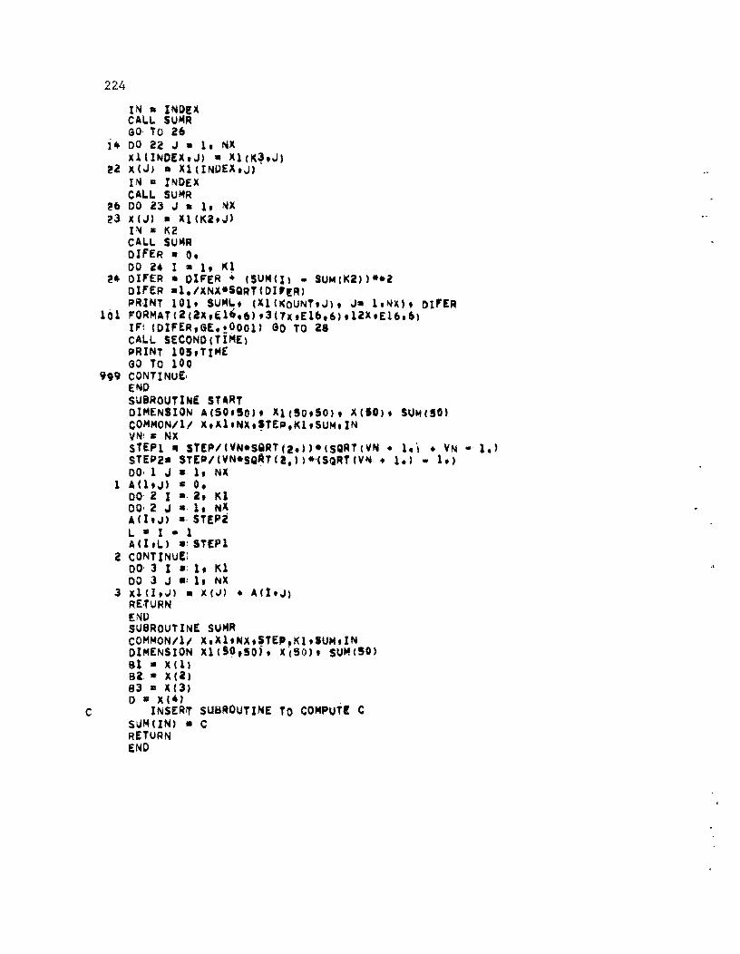
224
IN • INDe:X CALL SUMR GO' TO 26
}4 DO 22 J - 1, NX xllINDEX,JI - X1CK3.J)
!2 X (J) • )(1 CINIlEX,J) IN • INDEX CALL SUI4R
!~ DO 23 J • 1. NX 23 X (J) • Xl (K2.J)
It\4 • 1<2 CALL SUI4R DIFER • O. DO 24 I - 1. 1<1
!4 DIFER • DIFER • (SUNCI) • SUMCK2»**Z DIFER .1,/XNX*SQRTCDlr!RI PRINT 101. SU~L. (llCI(OUNT.J). J- 1.NXI. DI'ER
101 FORMATC2C2x.El'.6).3(7X.E16.6).12X.E16.6) IF: COIFER.BE,!.OOOl) BO TO 28 CALL SECONDCTI"E) pRINT lOS.TIME GO To 100
999 CONTINuE, END SUBROUTINE ST_RT DIMENSION ACSO.50). Xl(50.50). X(IO). SUM(!Ol COMMON/ll x,Al'NX.,TEP.Kl.SUM.IN VN' • NX STEPl • STEP/CYN*SQRTra,»*CSQRTCYN • 1,~ • YN • 1.) sTEP2- STEP/(YN~SQATC2.')*1SQRT(YN • 1,) • 1.) DO- 1 J • 1. NX
1 An.J) • 0, 00 2 I ., 2. 1<.1 00' 2 J • 1. N~ A (I.J) a' STEPi L • I • 1 A cI ,L) .' STEP 1
2 CONTINUEI 00· 3 I .' 1. 1<.1 00 3 J .: 1. NX
3 X1CI.J) .. xeJ) • A(ItJ) RETURN ENIl SUBROUTINE SUMR COMMON/ll X,Xl.NX.5TE',Kl,SUM.IN DIMENSION X1CSO.50;. X(50). SUMeSO) 81 - X Cl) B2 • X(2) 83 • 1((3) D • XC.)
C INSER~ SUBROUTINE TO COMPUTE C SUM tIN) • C RETURN END

C.3
SUbROUTINE TO CALCULATE. THE ObJECTIVE FUNCTION FOR 2-SPAN DOUBLE BOX GIRDER BRIOGE
NOTATION
CONSTANTS B TOTAL WIDTH B6 WIDTH OF CAST-IN-PLACr STRIP T4 WEB THICKNESS
VARIA8LES FROM MAIN PROGRAM 81 WIDTH OF CANTILEVER OVERHANG 82 FIRST INTERIOR SPAN OF DECK 83 WIDTH OF BOTTOM SLA8 D DEPTH OF SECTION
QUANTITIES CALCULATED A AVERAGE SECTION AREA AS CABLE AREA C OBJECTIVE FUNCTION
B = ::>0. B6 = 2. T4 = 1.0833 GO TO 5
2 PRINT 2iJOC, B1, B2, B3, D 2000 FORMAT (*Bl 82 83 D =*, 4E12.2)
CALi... eXIT 5 CONTINUt.
TIl = .7 10 F1 = .025*(1.+T11)*81**2 + 26.*(B1-2.)/IB1+2.6875l
IF (d1.LE.8.) GO TO 20 F1 = F1 + 26.*181-8.)/(81-3.3125)
2U T1 = .167 + .1268*SQRTIF1) E = ABSIT1-T11) IF (E.-.v01) 40,40,30
30 TIl = T 1 GO TO 10
40 IF (T1.LT •• 5) T1=.5 W = 8-2.*Bl-4.*T4 B5 = W-2.*B2 T5 = O. IF Ib5.LE.U2) GO TO 70 T51 = .5
50 F5 = .OI25*T51*~5**2 + .52*(85+2.) T5 = .167 + .1268*SQRTCF5) E :; ABS ITS-T51 ) IF ([-.vOl) 70,70,60
60 T51 = T5 GO TO 50
70 CONTI NUE
225

226
T21 = .5 8U F2 = .0125*T21*B2**2 + .52*(R2+2.)
5T2 = T21**3/B2 5 = SQRT( (D-T21-.5)**2+( (H2-H3)/2.+T4)**2) 5T4 = .75*T4**3/S F2 = (5T4*F2+ST2*Fl)/(ST2+ST4) T2 = .167 + .1268*SQRT(F2) E = ABS!T2-T21) IF (E-.OOll 100,100,90
90 T21 = T2 GO TO 80
100 IF !T2.LT •• 5) T2=.5 IF (T2.LT.T5) T2=T5 AA1 = 81*(Tl+.5)/2. II = (T1**2+.5*Tl+.25)/(Tl+.5)/3. AA2 = «8-B6)/2.-B1>*T2 l2 = T2/2. AAT = AA1 + AA2 AlT = AA1*ll + AA2*l2 AA3 = B3*.5 l3 = D-.25 AA4 = 2.*S*T4 l4 = (U-.5+T2}/2. All = AAT + AA3 + AA4 Al = AlT + AA3*l3 + AA4*l4 DCl = Al/All H = u-.~*DCl-l.00~ A5 = All/(19.2*H) Al = 2.*All + 86*T2 BMD = 820.*(Al+.113*(B-Z.» BMS::: tl50.*All*(1.-(DCl-.67)/H) BMU = 8MD + 25260. - R~S
T31 = 1. J = 0
110 DM = D-.5*T31-.67 T3 = 8MU/(1322.*DM*B3) E = A85(T3-T31) J = J+l IF (J. G T .20) GO TO 2 IF (E-.GOl) 130,130,120
120 T31 = T3 GO TO 110
130 IF !T3.LT •• 5) T3=.5 ASU = BMU/(31100.*DM) IF (A5U.GT.AS) AS=ASU Q = 1./12.
140 Q = Q+l./36. DM = D-.92-1.7*Q*(D-l.34) BMU = 661.*DM*83 BivJX = Bj'ID*11.-5.*U+4.*Q**2) + 12630.*(1.-Q) - R~':S*(I.-Q)
IF (BMX.GT.BMUl GO TO 140 AA3 = B3*T3 S = ~QRT( (D-T2-T3)**2+( (B2-83)/2.+T4)**2) AA4 = 2.*S*T4 AT = 2.*AAT + 86*T2 A2 = AT + 2.*(AA3+AA4)

227 A = Al + CAZ-All*Q/Z. C = 5.345*A + 343.*AS + .031*!R+3.*D+IO.I*D
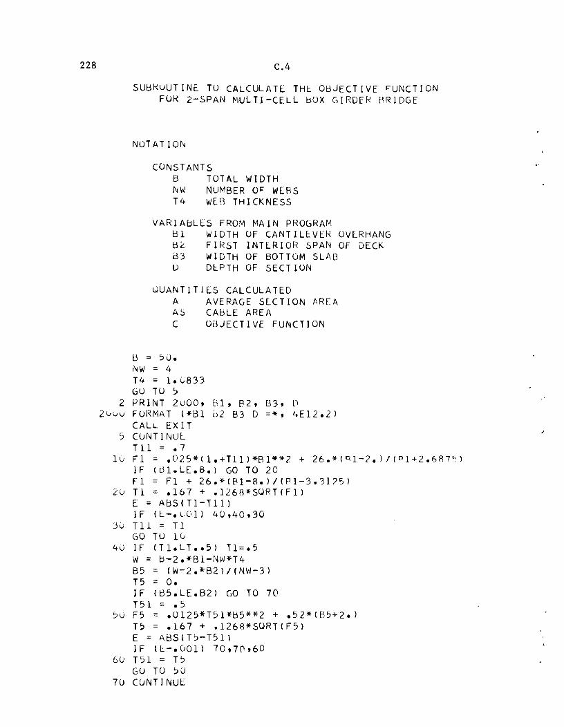
228 C.4
SUBkUUTINE TO CALCULATE THE OBJECTIVE FUNCTION FUk 2-SPAN MULTI-CELL BOX GIRDER RRIDGE
NOTATION
CONSTANTS B TOTAL WIDTH NW NUMBER OF WERS T4 WEG THICKNESS
VARIABLES FROM MAIN PROGRAM B1 WIDTH OF CANTIL~VER OVlRHANG 6~ FIRST INTERIOR SPAN OF DECK 63 WIDTH OF BOTTOM SLAB U DEPTH OF SECTION
uUANTIT1ES CALCULATED A AVERAGE SECTION AREA AS CABLE AREA C OdJECTIVE FUNCTION
B = ~0. NW = 4 T4 = 1.0833 GO TO :,
2 PRINT 2000, B1, 82, B3, D 2uuu FORMAT (*81 u2 83 D =*, 4EI2.2)
CALL EXIT 5 CUNTINUl
T11 = .7 10 Fl = .025*(1.+Tl1)*B1**2 + 26.*(Rl-?I/(nl+2.6R7~1
I F (tl1. L E • 8 .) GO TO 2 ° Fl = F1 + 26.*(Bl-S.)/(Pl-3.31?5)
20 T1 = .167 + .1268*SQRT(Fl) E ::: AbS<TI-Tll) IF (E-.LJC!ll 40,40,30
30 T11 = Tl GO TO 10
40 IF tT1.LT •• 5) T1=.5 W = b-2.*B1-NW*T4 B5 = (W-2.*B2)/(NW-3) T5 = O. IF (B5.LE.B2) GO TO 70 T51 = .5
5U F5 = .0125*T51*65**2 + .52*(B5+2.) T5 = .167 + .1268*SQRT(F5) E = AbSCT5-T51) IF (E-.OOl) 70,70,60
60 T51 = T? GO TO :'0
70 CUNTINUE

T21 = .5 80 F2 = .0125*T21*82**2 + .52*(P2+2.)
5T2 = T21**3/82 5 = SOkT( IO-T21-.5)**2+( (8-63)/2.-Bl)**2) 5T4 = .75*T4**3/S F2 = (ST4*F2+ST2*Fl)/(ST2+ST4) TL = .167 + .1268*SORT(F2) E=ABSIT2-T21) IF (E.-.uOll 100,100,90
'Ju T21 = Tt: GO TO 80
luO IF 1T2.LT •• 5) T2=.5 IF 1T2.LT.TS) T2=T5 AA1 = 81*(T1+.5) Zl = (T1**2+.5*Tl+.25)/(Tl+.5)/3. AA2 = (B-2.*61)*T2 Z2 = T2/2. AT = AAI + AA2 AZT = AAl*Zl + AA2*Z2 AA3 = 83*.5 l3 = D-.25 AA4 = ((NW-2)*(D-T2-.5l+2.*Sl*T4 Z4 = (D-.5+T2)/2. Al = AT + AA3 + AA4 Al = AlT + AA3*l3 + AA4*l4 OCI = Al/Al H = U-.5*DCl-l.005 AS = Al/(38.4*H) BMD = 820.*(Al+.113*(B-2.)) Sf-1S = 425.*Al*(1.-(DCl-.67)/H) bil,lU = 8i'lD + 25260. - 8MS T31 = 1. J = 0
110 UM = 0-.5*T31-.67 T3 = BMU/(661.*D~*B3) E = AbS(T3-T31) J = J+l IF (J.GT.20) GO TO 2 IF ([-.001) 130,130,120
120 T31 = T3 GO TO 110
l30 IF (T3.LT .. 51 T3=.5 A5U = BMU/(31100.*DM) IF (A5U.GT.AS) AS=ASU Q = 1./12.
140 CJ = (.)+1./36. DM = D-.92-1.7*Q*(D-l.34) BMU = 330.5*DM*B3
229
BMX = BMD*(1.-5.*~+4.*Q**2) + 12630.*(1.-Q) - BMS*(I.-Q) IF (BMX.GT.BMU) GO TO 14C AA3 = B3*T3 S = SORT( IO-T2-T3)**2+( ([1-B3)12.-Bl )**2) AA4 = ((NW-2)*(D-T2-T3)+2.*S)*T4 A2 = AT + AA3 +AA4 A = Al + (A2-Al)*Q/2. C = 5.345*A + 343.*AS + .C31*(6+3.*0+10.)*D

230 c.s
SUBR0UTINE T0 CALCULATE THt OBJfCTIVf FUNCTION FOR 3-SPAN DOUBLE BOX GIRnFR RRIDGE
1\10TAT101,<
CUNSTANTS B TOTAL WIDTH B6 WIDTH OF CAST-IN-PLACF STRIP T4 WEB THICKNESS
VARIABLES FROM MAIN PROGRA~
Bl WID1H OF CANT1LEVfR OVERHANG B2 FIRST INTERIOR SPAN OF DECK 83 WIDTH OF HOTTOM SLAR U DEPTH OF SECTION
~UANTIT1ES CALCULATED A AVERAGE SECTION AREA AS AVERAGE CARLr AREA C adJECTIVE FUNCTION
B = 56. B6 = 2. T4 = 1. GO TO ?
2 PRINT 2uOO, Ul, B2, 03, D 20v0 FORMAT (*61 H2 63 D =*, 4[12.21
CALL EX IT 5 CONTINUl
TIl = .7 10 Fl = .025*(1.+Tl1)*Bl**2 + 26.*(H]-2.1/(Rl+2.68751
I F ([< 1 • L E • 8 • 1 GO TO 2 (1
F1 = Fl + 26.*IBl-8.)/(nl-3.31251 2J Tl = .167 + .126R*SQRTIFll
E = ABSITI-Tlll IF It-.GOl) 40,40,30
30 T 11 = T 1 GO TO 10
4u IF (Tl.LT •• 5) Tl=.5 W = 6-2.*81-4.*T4 B5 = W-2.*B2 T5 = c. IF (~5.LE.B21 GO TO 70 T51 = .5
5U F5 = .0125*T51*65**2 + .52*(B5+2.) T5 = .167 + .1268*SQRT(F5) E = ABS(T5-T51) IF (E-.GOl) 70,70,6U
6U T51 = T5 GO TU ?U
70 CONTI NUE
.'

..
T21 = .5 eo F2 = .0125*T21*B2**2 + .52*(B2+2.)
ST2 = T21**3/B2 S = SQRT«D-T21-.5)**2+( (R2-B3)/2.+T41**2) ST4 = .75*T4**3/S F2 = (ST4*F2+ST2*F11/(ST2+ST4) T2 = .167 + .126A*SQRT(F2) E = A BS ( T 2 - T 2 1 ) IF (E-.OOll 100tlOO,90
90 T21 = T2 GO TO 50
1uO IF (T2.LT •• 5) T2=.5 IF !T2.LT.T5) T2=T5 AA1 = B1*(T1+.5)/2. II = (T1**2+.5*T1+.25)/(T1+.5)/3. AA2 = «B-B6)/2.-B1)*T2 l2 = T212. AAT = AA1 + AA2 AlT = AA1*ll + AA2*l2 AA3 = B3*.5 l3 = D-.25 AA4 = 2.*5*T4 l4 = (D-.5+T2)/2. All = AAT + AA3 + AA4 Al = AlT + AA3*l3 + AA4*l4 DC1 = Al/A11 BMU = 1C12.5*A11 + 5344. T31 = 1. J = 0
110 DM = D-.5*T31-.46 T3 = BMU/(661.*DM*B3) E = ABS(T3-T31) J = J+1 IF (J.GT.2C) GO TO 2 IF (E-.OOll 130tl30tl20
120 T31 = T3 GCJ TU 110
130 IF (T3.LT •• 5) T3=.5 ASU = BMU/(31100.*DM) DM = D-.71 BMU = 330.5*DM*B3 Q = .05
14(J Q = Q+.U5 BMX = l012.5*A11*(1.-Q)**2 + 5625.*(.95-Q) IF (~MX.GT.BMU) GO TO 140 AA3 = B3*T3 l3 = D-T3/2 S = ~QRT(~D-T2-T3)**2+( (E2-B3)/2.+T4)**2) ftA4 = 2.*5*T4 l4 = (D-T3+T2'/2. A21 = AAT + AA3 + AA4 Al = AlT + AA3*Z3 + AA4*l4 DC2 = Al/A21 Al = 2.*All + B6*T2 A2 = 2.*A21 + A6*T2 A = Al + (A2-AI,*Q/2.
231

232
ASI = .0386*All/(DC2-.461 IF (ASU.GT.ASII ASl=ASU AST = .43*ASI DEC = 1)-.5-DCl AS21 = .15 J = 0
150 BMS = 8980.*AS21*DEC BMU = 445.5*(Al+.113*(B-2.11 + 16850. - 396.*A11 + RMS DM = D-.5-26.*AS21/B AS2 = BMU/(34340.*DMI E = ABS«AS2-AS211/AS211 J = J+l IF (J.GT.2U) GO TO 2 IF (E-.002) 170,170d60
160 AS21 = AS2 GO TO 150
170 ASB = .475*AS2 AS = AST + ASS C = ?345*A + 343.*AS
,.