The Demand for Primary Schooling in Madagascar: Price, Quality, and the Choice Between Public and Private Providers

Peter Glick* and David E. Sahn

Cornell University

January, 2005

Abstract We estimate a discrete choice model of primary schooling and simulate policy alternatives for

rural Madagascar. Among school quality factors, the results highlight the negative impacts on

schooling demand of poor facility quality and the use of multigrade teaching (several grades

being taught simultaneously by one teacher) in public schools. Simulations indicate the

feasibility of reducing multigrade in public schools by adding teachers and classrooms, a policy

that would lead to modest improvements in overall enrollments and would disproportionately

benefit poor children. Given much higher price elasticities for poorer households, raising school

fees to cover some of the additional costs would strongly counteract these favorable

distributional outcomes. An alternative policy of consolidation of primary schools combined

with multigrade reduction or other quality improvements is likely to be ineffective because of the

strongly negative impact of distance to school.

JEL: I2, O15

Keywords: Education, school quality, human capital, school choice, Madagascar *Corresponding author: Peter J. Glick, Cornell University, 3M12 MVR Hall, Ithaca, NY, 14853, Telephone 607 254-8782, E-mail: pjg4@cornell.edu

2

I. INTRODUCTION

The provision of free or largely subsidized primary education is among the most

important and widely accepted functions of governments in developing countries. In Africa,

however, after impressive successes following independence, governments have faced increasing

challenges to fulfilling this function. In part as a consequence of economic stagnation and

decline beginning in the early 1980s, public education systems in African countries have

suffered from severe revenue shortfalls during a time when the school-age population has grown

rapidly. Inevitably, quality has deteriorated in public schools, which together with the effects on

education demand of falling household incomes has left many countries far from achieving basic

goals of universal primary enrollment and literacy. At the same time, growing dissatisfaction

with the public education system has led to a rise in the demand for private schooling.

Faced with these trends, governments must attempt to meet several important but

potentially conflicting objectives: to improve school quality, to restore or increase enrollment

levels, and to insure that public spending on education is progressive (or ‘pro-poor’). The

potential conflicts are well illustrated by the controversy generated by proposals to impose or

increase public school fees. This may make it easier for governments to invest in much needed

quality improvements or new school construction, but serious equity concerns have been raised:

will the higher costs impinge the most on enrollments of the poor?

A complicating factor for policy (and analysis) is the presence of a private sector in

education. Substitution between public and private school alternatives will influence the

outcomes of education policies even when these policies are implemented only in public schools.

For example, the negative enrollment impacts of public school fee increases may be offset by

increased private enrollments, with the extent depending on the availability of private

alternatives and the magnitude of the cross-price elasticity. At the same time, the goal of the

3

price increase, to raise revenue for the public schools, will be confounded by the exodus of fee-

paying students from the public sector.

Although a number of studies for developing countries have examined the role of price

and quality in schooling decisions, very few have looked at how these factors influence the

choice between public and private school alternatives.1 Further, few have attempted to compare

alternative education policies with respect both to schooling outcomes and public sector costs.

We address each of these issues in the present study, using a detailed household dataset from

Madagascar that is complemented by data on the characteristics of local schools. We estimate

the effects of changes in price and school characteristics on the primary schooling decisions of

rural households, incorporating the private sector as an alternative to public schools. After

clarifying analytically the relationship between price elasticity estimates obtained from demand

models and changes in the benefit (school enrollment) shares of different quintiles of the income

distribution, we use the estimates to simulate the impacts of pricing and other policies on public

and private primary enrollments and their distribution across household expenditure quintiles.

In particular, we consider these outcomes and the associated costs to the government of a

policy of providing additional teachers and classrooms in public schools to reduce multigrade

teaching, a widespread practice in Madagascar and other developing countries whereby a single

teacher must teach two or more classes at once. We then investigate the distributional and

budgetary implications of combining these improvements with cost recovery, i.e., increases in

school fees. We compare these outcomes and costs to those for an alternative strategy to

improve school quality that often arises in policy discussions: school consolidation, under which

some small rural schools are closed and the cost savings are used to improve the quality of

nearby schools.

1 Alderman et. al. (2001) and Younger (1999) are among the few exceptions.

4

The paper is organized as follows. The next section describes the empirical strategy.

Section III describes the institutional background and the data, and Section IV presents the

results of the estimations and policy simulations. Section V concludes with a discussion of the

policy implications of the results.

II. MODEL AND EMPIRICAL SPECIFICATION

Model of School Choice

As usual, parents are assumed to derive utility from the human capital of their children,

which is a function of their schooling, and from consumption of other goods and services. Faced

with the options of enrollment in public school, enrollment in private school, and non-

enrollment, parents choose the alternative that brings the highest utility. Define Yi as household

income and Pij as the costs to the household of choosing schooling option j (inclusive of fees and

other direct expenses as well as the value of the forgone household or enterprise production of

the child if j is chosen). Consumption net of schooling is therefore Yi - Pij if j is chosen. Also let

Sij be the increment to the child’s human capital associated with a year’s enrollment in this

school alternative. Perhaps the most frequently used functional form to represent utility is that

proposed by Gertler et. al. (1987) (see Glewwe and Gertler 1990 for a specific application to

school choice). In this specification net consumption is entered as a quadratic, i.e., for option j,

Vij = a0Sij + a1(Yi – Pj) + a2(Yi – Pj )2. The model yields an interaction of income and price,

thereby permitting the effects of price, and price elasticities, to vary with income. We employ a

variant of this approach, interacting net consumption with dummy variables indicating the per

capita expenditure quintile of the household:

Vij = a0Sij + a1(Yi – Pij )E1 + … a5(Yi – Pij )E5 + eij (1)

5

where eij is a random disturbance term. The dummy variable Ek (k =1,..,5) equals 1 if the

expenditure per capita of the individual’s household falls in quintile k and zero otherwise.

Through the coefficients on the interactions the model permits separate price responses for each

expenditure quintile. This specification permits greater non-linearity in the effects of income on

price responses than the simpler quadratic form, as well as conforming well to our simulation

exercises in which we consider the effects of policies by expenditure quintile.

The increase in human capital Sij is expected to vary across school options (one of which

is no school at all), primarily because the quality of the alternatives may differ. Since this

change is not directly observed, a0Sj is replaced by a reduced form equation for the utility from

human capital:

a0Sij = γQj + δjXi + nij (2)

where Qj is a vector of school quality variables and Xi is a vector of observed household and

individual characteristics. Many of these factors (e.g., parental education) affect utility both

through the production of human capital and through direct effects on preferences for schooling

or human capital. Substituting into (1) (and making the notation for the quintile-consumption

interactions more compact) yields

Vij = γQj + δjXi + Σka1k(Yi - Pj)Ek + εij (3)

6

where εij = eij + nij. The household chooses the schooling option j that yields the highest

utility, that is, for which Vij>Vik, all j≠k. 2

The specification developed so far is fairly standard, including with respect to the

imposition of several key restrictions on the parameters. The formulation of utility as a function

of household consumption net of schooling (Yi – Pj) imposes the restriction that the coefficient

on income is the same (times -1) as that on price. In the equation above this ‘net consumption

restriction’ is imposed for each quintile, reflected in the ak terms in (3). Note as well that these

coefficients are constrained to be the same across alternatives, i.e., there is no indexing of ak on j.

However, in our estimations our starting point is a more general specification that relaxes these

restrictions,

Vij = γQj + δjXi + Σkα1jkYiEk + Σkα2jkPjEk + εij (4)

The coefficients on Yi terms (α1jk) differ from the price coefficients (α2jk) for each quintile and

both they and the price coefficients are indexed on j. In their influential study Gertler et. al.

(1987) criticized earlier approaches that did not impose the cross equation restriction as being

inconsistent with the basic postulates of utility maximization.3 As the more recent work of Dow

(1999) brings out, however, alternative-specific effects of price (and other provider

2 As is well known, since this decision rule involves only differences in conditional utilities rather than levels,

variables in Xi that do not differ across options would not affect choice unless their effects were allowed to vary

across the options. Hence the δj are indexed on the alternative.

3 If the a1 were allowed to vary across alternatives, it would be possible for two alternatives with the same utility

from schooling γQj + δjXi and the same level of other consumption (Yi – Pj) to yield different levels of utility.

7

characteristics) would result from relaxing the assumption of separability in the utility function

between schooling and other consumption. This assumption, which is clearly imposed by the

model of eq. 3, should instead be tested. With regard to the within equation restriction relating

the income and price parameters, one situation where this restriction would not apply was

originally suggested by McFadden (1981) and arises from the presence of unmeasured tastes that

affect utility from an alternative and are also systematically related to household income. In the

appendix we present a formal derivation and show that this leads to a more general model that

nests equation (3). As described in the appendix, a likelihood ratio test rejects the restrictions

imposed by the latter. Therefore the general specification (4) is preferred.

Given the functional form for conditional utilities and the decision rule, we can derive the

demand functions, that is, the probabilities of choosing each school option. As in many previous

provider choice studies we estimate the probabilities as nested multinomial logits, a

generalization of the multinomial logit model that allows error terms to be correlated across

alternatives within a subgroup of choices. The nesting structure we adopt assumes that the error

terms of the schooling choices, which in the present case consist of public school and private

school, are correlated. An additional, less typical, aspect of our estimations is that the

probability expressions are adjusted to accommodate the fact all individuals do not have the

same number of schooling options from which to choose; specifically, a majority lack a private

school alternative. Observations with both options available contribute to the identification of

the parameters of the public and private school conditional utility functions while observations

with just public school are used to identify the public school parameters only.

Policy Simulations

We use the estimates of the school choice model to simulate the effects on primary

school enrollments of the alternative education policies described in the introduction. Since a

major objective of these simulations is to assess the distributional aspects of these policies, it is

8

important to carefully define what we mean when we say that a particular policy is beneficial or

harmful to the poor relative to the non-poor. For our analysis we distinguish two ways of

measuring these distributional effects. We illustrate the concepts using the example of a change

in school fees.

Many econometric demand studies (e.g., Gertler et. al., 1987) base their discussions of

the distributional implications of changes in fees on comparisons of price elasticities of the

“poor” and the “rich”, i.e., lower and upper quantiles of the welfare or income distribution. Here

we make explicit the connection between elasticities and changes in the distribution of benefits,

which we will define in terms of expenditure quintile shares of aggregate enrollments. Many

studies find that price elasticities are higher for low-income households, which means that the

poor’s reduction in demand from a given percentage increase in price will be greater in

proportional terms than that of the rich. Proportionately larger reductions in demand

(enrollment) in turn imply a fall in the share of the poor in total enrollments—in other words, the

incidence of primary schooling becomes less progressive in the usual fiscal incidence sense.

Formally, define Ej as the enrollments of the jth income quintile and E as total enrollment (so j’s

benefit share is Ej/E), ej as the price elasticity of the jth quintile and e as the overall or average

price elasticity, and P as the price level. It is straightforward to show that the change in the

benefit share for quintile j resulting from a change in the price is:

The elasticity of the share with respect to price is simply ej – e. Hence j’s new benefit share after

the price increase will be less than its initial share if ej exceeds in absolute value the average

elasticity. Therefore the comparison across income quintiles of the elasticities derived from

( ))ee(

EE

P1

PEE

jjj −⎟⎟⎠

⎞⎜⎜⎝

⎛=

∂

∂= sharebenefitinchange

9

behavioral models permits (inferential) comparisons of the distribution of benefits before and

after a price change or other policy.

The foregoing involves the comparison of average benefit shares before and after the

policy is implemented—it shows how the targeting of benefits to the poor changes as a result of

a policy. However, we also are likely to be interested in the marginal shares, that is, the quintile

shares in the aggregate increase or decrease in school enrollments resulting from the policy. Do

lower income quintiles incur a disproportionate share of the reduction (or increase) in benefits?

For this the relevant indicator is what we will call the “relative marginal share”, equal to the

change in enrollments of quintile j over the mean quintile change in enrollments:

where k is the number of income quantiles (e.g., 5). If this ratio equals unity, j incurs an exactly

proportional share of the aggregate gains or losses, while values less than (greater than) one

imply disproportionately small (large) gains or losses. This measure is distinct from the change

in the average benefit shares described above and can easily lead to an opposing assessment of

distributional outcomes. For example, consider a situation in which the initial incidence of the

benefit is highly regressive, so that the share going to the bottom quintiles is very low. It would

not be hard in this case for a program expansion to yield an increase in these quintiles’ average

benefit shares (a rise in Ej/E) even if the distribution of the marginal benefits strongly favors the

non-poor (i.e., the relative marginal shares for the poorest quintiles are less than 1). Intuitively,

when initial benefit levels for the poor are low, even small absolute increases can mean large

⎟⎠⎞

⎜⎝⎛ ∂∂

∂∂=

kPEPE

sharemarginalrelative j

10

proportional increases, which will tend to raise the share of this group in the total benefit.4 We

would not consider the benefits of such a program expansion to be well targeted to the poor,

even if the average incidence becomes more progressive. Therefore it is important to examine

the marginal quantile shares, not just the change in the average shares, when assessing the

distributional effects of policies.5

For the simulations reported in this paper, therefore, both criteria will be considered. In

reporting the quintile enrollment shares (and changes in them), we define the welfare quintile of

the individual using the distribution of per capita household expenditures for the national

Madagascar sample. However, since rural areas tend to be poorer than urban areas, the lower

expenditure quintiles are over-represented in our rural sample, i.e., each makes up more than

20% of the observations. In addition, since we are considering schooling, it is arguably more

sensible to relate the benefit shares to the quintile shares of school-age children rather than

shares of the total population. The child population is not evenly distributed across quintiles,

since poor families tend to have more children than do non-poor families. We make an

4 Formally, quintile j’s average share will rise as long as its marginal share exceeds its average share. To see this,

recall that the condition for an increase in j’s share is that ej > e. Using the formulas for elasticities and rearranging

terms, this can be expressed as E

EPEPE jj >

∂∂

∂∂: j’s share increases if its share of the marginal benefits exceeds its

average, or initial share. The point raised in the text is that when j’s average share is low, this condition can be met

even without j receiving a disproportionate share of the marginal benefits.

5 We should point out that disproportionate enrollment reductions for the poor do not imply that a price increase or

other policy is “regressive” in the sense that the welfare loss would be larger for poorer households than rich

households. In fact, greater responsiveness to price on the part of the poor would suggest smaller (absolute)

consumer surplus losses for the poor from a price increase (Dow, 1995). Our focus is on the distribution of

enrollments, not household welfare.

11

adjustment for both of these factors by calculating the ratio of the share of each quintile in

overall (rural) enrollments to the quintile’s share of the (rural) primary school age population.

Thus for the share of the jth quintile we calculateNNEE

j

j , where N is the total rural population

and Nj is the number of rural primary age children belonging to quintile j. This ratio equals one

if the portion of rural enrollments accounted for by the quintile is the same as its share of the

rural school age population; it is less than (greater than) one if the quintile’s share of enrollments

is less then (greater than) its school age population share. Note that this measure can be defined

equivalently as the quintile-specific enrollment rate divided by the overall enrollment rate. For

marginal shares the analogous measure isNN

EE

j

j ∆∆; the notation reflects the fact that the

simulations involve discrete changes in enrollments. The relative marginal share measure

defined earlier is a special case of this measure for which Nj is the same for all k quantiles, so

that Nj/N equals 1/K.

III. INSTITUTIONAL BACKGROUND AND DATA

Madagascar realized impressive gains in expanding access to schooling after

independence in 1960, when primary education was made free for all children. The gross

primary enrollment ratio rose from 50 percent to well over 100 percent by the early 1980s

(World Bank, 1996). After the early 1980’s, however, enrollments began to decline at all levels,

and particularly for primary school: gross primary enrollment fell from about 140 percent in

1980 to less than 80 percent in 1993/4. One reason for this was the country’s overall economic

decline and the consequent rise in poverty during the period. Declines in real formal sector

wages, which reduced the returns to schooling, may also have discouraged investments in

education. It is highly probable that the deterioration in the quality of public schools, a

reflection of the inadequate and (from the late 1980s though mid-90s) falling share of education

in the government budget (World Bank, 1996), was another important factor. Currently, in terms

12

of grade repetition, dropout rates, and other indicators (cited in World Bank, 2002), primary

schooling in Madagascar rates poorly both absolutely and in relation to other countries in the

region.

Apparently in response to dissatisfaction with the quality of the public system, the private

sector in education, while still relatively small, has expanded steadily in recent years. As in many

other African countries, private primary schooling is dominated by church-run (both Catholic

and Protestant) schools; only 15 percent of private primary students in the country attend secular

schools. However, church-run schools are generally open to all children and provide standard

academic rather than religious instruction.

Data

This study uses data from the Madagascar Permanent Household Survey (l’Enquête

Permanente auprès des Ménages), a comprehensive, multi-purpose nation-wide survey of 4,508

households collected in 1993-94. Our analysis focuses on children of primary school age (6 to

12 years old). For each enrolled child the household survey records annual school expenditures

on fees, books and uniforms, transportation, and other direct costs. The price variable used in

the school choice model is the community (cluster) median of these per student expenditures for

each primary school type (public or private). The costs to the household of a child attending

school also include opportunity costs, equal to the hours of market or home production foregone

when the child attends school multiplied by the opportunity cost of time for the child. Although

a large share of rural Malagasy children perform productive labor (Glick 1999), very few work

for wages, so obtaining an accurate measure of the value of time proved to be infeasible.

Therefore we include only direct school costs in the model.6 These are substantially higher for

6 Because of these or other data limitations, it is common, as we do here, to include only one component of costs

rather than the total cost in schooling or health care demand models. As Glick and Sahn (2004) note, a typically

13

private schools, reflecting much higher fees and other school expenses: the mean of community

median annual expenditures for a public primary school student is 6,088 Malagasy Francs

compared with 16,957 Fmg for private school (see Table 2). The private school cost is about

10% and 1.5%, respectively, of the sample medians of household per capita and household total

expenditures.

For the rural sample the household data are linked to community surveys conducted in

the same fokontany (a village or clusters of small villages) that contain information on local

schools. A few communities (less than 10%) are nevertheless classified as ‘urban’ but for these

cases ‘semi-urban’ would be a more accurate designation. For the school or schools (up to a

maximum of three) used most frequently by households in the fokontany, information was

collected on distance and transportation costs, numbers of students and teachers, simultaneous

teaching of two or more classes in the same classroom (multigrade teaching), and several

indicators of facility condition. Where more than one school of a given type was recorded in the

community survey (one third of communities for public school, far fewer for private), we used

the characteristics of the closest school of the given type in the estimation. The alternative of

using averages for multiple provider cases yielded similar results.

As in other such surveys, the schools enumerated in the community survey do not always

exhaust the universe of schools used by residents of the community. We infer this from the

household survey data, which show that in some rural communities children are attending a

primary school type, usually private, that is not listed in the community survey. This occurs

overlooked implication of this practice is that it leads to omitted variable bias if the excluded costs are correlated

with the included ones. To reduce the bias, they propose parameterizing the unobserved portion of costs as a

function of observed household and community determinants. For the present sample this approach did not

materially change the price or other estimates.

14

when the missing school type is not widely used by local residents, as indicated by the fact that

in these cases the number of children in the surveyed households in the cluster attending the

school is usually very small (in half the cases, just one). In other cases we faced essentially the

opposite problem: the school type, again usually private, was listed in the community

questionnaire, but none of the households interviewed in the community had children attending

it. Hence we were not able to use the household survey data to construct a local price

(community median school cost) for these schools. Individuals living in communities that had

partial information for either of these reasons were dropped from the estimating sample.7 These

and other adjustments lead to a sample reduction from 2,675 to 1,820 children age 6 to 12

residing in 120 Fokontany. The dropped communities are marginally wealthier on average than

those in the estimating sample, but in general the characteristics of the dropped and retained

communities (schooling of household head, distance to roads, etc.) are very similar. Still, with

such a sample reduction, selection bias due to unmeasured characteristics is potentially a

problem. Our data do not allow us to deal with this concern using standard selection correction

approaches, so we attempt to address the issue in other ways. We discuss these in section IV

after presenting our estimates.

Table 1 shows non-enrollment and public and private primary enrollment rates for the

sample of children age 6 to 12 by household per capita expenditure quintile.8 There are large

7 An alternative approach to the second problem would be to impute prices from hedonic regressions estimated on

the non-missing sample. However, the estimates of price effects in the provider choice model proved to be very

sensitive to the specification of the hedonic regression. Because of this lack of robustness, we instead drop

observations in communities with missing price data.

8 It is standard in current primary enrollment models to use this or a similar age range, corresponding to primary

school age. As a referee notes, however, the model counts as non-enrolled some younger children who may be late

15

differences by expenditure level in primary enrollment status. Fully 60 percent of the children in

the poorest quintile do not attend school, compared with just 27 percent in the richest quintile.

Private school enrollment is far less prevalent than public enrollment, but the private share rises

sharply with expenditure quintile. Although this is consistent with private schools being too

expensive for poorer rural households, differences in availability may also be behind the lower

private enrollments of the poor. As shown in the table, private school availability—defined as

such a school being listed in the community survey—is generally low (23 percent on average)

but rises with expenditure quintile; it also is associated with higher levels of household head

education and of various development or infrastructure measures such as access to roads and

markets.

Information on the characteristics of the nearest schools of each type is presented in

Table 2. Multigrade instruction is widespread, occurring in two thirds of public schools and 56

percent of private schools. The practice is driven by a combination of low population density in

rural areas and the government’s long-standing commitment to maintain a primary school in

almost all of the country’s approximately 13,000 fokontany. As a consequence, many rural

schools have relatively few students in each level. Since the supply of teachers is limited (and

since providing a teacher for each grade would imply very high overall teacher to pupil ratios in

smaller schools) it is necessary that two or even three levels be combined per teacher. To the

extent that multigrade and the other school indicators are proxies for quality, the figures imply

that rural private primary schools are of higher quality than public schools.9 Strikingly, 40

starters. Nevertheless, the estimates proved to be robust to changes in the age range used, for example, an older

cohort of 8-10 year olds.

9 Test score data, analyzed by Lassibille and Tan (2003) with efforts to control for student characteristics and

endogenous school choice, also suggest higher private school quality.

16

percent of the nearest private schools have windows in “good” condition (none or few broken)

compared with just 6 percent of public schools. Additional descriptive statistics (not shown)

indicate that in addition to having more access to private schools, better-off household have

access to slightly higher quality local schools of both types. By and large, however, conditions

in rural primary schools seems quite poor, especially in the public system. Building condition

indicators are generally unfavorable, and the multigrade and student-teacher indicators point to a

lack of teachers as a significant problem.

IV. EMPIRICAL RESULTS

Parameter estimates from the nested logit model of primary school choice are shown in

Table 3. Reflecting the usual normalization, the estimates show the effect of the explanatory

variables on the utility from a particular school alternative (public or private) relative to utility

from the base option, non-enrollment. For the interactions of price and income with expenditure

quintile, we combine the fourth and fifth quintiles: as noted, there are relatively few observations

from the highest expenditure quintile in our rural child sample. As per the discussion in section

II, we estimated a flexible model that does not impose either the cross equation restrictions on

the price effects or within equation equivalence of price and income effects. However, a

likelihood ratio test could not reject the equality of the price coefficients for public and private

school (p= 0.47) so the restriction is maintained in our estimation. With this restriction, we were

also unable to reject the equality of the income coefficients for the two choices, so these

parameters are also constrained to equality in the estimation. However, as already mentioned,

likelihood ratio tests rejected the within equation restriction relating the price and income

coefficients. Therefore the model allows these parameters to differ.

The coefficients on price (annual direct schooling costs) are negative for each

expenditure quintile and significant for all but the highest quintile level. The price coefficients

17

decline sharply in absolute value as the level of household expenditures rises, indicating as in

other developing country contexts (Strauss and Thomas 1995) that the poor are more sensitive to

price. The estimates for public school also indicate the importance of distance to school

(strongly negative and significant) and school quality in parents’ schooling decisions. Among

the indicators for the latter, the use of multigrade classes has a strongly significant negative

impact on utility from public school. There is evidence from some developing countries that

multigrade instruction need not be detrimental to learning if teachers are trained in the

appropriate techniques (Little, 1995; Jarousse and Mingat, 1993), but this kind of training does

not occur in Madagascar.10 Therefore multigrade as currently practiced is considered to be a

problem (see World Bank, 2002), something that our demand estimates bear out. ‘Good’

window condition, possibly proxying overall facility quality, also has a significant (positive)

impact for public school. These results are in line with the limited evidence from elsewhere in

the region on the effects of school quality or school infrastructure on primary enrollment and

academic achievement. Lavy (1996), for example, found for Ghana that the presence of leaking

or unusable classrooms reduced primary enrollment probabilities. For Madagascar, Lassibille

and Tan (2003) found that an index of school facility quality was positively associated with

student test scores.

One standard ‘quality’ covariate, the student-teacher ratio, appears to have no influence

on enrollment choices in our sample. A large literature, mostly for the U.S. and other

industrialized countries, has developed on the effects of student teacher ratios (or ‘class size’),

often emphasizing the potential endogeneity of this indicator. In a country like Madagascar the

10 Malagasy teachers typically deal with multigrade situations by instructing the different grades separately in

sequential blocks of time, thereby reducing by half or more the effective instruction time for each group (World

Bank 2002). More effective approaches manage to engage all students continuously throughout the school day.

18

issue is significantly complicated by the presence of multigrade teaching arrangements, since

these are themselves determined by the availability of teacher resources. A plausible

interpretation of our estimates is that conditional on the effect of the latter on the need to

combine students from multiple grades in the same class—which constitutes a large discrete

change in the learning environment—parents are not very sensitive to variations in the number of

students per teacher.11

For private school, in contrast to public school, none of the school characteristics have

significant effects on demand. The smaller sample on which these impacts are estimated (504

observations with private school available) may be partly responsible for a lack of statistical

significance, but conceptually there are several reasons why our measures of quality may matter

less for private school. The marginal effects of school quality improvements on student

achievement may be greater when the level of quality is low (as it appears to be in public schools

relative to private), or the attributes in our data may be substitutes in the production of human

capital for other, unmeasured inputs (e.g., teacher quality) that are more lacking in public

schools.12

Turning to individual and household covariates, the gender dummy is insignificant, in

line with the gender equality in enrollments noted for each school level in Madagascar (see Glick

11 Endogeneity concerns with respect to our school covariates are addressed in the next section.

12The lack of a significant negative effect specifically of distance to private school may seem puzzling. However,

private schools, being much less common, tend to be much further away than public schools, which are usually

located within the fokontany. When private schools are far away they are likely not be listed as a relevant option in

the community survey. Therefore much of the variation in distance to private schools comes through ‘availability’.

Glick and Sahn (2004) demonstrate the importance of this factor by simulating the enrollment effects of making

private schools available at various distances from the fokontany.

19

et. al. 2000). As in virtually all other studies of education demand, parents’ schooling—

especially secondary attainment, which is rare in rural areas—raises the demand for both school

alternatives. Enrollment is negatively associated with the number of children in the household,

which may reflect lower resources per child in larger families (the standard causal interpretation)

but may also reflect a negative association of family size and preferences for education. A

greater number of adults increases utility for either primary school type. To explore these

demographic effects further we ran additional models disaggregating numbers of adult males and

females and interacting these covariates with gender of the child. The nested logit model using

this extended specification encountered difficulties in convergence, but simpler non-nested

multinomial logits indicate that the positive impact of adults comes essentially through changes

in number of women, and that this effect is larger for girls. Presumably this reflects substitution

in domestic work of women for children, especially girls.

To assess the impact of household resources we calculated enrollment probabilities at

different levels of household per capita expenditures controlling for other covariates (detailed

results available from the authors). As in most studies for developing countries (Behrman and

Knowles, 1999), the level of household resources has large effects on enrollment and school

choice. For example, calculating the probabilities for the subsample with only public school

available and controlling for other factors, the predicted primary enrollment probability for a

child in a household with the mean expenditures of the top quintile (585,760 Fmg) is close to

double (0.59 vs. 0.31) that for a child with mean expenditures of the bottom quintile (104,245

Fmg).13 Further, where private schooling is an option, it will account for the bulk of the increase

in enrollments resulting from a rise in household expenditures.14

13 These estimates imply an income elasticity of enrollment of about .20, though it should be kept in mind that we

are considering a far from marginal change in expenditures. This is large relative to the median of 0.07 found for all

20

Endogeneity and sample selection issues

Although our results for school characteristics are plausible, it is possible that the

coefficients on the school attribute variables are picking up the effects of unobserved factors that

affect both local school quality and the demand for schooling. School quality as well as

proximity may be high in communities where parents have strong preferences for education and

thus provide direct financial support or put political pressure on authorities to provide more

resources. Endogenous program placement will also occur if governments direct quality

improvements to communities where enrollment (hence demand) is low (see Rosenzweig and

Wolpin 1986). In such situations the errors in the individual utility functions will incorporate a

community level component that is correlated with school covariates.15 Does this occur with our

estimates, particularly with regard to the negative effect observed for multigrade classes?

As described above, the need for multigrade is a function of the number of students per

grade, the number of teachers, and possibly, the number of classrooms in the school. These

factors by and large arguably are exogenously determined in the rural Madagascar context.

Especially in view of the policy of placing primary schools in even the smallest fokontany, the

developing country studies in the survey of Behrman and Knowles (1999) but is consistent with their observation

that income elasticities are largest among the poorest countries.

14 This outcome is not inconsistent with our inability to reject equality of the income coefficients across the two

school alternatives; it arises instead from the negative interaction of price and expenditure level, combined with the

higher cost of private school. Poorer households are more sensitive to price; as income rises, the disadvantage of

the higher private school price impinges less on the choice among alternatives.

15 Selective migration, whereby households with strong schooling preferences move to where there are better

schools, would similarly bias the estimates. However, Glick and Sahn (2004) provide evidence that internal

migration in Madagascar is low, and rarely is undertaken ostensibly to improve access to better schools.

21

number of students per level will be driven in large part by variation across communities in the

number of school age children, which determines the supply of students. Further, is doubtful

that allocations among rural schools of teachers and resources for classroom construction reflect

responses to pressure by parents or local officials (high demand), or, for that matter, to

inadequate enrollment (low demand). Due to the highly centralized character of Madagascar’s

education administration, institutional mechanisms that would make this possible appear to have

been lacking, at least prior to decentralization reforms instituted in the last several years (See

Glick and Sahn 2004 for discussion). With respect to direct contributions from the community,

the school data indicate that parent associations did often provide some resources for

maintenance and supplies to local public schools during the year preceding the survey, but it was

not common for them to hire teachers (about 9% of fokontany) or to contribute to the cost of

classroom construction (about 2% in the past year).

It would be preferable nevertheless to be able to address the possibility of endogeneity of

this and our other school covariates more directly. A feasible approach with our data is to add to

the model a number of additional community-level controls that we would expect to correlate

with unobserved local preferences for, or constraints on, schooling. Conditional on these

controls, the correlation of the measured school attributes and unobservables should be reduced,

thus reducing any bias in the coefficients on the former. The second model shown in Table 3

adds the average education of household heads, median fokontany household expenditures per

capita, and an indicator of urban location. The introduction of these variables has only very

minor impacts on the estimates for school characteristics and the price-quintile terms. The only

real exception is a reduction in the distance effect. Additional controls were tried, including

infrastructure indicators and variables from the community survey recording the amount of

annual financial support provided to the school by the community. Conditional on median or

average community income and education, the latter variables in particular should well capture

22

heterogeneity in schooling preferences. Although as expected the level of community support

(and in other models, specific categories of contributions such as payments for teachers or

building maintenance) was significantly associated with public school enrollment probabilities,

there were at most only modest impacts on the magnitudes and significance levels of our school

variables from adding these and the infrastructure controls. The coefficient on the multigrade

indictor rarely changed by more than 10%. To the best that we can determine with our data,

then, the endogeneity of school characteristics does not seem to be a serious problem in our

estimates.16

Another potential source of bias raised earlier—and also related to unobservable

community level heterogeneity—was sample selectivity through the exclusion of communities

lacking the necessary school data. A Heckman-type correction is not feasible with our data, but

to the extent that our community level controls capture unobserved differences in schooling

demand between included and excluded communities, the problem can be interpreted as a

‘selection on observables’ problem (Fitzgerald et. al., 1988).17 The robustness of the estimates to

the introduction of these terms suggests that selectivity bias is not a serious problem.18

16 With respect to multigrade teaching, one form of simultaneity which is not a concern is that caused simply by

small cluster size such that an individual decision to enroll, by changing the number of students in the local school,

directly influences the value of the multigrade indicator for the school. This can be a problem with the student

teacher ratio, which is continuous. But the individual decision to go to school will have no influence on the discrete

multigrade indicator except (and only with a lag) at the threshold point where the student population has reached a

level such that the education authority decides to add or subtract a teacher (or construct a classroom), leading to the

separation or combining of levels.

17 Barnow et. al. (1980) extended Heckman’s sample selection correction model to deal with selection on

observables by specifying the expectation of the outcome variable as a linear function of the structural regressors

23

These checks do not exhaust all possible sources of bias in our estimates. As in most

studies of this kind, our data on school characteristics are limited. We do not have information,

for example, on the availability of supplies or on teacher qualifications. If these factors are

positively correlated with included ‘quality’ covariates, the estimated impacts of the latter will

be biased upward. On the other hand, measurement error in school characteristics will tend to

bias these estimates toward zero. For price elasticities, the sign of the potential bias is less

ambiguously negative: both measurement error and the association of price and unmeasured

quality factors would tend to bias price effects downward in absolute value.

(school quality variables here) and the expectation of the error term conditional on the observables (the community

covariates here). The second specification in Table 3 is a form of this model in which the conditional error

expectation is approximated by a linear function of the community variables, along the lines suggested by Ziliak and

Krecker (2001).

18 In addition, since the missing school and cost data problems usually concern private rather than public schools,

we were able to examine the robustness of the public school estimates to the sample reduction by re-estimating the

model on (almost) all observations but specifying the conditional utility for private school to exclude the private

school covariates; if the dropped communities differ in terms of unobservables, selectivity should affect all the

estimates, including those for utility from public school. The results on the larger sample of 2,412 children are very

similar to the earlier results with respect to significance and relative magnitudes. The absolute magnitudes tend to

be lower by some 30%, but because the logit estimates from the two samples are normalized on different variances

of the conditional utilities, the strong qualitative similarity is of more relevance. See Glick and Sahn (2004) for

further discussion.

24

Price elasticities

Table 4 presents price elasticities for public and private schooling by expenditure

quintile, calculated from the parameter estimates and data. Since the responses to price changes

will depend on the availability of alternatives, we calculate the elasticities both for the full

sample (for which a public school but not necessarily a private school is available) and for the

subsample of observations in communities with both a public and private school option. Column

1 shows for the full sample the quintile means of the own price elasticity of public schooling.

Overall, the demand for public primary school appears to be inelastic—the mean elasticity for

the sample is -.18. It should be kept in mind, however, that this is the elasticity with respect just

to direct, not total, school cost; including the unmeasured indirect costs would scale up the

values. There are large differences by quintile in the elasticities, in line with the pattern

observed in the parameter estimates. The public school own price elasticity declines from -0.26

and -0.28 for the poorest two quintiles to -.08 and -.11 for the wealthiest two quintiles. Recall

from section II that if the quintile-specific price elasticity is greater than (less than) the

population elasticity, a price increase will reduce (increase) the quintile’s share of the total

benefits. From the table it can be seen that the public school (and overall primary) price

elasticities for the bottom two quintiles are each larger than the sample mean elasticity while for

higher quintiles the elasticities are below the mean. Therefore the poorest two quintiles’ shares

in total public (and all) enrollments will fall from a fee increase while the shares of higher

quintiles will rise. In this sense, such an increase would indeed be regressive.

The cross price effects on private school enrollment appear to be very small (column 2),

but this largely reflects the fact that for the majority of observations in the full sample private

schools are not available. For the subsample with a private option, both the cross elasticities and

own elasticities are substantially larger (columns 4 and 5). Because of substitution between

public and private providers, a modest proportional cost increase in public schools in

25

communities where private schools are also available would lead to fairly significant reductions

in demand for public schooling (confounding any revenue-generating aim of the price increase)

while having very little effect on overall enrollment rates, as the last column shows.

POLICY SIMULATIONS

Tables 5 through 7 report the results of the simulations.19 The first policy we consider is a

quality improvement in the public schools: a reduction in multigrade teaching through the

provision of additional teachers. Our school data indicate only the presence of multigrade, not

its extent (number or share of classes that are combined), which is necessary to know in order to

cost a policy of reducing multigrade. However, we are able to use data from a small nation-wide

school survey conducted in 2002 to impute the number of teachers and total classes offered,

hence the extent of multigrade in the schools in our sample (see Glick and Sahn 2004 for

details). The median imputed values for rural public schools are two teachers and four classes.

In small schools there is one class per grade level offered (primary education in Madagascar

consists of five grades; hence many schools do not offer the full primary cycle). Thus in the

typical school each teacher instructs two classes or grades simultaneously, and each grade is

combined with one other. To eliminate multigrade then would require on average a doubling of

the number of teachers from two to four per school. Given the extent of the practice in rural

areas, complete elimination of multigrade is not feasible and we instead evaluate a policy to

reduce it by half by adding an average of one teacher to each school currently using multigrade

instruction.20

19Glick and Sahn (2004) undertake additional simulations, including an expansion of private schools.

20 In doing so we assume in the simulation that the effect of this on utility from public school is half the effect given

by the coefficient on multigrade. This is sensible if we assume a linear underlying impact on utility of the

26

The effects of hiring an additional teacher/cutting multigrade by 50%, shown in the first

row of Table 5, are not trivial, especially considering that on average this would eliminate the

practice in only half of the sections offered by multigrade schools. Mean public enrollment rises

6 percentage points in multigrade school communities, from .42 to .48 (col. 1). With modest

substitution from the private sector, overall primary enrollment rises 5 percentage points, a 10%

improvement in proportional terms. Further, given the presumed gains to learning from having

classes taught separately, the benefits from this policy would go beyond these increases in

enrollments.

Table 6 indicates that such a policy would also have favorable distributional impacts.

The first three columns of the table show for overall primary schooling the quintile-specific

initial predicted enrollment rates, the predicted enrollment rates after the multigrade reduction,

and the changes in the enrollment rates. The figures in italics correspond to the benefit

distribution measures discussed in section II: they show the quintile shares in aggregate

enrollments (or, in the 3rd column, the marginal shares) divided by the quintile shares of the

rural primary school-age population. The 3rd column indicates that the increases in primary

enrollment rates are larger for children in the bottom three quintiles than for the top two

quintiles. One factor contributing to this outcome is that poor households live in areas where

school characteristics, including the use of multigrade, are less favorable, so on balance they

benefit most from the improvement. Comparison of the relative marginal shares highlights these

differences. For example, the ratio is 1.13 for both the 2nd and 3rd quintiles, meaning that the

(continuous) degree of multigrade. Then the coefficient on the dummy indicator approximately measures the effect

of experiencing multigrade at the weighted sample mean value of this index relative to when the index equals zero

(the base category of no multigrade); hence halving the value of the index as described in the text will change utility

by half the estimated effect.

27

share of the increase in enrollments accounted for by children in these quintiles is

proportionately 13 percent larger than their shares of the rural primary age population. In

contrast, the share of new enrollments for the highest quintile is less than 70 percent of its child

population share.

The other distribution measure we consider corresponds to (a change in) the more typical

measure used in benefit incidence: the average benefit shares, indicated by the figures in

parentheses in the first two columns. The average enrollment shares of the bottom three

quintiles each gain slightly at the expense of the top two, meaning that the distribution of

schooling has become more progressive. This is true for public primary as well as all primary

schooling.21

We estimate costs using unit cost data for teacher salaries and training, room

construction, and supplies, taking into account as well the increase or decrease in fee revenues

from changes in predicted student numbers (and, in subsequent simulations, from changes in fee

levels themselves).22 Columns 5 and 6 of Table 5 (first row) show the aggregate costs and cost-

effectiveness ratio (described below) of implementing the multigrade reduction policy in the

sample communities. Columns 7 and 8 indicate in proportional terms the resources that would

be needed by comparing the recurrent and total cost of implementation to current levels of

21 Note, however, that the average share of enrollments rises for the poorest quintile even though children in this

quintile receive a less than proportionate share of the incremental enrollments (the marginal share ratio in column 3

is less than unity). This underscores our comment in Section II that it is important to distinguish between the

distribution of the marginal benefits and the change in the distribution of average benefits.

22 We are grateful to Arsene Ravelo and colleagues at MENRS (Ministère de l’Education Nationale et de la

Recherche Scientifique) for providing information on unit costs.

28

government spending on primary schooling in these communities. The latter are estimated using

government data on spending per primary spending student (reported in World Bank 2002).

The aggregate cost of hiring and training the new teachers for multigrade schools and

providing non-room inputs for additional students would represent a relatively modest 12%

proportional increase in the estimated total annual spending on rural primary schooling (col. 7).23

This is a lower bound estimate, since in many of the schools it will be necessary also to construct

new classrooms to permit separation of classes. At the upper bound, a room would be added to

accommodate each new teacher. The overall cost (amortizing construction expenses over 20

years) would be much higher in this case, requiring about a 20% increase over the existing

annual level of public expenditures. The cost effectiveness ratio in column 6 is defined as the

cost of the intervention per additional primary student enrolled. The latter refers to net primary

enrollment gains, so incorporates the decline in private enrollments in response to improvements

in public school quality. The lower bound CER for the case of no capital costs case is 49,000

Fmg or approximately US $25, close to current recurrent spending per public primary student of

about 50,500 Fmg. Therefore while the policy is not unrealistic in terms of the total additional

burden on the education budget, it ‘purchases’ the additional enrollments at a fairly high price, at

least as high as the average cost per public student. Against this must be weighed the

improvement in learning outcomes (for all, not just the marginal students) from adding teachers

23An elastic supply of recruits for new teaching positions is assumed, which may be reasonable given the slack in

Madagascar’s formal labor market and the fact that education requirements for primary teachers are not high (only a

lower secondary school degree is required). If not, benefits may be overestimated (if teacher quality declines

because entry requirements must be relaxed), or costs underestimated (if wage offers must be increased to attract

qualified applicants).

29

and the fact that the policy also satisfies equity objectives by directing new enrollments

disproportionately to poorer children.

The next simulations combine the same policy of hiring one new teacher per school with

cost-recovery. Table 7 shows enrollment outcomes for a range of possible across the board

increases in public school fees. As expected, increasingly larger increments to fees

progressively offset the gains in enrollments from hiring more teachers. A fee increase of 5000

Fmg (about $2.50) yields mean enrollments that are the same as before the policy, if presumably

with improved school quality and learning. This sum represents a large increase over existing fee

levels and is roughly equivalent to a doubling of total household direct public schooling costs per

child. If the fees are imposed both in communities receiving the new teachers and those not, the

new revenues would cover a non-trivial portion—about a third—of the additional costs (bottom

row). However, there are strongly negative implications for equity, because of the higher price

elasticities of poorer households. Enrollments among lower quintiles actually fall relative to

before the policy while the top quintile gains. Even small fee increases would reverse the

moderately progressive nature of the multigrade reduction, as shown in Table 6 for an increase

of 2000 Fmg. The shares of new enrollments going to the bottom two quintiles are just .38 and

.46 of their school age population shares and the average benefit shares relative to population for

these quintiles fall slightly. To avoid these negative equity outcomes, cost recovery would have

to be structured so that richer households or communities pay substantially higher fees and thus

cross-subsidize quality improvements in poorer ones, something that may be difficult to

implement for political reasons.24

24 Further, a referee notes that if there exist biases both through measurement error and omitted variables, whatever

enrollment gains the simulations do show for cost recovery with quality improvements are likely to be

overestimated. As noted earlier, the sign of the bias on quality effects is ambiguous, but estimates of price

30

Multigrade and other quality problems arising from inadequate teacher and school

resources derive in large part from the need to stretch resources to accommodate the presence of

a school in almost all of Madagascar’s rural fokontany. It has been suggested, therefore, that

there may be benefits to school consolidation: closing some small schools while improving the

quality of others (World Bank, 2002). Our next simulation considers a policy of closing half of

the rural schools currently operating with multigrade and transferring the teachers to the primary

school located in a neighboring fokontany which also has a multigrade school. This is done by

randomly selecting half the multigrade communities to receive the additional teachers in the

local public primary school; on average this just eliminates multigrade in these schools because

the number of teachers would double from two to four (recall the discussion above). It is

assumed that an average of two new classrooms must be added to each such school to

accommodate the transferred teachers. Households in the remaining half of the initially

multigrade communities also can now attend schools with separate classes, but now the nearest

public primary school is located in the next fokontany. Given the negative impact of distance to

school in the discrete choice model, outcomes will depend on assumptions about how far away

this would be. In our community survey, the median reported distance to the nearest primary

school for those communities lacking their own school is 2 km and we use this as a lower bound

of the distance in the simulations (lower on the assumption that where a fokontany does not have

its own school it is because the nearest village with a school is relatively close). We then

experimented with assumptions of greater distances.

Note first from Table 5 (cols. 5 and 8) that the overall costs to the government of this

policy are relatively low, because teachers are not hired or trained, merely transferred from one

elasticities will be unambiguously biased downward in absolute value, leading the simulations to underestimate the

reduction in enrollments from the imposition of higher fees.

31

school to another. The only significant costs are for constructing additional classrooms in the

consolidated schools. However, the enrollment gains are very modest, even for a distance of

only 2 km between fokontany: a 2% increase for the sample overall, equivalent to a 4%

proportional gain. Distributional outcomes (table 6, third simulation) are similar qualitatively to

the first simulation, since here too the quality improvements, hence enrollment gains, occur

largely in poorer communities. But for 3 km there are essentially no gains to be distributed. For

greater distances—which are certainly plausible—the overall impact on enrollments becomes

negative. Cost effectiveness for the 2 km case is similar to the low estimate for the policy of

adding more teachers (though the overall enrollment gains are lower) but well below the high

estimate which assumes classroom construction. However, for distances between communities

of more than 2 km, consolidation yields little benefit so is clearly not at all cost effective. Given

the negative impact of distance on schooling demand, therefore, school consolidation with

multigrade reduction (or other quality improvements) does not appear to be a realistic option in

rural areas except where schools/communities are particularly close to one another.

V. SUMMARY AND DISCUSSION

The demand for primary schooling and the choice between public and private schools in

rural Madagascar is responsive to changes in household resources, school costs and school

quality. The results help put in perspective the sharp declines in primary enrollments

experienced by Madagascar beginning in the 1980s, which have been attributed alternatively to

falling real incomes and a deterioration in the quality of the public school system over the

period. Both trends emerge as plausible causes in light of our econometric estimates.

The estimates indicate that the poor’s demand for public as well as overall primary

schooling is substantially more price-elastic than that of the wealthy. Increases in public school

fees will therefore reduce the progressivity of public primary school benefits as well as

32

increasing disparities in total (public and private) enrollments between the poor and well-off.

Simulations indicate that fee increases can have these adverse equity consequences even when

they are used to finance school quality improvements (in this case, reducing the number of

classes that must be taught together) that disproportionately benefit poorer communities.

Madagascar, like other African countries with low population density and resource

shortfalls, faces a tradeoff between education quality and access. Placing a school within easy

access of children in each community impinges on quality by reducing the levels of teacher and

other resources available to each school, and among other things makes the need for extensive

multigrade instruction inevitable. School consolidation, in contrast, can make possible quality

improvements but will also make school physically less accessible for many children. Our

simulations suggest that because of the implications for accessibility, school consolidation is

generally not a viable policy despite the fact that it can lead to large improvements in quality in

schools that remain open with relatively small impacts on public sector costs. A more promising

strategy that is still feasible in budgetary terms would be to add teachers and classrooms to

existing schools to partially alleviate the need to combine different grades in the same classroom.

For a 10%-20% proportional increase in rural primary education spending, multigrade

instruction could be reduced by half in the rural schools where it is practiced. The overall

enrollment gains achieved through this expenditure would be modest, though to the

consideration of benefits one would have to add the improvements in student learning from the

change in quality and the improvement in education equity produced by the policy. Still, other

interventions, which we are not able to evaluate with our data, may well prove to be more cost-

effective. One is to rigorously train teachers in the appropriate pedagogy for multigrade

situations. Another is to institute biennial intake of children into first grade to cut in half the

number of levels that must be taught each year.

33

Acknowledgements

We thank Steve Younger and three referees for their comments and suggestions.

34

Appendix: Conditional utilities with income-proxied tastes for different alternatives Assume a simple linear version of equation (3) in the text and add to it a parental “taste” variable Tij that is

unobserved by the researcher:

(A.1) Vij = γQj + δjXi + a1(Yi - Pj) + dTij + εij

Tij represents preferences for different schooling alternatives, hence is indexed on j. Assume that these tastes are

associated with income through by the simple parameterization Tij = λjYi + ωij. Substituting in (A.1):

(A.2) Vij = γQj + δjXi + a1(Yi - Pj) + dλjYi + {dωij + εij}

= γQj + δjXi + bjYi - a1Pj + εij′

where bj = a1 + dλj. In contrast to the standard model, the coefficient on Yi differs from the price coefficient in this

model and is indexed on j. Hence we have the following general function:

(A.3) Vij = γQj + δjXi + α1jYi + α2Pj + εij′

in which a1 is identified from the price parameter (it is equal to -α2). If we apply this reasoning to our model with

consumption-quintile interactions we have:

(A.4) Vij = γQj + δjXi + Σkα1kjYiEk + Σkα2kPjEk + εij′

If rather than this equation, the appropriate model is given by our initial formulation of text equation (3), the terms

containing Yi do not enter the likelihood function because they difference out of the decision rule (using eq. 3 and

applying the decision rule that j is chosen if Vij>Vik, all j≠k, yields γ(Qj - Qk) + (δj - δjk)Xi + a11 E1(Yi – Yi) ..+

a1KEK(Yi –Yi) + a11E1(Pj – Pk) ..+ a1KEK (Pj – Pk) > εik –εij; the terms containing Yi drop out). Hence estimation

using text equation (3) is equivalent to specifying conditional utility simply as

(A.5) Vij = γQj + δjXi - Σka1kPjEk + εij′

This is the same as text eq. (4) without the income terms YiEk (given α2k= -a1k). Hence there is a simple test of the

relevance of omitted taste factors in schooling choices, and by extension, of our specification of separate income

and price effects: the assumption (implicit in the standard model) that income-proxied preferences are not related to

utility from different alternatives imposes a zero restriction on the choice-indexed income*quintile coefficients. We

examined this restriction for all variants of the school choice model, and in all cases likelihood ratio tests rejected

the null that the α1kj were jointly equal to zero at the 5 percent level or better. Hence (A.4), including the income

terms to control for omitted tastes for schooling, is preferred. We note further that although the zero restriction on

35

the coefficients on these terms was rejected, the equality of the coefficients for public and private schools could not

be rejected. Taken together, these results are consistent with the presence of unmeasured tastes for schooling (of

either type) that are correlated with income.

36

References

Alderman, H., Orazem, P., Paterno, E., 2001. School quality, school cost, and the public/private

school choices of low-income households in Pakistan. The Journal of Human Resources 36,

304--326.

Barnow, B., Cain, G., Goldberger, A., 1980. Issues in the analysis of selectivity bias, in:

Stromsdorfer, E., Garkas, G. (Eds.), Evaluation Studies Review Annual, Vol. 5, Sage

Publications, Beverly Hills, 43--59.

Behrman, J.R., Knowles, J., 1999. Household income and child schooling in Vietnam. The

World Bank Economic Review 13, 211--256.

Dow, W., 1999. Flexible discrete choice demand models consistent with utility maximization:

An application to health care demand. American Journal of Agricultural Economics 81, 680--

685.

Dow, W., 1995. Welfare Impacts of Health Care User Fees: A Health-Valuation Approach to

Analysis with Imperfect Markets. Labor and Population Program Working Paper Series 95-

21, RAND.

Fitzgerald, J., Gottschalk, P., Moffit, R., 1998. An analysis of sample attrition in panel data: The

Michigan panel study of income dynamics. Journal of Human Resources 23, 251--299.

Gertler, P., Locay, L., Sanderson. W., 1987. Are user fees regressive? The welfare implications

of health care financing proposals in Peru. Journal of Econometrics 36, 67--88.

Glewwe, P. and P. Gertler. 1990. The Willingness to Pay for Education in Developing Countries:

Evidence from Rural Peru. Journal of Public Economics 42, 251—275.

37

Glick, P., 1999. Patterns of Employment and Earnings in Madagascar. Cornell University Food

and Nutrition Policy Program Working Paper No. 92. Ithaca, NY.

Glick, P., Razafindravonona, J. and Randretsa, I. 2000. Education and Health Services in

Madagascar: Utilization Patterns and Demand Determinants. Cornell Food and Nutrition

Policy Program Working Paper No. 107. Ithaca, NY.

Glick, P., Sahn, D. 2004. The Demand for Primary Schooling in Rural Madagascar: Price,

Quality, and the Choice Between Public and Private Providers. Cornell University Food and

Nutrition Policy Program Working Paper No. 113. Ithaca, NY.

Jarousse, J. and A. Mingat (1993). L’école primaire en Afrique, L’Harmattan, Paris

Lassibille, G., and J. Tan. 2003: Student Learning in Public and Private Primary

Schools in Madagascar. Economic Development and Cultural Change 51, 699--718

Lalaina, R. and B. Minten. 2003. L'apres-Crise dans le Secteur de l'education : Impact de

l'Annulation du Paiement des Frais de Scolarite. Programme ilo Post Crisis Policy Brief #5.

Cornell University.

Lavy, V., 1996. School supply constraints and children's educational outcomes in rural Ghana.

Journal of Development Economics, 51, 2, 291-314.

Little, A., 1995. Multigrade teaching: a review of practice and research, serial No. 12. Overseas

Development Administration, London.

McFadden, D., 1981. Econometric models of probabilistic choice, in Manski, C., McFadden, D.

(Eds)., Structural Analysis of Discrete Data with Econometric Applications, Chap. 5, MIT

Press, Cambridge, MA, pp. 198--272.

Rosenzweig, M.R., Wolpin, K.I... 1986. Evaluating the effects of optimally distributed public

programs. American Economic Review 76, 470--487.

38

Strauss, J., Thomas, D. 1995. Human resources: Empirical modeling of household and family

decisions. In T.N. Srinivasan, and J. Behrman, (Eds.), Handbook of development economics,

vol. 3. Amsterdam: North-Holland Publishing Company.

World Bank, 2002. Education and training in Madagascar - toward a policy agenda for economic

growth and poverty reduction. World Bank, Washington, D.C.

World Bank, 1996. Madagascar Poverty Assessment. World Bank, Washington, D.C.

Younger, S., 1999. The relative progressivity of social services in Ecuador. Public Finance

Review 27, 310--352.

Ziliak, J., Krecker, M.L. 2001. Nonresponse in the Survey of Wisconsin Works Families.

Technical Report 6, W-2 Child Support Demonstration Evaluation Phase 1 Final Report

Volume III, Institute for Research on Poverty: University of Wisconsin-Madison.

1 2 3 4 5 All

Not enrolled 0.6 0.48 0.49 0.4 0.27 0.480.34 0.49 0.46 0.49 0.51 0.440.06 0.04 0.06 0.12 0.22 0.08

School availability indicators:a

Public primary 0.96 0.96 1.00 0.98 0.96 0.97 Private primary 0.21 0.21 0.16 0.31 0.38 0.23Notes:

Enrolled in private primary school

For the sample of children age 6-12 used in the primary school choice estimations (n=1820).a =1 if the school type is listed in the community survey as one of the three schools most frequently used by residents of the community.

Table 1: Enrollment status and school availability indicators by household by per capita household expenditure quintile

Expenditure quintile

Enrolled in public primary school

MeanStandard deviation

222,196 148,951Female 0.51 0.50No. of children 4.06 1.72No. of adults 3.10 1.57Mother no educationMother primary education 0.44 0.50Mother Secondary or higher 0.08 0.27Mother education missing 0.01 0.10Father no education Father primary education 0.51 0.50Father secondary or higher 0.12 0.33Father education missing 0.03 0.17

Annual costs (Fmg)c 6,088 4,325Distance (km) 0.28 1.39Student-teacher ratio 55.75 45.73Maximum class size 45.19 23.61Multigrade instructiond 0.67 0.47Building conditione 0.40 0.49Window conditionf 0.06 0.24Roof conditiong 0.27 0.44

Annual costs (Fmg)c 16,957 13,222Distance (km) 0.29 0.61Student-teacher ratio 44.67 15.26Maximum class size 48.02 58.92Multigrade instructiond 0.56 0.50Building conditione 0.87 0.34Window conditionf 0.40 0.49Roof conditiong 0.56 0.50

Notes:

f =1 for none or few windows missing/broken, zero for many missing/broken or no windows. g =1 for good or fair roof condition, zero for bad roof condition.

b Data on closest private school for sample with private school available (n = 504)c Community median annual expenditures per student US $1.00 = 1914 Fmgd =1 if two or more levels are taught simultaneously, zero otherwise.e =1 for good or fair building condition, zero for bad building condition.

a Data on closest public school for sample with public school available (n = 1784)

Private school characteristics b

Public school characteristics a

Individual/household characteristicsAnnual household expenditures per capita (Fmg)

Table 2: Descriptive statistics

Variable Coefficient t-statistic Coefficient t-statistic Coefficient t-statistic Coefficient t-statisticSchool variables:

Price (α 2k) :Quintile 1 -0.060 -2.871 *** -0.060 -2.871 *** -0.058 -2.900 *** -0.058 -2.900 ***Quintile 2 -0.056 -3.437 *** -0.056 -3.437 *** -0.060 -3.721 *** -0.060 -3.721 ***Quintile 3 -0.025 -2.133 ** -0.025 -2.133 ** -0.025 -2.127 ** -0.025 -2.127 **Quintile 4-5 -0.008 -1.445 -0.008 -1.445 -0.012 -2.025 ** -0.012 -2.025 **

Distance (km) -0.532 -2.945 *** 0.296 1.101 -0.375 -2.521 ** 0.464 1.670 *Multigrade classes -0.584 -3.221 *** 0.321 1.088 -0.584 -3.087 *** 0.396 1.395Window condition 0.568 2.019 ** 0.069 0.219 0.598 2.128 ** 0.054 0.152Building condition 0.183 1.304 -0.119 -0.277 0.138 0.996 -0.708 -1.477Pupil-teacher ratio 0.001 0.358 -0.004 -0.413 0.001 0.721 0.006 0.645Pupil/teacher data missinga -0.401 -1.428 -0.291 -1.005

Household/individual variables:Constant -3.083 -3.328 *** -3.101 -2.585 ** -1.574 -1.672 * -3.911 -2.124 **Expenditure per capita/100 (α 1k):

Quintile 1 0.016 0.560 0.016 0.560 0.024 0.813 0.024 0.813Quintile 2 0.044 2.111 ** 0.044 2.111 ** 0.050 2.320 ** 0.050 2.320 **Quintile 3 0.022 1.430 0.022 1.430 0.024 1.535 0.024 1.535Quintile 4-5 0.017 1.996 ** 0.017 1.996 ** 0.024 2.334 ** 0.024 2.334 **

Female 0.100 0.878 -0.049 -0.197 0.068 0.592 -0.034 -0.144Age 0.254 3.741 *** 0.240 3.330 *** 0.252 3.614 *** 0.222 3.083 ***No. of children -0.039 -0.997 -0.268 -2.956 *** -0.052 -1.277 -0.257 -2.952 ***No. of adults 0.116 2.079 ** 0.291 3.342 *** 0.120 2.054 ** 0.270 3.227 ***Mother primary 0.540 2.813 *** 0.310 0.876 0.442 2.474 ** 0.123 0.367Mother Secondary or higher 1.251 2.861 *** 1.396 2.267 ** 1.078 2.595 *** 1.005 1.753 *Mother education missing -0.287 -0.485 -0.003 -0.005Father primary 0.506 2.666 *** 1.349 2.896 *** 0.254 1.559 1.077 2.624 ***Father Secondary or higher 1.639 3.516 *** 2.880 4.148 *** 1.311 3.110 *** 2.518 4.014 ***Father education missing 0.226 0.639 0.926 1.098 0.011 0.030 0.597 0.763

Community variables:Rural -0.820 -2.416 ** -0.138 -0.205

-0.030 -2.377 ** 0.011 0.513Mean household head schooling 0.296 3.242 *** 0.303 2.095 **

Sigma 0.941 4.096 *** 0.941 4.096 *** 0.842 3.905 *** 0.842 3.905 ***No. of observations = 1820

* significant at 10%; ** significant at 5%; *** significant at 1%

a equals 1 if either the number of teachers or number of students is missing from school data.

Table 3: Primary School Choice Nested Logit Model Estimates

Public school Private schoolPrivate schoolPublic schoolIncluding community variables

Notes: Base choice is non-enrollment. For mother and father education, the excluded category is no schooling. The model also includes controls for province.

Median household expenditures per capita

1 -0.26 0.05 -0.22 -0.38 0.26 -0.15 -0.87 0.19 -0.10

2 -0.28 0.06 -0.24 -0.46 0.33 -0.22 -1.29 0.27 -0.12

3 -0.13 0.03 -0.11 -0.21 0.17 -0.06 -0.59 0.16 -0.04

4 -0.08 0.03 -0.06 -0.13 0.10 -0.03 -0.37 0.23 -0.03

5 -0.11 0.06 -0.06 -0.16 0.17 -0.02 -0.51 0.39 -0.02

All -0.20 0.04 -0.16 -0.27 0.21 -0.10 -0.70 0.25 -0.06

Notes:

Table 4: Price elasticities by expenditure quintilePublic school price elasticities Private school price elasticities

Computed from nested logit parameter estimates and data using analytical derivatives. Elasticities are computed for each observation; table shows overall sample and quintile means. In this and subsequent tables, the “all” row gives the average taken over the full subsample being considered. This differs from the mean of the quintile-specific averages because there are more children in lower quintiles, which thus have larger weights.

Net elasticityfQuintile

Public available sample (n=1784)Public and private available sample

(n=504)Public and private available sample

(n=504)

Net elasticityc

Own price elasticitya

Cross price elasticityb

Cross price elasticityb

Own price elasticitya

felasticity of probability of overall (public and private) enrollment with respect to private school price

belasticity of private school probability with respect to public school pricecelasticity of probability of overall (public and private) enrollment with respect to public school pricedelasticity of private school probability with respect to private school priceeelasticity of public school probability with respect to private school price

aelasticity of public school probability with respect to public school price

Net elasticityc

Own price elasticityd

Cross price elasticitye

Table 5: Policy Simulations--rural primary school enrollment and budgetary impacts(1) (2) (3) (4)

PolicyPublic primary

Private primary

All primary

Add teachers/reduce multigrade classes by 50%multigrade school sample only 0.06 -0.007 0.05 0.10All sample 0.04 -0.004 0.03 0.06

School consolidation with multigrade elimination for distance between fokontany = 2 km

multigrade school sample only 0.04 -0.005 0.04 0.07All sample 0.03 -0.003 0.02 0.04

for distance between fokontany = 3 kmmultigrade school sample only 0.01 -0.001 0.01 0.01All sample 0.01 -0.001 0.00 0.01

Notes:a Sample means of changes in predicted enrollment probabilities.b Low estimate assumes no classroom construction, high estimate assumes an additional room is constructed in each school getting a new teacher.c Cost-effectiveness ratio is the public sector cost divided by the net increase in public and private enrollments.d Relative to sum of estimated initial public recurrent or total expenditures on primary education in all sample communities, calculated as the initial reported number of primary students in the sample public schools times per student recurrent and total unit costs reported in World Bank (2002).

28

16267,366 0.00 0.08

- 0.20 b

67,284 0.00 0.08

b 0.12 0.1184,246 - 151,473 b 49 - 87

(5) (7) (8)Change in mean enrollment rate ina:

Proportional enrollment change (all primary)

Cost to public sector (000s Fmg)

Proportional change in public sector recurrent costsd

Proportional change in public sector recurrent plus capital costsd

(6)

Cost effectiveness ratio (000s Fmg)c

Unit costs used in simulations are as follows (in 000s 1994 Fmg, $US 1= 1914 Fmg): teachers, 2,300 per year; classroom construction (including blackboard and benches), 16,780; supplies/other variable costs per student,7.5; teacher training, 1,020 per year x 2 years. Source: MENRS, direct communication or as reported in World Bank (2002). Room construction and teacher training costs are annualized over a lifetime of 20 years using a social discount rate of .10.

Quintile Pr 1a Pr 2aPr 2

- Pr 1a Pr 1a Pr 2aPr 2

- Pr 1a Pr 1a Pr 2aPr 2

- Pr 1a

1 0.40 0.43 0.031 0.40 0.41 0.005 0.40 0.42 0.020enroll share/child pop. share 0.77 0.78 0.97 0.77 0.76 0.38 0.77 0.78 0.87

2 0.53 0.56 0.036 0.53 0.53 0.006 0.53 0.55 0.025enroll share/child pop. share 1.01 1.02 1.13 1.01 1.00 0.46 1.01 1.01 1.09

3 0.51 0.55 0.036 0.51 0.53 0.022 0.51 0.54 0.026enroll share/child pop. share 0.98 0.99 1.13 0.98 1.00 1.69 0.98 0.99 1.13

4 0.61 0.64 0.028 0.61 0.63 0.021 0.61 0.64 0.024enroll share/child pop. share 1.18 1.16 0.88 1.18 1.19 1.62 1.18 1.17 1.04

5 0.72 0.74 0.022 0.72 0.73 0.016 0.72 0.74 0.018enroll share/child pop. share 1.38 1.34 0.69 1.38 1.38 1.23 1.38 1.35 0.78

All 0.52 0.55 0.032 0.52 0.53 0.013 0.52 0.54 0.0231.00 1.00 1.00 1.00 1.00 1.00 1.00 1.00 1.00

Notes:Results for full sample of children age 6 to 12.

School consolidation with multigrade elimination

a Average predicted enrollment probabilities before (Pr 1) and after (Pr 2) the policy change. Figures in italics show the quintile rural enrollment share divided by the quintile share of the rural school age population.bAverage change in enrollment probabilities. Figures in italics show the quintile share in the change in rural enrollments divided by quintile share of the rural school age population.

Table 6: Distributional impacts of policy changes: changes in overall (public and private) primary enrollment probabilities by quintile

Add teachers/reduce multigrade by 50%

Add teachers/reduce multigrade by 50% and

increase public fees by 2000 Fmg

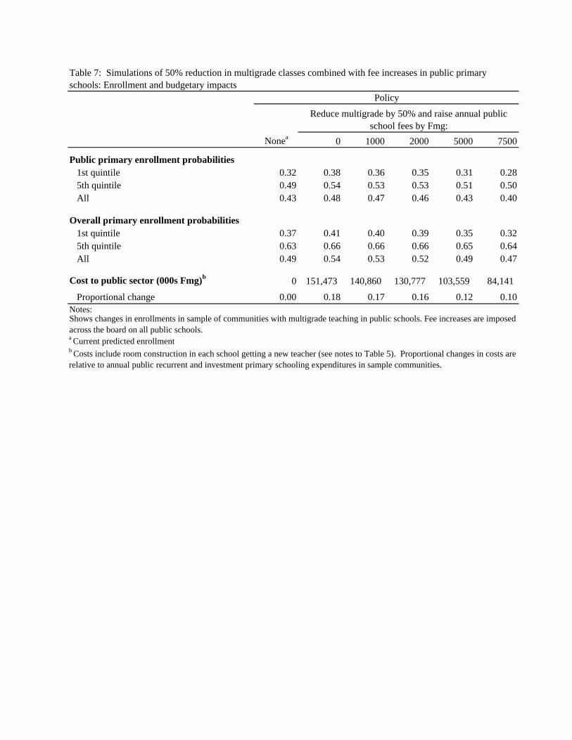
Nonea 0 1000 2000 5000 7500

Public primary enrollment probabilities1st quintile 0.32 0.38 0.36 0.35 0.31 0.285th quintile 0.49 0.54 0.53 0.53 0.51 0.50All 0.43 0.48 0.47 0.46 0.43 0.40

Overall primary enrollment probabilities1st quintile 0.37 0.41 0.40 0.39 0.35 0.325th quintile 0.63 0.66 0.66 0.66 0.65 0.64All 0.49 0.54 0.53 0.52 0.49 0.47

Cost to public sector (000s Fmg)b 0 151,473 140,860 130,777 103,559 84,141

Proportional change 0.00 0.18 0.17 0.16 0.12 0.10Notes:Shows changes in enrollments in sample of communities with multigrade teaching in public schools. Fee increases are imposed across the board on all public schools.

b Costs include room construction in each school getting a new teacher (see notes to Table 5). Proportional changes in costs are relative to annual public recurrent and investment primary schooling expenditures in sample communities.

Table 7: Simulations of 50% reduction in multigrade classes combined with fee increases in public primary schools: Enrollment and budgetary impacts

Policy

Reduce multigrade by 50% and raise annual public school fees by Fmg:

a Current predicted enrollment