The Demand for Bank Reserves and OtherMonetary Aggregates∗

Max GillmanCentral European University

Michal KejakCenter for Economic Research and Graduate Education

May 28, 2003

Abstract

The paper starts with Haslag’s (1998) model of the bank’s demandfor reserves and reformulates it with a cash-in-advance approach forboth financial intermediary and consumer. This gives a demand for abase of cash plus reserves that is not sensitive to who gets the inflationtax transfer. It extends the model to formulate a demand for demanddeposits, yielding an M1-type demand, and then includes exchangecredit, yielding anM2-type demand. Based on the comparative staticsof the model it provides an interpretation of the evidence on monetaryaggregates. This explanation relies on the nominal interest as well astechnology factors of the banking sector.

E31, E13, O42

Keywords: Bank reserves, money demand, aggregates.

∗We are grateful to participants at a seminar in CERGE-EI, Prague, and at the North-western North American Summer Econometric Society Meetings; also to Bye Jeong,Mark Harris, Sergey Slobodyan, Toni Braun, and Rowena Pecchenino, and a refereeand editor of this journal. Excellent research assistance by Szilard Benk is also appre-ciated. The first author also appreciates grant support from Central European Univer-sity. Gillman@ceu.hu, CEU, Budapest, Hungary, 36-1-327-3227, fax: 36-1-327-3232, andMichal.Kejak@cerge.cuni.cz, CERGE, Prague, Czech Republic, 420-2-2400-5186, fax: 420-2-2421-1374.

1

1 Introduction

Modeling the monetary aggregates in general equilibrium has been a chal-

lenge. There are some examples such as Chari, Jones, and Manuelli (1996),

and Gordon, Leeper, and Zha (1998), who present models that are compared

to Base money. Ireland (1995) presents one that he relates to M1-A veloc-

ity. And these models have been employed as ways to explain the actual

monetary aggregate time series evidence. However McGrattan (1998), for

example, argues that the simple linear econometric model in which velocity

depends negatively on the nominal interest rate, may do just as well or better

in explaining the evidence.

The paper here takes up the topic by modeling a nesting of the aggre-

gates that uses a set of factors that expands from the nominal interest rate

by including the production of banking services. Through this approach the

productivity factor of banking enters, as well as a cost to using money, some-

times thought of as a convenience cost that ATM machines affect. With

this general equilibrium model, and its comparative statics, an explanation

similar in spirit to McGrattan (1998), but extended to include these other

factors, is provided for the US evidence on monetary base velocity, M1 ve-

locity, and M2 velocity, as well as for the ratios of various aggregates. This

represents a more extended explanation than in previous work. And it high-

lights the limits to a nominal interest rate story, while revealing a plausible

role of technological factors in determining the aggregate mix.

The original literature on the welfare cost of inflation, well-represented

by Bailey (1992), assumes no cost to banks in increasing their exchange

services as consumers flee from currency during increasing inflations.1 The

approach builds upon the more recent literature of Gillman (1993), Aiyagari,

Braun, and Eckstein (1998), and Lucas (2000) that assumes resourse costs to

avoiding the inflation tax by using alternative exchange means. It specifies

1"The presence of the banking system has no real effect whatever but merely alters thenominal rate of inflation necessary to achieve a given real size of the government budget"(P.234, 1992); in the model here the latter statement is true, but not the former since laboris used up in banking activities, and since reserve requirements affect the real interest ratewhen there is a non-Friedman optimum rate of interest.

1

production functions of banking products that require real resources. This

gives rise to the role of technological factors in explaining the movement of

aggregates.2

The next section reviews Haslag’s (1998) model and shows how it is sen-

sitive to the distribution of the lump sum inflation proceeds. This sensi-

tivity makes tentative the growth effect of inflation with the model. The

demand for reserves can be made insensitive to the distribution of the in-

flation tax transfer by framing it within a model in which the bank must

hold money in advance as in the timing of transactions that is pioneered in

Lucas (1980). This is done in Section 3 using Haslag’s (1998) notation, Ak

production technology, and full savings intermediation. The resulting real

interest rate depends negatively on the nominal interest rate, and so infla-

tion negatively affects the growth rate, similar in fashion to the central result

of Haslag (1998). A parallel consumer cash-in-advance demand for goods is

also added, to give a model of reserves plus currency; this modeling of the

monetary base is similar to Chari, Jones, and Manuelli (1996) except that

there, as in equation (7), the inflation rate does not effect the real interest

rate.

The paper then expands the model to give a formulation of the demand for

the base plus non-interest bearing demand deposits, or an aggregate similar

to M1.3 Following a credit production approach used in a series of related

2Hicks (1935) seeks a theory of money based on marginal utility, with cash held inadvance of purchases, as Lucas (1980) follows. Hicks shunts aside both Keynes’s alterna-tive to Fisher’s quantity theory as found in his Treatise (see Gillman (2002) on flaws inthis theory), and considers "Velocities of Circulation" as in Fisher’s quantity theory an"evasion". He reasons that money use suggests the existence of a friction and that "wehave to look the friction in the face". The "most obvious sort of friction" is "the costof transfering assets from one form to another". And Hicks says that we should consider"every individual in the community as being, on a small scale, a bank. Monetary theorybecomes a sort of generalisation of banking theory." In alignment with Hicks, the agentin this paper acts as a bank in part, and the bank has costs from creating new instru-ments such as demand deposits and credit. But in contrast, here velocity is endogenouslydetermined as a fundamental part of the resulting equilibrium. And Hicks’s and Lucas’sapproaches converge with Fisher’s.

3This abstracts from the interest that is earned on some demand deposit accountsincluded in the US M1 aggregate, since this interest tends to be of nominal amountscompared to the savings accounts included in M2.

2

papers,4 the paper then adds credit, or interest bearing demand deposits, to

give a formulation for an aggregate similar to M2.

2 Sensitivity to Lump Transfers

The model starts with a demand for bank reserves that builds upon Haslag

(1998) and Chari, Jones, and Manuelli (1996). In Haslag (1998), all savings

funds are costlessly intermediated into investment by the bank. The bank

must hold reserves in the form of money. This gives rise to a bank demand

for money in order to meet reserve requirements on the savings deposits. The

consumer-agent does not use money although the lump sum inflation tax is

transferred to the agent. Instead the agent simply holds savings deposits at

the bank and earns interest as the bank intermediates all investment. The

bank’s return is lowered by the need to use money for reserves. Further,

the timing of the model is such that inflation decreases the real return to

depositors, and therefore also the growth rate, through the requirement that

reserves be held as money.

The following model gives the reported result in Haslag (1998):5

With the gross return on invested capital being 1 + A − δ, as in an Ak

model, with the time t capital stock denoted by kt, the nominal money stock

by Mt, the price level by Pt, and the net return paid on deposits denoted by

rt, the nominal profits are given as

Πt = Pt(1 +A− δ)kt +Mt−1 − Pt(1 + rt)dt. (1)

This is stated as a maximization problem with respect to kt,Mt, dt and sub-

ject to two constraints. The constraints (with equality imposed) are that the

sum of capital and last periods real balances equals deposits:

4See Gillman and Kejak (2002), Gillman, Harris, and Matyas (2003), and Gillman andNakov (2003).

5However to get this result, three changes were made to the model actually publishedin Haslag (1998), indicating incidental errors in the published paper: the money stock inthe profit equation (1) is in time t− 1, instead of t as published; and the money stock andthe price level in equation (2) are in time t− 1 instead of time t as published. The actualreturn in the paper as published is that rt = (A− δ) [1− γt (1 + gt)], where gt denotes thebalanced-path growth rate; it is independent of the inflation rate.

3

kt +Mt−1/Pt−1 = dt, (2)

and that a fraction γt−1, given in the last period, of time t deposits is held

as real money balances in time t− 1:

Mt−1/Pt−1 = γt−1dt. (3)

Assuming zero profit this yields through simple substitution the return re-

ported by Haslag (1998):

1 + rt = (1 +A− δ)(1− γt−1) + γt−1(Pt−1/Pt). (4)

The result is sensitive to who gets the lump sum cash transfer from the

government. If the transfer instead goes to the bank, the only user of money

in the model, then there is no growth effect of inflation. This can be seen

in the following way: Let the money supply process be given as in Haslag

(1998) as Mt = Mt−1 + Ht−1, where Ht−1 is the lump sum transfer by the

government. With the transfer given to the bank, the profit of equation (1)

becomes

Πt = Pt(1 +A− δ)kt +Mt−1 +Ht−1 − Pt(1 + rt)dt. (5)

Let the balanced growth rate of the economy be denoted by gt, and the

consumer’s time preference by ρ, whereby the consumer’s problem in Haslag

(1998) with log utility gives that 1+ gt = (1+ rt)/(1 + ρ). With this growth

rate in mind, the zero profit equilibrium now gives a rate of return to depos-

itors of

1 + rt = (1 +A− δ)(1− γt−1) + γt(1 + g), (6)

and there is no inflation tax on the return or on the growth rate.

Alternatively let the profit function be given as equation (5). Then as-

sume that the stock and reserve constraints, equations (2) and (3), are all in

terms of current period variables, as in a standard cash-in-advance economy

where here the reserve constraint now would look like a Clower (1967)-type

4

constraint. Then the model is exactly as in Chari, Jones, and Manuelli

(1996). This gives the result, also found in Einarsson and Marquis (2001),

that

1 + rt = (1 +A− δ)(1− γt) + γt. (7)

The return is lowered because reserves are idle but there is no inflation tax.

3 Models of Monetary Aggregates

3.1 Monetary Base

The financial intermediary has a demand for nominal money, denoted by

Mrt , as created by the need for reserves, with the reserve ratio denoted by

γ ∈ [0, 1]. But here, as in Chari, Jones, and Manuelli (1996), the reserve con-straint is considered as the bank’s Clower (1967) constraint, and structured

accordingly in a fashion parallel to the consumer’s, being that

Mrt = γPtdt. (8)

In addition the asset constraint adds together the current period real money

stock with the current period capital stock to get the current period real

deposits. In real terms this is written as

kt +M rt /Pt = dt. (9)

And the bank has to set aside cash in advance of the next period’s ac-

counting of the reserve requirement in order to meet any increase in its re-

serve requirements. The bank has revenue from its return on investment,

and costs from payment of interest to depositors, and from any increase in

money holdings for reserves.

The technology for the output of goods, as in Haslag (1998), is an Ak

production function, making the current period profit function:

Πrt = Pt(1 +A− δ)kt +Mr

t −Mrt+1 − Ptdt(1 + rt). (10)

5

The profit maximization problem is dynamic because of the way in which

money enters the bank’s profit function in two different periods, the same

dynamic feature of the consumer problem. The competitive bank discounts

the nominal profit stream by the nominal rate of interest, and maximizes

the time t discounted stream, denoted by bΠrt , with respect to the real capital

stock, kt, the real deposits, dt, and the money stock used for reserves, denoted

by Mrt , and subject to the asset stock and the Clower (1967)-type reserve

constraints of equations (8) and (9):

Maxds,Mr

s+1,ks

bΠrt =

∞Xs=t

sYi=t

µ1

1 +Ri

¶s−t{[Ps(1 +A− δ)ks (11)

+Mrs −Mr

s+1 − Ps(1 + rs)ds]

+λs [Psds −M rs − Psks]

+µs [Mrs − γPsds]} .

Assuming a constant money supply growth rate, so that the nominal

interest rate is constant over time, the first-order conditions imply that the

rate of return is

1 + rt = (1 +A− δ) (1− γ)− γRt. (12)

Using the Fisher equation of nominal interest rates (presented below), with

the above equation, shows that there is a negative effect of inflation on the

return. Combined with the consumer’s problem and the derivation of the

balanced-growth rate as depending on the real interest rate, inflation there-

fore causes a negative effect on the balanced-path growth rate.

The bank does not receive any lump sum transfer from the government;

the consumer-agent receives it all. However the distribution only affects

how much profit the intermediary makes. Since the profit is transfered to

the consumer, just as is the lump sum transfer of inflation proceeds, the

distribution of the inflation proceeds between the bank and the consumer

can be changed without affecting the allocation of resources in the economy.

For example, if the intermediary gets part of the inflation proceeds transfer,

6

by an amount at time t equal to M rt+1 −M r

t , then in equilibrium the money

terms cancel from the profit function, and Πrt/ (Ptkt) = Rt [γ/ (1− γ)] . At

the Friedman optimum, this profit is zero. 6

Consider a consumer problem as in Haslag (1998) except that now the

consumer uses cash as in Lucas (1980). The problem then includes the setting

aside of the consumer’s cash in advance of trading in the next period, denoted

by M ct+1, and the receipt of the lump sum government transfer of inflation

proceeds, denoted by Ht.

The consumer’s Clower (1967) constraint is

M ct = Ptct. (13)

The consumer also makes real (time) deposits, denoted by dt, with the

real return, denoted by rt, as the form of all savings and wholly intermediated

through banks, as in Haslag (1998). This involves choosing the next period

deposits dt+1 and receiving as real income (1 + rt) dt. The nominal current

period profit of the intermediation bank, Πrt , is received by the consumer

each period as a lump sum income source. This makes the consumer current

period budget constraint of income minus expenditures as in the following:

Pt(1 + rt)dt +Ht +Πrt +M c

t −M ct+1 − Ptct − Ptdt+1 = 0. (14)

The problem is to maximize the time preference discounted stream of

current period utility, where β ≡ 1/(1 + ρ) denotes the discount factor,

subject to the income and Clower (1967) constraints:

Maxct,dt+1,Mc

t+1

L =P∞

t=0 βt {u (ct)

+λt£Pt(1 + rt)dt +Ht +Πr

t +M ct −M c

t+1 − Ptct − Ptdt+1¤

+µt [Mct − Ptct]} .

(15)

The first-order conditions are6See Bailey (1992) for an early discussion of intermediary earnings during inflation. If

current period non-negative profit is required for the bank intermediary to exist, thena transfer to the bank as in the above-described transfer scheme, with Πrt/ (Ptkt) =Rt [γ/ (1− γ)] , would satisfy this at all inflation rates..

7

uct = λtPt(1 + µt/λt), (16)

λt/(λt+1β) = (1 + rt+1)(1 + πt+1) ≡ (1 +Rt+1), (17)

λt/(λt+1β) = 1 + µt+1/λt+1. (18)

These imply that

uct = λtPt(1 +Rt), (19)

so that the nominal interest rate is the shadow exchange cost of buying a

unit’s worth of consumption. Using this later equation to form an Euler

equation, then along the balanced-growth equilibrium with log utility it fol-

lows that the growth rate of consumption, where 1 + gt+1 = ct+1/ct, is given

by

1 + gt =1 + rt1 + ρ

. (20)

The demand for money is given by the Clower (1967) constraint, M ct =

Ptct.This standard Lucas (1980) demand function can be thought of as a

demand for “currency”, in this, the simplest version of the model. Also note

that with Pt+1/Pt ≡ 1 + πt+1, the first order condition with respect to dt

implies a Fisher-type equation whereby

1 +Rt+1 ≡ λt/(λt+1β) = (1 + πt+1)(1 + rt+1).7 (21)

The total demand for money is the sum of the bank’s and the consumer’s,

and this is set equal to the total money supply as a condition of market

clearing in equilibrium:

Mrt +M c

t =M bt . (22)

7Including the market for nominal bonds as in Lucas and Stokey (1987) would give Rt

as the price of the bonds and would explicitly derive the Fisher equation.

8

The total money supply, or market clearing, equation is that this period’s

money base, denoted by M bt plus the lump sum transfer equal next period’s

base supply of money:

M bt +Ht =M b

t+1. (23)

Assume that the money supply growth rate is constant at σ, where σ ≡Ht/M

bt .

3.2 M1

Now consider an extension in which the consumer suffers a nominal cost

of using money that is proportional to the amount of cash used to make

purchases. This can be thought of as the "convenience" cost of using money.

This can be related to the average amount stolen in robberies by pickpockets,

lost by carelessness, and spent on protection against crime and carelessness.

And, it can be Karni’s (1974) time costs or Baumol’s (1952) shoe-leather

costs. Importantly, these costs can be affected by the availability of bank

locations, and now ATM locations.8 Let this amount be given by φM ct , with

φ ∈ [0, 1). Second assume that a second bank exists, a bank that suppliesonly non-interest bearing deposits, denoted by Mdd,s

t , that can be used in

exchange. This money can be thought of demand deposits as in the US or

as a debit card as is more common in Europe. The bank charges a nominal

fee of P ddt per unit of real deposits, so that it receives from the consumer

total such receipts equal to P ddt (M

dd,st /Pt); and the bank produces these

non-interest bearing deposits through a production process. The consumer

receives from the deposit bank its nominal profit, denoted by Πddt , and the

profit from the intermediation bank, and the lump sum inflation tax transfer.

8We are indebted to Bob Lucas for originally suggesting this concept, and to RowenaPecchenino. Note that these costs are on the consumer side of the problem, while costsof alternative instruments for exchange are on the banking firm side of the problem. Theso-called shopping time costs (Lucas 2000) actually compare better to the bank firm costsin this problem, as is shown below in footnote 9. Karni’s and Baumol’s costs are a storymore about the costs on the consumer side. The diffusion of ATMs plausibly affects bothbanking productivity and the consumer’s cost of using money.

9

The consumer’s demand for the real non-interest bearing deposits is denoted

by Mddt /Pt.

The consumer chooses what fraction of purchases to be made with cash,

denoted by act ∈ [0, 1], and what fraction to be made with non-interest de-mand deposits, addt ∈ [0, 1]; where

act + addt = 1. (24)

The Clower (1967) constraints becomes

M ct = actPtct; (25)

Mddt = (1− act)Ptct. (26)

And the consumer problem now is:

Maxct,dt+1,Mc

t+1,Mddt+1,a

ct

L =P∞

t=0 βt {u (ct)

+λthPt(1 + rt)dt +Ht + bΠr

t +Πddt +M c

t +Mddt

−M ct+1 − φM c

t −Mddt+1 − (P dd

t /Pt)Mddt − Ptct − Ptdt+1

¤+µct [M

ct − actPtct]

+µddt [Mddt − (1− act)Ptct]

ª.

(27)

The first-order condition with respect to act gives that µddt = µct . In

combination with the first-order conditions with respect to the two money

stocks, M ct+1 and Mdd

t+1, this implies that

P ddt /Pt = φ. (28)

And note that the shadow cost of buying goods with cash now is given by

the marginal condition:

uct = λtPt(1 +Rt + φ), (29)

so that the shadow exchange cost now is equal to Rt + φ instead of only Rt

as in the previous subsection. The demands for the cash and for the demand

10

deposits are given by the Clower (1967) constraints in equilibrium, where the

act variable is determined by finding the equilibrium bank supply of demand

deposits and setting this equal to the demand for demand deposits.

The original bank, the capital intermediation bank, has the same prob-

lem as stated previously. Now consider the specification for the production

function of the new bank. With an bAK type production function for the

non-interest bearing demand-deposit bank, it can be shown that the equi-

librium would not be well defined. If the bA parameter equals φ, then there

is no unique equilibrium; and if bA equals any other value then there is an

equilibrium either with no demand for cash or with no demand for credit. A

unique equilibrium is satisfied by specifying a diminishing returns technol-

ogy whereby there is a margin at which the fixed φ is equal to the variable

marginal cost of producing the demand deposits. Initially assume that the

new demand deposit bank faces the following production function that is

diminishing in its capital input. Denoting the shift parameter by bAdd and

the capital input by kddt , and with α ∈ (0, 1), let the function be specified as

Mdd,st /Pt = bAdd(k

ddt )

α. (30)

With the current period profit, Πddt , given as the revenue minus the costs,

the deposit bank faces the following static profit maximization problem:

Maxkddt ,Mdd

t

Πddt = P dd

t (Mdd,st /Pt)− Ptrtk

ddt (31)

+λth bAdd(k

ddt )

α − (Mdd,st /Pt)

i.

The first-order conditions imply that

P ddt /Pt = rt/[ bAddα(k

ddt )

α−1], (32)

which when combined with the consumer’s equilibrium condition (28) gives

that

φ = rt/[ bAddα(kddt )

α−1], (33)

11

or, that

kddt = ( bAddαφ/rt)1/(1−α), (34)

which gives the supply of demand deposits as

Mdd,st /Pt = bA1/(1−α)dd (αφ/rt)

α/(1−α). (35)

As the cost of using money due to security, φ, goes to zero, the capital used

in produced non-interest bearing deposits, or debit cards, also goes to zero,

as does the output of such debit. If φ = 0, then the consumer uses only cash.

Here Mdd,st /Pt = Mdd

t /Pt and the M1 aggregate can be represented as

follows:

M ct +Mdd

t ≡M1At. (36)

The problem with this specification is that, in the equilibrium, with a

constant rate of money supply growth and a positive growth rate gt, the

ratio of M ct /M

ddt is increasing towards infinity. While there may be some

trend in this ratio empirically, this trend should be explanable by changes

in other exogenous factors that determine the ratio; with constant exoge-

nous factors, theoretically the trend should be stable on the balanced growth

path. To see that the ratio is not stable, equations (25) and (26) im-

ply that M ct /M

ddt = act/(1 − act). The solution for a

ct is found by setting

equal the supply and demand from equations (26) and (35), giving that

act = 1− [ bA1/(1−α)dd (αφ/rt)α/(1−α)]/ct, with rt = (1 +A− δ) (1− γ)− γRt − 1

by equation (12). This implies that

act/(1−act) = {1−[ bA1/(1−α)dd (αφ/rt)α/(1−α)]/ct}/{[ bA1/(1−α)dd (αφ/rt)

α/(1−α)]/ct},or

act/(1− act) = {ct/[ bA1/(1−α)dd (αφ/rt)α/(1−α)]}− 1. By inspection it is clear

that with ct rising when there is positive growth on the equilibrium path, and

with the nominal interest rate being stable given that there is a stationary

inflation rate, the ratio act/(1−act) also rises towards infinity towards a cash-

only solution with no demand deposits.

12

An alternative production function that gives a stationary ratio ofM ct /M

ddt

is one that includes an externality that affects the shift parameter bAdd. In

particular let bAdd = Addc1−αt , so that the production function is CRS in terms

of capital and goods consumption:

Mdd,st /Pt = Addct

1−α(kddt )α. (37)

This function is a type of “congestion” function that is found in the litera-

ture and that Barro and Sala-I-Martin (1995) use in the growth context for

government services. It has the property that the share of goods bought with

demand deposits, addt , is a function of the capital to goods ratio; by equations

(24), (26), and (37),

addt = Add(kddt /ct)

α. (38)

Substituting the alternative production function into the profit maximization

problem of equation (31), with bAdd = Addc1−αt , the solution is

kddt /ct = (Addαφ/rt)1/(1−α). (39)

And from equations (38) and (39), the solution for the equilibrium share of

demand deposits is

addt = A1/(1−α)dd (αφ/rt)

α/(1−α).9 (40)

With the production function of equation (37), the balanced-growth path

exists and the ratio M ct /M

ddt is stationary along it. Stationarity of M c

t /Mddt

follows directly from above where it is shown thatM ct /M

ddt = act/(1−act).By

equation (24) this can be written as M ct /M

ddt = (1− addt )/a

ddt and by inspec-

tion of equation (40) can be seen to be stationary.

9Note that if addt = 1, and so act = 0, there would be no consumer demand for cash.The monetary equilibrium would still have well-defined nominal prices as long as γ > 0,so that there was a reserves demand for cash by the intermediation bank. This could thenbe characterized solely as a “legal restrictions” demand for money. At act = 0, and γ = 0,and with a positive supply of money, prices may not be well-defined.

13

3.3 M2

The model can be expanded to its full form by allowing the agent the choice

of using costly credit to make purchases, or “exchange credit”, along with

cash or non-interest bearing demand deposits. Here the credit is like a credit

card, such as the American Express card, rather than a debit card. The

agent must pay a fee for this service that is proportional to the amount

of the exchange credit; this is like the percentage fee paid by stores using

the American Express card (without a roll-over debt feature). Denoting the

time t nominal amount of exchange credit demanded by the consumer by

M cdt , and the nominal fee by P cd

t , the consumer’s expenditure on such fees

is given by (P cdt /Pt)M

cdt .The agent also receives the nominal profit of the

exchange credit bank, denoted by Πcdt . And the consumer must pay off the

debt incurred using the exchange credit at the end of the period. But this

credit saves the agent from having to set aside money in advance of trading,

and so allows avoidance of the inflation tax. And now with three types of

exchange, let the share of consumption good purchases made by cash and by

non-interest bearing demand deposits remain notated by act and addt , and the

share of consumption good purchases made by exchange credit by acdt , where

the shares sum to one:

act + addt + acdt = 1. (41)

This adds a third Clower (1967) constraint to the consumer’s problem, al-

lowing the three constraints to be written as

M ct = Ptcta

ct , (42)

Mddt = Ptcta

ddt , (43)

M cdt = Ptct(1− act − addt ). (44)

The consumer problem now buys goods with cash or demand deposits as

before, but also has a debit of −acdt Ptct for AMEX purchases, and has a

debit of −(P ddt /Pt)M

ddt due to the AMEX fee. This makes the consumer

problem

14

Maxct,dt+1,Mc

t+1,Mddt+1,M

cdt ,act ,a

ddt

L =P∞

t=0 βt {u (ct)

+λthPt(1 + rt)dt +Ht + bΠr

t +Πddt +Πcd

t +M ct +Mdd

t −M ct+1

−φM ct −Mdd

t+1 − (P ddt /Pt)M

ddt − (P cd

t /Pt)Mcdt − Ptct − Ptdt+1

¤+µct [M

ct − actPtct]

+µddt [Mddt − addt Ptct]

+µcdt [Mcdt − (1− act − addt )Ptct]

ª.

(45)

Denote the name for the exchange credit banking firm as Amex. Amex

is assumed to supply the exchange credit, denoted by M cd,st , using only cap-

ital, denoted by kcdt , in a diminishing returns fashion similar to the technol-

ogy for the demand deposit bank. While this technology could be given as

(M cd,st /Pt) = bAcd(k

cdt )

θ,where bAcd > 0 and θ ∈ (0, 1), for a general diminish-ing returns case, the problem would arise that the equilibrium share of the

Amex credit would trend down towards zero if there was a positive growth

rate gt, making infeasible the existence of a balanced-growth path. Therefore

consider a technology similar to equation (37), which gives a stable share of

exchange credit in purchases. In particular, let the function be specified with

a congestion-type externality that affects the shift parameter bAcd, wherebybAcd = Acdc1−θ, so that

M cd,st /Pt = Acdc

1−θ(kcdt )θ. (46)

The profit maximization problem is static and given by

Maxkcdt ,Mcd

t

Πcdt = P cd

t (Mcd,st /Pt)− Ptrtk

cdt

+λthAcdc

1−θt (kcdt )

θ − (M cd,st /Pt)

i. (47)

The equilibrium conditions of the consumer and Amex bank imply that

Rt + φ = P cdt /Pt = rt/[Acdθ(k

cdt /ct)

θ−1]; (48)

kcdt /ct = [Acdθ(Rt + φ)/rt]1/(1−θ). (49)

15

This means that as the nominal interest rises the Amex bank expands credit

supply and kcdt /ct rises in equilibrium.

Equating the supply and demand for the Amex credit, from equations (44)

and (46), and using the above equation (48), the share of exchange credit

can be found to be

acdt = A1/(1−θ)cd [θ(Rt + φ)/rt]

θ/(1−θ), (50)

also rising as the nominal interest rate goes up. And note that by substitut-

ing equation (50) into equation (41), so that 1 − acdt = act + addt , and then

substituting in equation (40), the solution for act is found.10

Figure 1 illustrates the equilibrium for the credit bank. At the Friedman

optimum of R = 0, some credit would still be provided as long as φ > 0. This

use of credit at R = 0 contrasts to zero such use of credit in Gillman (1993),

Ireland (1994), and Gillman and Kejak (2002).

The money market clearing condition here is that the demand for the

exchange credit equals the supply of the exchange credit. This can also be

further aggregated to

M ct +Mdd

t +M cdt ≡M2t, (51)

and can be considered an aggregate like M2. It includes the monetary base,

demand deposits, plus the exchange credit that allows funds to interest during

the period, as do certificates of deposit, and is then paid off with“money

market mutual funds” invested in short-term government securities. So it

10Alternatively the exchange credit sector can be kept implicit by having the consumerengage in “self-production” of the exchange credit. This can be done by constrainingthe consumer’s problem by the technology constraint (46), combining this constraint withequation (44), solving for acdt , and using this to substitute in for a

cdt in the consumer

problem (45), with the consumer now choosing kcdt instead of acdt . This approach wouldmake the revised Clower contraint (44) equal to Mcd

t = PtAcdc1−θ(kcdt )θ. Setting γ = 0

and φ = 0, then Mct /(Ptct) = 1− acdt = act , and only this one Clower constraint would be

necessary. Now solve this constraint for kcdt , and it would take a form exactly analogousto a special case of the McCallum and Goodfriend (1987) shopping time constraint, but incapital instead of time, that depends on real money balances and goods in the same direc-tion: kcdt = ct[1− (Mc

t /Pt)/ct]1/θ(1/Acd)

1/θ; with ∂kcdt /∂(Mct /Pt) < 0, and ∂kcdt /∂ct > 0

(See Walsh (1998), on shopping time models.)

16

Acd(kcd/c)

Slope = r/(R+φ)

acd=Acd(kcd/c)

(acd)*

(πcd)*/[Pc(R+φ)]

(kcd/c)* kcd/c

θ

θ

Figure 1: Equilibrium in the Credit Bank Sector

is a mixed set of non-interest bearing aggregates that suffer the inflation

tax, and are traditionally thought of as money-like in nature, and of the

Amex credit and money market accounts that avoid the inflation tax, unlike

“money”.

4 Changes in Aggregates Over Time

The model of M2 can be used to analyse how subsets of aggregates change

according to changes in exogenous factors. In particular the focus is on

changes in the money supply growth, σ, or more simply in the nominal rate

of interest since this is given by R = σ + ρ. Also the focus is on changes

in the banking productivity parameters Add and Acd, and the banking cost

parameter φ. Comparative statics of these factors are then applied to explain

the actual profiles of the velocity of monetary aggregates, and the profiles of

their ratios.

17

4.1 Financial Deregulation and the Increase in BankProductivity

Significant US financial deregulation manifested with the Depository Institu-

tions Deregulation and Monetary Control Act of 1980, The Garn-St.Germain

Financial Modernization Act of 1882, the Riegle—Neal Interstate Banking and

Branching Efficiency Act of 1994, and the Gramm-Leach-Bliley Act of 1999.

The 1980 law ended phased out interest ceilings and allowed banks to pay

more interest on deposits. The 1982 law allowed banks to offer money mar-

ket accounts in order to compete with mutual funds. The 1994 act allowed

national bank branching and consolidation:

"Congress passed significant reform legislation in the 1990s. In 1994, the

Riegle—Neal Interstate Banking and Branching Efficiency Act repealed the

McFadden Act of 1927 and Douglas Amendments of 1970, which had cur-

tailed interstate banking. In particular, the McFadden Act, seeking to level

the playing field between national and state banks with respect to branch-

ing, had effectively prohibited interstate branch banking. Starting in 1997,

banks were allowed to own and operate branches in different states. This

immediately triggered a dramatic increase in mergers and acquisitions. The

banking system began to consolidate and for the first time form true na-

tional banking institutions, such as Bank of America, formed via the merger

of BankAmerica and NationsBank." (Guzman 2003).

The 1999 law permitted mergers between banks, brokerage houses, and

insurance companies, "allowing banking organizations to merge with other

types of financial institutions under a financial holding company structure"

(Hoenig 2000).

These banking deregulations can affect the model primarily by increasing

the productivity parameters in the banking sector, Acd and Add. Analyti-

cally, a proportional tax can be imposed on the banking firms, and then this

tax reduced with the advent of deregulating laws. This is equivalent to an

increase in the productivity factors.

18

4.2 Comparative Statics and Comparison to the Evi-dence

The income velocity of money is defined as income divided by a particular

monetary aggregate. The income in the economy typically is consumption

plus investment, or consumption plus savings. In the representative agent

model investment usually equals savings exactly but here there is a difference

due to the cost of intermediation. Investment plus this intermediation cost

is equal to savings, and so one way to define income is as consumption plus

savings. In the model this is c + d where d are the funds the consumer

deposits in the financial intermediary for its investment. The velocity of the

monetary aggregates can then be defined using c + d, so that the definition

of base velocity accordingly is (c+ d)/MB.

Proposition 1 Given σ > φ, and along the balanced path, the base money

velocity rises with the nominal interest rate, or ∂[(ct + dt)/MBt]/∂R > 0.

Proof. The solution for the Base velocity is(ct + dt)/MBt = [1 + (dt/ct)] /

£1− addt − acdt + γ (dt/ct)

¤, where addt =

A1/(1−α)dd (αφ/rt)

α/(1−α), acdt = A1/(1−θ)cd [θ(Rt+φ)/rt]

θ/(1−θ), rt = (A− δ) (1− γ)−γ(1 +Rt), and

dt/ct =

³1+r

−θ(1−θ)t [Acdθ(Rt+φ)]1/(1−θ)[1− φ

(R+φ)θ ]+r−α/(1−α)t (Addαφ)

1/(1−α)[1+(1/α)(σφ−1)]´

[(1+rt)ρ/(1+ρ)]+γσ.

Note that the solution of dt/ct requires substituting into the budget con-

straint of the problem in equation (45), using equations (10), (22), (23),

(31), (32), (40), (42), (43), (44), (47), (48), and (50). Assuming σ > φ,

it can be seen from inspection that, with ∂rt/∂R < 0, it must be true that

∂ (dt/ct) /R > 0. This result and inspection of the add and acd terms indicates

that ∂[(ct + dt)/MBt]/∂R > 0.

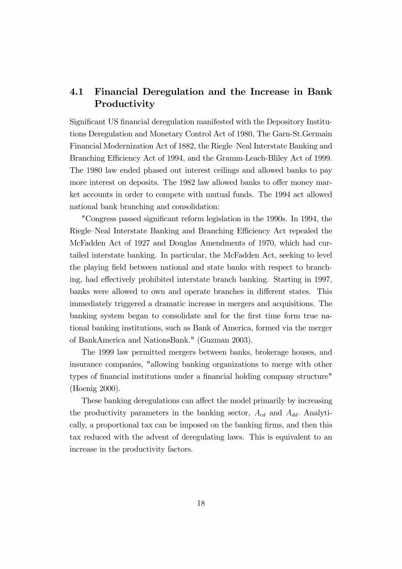
Figure 2 shows the post 1959 US base money velocity and the 10 year

bond, US Treasury, interest rate. McGrattan (1998) presents such a graph

and argues, in her comment on Gordon, Leeper, and Zha (1998), that the

nominal interest rate goes a long way to explaining base money velocity.11

11McGrattan (1998) argues that the long term rate is better to use than the short termrate that Gordon, Leeper, and Zha (1998) use. "Low frequency movements in velocity arewell-explained by low frequency movements in observed interest rates."

19

0

5

10

15

20

25

Q1 195

9

Q2 196

0

Q3 196

1

Q4 196

2

Q1 196

4

Q2 196

5

Q3 196

6

Q4 196

7

Q1 196

9

Q2 197

0

Q3 197

1

Q4 197

2

Q1 197

4

Q2 197

5

Q3 197

6

Q4 197

7

Q1 197

9

Q2 198

0

Q3 198

1

Q4 198

2

Q1 198

4

Q2 198

5

Q3 198

6

Q4 198

7

Q1 198

9

Q2 199

0

Q3 199

1

Q4 199

2

Q1 199

4

Q2 199

5

Q3 199

6

Q4 199

7

Q1 199

9

Q2 200

0

Q3 200

1

Q4 200

2

GDP/MBGOVT BOND 10Y

Figure 2: US Base Velocity and Nominal Interest Rates: 1959-2003

And this is the implication of the result of Proposition 1. The difference from

McGrattan (1998) is that she uses a simple linear econometric equation, as

found in Meltzer (1963) and Lucas (1988), to argue that the nominal interest

rate has a direct effect on velocity. Here the velocity is derived analytically

to make the point from the general equilibrium perspective.

Comparative statics for the other factors, Acd, Add, and φ, are ambiguous

in general because of the dt/ct factor, but holding dt/ct constant then all

three factor have a positive effect on base velocity. This positive direction of

the effect of these factors is also readily apparent in calibrations. While these

other factors do not provide any obvious help in interpreting base velocity

empirical evidence, they do provide an explanation as based on the model of

the evidence on the ratio of reserves to currency.

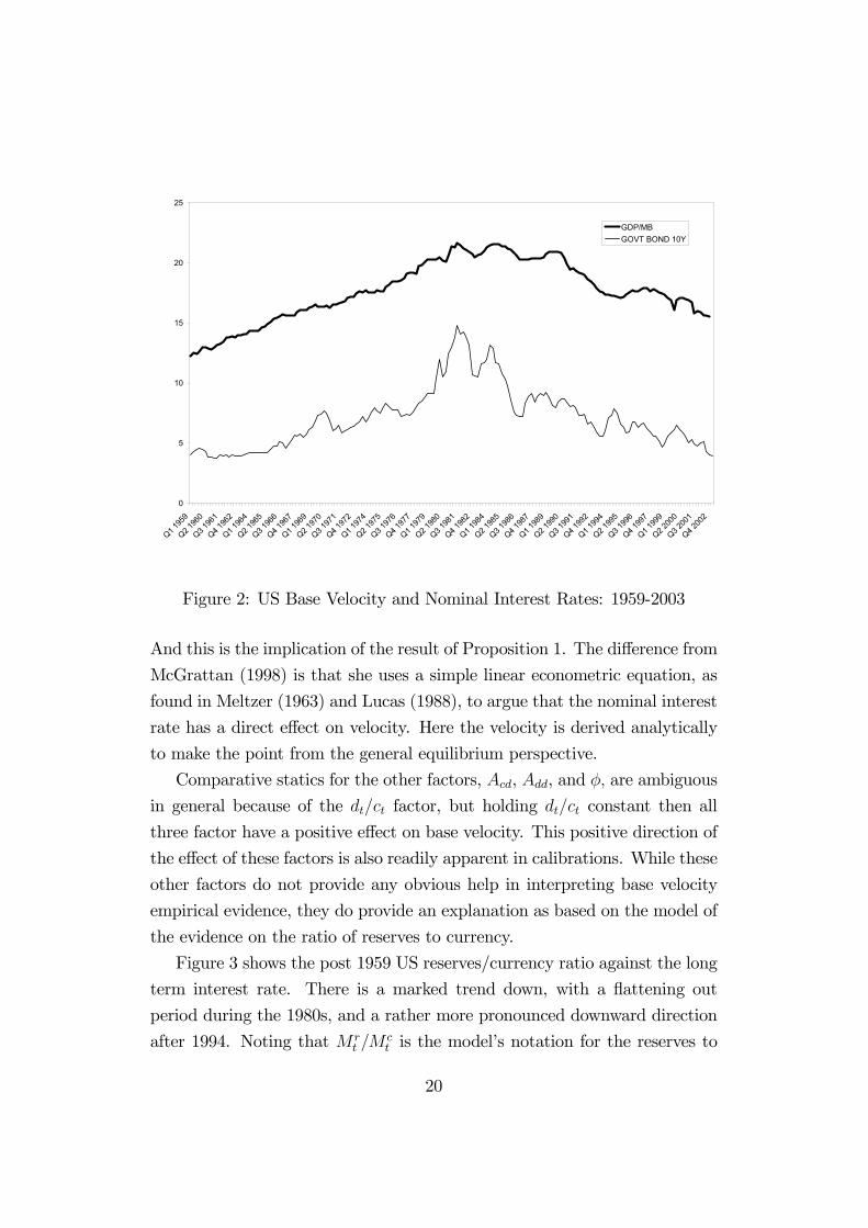
Figure 3 shows the post 1959 US reserves/currency ratio against the long

term interest rate. There is a marked trend down, with a flattening out

period during the 1980s, and a rather more pronounced downward direction

after 1994. Noting that M rt /M

ct is the model’s notation for the reserves to

20

0

2

4

6

8

10

12

14

16

Q1 195

9

Q2 196

0

Q3 196

1

Q4 196

2

Q1 196

4

Q2 196

5

Q3 196

6

Q4 196

7

Q1 196

9

Q2 197

0

Q3 197

1

Q4 197

2

Q1 197

4

Q2 197

5

Q3 197

6

Q4 197

7

Q1 197

9

Q2 198

0

Q3 198

1

Q4 198

2

Q1 198

4

Q2 198

5

Q3 198

6

Q4 198

7

Q1 198

9

Q2 199

0

Q3 199

1

Q4 199

2

Q1 199

4

Q2 199

5

Q3 199

6

Q4 199

7

Q1 199

9

Q2 200

0

Q3 200

1

Q4 200

2

Reserves/CurrencyGOVT BOND 10Y

Figure 3: US Reserves to Currency Ratio and Interest Rates: 1959-2003

currency ratio, the comparative statics are that, given σ > φ, it is unambigu-

ous that ∂(M rt /M

ct )/∂R > 0; with dt/ct held constant, ∂(M r

t /Mct )/∂φ > 0,

∂(M rt /M

ct )/∂Acd > 0, and ∂(M r

t /Mct )/∂Acd > 0. Since the US reserves/currency

trend is downward, while the effect of the nominal interest is upward in the

1959-1981 period, it appears that the nominal interest plays no role in ex-

plaining this ratio. In contrast, a downward trend in the cost of using money,

φ, serves well to explain the evidence.

Proposition 2 Given σ > φ, along the balanced growth path, M1 velocity

rises with the nominal interest rate, or ∂[(ct + dt)/M1t]/∂R > 0.

Proof. M1 velocity is defined is given by (ct+dt)/M1t = [1 + (dt/ct)] /¡1− acdt

¢.

From the proof to proposition 1, with σ > φ, then ∂ (dt/ct) /R > 0, and

with acdt = A1/(1−θ)cd [θ(Rt + φ)/rt]

θ/(1−θ), and ∂acdt /∂R > 0. It follows that

∂[(ct + dt)/M1t]/∂R > 0.

The other comparative statics are that with dt/ct constant, then an increase

in Acd and φ cause the M1 velocity to go up.

21

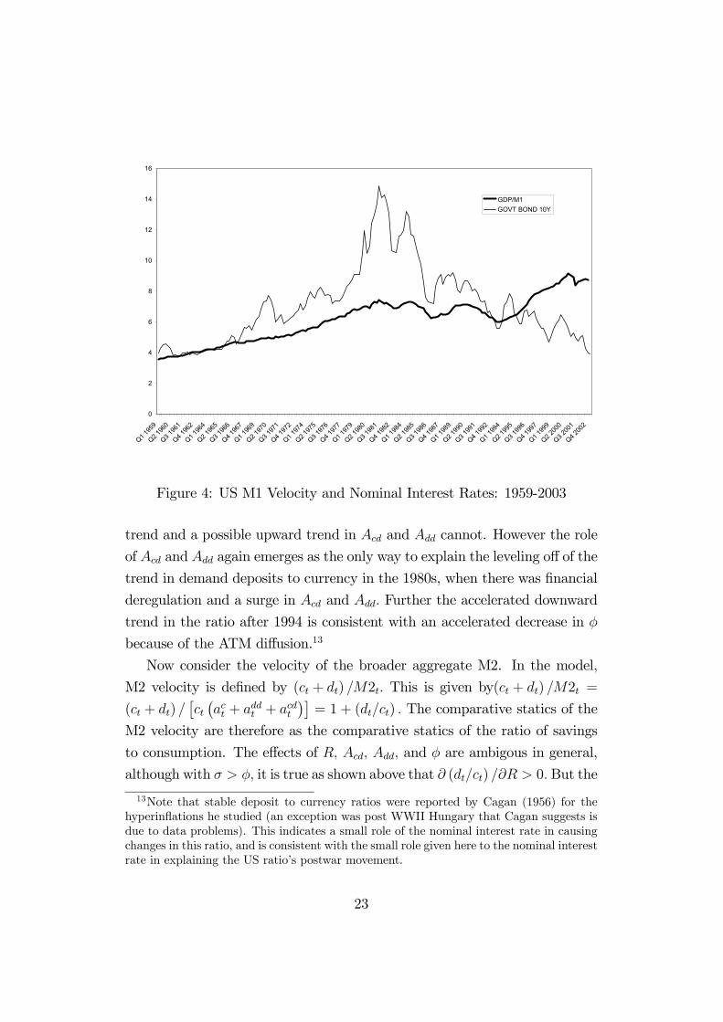
Figure 4 shows the US M1 velocity and the 10-year US Treasury interest

rate from 1959 to 2003. The rise in velocity from 1959 to 1981 is consistent

with the rise in the nominal interest rate. While still following changes in the

nominal interest rate in the 1980s, M1 velocity appears to level off rather than

fall during this period by as much as would be expected from the decrease

in the nominal interest rate. Deregulation of the 1980s, and an associated

increase in Acd presents an explanation of the leveling off of velocity in the

1980s. The striking trend upwards in velocity after 1994, as with the reserves

to currency ratio is consistent with an accelerated increase in Acd that can be

from the deregulation of interstate branching that led to national branching

and the diffusion of ATMs, as well as the banking consolidation because of

the 1999 act. Thus the two factors of the nominal interest rates and the

banking productivity each play a distinct role in this explanation.12

A way to see further into the M1 velocity profile is to look at the ratio

of its components, currency and demand deposits. Analytically the demand

deposit to currency ratio in the model is Mdd/M c. SinceMdd

Mc =A1/(1−α)dd (αφ/rt)α/(1−α)h

1−A1/(1−α)dd (αφ/rt)α/(1−α)−A1/(1−θ)cd [θ(Rt+φ)/rt]θ/(1−θ)i , the comparative stat-

ics with respect to R , Acd, Add, and φ are unambigously: ∂¡Mdd/M c

¢/∂R >

0, ∂¡Mdd/M c

¢/∂Acd > 0, ∂

¡Mdd/M c

¢/∂Add > 0, and ∂

¡Mdd/M c

¢/∂φ >

0.

Figure 5 shows the US demand deposit to currency ratio, and the 10-year

US Treasury interest rate for the same 1959-2003 period. In a first look, the

ratio simply trends down. But looking more closely shows a simple trend

down, from 1959 to 1981, that levels off in the 1980s, as with M1 velocity,

and then moves down steadily post 1994 at an accelerated rate compared to

the earlier period.

A downward trend in φ well explains the downward trend in the demand

deposit to currency ratio in a way the nominal interest rate’s pre-1981 upward

12Ireland (1995) compares US M1-A velocity with 6-month Treasury bill interest rates.He explains velocity as following a continuous upward trend due to financial innovation. Toprovide evidence on Acd, or on financial deregulation is beyond the scope of both Irelandand this paper, resulting instead in an analytic approach. However see Gillman and Otto(2002) for a paper that uses a time series on the productivity of banking to estimate amoney demand function similar to this paper’s M1 money demand.

22

0

2

4

6

8

10

12

14

16

Q1 195

9

Q2 196

0

Q3 196

1

Q4 196

2

Q1 196

4

Q2 196

5

Q3 196

6

Q4 196

7

Q1 196

9

Q2 197

0

Q3 197

1

Q4 197

2

Q1 197

4

Q2 197

5

Q3 197

6

Q4 197

7

Q1 197

9

Q2 198

0

Q3 198

1

Q4 198

2

Q1 198

4

Q2 198

5

Q3 198

6

Q4 198

7

Q1 198

9

Q2 199

0

Q3 199

1

Q4 199

2

Q1 199

4

Q2 199

5

Q3 199

6

Q4 199

7

Q1 199

9

Q2 200

0

Q3 200

1

Q4 200

2

GDP/M1GOVT BOND 10Y

Figure 4: US M1 Velocity and Nominal Interest Rates: 1959-2003

trend and a possible upward trend in Acd and Add cannot. However the role

of Acd and Add again emerges as the only way to explain the leveling off of the

trend in demand deposits to currency in the 1980s, when there was financial

deregulation and a surge in Acd and Add. Further the accelerated downward

trend in the ratio after 1994 is consistent with an accelerated decrease in φ

because of the ATM diffusion.13

Now consider the velocity of the broader aggregate M2. In the model,

M2 velocity is defined by (ct + dt) /M2t. This is given by(ct + dt) /M2t =

(ct + dt) /£ct¡act + addt + acdt

¢¤= 1 + (dt/ct) . The comparative statics of the

M2 velocity are therefore as the comparative statics of the ratio of savings

to consumption. The effects of R, Acd, Add, and φ are ambigous in general,

although with σ > φ, it is true as shown above that ∂ (dt/ct) /∂R > 0. But the

13Note that stable deposit to currency ratios were reported by Cagan (1956) for thehyperinflations he studied (an exception was post WWII Hungary that Cagan suggests isdue to data problems). This indicates a small role of the nominal interest rate in causingchanges in this ratio, and is consistent with the small role given here to the nominal interestrate in explaining the US ratio’s postwar movement.

23

0

2

4

6

8

10

12

14

16

Q1 195

9

Q2 196

0

Q3 196

1

Q4 196

2

Q1 196

4

Q2 196

5

Q3 196

6

Q4 196

7

Q1 196

9

Q2 197

0

Q3 197

1

Q4 197

2

Q1 197

4

Q2 197

5

Q3 197

6

Q4 197

7

Q1 197

9

Q2 198

0

Q3 198

1

Q4 198

2

Q1 198

4

Q2 198

5

Q3 198

6

Q4 198

7

Q1 198

9

Q2 199

0

Q3 199

1

Q4 199

2

Q1 199

4

Q2 199

5

Q3 199

6

Q4 199

7

Q1 199

9

Q2 200

0

Q3 200

1

Q4 200

2

DD/CGOVT BOND 10Y

Figure 5: US Demand Deposits to Currency Ratio and Interest Rates: 1959-2003

24

0

2

4

6

8

10

12

14

16

Q1 195

9

Q2 196

0

Q3 196

1

Q4 196

2

Q1 196

4

Q2 196

5

Q3 196

6

Q4 196

7

Q1 196

9

Q2 197

0

Q3 197

1

Q4 197

2

Q1 197

4

Q2 197

5

Q3 197

6

Q4 197

7

Q1 197

9

Q2 198

0

Q3 198

1

Q4 198

2

Q1 198

4

Q2 198

5

Q3 198

6

Q4 198

7

Q1 198

9

Q2 199

0

Q3 199

1

Q4 199

2

Q1 199

4

Q2 199

5

Q3 199

6

Q4 199

7

Q1 199

9

Q2 200

0

Q3 200

1

Q4 200

2

GDP/M2GOVT BOND 10Y

Figure 6: US M2 Velocity and Nominal Interest Rates: 1959-2003

(dt/ct) factor does not appear to play any significant role in the explanation

of base or M1 velocity. Figure 6 indeed shows that US M2 velocity has been

remarkably constant relative to the 10-year US Treasury bond rate. Thus

the explanation from the model is that the magnitude of changes in (dt/ct) ,

because of the factors considered here, is small. It is easy to confirm this

with calibrations, although this exercise is not reported. However one aspect

of this is worth noting. With a relatively unchanging dt/ct as the explanation

for a stable M2 velocity, it is internally consistent with the previous analysis

that the comparative statics of Acd , Add, and φ, with dt/ct held constant,

can be used to explain Base and M1 velocity.

Breaking down the components of M2 is more revealing. Consider the

ratio of M2 to M1. In the model this is given by

M2t/M1t = [1 + (dt/ct)] /h1−A

1/(1−θ)cd [θ(Rt + φ)/rt]

θ/(1−θ)i.

Proposition 3 Given σ > φ, along the balanced growth path, the ratio

M2t/M1t rises with an increase in the nominal interest rate, or ∂ (M2t/M1t) /∂R >

0.

25

0

2

4

6

8

10

12

14

16

Q1 195

9

Q2 196

0

Q3 196

1

Q4 196

2

Q1 196

4

Q2 196

5

Q3 196

6

Q4 196

7

Q1 196

9

Q2 197

0

Q3 197

1

Q4 197

2

Q1 197

4

Q2 197

5

Q3 197

6

Q4 197

7

Q1 197

9

Q2 198

0

Q3 198

1

Q4 198

2

Q1 198

4

Q2 198

5

Q3 198

6

Q4 198

7

Q1 198

9

Q2 199

0

Q3 199

1

Q4 199

2

Q1 199

4

Q2 199

5

Q3 199

6

Q4 199

7

Q1 199

9

Q2 200

0

Q3 200

1

Q4 200

2

M2/M1GOVT BOND 10Y

Figure 7: US Ratio of M2 to M1 and Interest Rates: 1959-2003

Proof. As shown in Proposition 1, for σ > φ, ∂ (dt/ct) /∂R > 0. And is

then clear from examination that for σ > φ, ∂ (M2t/M1t) /∂R > 0.

The other comparative statics with respect to Acd and φ are ambiguous

because of the dt/ct factor; holding dt/ct constant, the ratio M2t/M1t rises

with each of these. Now consider Figure 7, which shows the US ratio of M2

to M1 from 1959 to 2003, along with the 10-year US Treasury bond rate.

Proposition 3 provides a way to explain the upward trend in M2/M1 from

1959 to 1981, and perhaps the fall in M2/M1 from 1990 to 1994. The leveling

off of M2/M1 in the 1980s can be explained by financial deregulation and

increases in Acd; note that the downward change in R during this period,

and a downward trend in φ during this period cannot explain the leveling

off of M2/M1, as these factors work to make the ratio go down. The trend

upwards after 1994 again can be explained by upward increases inAcd because

of national branching being allowed, ATM diffusion, and consolidation.

26

5 Discussion

The demand for bank reserves that Haslag (1998) put forth helps pave the

way for modeling the demand for a range of monetary aggregates. In a

sense the Haslag (1998) model as revised here acts as the missing link that

ties together conventional money demand functions from the cash-in-advance

approach with an analogue to the monetary aggregates widely studied, by

adding a bank’s demand for cash reserves. An inflation tax on the deposit

rate of return results because, as in the cash-in-advance economies, the in-

termediation bank must in effect put aside cash-in-advance in order to meet

the demands of the reserve requirement.

Because the cash reserve requirement acts as an inflation tax on the in-

termediated investment, the model implies a type of “inverse Tobin (1965)”

effect in which inflation increases cause a decrease in the economy’s capital

stock. This effect is focused on by Stockman (1981) in which the Clower

(1967) constraint is applied to all investment. Here however, the interme-

diation bank’s Clower (1967) constraint applies only to the reserve fraction

of the investment rather than to all investment as in Stockman and so its

inverse Tobin (1965) effect is weaker.

On the basis of the intermediation bank’s demand for reserves plus the

imposition of a standard Clower (1967) constraint on the consumer’s purchase

of goods, the demand for an aggregate similar to the monetary base, reserves

plus currency (cash), is constructed whereby the inflation rate can affect the

real return to intermediated investment under an AK technology because

of the need to hold cash reserves. This model is extended to include non-

interest bearing deposits, in a way that gives an aggregate analogous to

M1. The model further is extended to include exchange credit, to give an

aggregate analogous toM2. In this fully extended model comparative statics

are presented for Base, M1 andM2 velocity, and the ratios of demand deposits

to reserves, demand deposits to currency, and M2/M1. With these analytics

the empirical evidence on the velocities and ratios are explained, requiring

more that only the nominal interest rate.

The models here enable the consumer to choose the least expensive source

27

of exchange means. As a result, the Clower (1967) constraints are not “ex-

ogenously” imposed upon the consumer but rather left as a consumer choice

to bind certain fractions of purchases to particular exchange means only to

the extent that the particular exchange means is efficient for the consumer

to use. This consumer choice amongst alternative means of exchange might

be seen as ameliorating the strength of the criticism of the “deep” models of

money that the Clower (1967) constraint is exogenously imposed, or even as

offering an alternative approach to the search for deep models.14

Note that the model of the exchange credit sets the quantity of credit

that is produced equal to the value of the output of the consumption good

that is being bought on credit. Aiyagari, Braun, and Eckstein (1998) instead

model credit as a service that is produced, and then enters as an input

into a production function for credit goods. The credit goods production is

Leontieff in its inputs of the credit service and of the value of the consumption

goods being bought with the credit. This Leontieff technology in equilibrium

implies as a special case the condition that the credit services output equals

the value of the of consumption goods being bought with the credit.15 In

the paper here, as in Gillman (1993), Ireland (1994), and Erosa and Ventura

(2000), there are no credit or cash goods per se, but only the consumption

good that can be bought with cash or credit. This in a sense can be thought of

as collapsing the Aiyagari, Braun, and Eckstein (1998) -type credit goods and

credit services into a single technology called credit, whereby the equilibrium

condition that is implied by the special case of the Leontieff technology of

Aiyagari, Braun, and Eckstein (1998) is implicitly applied.

The model’s implications for growth are that inflation lowers growth be-

cause it lowers the real interest rate, a result supported in Ahmed and Rogers

(2000). However, this feature combined with an Ak goods production tech-

nology cannot account for the substitution from effective labor to capital,

14See Bullard and Smith (2001), and Azariadis, Bullard, and Smith (2000), for example,for an alternative approach to modeling "inside" money, based on a three-period model.They apply this to anaylse the optimality of restricting inside money; Gillman (2000)analyses the optimality of such restrictions in a model similar to the paper here.15The case is that q = 1 in Aiyagari, Braun, and Eckstein (1998) model, using their

notation.

28

as induced by inflation, that Chari, Jones, and Manuelli (1996) describe

and that Gillman and Nakov (2003) further elaborate; Gillman and Nakov

(2003) find evidence in support of this substitution for the postwar US and

UK data. Thus while the Ak model provides easier analytic tractibility, a

goods production function with both labor and capital as in Gomme (1993)

and Gillman and Kejak (2002) also can account for a negative effect of infla-

tion on growth.16 And since this approach also involves the inflation-induced

labor to capital substitution, it may be useful to nest the models of monetary

aggregates within the Gomme (1993) framework.

Gillman and Kejak (2002) go partly in this direction by extending Gomme

(1993) so as to include credit, as in Section 3.3 of this paper. One advantage

of having monetary aggregates more fully embedded in the King and Rebelo

(1990)- type of endogenous growth model is that this provides the channels

by which to substitute away from inflation and so make the inflation tax

less burdonsome to the individual consumer. As Gillman and Otto (2002)

show, the Gillman and Kejak (2002) model creates an interest elasticity of

money demand that rises in magnitude with inflation. This feature also

exists in this model of this paper, and this is the central feature of the Cagan

(1956) model. Or as Martin Bailey put it "Cagan’s principal conclusion,

indeed, is that the demand for real cash balances ... has a higher and higher

elasticity at higher and higher rates of inflation" (Bailey 1992). And Mark

and Sul (2002) report recent international panel evidence in support of the

Cagan (1956) money demand function. Only with such an elasticity, within

the general equilibrium money demand function, are Gillman, Harris, and

Matyas (2003) able to show that they can explain international evidence on

inflation and growth.17

16See also Jones and Manuelli (1995).17Paal and Smith (2000) offer an overlapping generations model in which low inflation

can cause a positive effect on growth, while higher inflation causes a negative level. Thisis supported in the panel evidence of Ghosh and Phillips (1998), Khan and Senhadji(2000), Judson and Orphanides (1996), and Gillman, Harris, and Matyas (2003) in whicha threshold level of inflation is found after which the inflation-growth effect is negative.However the positive effect at low inflation rates is found to be insignificant in these papers.And Gillman, Harris, and Matyas (2003) show that using instrumental variables, the effectof inflation on growth is negative for all positive levels of inflation, across both OECD andAPEC regions, as well as in the full sample; Ghosh and Phillips (1998) also find this for

29

References

Ahmed, S., and J. H. Rogers (2000): “Inflation and the Great Ratios:

Long Term Evidence from the US„” Journal of Monetary Economics,

45(1), 3—36.

Aiyagari, S. R., R. A. Braun, and Z. Eckstein (1998): “Transaction

Services, Inflation, and Welfare,” Journal of Political Economy, 106(6),

1274—1301.

Azariadis, C., J. Bullard, and B. Smith (2000): “Private and Public

Circulating Liabilities,” Manuscript.

Bailey, M. (1992): “The Welfare Cost of Inflationary Finance,” in Stud-

ies in Positive and Normative Economics, Economists of the Twentieth

Century, chap. 15, pp. 223—240. Edward Elgar, Reprinted from Journal of

Political Economy (April 1956) 64(2):93-110.

Barro, R., and X. Sala-I-Martin (1995): Economic Growth. McGraw-

Hill, Inc., New York.

Baumol, W. J. (1952): “The Transactions Demand for Cash: An Inventory

-Theoretic Approach,” 66, 545—66.

Bullard, J., and B. Smith (2001): “The Value of Inside and Outside

Money,” Working Paper 2000-027C, The Federal Reserve Bank of St.

Louis.

Cagan, P. (1956): “The Monetary Dynamics of Hyperinflation,” in Studies

in the Quantity Theory of Money, ed. by M. Friedman, pp. 25—120. The

University of Chicago Press, Chicago.

Chari, V., L. E. Jones, and R. E. Manuelli (1996): “Inflation, Growth,

and Financial Intermediation,” Federal Reserve Bank of St. Louis Review,

78(3).

a full sample.

30

Clower, R. (1967): “A Reconsideration of the Microfoundations of Mone-

tary Theory,” Western Economic Journal, 6(1), 1—9.

Einarsson, T., and M. H. Marquis (2001): “Bank Intermediation Over

the Business Cycle,” Journal of Money, Credit and Banking, 33(4), 876—

899.

Erosa, M., and M. Ventura (2000): “On Inflation as a Regressive Con-

sumption Tax,” University of Western Ontario Department of Economics

Working Papers 20001 (RePEc:uwo:uwowop:20001).

Ghosh, A., and S. Phillips (1998): “Inflation, Disinflation and Growth,”

IMF Working Paper WP/98/68, International Monetary Fund.

Gillman, M. (1993): “Welfare Cost of Inflation in a Cash-in-Advance Econ-

omy with Costly Credit,” Journal of Monetary Economics, 31, 22—42.

(2000): “On the Optimality of Restricting Credit: Inflation-

Avoidance and Productivity,” Japanese Economic Review, 51(3), 375—390.

(2002): “Keynes’s Treatise: Aggregate Price Theory for Modern

Analysis,” European Journal of the History of Economic Thought, 9(3),

430—451.

Gillman, M., M. Harris, and L. Matyas (2003): “Inflation and Growth:

Explaining a Negative Effect,” Empirical Economics, Forthcoming.

Gillman, M., and M. Kejak (2002): “Modeling the Effect of Inflation:

Growth, Levels, and Tobin,” in Proceedings of the 2002 North American

Summer Meetings of the Econometric Society: Money, ed. by D. Levine.

http://www.dklevine.com/proceedings/money.htm.

Gillman, M., and A. Nakov (2003): “A Revised Tobin Effect from Infla-

tion: Relative Input Price and Capital Ratio Realignments, US and UK,

1959-1999,” Economica, Forthcoming.

31

Gillman, M., and G. Otto (2002): “Money Demand: Cash-in-

Advance Meets Shopping Time,” Department of Economics Working Pa-

per WP03/02, Central European University, Budapest.

Gomme, P. (1993): “Money and Growth: Revisited,” Journal of Monetary

Economics, 32, 51—77.

Gordon, D., E. Leeper, and T. Zha (1998): “Trends in Velocity and Pol-

icy Expectations,” Carnegie-Rochester Conference Series on Public Policy,

49, 265—304.

Guzman, M. (2003): “Slow But Steady Progress Toward Financial Deregu-

lation,” Southwest Economy 1, Federal Reserve Bank of Dallas.

Haslag, J. H. (1998): “Monetary Policy, Banking, and Growth,” Economic

Inquiry, 36, 489—500.

Hicks, J. (1935): “A Suggestion for Simplifying the Theory of Money,”

Economica, 2(5), 1—19.

Hoenig, T. (2000): “Discussion of "The Australian Financial System in the

1990s",” inThe Australian Economy in the 1990s: Conference Proceedings.

Reserve Bank of Australia.

Ireland, P. (1994): “Money and Growth: An Alternative Approach,”

American Economic Review, 55, 1—14.

(1995): “Endogenous Financial Innovation and the Demand for

Money,” Journal of Money, Credit and Banking, 27(1), 107—123.

Jones, L., and R. Manuelli (1995): “Growth and the Effects of Inflation,”

Journal of Economic Dynamics and Control, 19, 1405—1428.

Judson, R., and A. Orphanides (1996): “Inflation, Volatility and

Growth,” Board of Governors of the Federal Reserve System Finance and

Economics Discussion Series, 96(19).

32

Karni, E. (1974): “The Value of Time and Demand for Money,” Journal of

Money. Credit and Banking, 6, 45—64.

Khan, M. S., and A. S. Senhadji (2000): “Threshold Effects in the Re-

lationship Between Inflation and Growth,” IMF Working Paper.

King, R. G., and S. Rebelo (1990): “Public Policy and Economic Growth:

Deriving Neoclassical Implications,” Journal of Political Economy, 98(3),

S126—S150.

Lucas, Jr., R. E. (1980): “Equilibrium in a Pure Currency Economy,”

Economic Inquiry, 43, 203—220.

(1988): “Money Demand in the United States: A Quantitative

Review,” Carnegie-Rochester Conference Series on Public Policy, 29, 169—

172.

(2000): “Inflation and Welfare,” Econometrica, 68(2), 247—275.

Lucas, Jr., R. E., and N. L. Stokey (1987): “Money and Interest in a

Cash-in-Advance Economy,” Econometrica, 55, 491—513.

Mark, N., and D. Sul (2002): “Cointegration Vector Estimation by Panel

DOLS and Long Run Money Demand,” Technical Working Paper 287,

National Bureau of Economic Research, Cambridge, MA.

McCallum, B. T., and M. S. Goodfriend (1987): “Demand for Money:

Theoretical Studies,” in New Palgrave Money, ed. by M. J. Eatwell, and

P.Newman. Macmillan Press, New York.

McGrattan, E. (1998): “Trends in Velocity and Policy Expectations: A

Comment,” Carnegie-Rochester Conference Series on Public Policy, 49,

305—316.

Meltzer, A. (1963): “The Demand for Money: The Evidence from the

Time Series,” Journal of Political Economy, 71, 219—246.

33

Paal, B., and B. Smith (2000): “The Sub-Optimality of the Friedman Rule

and the Optimum Quantity of Money,” Manuscript, Stanford University.

Stockman, A. (1981): “Anticipated Inflation and the Capital Stock in a

Cash-in-Advance Economy,” Journal of Monetary Economics, 8(3), 387—

393.

Tobin, J. (1965): “Money and Economic Growth,” Econometrica, 33(4,

part 2), 671—684.

Walsh, C. E. (1998): Monetary Theory and Policy. The MIT Press, Cam-

bridge, MA.

34