The Demand for and the Supply of Distribution Services: A Basis for the Analysis of Customer Satisfaction in Retailing

by Roger R. Betancourt* Monica Cortiñas** Margarita Elorz** Jose Miguel Mugica**

* Department of Economics, U. of Maryland, College Pk., MD and AffiliateFaculty, Department of Marketing, R. H. Smith School of Business, U. ofMaryland. ** Departamento de Gestion de Empresas, Universidad Publica deNavarra, Campus de Arrosadia, 31006 Pamplona (Navarra) Spain.

The Demand for and the Supply of Distribution Services: A Basis for the Analysis ofCustomer Satisfaction in Retailing.

Abstract:

This paper brings together two bodies of literature. One of them is a literature on the special roleof the consumer in retailing. The other one is the literature on customer satisfaction. This joiningof literatures is accomplished by identifying distribution services as outputs of retail firms andfixed inputs into the production functions of consumers. The result is a new conceptualframework for the analysis of customer satisfaction in retailing. Implementation of thisframework with supermarket data shows that the five main categories of distribution servicesidentified by the conceptual framework are economically important and statistically robustdeterminants of customer satisfaction with supermarkets. These results are obtained controllingfor other variables typical of the customer satisfaction literature and measuring customersatisfaction in a manner consistent with that literature. Perhaps our most interesting result is thatthe effect of the determinants of customer satisfaction on future purchase intentions in thesupermarket case is different when measured directly than when measured indirectly through theattributes/satisfaction/ purchase intentions chain.

Keywords: Retailing; Customer Satisfaction; Distribution Services; Supermarkets.

JEL Code: M3; L8; M31; L81.

1. Introduction

1

In this paper, we bring together two separate bodies of literature. First, we consider the

main strand of literature on customer satisfaction. This strand is best illustrated by Anderson and

Sullivan’s (1993) frequently cited paper. The latter focuses on the manufacturer’s point of view

and the firm as the unit of analysis, stresses the quality of products relative to expectations about

that quality as the main determinant of customer satisfaction, and emphasizes repurchase

intentions as the relevant economic performance variable determined by satisfaction.

Subsequent work has taken a number of directions. One sub-strand has considered the

impact of customer satisfaction on other performance variables. For instance, Anderson, Fornell

and Lehman (1994) emphasize the rate of return on investment and Anderson, Fornell and

Mazvancheryl (2004) emphasize Tobin’s q as the relevant performance variable. Given the

nature of our data, we can obtain direct results on the relation between attributes and customer

satisfaction and between customer satisfaction and repeat patronage intentions but we can only

obtain results with respect to other economic performance variables by making extraneous

assumptions about behavior.

A related sub-strand of literature has proceeded by extending these ideas to the service

sector. In some cases this is done treating “... service quality and customer satisfaction almost

interchangeably...”, Rust and Zahoric (1993, p.193), and in other cases differentiating between

these two concepts. For example Gomez, Mclaughlin and Wittink (2003), who focus on the firm

in food retailing, reduce 18 attributes identified by survey questions into three components

[customer service, quality and value] through the use of factor analysis. It is these components

that are assumed to determine satisfaction. Malthouse, et.al (2004) extend the analysis of

customer satisfaction to multiple units of a service sector firm and apply it to the health and

2

newspaper industries. Our approach provides an explicit and close relationship between service

quality and customer satisfaction in retailing in general and focuses on the establishment rather

than the firm.

Yet another related sub-strand of this literature emphasizes asymmetries and non-

linearities in the links between attributes satisfaction and economic performance variables, for

example Anderson and Mittal (2000). With cross-section data we will not be able to say

anything about asymmetries, but we are able to address an important non-linearity that affects

whether one employs the direct or the indirect approach to evaluate effects on performance. If

the links were linear the direct impact of attributes on economic performance variables would be

the same as the indirect one and either approach is valid. An example of the use of the direct

approach in the case of retention is Rust and Zahoric (1993). The indirect approach is obtained

by first estimating the impact of an attribute on customer satisfaction and subsequently

estimating the impact of customer satisfaction on the economic performance variable. An

example of the use of the indirect approach is Kamakura, et.al (2002). We show that in the

context of our data the indirect and the direct approach generate different answers.

We extend these ideas to the retail sector by providing a new conceptual framework for

the analysis of customer satisfaction in retailing. This framework provides an answer to two

difficult questions not addressed explicitly in the customer satisfaction literature. First, since

retailing is a multi-product activity, what is the relevant product quality in retailing? Second,

what are the relevant quality expectations in the case of retailing?

A second and separate body of literature on the role of the consumer in retailing exists

and is relevant for our purposes. This literature has argued that retailing differs from other

3

industries in that the consumer plays a different role. For instance, Oi (1992) identifies this

difference by arguing that self-service implies that the consumer is an input in the transformation

process in retailing. Shaw, Nisbet and Dawson (1989) identified this difference by arguing that

demand and marketing forces determine establishment (store) size, instead of economies of scale

as in other industries. Ofer (1973) argues that the store has two outputs and identifies the main

difference characterizing retailing as the result of the consumer choosing the ratio of the two

outputs. Finally, Berne, Mugica and Yague (1999) argue that the difference from other

industries is that the store’s output is the result of an encounter between the consumer and the

retailer.

The new conceptual framework for the analysis of costumer satisfaction put forth here,

which is based on Betancourt (2004), incorporates these arguments. Furthermore, it will be

shown how the various roles of the consumer in retailing identified in this literature can be

captured with a proper of specification of the demand for and the supply of distribution services.

This is done in the next section where these distribution services are also described in detail.

In section III we discuss a variety of estimation issues. The latter include the

specification of our estimating equation, the choice of estimation method, and unique

characteristics of our data and measurement of distribution services. In section IV we present

the main results of employing our approach to estimate the determinants of customer satisfaction

in supermarkets with a particular body of cross-section data. In Section V we present the results

of estimating the effects of distribution services on repeat patronage intentions directly and

indirectly through their effect on customer satisfaction. We also draw here the managerial

implications of our results. A brief conclusion highlights the main contributions and limitations

4

that suggest areas for further research. A data appendix, available upon request, provides

additional details on the nature of our data.

2. Conceptual Framework

Betancourt (2004) provides the tools to reconcile different views on the role of the

consumer in retailing. This can be done by drawing the implications of a proper specification of

distribution services as outputs of retail firms and fixed inputs into household production

functions of consumers. This is the first task of this section. More importantly, however, this

reconciliation provides the conceptual framework for linking customer satisfaction with the store

to the demand and supply of turnover and distribution services. This link, which is also

explicitly drawn in this section, is one of the main contributions of this paper.

Distribution services have been identified as outputs in the retail literature by various

authors, starting with Bucklin (1973 ) and continuing with Betancourt and Gautschi (1988 ) and

Oi (1992) among others. Usually they can be assigned to one of the following five broad

categories: accessibility of location, information, assortment (breadth or depth), assurance of

product delivery (in the desired form or at the desired time), and ambiance. Attempts at

measurement of these services at the level of the store are starting to appear, e.g., Barber and

Tietje (2004), and will be explicitly discussed in the next section.

Here, we note the essence of the process whereby the level of distribution services

provided by a store is determined. Namely, as a result of how equilibrium in a retail market

comes about. The retailer sets a level of services, the consumer responds to that level of services

by choosing what quantities to buy and how frequently to patronize the store. In the end stores

that don’t provide an adequate bundle of services to a segment of a market get no patronage and

5

go out of business. Since this is a market equilibrium outcome, it is sometimes difficult to

visualize.1

In order to proceed, it is necessary to capture the role of distribution services as outputs of

retailers. This will be done through the specification of the cost function of the retailer as

C = C (v, Qs , Ds ), (1)

where v are the prices of the inputs of the retailers other than goods sold, Qs is a vector of the

levels of output of retail items supplied by the retailer, Ds is a vector of the levels of distribution

services supplied by the retailer and C are the costs of retailing net of the costs of goods sold.2

Similarly, it is necessary to capture the role of distribution services as fixed inputs into the

household production functions of consumers. This is done through the specification of the

demand function for retail items as

Qd = f (p, Ds , W), (2)

where Qd is a vector of the quantity of retail items demanded by consumers, p are the prices of

these retail items, Ds is a vector of the levels of distribution services provided to consumers at a

retailer and W is the level of wealth.3

Betancourt (2004, Ch.4) shows that Oi’s argument about the consumer as an input into the

production function collapses to acknowledging that distribution services are outputs of the

retailer, as in (1), and that they influence the demand functions of consumers, as in (2). In a

market equilibrium, where turnover demand (Qd ) equals turnover supply (Qs ) = Q, Oi’s

argument on the special role of the consumer reduces to acknowledging the endogeneity of Q and

Ds in any econometric procedure.

Betancourt’s specification of the store’s outputs (2004, Ch.4) is consistent with Ofer’s

6

argument that the store output has at least two dimensions: the level of turnover (Qs) and the level

of distribution services (Ds). Hence, Ofer’s argument is easily captured in this framework. That

is, the quantities of retail items demanded by the consumer, Qd , are specified as a function of

retail prices and the actual distribution services provided by the store, Ds. By choosing Qd, the

consumer chooses the ratio between Qd and Ds as well, which was one of Ofer’s assertions.

Shaw, Nisbet and Dawson’s argument is not addressed in detail by Betancourt (2004) but

can be easily accommodated in this framework. In the short-run store size and the supply of retail

items and distribution services [Qs; Ds ] provided by the store is relatively fixed and determined

by the retailer; in the long-run, however, demand and marketing forces [Qd ; Dd ] are likely to be

more important as emphasized by Shaw, Nisbet and Dawson. That is higher levels of these

variables [Qd (H); Dd (H)] due to demographic, economic or technological changes, for example,

will induce the building of larger stores and the provision of higher levels of turnover and

distribution services by the retailer [Qs = Qd (H); Ds = Dd (H)].

Finally, Berne, Mugica and Yague’s argument can be reconciled with this framework as

follows: the outcome of the encounter between the retailer and the customer is a relation between

the quantities demanded of these two types of output [Qd ;Dd ] and the quantities supplied of these

two types of output [Qs ; Ds ]. One would expect this relation normally to satisfy these

inequalities, Qd #Qs and Dd $ Ds . The first inequality rules out consumers facing stock-outs for

any one item and the second inequality rules out retailers providing services that are not wanted

by consumers for any one service. This conceptualization generates four possible cases.

A relatively simple one assumes that as a result of the encounter both equalities hold. In

this case all the analyst has to worry about is the econometric problem of endogeneity of Q = Qd

7

= Qs and D = Dd = Ds . Another relatively simple case assumes no capacity limitations (Qd < Qs

) and that quantities demanded of distribution services equal quantities supplied, i.e., [ Dd = Ds ],

that is the outcome of this encounter is a fully satisfied customer. In this case customer

satisfaction is at its maximum and, if this is the case for every customer, its measurement is

irrelevant. To our knowledge, this economic interpretation of the limit condition has not been

identified in the prior literature on customer satisfaction in retailing.

The third and most interesting case, in our context, is one where there are no capacity

limitations (Qd < Qs ) and consumers’ demand for at least one distribution service is always

greater than the level supplied by the retailer, Dd > Ds. It is in this case that the measurement of

customer satisfaction becomes intrinsically meaningful, since a consumer may be very close or

very far from its desired or demanded level of distribution services. Furthermore, the distance

between the demand and supply of distribution services, Dd - Ds , suggests itself as a natural

measure of the lack of customer satisfaction. This conceptual foundation for the measurement of

customer satisfaction in retailing is one of our principal contributions to the literature.

Incidentally, the no capacity limitations condition [Qd < Qs ] is necessary for the degree of

consumer satisfaction to be economically interesting. Because it allows the retailer a mechanism

to satisfy increased demand by customers, which is what generates profits from increasing

customer satisfaction.4

Since identification of this case is one of the main contributions of this paper to the

literature, it is useful to add precision to the discussion as follows: consumer i satisfaction with a

store, k, is going to be given by a relation of the following form

Si (k) = f{ [Dd (i) - Ds (k)]j , p(k), Z(i, k)}, (3)

8

where Si (k) is a measure of customer satisfaction, i.e., of consumer i satisfaction with store k.

This satisfaction is going to be a decreasing function, fj’< 0, of the distance between each of the j

distribution services actually provided by store k, Ds (k), and the level of each of the j distribution

services demanded by consumer i, Dd ( i ).

Thus, in the context of retailing the emphasis on product quality in the customer

satisfaction literature is captured by the emphasis on distribution services provided by the retailer,

Ds (k), and the emphasis on expectations is captured by the level of distribution services

demanded by consumers, Dd (i). Once again the establishment of these correspondences is absent

from the literature on customer satisfaction in retailing. None of the references cited in the

introduction addresses these two issues explicitly. Implicitly, Gomez, McLaughlin and Wittink

(2003) addressed the first one by labeling a subset of the attributes in one of their three factors

quality. But, these attributes leave out a substantial number of products available in the store and

include a few but by no means all services. Similar issues arise in the food retailing literature on

this topic cited by these authors. The specification of the rest of the items in (3 ) is less

innovative and follows the literature. Namely, one would also expect the function in (3) to be a

decreasing function of the average prices charged by store k. In addition, consumer characteristics

or other store characteristics may affect the consumer’s satisfaction with a store and are captured

by the vector Z(i , k). Both of these ideas are expressed, for example, in Gomez, Mclaughlin and

Wittink (2003).

In sum, equation (3) incorporates the original ideas of the literature on customer

satisfaction and the literature on the role of the consumer in retailing while relying on widely

accepted fundamental economic concepts.

9

3. Empirical Implementation: Estimation and Data Issues

Equation (3) represents the most general statement of the relationship between customer

satisfaction and the concepts that correspond to product quality and expectations in the typical

retail setting. It can allow for asymmetries and nonlinearities in the relation through the

specification of the function f. Furthermore, it can be viewed as a stand alone relation or as the

customer satisfaction module in a more general setting where the aim is to implement the service

profit chain framework or the return to quality framework or any variant of these frameworks.

How one proceeds with respect to these issues is determined to some extent by the nature

of the data available.5 For instance, if only cross-section data are available asymmetries can not

be captured but non-linearities can be. Similarly, if the data available are on establishments rather

than firms one can estimate the stand alone relation but not many of the variants that require a

module linked directly to economic performance variables, which usually refer to firms. In our

case we are able to estimate directly the impact of customer satisfaction on repeat patronage

intentions, which some may call predictions of future loyalty. We will discuss this issue in

Section V.

In general one does not observe the level of distribution services demanded by consumers,

Dd (i). Nonetheless, in principle the demand for these distribution services can be estimated. For

example, by constructing surveys similar to what already exist but asking different questions.6 A

simpler alternative is to assume consumers are never satisfied and that they always demand the

maximum level of demand they can expect with respect to any distribution service. This

expectation leads to the demand for each of the j distribution services set at its maximum, Dd (i) =

M. When the latter is assumed the same for all consumers and distribution services, one can

10

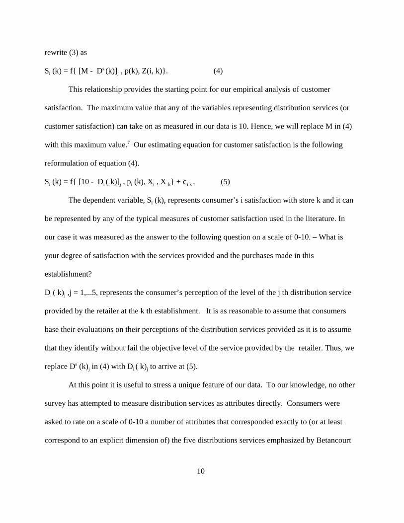
rewrite (3) as

Si (k) = f{ [M - Ds (k)]j , p(k), Z(i, k)}. (4)

This relationship provides the starting point for our empirical analysis of customer

satisfaction. The maximum value that any of the variables representing distribution services (or

customer satisfaction) can take on as measured in our data is 10. Hence, we will replace M in (4)

with this maximum value.7 Our estimating equation for customer satisfaction is the following

reformulation of equation (4).

Si (k) = f{ [10 - Di ( k)]j , pi (k), Xi , X k} + ,i k . (5)

The dependent variable, Si (k), represents consumer’s i satisfaction with store k and it can

be represented by any of the typical measures of customer satisfaction used in the literature. In

our case it was measured as the answer to the following question on a scale of 0-10. – What is

your degree of satisfaction with the services provided and the purchases made in this

establishment?

Di ( k)j ,j = 1,...5, represents the consumer’s perception of the level of the j th distribution service

provided by the retailer at the k th establishment. It is as reasonable to assume that consumers

base their evaluations on their perceptions of the distribution services provided as it is to assume

that they identify without fail the objective level of the service provided by the retailer. Thus, we

replace Ds (k)j in (4) with Di ( k)j to arrive at (5).

At this point it is useful to stress a unique feature of our data. To our knowledge, no other

survey has attempted to measure distribution services as attributes directly. Consumers were

asked to rate on a scale of 0-10 a number of attributes that corresponded exactly to (or at least

correspond to an explicit dimension of) the five distributions services emphasized by Betancourt

11

and Gautschi (1988). With respect to four of them, there seems to be a one to one relation

between the distribution service and the measured attribute.8

That is, accessibility of location, Di (k)1 , is measured from the answer to the question – To

what extent the store’s location facilitates your patronizing and accessibility to the retail

establishment? Information, Di (k)2 , is measured from the answer to the question – To what extent

the employees and the signs in this establishment facilitate your information needs with respect to

items, their location in the store, prices, sales, etc.? Assortment, Di (k)3, is measured

from the answer to the question – To what extent the assortment and variety in the store products

facilitate your making all your purchases at this establishment? Finally, ambiance, Di (k)5 , is

measured from the answer to the question – To what extent your treatment by employees, and the

cleanliness and orderliness of the store allow your purchases to be an agreeable experience?

With respect to the last distribution service, assurance of product delivery (Di (k)4 ), the

situation differs in two ways. First, it has at least two dimensions, desired form and desired time.

Second, in the data there were two questions that picked up different aspects of assurance of

product delivery at the desired time. Our approach was to use the simple average of the answers

to the following two questions – To what extent the number of registers open and the acceptance

of different means of payment facilitate the speed and convenience of paying for your purchases?;

To what extent the hours and the days the store is open facilitate making your purchases when

you need to do so?

Notice that the interpretation of the effects of any of these five variables on customer

satisfaction remains the same. That is, an increase in [10 - Di ( k)j ] implies a lowering of the

level of the j th distribution service as perceived by the consumer and, thus, it should result in a

12

lower level of customer satisfaction because the distance between the quality or service offered

and the one expected has increased. Just as noted earlier (note 7) this interpretation is at best

implicit in the references in the literature. Also note that there was a similarly rated question on

store prices, pi (k) = Xi (k)6. Namely, – To what extent the prices in the store are high relative to

other similar establishments?

Before proceeding it is useful to characterize the nature of the data in more general terms.

The data base for this study is a survey of consumers at various supermarkets in Pamplona carried

out in 1998. Traditional stores or hypermarkets were not included in the survey.9 Eleven

supermarkets were selected to have their customers interviewed. These supermarkets belonged to

seven different firms and there were four firms that each had two supermarkets in our selected

set.10 A total of 874 usable customer questionnaires were generated from these interviews: the

maximum number of interviews from any one supermarket was 85 and the corresponding

minimum number was 79. Thus, the total number of consumers was fairly evenly divided across

the eleven supermarkets.11

In implementing equation (5) empirically we selected a number of variables for inclusion

as explanatory variables for various reasons. For instance, general demographic characteristics of

consumers were included as controls, but we had no expectations as to how gender (Xi 7),age ( Xi 8

), position in the life cycle ( Xi 9 ) or extent of work outside the home (Xi 10 ) would affect

customer satisfaction.12 Two objective characteristics of customers buying habits were also

included as controls. These were the length of stay at the store (Xi 11 ) and the size of the market

basket (Xi 12). On the other hand, a third characteristic of customers buying habits, the frequency

of purchases at this establishment within a month (Xi 13 ), was initially excluded given that we

13

were not focusing on cumulative customer satisfaction.

Attitudes toward purchasing food products were captured in six variables. The first three

capture attitudes toward purchasing food products that are relevant for any establishment; the last

three capture attitudes relevant for the particular establishment patronized by the consumer. The

former were: do you enjoy engaging in this activity by yourself (Xi 14 ); how important is the time

you spent on this activity (Xi 15 ); and do you search for alternative establishments while engaged

in this activity (Xi 16 ). The latter were: at this establishment do you ask for help from employees

(Xi 17 ), for delivery services to your home (Xi 18 ), or for someone to accompany you shopping

(Xi 19 ). After some experimentation, which showed they made little difference to the results, we

decided to exclude these last three variables from the empirical analysis. Two variables that

capture objective characteristics of the environment were included: namely, surface area [ X 22 (k)]

to capture the effect of store size and dummies for the firm to which the store belongs, F (k), to

capture firm effects.

One econometric problem that arises in estimating equation (5) is that our dependent

variable can be interpreted as censored at the top and at the bottom.13 The standard procedure to

address censoring is Tobit analysis. In our case, however, it is not clear that the censoring

interpretation applies.14 Indeed the analysis leading to our estimating equation suggests that 10 is

a true maximum. If we assume that 0 is a true minimum, there is no censoring. Incidentally the

problem is also mitigated in our case by the fact that many of our variables are measured on the

same scale as the dependent one. Finally, the assumption of homoskedasticity is likely to be

violated in our case (since our observations come from 11 different supermarkets) and this makes

Tobit analysis less desirable.15 In any event we estimated our initial preferred specification of

14

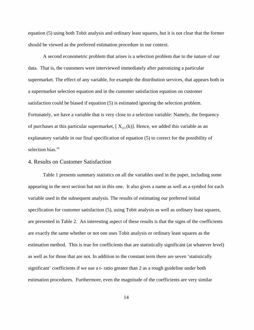
equation (5) using both Tobit analysis and ordinary least squares, but it is not clear that the former

should be viewed as the preferred estimation procedure in our context.

A second econometric problem that arises is a selection problem due to the nature of our

data. That is, the customers were interviewed immediately after patronizing a particular

supermarket. The effect of any variable, for example the distribution services, that appears both in

a supermarket selection equation and in the customer satisfaction equation on customer

satisfaction could be biased if equation (5) is estimated ignoring the selection problem.

Fortunately, we have a variable that is very close to a selection variable: Namely, the frequency

of purchases at this particular supermarket, [ Xi13 (k)]. Hence, we added this variable as an

explanatory variable in our final specification of equation (5) to correct for the possibility of

selection bias.16

4. Results on Customer Satisfaction

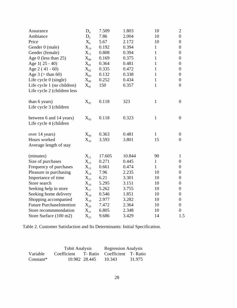
Table 1 presents summary statistics on all the variables used in the paper, including some

appearing in the next section but not in this one. It also gives a name as well as a symbol for each

variable used in the subsequent analysis. The results of estimating our preferred initial

specification for customer satisfaction (5), using Tobit analysis as well as ordinary least squares,

are presented in Table 2. An interesting aspect of these results is that the signs of the coefficients

are exactly the same whether or not one uses Tobit analysis or ordinary least squares as the

estimation method. This is true for coefficients that are statistically significant (at whatever level)

as well as for those that are not. In addition to the constant term there are seven ‘statistically

significant’ coefficients if we use a t- ratio greater than 2 as a rough guideline under both

estimation procedures. Furthermore, even the magnitude of the coefficients are very similar

15

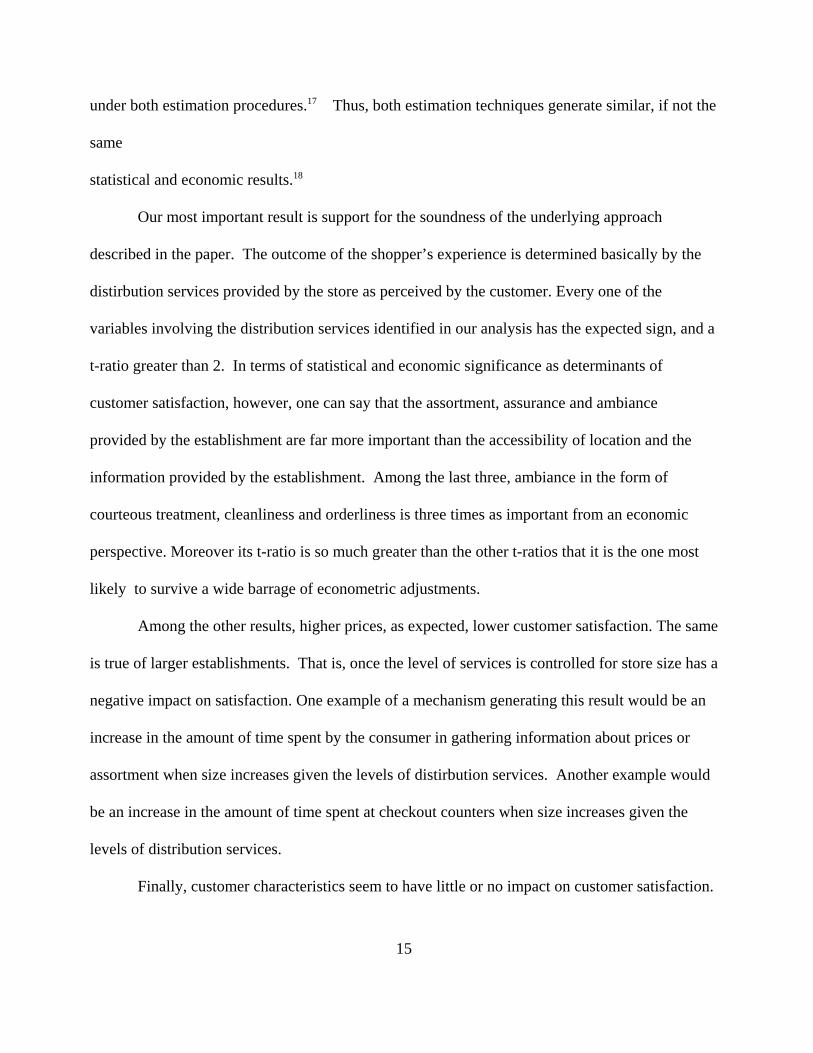
under both estimation procedures.17 Thus, both estimation techniques generate similar, if not the

same

statistical and economic results.18

Our most important result is support for the soundness of the underlying approach

described in the paper. The outcome of the shopper’s experience is determined basically by the

distirbution services provided by the store as perceived by the customer. Every one of the

variables involving the distribution services identified in our analysis has the expected sign, and a

t-ratio greater than 2. In terms of statistical and economic significance as determinants of

customer satisfaction, however, one can say that the assortment, assurance and ambiance

provided by the establishment are far more important than the accessibility of location and the

information provided by the establishment. Among the last three, ambiance in the form of

courteous treatment, cleanliness and orderliness is three times as important from an economic

perspective. Moreover its t-ratio is so much greater than the other t-ratios that it is the one most

likely to survive a wide barrage of econometric adjustments.

Among the other results, higher prices, as expected, lower customer satisfaction. The same

is true of larger establishments. That is, once the level of services is controlled for store size has a

negative impact on satisfaction. One example of a mechanism generating this result would be an

increase in the amount of time spent by the consumer in gathering information about prices or

assortment when size increases given the levels of distirbution services. Another example would

be an increase in the amount of time spent at checkout counters when size increases given the

levels of distribution services.

Finally, customer characteristics seem to have little or no impact on customer satisfaction.

16

This is true of general demographic characteristics, general attitudes toward purchase activities

and attitudes toward specific features of the establishment. Similarly, objective characteristics of

the purchase activity, for example the average size of the basket purchased by the customer, do

not matter in explaining customer satisfaction. Incidentally, firm dummies were included in the

Tobit analysis and in the OLS regression. None of the firm dummies were statistically significant

at the 1% level.

With respect to supermarkets the brand, captured by the firm dummies, adds little

differentiation given the levels of distribution services provided. Consumers base their evaluation

of satisfaction with the store mainly on the functional elements embedded in the services. Since

this shopping experience is characterized by routine, the every-day services performance

dominates the consumer’s evaluation. Halo attributes such as brand play a minor, if any, role in

the formation of satisfaction, especially in our case of transaction specific customer satisfaction.

Since our samples are generated by interviewing customers exiting a particular

establishment, as indicated before, one can argue that our coefficient estimates suffer from a

selection bias of the following nature. They reflect not only the impact of a variable on customer

satisfaction but also the impact of the same variable in attracting these customers to the store. In

order to control for this bias, we included as an explanatory variable a dummy, X13, that takes on

the value of unity when a customer frequents the store 4 or more times within a month and zero

otherwise. The results are presented in Table 3. They are exactly the same as we found in Table

2. Indeed, in the immense majority of cases the magnitudes of the coefficient estimates in Table 2

differ from the corresponding ones in Table 3 only after the second decimal place! The

coefficient of the new variable is positive, as expected, but it is not statistically significant at any

17

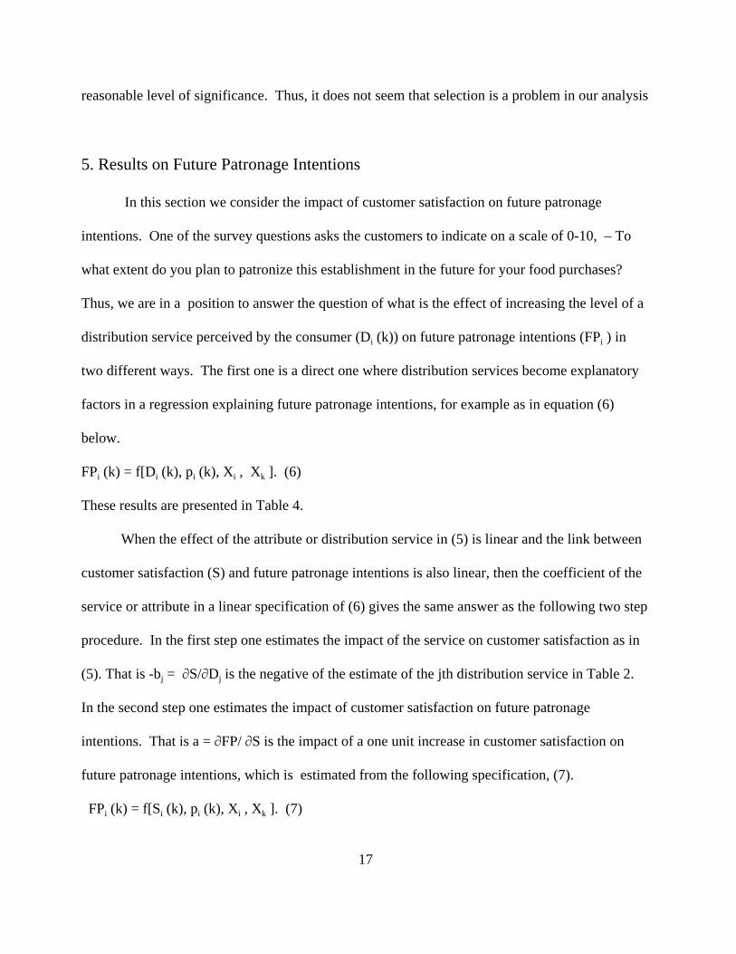
reasonable level of significance. Thus, it does not seem that selection is a problem in our analysis

5. Results on Future Patronage Intentions

In this section we consider the impact of customer satisfaction on future patronage

intentions. One of the survey questions asks the customers to indicate on a scale of 0-10, – To

what extent do you plan to patronize this establishment in the future for your food purchases?

Thus, we are in a position to answer the question of what is the effect of increasing the level of a

distribution service perceived by the consumer (Di (k)) on future patronage intentions (FPi ) in

two different ways. The first one is a direct one where distribution services become explanatory

factors in a regression explaining future patronage intentions, for example as in equation (6)

below.

FPi (k) = f[Di (k), pi (k), Xi , Xk ]. (6)

These results are presented in Table 4.

When the effect of the attribute or distribution service in (5) is linear and the link between

customer satisfaction (S) and future patronage intentions is also linear, then the coefficient of the

service or attribute in a linear specification of (6) gives the same answer as the following two step

procedure. In the first step one estimates the impact of the service on customer satisfaction as in

(5). That is -bj = MS/MDj is the negative of the estimate of the jth distribution service in Table 2.

In the second step one estimates the impact of customer satisfaction on future patronage

intentions. That is a = MFP/ MS is the impact of a one unit increase in customer satisfaction on

future patronage intentions, which is estimated from the following specification, (7).

FPi (k) = f[Si (k), pi (k), Xi , Xk ]. (7)

18

These results are presented in Table 5.

That the two methods will not give the same results is easy to see in our case. Not all

distribution services are statistically significant in Table 4. In particular, information is clearly not

and assurance of product delivery is not if we use a t-ratio of 2 as a strict guideline. Yet all

distribution services were ‘statistically significant’ in Table 2 and customer satisfaction (S) is

‘statistically significant ’ in Table 5. Hence, the two step procedure is valid for all five of them.

Given that the results differ, the two step procedure is presumed to be the appropriate one.

Because it is more general, for example it does not require linearity.19 In any event the literature

on customer satisfaction, while stressing the service/satisfaction/economic performance chain, has

not addressed the possibility of this difference in results from the two approaches.

Incidentally, three other strong results emerge from Tables 4 and 5, using a t-ratio of 2

with both estimation methods as a guide for reliable and robust results. The higher the frequency

of purchases, X 13 , the higher the score on the future patronage intentions variable with both

methods. Similarly, the more important is the time spent on this activity the lower is the score on

future patronage intentions of the consumer. Finally, the firm dummy variables are significantly

different from zero, indicating that intentions of future patronage are affected by different levels

of firm loyalty.20

To conclude the discussion we note briefly the economic and managerial implications of

our results. In order to evaluate the effect of a service on economic performance through the

service/satisfaction/intentions chain, the manager of a store needs to know the answer to two

questions First, – What is the impact on customer satisfaction of increasing the level of a

distribution service per unit cost? Namely,

19

MS/MDj / cj = -bj / cj . (8)

The piece of information in the numerator is the result of the statistical anlysis in the previous

section. The piece of information in the denominator in general should be available to the store

manager from knowledge and data on the operations of the store.21

Second, – What is the impact of increasing customer satisfaction by one unit on future

patronage intentions in terms of economic performance variables? Namely,

[MR/MFP][MFP/MS] = [MR/MFP] [a]. (9)

One piece of information comes from the statistical analysis in this section (a). Just as before the

first piece of information should be available to the store manager from knowledge and data on

the operations of the store. It is the expected amount of revenues generated by a unit increase in

future patronage intentions. Since a unit increase in FP is a movement of one unit in a scale of 0-

10, we can interpret it as an increase of .10 in the probability of a visit . Thus, .10 times the

average expenditures on a visit gives an estimate of [MR/MFP].

To illustrate with an example22: the expected revenues from increasing future purchase

intentions per customer by a unit [MR/MFP] are .10 times average yearly expenditures of $500. per

customer at the supermarket (= $50.); a one unit increase in customer satisfaction, however,

generates only a 0.463 increase in future purchase intentions [MFP/MS = a] and, thus, the $50.

increase becomes $23.15. Furthermore, a one unit increase in ambiance generates a 0.385 ( - bj )

increase in customer satisfaction. Hence, a one unit increase in ambiance generates an $8.91

(.385* 23.15) increase in revenues per customer. For a supermarket that has 100 customers, this

implies that it should undertake the costs of increasing ambiance by one unit as long as the costs

of doing so (cj ) are less than $891 per unit per year.23

20

6. Concluding Remarks

Our main contributions in this paper are the following. First, we integrate the literature on

the role of the consumer in retailing with the literature on customer satisfaction. We do so by

drawing the implications of viewing distribution services as outputs of retail firms and as fixed

inputs into the household production functions of consumers. The resulting conceptualization

provides a solid foundation for the analysis of customer satisfaction in retailing at the transaction

level. Second, we have implemented this framework empirically using a unique data set that

identifies distribution services explicitly. The results are sensible, robust and important.

Substantively these results imply that distribution services are the main mechanism through which

retailers can influence customer satisfaction with transactions at the supermarket level. Third, the

effects of distributions services on future purchase intentions are very different empirically when

estimated directly than when estimated as part of an attribute/satisfaction/future intentions chain.

All research has limitations and often these limitations are useful as guides to areas of

further research. Ours is no exception. First, operational implementation of our approach requires

supermarket managers to estimate the costs of increasing effort in the provision of distribution

services as well as estimating the expected benefits of an increase in future patronage intentions.

We used illustrative numbers here, but there are clear practical benefits to future research that

generates reliable estimates of these cosst and benefits . Second, our analysis focuses on

transaction specific customer satisfaction but extending the analysis to cumulative customer

satisfaction is an attractive area for future academic research. Finally, in our data we have

measured distribution services explicitly and this is an asset not a limitation. Nonetheless,

Barber and Tietje (2004) have shown how to measure them implicitly, i.e., extracting them from

21

the service attributes associated with store surveys using principal components. Therefore, a

comparison of the two approaches with respect to their effect on customer satisfacion and on

future purchase intentions would also be an interesting area for future research.

Notes

1. For a discussion of how distribution services affect retail equilibrium configurations see, for

example, Betancourt (2004, Chapter 2, Sections 4 and 5).

2. The primitives from which this cost function follows can be found in Betancourt (2004, Ch. 4).

22

3. The basis for this demand function can be found, for example, in Betancourt and Gautschi

(1990).

4. For instance, the fourth case is not economically interesting (at least in the short-run) because it

requires a dissatisfied customer, Dd > Ds ,and a retailer that can’t benefit from improving

satisfaction because she is operating at full capacity (Qd = Qs ).

5. A related consideration is whether the focus of the analysis is customer satisfaction with

specific transactions or cumulative customer satisfaction. Given the cross-section nature of our

data, we focus on the former rather than the latter.

6. For an example of a recent study eliciting estimates of consumer’s willingness to pay see

Chatterjee, Wang and Venkatesh (2005).

7. Every study of customer satisfaction that measures attributes on the basis of surveys makes this

assumption implicitly, if their concept is to be related to the original idea of quality relative to

expectations about quality. This is true of earlier constructs, for example Servqual, or of their

modern replacements ( customer service, quality and value) as used in, for example, Gomez,

Mclaughlin and Wittink (2003). One advantage of making the assumption explicit is to provide

guidance on how to relax it in the future; the other advantage is in connecting seemingly

unconnected strands of literatures.

8. There is a long tradition, with respect to supermarkets and other retail establishments where

surveys are undertaken, of asking a number of questions about services provided. These questions

can be mapped into the five distribution services stressed here. For instance, Barber and Tietje

(2004) look at 20 survey questions, reduce them to 14 in terms of relevance, and collapse these

remaining 14 into six categories through principal component analysis: the five distribution services

23

stressed here and one category that refers to price. What is unique about the Pamplona data is the

asking of direct questions in these surveys about four of the aggregate categories stressed here.

9. A supermarket in Pamplona is defined as a self-service establishment, usually between 250 and

2500 squared meters of surface area, with an assortment predominantly oriented toward food

products.

10. Of the 18 establishments qualifying as supermarkets in the Pamplona area 14 belong to 5 chains

(including one discount chain) and 4 are independent establishments. 3 of the 4 independent

establishments were selected together with a large and a small establishment from each of four

chains, including the discount chain.

11. Incidentally for one particular week, and evenly distributed through the daily opening hours,

consumers were selected to fill the survey upon exiting the supermarket.

12. For a more detailed description of these and subsequent variables see the data Appendix.

13. It turns out there are no observations for this variable that take on the value of zero ( and only

one that takes on the value of 1), but there are 161 that take on the value of 10.

14. For instance, see the discussion of censoring in Maddala (1983, Chapter 1).

15. For example, see Greene (2003, Chapter 22). Incidentally, other estimation issues in the context

of qualitative dependent variables lead Cortiñas (2004) to the use of neural networks as an

estimation technique.

16. One could argue that this induces a simultaneity problem if customer satisfaction is a

determinant of frequency of purchases. This argument is considerably weaker when one realizes that

the simultaneity problem is far more likely to exist with respect to cumulative customer satisfaction

than with respect to transaction specific customer satisfaction. The latter is what we are measuring

24

in our data.

17. For instance, except for the constant term, all the coefficients of ordinary least squares that have

a t-ratio greater than 2 are within one and a half standard deviation of the value of the corresponding

coefficient under Tobit analysis.

18. Incidentally, the R2 for the OLS procedure is .497, and the adjusted one is .481.

19. By the way, the unadjusted R2 in Table 4 is .305 whereas in Table 5 is .300. The adjusted ones

are .282 and .280, respectively.

20. None of these three types of variables mattered as determinants of customer satisfaction. For

completeness we also considered the variables that represented attitudes toward purchasing at this

establishment [X17 , X18, X19 ] in this estimation. When we included these variables the results with

respect to signs and statistical significance were the same as those discussed in the text.

21. In our case, since the benefits from increasing ambiance by one unit are almost three times

larger in magnitude (0.434/0.153) than the next best alternative (assortment), unit costs would have

to be almost three times as large to compensate for the advantage on the benefit side.

22. We use the results from the OLS regressions in this illustration.

23. Judging from the questions the costs of producing an additional unit of ambiance entail the

costs of training employees to be courteous and/or to provide cleanliness and orderliness in the store.

References

Anderson, E. and M. Sullivan (1993). “ The Antecedents and Consequences of Customer

Satisfaction for Firms,” Marketing Science 12 (Spring), 125- 43.

Anderson, E., C. Fornell and D. Lehman (1994). “Customer Satisfaction, Market Share

25

and Profitability,” Journal of Marketing 58 (July), 53- 66.

Anderson, E., C. Fornell and S. Mazvancheryl (2004). “ Customer Satisfaction and

Shareholder Value,” Journal of Marketing 68 (October), 172- 85.

Anderson, E. and V.Mittal (2000). “Strengthening the Satisfaction Profit Chain,” Journal of Service

Research 3 (2), 107-120.

Barber, C. and B. Tietje (2004). “A Distribution Services Approach for Developing Effective

Competitive Strategies Against ‘Big Box’ Retailers,” Journal of Retailing and Consumer

Services 11, 98-107.

Berne, C., J. M. Mugica and M.J. Yague (1999). “ Una Evaluacion de los Modelos de

Regresion Switching para la Medicion de la Productividad en el Comercio

Minorista,” Economia Industrial (326), 159- 72.

Betancourt, R. (2004). The Economics of Retailing and Distribution. London: Edward

Elgar Publishing, Ltd.

Betancourt, R. and D. Gautschi (1988). “ The Economics of Retail Firms,” Managerial

and Decision Economics 9, 133- 44.

______ (1990). “ Demand Complementarities, Household Production and Retail

Assortments,” Marketing Science 9, 146-61.

Bucklin, L. (1973). Productivity in Marketing. Chicago, Ill: American Marketing Association.

Chatterjee,R. T. Wang and R.Ventakesh (2005). “ Reservation Price as a Range: An Incentive

Compatible Measurement Approach,” paper presented at Informs Marketing Science

Conference in Atlanta.

CortiÁas, M. (2004). La Aplicacion de la Tecnica de Redes Neuronales Artificiales en la

26

Gestion del Comercio Minorista. Ph. D. Dissertation, Pamplona: Universidad

Publica de Navarra.

Greene, W. (2003). Econometric Analysis. New Jersey: Prentice Hall Co.

Gomez, M., E. McLaughlin and D. Wittink (2003). “ Do Changes in Customer

Satisfaction Lead to Changes in Sales Performance in Food Retailing,” New

Haven: Yale School of Management. Working Paper # 14.

Kamakura, W., V. Mittal, F. De Rosa and J.Mazzon (2002). “Assessing the Service-Profit Chain,”

Marketing Science 21 (Summer), 294-317.

Maddala, G.S. (1983). Limited- Dependent and Qualitative Variables in Econometrics.

London: Cambridge University Press.

Malthouse, E., J.Oakley, B. Calder and D. Iacobucci (2004).“Customer Satisfaction Across

Organizational Units,” Journal of Service Research 6 (February), 231-242.

Ofer, G. (1973). “ Returns to Scale in the Retail Trade,” Review of Income and Wealth 19, 363-84.

Oi, W. (1992). “Productivity in the Distributive Trades: The Shopper and the Economics of Massed

Reserves,” in Z. Griliches (ed.) Output Measurement in the Service Sector. Chicago:

University of Chicago Press.

Rust, R. and A. Zahoric (1993). “Customer Satisfaction, Customer Retention and Market

Share,” Journal of Retailing 69 (Summer), 193- 215.

Shaw, S., D. Nisbet and J. Dawson (1989). “ Economies of Scale in UK Supermarkets:

Some Preliminary Findings,” International Journal of Retailing 4, 12-26.

27

Table 1. Descriptive Statistics

Variable Name Symbol Mean Standard dev. Maximun MinimunSatisfaction S 7.823 1.665 10 1Location D1 7.857 2.456 10 0Information D2 7.343 2.254 10 0Assortment D3 7.314 2.321 10 0

28

Assurance D4 7.509 1.803 10 2Ambiance D5 7.86 2.004 10 0Price X6 5.67 2.172 10 0Gender 0 (male) X70 0.192 0.394 1 0Gender (female) X71 0.808 0.394 1 0Age 0 (less than 25) X80 0.169 0.375 1 0Age 1( 25 - 40) X81 0.364 0.481 1 0Age 2 ( 41 - 60) X82 0.335 0.472 1 0Age 3 (> than 60) X83 0.132 0.338 1 0Life cycle 0 (single) X90 0.252 0.434 1 0Life cycle 1 (no children) X91 150 0.357 1 0Life cycle 2 (children less

than 6 years) X92 0.118 323 1 0Life cycle 3 (children

between 6 and 14 years) X93 0.118 0.323 1 0Life cycle 4 (children

over 14 years) X94 0.363 0.481 1 0Hours worked X10 3.593 3.801 15 0Average length of stay

(minutes) X11 17.605 10.844 90 1Size of purchases X12 0.271 0.445 1 0Frequency of purchases X13 0.661 0.474 1 0Pleasure in purchasing X14 7.96 2.235 10 0Importance of time X15 6.21 3.301 10 0Store search X16 5.295 3.151 10 0Seeking help in store X17 5.262 3.755 10 0Seeking home delivery X18 0.546 1.851 10 0Shopping accompanied X19 2.977 3.282 10 0Future PurchaseIntention X20 7.472 2.364 10 0Store recommmendation X21 6.805 2.348 10 0Store Surface (100 m2) X22 9.686 3.429 14 1.5

Table 2. Customer Satisfaction and Its Determinants: Initial Specification.

Tobit Analysis Regression AnalysisVariable Coefficient T- Ratio Coefficient T- RatioConstant* 10.982 28.445 10.343 31.975

29

[10 - D1 ]* -0.05 -2.379 -0.047 -2.594[10 - D2 ]* -0.061 -2.33 -0.045 -2.01[10 - D3 ]* -0.152 -5.57 -0.13 -5.645[10 - D4 ]* -0.147 -4.216 -0.118 -3.971[10 - D5 ]* -0.439 -13.025 -0.388 -13.469X6* -0.067 -2.483 -0.051 -2.228X22* -0.039 -2.122 -0.036 -2.269X7 0.067 0.505 0.013 0.111X81 0.218 1.275 0.156 1.069X82 0.126 0.695 0.109 0.706X83 0.066 0.31 0.073 0.412X91 -0.102 -0.616 -0.103 -0.731X92 -0.247 -1.152 -0.193 -1.058X93 -0.141 -0.726 -0.074 -0.447X94 0.108 0.657 0.095 0.687X10 -0.023 -1.508 -0.018 -1.388X11 0,005 1.117 0.005 1.149X12 -0.151 -1.308 -0.14 -1.426X14 -0.012 -0.517 -0.013 -0.669X15 -0.02 -1.267 -0.015 -1.095X16 -0.019 -1.227 -0.008 -0.594F1 -0.404 -1.913 -0.321 -1.807F2 0.081 0.377 0.128 0.705F3 0.029 0.125 0.037 0.191F4 0.024 0.102 -0.007 -0.037F5 -0.394 -1.705 -0.29 -1.488F6 0.188 0.808 0.139 0.717

* t-ratio greater than 2 with both estimation methods

Table 3. Customer Satisfaction and Its Determinants: Selection Correction.

Tobit Analysis Regression AnalysisVariable Coefficient T- Ratio Coefficient T- RatioConstant* 10.897 27.,724 10.269 31.154[10 - D1 ]* -0.045 -2.103 -0.042 -2.302

30

[10 - D2 ]* -0.061 -2.347 -0.045 -2.025[10 - D3 ]* -0.154 -5.639 -0.132 -5.716[10 - D4 ]* -0.146 -4.193 -0.117 -3.947[10 - D5 ]* -0.435 -12.846 -0.385 -13.273X6* -0.067 -2.49 -0.051 -2.245X22* -0.039 -2.166 -0.036 -2.31X7 0.061 0.467 0.007 0.066X81 0.211 1.237 0.151 1.034X82 0.12 0.662 0.105 0.679X83 0.051 0.243 0.062 0.349X91 -0.106 -0.638 -0.107 -0.757X92 -0.249 -1.165 -0.196 -1.075X93 -0.15 -0.77 -0.082 -0.495X94 0.096 0.584 0.083 0.6X10 -0.022 -1.425 -0.017 -1.3X11 0.005 1.1 0.005 1.132X12 -0.129 -1.099 -0.12 -1.205X14 -0.01 -0.448 -0.011 -0.597X15 -0.02 -1.279 -0.015 -1.098X16 -0.019 -1.219 -0.008 -0.59X13 0.12 1.101 0.108 1.16F1 -0.407 -1.929 -0.325 -1.829F2 0.08 0.371 0.126 0.694F3 0.02 0.085 0.027 0.14F4 0.017 0.072 -0.015 -0.075F5 -0.405 -1.753 -0.299 -1.533F6 0.181 0.779 0.133 0.687

* t-ratio greater than 2 with both estimation methods

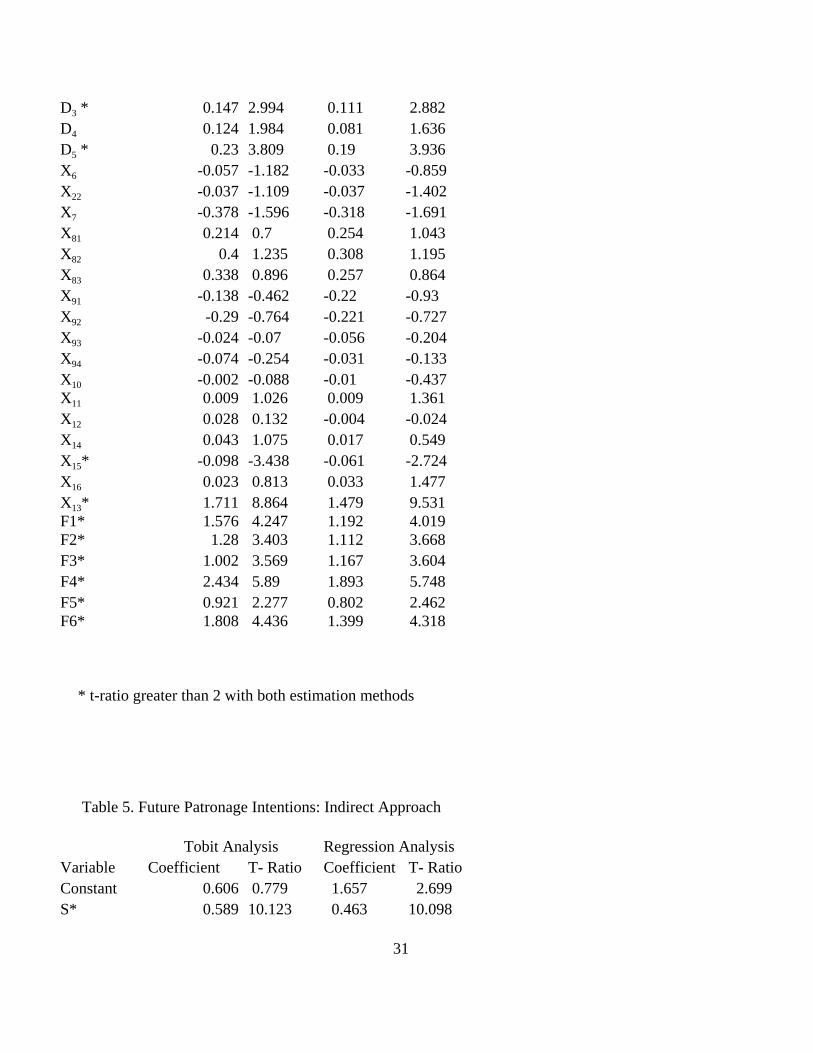
Table 4. Future Patronage Intentions: Direct Approach.

Tobit Analysis Regression AnalysisVariable Coefficient T- Ratio Cofficient T- RatioConstant 0.361 0.457 1.434 2.294D1 * 0.193 5.028 0.168 5.467D2 0.047 0.993 0.031 0.842

31

D3 * 0.147 2.994 0.111 2.882D4 0.124 1.984 0.081 1.636D5 * 0.23 3.809 0.19 3.936X6 -0.057 -1.182 -0.033 -0.859X22 -0.037 -1.109 -0.037 -1.402X7 -0.378 -1.596 -0.318 -1.691X81 0.214 0.7 0.254 1.043X82 0.4 1.235 0.308 1.195X83 0.338 0.896 0.257 0.864X91 -0.138 -0.462 -0.22 -0.93X92 -0.29 -0.764 -0.221 -0.727X93 -0.024 -0.07 -0.056 -0.204X94 -0.074 -0.254 -0.031 -0.133X10 -0.002 -0.088 -0.01 -0.437X11 0.009 1.026 0.009 1.361X12 0.028 0.132 -0.004 -0.024X14 0.043 1.075 0.017 0.549X15* -0.098 -3.438 -0.061 -2.724X16 0.023 0.813 0.033 1.477X13* 1.711 8.864 1.479 9.531F1* 1.576 4.247 1.192 4.019F2* 1.28 3.403 1.112 3.668F3* 1.002 3.569 1.167 3.604F4* 2.434 5.89 1.893 5.748F5* 0.921 2.277 0.802 2.462F6* 1.808 4.436 1.399 4.318

* t-ratio greater than 2 with both estimation methods

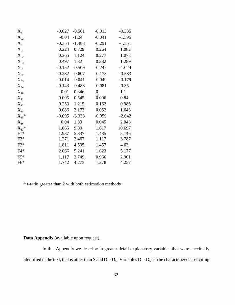
Table 5. Future Patronage Intentions: Indirect Approach

Tobit Analysis Regression AnalysisVariable Coefficient T- Ratio Coefficient T- RatioConstant 0.606 0.779 1.657 2.699S* 0.589 10.123 0.463 10.098

32

X6 -0.027 -0.561 -0.013 -0.335X22 -0.04 -1.24 -0.041 -1.595X7 -0.354 -1.488 -0.291 -1.551X81 0.224 0.729 0.264 1.082X82 0.365 1.124 0.277 1.078X83 0.497 1.32 0.382 1.289X91 -0.152 -0.509 -0.242 -1.024X92 -0.232 -0.607 -0.178 -0.583X93 -0.014 -0.041 -0.049 -0.179X94 -0.143 -0.488 -0.081 -0.35X10 0.01 0.346 0 1.1X11 0.005 0.545 0.006 0.84X12 0.253 1.215 0.162 0.985X14 0.086 2.173 0.052 1.643X15* -0.095 -3.333 -0.059 -2.642X16 0.04 1.39 0.045 2.048X13* 1.865 9.89 1.617 10.697F1* 1.937 5.337 1.485 5.146F2* 1.271 3.467 1.117 3.787F3* 1.811 4.595 1.457 4.63F4* 2.066 5.241 1.623 5.177F5* 1.117 2.749 0.966 2.961F6* 1.742 4.273 1.378 4.257

* t-ratio greater than 2 with both estimation methods

Data Appendix (available upon request).

In this Appendix we describe in greater detail explanatory variables that were succinctly

identified in the text, that is other than S and D1 - D5. Variables D1 - D5 can be characterized as eliciting

33

consumer’s perceptions of how well the supermarket was providing a distribution service or a selected

aspect or dimension of a distribution service. The information in Table 1 shows substantial variations

in these perceptions across consumers despite the fact that all 11 supermarkets considered belonged to

the same type or format. In addition to these variables, essential for our purposes, the survey gathered

information on general characteristics of consumers and specific characteristics of their buying habits,

including attitudes toward purchasing.

Variables X7 - X10 measure general characteristics of consumers. X7 identifies gender (one if

the consumer is female). Age, X8 , is captured through dummy variables where the omitted category

is that the consumer is less than 25. (X81) is one if the consumer is between 25 and 40 years of age. (X82

) is one if she is between 41 and 60. Finally (X83 ) is one if the consumer is greater than 60 years old.

Position in the life cycle, X9 , was captured in terms of dummy variables where the omitted category

was single without children. (X91 ) is one if the consumer is part of a couple without children. (X92 ) is

one if the consumer has children less than 6 years old. (X93 ) is one if the consumer has children

between 6 and 14 years. (X94 ) is one if the consumer has children over 14 years. The last of these

variables, X10 , measures the number of hours worked outside the home during the day by the consumer.

Among the specific characteristics of their buying habits consumers were asked about the

following: average length of their stay in the establishment in minutes, X11 , average size of their basket

in pesetas, X12 , and frequency of patronage of the establishment within the month, X13 . X12 was

originally measured as a categorical variable (1 – less than 2000 pesetas (12 euros); 2 – 2000 < x <

5000; 3 – 5000 < x < 10,000; and 4 greater than 10,000) and we redefined it as a dummy taking on the

value of unity for large purchases (categories 3 and 4) and zero otherwise. X13 was also redefined by

us as a dummy that took on the value of unity if the answer was more than 4 times a month and zero

34

otherwise.

With respect to their attitudes toward purchasing in supermarkets consumers were asked the

following: To what extent do you enjoy doing the purchasing of food products by yourself?, X14 ; To

what extent is it important for you to reduce the amount of time spent on this activity?, X15 ; To what

extent do you search for alternative establishments when doing this type of purchasing?, X16 . Finally,

consumers were also asked: Out of ten times that you buy fresh products at this establishment, how

many of them would you ask for employee help?, X17 ; Out of ten times that you patronize the

establishment, how many of them do you ask the establishment to deliver products to your home?, X18;

Out of ten times that you patronize the establishment, how many of them do you do so in the company

of some one?, X19 .

A number of questions were asked to capture a consumer’s attitude toward the establishment.

One of them,X20 , asks – To what extent do you plan to patronize this establishment in the future for

your food purchases? Another one, X21 , asks – To what extent would you recommend this

establishment to other persons? In addition information was collected from the managers of the 11

establishments on characteristics of the establishment such as surface area (X22 ), number of registers,

number of employees and number of hours the establishment was open.