The Cross Section of Bank Value∗

Mark Egan

University of Minnesota

Stefan Lewellen

London Business School

Adi Sunderam

Harvard Business School

November 10, 2016

Abstract

We study the determinants of value creation within U.S. commercial banks. We

begin by constructing two new measures of bank productivity: one focused on deposit-

taking productivity and one focused on asset productivity. We then use these measures

to evaluate the cross-section of bank value. Both productivity measures are strongly

value-relevant, with variation in banks' deposit productivity responsible for the majority

of variation in bank value. We also �nd evidence consistent with synergies between

deposit-taking and lending activities: banks with high deposit productivity have high

asset productivity, a relationship driven by the tendency of deposit-productive banks to

hold illiquid loans. Our results suggest that both sides of the balance sheet contribute

meaningfully to bank value creation, with the liability side playing a primary role.

∗Email addresses: eganx076@umn.edu, slewellen@london.edu, asunderam@hbs.edu. We thank AnilKashyap, Henri Servaes, Vania Stavrakeva, Chad Syverson, Vikrant Vig, and seminar participants atCarnegie Mellon University and London Business School for helpful comments. Lewellen thanks the Re-search and Materials Development Fund at London Business School for generous �nancial support. Sunderamgratefully acknowledges funding from the Harvard Business School Division of Research.

1 Introduction

How do commercial banks create value? Forty years of theoretical work has identi�ed three

potential answers to this question. First, banks can create value by providing safe and liquid

liabilities to depositors (e.g., Gorton and Pennacchi, 1990; Dang, Gorton, and Holmstrom,

2015). Second, banks can create value through their ability to screen and monitor loans

(e.g., Diamond, 1984). Finally, synergies between deposit-taking and lending may create

value by allowing banks to make certain types of loans more easily than other intermediaries

(e.g., Diamond and Dybvig 1983; Kashyap, Rajan, and Stein, 2002). To date, the empir-

ical literature has documented evidence consistent with each channel: banks do appear to

produce safe assets, to make information-intensive loans involving screening and monitoring,

and to make loans that are synergistic with deposit-taking. However, little is known about

the value implications of these channels, either individually or collectively.

In this paper, we construct novel measures of productivity for both sides of a bank's

balance sheet and use these productivity measures to assess the key determinants of bank

value creation. We begin by constructing estimates of banks' productivity at raising deposits.

To do so, we estimate a demand system for bank deposits following Dick (2008) and Egan,

Hortaçsu, and Matvos (2016). Banks compete for deposits by setting interest rates in a

standard Bertrand-Nash di�erentiated products setting, which we estimate using a common

model of demand from the industrial organization literature (Berry, 1994; Berry, Levinsohn,

and Pakes, 1995). Our demand estimates provide insight into consumer preferences for

deposit rates and other banking services. We then use these demand estimates to quantify

deposit productivity at the bank-year level. Intuitively, a bank with a high degree of deposit

productivity is able to collect more deposits than a less-productive bank, holding �xed input

variables such as the o�ered deposit rate and the number of branches the bank operates.

We next turn to the asset side of banks' balance sheets. Using standard methods, we

�exibly estimate a bank's ability to produce interest and fee income as a function of its loan

and securities portfolios. As in the literature on estimating total factor productivity (see

Syverson, 2011), we use the residuals and bank �xed e�ects from the estimated production

function as our measure of asset productivity for individual banks. Intuitively, a bank with

higher asset productivity is able to generate higher levels of risk-adjusted revenue with the

same asset base as a less-productive bank. Hence, our estimation procedure allows us to

construct two complementary measures of bank productivity: a bank's skill at producing

deposits, and the same bank's skill at using these funds to generate revenue.

We use our productivity estimates to present four main results. First, our measures of

productivity are strongly value-relevant in the cross section of banks. High deposit produc-

1

tivity is associated with low interest expense (as a fraction of assets) for banks. Similarly,

high asset productivity is associated with high interest income, even after including a battery

of controls for bank risk taking. Most importantly, our measures of productivity are strongly

related to stock market-based measures of value like market-to-book ratios.

Our second main result is that cross-sectional variation in deposit productivity accounts

for the majority of cross-sectional variation in bank value. Using the structure provided by

our empirical framework, we are able to decompose bank value into the part attributable to

deposit productivity and the part attributable to asset productivity. We �nd that variation

in deposit productivity accounts for about twice as much variation in bank value as variation

in asset productivity. We also �nd similar results in reduced-form empirical tests that do

not rely on the structure of our framework. In particular, the relationship between deposit

productivity and bank market-to-book ratios is about twice as strong as the relationship

between asset productivity and market-to-book. A one-standard deviation increase in deposit

productivity is associated with an increase in market-to-book ratios of 0.2 to 0.5 points,

while a one-standard deviation increase in asset productivity is associated with an increase

in market-to-book of 0.1 to 0.2 points. Collectively, these �ndings suggest that liability-

driven theories of bank value creation explain more variation in the cross section of banks

than asset-driven theories.

In our third set of results, we explore the drivers of variation in our productivity measures

by examining cross-sectional variation in bank balance sheet composition. Consistent with

intuition, we �nd that high deposit productivity is associated with balance sheet liabilities

that are tilted towards deposits. A one-standard deviation increase in deposit productivity

is associated with a 1.8 standard deviation increase in the fraction of bank liabilities that

is made up of deposits. Interestingly, we �nd strong e�ects for both transaction and non-

transaction deposits (e.g., savings and time deposits), with the strongest e�ect coming from

savings deposits. Thus, while our estimates suggest that liabilities are an important source

of bank value, the liabilities that are most strongly associated with deposit productivity are

not necessarily those that provide the most transaction and liquidity services. In addition,

we �nd that the impact of deposit productivity on overall bank leverage is relatively small

in the cross section. Thus, banks that are particularly good at raising deposits are not

signi�cantly more levered than those that are not. Instead, they seem to be substituting

non-deposit debt for deposits.

We also �nd that banks with high asset productivity tilt their balance sheet towards

holding more illiquid assets. In particular, asset-productive banks hold more loans and fewer

securities. A one-standard deviation increase in asset productivity is associated with an

increase in the fraction of assets comprised of loans by 0.7 standard deviations (or approx-

2

imately 9 percentage points). Furthermore, when we look within banks' loan portfolios, we

�nd that more productive banks tend to hold higher levels of real estate and commercial

and industrial (C&I) loans, which are arguably more information-intensive than other types

of loans. Hence, our results are consistent with the idea that screening and monitoring of

information-intensive loans is an important source of bank value, though it accounts for less

variation in bank value than deposit productivity.

Finally, we utilize our productivity measures to assess the degree of synergies between

banks' deposit-taking and lending activities. Intuitively, a bank that is good at producing

deposits may be able to o�er more loans or di�erent types of loans than a bank that is less

productive at raising deposits. By assessing the relationships between our two productivity

measures, and by examining the relationship between each productivity measure and banks'

balance sheet composition, we are able to uncover di�erent types of synergies in a manner

distinct from the existing literature.

We �nd evidence of signi�cant synergies between the asset and liability sides of bank bal-

ance sheets. Speci�cally, asset productivity is strongly correlated with deposit productivity.

We use balance sheet composition to explore the sources of these synergies. We �nd that

deposit-productive banks tend to o�er more loan commitments and lines of credit, while

holding less securities and cash. A one standard deviation in deposit productivity is associ-

ated with a 0.6 standard deviation increase in the fraction of bank assets comprised of loan

commitments and lines of credit. Consistent with Kashyap, Rajan, and Stein (2002) and the

empirical evidence in Gatev and Strahan (2006), this result suggests that deposit-productive

banks �nd it relatively easy to meet unpredictable liquidity needs associated with providing

commitments, likely because they tend to attract deposit in�ows at the times when lines of

credit are drawn down.

In addition, we �nd that banks with high deposit productivity tend to make more loans,

particularly C&I loans. A one-standard deviation increase in deposit productivity is as-

sociated with an increase in the fraction of assets made up of C&I loans by 0.7 standard

deviations (or approximately 5 percentage points). Since C&I loans are more illiquid than

mortgage loans, this suggests that the ability to raise deposits in a cost-e�ective manner

is important for banks that wish to make pro�table, illiquid loans. This is consistent with

Hanson, Shleifer, Stein, and Vishny (2016), who argue that the fact that deposits are stickier

than other types of short-term debt is a key source of value for banks because it allows them

to hold more illiquid assets than they otherwise could.

Our four main �ndings are robust to a battery of additional tests and empirical speci-

�cations. For example, we �nd similar results when we re-estimate deposit demand using

di�erent de�nitions of a deposit market and re-estimate our asset income production func-

3

tion using a host of additional controls for risk. We also address potential measurement error

issues with our productivity measures by using instrumental variables and constructing em-

pirical Bayes estimates.1 Finally, we show that our results are not driven by the �nancial

crisis and are not an artifact of extreme outliers in our data.

In summary, this paper represents the �rst attempt to empirically identify the primary

determinants of cross-sectional variation in bank value. We focus on three theoretically mo-

tivated drivers of bank value: safety and liquidity services produced by deposits, screening

and monitoring technologies for lending, and synergies between deposit-taking and lend-

ing. While we �nd that all three drivers play an important role, our results suggest that

cross-sectional variation in deposit productivity accounts for the majority of cross-sectional

variation in bank value. Consistent with the idea that bank liabilities are �special,� we �nd

that a bank's deposit productivity plays an extremely important role in determining its

funding structure, its size, and its ultimate value.

Our paper is related to several strands of the literature on banking. First, a large theo-

retical and empirical literature has argued that banks create value by producing safe, liquid

liabilities that are useful for transaction purposes.2 Our paper adds to this literature by

evaluating the e�ects of safe-liability creation on bank value. Consistent with this literature,

we �nd strong evidence that bank value is linked to a bank's ability to produce safe, liquid

deposits. However, while a bank's transaction deposit productivity is linked to its value, our

strongest results are for savings deposits, which, while safe, are not completely liquid. In

addition, we �nd no evidence that non-deposit debt creates value for banks.

Second, our paper is related to a long literature on bank information production dating

back to Leland and Pyle (1977) and Diamond (1984).3 This literature has argued that part of

1Recent work in the education and labor literature has used empirical Bayes estimates to measure valueadded (e.g., Jacob and Lefgren, 2008; Kane and Staiger, 2008; and Chetty, Friedman, and Rockho�, 2014).

2For the theoretical literature, see, e.g., Gorton and Pennacchi, 1990; Pennacchi, 2012; Stein, 2012;Gennaoili, Shleifer, and Vishny, 2013; DeAngelo and Stulz, 2015; Dang, Gorton, and Holmström, 2015;Dang, Gorton, Holmström, and Ordoñez, 2016; Moreira and Savov, 2016. The empirical literature in thisarea, e.g., Krishnamurthy and Vissing-Jorgensen, 2012; Gorton, Lewellen, and Metrick, 2012; Greenwood,Hanson, and Stein, 2016; Krishnamurthy and Vissing-Jorgensen, 2015; Sunderam, 2015; and Nagel, 2016,has largely focused on understanding whether bank liabilities are special by examining the behavior ofequilibrium prices and quantities.

3Other asset-driven theories of bank value creation include Ramakrishnan and Thakor (1984), Boyd andPrescott (1986), Allen (1990), Diamond (1991), Rajan (1992), Winton (1995), and Allen, Carletti, andMarquez (2013). Empirical literature on the subject includes Petersen and Rajan (1994), Berger and Udell(1995), Demsetz and Strahan (1997), Shockley and Thakor (1997), Acharya, Hassan, and Saunders (2006),and Su� (2007). A separate literature argued that banks historically possessed �charter value� due to entryrestrictions that allowed incumbents to extract monopoly rents. However, charter values in the U.S. havee�ectively disappeared as a result of the removal of entry restrictions in the 1980s and 1990s. See Keeley(1990) for a discussion of the decline in charter values and Jayaratne and Strahan (1996) for more informationon the removal of branching restrictions. There is also a literature on estimating bank production functions,primarily for the purpose of understanding whether there are economies of scale in banking (e.g., Berger

4

a bank's purpose is to perform delegated information production and portfolio management

(e.g. screening and monitoring) on behalf of its investors. Consistent with the broad themes

of this literature, we �nd evidence that a bank's asset productivity is strongly linked to its

value. However, we also �nd that di�erences in asset productivity across banks appear to

be signi�cantly less important in the cross-section relative to di�erences in banks' abilities

to produce deposits.

A third literature has argued that banks exist in part because of built-in synergies between

their deposit-taking and lending activities.4 Consistent with this literature, we �nd that

deposit-productive banks also tend to be asset-productive. In particular, we document two

types of synergies. First, we �nd a positive correlation between banks' deposit productivity

and the quantity of loan commitments and lines of credit on their balance sheets. Second,

we �nd that deposit-productive banks hold a higher quantity of illiquid loans. Hence, our

results are broadly consistent with the notion that both sides of the balance sheet contribute

signi�cantly to bank value.

Finally, our paper is related to the growing literature at the intersection of industrial

organization and �nance. Our paper relates to a recent set of papers that build on the

industrial organization literature to estimate demand for �nancial products.5 On the asset

side, we estimate a bank's asset production function and productivity using a �rst order

approximation, similar to the techniques Maksimovic and Phillips (2001) and Schoar (2002)

use to study non�nancial �rms. An advantage in our setting is that we correct for the

potential endogeneity of production inputs using cost shifters from the liability side of the

bank as instruments.

The remainder of this paper is organized as follows. Section 2 presents a simple framework

that highlights the economic linkages between deposit productivity, asset productivity, and

and Mester, 1997; Hughes and Mester, 1998; Stiroh, 2000; Berger and Mester, 2003; Rime and Stiroh,2003; Wang, 2003). We extend this literature by estimating a bank's liability productivity in addition tointroducing a new methodology to estimate bank asset productivity and studying the value implications ofboth measures.

4See, e.g., Diamond and Dybvig (1983), Calomiris and Kahn (1991), Berlin and Mester (1999), Diamondand Rajan (2000, 2001), Kashyap, Rajan, and Stein (2002), Gatev and Strahan (2006), and Hanson, Shleifer,Stein, and Vishny (2016). Mehran and Thakor (2011) argue that there are synergies between equity capitaland lending and provide evidence from the cross section of bank valuations. Berger and Bouwman (2009)construct a measure of bank liquidity creation and show that their measure is positively correlated with banks'market-to-book ratios. Bai, Krishnamurthy, and Weymuller (2016) also link a bank's �liquidity mismatch�� roughly, the di�erence in liquidity between the asset and liability sides of a bank's balance sheet � to thebank's stock returns. However, neither of these papers perform a comprehensive analysis of the determinantsof bank value. To our knowledge, our paper is the �rst in the literature to do so.

5Our deposit demand estimates relate most closely to Dick (2008) and Egan, Hortaçsu, and Matvos(2016). Similar tools have been employed to estimate demand for other �nancial products such as Hortaçsuand Syverson (2004) for index mutual funds, Koijen and Yogo (2015) for investment assets, Koijen and Yogo(2016) for life insurance, and Hastings, Hortaçsu and Syverson (2016) for privatized social security.

5

bank value. Section 3 describes our estimation procedure and provides more details on our

measures of bank productivity. Our main results are discussed in Section 4, which relates

our productivity measures to bank characteristics and measures of bank value. Section 5

presents robustness exercises, and Section 6 concludes.

2 Economic Framework

In this section, we present a simple economic framework that allows us to link deposit

productivity and asset productivity with bank value. Our framework contains two types

of agents: consumers and banks. We begin by describing consumer preferences for bank

deposits. We then turn to the problem of banks seeking to generate revenue from their

assets.

2.1 Consumers

There is a continuum of consumers, each of whom chooses to deposit their funds at one

bank or purchase an outside option. Consumer demand for deposit services is a function

of the deposit rate and quality of services provided by each bank j = 1, ..., J. A consumer

depositing funds at bank j earns the deposit rate ij, which yields utility αij.6The parameter

α > 0 measures the consumer's sensitivity to deposit rates. Depositors also derive utility

from banking services, given by βXj + δj + εij. This �service utility� depends on observable

bank characteristics Xj, such as the number of bank branches. In addition, it depends on

a bank-speci�c �xed e�ect, δj, which re�ects bank quality di�erences: all else equal, some

banks o�er better services than others. Finally, the term εij is a consumer-bank speci�c

utility shock. This utility shock captures preference heterogeneity across consumers. Some

consumers may inherently prefer Bank of America to Citibank (or vice versa). Thus, the

total indirect utility7 derived by a depositor i from bank j is given by:

uij = αij + βXj + δj + εij. (1)

The bank speci�c �xed e�ects, δj, denote a bank's deposit productivity. Conditional on the

o�ered deposit rate (ij) and other bank characteristics (Xj), banks with a higher deposit

productivity δj are able to attract more deposits.

6While our empirical analysis uses panel data, we suppress time subscripts here for simplicity.7Our utility formulation closely follows that of Egan, Hortaçsu and Matvos (2016) with one notable

exception. Previous research such as Egan, Hortaçsu and Matvos (2016) and Rose (2015) �nd that depositors(particularly uninsured depositors) may be sensitive to the �nancial stability of a bank. Here we treatconsumers' perceptions about the bank's solvency as part of the bank's deposit productivity.

6

Consumers select the bank that maximizes their utility. We follow the standard assump-

tion in the industrial organization literature (Berry, 1994; Berry, Levinsohn, and Pakes,

1995) and assume that the utility shock εij is independently and identically distributed

across banks and consumers and follows a Type 1 Extreme Value distribution. Given this

distributional assumption, the probability that a consumer selects bank j follows the multi-

nomial logit distribution. We also assume that consumers have access to an outside good,

which represents placing funds outside of the traditional depository banking sector. Without

loss of generality, we normalize the utility of the outside good to zero (u0 = 0). The market

share for bank j, denoted sj, is then

sj (ij, i−j) =exp(αij + βXj + δj)∑J

k=1 exp(αik + βXk + δk) + 1. (2)

The total market size for deposits is denoted M. Hence, the total deposits collected by bank

j is sjM.

2.2 Banks

We next turn to the problem of banks. Banks collect deposits and other capital and invest

them in a bank-speci�c technology. Banks have total assets equal to to the sum of the

deposit it collects, Msj, and its other capital, Kj:

Aj = Mtsj +Kj.

The bank's per-period pro�t function is given by

πj = φjAθj − ijMtsj − rjKj. (3)

The term φjAθj re�ects the investment income the bank generates from assets Aj. In other

words, φjAθj is the bank's asset production function. For ease of exposition, we assume

that the income generated from the the bank's investment is deterministic. This allows us

to abstract away from bank risk-taking, which we address in our empirical analysis. The

parameter θ re�ects returns to scale in production, and φj re�ects bank j's asset productivity.

Speci�cally, φj re�ects excess risk-adjusted revenue the bank can earn on its loans and

securities. These revenues may arise because the bank has a particularly good technology

for screening and monitoring borrowers, or because it is particularly good at �nding and

holding mispriced securities. The remaining terms in the pro�t function, ijMsj and rjKj,

re�ect the bank speci�c costs of raising deposits Msj and capital Kj.

7

Banks compete for deposits by playing a di�erentiated product Bertrand-Nash interest

rate setting game. The bank sets the deposit rate to maximize

maxiφjA

θj − ijMsj − rjKj.

The corresponding bank �rst order condition is given by8

φjθAθ−1j =

(1

α(1 − sj)+ ij

). (4)

The left-hand side term, φjθAθ−1j , re�ects the marginal return of an additional dollar of

assets. The right-hand side term, 1α(1−sj) + ij, re�ects the marginal cost of collecting an

additional dollar of deposits. All else equal, banks with better investment opportunities

(higher marginal returns) will �nd it optimal to o�er higher deposit rates.

2.3 Bank Value and Productivity

The primary objects of interest in our simple framework are deposit and asset productivity.

We examine how these di�erent measures of productivity create value for the bank. On

the liability side, the parameter δj can be interpreted as a bank's total factor productivity

for collecting deposits, or simply bank j′s deposit productivity. Holding the o�ered deposit

rate (ij) and other bank characteristics (Xj) �xed, banks with a higher δj are able to attract

more depositors. In other words, banks with higher deposit productivity can attract deposits

more cheaply. To illustrate, suppose that bank j wishes to collect D deposits. It then needs

to o�er a deposit rate i0 such that D = Msj(i0, i−j). Bank j

′s interest expenditure is then

given by

Di0 = M

(exp(αi0 + βXj + δ0j )∑J

k=1 exp(αik + βXk + δk) + 1

)i0,

where δ0j re�ects bank j′s initial deposit productivity. Now, suppose that bank j's deposit

productivity increases from δ0j to δ1j . Because of the increase in productivity, bank j can now

o�er a lower rate equal to i1 = i0− δ1j−δ0j

αand still raise the the same amount of deposits, D.9

Bank j′s total interest expense of collecting D deposits falls by D(δ1j−δ

0j

α

). All else equal,

an increase in a bank's deposit productivity leads to an increase in the bank's net income

8For simplicity, we assume a bank's only choice variable is the deposit rate. However, the model can beeasily generalized to include additional choice variables, such as capital and risk. Provided that the additionalbank choice variables and deposit rates are determined simultaneously, the bank's �rst order condition fordeposit rates will remain the same because of the envelope theorem.

9Note that as illustrated by Eq. (4), a bank would �nd it optimal to increase the amount of deposits itcollects in equilibrium after an increase in productivity.

8

and bank value.

On the asset side, the parameter φj re�ects a bank's asset total factor productivity or

simply a bank's asset productivity. Conditional on the bank's level of assets, a bank with

higher asset productivity generates more revenue from its set of assets Aj. To illustrate,

suppose a bank's asset productivity increases from φ0j to φ

1j . All else equal, the increase in

asset productivity results in an increase in net income of (φ1 − φ0)Aθj . Both increases in

deposit productivity and asset productivity translate directly into higher net income and

value.

3 Data and Estimation

3.1 Data

Our primary data source is the Federal Reserve FR Y-9C reports, which provide detailed

quarterly balance sheet and income statement data for all U.S. bank holding companies. We

supplement the Y-9C data with stock market data from CRSP and weekly branch-level data

on advertised deposit rates from RateWatch. We also obtain branch-level deposit quantities

from the annual FDIC Summary of Deposits �les.

Our sample is the universe of public bank holding companies. Our primary data set

consists of an unbalanced panel of 847 bank holding companies over the period 1994 through

2015.10 Observations are at the bank holding company by quarter level. Table 1 provides

summary statistics for the data set. On average, bank deposit interest expenditure is 2.19%

and is 1.74% when measured net of fees. As discussed below, we measure the quality of

services o�ered by a bank using the bank's non-interest expenditures, number of employees,

and number of branches. Our two primary measures of bank risk taking are its equity beta

and its standard deviation of return on assets. Following Baker and Wurgler (2015), we

calculate the equity beta for each bank in our sample using monthly returns over the past

twenty-four months. Similarly, we measure the standard deviation of return on assets using

quarterly returns over the past two years. We provide further details and the source of each

variable in the data appendix.

3.2 Bank Liabilities: Deposit Demand Estimation

We estimate the demand system described in Section 2.1 using our bank data set over the

period 1994 through 2015. We can write the logit demand system in Eq. (2) as the following

10On average, we observe 327 banks in a given time period (quarter) and 52 observations (quarterly) foreach bank.

9

regression speci�cation:

lnMtsjt − ln(Mts0t) = αijt + βXjt + δjt. (5)

Because we do not observe the characteristics of the outside good, s0, we include a time

�xed e�ect. This also allows us to estimate the key demand parameters without actually

specifying the outside good. Thus, we estimate the following speci�cation:

lnMtsjt = αijt + βXjt + µj + µt + ξjt. (6)

We estimate demand in two separate ways. First, in our baseline demand speci�cations,

we de�ne the market for deposits and compute the associated bank market shares at the

aggregate US by quarter level. We also estimate a second demand system where we de�ne

the market for deposits at the county by year level.11

A standard issue in demand estimation is the endogeneity of prices, or in this case,

deposit rates. The term ξjt in Eq. (6) represents an unobserved bank-time speci�c demand

shock. Alternatively, it could be viewed as the unobserved time varying component of bank

j's deposit service quality at time t. If banks observe ξjt prior to setting deposit rates, the

o�ered deposit rate will be correlated with the unobservable term ξjt. For example, suppose

bank j experiences a demand shock such that ξjt is positive. Bank j will then �nd it optimal

to o�er a lower deposit rate (e.g., Eq. 4). This will cause our estimate of α to be biased

downwards.

We employ an instrumental variables strategy to account for the endogeneity of deposit

rates. We have two sets of instruments. First, following Villas-Boas (2007) and Egan, Hor-

taçsu, and Matvos (2016), we construct instruments from the bank speci�c pass-through of

3-month LIBOR into deposit rates. As documented by Hannan and Berger (1991), Neumark

and Sharpe (1992), Driscoll and Judson (2013), and Drechsler, Savov, and Schnabl (2016),

deposit rates at di�erent banks respond di�erently to changes in short term interest rates.

Investment opportunities are a key reason for this variation. Banks with good investment

opportunities will not wish to lose deposit funding to competitors and thus will raise their

deposit rates more when short rates rise. Hence, variation in investment opportunities will

induce variation in deposit rates that is unrelated to the deposit demand conditions that

banks face. Thus, we can instrument for ijt, the deposit rate o�ered by bank j at time t,

with the �tted value of a bank-speci�c regression of ijt on 3-month LIBOR. The exclusion

restriction in this setting is that bank j's average degree of pass-through in the time series

11Deposit market share data at the branch level is only available at an annual frequency through theFDIC's Summary of Deposits. Hence, we estimate demand at the county level using annual data.

10

is orthogonal to the deposit demand it faces at time t.

Our second set of instruments are traditional Berry, Levinsohn, and Pakes (1995)-type

instruments. We instrument for deposit rates using the average product characteristics of a

bank's competitors. To help rule out potential endogeneity concerns, we use the competitor

product characteristics from the previous quarter and only use product characteristics that

are generally thought to be slower moving. Speci�cally, we use the number of bank branches,

number of employees, non-interest expenditures and banking fees of a bank's competitors,

but we do not use the deposit rates they o�er. We calculate the average product character-

istic o�ered by each bank's competitor at the county by quarter level. We then form our

instrument by taking the weighted average of a bank's competitors' product characteristics

across all counties the bank operates in. The idea is that, all else equal, a bank must o�er

higher deposit rates if its competitors o�er better products. The exclusion restriction in this

setting is that the lagged average competitor product characteristics are orthogonal to ξjt,

the bank-quarter speci�c demand shock for bank j in quarter t.

Table 2 displays the corresponding demand estimates. In Table 2a, we estimate consumer

demand using aggregate bank-quarter data from the Y-9C reports. We measure deposit

rates ijt as interest expense on deposits, net of fees on deposit accounts, divided by total

deposits. Column (1) of Table 2a displays the simple OLS estimates corresponding to Eq.

(6). Column (2) uses the pass-through instruments. Column (3) uses competitors' deposit

rates as instruments, and column (4) uses both sets of instruments. The instruments yield

�rst stage F-statistics in excess of 25 for each speci�cation. We estimate a positive and

signi�cant relationship between demand for deposits and the o�ered deposit rate. Moreover,

as we would expect, the IV estimates tend to be higher than the OLS estimates. The

coe�cient 20.8 in column (4) implies that a one percentage point increase in the o�ered

deposit rate is associated with a 1.8 percentage point increase in market share.12 These

point estimates are in-line with the literature (Dick, 2008; Egan, Hortaçsu, and Matvos,

2016).

In Table 2b, we re-estimate the demand system using more granular county-by-year data

from RateWatch, which reports deposit rates directly. The data runs from 2002 to 2012.

We now include county × time �xed e�ects in estimating the county-year analog of Eq. (6).

The estimates are very similar to those we �nd at the aggregate level in Table 2a. In our

main speci�cations, we use the results from Table 2a because the sample spans a longer time

period and a larger sample of banks.13 However, as discussed further in Section 5.1.3 below,

all of our main �ndings are also robust to using demand productivity estimates derived from

12Calculated assuming an initial market share of 10%.13Our RateWatch data is available from 2002 to 2012 and includes 447 of the 847 banks in our sample.

11

Table 2b.

We use the estimated demand systems in Table 2 to calculate each bank's deposit pro-

ductivity. Speci�cally, we measure bank j's deposit productivity at time t, δjt, as

δ̂jt = lnMtsjt − α̂ijt − β̂Xjt − µ̂t. (7)

In our main results, we calculate bank deposit productivity using this equation based on

the estimates in column (4) of Table 2a. Our estimates of deposit productivity have a

structural interpretation and are micro-founded in the consumer demand model described

in Section 2.1. However, the estimates also have a reduced-form interpretation as well. In

Eq. (6), we are regressing log deposits collected on inputs (number of branches, deposit rate,

etc.) and then using the residuals to calculate deposit productivity. Hence, a reduced-form

interpretation is that more productive banks can raise more deposits with the same inputs

than less productive banks. Not surprisingly, bank deposit productivity is highly persistent

in the data, with a quarterly auto-correlation of 0.99.

3.3 Bank Assets: Bank Production

We next estimate the bank asset production function to recover each bank's asset produc-

tivity in each quarter. We can write the bank's log production function as

lnYjt = θ lnAjt + φjt. (8)

We parameterize and estimate the production function as

lnYjt = θ lnAjt + ΓXjt + φj + φt + εjt. (9)

The dependent variable Yjt measures the interest and fee income generated by bank j at

time t. We measure a bank's assets lagged by one year to capture the potential lag between

the time an investment decision is made and returns are realized. We include additional

control variables Xjt, including the bank's equity beta and standard deviation of its return

on assets, to capture the riskiness of bank assets. In addition, we include time �xed e�ects

to absorb common variation in bank asset productivity over time. Thus, our coe�cients are

identi�ed from variation across banks in a given quarter. Although the functional form in

Eq. (9) is motivated by the speci�c production function we wrote down in Section 2.2, it is

a �rst-order approximation to any arbitrary production function (see, e.g., Syverson, 2011).

A well known challenge in estimating Eq. (9) is the potential endogeneity of bank size

12

(lnAjt). If a bank observes its productivity φjt prior to determining its investments, then

the variable lnAjt is endogenous in Eq. (9). This is a well known problem dating back

to Marschak and Andrews (1944), and much of the industrial organization literature on

production has been devoted to addressing this issue.14 Conceptually, we need an instrument

that is correlated with size but is otherwise uncorrelated with the bank's asset productivity.

We construct a set of cost-shifter instruments in the style of Berry, Levinsohn, and Pakes

(1995). Speci�cally, we instrument for lnAjt using the weighted average of the deposit

productivity of bank j's competitors.15 The idea is that if a bank faces competitors that are

better at raising deposits, it will naturally be smaller, so that competitor deposit productivity

induces variation in bank size that is orthogonal to the bank's own asset productivity.

Table 3 displays the corresponding estimates. In columns (1)-(3), we report the OLS

estimates, and in columns (4)-(6), we report the IV estimates. The instruments are em-

pirically relevant and yield �rst stage F-statistics in excess of 20 for each speci�cation. In

each speci�cation, we estimate a coe�cient on lnAjt (θ) that is less than one. This implies

that banks face decreasing returns to scale.16 In columns (2) and (4), we measure risk using

equity beta and the standard deviation of returns, both measured over the previous two

years. In columns (3) and (6), we also include forward looking measures of risk where we

calculate equity beta and the standard deviation of returns from time t to time t plus two

years. We also �nd that interest income loads positively on risk as measured by our forward

looking measure of equity beta. The results in column (6) indicate that increasing beta by

one is associated with a 1.5 percentage point increase in interest income. The estimates in

our IV speci�cations in columns (4)-(6) of Table 3 are quite similar to the OLS estimates.

This suggests that within a quarter, banks either do not observe εjt prior to determining

14For example Olley and Pakes (1996), Levinsohn and Petrin (2003), in addition to many others. For anoverview of the literature see Griliches and Mairesse (1998), Ackerberg et al. (2007), and Van Biesebroeck(2008).

15Speci�cally, we construct instruments based on the quality of services o�ered by a bank's competitorswhere we de�ne a bank's competitors based at the county by year level. We denote the set of counties bankj operates in K and the set of banks in each county k is denoted Lk. Our instrument δ−j is then constructedas follows (note time subscripts t are omitted for ease of notation):

δ−j =∑k∈K

Mk

M

∑l∈L−jk

δ̂l

. The term δ̂l corresponds to Eq.(7). The estimates of δ̂j are from the demand estimates reported inAppendix Table A5 using the expanded data set. In our IV speci�cations, we winsorize δ−j at the 1% we

use the variables δ−j and δ−j2to instrument for lnAkt.

16We obtain coe�cients around one if we exclude bank �xed e�ects. This suggests that within a bankthere are decreasing returns to scale. In addition, it suggests that the endogeneity of bank size is mostlya concern across banks rather than within bank over time. In the cross section, more pro�table banks arelarger. However, as a bank grows, our data suggests that its pro�tability declines.

13

their asset size or that banks are unable to adjust their asset size within a quarter.

We use the estimated production function system to calculate each bank's assets produc-

tivity. Speci�cally, we compute bank j's asset productivity at time t, φjt, as

φ̂jt = lnYjt − θ̂ lnAjt − Γ̂Xjt.

In our main results, we calculate bank asset productivity using this equation based on the

estimates in column (6) of Table 3. Our estimates of asset productivity have a structural

interpretation as described by the model of bank pro�t maximization in Section 2.2. However,

as with deposit productivity, a reduced-form interpretation of our results is simply that more

asset-productive banks generate more income with the same inputs than less productive

banks. Not surprisingly, bank deposit productivity is highly persistent in the data, with a

quarterly auto-correlation of 0.95.

4 Results

4.1 Bank Productivity and Value

We begin by showing that our productivity measures are value relevant. We �rst show that

our productivity measures are related to interest income and interest expense. Fig. 1 displays

the estimated relationship between interest expense (normalized by assets) and bank deposit

productivity. We estimate a negative, signi�cant, and roughly linear relationship between the

two variables. Throughout our analysis, we standardize our productivity measures so that

the units show the e�ect of a one-standard deviation change in productivity. A one standard

deviation increase in deposit productivity is correlated with a 24 basis point (bp) decrease

in interest expense (t-statistic of 14 clustering by bank). This is economically signi�cant

compared to the cross-sectional standard deviation of interest expense of 58 bps.

We next examine the estimated relationship between interest income (normalized by

assets) and bank asset productivity. Fig. 2 shows that there is a positive, signi�cant, and

roughly linear relationship between the two. A one standard deviation increase in asset

productivity is correlated with a 43 basis point (bp) increase in interest income (t-statistic

of 15 clustering by bank). This is economically signi�cant compared to the cross-sectional

standard deviation of interest income of 45 bps. Furthermore, in untabulated results, we

�nd that both deposit productivity and asset productivity are strongly positively correlated

with bank size (as measured by total assets). This is to be expected: all else equal, more

productive banks should grow at a faster rate than less-productive banks, and should hence

be larger.

14

We next examine how our productivity measures relate to stock-market based measures

of bank value. We regress a bank's market-to-book on our estimates of deposit and asset

productivity as well as time �xed e�ects and additional bank-level controls:

(M

B

)jt

= γ0 + γ1δ̂jt + γ2φ̂jt + ΓXjt + µt + εjt. (10)

Table 4 displays the corresponding estimation results.17 Column (1) shows the univariate

relationship between deposit productivity and market-to-book. In column (2), we add con-

trols Xjt: lagged (log) assets, as well leverage, the bank's estimated equity beta, and the

standard deviation of its ROA to account for risk. We control for size as a proxy for the

growth expectations of bank. Larger banks will tend to grow more slowly and thus have

lower market-to-book ratios.18 The remaining controls are meant to account for any corre-

lation between our productivity measures and bank risk taking, which will tend to reduce

market-to-book.

The results show that a one-standard deviation increase in deposit productivity is as-

sociated with an increase in market-to-book of 0.2 to 0.5 points, an economically signi�-

cant e�ect. The cross-sectional standard deviation of market-to-book is 0.69 in our sample.

Columns (3) and (4) show the relationship between asset productivity and market-to-book.

The results show that a one-standard deviation increase in asset productivity is associated

with an increase in market-to-book of 0.14 to 0.22 points, an e�ect that is also economically

signi�cant.

Overall, these results show that our productivity measures are strongly value relevant.

4.2 Deposit-driven Value versus Asset-driven Value

We next compare the relative importance of deposit and asset productivity in determining

bank value. We �rst present reduced-form empirical evidence before turning to measures of

value creation derived from the economic framework in Section 2.

We start by examining the relative magnitudes in our market-to-book regressions reported

in Table 4. Focusing on columns (5) and (6), where we simultaneously include deposit

17We Winsorize M/B at the 1% level, after which the distribution of this variable looks approximatelyNormal. All of our main results are robust to using ln(M/B) on the left-hand side (and if anything, mostresults are even stronger).

18In the context of our model, size is an endogenous function of deposit and asset productivity. Controllingfor size therefore changes the interpretation of the regression slightly. Within the context of our model,regressions without size controls reveal the full endogenous relationship between average productivity andvalue, including the fact that more productivity banks are endogenously larger. Regressions with size controlsare analogous to revealing the relationship between marginal productivity and value, controlling for averageproductivity. In our initial setup displayed in Eq. (3) and (9), average productivity is given by φjt ln(Ajt)

θ−1.

15

productivity and asset productivity, we see that an increase in deposit productivity has a

much larger impact of market-to-book than an increase in asset productivity. The impact

of deposit productivity is about twice as large in column (5), where we only include time

�xed e�ects, and nearly �ve times as large in column (6), where we include the full suite of

controls.

What explains the di�erent impacts of asset and deposit productivity on bank value? Part

of the di�erence is due to di�erences in the persistence of deposit and asset productivity. To

see why persistence might impact our �ndings, consider the extreme case where innovations

in deposit productivity are permanent while innovations in asset productivity are transitory,

lasting only one quarter. In that case, we would expect market-to-book to load more heavily

on deposit productivity than asset productivity even if both were equally important for bank

income. Both deposit and asset productivity are highly persistent in the data, exhibiting

quarterly auto-correlations of 0.99 and 0.95. At reasonable discount rates (e.g., 10%), these

di�erences in persistence cannot fully explain the greater impact of deposit productivity on

bank value.

Our economic framework points to another reason deposit productivity has a larger im-

pact on bank value. In particular, the structure the framework provides allows us to map

the distributions of productivity measures into the distributions of their pro�t impact. As

discussed in Section 2.3, our two productivity measures directly a�ect the pro�tability of the

bank. For example, if a bank's deposit productivity increases from δ0 to δ1, the bank can

o�er a lower deposit rate and still collect the same amount of deposits. The costs savings of

increasing deposit productivity are given by

Cost Savings = Deposits× ∆δ

α.

Similarly, if a bank's asset productivity increases from φ0 to φ1, its returns increase by

∆Y =[exp(φ1) − exp(φ0)

]exp(ΓXj)A

θj .

This type of analysis allows us to determine how much of the dispersion in net income

across banks can be explained by heterogeneity in terms of deposit and asset productivity.

Fig. 3 provides some graphical evidence. The red shaded histogram plots the dispersion

of bank deposit productivity (δjt) weighted by DepositsAssets

1α, while the blue histogram displays

the dispersion of Assetsθ

Assetsexp(φjt + ΓXjt). In Fig. 3, we normalize the distributions based on

the risk-free return and benchmark bank borrowing rates.19 Consistent with the evidence

19Speci�cally, we normalize the level of asset productivity relative to 3-month LIBOR such that the smallset of banks earning returns below 3-month LIBOR have negative asset productivity. Similarly, we also

16

presented in our market-to-book regressions (Table 4, columns 5 and 6), Fig. 3 suggests that

about twice as much of the variation in bank net income can be explained by heterogeneity

on the deposit side relative to heterogeneity on the asset side.

Fig. 4 presents a similar plot that discards the structure of 3 and simply plots the

variation in interest income and interest expense, normalized by assets. In this accounting-

based decomposition of bank value, the contributions of the asset-side (interest income) and

liability-side (interest expense) measures look comparable. The stark di�erences between

Fig. 3 and Fig. 4 therefore highlight the value of the model. In particular, by ignoring how

banks (1) obtain funding and (2) convert that funding into income, the accounting-based

decomposition obscures the �primitives� that enter the bank's optimization problem and are

responsible for determining a bank's value.

We can also use the joint distribution of deposit and asset productivity to determine

how much of a bank's value comes from deposit productivity relative to asset productivity.

We calculate the share of �rm value (or speci�cally net risk-adjusted income) coming from

deposits as:

Deposit Productivity Sharejt =DepositsAssets

1α

(δ̃jt)

DepositsAssets

1α

(δ̃jt) + Assetsθ

Assetsexp(ΓXjt)(exp(φ̃jt))

, (11)

where δ̃jt and φ̃jt are the normalized19 levels of deposit and asset productivity. Fig. 5

displays the distribution of the share of bank value coming from the deposit side of the

bank. The �gure suggests that deposit productivity on average accounts for about twice as

much of bank value relative to asset productivity. The mean and median deposit value share

is 63% and 70% respectively. However, the Fig. also shows that there is signi�cant variation,

indicating that there is a great deal of heterogeneity in bank business models.

Overall, a variety of di�erent approaches suggest that variation in deposit productivity

accounts for a larger share of variation in bank value than variation in asset productivity.

This suggests that liability-driven theories of bank value creation explain more variation in

the cross section of banks than asset-driven theories.

normalize the deposit total factor productivity distribution relative to 3-month LIBOR. We use depositproductivity to predict the bank's o�ered deposit rate. Speci�cally, we regress a bank's deposit rate (netof fees) on our measure of deposit productivity and time �xed e�ects. The results imply that the bottom13% of banks in terms of deposit productivity o�er deposit rates (net of fees) that are greater than 3-monthLIBOR. We normalize the deposit productivity distribution under the assumption that bottom 13% of banksin terms of deposit productivity in each quarter do not generate any value on the deposit side of the bank.

17

4.3 Bank Productivity and Balance Sheet Composition

To understand what drives variation in our productivity measures, we next examine the

correlations between our asset and deposit productivity measures and bank balance sheet

compositions. In untabulated results, we have explored the correlations between our pro-

ductivity measures and the demographic and economic characteristics of the locations where

di�erent banks operate. A bank's productivity is correlated with the level and growth rate

of population and wages in the areas where the bank operates, as well as the competitive-

ness of those areas as measured by the Her�ndahl-Hirschman index computed over deposit

market shares and mortgage origination market shares. However, controlling for these de-

mographic and economic characteristics has virtually no e�ect on the correlation between

our productivity measures and market-to-book. Therefore, we focus on bank-speci�c, rather

than demographic and economic, determinants of value creation.

This analysis is presented in Table 5. As discussed previously, all variables are stan-

dardized such that the coe�cients correspond to a one-standard deviation increase in our

productivity measures. In Table 5a, we examine the correlations between our deposit pro-

ductivity measure and the composition of the liability side of banks' balance sheets. Column

(1) shows that our deposit productivity measures are not strongly correlated with bank

leverage (de�ned as liabilities over assets).20 Interestingly, banks that are particularly good

at raising deposits do not appear to lever up much more than other banks. Instead, they

substitute non-deposit debt for deposits. Thus, it appears that non-deposit debt is not an

important source of value for banks, suggesting that this debt does not provide safety or

liquidity services that are valuable to investors.

Columns (2)-(7) show that deposit productivity also has a signi�cant impact on the

composition of banks' debt liabilities. In particular, banks with higher deposit productivity

tend to have signi�cantly higher quantities of deposits as a fraction of their total liabilities.

This makes sense; all else equal, we would expect banks that are good at producing deposits

to have more deposits on their balance sheet relative to other liabilities. A one-standard

deviation increase in deposit productivity is associated with a 1.8 standard deviation increase

in the fraction of bank liabilities that is made up of deposits. The relationship is largely

driven by savings deposits and large time deposits. Given that leverage does not change with

deposit productivity, Table 5a implies that non-deposit debt falls with deposit productivity.

Table 5b displays the results corresponding to a similar exercise for our asset productivity

measure and the asset side of banks' balance sheets. Columns (1)-(4) show that more pro-

ductive banks tend to have greater relative quantities of loans than less-productive banks.

20Note that our standard suite of controls includes lagged leverage. If we omit this control from theregression, we still obtain a small and statistically insigni�cant correlation.

18

In particular, more productive banks tend to hold more real estate loans, more C&I loans,

and more loan commitments (credit lines) than less-productive banks. This is consistent

with the idea that more productive banks have better screening and monitoring technolo-

gies that allow them to make loans with high risk-adjusted returns. Columns (5)-(7) show

that productive banks also tend to have lower quantities of securities and liquid assets than

less productive banks. This makes sense � there is presumably more scope for banks to

use their screening and monitoring technologies to generate excess returns in the context

of loans, where there can be substantial asymmetric information, than securities, which are

more standardized. Thus, it is not surprising that variations in productivity are correlated

with variations in relative loan quantities across banks. Collectively, our �ndings indicate

that high-productivity banks tend to have a higher fraction of their balance sheet made up

of loans and a lower fraction of their balance sheet made up of securities and liquid assets.

4.4 Specialized Bank Productivity Measures

Our deposit and asset productivity measures capture broad variations in banks' abilities to

generate value from their assets and deposits. But which types of assets and deposits most

a�ect these overall productivity measures? We address this question in Table 6. Speci�cally,

we recompute deposit productivity and asset productivity for subcategories of deposits and

assets (Table 7a and 7b). We then assess the correlations between these more specialized

productivity measures and our broader deposit and asset productivity measures, as well as

market-to-book ratios.

Columns (1) and (2) of Table 6 examine the relationship between overall deposit pro-

ductivity and our deposit subcategory measures: savings deposit productivity, small time

deposit productivity, large time deposit productivity, and transaction deposit productivity.

All of the subcategory measures are positively correlated with our overall deposit produc-

tivity measure. The overall deposit productivity measure is most strongly correlated with

savings deposit productivity and transactions deposit productivity. Although a bank's de-

posits are largely comprised of savings and transaction deposits, this does not seem to be

driving the results. We �nd that a one standard deviation in savings deposit productivity is

associated with a 0.74 standard deviation in total deposit productivity. To put that number

in perspective, savings deposits make up 41% of a bank's total deposits on average. Similarly,

we �nd that a one standard deviation in transaction deposit productivity is associated with

a 0.41 standard deviation in total deposit productivity, despite transaction deposits making

up only 19% of total deposits on average.

Similarly, columns (3) and (4) show that our asset productivity measure is signi�cantly

19

more correlated with banks' loan productivity than their securities productivity. This again

accords with intuition: as noted above, there is more scope for banks to use their screening

and monitoring technologies to generate excess returns in the context of loans than securities.

Finally, columns (5) and (6) assess the correlations between our detailed productivity

measures and banks' market-to-book ratios. These columns show that bank value is more

sensitive to loan productivity than securities productivity, but that neither asset-side pro-

ductivity measure is particularly important relative to our deposit productivity measures.21

Hence, consistent with the results in Table 4, Table 6 shows that bank value is more sensitive

to deposit productivity than to asset productivity.

The results in Table 6 also suggest that not all deposits are created equal. Columns (5)

and (6) suggest that the main drivers of value on the liability side are savings deposits with

transaction deposits a distant second. Why are these two types of deposits most strongly

correlated with value? We study this question by examining the demand estimates in Table

7a, which re-estimates our basic deposit demand system from Eq.(6) for each type of deposit.

That is, in Table 7a, we treat each deposit type as a separate product and estimate a demand

system for each product.

The table shows that demand for savings deposits and transaction deposits is almost

completely inelastic. All else equal, deposit productivity is more valuable when demand

is inelastic, as demand for deposits is �sticky� in this case. In contrast, demand for time

deposits is quite elastic and banks often report losing money on smaller accounts.22

These �ndings are largely consistent with our earlier balance sheet decompositions re-

ported in Table 5. We found that more productive banks held a higher fraction of savings

deposits. Similarly, less productive banks held less deposits in general and their deposits

were more likely to be comprised of small time deposits.

These value and balance sheet decompositions have interesting implications for mapping

our results back to theories of bank value creation. Our results in Section 4.2 suggest that

liabilities are an important source of bank value. However, the liabilities that are most

strongly associated with deposit productivity are not checking and transaction deposits,

which provide the most transaction and liquidity services. Instead, the source of most

liability-side bank value comes from savings deposits, liabilities that provide some limited

liquidity services but are primarily safe stores of value.

21The negative coe�cient on small time deposits is a product of running a multiple regression. Theunivariate correlation between market-to-book and small time deposit productivity is positive.

22http://www.fool.com/investing/general/2014/03/10/do-the-big-banks-not-want-small-customers.aspx

20

4.5 Synergies

In previous sections, we have examined a bank's deposit productivity and its asset produc-

tivity separately. However, because of potential synergies between collecting deposits and

lending, a bank's deposit productivity may be intimately linked to it's asset productivity.

Here, we examine the synergies between the two dimensions of a bank.

Table 8 presents regressions relating our asset productivity measures to our deposit pro-

ductivity measures. Speci�cally we run regressions of of the form

φ̂jt = γ0 + γ1δ̂jt + ΓXjt + µt + εjt. (12)

The table shows that the two measures are strongly correlated. Column (1) shows that a

one-standard deviation increase in deposit productivity is associated with a 0.33 standard

deviation increase in asset productivity. This is economically signi�cant: the within bank

(i.e., excluding time �xed e�ects) R2 of the regression is 25%, indicating that 25% of the

variation in our measure of asset productivity can be explained by variation in deposit pro-

ductivity. Once we include controls in column (2), the association between asset productivity

and deposit productivity strengthens somewhat. Columns (3)-(6) break asset productivity

into its constituent pieces: loan productivity and securities productivity. Both are correlated

with deposit productivity, though the e�ect for securities productivity becomes insigni�cant

once we add controls. Overall, Table 8 suggests that there are important synergies between

deposit productivity and asset productivity, and that those synergies are more related to

loans than securities.

In Table 9, we use variation in bank balance sheet composition to explore the sources

of these synergies in more detail. Table 9a relates bank asset composition to deposit pro-

ductivity. Column (1) shows that high deposit productivity is associated with having more

loans overall. Columns (2) and (3) show that this e�ect is particularly concentrated in C&I

loans. Since C&I loans are more illiquid than mortgage loans, this suggests that the ability to

raise deposits in a cost-e�ective manner is important for banks that wish to make pro�table,

illiquid loans. This is consistent with Hanson, Shleifer, Stein, and Vishny (2016), who argue

that the fact that deposits are stickier than other types of short-term debt is a key source

of value for banks because it allows them to hold more illiquid assets than they otherwise

could.

Column (4) shows that banks with higher deposit productivity also tend to write more

loan commitments. This is consistent with Kashyap, Rajan, and Stein (2002) and Gatev and

Strahan (2006), who argue that there are synergies between taking deposits and writing loan

commitments because in bad times deposits tend to �ow into banks while loan commitments

21

are simultaneously drawn down. Our results suggest that this e�ect is particularly strong

for banks that are good at gathering deposits.

Overall, these results suggest that there are important synergies between deposit taking

and certain types of lending. In untabulated results, we �nd that this relationship is strongest

for savings deposit productivity, indicating that this type of funding is particularly synergistic

with lending.

In Table 9b, we examine the relationship between bank liability composition and asset

productivity. The strongest correlation that arises here is in column (4), which shows that

banks with productive assets tend to gather more large time deposits. This suggests that

banks with strong asset productivity may be viewed more favorably by depositors, allowing

them to raise more funding at better rates. The results also suggest that the term structure

of deposits may also play an important factor. We �nd a positive relationship between

asset productivity and term deposits. Conversely, we do not �nd a statistically signi�cant

relationship between savings deposits and asset productivity and �nd a negative relationship

between transaction deposits and asset productivity.

5 Robustness

We �nd that banks that are more productive in raising deposits and generating asset income

are more valuable. Although deposit and asset productivity are intimately related, we �nd

that variation in deposit productivity accounts for more than twice of the variation in bank

value relative to asset productivity. In this section, we replicate our baseline set of empirical

tests, using alternative measures of productivity, accounting for potential measurement error,

and using di�erent subsets of the banks in our data set. Overall, we �nd that our main results

discussed in Section 4 are robust to these alternative speci�cations.

5.1 Alternative Production Function and Demand Estimates

In our baseline analysis, we estimate the deposit demand system and asset side produc-

tion function using standard methods from the industrial organization literature. Here, we

run several robustness checks, where we allow for a more �exible asset income production

function, use additional measures of risk, and use alternative demand estimates.

5.1.1 Alternative Production Function Estimates - Spline Estimation

We estimate the bank's asset side production function using a �rst order Taylor series ap-

proximation to any arbitrary production function. One potential concern with our asset

22

production function estimates is that our empirical speci�cation may not be �exible enough

to capture a bank's true production function. In our baseline estimates, we �nd that there

are decreasing returns to scale in production. Here, we re-estimate the bank's production

function, where we allow for a more �exible model in terms of the economies of scale. Specif-

ically, we estimate the production function where we use a spline with K = 5 and K = 10

knot points

lnYjt = θ lnAjt +K−1∑k=1

(θk max(lnAjt − qk, 0)) + ΓXjt + φj + φt + εjt. (13)

The term qk represents the kth quantile of the distribution of bank asset holdings in the data.

We report the alternative production function estimates in the Internet Appendix (Column

1 of Table A6). In general, the results suggest that our baseline speci�cation captures the

curvature of a bank's production function quite well.23

We next replicate our main �ndings using the new production function estimates. These

�ndings are reported in Table A1a. We construct an alternative asset productivity measure

using our spline production function estimates with �ve knot points. Columns (1) and (2)

display the relationship between a banks' market-to-book ratio and our alternative measure

of asset productivity. Our baseline results remain the same. Both asset and deposit produc-

tivity are both positively correlated with a bank's market-to-book ratio; however, deposit

productivity has a larger impact on market-to-book relative to asset productivity. Similarly,

columns (3) and (4) indicate that there are strong synergies between deposit productivity

and our alternative measure of asset productivity.

5.1.2 Alternative Production Function Estimates - Additional Risk Controls

We control for risk in our baseline speci�cation using a bank's equity beta, leverage, and

standard deviation of returns. As discussed in Section 4.1, we �nd substantial evidence

that banks with higher asset productivity create more value. These results suggests that our

measures of asset productivity are not simply picking up di�erences in a bank's risk exposure.

As a robustness check, we re-estimate our bank asset income production function where we

control for the Fama and French (1992, 1993) factors as well as a bank's asset composition.

We report the alternative production function estimates in the Internet Appendix (Column

2 of Table A6). The production function estimates are comparable to our baseline estimates.

Using our alternative asset productivity estimates, we next replicate our main results.

The results of this exercise are documented in Table A1b. The alternative set of results are

23We do �nd evidence that the dis-economies of scale is slightly greater for banks in the top decile of thesample.

23

both qualitatively and quantitatively similar to those in our baseline analysis. Columns (1)

and (2) show that our alternative measure of asset productivity is positively associated with

a bank's market-to-book, but market-to-book loads more on deposit productivity relative to

asset productivity. We also �nd evidence of strong synergies between deposit productivity

and our alternative measure of asset productivity as reported in Columns (3) and (4).

5.1.3 Alternative Demand Estimates

We estimate several demand speci�cations in Section 3.2 where we allow for various market

de�nitions and utilize two di�erent sets of instruments. Although the parameter estimates

displayed in Tables 2a and 2b are relatively stable, we examine the robustness of main our

�ndings to the alternative demand speci�cations. We recompute our measure of deposit

productivity to using the estimates from two additional demand speci�cations. First, we

measure deposit productivity using the demand estimates where we estimate demand at the

county (rather than the aggregate US) level (Table 2b).24 Demand for bank deposits and

bank competition may occur at a much more localized level which is consistent with these

county level demand estimates. Second, we measure deposit productivity using the demand

estimates where we estimate demand using the traditional Berry, Levinsohn, and Pakes

(1995) instruments. As shown in column (3) of Table 2a, the estimated demand elasticity is

higher when we exclusively use the Berry, Levinsohn, and Pakes (1995) instruments relative

to to our baseline demand speci�cation (column 4 of Table 2a).

Tables A2a and A2b display our baseline set of tests where we use our alternative measures

of deposit productivity. The results in both tables are comparable to each other and to our

baseline results. We �nd that a bank's market-to-book is positively correlated with our

alternative measures of deposit productivity. The results displayed in columns (1) and (2)

of Tables A2a and A2b again suggest that deposit productivity has a greater impact on

market-to-book relative to asset productivity. Columns (3) and (4) of Tables A2a and A2b

indicate that there are strong synergies between asset and deposit productivity.

24We construct county by �rm by year measures of deposit productivity using our county level demandestimates. Let δljt denote the deposit productivity of �rm j in county l at time t. Following our demandspeci�cation, we calculate the �rm's agregate deposit productivity at time t as

δjt = ln

(∑k∈K

Mkexp(δkjt)

)

where denote the set of counties bank j operates in as K.

24

5.2 Measurement Error

We measure deposit and asset productivity using estimates from our demand and production

function regressions. Because productivity is estimated, our deposit and asset productivity

measures may inherently contain measurement error. We employ two well known methods

to address measurement error. First, we instrument for our deposit and asset productivity

measures using alternative measures of productivity. Second, we construct empirical Bayes

estimates of productivity. Our main �ndings are robust to these alternative estimation

strategies.

5.2.1 Instrumental Variables

We instrument for our measures of deposit and asset productivity using our subcategory

measures of productivity. Speci�cally, we instrument for total deposit productivity using our

productivity estimates for savings deposits, small time deposits and other types of deposits.

Similarly, we instrument for total asset productivity using our separate estimates of loan and

asset productivity. As discussed in Section 4.4, our instruments are clearly relevant (Table 6

columns 1-4). Provided that the measurement error in our productivity estimates (assets and

deposits) is orthogonal to the subcategory productivity measures, our instrumental variable

strategy is valid and will correct for any bias caused by measurement error.

Table A3 displays the corresponding instrumental variables estimates corresponding to

our baseline set of results. Consistent with our previous results, we �nd a positive relationship

between deposit productivity and a bank's market-to-book and asset productivity and a

bank's market-to-book (columns 1 and 2). However, the estimated relationship between

asset productivity and a bank's market-to-book is no longer statistically signi�cant. The

IV estimates rea�rm our earlier �nding that market-to-book loads more heavily on deposit

productivity relative to asset productivity. The IV estimates reported in columns (3) and (4)

of Table A3 again indicate there are strong synergies between asset and deposit productivity.

5.2.2 Empirical Bayes Estimation

We construct empirical Bayes estimates of deposit and asset productivity as an additional

robustness check. Much of our analysis is focused on the distributions of deposit and asset

productivity in the population of banks. If our estimates of productivity su�er from classical

measurement error, then the estimated distributions productivity will overstate the true

variance of productivity.25 As is common in the education and labor literature (e.g., Jacob

25For example, suppose our estimates of deposit productivity are unbiased estimates of true deposit pro-ductivity δ̂j = δj + εj and assume that the measurement error is uncorrelated with deposit productivity.

25

and Lefgren, 2008; Kane and Staiger, 2008; and Chettty, Friedman, and Rockho�, 2014)

we shrink the estimated distributions of asset and deposit productivity to match the true

distribution of asset and deposit productivity.

Here, we examine a bank's average deposit and asset productivity in our sample using the

estimated bank speci�c �xed e�ect in Eqs. (6) and (9). We shrink the estimated distribution

of �xed e�ects by the factor α, which is estimated from the data. Under the assumption

that the variance of the estimation error is homoskedastic, the appropriate scaling factor is

α =F−1− 2

k−1

F, where F is the F -test statistic corresponding to the a joint test of the statistical

signi�cance of the �xed e�ects and k is the number of �xed e�ects (Cassella, 1992). The

estimated shrinkage factors are close to one for both deposit and asset productivity (0.998

and 0.971), which suggests that most of the variation in our productivity estimates is driven

by true variation in productivity rather than measurement error.

We replicate Fig. 3 using our empirical Bayes estimates of deposit and asset productivity

and display the corresponding results in Fig. A1. Fig. A1 allows us to determine how much

of the dispersion in net income across banks can be explained by heterogeneity in terms of

deposit and asset productivity. The estimated dispersion in net income created by deposit

productivity (red shaded area) is nearly identical in Figs. 3 and A1. Similarly, the estimated

dispersion in net income created by asset productivity (blue shared area) is nearly identical

in Figs. 3 and A1. However, the dispersion asset productivity is slightly lower in Fig. A1

relative to Fig. 3. Consistent with the evidence presented above, Fig. A1 suggests that

about twice as much of the variation in bank net income can be explained by productivity

heterogeneity on the deposit side relative to productivity heterogeneity on the asset side.

5.3 Sub-sample Analysis

We run several robustness checks regarding the set of banks in our sample. First, we replicate

our �ndings where we exclude the largest banks. Second, we replicate our main �ndings where

we exclude observations from the �nancial crisis.

5.3.1 Excluding Large Banks

We replicate our main �ndings where we exclude the the largest 5% of banks. Speci�cally,

we drop all observations of those banks that appear among the top 5% of the sample in

The variance of the estimated distribution of total factor productivity is then equal to the true varianceof deposit total factor productivity plus the variance of the measurement error, σ2

δ̂= σ2

δ + σ2ε . We address

this concern by �shrinking� the estimated distribution of total factor productivity by the factorσ2δ

σ2δ+σ2

εto

account for measurement error. Conceptually, the greater σ2ε is relative to σ2

δ , the more we want to shrinkthe estimated distribution of productivity.

26

terms of assets at any point in time. In total, we drop 41 of the largest banks from the

sample. We then replicate our baseline tests using the alternative set of banks. Table A4a

reports the corresponding estimates. The alternative set of results are both qualitatively and

quantitatively similar to those in our baseline analysis. Columns (1) and (2) show that our

alternative measure of asset productivity is positively associated with a bank's market-to-

book, but market-to-book loads more on deposit productivity relative to asset productivity.

The results in column (4) suggest that the synergies between asset and deposit productivity

may actually be larger for the smaller banks in our sample. The results in column (4)

indicate that a one standard deviation increase in deposit productivity is associated with

a 0.98 standard deviation in asset productivity. In untabulated results, we also drop all

observations for the acquiring bank in the year following bank mergers and acquisitions and

verify that our �ndings are not driven by sharp productivity gains or losses stemming from

mergers and acquisitions.

5.3.2 Excluding the Financial Crisis

We show that our �ndings are not driven by the recent �nancial crisis. Although we include

time �xed e�ects in all of our analysis, one may still be concerned that abnormal variation in

bank productivity and valuations during the �nancial crisis could be driving our main results.

We replicate our baseline tests where we exclude the period surrounding the �nancial crisis

(2008 and 2009). Table A4b displays the corresponding estimates. Again, we �nd that

both asset and deposit total factor productivity are both positively correlated with a bank's

market-to-book and that deposit total factor productivity has a relatively larger impact on

a bank's market-to-book. We also �nd comparable evidence suggesting that there are strong

synergies between asset and deposit productivity.

6 Conclusion

What are the key cross-sectional determinants of bank value? The theoretical literature

has described a number of channels through which banks create value on both sides of the

balance sheet, yet there is little empirical work assessing the drivers of bank valuation in

the cross-section. In this paper, we draw upon the literature in industrial organization to

develop a simple empirical framework. In our framework, banks can create value through

three primary mechanisms: though excelling at the gathering of deposits, through excelling

at the production of loans and other assets, and through synergies between loan and deposit

production. These mechanisms correspond with the three most widely-cited theoretical

channels of bank value creation.

27

We �nd evidence that all three channels a�ect bank value. Of the three channels, however,

we �nd that a bank's ability to produce deposits is by far the most important in explaining

cross-sectional variation in bank value. In particular, we �nd that variation in deposit

productivity accounts for about twice as much variation in bank value as variation in asset

productivity. A one-standard deviation increase in deposit productivity is associated with an

increase in market-to-book ratios of 0.2 to 0.5 points, while a one-standard deviation increase

in asset productivity is associated with an increase in market-to-book of 0.1 to 0.2 points.

We also �nd evidence of signi�cant synergies between banks' lending and deposit-taking

activities, with high-deposit productivity banks holding a signi�cantly greater fraction of

illiquid assets than low-deposit productivity banks. Collectively, these results shed signi�cant

light on the determinants of bank value.

We also explore the drivers of variation in our measures of bank productivity. While

bank leverage is not strongly linked to deposit productivity, we �nd that high deposit pro-

ductivity is associated with higher fractions of savings deposits and large time deposits as a

function of total liabilities. Thus, while our estimates suggest that liabilities are an impor-

tant source of bank value, the liabilities that are most strongly associated with productivity

are not those that provide the most transaction and liquidity services. We also �nd that

high asset productivity is associated with a tilt towards illiquid assets. Thus, our results

are consistent with the idea that screening and monitoring of information-intensive loans is

an important source of bank value, though it accounts for less variation in bank value than

deposit productivity.

All together, our paper represents the �rst attempt to provide evidence on all three

sources of potential bank value creation within a uni�ed framework, and to assess which

theoretical levers are most important in explaining the cross-section of value. While we have

focused on exploring the cross-section of bank value, exploring time series variation would

be an interesting avenue for future work. For instance, it is an open question how monetary

policy a�ects banks' deposit and asset productivity. For now, however, our cross-sectional

�ndings give credence to the argument that banks are �special� entities that generate value

by providing unique services through their liabilities.

28

References

Acharya, Viral V., Iftekhar Hasan and Anthony Saunders. 2006. �Should BanksBe Diversi�ed? Evidence from Individual Bank Loan Portfolios.� Journal of

Business 79(3): 1355-1412.

Ackerberg, Daniel, C. Lanier Benkard, Steven Berry, and Ariel Pakes. 2007.�Econometric Tools for Analyzing Market Outcomes.� In Handbook of Econo-

metrics, Volume 6A, ed. James J. Heckman and Edward E. Leamer, 4171�276.Amsterdam and Boston: Elsevier, North-Holland.

Allen, Franklin. 1990. �The Market for information and the Origin of FinancialIntermediation.� Journal of Financial Intermediation 1(1): 3-30.

Allen, Franklin, Elena Carletti, and Robert Marquez. 2011. �Credit MarketCompetition and Capital Regulation.� Review of Financial Studies 24(4):983-1018.

Bai, Jennie, Arvind Krishnamurthy, and Charles-Henri Weymuller. 2016. �Mea-suring Liquidity Mismatch in the Banking Sector.� Stanford Working Paper.

Baker, Malcolm and Je�rey Wurgler. 2015. �Do strict capital requirementsraise the cost of capital? Bank regulation, capital structure, and the low-riskanomaly.� American Economic Review 105(5): 315-320.

Berger, Allen N. and Christa H. S. Bouwman. 2009. �Bank Liquidity Creation.�Review of Financial Studies 22(9): 3779-3837.

Berger, Allen N. and Loretta J. Mester. 1997. �Inside the black box: Whatexplains di�erences in the e�ciencies of �nancial institutions?� Journal of

Banking and Finance 21: 895-947.

Berger, Allen N. and Loretta J. Mester. 2003. �Explaining the dramatic changesin performance of US banks: technological change, deregulation, and dynamicchanges in competition.� Journal of Financial Intermediation 12: 57-95.

Berger, Allen N. and Gregory F. Udell. 1995. �Relationship Lending and Linesof Credit in Small Firm Finance.� Journal of Business 68(3): 351-381.

Berlin, Mitchell and Loretta J. Mester. 1999. �Deposits and Relationship Lend-ing.� Review of Financial Studies 12(3): 579-607.

Berry, Steven. 1994. �Estimating discrete-choice models of product di�erentia-tion.� RAND Journal of Economics 25(2): 242-262.

Berry, Steven, James Levinsohn, and Ariel. Pakes. 1995. �Automobile prices inmarket equilibrium.� Econometrica 63(4): 841-890.

Boyd, John H. and Edward Prescott. 1986. �Financial intermediary-coalitions.�Journal of Economic Theory 38(2): 211-232.

Calomiris, Charles W. and Charles M. Kahn. 1991. �The Role of DemandableDebt in Structuring Optimal Banking Arrangements.� American Economic

Review 81(3): 497-513.

29

Casella, George. 1992. �Illustrating empirical Bayes methods.� Chemometrics

and Intelligent Laboratory Systems 16(2): 107-125.

Chetty, Raj, John Friedman, and John Rockho�. 2014. �Measuring the Impactsof Teachers I: Evaluating Bias in Teacher Value-Added Estimates.� American

Economic Review 104(9): 2593-2632

Dang, Tri Vi, Gary Gorton, and Bengt Holmström. 2015. �Ignorance, Debt, andFinancial Crises.� MIT Working Paper.

Dang, Tri Vi, Gary Gorton, Bengt Holmström, and Guillermo Ordoñez. 2016.�Banks as Secret Keepers.� NBER Working Paper 20255.

DeAngelo, Harry and Rene M. Stulz. 2015. �Liquid-claim production, risk man-agement, and bank capital structure: Why high leverage is optimal for banks.�Journal of Financial Economics 116(2): 219-236.

Demsetz, Rebecca S. and Philip E. Strahan. 1997. �Diversi�cation, Size, andRisk at Bank Holding Companies.� Journal of Money, Credit and Banking

29(3): 300-313.

Diamond, Douglas W. 1984. �Financial Intermediation and Delegated Monitor-ing.� Review of Economic Studies 51(3): 393-414.

Diamond, Douglas W. 1991. �Monitoring and Reputation: The Choice betweenBank Loans and Directly Placed Debt.� Journal of Political Economy 99(4):689-721.

Diamond, Douglas W. and Philip Dybvig. 1983. �Bank Runs Deposit Insurance,and Liquidity.� Journal of Political Economy 91(3): 401-419.

Diamond, Douglas W. and Raghuram G. Rajan. 2000. �A Theory of BankCapital.� Journal of Finance 55(6): 2431-2465.

Diamond, Douglas W. and Raghuram G. Rajan. 2001. �Liquidity Risk, LiquidityCreation, and Financial Fragility: A Theory of Banking.� Journal of Political

Economy 109(2): 287-327.

Dick, Astrid. 2008. �Demand estimation and consumer welfare in the bankingindustry.� Journal of Banking and Finance 32: 1661-1676.

Drechsler, Itamar, Alexi Savov, and Philipp Schnabl. 2016. �The Deposits Chan-nel of Monetary Policy.� NYU Stern Working Paper.

Driscoll, John C. and Ruth Judson. 2013. �Sticky Deposit Rates.� FRB FEDSWorking Paper 2013-80.

Egan, Mark, Ali Hortaçsu and Gregor Matvos. 2016. �Deposit Competitionand Financial Fragility: Evidence form the US Banking Sector�. American

Economic Review, forthcoming.

Fama, Eugene F. and Kenneth R. French. 1992. �The cross-section of expectedstock returns.� Journal of Finance 47(2): 427-465.

Fama, Eugene F. and Kenneth R. French. 1993. "Common risk factors in thereturns on stocks and bonds." Journal of Financial Economics 33(1): 3-56.

30

Gatev, Evan and Philip E. Strahan. 2006. �Banks' Advantage in Hedging Liquid-ity Risk: Theory and Evidence from the Commercial Paper Market.� Journal

of Finance 61(2): 867-892

Gennaioli, Nicola, Andrei Shleifer, and Robert W Vishny. 2013. �A Model ofShadow Banking.� Journal of Finance 68 (4): 1331-1363.

Gorton, Gary, Stefan Lewellen, and Andrew Metrick. 2012. �The Safe-AssetShare.� American Economic Review: Papers and Proceedings 102(3): 101-106.

Gorton, Gary and George Pennacchi. 1990. �Financial Intermediaries and Liq-uidity Creation.� Journal of Finance 45(1): 49-71.

Greenwood, Robin, Samuel G Hanson, and Jeremy C Stein. 2015. �A Comparative-Advantage Approach to Government Debt Maturity.� Journal of Finance 70(4): 1683-1722.

Griliches, Zvi, and Jacques Mairesse. 1998. �Production Functions: The Searchfor Identi�cation.� In Econometrics and Economic Theory in the Twenti-

eth Century: The Ragnar Frisch Centennial Symposium, ed. Steinar Strøm,

169�203. Cambridge; New York and Melbourne: ambridge University Press.

Hastings, Justine, Ali Hortaçsu and Chad Syverson. 2016. �Sales Force and Com-petition in Financial Product Markets: The Case of Mexico's Social SecurityPrivatization.� Econometrica, Forthcoming.

Hannan, Timothy H. and Allen N. Berger. 1991. �The Rigidity of Prices: Evi-dence from the Banking Industry.� American Economic Review 81(4), 938-945.

Hanson, Samuel, Andrei Shleifer, Jeremy Stein, and Robert Vishny. 2016. �Banksas Patient Fixed-Income Investors.� Journal of Financial Economics 117: 449-469.

Hortaçsu, Ali and Chad Syverson. 2004. �Product Di�erentiation, Search Costs,and Competition in the Mutual Fund Industry: A Case Study of S&P 500Index Funds,� Quarterly Journal of Economics, 119(2): 403-456.

Hughes, Joseph P. and Loretta J. Mester. 1998. �Bank Capitalization and Cost:Evidence of Scale Economies in Risk Management and Signaling.� Review of

Economics and Statistics 80(2): 314-325.

Jacob, Brian and Lars Lefgren. 2008. �Principals as Agents: Subjective Perfor-mance Assessment in Education.� Journal of Labor Economics 26(1): 101-136

Jayaratne, Jith and Philip E. Strahan. 1996. �The Finance-Growth Nexus:Evidence from Bank Branch Deregulation.� Quarterly Journal of Economic

111(3): 639-670.

Kane, Thomas J. and Douglas O. Staiger. 2008. �Estimating teacher impacts onstudent achievement: An experimental evaluation.� NBER Working Paper14607.

31

Koijen, Ralph SJ, and Motohiro Yogo. 2015. �An Equilibrium Model of Institu-tional Demand and Asset Prices.� NBER Working Paper w21749.

Koijen, Ralph SJ, and Motohiro Yogo. 2016. "Shadow insurance." Econometrica,84(3) : 1265-1287.

Kashyap, Anil K., Raghuram Rajan, and Jeremy C. Stein. 2002. �Banks asLiquidity Providers: An Explanation for the Coexistence of Lending andDeposit-taking.� Journal of Finance 57(1): 33-73.

Keeley, Michael C. 1990. �Deposit Insurance, Risk, and Market Power in Bank-ing.� American Economic Review 80(5), 1183-1200.

Krishnamurthy, Arvind and Annette Vissing-Jorgensen. 2012. �The AggregateDemand for Treasury Debt.� Journal of Political Economy 120(2), 233-267.

Krishnamurthy, Arvind and Annette Vissing-Jorgensen. 2015. �The Impact ofTreasury Supply on Financial Sector Lending and Stability.� Journal of Fi-

nancial Economics, forthcoming.

Leland, Hayne E. and David H. Pyle. 1977. �Informational Asymmetries, Fi-nancial Structure, and Financial Intermediation.� Journal of Finance 32(2):371-387.

Levinsohn, James and Amil Petrin. 2003. �Estimating Production Functions Us-ing Inputs to Control for Unobservables.� Review of Economic Studies 70(2):317�41.

Marschak, Jacob and William Andrews. 1944. �Random simultaneous equationsand the theory of production.� Econometrica 12, 143�205.

Maksimovic, Vojislav and Gordon Phillips. 2001. �The market for corporateassets: Who engages in mergers and asset sales and are there e�ciency gains?�Journal of Finance 56(6): 2019-2065.

Mehran, Hamid and Anjan Thakor. 2011. �Bank Capital and Value in the Cross-Section.� Review of Financial Studies 24(4): 1019-1067.

Moreira, Alan and Alexi Savov. 2016. �The Macroeconomics of Shadow Bank-ing.� Journal of Finance, forthcoming.

Nagel, Stefan, 2016. �Liquidity Premia of Near-Money Assets.� Quarterly Jour-

nal of Economics, forthcoming.

Neumark, David and Steven A. Sharpe. 1992. �Market Structure and the Na-ture of Price Rigidity: Evidence from the Market for Consumer Deposits.�Quarterly Journal of Economics 107(2): 657-680.

Olley, G. Steven, and Ariel Pakes. 1996. �The Dynamics of Productivity in theTelecommunications Equipment Industry.� Econometrica 64(6): 1263�97.

Pennacchi, George. 2012. �Narrow Banking.� Annual Review of Financial Eco-

nomics 4: 141-159.

32

Petersen, Mitchell A. and Raghuram G. Rajan. 1994. �The Bene�ts of Lend-ing Relationships: Evidence from Small Business Data.� Journal of Finance

49(1): 3-37.

Rajan, Raghuram. 1992. �Insiders and Outsiders: The Choice between Informedand Arm's-Length Debt.� Journal of Finance 47(4): 1367-1400.

Ramakrishnan, Ram T. S. and Anjan V. Thakor. 1984. �Information Reliabil-ity and a Theory of Financial Intermediation.� Review of Economic Studies

51(3): 415-432.

Rime, Bertrand and Kevin J. Stiroh. 2003. �The performance of universal banks:Evidence from Switzerland.�Journal of Banking and Finance 27: 2121-2150.

Rose, Jonathan D. (2015). �Old-Fashioned Deposit Runs,� Finance and Eco-nomics Discussion Series 2015-111. Washington: Board of Governors of theFederal Reserve System, http://dx.doi.org/10.17016/FEDS.2015.111.

Schoar, Antoinette. 2002. �E�ects of corporate diversi�cation on productivity.�Journal of Finance 57(6): 2379-2403.

Shockley, Richard L. and Anjan V. Thakor. 1997. �Bank Loan CommitmentContracts: Data, Theory, and Tests.� Journal of Money, Credit and Banking

29(4): 517-534.

Stein, Jeremy C. 2012. �Monetary Policy as Financial-Stability Regulation.�Quarterly Journal of Economics 127 (1): 57-95.

Stiroh, Kevin J. 2000. �How did bank holding companies prosper in the 1990s?.�Journal of Banking and Finance 24: 1703-1745.

Su�, Amir. 2007. �Information Asymmetry and Financing Arrangements: Evi-dence from Syndicated Loans.� Journal of Finance 62(2): 629-668.

Sunderam, Adi. 2015. �Money Creation and the Shadow Banking System.�Review of Financial Studies, 28 (4): 939-977.

Syverson, Chad. 2011. �What Determines Productivity?� Journal of Economic

Literature 49(2): 326-65.

van Biesebrock, Johannes. 2008. �Aggregating and Decomposing Productivity.�Review of Business and Economics 53(2): 122-146.

Villas-Boas, S.B. 2007. �Vertical relationships between manufacturers and re-tailers: Inference with limited data.� Review of Economic Studies 74(2):625-652.

Wang, J. Christina. 2003. �Productivity and Economies of Scale in the Produc-tion of Bank Service Value Added.� FRB of Boston Working Paper 03-7.

Winton, Andrew. 1995. �Delegated Monitoring and Bank Structure in a FiniteEconomy.� Journal of Financial Intermediation 4(2): 158-187.

33

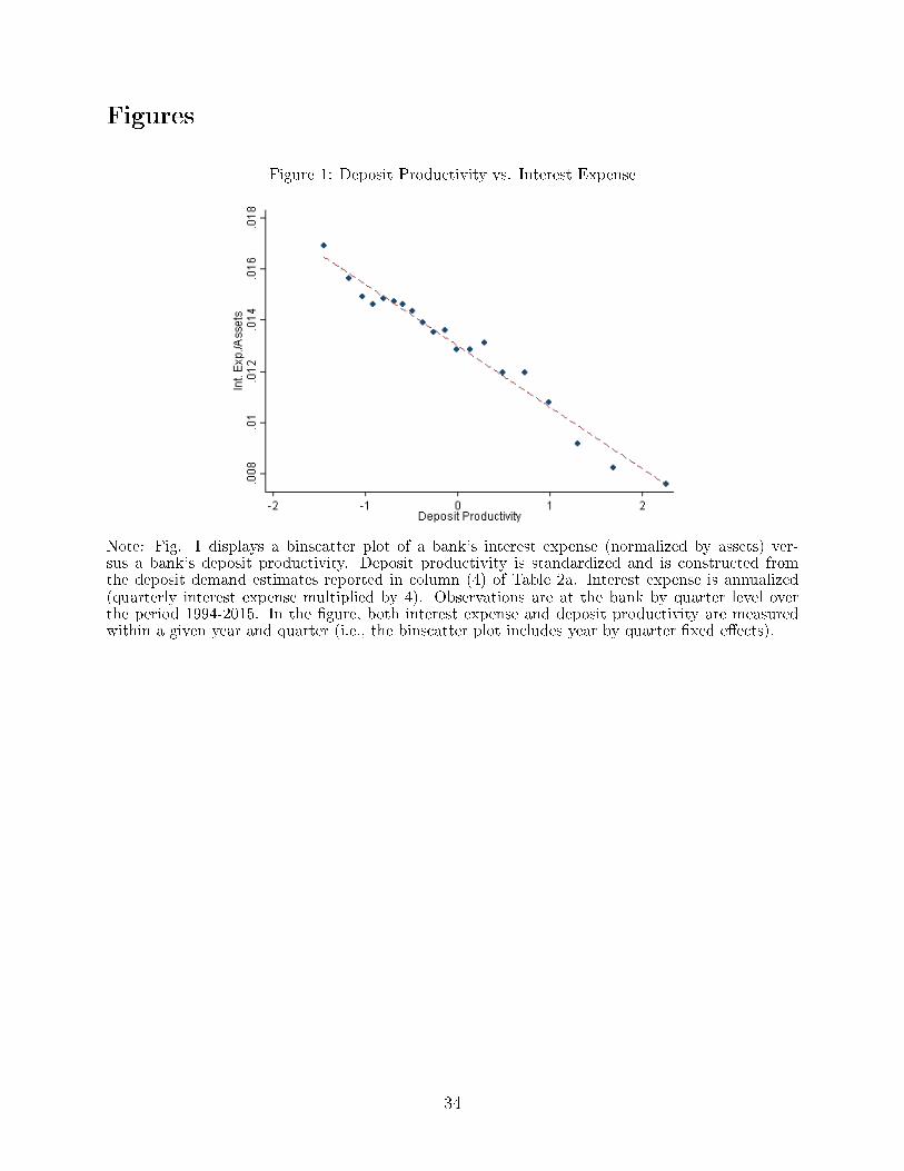
Figures

Figure 1: Deposit Productivity vs. Interest Expense

Note: Fig. 1 displays a binscatter plot of a bank's interest expense (normalized by assets) ver-sus a bank's deposit productivity. Deposit productivity is standardized and is constructed fromthe deposit demand estimates reported in column (4) of Table 2a. Interest expense is annualized(quarterly interest expense multiplied by 4). Observations are at the bank by quarter level overthe period 1994-2015. In the �gure, both interest expense and deposit productivity are measuredwithin a given year and quarter (i.e., the binscatter plot includes year by quarter �xed e�ects).

34

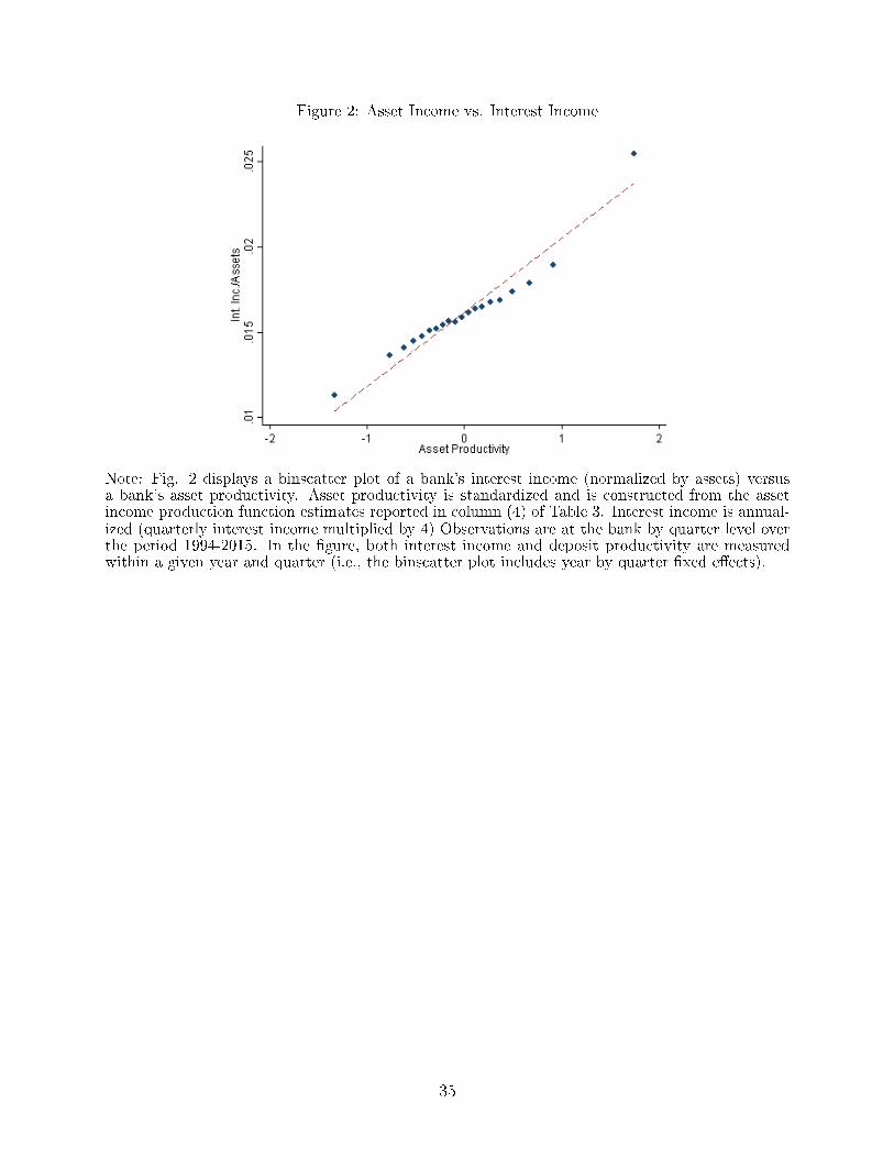
Figure 2: Asset Income vs. Interest Income

Note: Fig. 2 displays a binscatter plot of a bank's interest income (normalized by assets) versusa bank's asset productivity. Asset productivity is standardized and is constructed from the assetincome production function estimates reported in column (4) of Table 3. Interest income is annual-ized (quarterly interest income multiplied by 4) Observations are at the bank by quarter level overthe period 1994-2015. In the �gure, both interest income and deposit productivity are measuredwithin a given year and quarter (i.e., the binscatter plot includes year by quarter �xed e�ects).

35

Figure 3: Value Creation: Asset Productivity vs. Deposit Productivity

Note: Fig. 3 displays the estimated distributions of asset and deposit productivity. The red

shaded histogram plots the distribution of bank deposit productivity weighted by DepositsAssets

1α . The

blue histogram displays the scaled distribution of asset productivity Assetsθ

Assetsexp(φjt + ΓXjt). We

normalize the level of asset productivity relative to 3-month LIBOR such that the small set ofbanks earning returns below 3-month LIBOR have negative asset productivity. Similarly, we alsonormalize the deposit productivity distribution relative to 3-month LIBOR. We �nd that 16% ofbanks o�er deposit rates (net of fees) that are greater than 3-month LIBOR. We normalize thedeposit productivity distribution under the assumption that the bottom 16% of banks in terms ofdeposit productivity in each quarter do not generate any value on the deposit side of the bank. Thedeposit productivity estimates correspond to the speci�cation reported in column (4) of Table 2a.The asset productivity estimates correspond to speci�cation reported in column (4) of Table 3.

36

Figure 4: Interest Expense vs Interest Income

Note: Fig. 4 displays the distributions of deposit interest expense and interest income. The redshaded histogram plots the distribution of deposit interest expense divided by assets. The blueshaded histogram plots the distribution of interest income divided by assets. Both deposit interestexpense and interest income are annualized (multiplied by 4).

37

Figure 5: Deposit Productivity Share

Note: Fig. 5 displays the distribution of the deposit value share of each bank as de�ned in Eq.(11). The deposit value share re�ects the percentage of bank value that is generated by depositproductivity relative to asset productivity. We censor those observations with negative deposit valueshares at zero and those observations with deposit value shares greater than 1 at 1. The depositand asset productivity estimates correspond the speci�cations reported in columns (4) of Table 2aand Table 3.

38

Tables

Table 1: Summary Statistics

Variable Obs Mean Std. Dev. Min MaxDeposit Int. Expense 26,742 2.18% 1.34% 0.11% 6.53%Deposit Int. Expense (Net of Fees) 26,742 1.73% 1.36% -0.46% 6.16%Non Int. Expense (Millions) 26,742 142.44 517.53 1.27 3,662.00No. Branches 26,742 119.50 307.73 1.00 2,024.00No Employees 26,742 3,456.47 10,511.54 54.00 68,396.00Assets (Billions) 26,742 26.50 161.00 0.10 2,580.00Interest Income (Millions) 26,742 281.85 1,524.57 1.50 33,000.00Deposits (Billions) 26,742 14.20 78.90 0.01 1,370.00Leverage 26,742 0.91 0.04 0.19 1.02Beta 26,742 0.63 0.58 -0.66 2.46Std. Dev. ROA 26,742 0.14% 0.18% 0.01% 0.91%Market-to-Book 26,742 1.71 0.85 0.18 5.30Liabilities (Relative to Total Liabilities)

Deposits 26,742 0.83 0.13 0.00 1.00Small Time Deposits 26,736 0.20 0.11 0.00 0.68Large Time Deposits 26,736 0.13 0.08 0.00 0.89Savings Deposits 24,633 0.34 0.15 0.00 0.89Transaction Deposits 24,627 0.15 0.10 -0.30 0.81FF+Repo 18,051 0.04 0.06 0.00 0.69

Assets (Relative to Total Assets)Loans 26,742 0.65 0.13 0.00 0.96RE Loans 24,633 0.46 0.16 0.00 0.91C&I Loan 23,685 0.11 0.07 0.00 0.58Loan Commitments 26,742 0.14 0.17 0.00 21.10Securities 26,713 0.22 0.12 0.00 0.94Cash 26,732 0.02 0.04 0.00 0.41FF+Repo 18,047 0.01 0.03 0.00 0.45

Note: Table 1 reports the summary statistics for our sample. Observations are at the bank byquarter level over the period 1994-2015. Deposit interest expense and deposit interest expense netof fees are both annualized (multiplied by 4). The following variables are winsorized at the 1% level:Deposit Int. Expense, Deposit Int. Expense (Net of Fees), Non Int. Expense, No. Branches, NoEmployees, Assets, Interest Income Deposits, Leverage, Beta, Std. Dev. ROA.

39

Table 2: Deposit Demand

(a) Deposit Demand - Aggregate Level Demand

(1) (2) (3) (4)

Deposit Rate 12.61*** 11.53*** 44.35*** 20.88***(1.848) (4.331) (8.960) (4.620)

No. Branches (hundreds) 0.0405*** 0.0401*** 0.0540*** 0.0441***(0.00934) (0.00940) (0.0110) (0.00957)

No. Empl (thousands) 0.0271*** 0.0270*** 0.0297*** 0.0278***(0.00816) (0.00818) (0.00910) (0.00839)

Non-Int. Exp. (billions) -0.0886 -0.0845 -0.209* -0.120(0.101) (0.103) (0.114) (0.104)

Time Fixed E�ects X X X XBank Fixed E�ects X X X XIV-1 X XIV-2 X XObservations 26,742 26,742 26,742 26,742R-squared 0.981 0.981 0.976 0.981

(b) Deposit Demand - County Level Demand

(1) (2)

Deposit Rate 20.33 18.19**(13.59) (8.213)

No. of Branches (County Level) 0.184***(0.00398)

County×Year Fixed E�ects X XBank Fixed E�ects X XIV X XObservations 260,881 260,881R-squared 0.659 0.779

Note: We report our demand estimates (Eq. 6) in Tables 2a and 2b. In Table 2a, we de�ne themarket for deposits at the aggregate US by quarter level. The unit of observation is at the bankby quarter level over the period 1994 through 2015. The key independent variable of interest is thedeposit rate o�ered for each bank. We measure the deposit rate as the bank's quarterly depositinterest expense net of fees (scaled by 4) divided by the bank's level of deposits. Because of thepotential endogeneity of the deposit rate, we instrument for the deposit rate using two sets ofinstruments. We construct our �rst instrument (IV-1) as the estimated deposit rate from a bankspeci�c pass-through regression of deposit rates on 3-month LIBOR. We construct our secondinstrument (IV-2) as the average of the product characteristics o�ered by a bank's competitors inthe previous quarter (branches, employees, non-int expense, and fees). Speci�cally, we calculatethe average product characteristics of a bank's competitors in each county the bank operates inin a given year, and then we calculate the average across all counties the bank operates in. Wewinsorize all independent variables at the 1% to help control for outliers in the sample. Standarderrors are clustered by bank and are reported in parentheses. *,**, and *** indicate signi�cance atthe 10%, 5%, and 1% levels, respectively.

In Table 2b we de�ne the market for deposits at the county by year level. The unit of ob-servation is at the bank by county by year level over the period 2002 through 2012. We instrumentfor the deposit rate using the estimated deposit rate from a bank by county speci�c pass-throughregression of deposit rates on 3-month LIBOR. We winsorize all independent variables at the 1%to help control for outliers in the sample. Standard errors are clustered at the bank level andare reported in parentheses. *,**, and *** indicate signi�cance at the 10%, 5%, and 1% levels,respectively. 40

Table 3: Bank Production Function (Asset Income)

(1) (2) (3) (4) (5) (6)lnAkt (θ) 0.848*** 0.852*** 0.847*** 0.894*** 0.905*** 0.888***

(0.0132) (0.0133) (0.0143) (0.0361) (0.0354) (0.0379)Beta -0.00172 -0.00813 -0.00352 -0.00939

(0.00524) (0.00594) (0.00526) (0.00607)Beta (fwd 2 yr) 0.0164*** 0.0150***

(0.00503) (0.00514)SD ROA -0.0277*** -0.0258*** -0.0288*** -0.0266***

(0.00301) (0.00338) (0.00301) (0.00337)SD ROA (fwd 2 yr) 0.00213 0.000776

(0.00299) (0.00320)Bank F.E. X X X X X XTime F.E. X X X X X XIV X X XObservations 26,742 26,742 21,289 26,742 26,742 21,289R-squared 0.992 0.992 0.992 0.992 0.992 0.992

Note: We report our asset income production function estimates (Eq. 9) in Table 3. The unitof observation is at the bank by quarter level over the period 1994 through 2015. The dependentvariable is the logged value of interest income earned by the bank. The key independent variable ofinterest is the log value of a bank's assets lagged by one year. Because of the potential endogeneityof assets, we instrument for assets in columns (4)-(6). Speci�cally, we instrument for assets usingthe weighted average of the deposit product characteristics of a bank 's competitors as describedin Section 3.3. We also control for the bank's equity beta, standard deviation of return on assets(standardized), and leverage. We measure equity beta on a rolling basis using monthly equityreturns over the previous 24 months using data from CRSP and Kenneth French. We measure thestandard deviation of return on assets on a rolling basis using quarterly income statement/balancesheet data over the previous eight quarters. Standard errors are clustered at the bank level andare reported in parentheses. *,**, and *** indicate signi�cance at the 10%, 5%, and 1% levels,respectively.

41

Table 4: Market to Book vs. Bank Productivity

(1) (2) (3) (4) (5) (6)Deposit Productivity 0.236*** 0.496*** 0.207*** 0.452***

(0.0235) (0.0792) (0.0287) (0.0810)Asset Productivity 0.225*** 0.144*** 0.0878* 0.100***

(0.0523) (0.0373) (0.0529) (0.0377)Time F.E. X X X X X XOther Controls X X XObservations 26,742 26,742 26,742 26,742 26,742 26,742R-squared 0.420 0.453 0.378 0.436 0.424 0.458

Note: Table 4 displays the estimation results corresponding to a linear regression model (Eq.10).The dependent variable is the bank's market to book. The key independent variables of interestare deposit and asset productivity. Both deposit and asset productivity are standardized. Thedeposit productivity estimates correspond to speci�cation reported in column (4) of Table 2a. Theasset productivity estimates correspond to speci�cation reported in column (4) of Table 3. The unitof observation is at the bank by quarter level over the period 1994 through 2015. Other controlsinclude assets (lagged by one year), leverage (lagged by one quarter), three-month returns (laggedby one quarter), equity beta, and the standard deviation of return on assets. Standard errors areclustered at the bank level and are reported in parentheses. *,**, and *** indicate signi�cance atthe 10%, 5%, and 1% levels, respectively.

42

Table 5: Productivity vs. Composition of Assets and Liabilities

(a) Composition of Liabilities and Deposit Productivity

Dep. Var Leverage DepositsLiabilities

Small Time Dep.Liabilities

Large Time Dep.Liabilities

Savings Dep.Liabilities

Trans. Dep.Liabilities

FF+RepoLiabilities

(1) (2) (3) (4) (5) (6) (7)Deposit Prod. 0.0225* 1.773*** -0.347*** 0.137 1.354*** 0.432*** -0.320

(0.0127) (0.134) (0.126) (0.0834) (0.160) (0.106) (0.239)

Time F.E. X X X X X X XOther Controls X X X X X X XObservations 26,742 26,742 26,736 26,736 24,633 24,627 18,051R-squared 0.969 0.558 0.376 0.160 0.383 0.232 0.142

(b) Composition of Assets and Asset Productivity

Dep. Var LoansAssets

RE LoansAssets

C&I LoanAssets

Loan Commit.Assets

SecuritiesAssets

CashAssets

FF+RepoAssets

(1) (2) (3) (4) (5) (6) (7)Asset Prod. 0.675*** 0.348*** 0.157*** 0.0938*** -0.462*** -0.338*** -0.295***

(0.0522) (0.0479) (0.0454) (0.0234) (0.0483) (0.118) (0.113)

Time F.E. X X X X X X XOther Controls X X X X X X XObservations 26,742 24,633 23,685 26,742 26,713 26,732 18,047R-squared 0.288 0.353 0.057 0.134 0.147 0.235 0.116

Note: Table 5 panels (a) and (b) display the relationship between productivity and a bank's liabilityand asset structure. In Table 5a, we regress bank leverage and the composition of its deposits ondeposit productivity. We measure deposit productivity using the demand estimates reported incolumn (4) of Table 2a. In Table 5b, we regress the composition of a bank's assets on assetproductivity. We measure asset productivity using the estimates reported in column (4) of Table3. Observations in both Tables 5a and 5b are at the bank by quarter level over the period 1994-2015. Other controls include assets (lagged by one year), leverage (lagged by one quarter), three-month returns (lagged by one quarter), equity beta, and the standard deviation of return on assets.Standard errors are clustered at the bank level and are reported in parentheses. *,**, and ***indicate signi�cance at the 10%, 5%, and 1% levels, respectively.

43

Table 6: Deposit and Asset Productivity Subcategories

Dep. Var Deposit Productivity Asset Productivity Market to Book(1) (2) (3) (4) (5) (6)

Deposit Prod.:Savings 0.734*** 0.628*** 0.252*** 0.368***

(0.0279) (0.0422) (0.0360) (0.0535)Small Time 0.125*** 0.0945*** -0.228*** -0.180***

(0.0286) (0.0264) (0.0279) (0.0314)Large Time 0.179*** 0.156*** 0.0379 0.0724***

(0.0196) (0.0151) (0.0331) (0.0272)Transaction 0.414*** 0.371*** 0.0594* 0.104***

(0.0219) (0.0323) (0.0326) (0.0331)Asset Prod.:

Loans 0.166** 0.161** 0.0675** 0.0749**(0.0674) (0.0788) (0.0325) (0.0334)

Securities 0.0154 0.0159 0.0294 0.0697***(0.0147) (0.0235) (0.0244) (0.0244)

Time F.E. X X X X X XOther Controls X X XObservations 22,345 22,345 18,323 18,323 16,724 16,724R-squared 0.979 0.981 0.668 0.681 0.460 0.492

Note: Table 6 displays the relationship between our more re�ned measures of productivity, overallproductivity, and market to book. Overall deposit productivity is the dependent variable columns(1) and (2). We measure overall deposit productivity using the demand estimates reported incolumn (4) of Table 2a. Overall asset productivity is the dependent variable columns (3) and (4).We measure overall asset productivity using the production function estimates reported in column(4) of Table 3. Market-to-book is the dependent variable in columns (5) and (6). We measure depositproductivity for savings deposits, small time deposits, large deposits, and transaction deposits usingthe corresponding demand estimates reported in Table 7a. We measure asset productivity for loansand savings deposits using the corresponding production function estimates reported in Table 7b.Observations are at the bank by quarter level over the period 1994-2015. Other controls includeassets (lagged by one year), leverage (lagged by one quarter), three month returns (lagged by onequarter), equity beta, and sd of roa. Standard errors are clustered at the bank level and are reportedin parentheses. *,**, and *** indicate signi�cance at the 10%, 5%, and 1% levels, respectively.

44

Table 7: Re�ned Demand and Production Function Estimates

(a) Demand for Deposits by Type of Deposit

Deposit TypeSavings Small Time Large Time Transaction(1) (2) (3) (4)

Deposit Rate -9.594 63.17*** 75.39*** -1.188(12.73) (23.21) (18.25) (12.51)

No. Branches (hundreds) 0.0825*** 0.113*** 0.0265 0.0142(0.0211) (0.0412) (0.0263) (0.0143)

No. Empl (thousands) 0.00932 0.0241 0.0479*** 0.0377***(0.0102) (0.0185) (0.0135) (0.0104)

Non-Int. Exp. (billions) -0.192 -0.920*** -0.656*** 0.0724(0.154) (0.347) (0.247) (0.0881)

Time Fixed E�ects X X X XBank Fixed E�ects X X X XIV X X X XObservations 24,609 24,500 24,556 22,345R-squared 0.970 0.868 0.809 0.941

(b) Bank Production Function by Asset Type

Asset TypeLoans Securities(1) (2)

ln(Loanskt) (θL) 0.853***(0.0193)

ln(Securitieskt) (θS) 0.754***(0.0214)

Beta -0.0101 -0.00335(0.00618) (0.0104)

SD ROA -0.0303*** -0.0226***(0.00375) (0.00703)

Bank F.E. X XTime F.E. X XObservations 18,360 19,467R-squared 0.989 0.978

Note: Table 7a reports our baseline demand estimates for each type of deposit. The key independent variableof interest is the deposit rate o�ered for each bank. Because of the potential endogeneity of the deposit rate,we instrument for the deposit rate using two sets of instruments. We construct our �rst instrument (IV-1) as the estimated deposit rate from a bank speci�c pass-through regression of deposit rates on 3-monthLIBOR. We construct our second instrument (IV-2) as the average of the product characteristics o�ered bya bank's competitors in the previous quarter (branches, employees, non-int expense, and fees). Speci�cally,we calculate the average product characteristics of a bank's competitors in each county the bank operatesin in a given year ,and then we calculate the average across all counties the bank operates in. We winsorizeall independent variables at the 1% to help control for outliers in the sample. Standard errors are clusteredby bank and are reported in parentheses. *,**, and *** indicate signi�cance at the 10%, 5%, and 1% levels,respectively.Table 7b reports our asset production function estimates for loans and securities. The unit of observationis at the bank by quarter level over the period 1994 through 2015. The dependent variable in column (1)(column 2) is the logged value of loan (securities) interest income earned by the bank. The key independentvariable of interest in column (1) (column 2) is the log value of the bank loans (securities) lagged by oneyear. We also control for the bank's equity beta, standard deviation of return on assets (standardized),and leverage. We measure equity beta on a rolling basis using monthly equity returns over the previous 24months using data provided by CRSP and Kenneth French. We measure the standard deviation of returnon assets on a rolling basis using quarterly income statement/balance sheet data over the previous eightquarters. Standard errors are clustered at the bank level and are reported in parentheses. *,**, and ***indicate signi�cance at the 10%, 5%, and 1% levels, respectively.

45

Table 8: Deposit and Asset Synergies

Dep. Var Asset Productivity Loan Productivity Sec. Productivity(1) (2) (3) (4) (5) (6)

Deposit Productivity 0.328*** 0.441*** 0.504*** 0.340*** 0.692*** 0.0985(0.0304) (0.0937) (0.0543) (0.110) (0.0242) (0.0966)

Time F.E. X X X X X XOther Controls X X XObservations 26,742 26,742 18,360 18,360 19,467 19,467R-squared 0.630 0.644 0.409 0.420 0.612 0.647

Note: Table 8 displays the relationship between deposit productivity and asset productivity (eq.12). Each column corresponds to a separate linear regression. The dependent variable in columns(1)-(2) is overall productivity as measured using the production function estimates reported incolumn (4) of Table 3. The dependent variable in columns (3)-(4) is loan productivity as measuredusing the production function estimates reported in column (1) of Table 7b. The dependent variablein columns (5)-(6) is securities productivity as measured using the production function estimatesreported in column (2) of Table 7b. The key independent variable of interest is deposit productivity.We measure deposit productivity using the demand estimates reported in column (4) of Table 2a.Observations are at the bank by quarter level over the period 1994-2015. Other controls includeassets (lagged by one year), leverage (lagged by one quarter), three-month returns (lagged by onequarter), equity beta, and the standard deviation of return on assets. Standard errors are clusteredat the bank level and are reported in parentheses. *,**, and *** indicate signi�cance at the 10%,5%, and 1% levels, respectively.

46

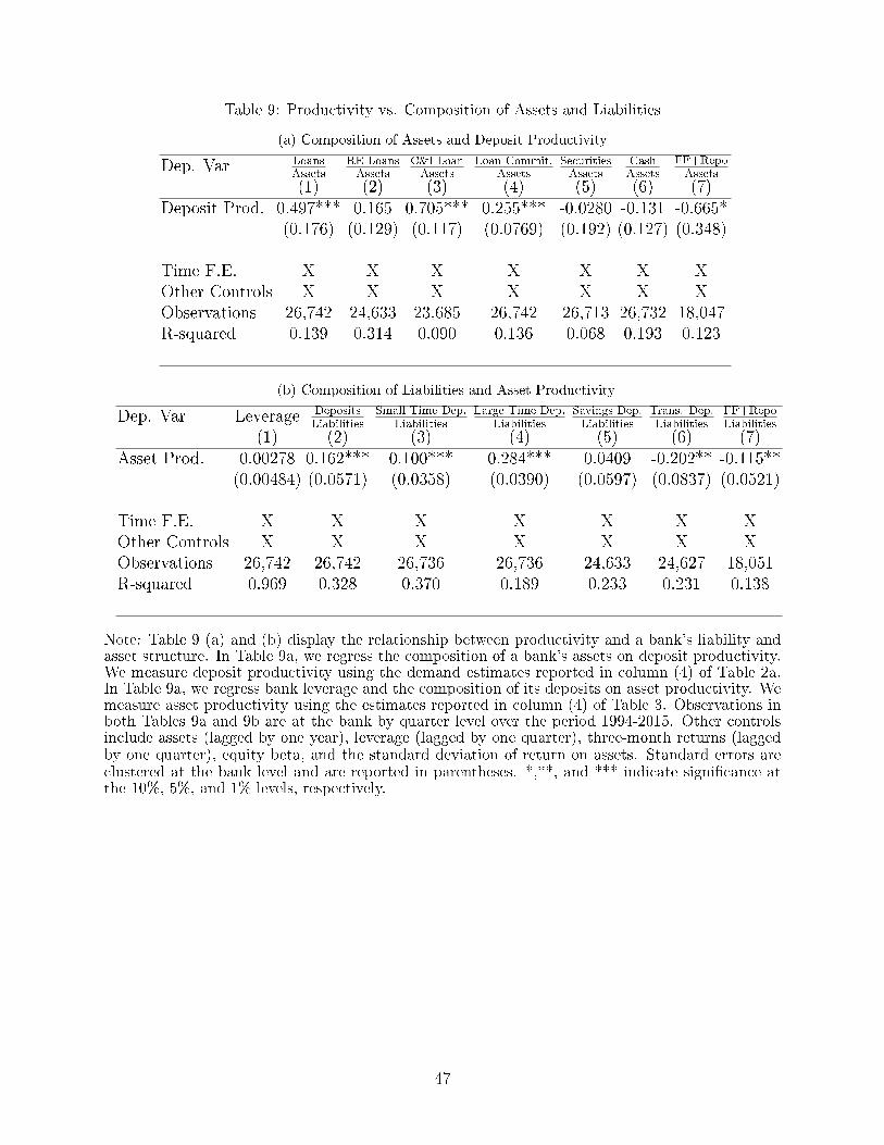
Table 9: Productivity vs. Composition of Assets and Liabilities

(a) Composition of Assets and Deposit Productivity

Dep. Var LoansAssets

RE LoansAssets

C&I LoanAssets

Loan Commit.Assets

SecuritiesAssets

CashAssets

FF+RepoAssets

(1) (2) (3) (4) (5) (6) (7)Deposit Prod. 0.497*** 0.165 0.705*** 0.255*** -0.0280 -0.131 -0.665*

(0.176) (0.129) (0.117) (0.0769) (0.192) (0.127) (0.348)

Time F.E. X X X X X X XOther Controls X X X X X X XObservations 26,742 24,633 23,685 26,742 26,713 26,732 18,047R-squared 0.139 0.314 0.090 0.136 0.068 0.193 0.123

(b) Composition of Liabilities and Asset Productivity

Dep. Var Leverage DepositsLiabilities

Small Time Dep.Liabilities

Large Time Dep.Liabilities

Savings Dep.Liabilities

Trans. Dep.Liabilities

FF+RepoLiabilities

(1) (2) (3) (4) (5) (6) (7)Asset Prod. 0.00278 0.162*** 0.100*** 0.284*** 0.0409 -0.202** -0.115**

(0.00484) (0.0571) (0.0358) (0.0390) (0.0597) (0.0837) (0.0521)

Time F.E. X X X X X X XOther Controls X X X X X X XObservations 26,742 26,742 26,736 26,736 24,633 24,627 18,051R-squared 0.969 0.328 0.370 0.189 0.233 0.231 0.138

Note: Table 9 (a) and (b) display the relationship between productivity and a bank's liability andasset structure. In Table 9a, we regress the composition of a bank's assets on deposit productivity.We measure deposit productivity using the demand estimates reported in column (4) of Table 2a.In Table 9a, we regress bank leverage and the composition of its deposits on asset productivity. Wemeasure asset productivity using the estimates reported in column (4) of Table 3. Observations inboth Tables 9a and 9b are at the bank by quarter level over the period 1994-2015. Other controlsinclude assets (lagged by one year), leverage (lagged by one quarter), three-month returns (laggedby one quarter), equity beta, and the standard deviation of return on assets. Standard errors areclustered at the bank level and are reported in parentheses. *,**, and *** indicate signi�cance atthe 10%, 5%, and 1% levels, respectively.

47

Appendix Figures and Tables

Figure A1: Value Creation: Asset Productivity vs. Deposit Productivity

Note: Fig. A1 displays the distributions of our empirical Bayes estimates of asset and depositproductivity as discussed in Section 5.2.2. Speci�cally, we "shrink" the estimated distribution ofasset and deposit productivity to account for measurement error. The the red shaded histogramplots the distribution of our empirical Bayes estimates of bank deposit productivity weighted byDepositsAssets

1α . The blue histogram displays the distribution of our empirical Bayes estimates of asset

productivity Assetsθ

Assetsexp(φjt+ΓXjt). We normalize the level of asset productivity relative to 3-month

LIBOR such that the small set of banks earning returns below 3-month LIBOR have negative assetproductivity. Similarly, we also normalize the deposit total factor productivity distribution relativeto 3-month LIBOR. We �nd that 16% of banks o�er net deposit rates (net of fees) that are greaterthan 3-month LIBOR. We normalize the deposit productivity distribution under the assumptionthat bottom 16% of banks in terms of deposit productivity in each quarter do not generate anyvalue on the deposit side of the bank. The deposit productivity estimates correspond to speci�cationreported in column (4) of Table 2a. The asset productivity estimates correspond to speci�cationreported in column (4) of Table 3.

48

Table A1: Alternative Asset Production Fuction Estimates

(a) Alternative Production Function Estimates - Spline

Dep. Var. Market to Book Asset Productivity(1) (2) (3) (4)

Deposit Productivity 0.242*** 0.343*** 0.553*** 0.451***(0.0363) (0.105) (0.0369) (0.131)

Asset Productivity 0.0281 0.118**(0.0516) (0.0459)

Time F.E. X X X XOther Controls X XObservations 21,362 21,362 21,362 21,362R-squared 0.413 0.454 0.655 0.705

(b) Alternative Production Function Estimates - Asset Composition

Dep. Var. Market to Book Asset Productivity(1) (2) (3) (4)

Deposit Productivity 0.222*** 0.500*** 0.374*** 0.351***(0.0373) (0.0955) (0.0336) (0.0846)

Asset Productivity 0.0939 0.107**(0.0627) (0.0440)

Time F.E. X X X XOther Controls X XObservations 18,564 18,564 18,564 18,564R-squared 0.429 0.463 0.654 0.666

Note: In Tables A1a and A1b, we replicate our baseline set of results using our alternative measuresof asset productivity. To construct the measure of asset productivity reported In Table A1a, weestimate the bank's asset income production function using a spline with �ve knot points as discussedin Section 5.1.1. To construct the measure of asset productivity reported In Table A1b, we estimatethe bank's asset income production function where we control for the Fama French risk factorsand the proportion of a bank's assets held in both loans and securities (both lagged by one year).We measure deposit productivity using the demand estimates reported in column (4) of Table2a. Observations in both Tables A1a and A1b are at the bank by quarter level over the period1994-2015. Other controls include assets (lagged by one year), leverage (lagged by one quarter),three-month returns (lagged by one quarter), equity beta, and the standard deviation of return onassets. Standard errors are clustered at the bank level and are reported in parentheses. *,**, and*** indicate signi�cance at the 10%, 5%, and 1% levels, respectively.

49

Table A2: Alternative Demand Estimates

(a) Alternative Demand Estimates - County Level Demand

Dep. Var. Market to Book Asset Productivity(1) (2) (3) (4)

Deposit Productivity 0.112*** 0.162** 0.317*** 0.471***(0.0345) (0.0812) (0.0241) (0.101)

Asset Productivity 0.108** 0.106**(0.0502) (0.0501)

Time F.E. X X X XOther Controls X XObservations 3,050 3,050 3,050 3,050R-squared 0.431 0.482 0.511 0.525

(b) Alternative Demand Estimates - Alternative Instruments

Dep. Var. Market to Book Asset Productivity(1) (2) (3) (4)

Deposit Productivity 0.218*** 0.435*** 0.314*** 0.180***(0.0277) (0.0672) (0.0302) (0.0654)

Asset Productivity 0.0910* 0.120***(0.0520) (0.0379)

Time F.E. X X X XOther Controls X XObservations 26,742 26,742 6,358 26,742R-squared 0.431 0.465 0.628 0.632

Note: In Tables A2a and A2b, we replicate our baseline set of results using our alternative measureof deposit productivity. In Table A2a, we measure deposit productivity using the demand estimatesreported in column (1) of Table 2b as described in Section 5.1.3. In Table A2b, we measure depositproductivity using the demand estimates reported in column (3) of Table 2a. Standard errorsare clustered at the bank level and are reported in parentheses. The asset productivity estimatescorrespond to speci�cation reported in column (4) of Table 3. Observations in Table A2a are atthe bank by year level over the period 1994-2015. Observations in Table A2b are at the bank byquarter level over the period 1994-2015. Other controls include assets (lagged by one year), leverage(lagged by one quarter), three-month returns (lagged by one quarter), equity beta, and the standarddeviation of return on assets. Standard errors are clustered at the bank level and are reported inparentheses. *,**, and *** indicate signi�cance at the 10%, 5%, and 1% levels, respectively.

50

Table A3: Measurement Error - Instrumental Variables

Dep. Var. Market to Book Asset Productivity(1) (2) (3) (4)

Deposit Productivity 0.205*** 0.513*** 0.353*** 0.567***(0.0301) (0.106) (0.0270) (0.108)

Asset Productivity 0.0128 0.0596(0.0427) (0.0435)

Time F.E. X X X XOther Controls X XIV X X X XObservations 16,724 16,724 22,345 22,345R-squared 0.428 0.469 0.624 0.640

Note: In Table A3, we replicate our baseline set of results using instrumental variables to addresspotential measurement error issues. Speci�cally, we instrument for deposit productivity using thesubcategory deposit productivity measures that we construct from the estimates reported in Table7a. Similarly, we instrument for asset productivity using the subcategory asset productivity thatwe construct from the estimates reported in Table 7b. We measure deposit and asset productivityusing the estimates reported in columns (4) of Table 2a and 3. Observations are at the bank byquarter level over the period 1994-2015. Other controls include assets (lagged by one year), leverage(lagged by one quarter), three-month returns (lagged by one quarter), equity beta, and the standarddeviation of return on assets. Standard errors are clustered at the bank level and are reported inparentheses. *,**, and *** indicate signi�cance at the 10%, 5%, and 1% levels, respectively.

51

Table A4: Subsample Analysis

(a) Subsample Analysis - Excluding the Largest Banks

Dep. Var. Market to Book Asset Productivity(1) (2) (3) (4)

Deposit Productivity 0.224*** 0.465*** 0.341*** 0.983***(0.0299) (0.124) (0.0210) (0.113)

Asset Productivity 0.0957 0.104***(0.0641) (0.0360)

Time F.E. X X X XOther Controls X XIV X X X XObservations 24,881 24,881 24,881 24,881R-squared 0.426 0.459 0.650 0.686

(b) Subsample Analysis - Excluding the Financial Crisis

Dep. Var. Market to Book Asset Productivity(1) (2) (3) (4)

Deposit Productivity 0.213*** 0.464*** 0.329*** 0.453***(0.0287) (0.0795) (0.0302) (0.0991)

Asset Productivity 0.107** 0.113***(0.0517) (0.0385)

Time F.E. X X X XOther Controls X XObservations 24,211 24,211 24,211 24,211R-squared 0.402 0.432 0.642 0.654

Note: In Tables A4a and A4b, we replicate our baseline set of results using di�erent subsets of thedata. In Table A4a, we replicate our baseline set of results where we exclude the largest banks fromour sample. Speci�cally, we drop all observations of those banks that appear among the top 5% ofthe sample in terms of assets at any point in time. In Table A4a, we replicate our baseline set ofresults where we exclude all observations from the years surrounding the �nancial crisis (years 2008and 2009). We measure deposit and asset productivity using the estimates reported in columns (4)of Table 2a and 3. Observations are at the bank by quarter level over the period 1994-2015. Othercontrols include assets (lagged by one year), leverage (lagged by one quarter), three-month returns(lagged by one quarter), equity beta, and the standard deviation of return on assets. Standard errorsare clustered at the bank level and are reported in parentheses. *,**, and *** indicate signi�canceat the 10%, 5%, and 1% levels, respectively.

52

Table A5: Alternative Deposit Demand Estimates - Extended Data Set

(1) (2) (3) (4)

Deposit Rate 13.66*** 8.943** 48.25*** 19.67***(1.721) (4.363) (9.091) (4.664)

No. Branches (hundreds) 0.0330*** 0.0328*** 0.0338*** 0.0320***(0.00955) (0.00949) (0.0100) (0.00925)

No. Empl (thousands) 0.0366*** 0.0345*** 0.0527*** 0.0403***(0.0109) (0.0111) (0.0117) (0.0106)

Non-Int. Exp. (billions) -0.163 -0.148 -0.254** -0.165(0.117) (0.117) (0.127) (0.115)

Time Fixed E�ects X X X XBank Fixed E�ects X X X XIV-1 X XIV-2 X XObservations 33,145 33,145 32,083 32,083R-squared 0.976 0.976 0.971 0.977

Note: We report our demand estimates (Eq. 6) in Table A5. Here we re-estimate demand usingour extended data set of over 32k bank by quarter observations. In our baseline demand estimates(Table 2), we restrict our data set to the 26,742 bank/quarter observations for which data is availableto estimate both deposit demand and the asset production function. The unit of observation is thenat the bank by quarter level over the period 1994 through 2015. We de�ne the market for deposits atthe aggreate US by quarter level. The key independent variable of interest is the deposit rate o�eredfor each bank. We measure the deposit rate as the bank's quarterly deposit interest expense net offees (scaled by 4) divided by the bank's level of deposits. Because of the potential endogeneity ofthe deposit rate, we instrument for the deposit rate using two sets of instruments. We construct our�rst instrument (IV-1) as the estimated deposit rate from a bank speci�c pass-through regressionof deposit rates on 3-month LIBOR. We construct our second instrument (IV-2) as the averageof the product characteristics o�ered by a bank's competitors in the previous quarter (branches,employees, non-int expense, and fees). Speci�cally, we calculate the average product characteristicsof a bank's competitors in each county the bank operates in in a given year, and then we calculatethe average across all counties the bank operates in. We winsorize all independent variables at the1% to help control for outliers in the sample. Standard errors are clustered by bank and are reportedin parentheses. *,**, and *** indicate signi�cance at the 10%, 5%, and 1% levels, respectively.

53

Table A6: Alternative Production Function Estimates

(1) (2)lnAkt (θ) 0.879*** 0.891***

(0.0369) (0.0547)θ1 -0.00276

(0.0447)θ2 -0.00527

(0.0326)θ3 0.0190

(0.0282)θ4 -0.108***

(0.0297)Beta -0.00656

(0.00500)Beta (fwd 2 yr) 0.0128**

(0.00499)SD ROA -0.0290***

(0.00299)SD ROA (fwd 2 yr) 0.00132

(0.00339)SMB (fwd 2 yr) 0.00407

(0.00269)HML (fwd 2 yr) -0.000365

(0.00259)Bank F.E. X XTime F.E. X XIV XObservations 26,742 18,564R-squared 0.992 0.993

Note: Table A6 displays our alternative production function estimates. The unit of observationis at the bank by quarter level over the period 1994 through 2015. The dependent variable is thelogged value of interest income earned by the bank. The key independent variable of interest is thelog value of a bank's assets lagged by one year. In column (1) we estimate a bank's asset productionfunction using a spline with �ve knot points (eq. 13) as described in Section 5.1.1. In column (2) weestimate a bank's asset production function using our basline log-linear speci�cation and instrumentfor assets using the weighted average of the deposit product characteristics of a bank 's competitorsas described in Section 3.3. In both speci�cations, we control for the bank's equity beta, standarddeviation of return on assets (standardized), and leverage. In column (2), we also control for theother Fama French Factors, HML and SMB. We measure equity beta, HML, and SMB on a rollingbasis using monthly equity returns over the previous 24 months using data provided by CRSP andKenneth French. We measure the standard deviation of return on assets on a rolling basis usingquarterly income statement/balance sheet data over the previous eight quarters. Standard errorsare clustered at the bank level and are reported in parentheses. *,**, and *** indicate signi�canceat the 10%, 5%, and 1% levels, respectively.

54