The cqFlow Model: Model description and course
65
Page 1 D:\cqflow-1.0\Documents\cqflow-course.sxi Fiesta Workshop June 29 – July 1 San Jose The cqFlow Model: Model description and course The Fiesta project J. Schellekens
Transcript of The cqFlow Model: Model description and course

Page 1 D:\cqflow-1.0\Documents\cqflow-course.sxi Fiesta Workshop June 29 – July 1 San Jose
The cqFlow Model:Model description and course
The Fiesta project
J. Schellekens

Page 2 D:\cqflow-1.0\Documents\cqflow-course.sxi Fiesta Workshop June 29 – July 1 San Jose
Updated files
Go to to 04 machine in the netwerk and find the share: CD\cqflow\updates
Copy the content of this directory to: d:\cqflow\cqflow-course(nb overwrite the existing files)
Also includes this presentation as pdf
Page 3 D:\cqflow-1.0\Documents\cqflow-course.sxi Fiesta Workshop June 29 – July 1 San Jose
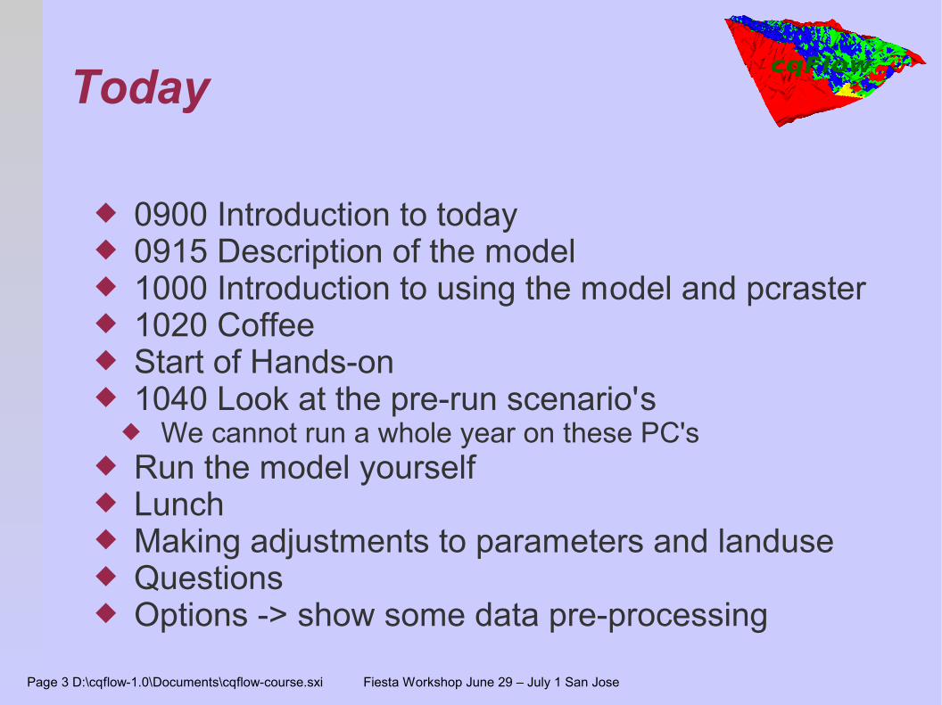
Today
0900 Introduction to today 0915 Description of the model 1000 Introduction to using the model and pcraster 1020 Coffee Start of Hands-on 1040 Look at the pre-run scenario's
We cannot run a whole year on these PC's Run the model yourself Lunch Making adjustments to parameters and landuse Questions Options -> show some data pre-processing

Page 4 D:\cqflow-1.0\Documents\cqflow-short.sxi Fiesta Workshop June 29 – July 1 San Jose
Why the cqFlow model? The main purpose of the cqFlow model is to
quantify the discharge from the Rio Chiquito catchment and evaluate the consequences of several land use scenarios within the catchment
As such, it can be used to: ...integrate the results from the plot scale and sub-basin
scale studies to a large scale ...evaluate the hydrological consequences of land use
change in this cloud forest catchment (scenario runs) In addition, the model is flexible enough to allow it
to be applied to other catchments later (re-calibration will be required)

Page 5 D:\cqflow-1.0\Documents\cqflow-short.sxi Fiesta Workshop June 29 – July 1 San Jose
cqFlow assumptions The catchment can be modelled using hourly time
steps Translation tables between land use and soil type
maps can be used to derive model parameters Fog interception can be modelled by aspect, wind
speed, wind direction and catching efficiency. Juvic gauge information is needed to determine HP.
Fog interception can be added as a surplus precipitation to an existing interception model by adding the volume of cloud water interception to the canopy store

Page 6 D:\cqflow-1.0\Documents\cqflow-short.sxi Fiesta Workshop June 29 – July 1 San Jose
Status of cqFlow
A running, calibrated model written in pcraster Simple command-line user interface Model description User manual -> September 2005 Requires expert knowledge
Will be available for download from the Fiesta web-site: http://www.geo.vu.nl/users/fiesta/
Presently available at:http://www.xs4all.nl/~schj/cqflow/
The version you are using is NOT the final version. Final version available in September
Page 7 D:\cqflow-1.0\Documents\cqflow-course.sxi Fiesta Workshop June 29 – July 1 San Jose
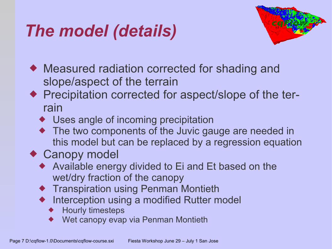
The model (details)
Measured radiation corrected for shading and slope/aspect of the terrain
Precipitation corrected for aspect/slope of the ter-rain
Uses angle of incoming precipitation The two components of the Juvic gauge are needed in
this model but can be replaced by a regression equation Canopy model
Available energy divided to Ei and Et based on the wet/dry fraction of the canopy
Transpiration using Penman Montieth Interception using a modified Rutter model
Hourly timesteps Wet canopy evap via Penman Montieth
Page 8 D:\cqflow-1.0\Documents\cqflow-course.sxi Fiesta Workshop June 29 – July 1 San Jose
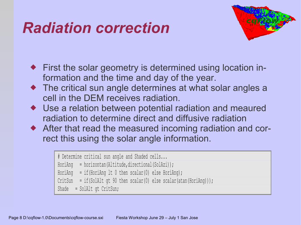
Radiation correction
First the solar geometry is determined using location in-formation and the time and day of the year.
The critical sun angle determines at what solar angles a cell in the DEM receives radiation.
Use a relation between potential radiation and meaured radiation to determine direct and diffusive radiation
After that read the measured incoming radiation and cor-rect this using the solar angle information.
# Determine critical sun angle and Shaded cells... HoriAng = horizontan(Altitude,directional(SolAzi)); HoriAng = if(HoriAng lt 0 then scalar(0) else HoriAng); CritSun = if(SolAlt gt 90 then scalar(0) else scalar(atan(HoriAng))); Shade = SolAlt gt CritSun;

Page 9 D:\cqflow-1.0\Documents\cqflow-course.sxi Fiesta Workshop June 29 – July 1 San Jose
Radiation correction
0
100
200
300
400
500
600
700
800
900
1000
0 5 10 15 20 25 30 35 40 45 50
Shortwave AVGCorrected SWPotential HOR

Page 10 D:\cqflow-1.0\Documents\cqflow-course.sxi Fiesta Workshop June 29 – July 1 San Jose
Radiation correction
0
50
100
150
200
250
300
0 50 100 150 200 250 300 350 400
Daily average catchment radiation
Measure shortwaveCorrected shortwave

Page 11 D:\cqflow-1.0\Documents\cqflow-course.sxi Fiesta Workshop June 29 – July 1 San Jose
Precipitation correction
The first step is to correct the gauge information for wind losses. This is a site/gauge specific function that should be re-determined when applying the model to another catchment.
Next the angle (in degrees from the vertical) of the incom-ing precipitation is determined using both components of the Juvic gauge
Alternatively a regression between speed and angle may be used
PCorrFac = 0.01 * exp(4.606 - 0.0057 * WindSpeed**2.0);Precipitation = Precipitation / PcorrFac;
Ratio = if (Precipitation > 0.0 then HP/Precipitation else 0.0);PrecipAngle = if (Precipitation == 0.0 then if (HP > 0.0 then 90 else 0.0) else scalar(atan(Ratio)))
Page 12 D:\cqflow-1.0\Documents\cqflow-course.sxi Fiesta Workshop June 29 – July 1 San Jose
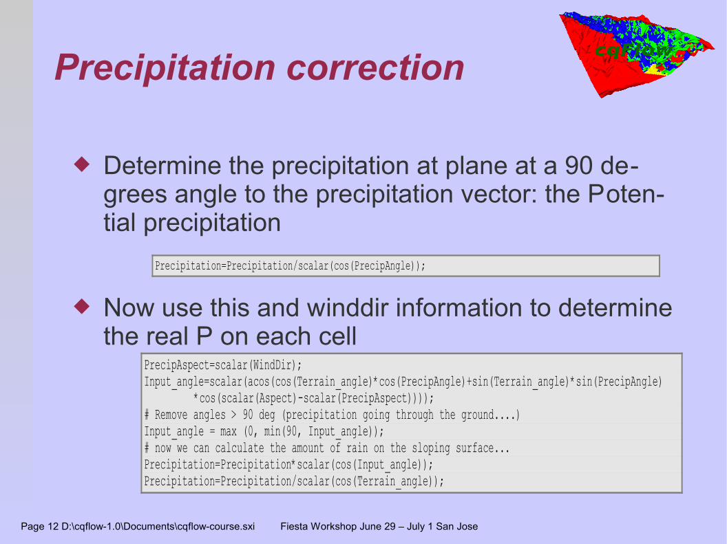
Precipitation correction
Determine the precipitation at plane at a 90 de-grees angle to the precipitation vector: the Poten-tial precipitation
Now use this and winddir information to determine the real P on each cell
Precipitation=Precipitation/scalar(cos(PrecipAngle));
PrecipAspect=scalar(WindDir);Input_angle=scalar(acos(cos(Terrain_angle)*cos(PrecipAngle)+sin(Terrain_angle)*sin(PrecipAngle)
*cos(scalar(Aspect)-scalar(PrecipAspect))));# Remove angles > 90 deg (precipitation going through the ground....)Input_angle = max (0, min(90, Input_angle));# now we can calculate the amount of rain on the sloping surface...Precipitation=Precipitation*scalar(cos(Input_angle));Precipitation=Precipitation/scalar(cos(Terrain_angle));
Page 13 D:\cqflow-1.0\Documents\cqflow-course.sxi Fiesta Workshop June 29 – July 1 San Jose
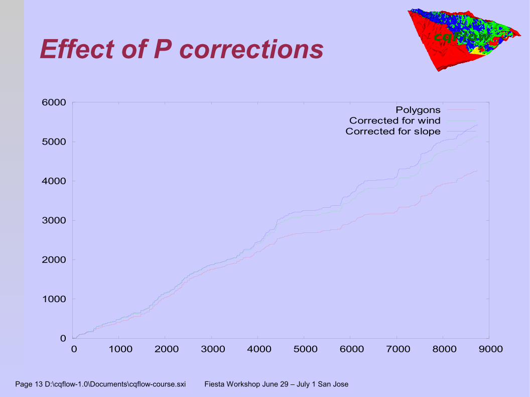
Effect of P corrections
0
1000
2000
3000
4000
5000
6000
0 1000 2000 3000 4000 5000 6000 7000 8000 9000
PolygonsCorrected for wind
Corrected for slope

Page 14 D:\cqflow-1.0\Documents\cqflow-course.sxi Fiesta Workshop June 29 – July 1 San Jose
Evapotranspiration (1)
Determine radiation using DEM and global incoming radiation. For this an existing model was adjusted.
Use measured radiation to scale the results Available energy determined using Albedo and a re-
gression equation for the Ground Heat Flux
Page 15 D:\cqflow-1.0\Documents\cqflow-course.sxi Fiesta Workshop June 29 – July 1 San Jose
Evapotranspiration (2)
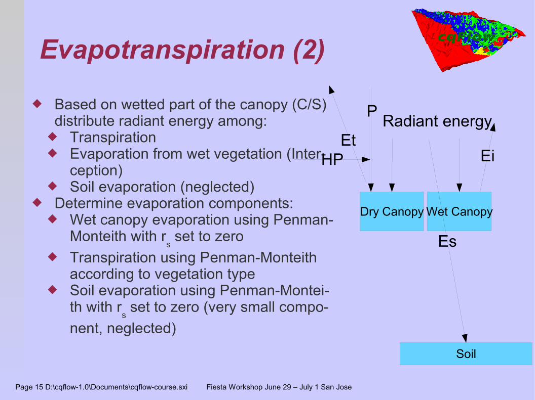
Based on wetted part of the canopy (C/S) distribute radiant energy among:
Transpiration Evaporation from wet vegetation (Inter-
ception) Soil evaporation (neglected)
Determine evaporation components: Wet canopy evaporation using Penman-
Monteith with rs set to zero
Transpiration using Penman-Monteith according to vegetation type
Soil evaporation using Penman-Montei-th with r
s set to zero (very small compo-
nent, neglected)
Dry Canopy Wet Canopy
Soil
Radiant energy
Es
EtEi
P
HP
Page 16 D:\cqflow-1.0\Documents\cqflow-course.sxi Fiesta Workshop June 29 – July 1 San Jose
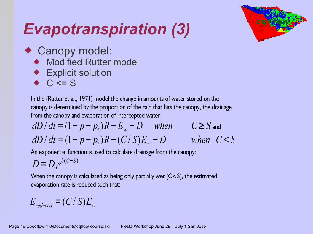
Evapotranspiration (3) Canopy model:
Modified Rutter model Explicit solution C <= S
In the (Rutter et al., 1971) model the change in amounts of water stored on the canopy is determined by the proportion of the rain that hits the canopy, the drainage from the canopy and evaporation of intercepted water:
dD dt p p R E D when C St w/ ( )= − − − − ≥1 and
dD dt p p R C S E D when C St w/ ( ) ( / )= − − − − <1An exponential function is used to calculate drainage from the canopy:
When the canopy is calculated as being only partially wet (C<S), the estimated evaporation rate is reduced such that:
D D eb C S= −0
( )
E C S Ereduced w= ( / )
Page 17 D:\cqflow-1.0\Documents\cqflow-course.sxi Fiesta Workshop June 29 – July 1 San Jose
The soil store Relatively simple but fully distributed conceptual model
based TOPOG_SBM model Implemented in Pcraster Uses a saturated and an unsaturated store

Page 18 D:\cqflow-1.0\Documents\cqflow-course.sxi Fiesta Workshop June 29 – July 1 San Jose
The soil
Inputs to the model: Et + Es from the canopy
model Total throughfall + stemflow
from the canopy model Determines:
In- exfiltration Lateral saturated flow Transfer between saturated
and unsaturated store Reduces Et + Es to an 'actual
evaporation' if water stress occurs (takes rooting depth into account).
Surface runoff via kinematic wave
U = TotalDepth - S
STotaldepth
transfer

Page 19 D:\cqflow-1.0\Documents\cqflow-course.sxi Fiesta Workshop June 29 – July 1 San Jose
The Soil
Ksat decreases expo-nentially in depth
Transfer between un-saturated and saturat-ed store based on K at that depth
Infiltration can include sub-cell parameters for % of compacted soil. Will be finished in September
U = TotalDepth - S
STotaldepth
transfer
Page 20 D:\cqflow-1.0\Documents\cqflow-course.sxi Fiesta Workshop June 29 – July 1 San Jose
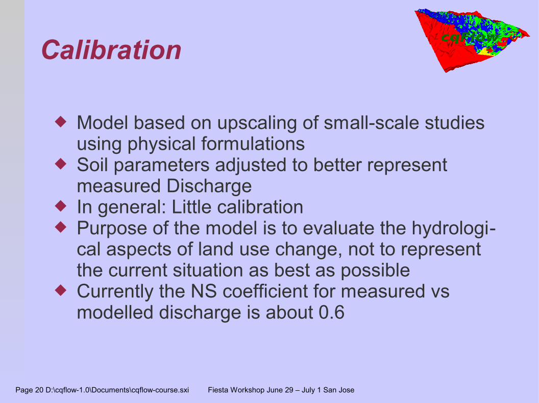
Calibration
Model based on upscaling of small-scale studies using physical formulations
Soil parameters adjusted to better represent measured Discharge
In general: Little calibration Purpose of the model is to evaluate the hydrologi-
cal aspects of land use change, not to represent the current situation as best as possible
Currently the NS coefficient for measured vs modelled discharge is about 0.6

Page 21 D:\cqflow-1.0\Documents\cqflow-course.sxi Fiesta Workshop June 29 – July 1 San Jose
How to deal with land-use change in a distributed model?
Use a GIS base programming language, pcraster Why pcraster?
Allows data centric modelling Allows you to work with distributed data relatively easily Simple programming language Fast implementation Free Can be used by a Msc student after a short introduction
This is needed to be able to handle the large amount of input data needed.

Page 22 D:\cqflow-1.0\Documents\cqflow-course.sxi Fiesta Workshop June 29 – July 1 San Jose
The cqFlow IT Implementation
Based on PCraster Dynamic GIS environment Rapid development, using freely available existing tools.
Perfect for use with distributed data. ArcView extensions available
penalty is speed (compared to C, C++, Fortan) PCraster extensions made for Fiesta in C
Needed when iteration is required (Rutter interception) Can help relieve the speed penalty Not used in the version we are using now
User interface via Matlab/Octave C routines to read/write PCraster maps Simple, fast and using standard tools
Easily adjustable by the user Free and (partly) open source software
Page 23 D:\cqflow-1.0\Documents\cqflow-course.sxi Fiesta Workshop June 29 – July 1 San Jose
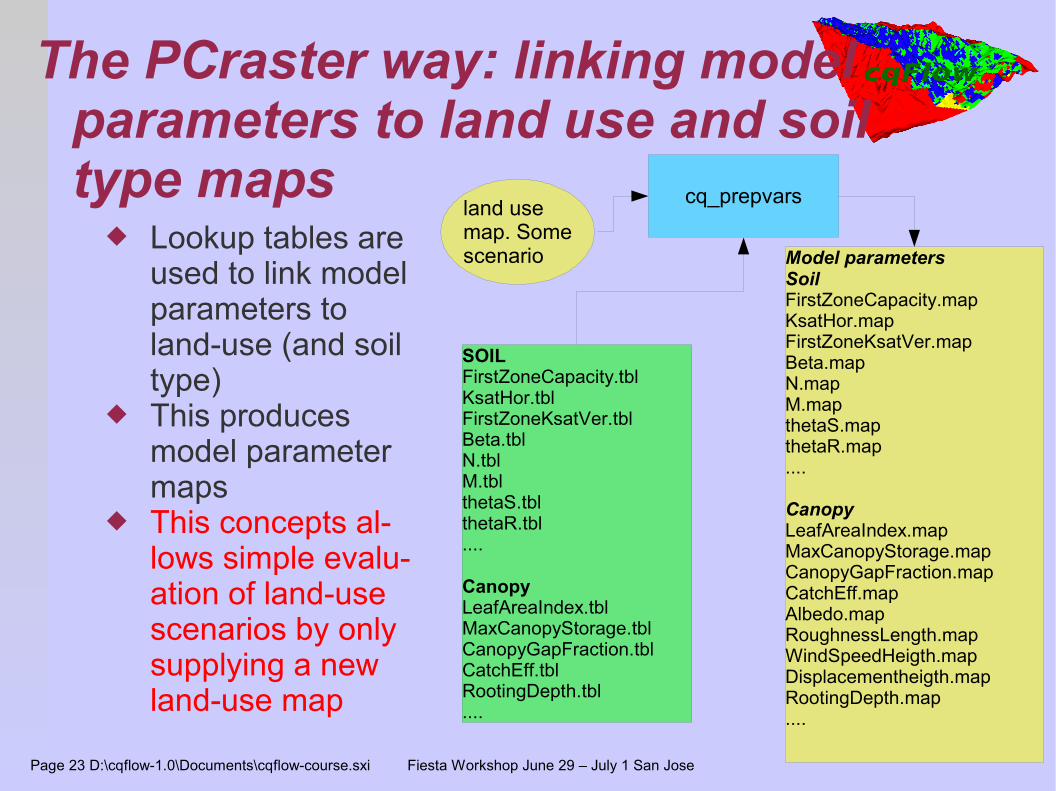
The PCraster way: linking model parameters to land use and soil type maps
Lookup tables are used to link model parameters to land-use (and soil type)
This produces model parameter maps
This concepts al-lows simple evalu-ation of land-use scenarios by only supplying a new land-use map
SOILFirstZoneCapacity.tblKsatHor.tblFirstZoneKsatVer.tblBeta.tblN.tblM.tblthetaS.tblthetaR.tbl....
CanopyLeafAreaIndex.tblMaxCanopyStorage.tblCanopyGapFraction.tblCatchEff.tblRootingDepth.tbl....
cq_prepvars
Model parametersSoilFirstZoneCapacity.mapKsatHor.mapFirstZoneKsatVer.mapBeta.mapN.mapM.mapthetaS.mapthetaR.map....
CanopyLeafAreaIndex.mapMaxCanopyStorage.mapCanopyGapFraction.mapCatchEff.mapAlbedo.mapRoughnessLength.mapWindSpeedHeigth.mapDisplacementheigth.mapRootingDepth.map....
land usemap. Somescenario
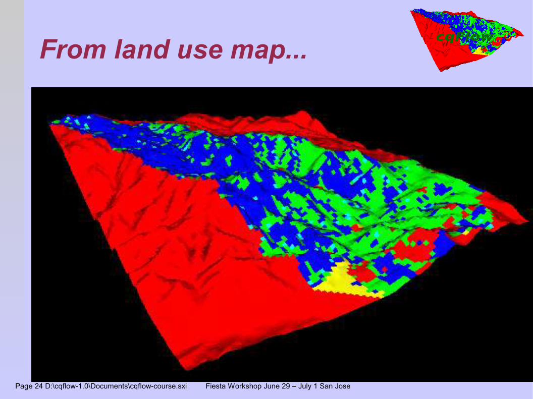
Page 24 D:\cqflow-1.0\Documents\cqflow-course.sxi Fiesta Workshop June 29 – July 1 San Jose
From land use map...
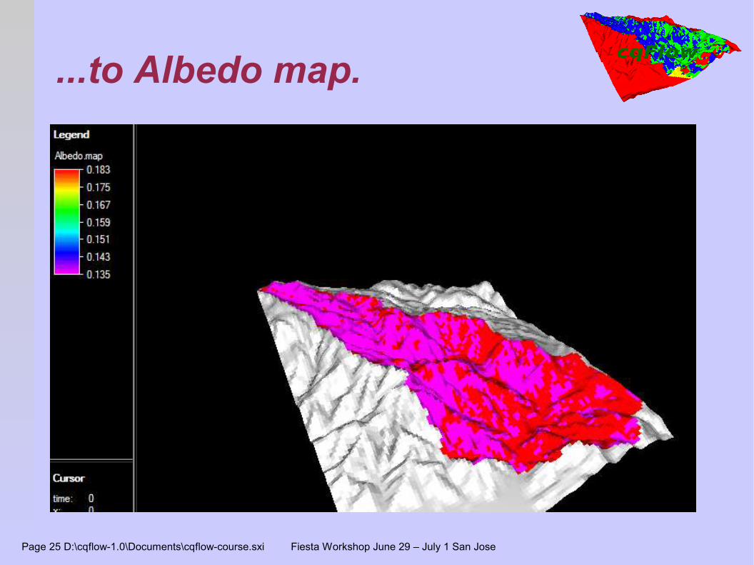
Page 25 D:\cqflow-1.0\Documents\cqflow-course.sxi Fiesta Workshop June 29 – July 1 San Jose
...to Albedo map.
Page 26 D:\cqflow-1.0\Documents\cqflow-course.sxi Fiesta Workshop June 29 – July 1 San Jose
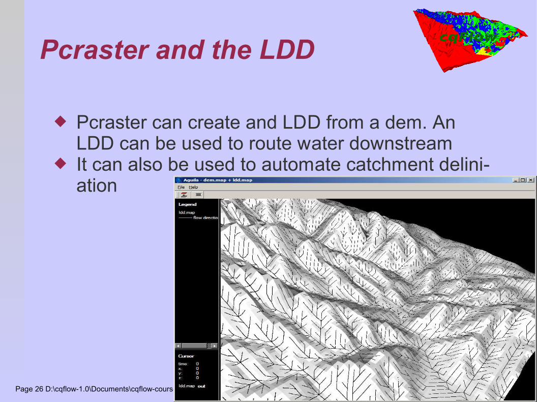
Pcraster and the LDD
Pcraster can create and LDD from a dem. An LDD can be used to route water downstream
It can also be used to automate catchment delini-ation
Page 27 D:\cqflow-1.0\Documents\cqflow-course.sxi Fiesta Workshop June 29 – July 1 San Jose
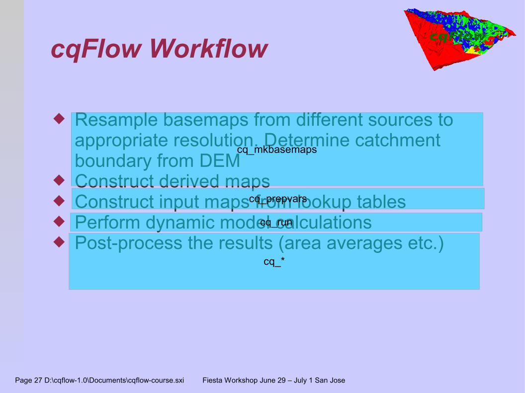
cqFlow Workflow
Resample basemaps from different sources to appropriate resolution. Determine catchment boundary from DEM
Construct derived maps Construct input maps from lookup tables Perform dynamic model calculations Post-process the results (area averages etc.)
cq_mkbasemaps
cq_prepvars
cq_run
cq_*
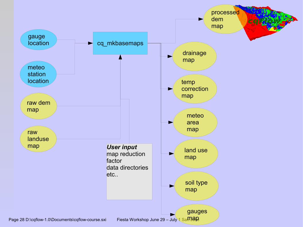
Page 28 D:\cqflow-1.0\Documents\cqflow-course.sxi Fiesta Workshop June 29 – July 1 San Jose
cq_mkbasemapsgauge location
raw demmap
meteostation location
raw landusemap
processeddemmap
drainagemap
temp correctionmap
meteoareamap
land usemap
soil typemap
gaugesmap
User inputmap reduction factordata directoriesetc..
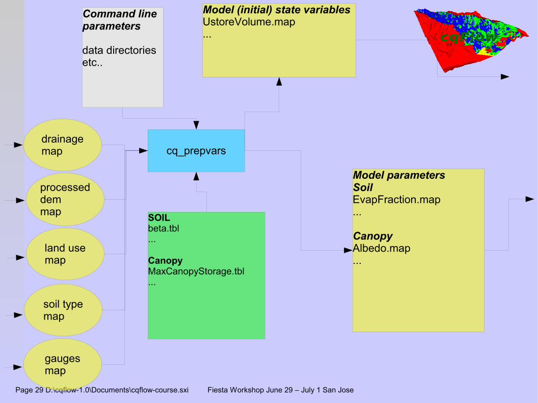
Page 29 D:\cqflow-1.0\Documents\cqflow-course.sxi Fiesta Workshop June 29 – July 1 San Jose
cq_prepvarsdrainagemap
land usemap
soil typemap
processeddemmap
gaugesmap
SOILbeta.tbl...
CanopyMaxCanopyStorage.tbl...
Model parametersSoilEvapFraction.map...
CanopyAlbedo.map...
Model (initial) state variablesUstoreVolume.map...
Command line parameters
data directoriesetc..

Page 30 D:\cqflow-1.0\Documents\cqflow-course.sxi Fiesta Workshop June 29 – July 1 San Jose
cq_runModel parameters
LeafAreaIndex.mapMaxCanopyStorage.mapCanopyGapFraction.mapCatchEff.mapAlbedo.map
Model (initial) state variablesSoilMoisture.map
CanopyStorage.map
temp correctionmap
meteoareamap
Timeseriesrain.tsstemp.tsswindspeed.tsswinddir.tssrh.tssradiation.tss
Results Time-series(average, and at selected points)...
Model state vari-ablesat end of run...
Model results (maps)...
Command line parameterstimestepsdata directoriesetc..
Page 31 D:\cqflow-1.0\Documents\cqflow-course.sxi Fiesta Workshop June 29 – July 1 San Jose
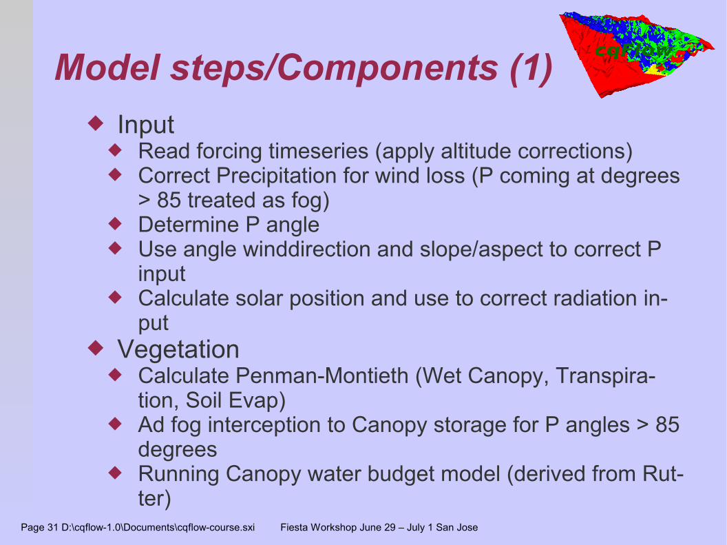
Model steps/Components (1) Input
Read forcing timeseries (apply altitude corrections) Correct Precipitation for wind loss (P coming at degrees
> 85 treated as fog) Determine P angle Use angle winddirection and slope/aspect to correct P
input Calculate solar position and use to correct radiation in-
put Vegetation
Calculate Penman-Montieth (Wet Canopy, Transpira-tion, Soil Evap)
Ad fog interception to Canopy storage for P angles > 85 degrees
Running Canopy water budget model (derived from Rut-ter)

Page 32 D:\cqflow-1.0\Documents\cqflow-course.sxi Fiesta Workshop June 29 – July 1 San Jose
Model steps/Components (2)
Soil Infiltration into unsat zone Et extraction via rooting depth (First from unsat zone; if
demand not met try Sat zone taking into account rooting depth)
Deep percolation (leakage) Transfer water from Unsat to Sat store Lateral transport of saturated water via Darcy Return flow to surface water Runoff via kinematic wave
Page 33 D:\cqflow-1.0\Documents\cqflow-course.sxi Fiesta Workshop June 29 – July 1 San Jose
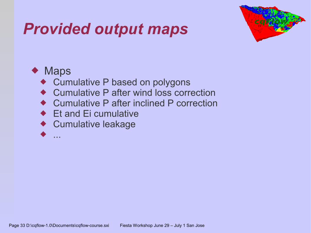
Provided output maps
Maps Cumulative P based on polygons Cumulative P after wind loss correction Cumulative P after inclined P correction Et and Ei cumulative Cumulative leakage ...

Page 34 D:\cqflow-1.0\Documents\cqflow-course.sxi Fiesta Workshop June 29 – July 1 San Jose
Scenarios
1. Scenarios1. Current land-use (baseline, used for limited calibration)2. Land use of 1975 landsat image; mostly forest3. Conversion of all land to pasture4. Conversion of all land above 1400m to pasture
2. Options1. HP Catching efficiency of pasture is 15 %2. HP Catching efficiency of pasture is 10 %3. HP Catching efficiency of pasture is 5 %
3. Subcatchment1. All the combinations above for a 11km^2 subcatchment
with outlet at 1321 m. This is a cloud forest catchment

Page 35 D:\cqflow-1.0\Documents\cqflow-course.sxi Fiesta Workshop June 29 – July 1 San Jose
Cloud forest sub catchment
Page 36 D:\cqflow-1.0\Documents\cqflow-course.sxi Fiesta Workshop June 29 – July 1 San Jose
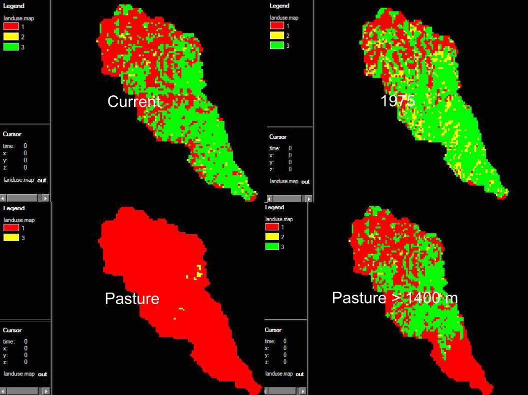
Pasture > 1400 m
Current 1975
Pasture
Page 37 D:\cqflow-1.0\Documents\cqflow-course.sxi Fiesta Workshop June 29 – July 1 San Jose
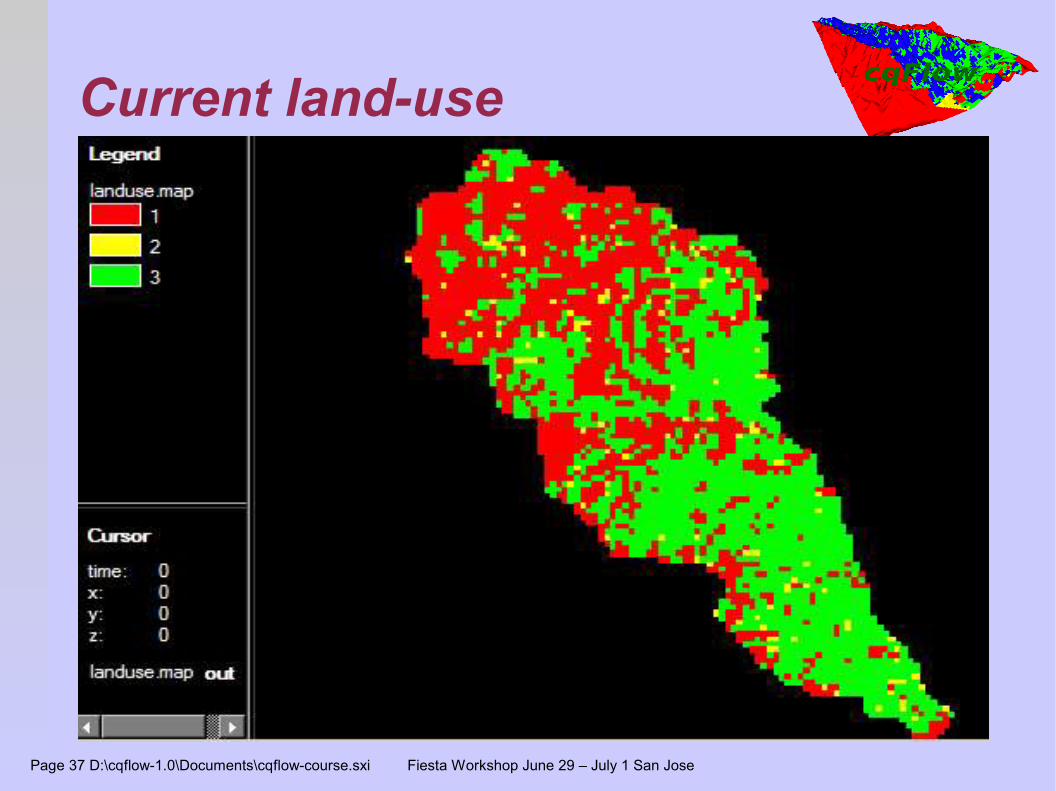
Current land-use
Used to check how well the model can predict current streamflow
Used for limited calibration Used to compare the other scenario's with Based on 2001 classified LandSat map
Pasture Secondary forest Primary forest

Page 38 D:\cqflow-1.0\Documents\cqflow-course.sxi Fiesta Workshop June 29 – July 1 San Jose
Summary of results
Current land useCatchEff Catchment P HP Et Ei Q Leakage Storage OutflowPasture mm mm % of P mm mm mm mm mm % of P
0,05 Whole 5429 246 4,53 751 284 3714 891 35 85,470,1 Whole 5429 282 5,19 750 286 3743 896 36 86,11
0,15 Whole 5429 318 5,86 750 287 3773 900 37 86,760,05 SubCatch 4697 767 16,33 536 328 3533 1022 45 97,93
0,1 SubCatch 4697 795 16,93 537 329 3551 1028 47 98,490,15 SubCatch 4697 823 17,52 537 329 3571 1034 49 99,08
For the whole catchment HP is less than 6% if the P input
However, for a sub-catchment > 1321 m this increas-es to 16 %
At the same time Et + Ei is smaller in the cloud forest resulting in more outflow of water
Page 39 D:\cqflow-1.0\Documents\cqflow-course.sxi Fiesta Workshop June 29 – July 1 San Jose
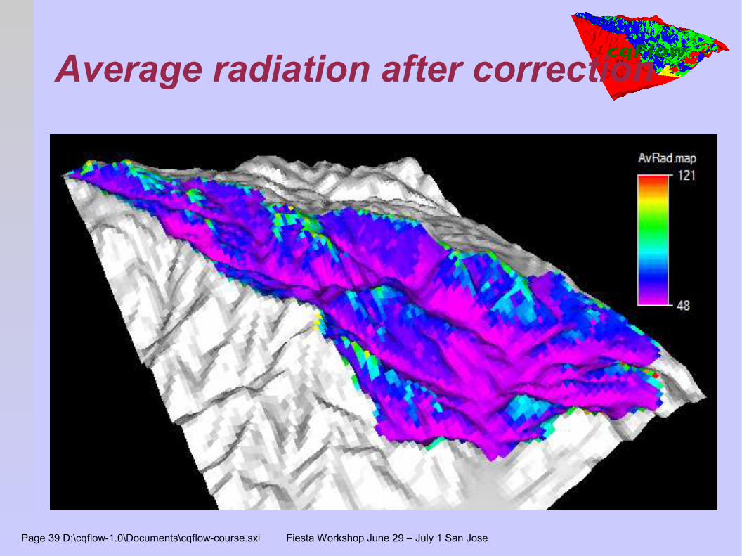
Average radiation after correction
Page 40 D:\cqflow-1.0\Documents\cqflow-course.sxi Fiesta Workshop June 29 – July 1 San Jose
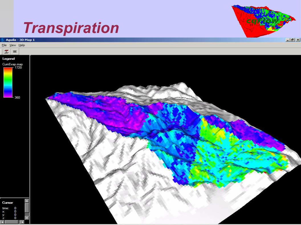
Transpiration
Page 41 D:\cqflow-1.0\Documents\cqflow-course.sxi Fiesta Workshop June 29 – July 1 San Jose
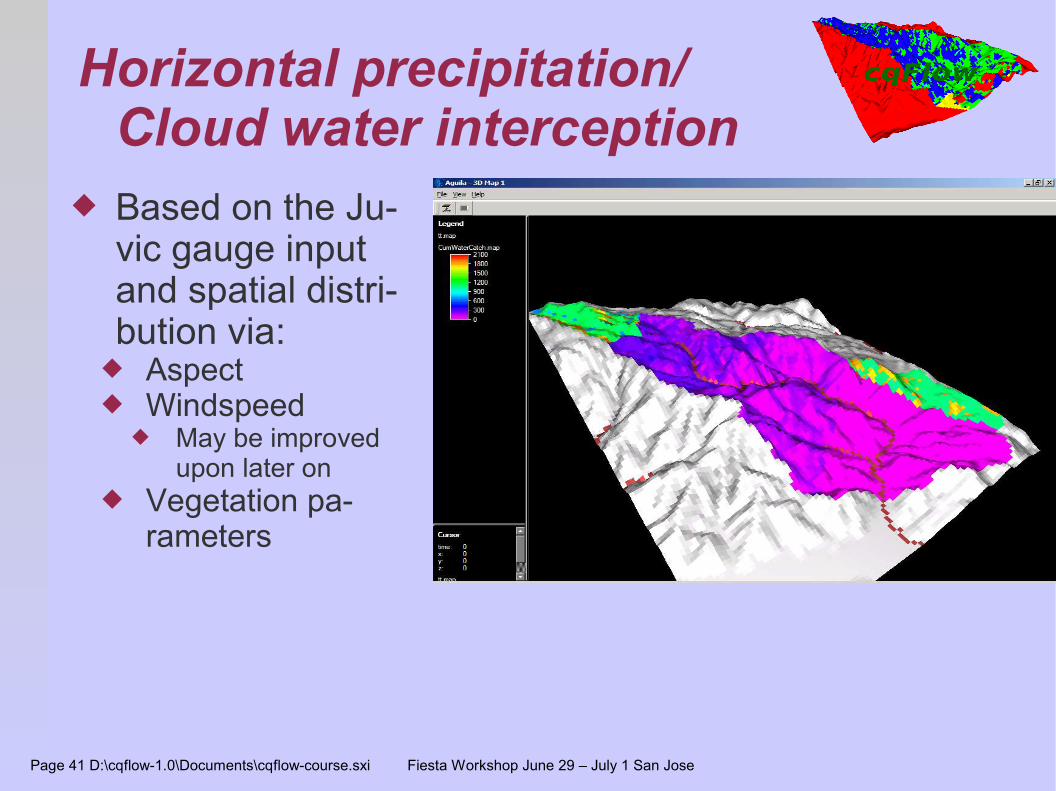
Horizontal precipitation/Cloud water interception
Based on the Ju-vic gauge input and spatial distri-bution via:
Aspect Windspeed
May be improved upon later on
Vegetation pa-rameters

Page 42 D:\cqflow-1.0\Documents\cqflow-course.sxi Fiesta Workshop June 29 – July 1 San Jose
Soil water
1600 1650 1700 1750 1800 1850 1900 1950
0 1000 2000 3000 4000 5000 6000 7000 8000 9000 1600 1650 1700 1750 1800 1850 1900 1950
Storage/runoff plot for run: default
Saturated store
150
200
250
300
350
400
450
0 1000 2000 3000 4000 5000 6000 7000 8000 9000 150
200
250
300
350
400
450Unsaturated Store

Page 43 D:\cqflow-1.0\Documents\cqflow-course.sxi Fiesta Workshop June 29 – July 1 San Jose
Hands-on
Using the model...

Page 44 D:\cqflow-1.0\Documents\cqflow-course.sxi Fiesta Workshop June 29 – July 1 San Jose
How to run the model?
Use the pcrshell environment This is basically a DOS box in which you type com-
mands NB A linux version of pcraster is also available
Use the nutshell environment Use Octave/Matlab as a shell
A simple interface has been set up in Octave Advantage -> powerfull processing Disadvantage -> need to learn Matlab/Octave
Pcraster models can also be run from within Ar-cView provided you have spatial analist and have the pcraster ArcView extension
Not set up for this course
Page 45 D:\cqflow-1.0\Documents\cqflow-course.sxi Fiesta Workshop June 29 – July 1 San Jose
How to install
Download pcraster from http://www.pcraster.nl Also download the update for pcraster Download nutshell (link at pcraster site) Download mapedit (link at pcraster site)
Install pcraster using the setup Copy the updated pcraster files to \pcraster\apps Install nutshell using the setup Copy mapedit.exe \pcraster\apps
Page 46 D:\cqflow-1.0\Documents\cqflow-course.sxi Fiesta Workshop June 29 – July 1 San Jose
How to view results
Maps Static maps -> display or aguila Timeseries of maps (mapstacks) -> display or aguila;
may use animation Time series
Timeplot Read into Matlab/octave and use plot Import into Excel
Viewing can also be used from within Nutshell In windows link .map files to display and .tss files
to timplot
Page 47 D:\cqflow-1.0\Documents\cqflow-course.sxi Fiesta Workshop June 29 – July 1 San Jose
What we will do Start up nutshell Display timeseries Display maps In addition we will look at the project scenario runs us-
ing nutshell
Run the default model Edit a landuse map using mapedit for myrun Re-run the model Compare results with previous run Adjust some model parameters and re-run the model
We will run 240 timsteps (hours) and not a full year because this takes to long (The P input in the exam-ples has been edited)

Page 48 D:\cqflow-1.0\Documents\cqflow-course.sxi Fiesta Workshop June 29 – July 1 San Jose
NutshellTree for navigation, shows the work-dir. Set the workdir in the treeview to the model you want to run
List of files. Select dem.map and set the aguila basemap(needed for 3D maps)
Page 49 D:\cqflow-1.0\Documents\cqflow-course.sxi Fiesta Workshop June 29 – July 1 San Jose
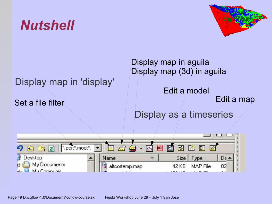
Nutshell
Display as a timeseries
Display map in 'display'
Display map in aguilaDisplay map (3d) in aguila
Edit a mapSet a file filterEdit a model
Page 50 D:\cqflow-1.0\Documents\cqflow-course.sxi Fiesta Workshop June 29 – July 1 San Jose
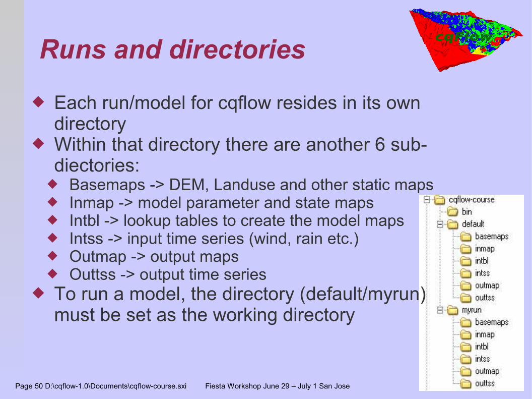
Runs and directories
Each run/model for cqflow resides in its own directory
Within that directory there are another 6 sub-diectories:
Basemaps -> DEM, Landuse and other static maps Inmap -> model parameter and state maps Intbl -> lookup tables to create the model maps Intss -> input time series (wind, rain etc.) Outmap -> output maps Outtss -> output time series
To run a model, the directory (default/myrun) must be set as the working directory
Page 51 D:\cqflow-1.0\Documents\cqflow-course.sxi Fiesta Workshop June 29 – July 1 San Jose
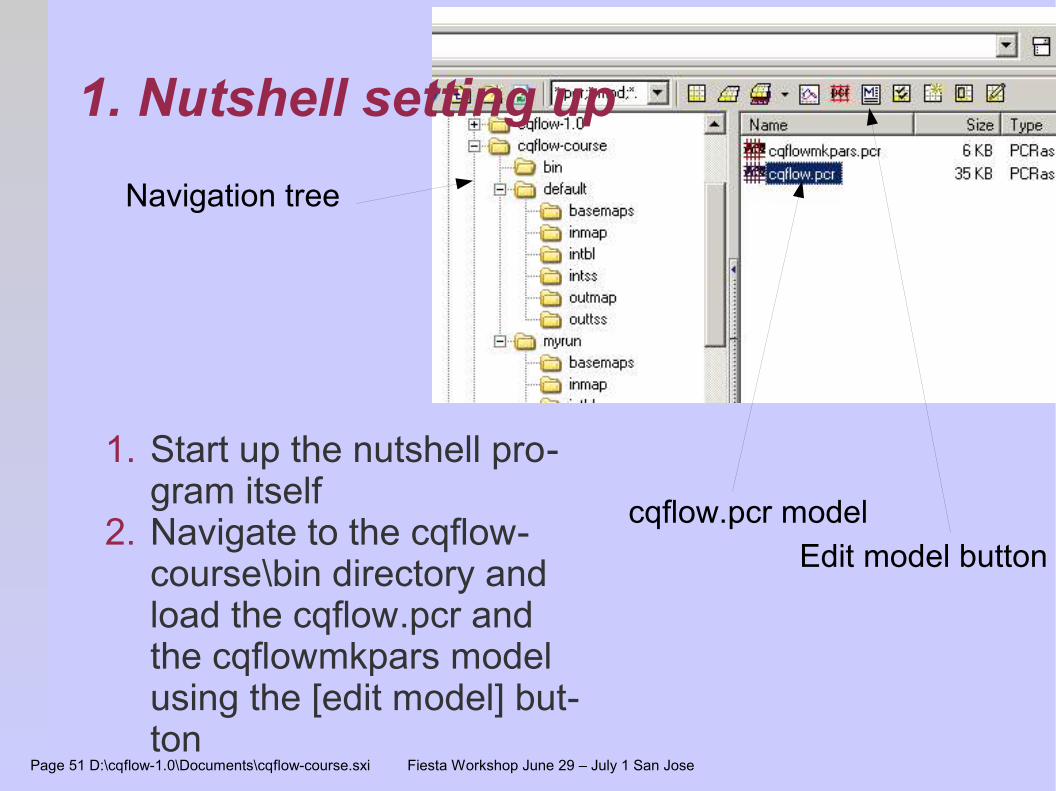
1. Nutshell setting up
1. Start up the nutshell pro-gram itself
2. Navigate to the cqflow-course\bin directory and load the cqflow.pcr and the cqflowmkpars model using the [edit model] but-ton
cqflow.pcr modelEdit model button
Navigation tree
Page 52 D:\cqflow-1.0\Documents\cqflow-course.sxi Fiesta Workshop June 29 – July 1 San Jose
2. Looking at the resultstime series
The results of the model run are saved in the outtss (time series) and outmap (maps) directory of the cqflow-results dir
Navigate to the outtss directory and make graphs of at least the following time series:
DischargeCubic.txt Evaporation.txt WaterCatch.txt -> Cloud water interception
To compare scenario's first open the .tss.,txt in the first scenario by selecting it and using the timeplot button. After that use the open column file. Do this for the default and deforestation sce-nario's
Also check out a few others (e.g. ActualStorage)

Page 53 D:\cqflow-1.0\Documents\cqflow-course.sxi Fiesta Workshop June 29 – July 1 San Jose
3. Looking at the resultsSingle maps
Output maps are stored in the outmap dir of each scenario Display the map CumEvap.map (Cumulative evaporation)
by either double clicking on it or by selecting it and press-ing the display button. Do this for at least two scenario's and compare the maps
Repeat this for a number of maps of interest
Also display some of the maps in the basemaps directory (e.g. lan-duse.map, dem.map...)
Page 54 D:\cqflow-1.0\Documents\cqflow-course.sxi Fiesta Workshop June 29 – July 1 San Jose
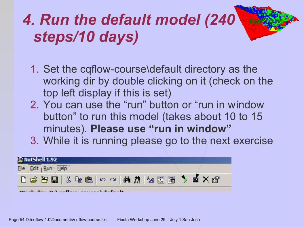
4. Run the default model (240 steps/10 days)
1. Set the cqflow-course\default directory as the working dir by double clicking on it (check on the top left display if this is set)
2. You can use the “run” button or “run in window button” to run this model (takes about 10 to 15 minutes). Please use “run in window”
3. While it is running please go to the next exercise
Page 55 D:\cqflow-1.0\Documents\cqflow-course.sxi Fiesta Workshop June 29 – July 1 San Jose
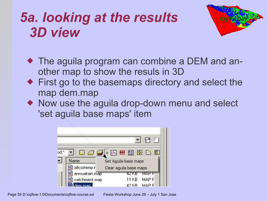
5a. looking at the results3D view
The aguila program can combine a DEM and an-other map to show the resuls in 3D
First go to the basemaps directory and select the map dem.map
Now use the aguila drop-down menu and select 'set aguila base maps' item
Page 56 D:\cqflow-1.0\Documents\cqflow-course.sxi Fiesta Workshop June 29 – July 1 San Jose
5b. Looking at the results3D view
After the basemap has been selected you can show any map in 3D
To do this select a map and use the aguila 3D button to show a map in 3D
Do this for a number of maps NB In aguila you can use the arrow keys to alter
the 3D view The FirstZoneDepth.map clearly shows the rela-
tion between topography and (shallow) groundwa-ter

Page 57 D:\cqflow-1.0\Documents\cqflow-course.sxi Fiesta Workshop June 29 – July 1 San Jose
6. Looking at the resultsmap series
Wait for the run to finish Go to the outmap directory Select the map series filter from the filter box Select a map series
Q = discharge ET = evaporation PR = Solar radiation WC = Cloud water interception
Use the display button to display the series In the display program use the animate button to
make a movie of the map series
Page 58 D:\cqflow-1.0\Documents\cqflow-course.sxi Fiesta Workshop June 29 – July 1 San Jose
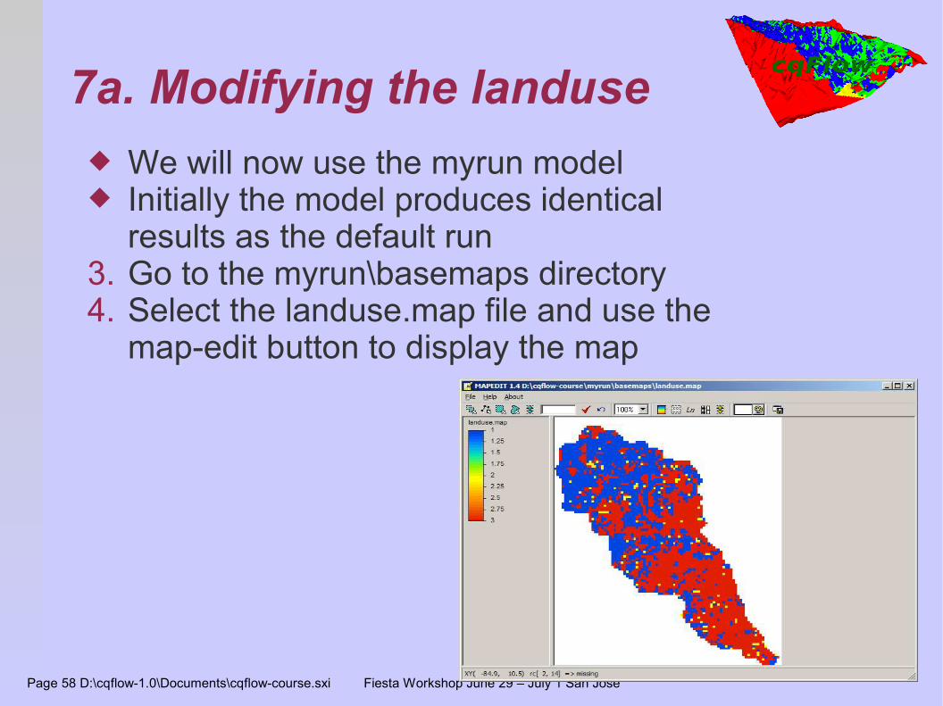
7a. Modifying the landuse We will now use the myrun model Initially the model produces identical
results as the default run3. Go to the myrun\basemaps directory4. Select the landuse.map file and use the
map-edit button to display the map
Page 59 D:\cqflow-1.0\Documents\cqflow-course.sxi Fiesta Workshop June 29 – July 1 San Jose
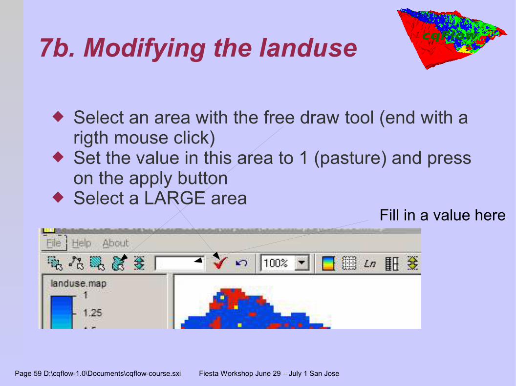
7b. Modifying the landuse
Select an area with the free draw tool (end with a rigth mouse click)
Set the value in this area to 1 (pasture) and press on the apply button
Select a LARGE areaFill in a value here
Page 60 D:\cqflow-1.0\Documents\cqflow-course.sxi Fiesta Workshop June 29 – July 1 San Jose
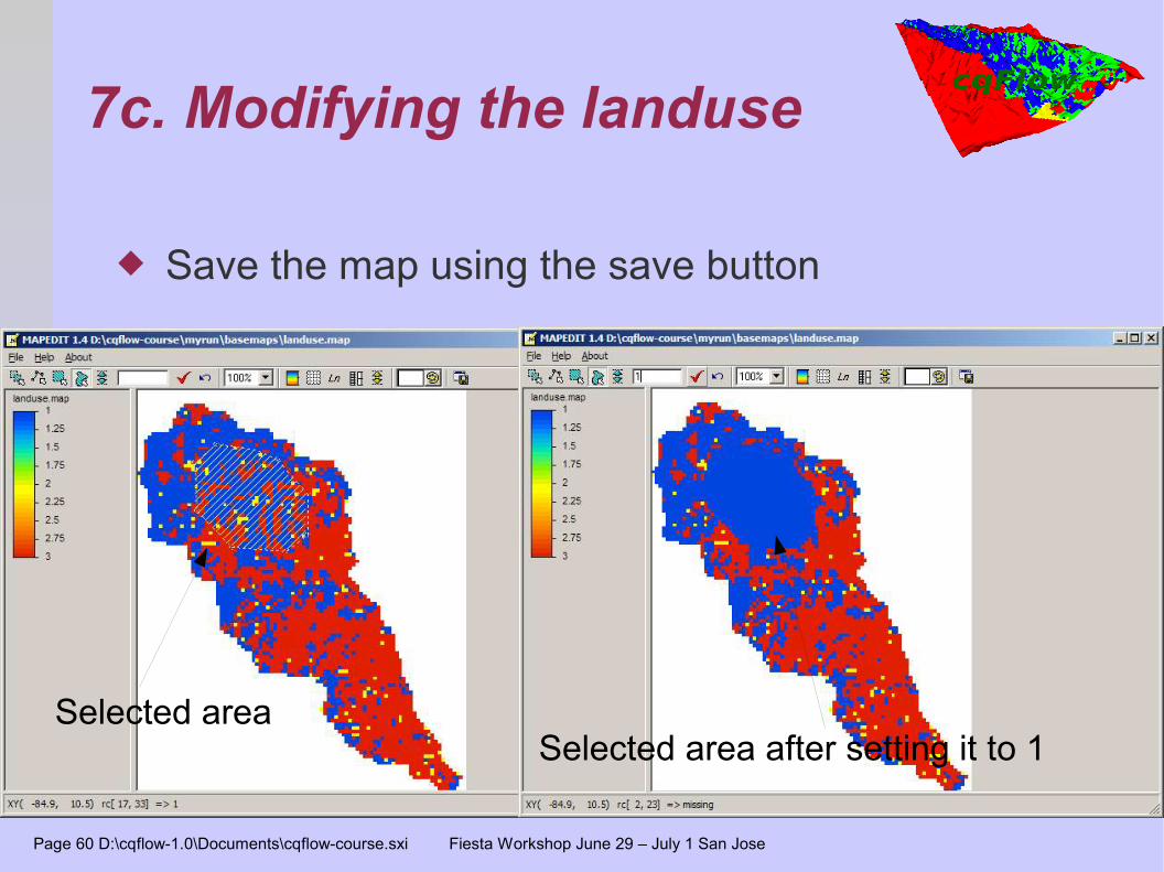
7c. Modifying the landuse
Save the map using the save button
Selected areaSelected area after setting it to 1
Page 61 D:\cqflow-1.0\Documents\cqflow-course.sxi Fiesta Workshop June 29 – July 1 San Jose
7d. Modifying the land useRe-run the model
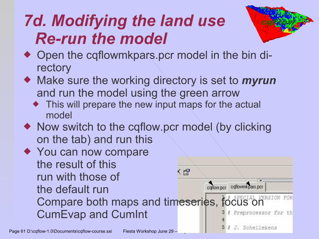
Open the cqflowmkpars.pcr model in the bin di-rectory
Make sure the working directory is set to myrun and run the model using the green arrow
This will prepare the new input maps for the actual model
Now switch to the cqflow.pcr model (by clicking on the tab) and run this
You can now comparethe result of thisrun with those ofthe default runCompare both maps and timeseries, focus on CumEvap and CumInt
Page 62 D:\cqflow-1.0\Documents\cqflow-course.sxi Fiesta Workshop June 29 – July 1 San Jose
7e. Modifying the land useComparing results
Compare timeseries by first double clicking on the .tss file in the default\outtss dir and using the “open column file” options in timeplot to open the same file from the myrun\outtss dir
Comparing maps can be done by simply opening the same map from each of the runs and showing them side by side.
Alternatively you can use the provide batch file to create a diff.map file that show the default map minus the myrun map. Make the cqflow-course dir the working dir and enter this in the command bar:diffmap CumEvap.mapYou can also use another valid map name
Display the CumEvap.mapdiff.map file by double click-ing on it. It can be found in the \cqflow-course dir
Page 63 D:\cqflow-1.0\Documents\cqflow-course.sxi Fiesta Workshop June 29 – July 1 San Jose
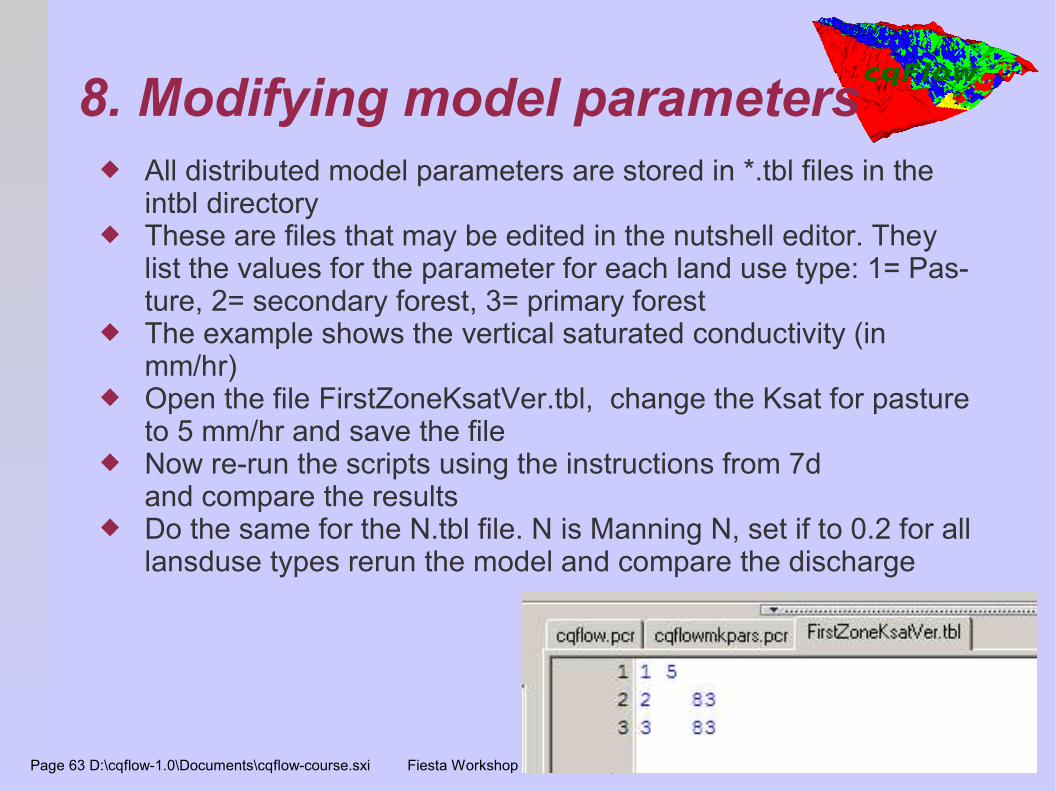
8. Modifying model parameters All distributed model parameters are stored in *.tbl files in the
intbl directory These are files that may be edited in the nutshell editor. They
list the values for the parameter for each land use type: 1= Pas-ture, 2= secondary forest, 3= primary forest
The example shows the vertical saturated conductivity (in mm/hr)
Open the file FirstZoneKsatVer.tbl, change the Ksat for pasture to 5 mm/hr and save the file
Now re-run the scripts using the instructions from 7dand compare the results
Do the same for the N.tbl file. N is Manning N, set if to 0.2 for all lansduse types rerun the model and compare the discharge

Page 64 D:\cqflow-1.0\Documents\cqflow-course.sxi Fiesta Workshop June 29 – July 1 San Jose
9. Adjusting the model
The model can easily be adjusted in the nutshell editor One simple adjustment is the save more output variables The present sstem uses the juvic gauge information. If
only normal gauges are present a regression may be used
Ratio = if (Precipitation > 0.0 then HP/Precipitation else 0.0);PrecipAngle = if (Precipitation == 0.0 then if (HP > 0.0 then 90 else 0.0) else scalar(atan(Ratio)));
#b = ln(2+0.38 * Precipitation ** 0.42);#a = 1/ln(e + 10.46 * Precipitation ** 1.24);#PrecipAngle=90- exp(4.5 - a * WindSpeed ** b);
Page 65 D:\cqflow-1.0\Documents\cqflow-course.sxi Fiesta Workshop June 29 – July 1 San Jose
Options
Discuss the cq_mkbasemaps.m script Discuss the Octave interface Adding C functions to pcraster