THE COSMIC MICROWAVE BACKGROUNDRADIATIONNobel Lecture, 8 December, 1978

byROBERT W. WILSONBell LaboratoriesHolmdel, N.J. U.S.A.

1 . I N T R O D U C T I O N

Radio Astronomy has added greatly to our understanding of the structureand dynamics of the universe. The cosmic microwave background radi-ation, considered a relic of the explosion at the beginning of the universesome 18 billion years ago, is one of the most powerful aids in determiningthese features of the universe. This paper is about the discovery of thecosmic microwave background radiation. It starts with a section on radioastronomical measuring techniques. This is followed by the history of thedetection of the background radiation, its identification, and finally by asummary of our present knowledge of its properties.

I I . RADIO ASTRONOMICAL METHODS

A radio telescope pointing at the sky receives radiation not only fromspace, but also from other sources including the ground, the earth’satmosphere, and the components of the radio telescope itself. The 20-foothorn-reflector antenna at Bell Laboratories (Fig. 1) which was used todiscover the cosmic microwave background radiation was particularly suit-ed to distinguish this weak, uniform radiation from other, much strongersources. In order to understand this measurement it is necessary to discussthe design and operation of a radio telescope, especially its two majorcomponents, the antenna and the radiometer1.

a. AntennasAn antenna collects radiation from a desired direction incident upon anarea, called its collecting area, and focuses it on a receiver. An antenna isnormally designed to maximize its response in the direction in which it ispointed and minimize its response in other directions.

The 20-foot horn-reflector shown in Fig. 1 was built by A. B. Crawfordand his associate? in 1960 to be used with an ultra low-noise communica-tions receiver for signals bounced from the Echo satellite. It consists of alarge expanding waveguide, or horn, with an off-axis section parabolicreflector at the end. The focus of the paraboloid is located at the apex ofthe horn, so that a plane wave traveling along the axis of the paraboloid isfocused into the receiver, or radiometer, at the apex of the horn. Its designemphasizes the rejection of radiation from the ground. It is easy to see

464

Fig. I The 20 foot horn-reflector which was used to discover the Cosmic Microwave Back-ground Radiation.

from the figure that in this configuration the receiver is well shielded fromthe ground by the horn.

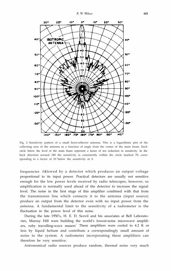
A measurement of the sensitivity of a small hornreflector antenna toradiation coming from different directions is shown in Fig. 2. The circlemarked isotropic antenna is the sensitivity of a fictitious antenna whichreceives equally from all directions. If such an isotropic lossless antennawere put in an open field, half of the sensitivity would be to radiation fromthe earth and half from the sky. In the case of the hornreflector, sensitivityin the back or ground direction is less than l/3000 of the isotropic antenna.The isotropic antenna on a perfectly radiating earth at 300 K and with acold sky at 0o K would pick up 300 K from the earth over half of itsresponse and nothing over the other half, resulting in an equivalentantenna temperature of 150 K. The horn-reflector, in contrast, would pickup less than .05 K from the ground.

This sensitivity pattern is sufficient to determine the performance of anideal, lossless antenna since such an antenna would contribute no radiationof its own. Just as a curved mirror can focus hot rays from the sun andburn a piece of paper without becoming hot itself, a radio telescope canfocus the cold sky onto a radio receiver without adding radiation of itsown.

h. RadiometersA radiometer is a device for measuring the intensity of radiation. Amicrowave radiometer consists of a filter to select a desired band of

465

Fig. 2 Sensitivity pattern of a small horn-reflector antenna. This is a logarithmic plot of thecollecting area of the antenna as a function of angle from the center of the main beam. Eachcircle below the level of the main beam represent a factor of ten reduction in sensitivity. In theback direction around 180 the sensitivity is consistently within the circle marked 70, corre-sponding to a factor of 10-7 below the sensitivity at 0.

frequencies f 11o owed by a detector which produces an output voltageproportional to its input power. Practical detectors are usually not sensitiveenough for the low power levels received by radio telescopes, however, soamplification is normally used ahead of the detector to increase the signallevel. The noise in the first stage of this amplifier combined with that fromthe transmission line which connects it to the antenna (input source)produce an output from the detector even with no input power from theantenna. A fundamental limit to the sensitivity of a radiometer is thefluctuation in the power level of this noise.

During the late 1950’s, H. E. D. Scovil and his associates at Bell Laborato-ries, Murray Hill were building the world’s lowest-noise microwave amplifi-ers, ruby travelling-wave masers3

. These amplifiers were cooled to 4.2 K orless by liquid helium and contribute a correspondingly small amount ofnoise to the system. A radiometer incorporating these amplifiers cantherefore be very sensitive.

Astronomical radio sources produce random, thermal noise very much

466 Physics 1978

like that from a hot resistor, therefore the calibration of a radiometer isusually expressed in terms of a thermal system. Instead of giving the noisepower which the radiometer receives from the antenna, we quote thetemperature of a resistor which would deliver the same noise power to theradiometer. (Radiometers often contain calibration noise sources consist-ing of a resistor at a known temperature.) This “equivalent noise tempera-ture” is proportional to received power for all except the shorter wave-length measurements, which will be discussed later.

c. ObservationsTo measure the intensity of an extraterrestrial radio source with a radiotelescope, one must distinguish the source from local noise sources - noisefrom the radiometer, noise from the ground, noise from the earth’satmosphere, and noise from the structure of the antenna itself. Thisdistinction is normally made by pointing the antenna alternately to thesource of interest and then to a background region nearby. The differencein response of the radiometer to these two regions is measured, thussubtracting out the local noise. To determine the absolute intensity of anastronomical radio source, it is necessary to calibrate the antenna andradiometer or, as usually done, to observe a calibration source of knownintensity.

I I I . PLANS FOR RADIO ASTRONOMY WITH THE 20-FOOT HORN-R E F L E C T O R

In 1963, when the 20-foot horn-reflector was no longer needed for satellitework, Arno Penzias and I started preparing it for use in radio astronomy.One might ask why we were interested in starting our radio astronomycareers at Bell Labs using an antenna with a collecting area of only 25square meters when much larger radio telescopes were available else-where. Indeed, we were delighted to have the 20-foot horn-reflector be-cause it had special features that we hoped to exploit. Its sensitivity, orcollecting area, could be accurately calculated and in addition it could bemeasured using a transmitter located less than 1 km away. With this data, itcould be used with a calibrated radiometer to make primary measure-ments of the intensities of several extraterrestrial radio sources. Thesesources could then be used as secondary standards by other observatories.In addition, we would be able to understand all sources of antenna noise,for example the amount of radiation received from the earth, so thatbackground regions could be measured absolutely. Traveling-wave maseramplifiers were available for use with the 20-foot horn-reflector, whichmeant that for large diameter sources (those subtending angles larger thanthe antenna beamwidth), this would be the world’s most sensitive radiotelescope.

My interest in the background measuring ability of the 20-foot horn-reflector resulted from my doctoral thesis work with J. G. Bolton at

R. W. Wilson 467

Caltech. We made a map of the 31 cm radiation from the Milky Way andstudied the discrete sources and the diffuse gas within it. In mapping theMilky Way we pointed the antenna to the west side of it and used theearth’s rotation to scan the antenna across it. This kept constant all thelocal noise, including radiation that the antenna picked up from the earth.I used the regions on either side of the Milky Way (where the brightnesswas constant) as the zero reference. Since we are inside the Galaxy, it isimpossible to point completely away from it. Our mapping plan wasadequate for that project, but the unknown zero level was not very satisfy-ing. Previous low frequency measurements had indicated that there is alarge, radio-emitting halo around our galaxy which I could not measure bythat technique. The 20-foot horn-reflector, however, was an ideal instru-ment for measuring this weak halo radiation at shorter wavelengths. Oneof my intentions when I came to Bell Labs was to make such a measure-ment.

In 1963, a maser at 7.35 cm wavelength3 was installed on the 20-foothorn-reflector. Before we could begin doing astronomical measurements,however, we had to do two things: 1) build a good radiometer incorporat-ing the 7.35 cm maser amplifier, and; 2) finish the accurate measurementof the collecting-area (sensitivity) of the 20-foot horn-reflector which D. C.Hogg had begun. Among our astronomical projects for 7 cm were absoluteintensity measurements of several traditional astronomical calibrationsources and a series of sweeps of the Milky Way to extend my thesis work.In the course of this work we planned to check out our capability ofmeasuring the halo radiation of our Galaxy away from the Milky Way.Existing low frequency measurements indicated that the brightness tem-perature of the halo would be less than 0.1 K at 7 cm. Thus, a backgroundmeasurement at 7 cm should produce a null result and would be a goodcheck of our measuring ability.

After completing this program of measurements at 7 cm, we planned tobuild a similar radiometer at 21 cm. At that wavelength the galactic haloshould be bright enough for detection, and we would also observe the 21cm line of neutral hydrogen atoms. In addition, we planned a number ofhydrogen-line projects including an extension of the measurements ofArno’s thesis, a search for hydrogen in clusters of galaxies.

At the time we were building the 7-cm radiometer John Bolton visited usand we related our plans and asked for his comments. He immediatelyselected the most difficult one as the most important: the 21 cm back-ground measurement. First, however, we had to complete the observationsat 7 cm.

I V . R A D I O M E T E R S Y S T E M

We wanted to make accurate measurements of antenna temperatures. Todo this we planned to use the radiometer to compare the antenna to areference source, in this case, a radiator in liquid helium. I built a switch

468

which would connect the maser amplifier either to the antenna or toArno’s helium-cooled reference noise source5 (cold load). This would allowan accurate comparison of the equivalent temperature of the antenna tothat of the cold load, since the noise from the rest of the radiometer wouldbe constant during switching. A diagram of this calibration system6 i sshown in Figure 3 and its operation is described below.

NOISE LAMP

Fig. 3 The switching and calibration system of our 7.35 cm radiometer, The reference portwas normally connected to the helium cooled reference source through a noise addingattenuator.

a. SwitchThe switch for comparing the cold load to the antenna consists of the twopolarization couplers and the polarization rotator shown in Fig. 3. Thistype of switch had been used by D. H. Ring in several radiometers atHolmdel. It had the advantage of stability, low loss, and small reflections.The circular waveguide coming from the antenna contains the two ortho-gonal modes of polarization received by the antenna. The first polarizationcoupler reflected one mode of linear polarization back to the antenna andsubstituted the signal from the cold load for it in the waveguide going tothe rotator. The second polarization coupler took one of the two modes oflinear polarization coming from the polarization rotator and coupled it tothe rectangular (single-mode) waveguide going to the maser. The polariza-tion rotator is the microwave equivalent of a half-wave plate in optics. It is a

R. W. Wilson 469

piece of circular waveguide which has been squeezed in the middle so thatthe phase shifts for waves traveling through it in its two principal planes oflinear polarization differ by 180 degrees. By mechanically rotating it, thepolarization of the signals passing through it can be rotated. Thus eitherthe antenna or cold load could be connected to the maser.

This type of switch is not inherently symmetric, but has very low loss andis stable so that its asymmetry of .05 K was accurately measured andcorrected for.

b. Reference Noise SourceA drawing of the liquid-helium cooled reference noise source is shown inFigure 4. It consists of a 122 cm piece of 90 percent-copper brass wave-guide connecting a carefully matched microwave absorber in liquid He to aroom-temperature flange at the top. Small holes allow liquid helium to fillthe bottom section of waveguide so that the absorber temperature could beknown, while a mylar window at a 30” angle keeps the liquid out of the restof the waveguide and makes a low-reflection microwave transition betweenthe two sections of waveguide. Most of the remaining parts are for thecryogenics. The gas baffles make a counter-flow heat exchanger betweenthe waveguide and the helium gas which has boiled off, greatly extendingthe time of operation on a charge of liquid helium. Twenty liters of liquidhelium cooled the cold load and provided about twenty hours of opera-tion.

Fig. 4 The Helium Cooled Reference Noise Source.

Above the level of the liquid helium, the waveguide walls were warmerthan 4.2 K. Any radiation due to the loss in this part of the waveguidewould raise the effective temperature of the noise source above 4.2 K and

470 Physics 1978

must be accounted for. To do so we monitored the temperature distribu-tion along the waveguide with a series of diode thermometers and calculat-ed the contribution of each section of the waveguide to the equivalenttemperature of the reference source. When first cooled down, the calculat-ed total temperature of the reference noise source was about 5 K, and afterseveral hours when the liquid helium level was lower, it increased to 6 K.As a check of this calibration procedure, we compared the antenna tem-perature (assumed constant) to our reference noise source during thisperiod, and found consistency to within 0.1 K.

C. Scale CalibrationA variable attenuator normally connected the cold load to the referenceport of the radiometer. This device was at room temperature so noisecould be added to the cold load port of the switch by increasing itsattenuation. It was calibrated over a range of 0.11 dB which correspondsto 7.4 K of added noise.

Also shown in Fig. 3 is a noise lamp (and its directional coupler) whichwas used as a secondary standard for our temperature scale.

d. Radiometer BackendSignals leaving the maser amplifier needed to be further amplified beforedetection so that their intensity could be measured accurately. The remain-der of our radiometer consisted of a down converter to 70 MHz followedby I. F. amplifiers, a precision variable attenuator and a diode detector.The output of the diode detector was amplified and went to a chartrecorder.

Fig. 5 Our 7.35 cm radiometer installed in the cab of the 20 foot horn-reflector.

R. W. Wilson 471

e. Equipment PerformanceOur radiometer equipment installed in the cab of the 20-foot horn-reflec-tor is shown in Fig. 5. The flange at the far right is part of the antenna androtates in elevation angle with it. It was part of a double-choke joint whichallowed the rest of the equipment to be fixed in the cab while the antennarotated. The noise contribution of the choke-joint could be measured byclamping it shut and was found to be negligible. We regularly measuredthe reflection coefficient of the major components of this system and keptit below 0.03 percent, except for the maser whose reflection could not bereduced below 1 percent. Since all ports of our waveguide system wereterminated at a low temperature, these reflections resulted in negligibleerrors.

V . P R I O R O B S E R V A T I O N SThe first horn-reflector-travelling-wave maser system had been put to-gether by DeGrasse, Hogg, Ohm, and Scovil in 19597 to demonstrate thefeasibility of a low-noise, satellite-earth station at 5.31 cm. Even thoughthey achieved the lowest total system noise temperature to date, 18.5 K,they had expected to do better. Fig. 6 shows their system with the noisetemperature they assigned to each component. As we have seen in SectionIIa ,

S I D E O R

Fig. 6 A diagram of the low noise receiver used by deGrasse, Hogg, Ohm and Scovil to showthat very low noise earth stations are possible. Each component is labeled with its contributionto the system noise.

the 2 K they assigned to antenna backlobe pickup is too high. In addition,direct measurements of the noise temperature of the maser gave a valueabout a degree colder than shown here. Thus their system was about 3 Khotter than one might expect. The component labeled Ts in Fig. 6 is theradiation of the earth’s atmosphere when their antenna was aimed straightup. It was measured by a method first reported by R. H. Dicke 8. (It isinteresting that Dicke also reports an upper limit of 20 K for the cosmicmicrowave background radiation in this paper - the first such report.) Ifthe antenna temperature is measured as a function of the angle above the

472 Physics 1978

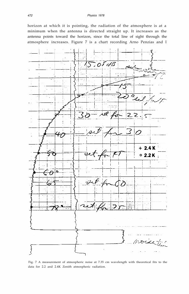
horizon at which it is pointing, the radiation of the atmosphere is at aminimum when the antenna is directed straight up. It increases as theantenna points toward the horizon, since the total line of sight through theatmosphere increases. Figure 7 is a chart recording Arno Penzias and I

Fig. 7 A measurement of atmospheric noise at 7.35 cm wavelength with theoretical fits to the

data for 2.2 and 2.4K Zenith atmospheric radiation.

R. W. Wilson 473

made with the 20-foot horn-reflector scanning from almost the Zenithdown to l(P above the horizon. The circles and crosses are the expectedchange based on a standard model of the earth’s atmosphere for 2.2 and2.4 K Zenith contribution. The fit between theory and data is obviouslygood leaving little chance that there might be an error in our value foratmospheric radiation.

Fig. 8 is taken from the paper in which E. A. Ohm 9 described thereceiver on the 20-foot horn reflector which was used to receive signalsbounced from the Echo satellite. He found that its system temperature was3.3 K higher than expected from summing the contributions of the compo-nents. As in the previous 5.3 cm work, this excess temperature was smaller

the temperature was found to vary a few degrees from day to day, butthe lowest temperature was consistently 22.2 ± 2.2”K. By realisticallyassuming that all sources were then contributing their fair share (as isalso tacitly assumed in Table II) it is possible to improve the over-allaccuracy. The actual system temperature must be in the overlap regionof the measured results and the total results of Table II, namely between20 and 21.9”K. The most likely minimum system temperature was there-fore

Fig. 8 An excerpt from E. A. Ohm’s article on the Echo receiver s h o w i n g that his systemtemperature was 3.3K higher than predicted

than the experimental errors, so not much attention was paid to it. Inorder to determine the unambiguous presence of an excess source ofradiation of about 3 K, a more accurate measurement technique was re-quired. This was achieved in the subsequent measurements by means of aswitch and reference noise source combination which communicationssystems do not have.

V I . O U R O B S E R V A T I O N S

Fig. 9 is a reproduction of the first record we have of the operation of oursystem. At the bottom is a list of diode thermometer voltages from whichwe could determine the cold load’s equivalent temperature. The recordertrace has power (or temperature) increasing to the right. The middle partof this trace is with the maser switched to the cold load with various settingsof the noise adding attenuator. A change of 0.1 dB corresponds to atemperature change of 6.6 K, so the peak-to-peak noise on the traceamounts to less than 0.2 K. At the top of the chart the maser is switched to

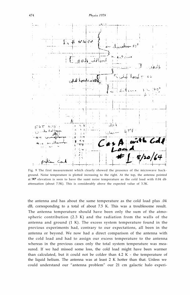
Fig. 9 The first measurement which clearly showed the presence of the microwave back-

ground. Noise temperature is plotted increasing to the right. At the top, the antenna pointedat 90” elevation is seen to have the samt noise temperature as the cold load with 0.04 dbattenuation (about 7.5K). This is considerably above the expected value of 3.3K.

the antenna and has about the same temperature as the cold load plus .04dB, corresponding to a total of about 7.5 K. This was a troublesome result.The antenna temperature should have been only the sum of the atmo-spheric contribution (2.3 K) and the radiation from the walls of theantenna and ground (1 K). The excess system temperature found in theprevious experiments had, contrary to our expectations, all been in theantenna or beyond. We now had a direct comparison of the antenna withthe cold load and had to assign our excess temperature to the antennawhereas in the previous cases only the total system temperature was mea-sured. If we had missed some loss, the cold load might have been warmerthan calculated, but it could not be colder than 4.2 K - the temperature ofthe liquid helium. The antenna was at least 2 K hotter than that. Unless wecould understand our “antenna problem” our 21 cm galactic halo experi-

R. W. Wilson 475

ment would not be possible. We considered a number of possible reasonsfor this excess and, where warranted, tested for them. These were:a. At that time some radio astronomers thought that the microwave ab-

sorption of the earth’s atmosphere was about twice the value we wereusing - in other words the “sky temperature” of Figs. 6 and 8 was about5 K instead of 2.5 K. We knew from our measurement of sky tempera-ture such as shown in Fig. 7 that this could not be the case.

b. We considered the possibility of man-made noise being picked up byour antenna. However, when we pointed our antenna to New YorkCity, or to any other direction on the horizon, the antenna temperaturenever went significantly above the thermal temperature of the earth.

c. We considered radiation from our galaxy. Our measurements of theemission from the plane of the Milky Way were a reasonable fit to theintensities expected from extrapolations of low-frequency measure-ments. Similar extrapolations for the coldest part of the sky (away fromthe Milky Way) predicted about .02 K at our wavelength. Furthermore,any galactic contribution should also vary with position and we sawchanges only near the Milky Way, consistent with the measurements atlower frequencies.

d. We ruled out discrete extraterrestrial radio sources as the source of ourradiation as they have spectra similar to that of the Galaxy. The sameextrapolation from low frequency measurements applies to them. Thestrongest discrete source in the sky had a maximum antenna tempera-ture of 7 K.

Thus we seemed to be left with the antenna as the source of our extranoise. We calculated a contribution of 0.9 K from its resistive loss usingstandard waveguide theory. The most lossy part of the antenna was itssmall diameter throat, which was made of electroformed copper. We hadmeasured similar waveguides in the lab and corrected the loss calculationsfor the imperfect surface conditions we had found in those waveguides.The remainder of the antenna was made of riveted aluminum sheets, andalthough we did not expect any trouble there, we had no way to evaluatethe loss in the riveted joints. A pair of pigeons was roosting up in the smallpart of the horn where it enters the warm cab. They had covered the insidewith a white material familiar to all city dwellers. We evicted the pigeonsand cleaned up their mess, but obtained only a small reduction in antennatemperature.

For some time we lived with the antenna temperature problem andconcentrated on measurements in which it was not critical. Dave Hogg andI had made a very accurate measurement of the antenna’s gain10, andArno and I wanted to complete our absolute flux measurements beforedisturbing the antenna further.

In the spring of 1965 with our flux measurements finished5, we thor-oughly cleaned out the 20-foot horn-reflector and put aluminum tape overthe riveted joints. This resulted in only a minor reduction in antennatemperature. We also took apart the throat section of the antenna, andchecked it, but found it to be in order.

476 Physics 1978

By this time almost a year had passed. Since the excess antenna tempera-ture had not changed during this time, we could rule out two additionalsources: 1) Any source in the solar system should have gone through alarge change in angle and we should have seen a change in antennatemperature. 2) In 1962, a high-altitude nuclear explosion had filled upthe Van Allen belts with ionized particles. Since they were at a largedistance from the surface of the earth, any radiation from them would notshow the same elevation-angle dependence as the atmosphere and wemight not have identified it. But after a year, any radiation from thissource should have reduced considerably.

V I I . I D E N T I F I C A T I O N

The sequence of events which led to the unravelling of our mystery beganone day when Arno was talking to Bernard Burke of M.I.T. about othermatters and mentioned our unexplained noise. Bernie recalled hearingabout theoretical work of P. J. E. Peebles in R. H. Dicke’s group inPrinceton on radiation in the universe. Arno called Dicke who sent a copyof Peebles’ preprint. The Princeton group was investigating the implica-tions of an oscillating universe with an extremely hot condensed phase.This hot bounce was necessary to destroy the heavy elements from theprevious cycle so each cycle could start fresh. Although this was not a newidea” Dicke had the important idea that if the radiation from this hotphase were large enough, it would be observable. In the preprint, Peebles,following Dicke’s suggestion calculated that the universe should be filledwith a relic blackbody radiation at a minimum temperature of 10 K.Peebles was aware of Hogg and Semplak’s (1961)12 measurement of atmo-spheric radiation at 6 cm using the system of DeGrasse et al., and conclud-ed that the present radiation temperature of the universe must be less thantheir system temperature of 15 K. He also said that Dicke, Roll, andWilkinson were setting up an experiment to measure it.

Shortly after sending the preprint, Dicke and his coworkers visited us inorder to discuss our measurements and see our equipment. They werequickly convinced of the accuracy of our measurements. We agreed to aside-by-side publication of two letters in the Astrophysical Journal - a letter onthe theory from Princeton 13 and one on our measurement of excess anten-na temperature from Bel l Laborator ies 14. Arno and I were careful toexclude any discussion of the cosmological theory of the origin of back-ground radiation from our letter because we had not been involved in anyof that work. We thought, furthermore, that our measurement was inde-pendent of the theory and might outlive it. We were pleased that themysterious noise appearing in our antenna had an explanation of anykind, especially one with such significant cosmological implications. Ourmood, however, remained one of cautious optimism for some time.

R.W. Wilson 477

V I I I . R E S U L T S

While preparing our letter for publication we made one final check on theantenna to make sure we were not picking up a uniform 3 K from earth.We measured its response to radiation from the earth by using a transmit-ter located in various places on the ground. The transmitter artificiallyincreased the ground’s brightness at the wavelength of our receiver to alevel high enough for the backlobe response of the antenna to be measur-able. Although not a perfect measure of the structure of the backlobes ofan antenna, it was a good enough method of determining their averagelevel. The backlobe level we found in this test was as low as we hadexpected and indicated a negligible contribution to the antenna tempera-ture from the earth.

The right-hand column of Fig. 10 shows the final results of our measure-ment. The numbers on the left were obtained later in 1965 with a newthroat on the 20-foot horn-reflector. From the total antenna temperaturewe subtracted the known sources with a result of 3.4 ± 1 K. Since the errorsin this measurement are not statistical, we have summed the maximumerror from each source. The maximum measurement error of 1 K wasconsiderably smaller than the measured value, giving us confidence in thereality of the result. We stated in the original paper that “This excesstemperature is, within the limits of our observations, isotropic, unpolar-ized, and free of seasonal variations”. Although not stated explicitly, ourlimits on an isotropy and polarization were not affected by most of theerrors listed in Fig. 10 and were about 10 percent or 0.3 K.

New Throat Old Throat

Fig. 10 Results of our 3965 measurements of the microwave background. “Old Throat” and“New Throat” refer to the original and a replacement throat section for the 20 foot horn-reflector.

478 Physics 1978

At that time the limit we could place on the shape of the spectrum of thebackground radiation was obtained by comparing our value of 3.5 K with a74 cm survey of the northern sky done at Cambridge by Pauliny-Toth andShakeshaft, 196215. The minimum temperature on their map was 16 K.Thus the spectrum was no steeper than λ 0.7 over a range of wavelengthsthat varied by a factor of 10. This clearly ruled out any type of radio sourceknown at that time, as they all had spectra with variation in the range λ 2.0

to λ 3.0. The previous Bell Laboratories measurement at 6 cm ruled out aspectrum which rose rapidly toward shorter wavelengths.

I X . C O N F I R M A T I O N

After our meeting, the Princeton experimental group returned to com-plete their apparatus and make their measurement with the expectationthat the background temperature would be about 3 K.

The first confirmation of the microwave cosmic background that weknew of, however, came from a totally different, indirect measurement.This measurement had, in fact, been made thirty years earlier by Adamsand Dunhan16-21. Adams and Dunhan had discovered several faint opticalinterstellar absorption lines which were later identified with the moleculesC H , C H+, and CN. In the case of CN, in addition to the ground state,absorption was seen from the first rotationally excited state. McKellar22

using Adams’ data on the populations of these two states calculated thatthe excitation temperature of CN was 2.3 K. This rotational transitionoccurs at 2.64 mm wavelength, near the peak of a 3 K black body spec-trum. Shortly after the discovery of the background radiation, G. B.Field 23, I. S. Shklovsky24, and P. Thaddeus25 (following a suggestion by N.J. Woolf), independently realized that the CN is in equilibrium with thebackground radiation. (There is no other significant source of excitationwhere these molecules are located). In addition to confirming that thebackground was not zero, this idea immediately confirmed that the spec-trum of the background radiation was close to that of a blackbody sourcefor wavelengths larger than the peak. It also gave a hint that at shortwavelengths the intensity was departing from the 1 /A* dependence expect-ed in the long wavelength (Raleigh-Jeans) region of the spectrum andfollowing the true blackbody (Plank) distribution. In 1966, Field andHitchcock 23 reported new measurements using Herbig’s plates of 4 Opha n d 5 Per obtaining 3.22 ± 0.15 K and 3.0 ± 0.6 K for the excitationtemperature. Thaddeus and Clauser 25 also obtained new plates and mea-sured 3.75 ± 0.5 K in c Oph. Both groups argued that the main source ofexcitation in CN is the background radiation. This type of observation,taken alone, is most convincing as an upper limit, since it is easier toimagine additional sources of excitation than refrigeration.

In December 1965 Roll and Wilkinson26 completed their measurementof 3.0 ± 0.5 K at 3.2 cm, the first confirming microwave measurement.This was followed shortly by Howell and Shakeshaft's27 value of 2.8 ± 0.6

R. W. Wilson 479

K at 20.7 cm22 and then by our measurement of 3.2 K ± 1 K at 21.1 cm 28.(Half of the difference between these two results comes from a differencein the corrections used for the galactic halo and integrated discretesources.) By mid 1966 the intensity of the microwave background radi-ation had been shown to be close to 3 K between 21 cm and 2.6 mm, almosttwo orders of magnitude in wavelength.

X. EARLIER THEORY

I have ment ioned that the f i rs t exper imental evidence for cosmicmicrowave background radiation was obtained (but unrecognized) longbefore 1965. We soon learned that the theoretical prediction of it had beenmade at least sixteen years before our detection. George Gamow had madecalculations of the conditions in the early universe in an attempt to under-stand Galaxy formation29. Although these calculations were not strictlycorrect, he understood that the early stages of the universe had to be veryhot in order to avoid combining all of the hydrogen into heavier elements.Furthermore, Gamow and his collaborators calculated that the density ofradiation in the hot early universe was much higher than the density ofmatter. In this early work the present remnants of this radiation were notconsidered. However in 1949, Alpher and Herman30 followed the evolu-tion of the temperature of the hot radiation in the early universe up to thepresent epoch and predicted a value of 5 K. They noted that the presentdensity of radiation was not well known experimentally. In 1953 Alpher,Follin, and Herman31 reported what has been called the first thoroughlymodern analysis of the early history of the universe, but failed to recalcu-late or mention the present radiation temperature of the universe.

In 1964, Doroshkevich and Novikov 32 33 had a lso ca lculated the re l ic,radiation and realized that it would have a blackbody spectrum. Theyquoted E. A. Ohm’s article on the Echo receiver, but misunderstood it andconcluded that the present radiation temperature of the universe is nearzero.

A more complete discussion of these early calculations is given in Arno’slecture. 34

XI. ISOTROPY

In assigning a single temperature to the radiation in space, these theoriesassume that it will be the same in all directions. According to contemporarytheory, the last scattering of the cosmic microwave background radiationoccurred when the universe was a million years old, just before the elec-trons and nucleii combined to form neutral atoms (“recombination”).Theisotropy of the background radiation thus measures the isotropy of theuniverse at that time and the isotropy of its expansion since then. Prior torecombination, radiation dominated the ‘universe and the Jeans mass, ormass of the smallest gravitationally stable clumps was larger than a clusterof Galaxies. It is only in the period following recombination that Galaxiescould have formed.

480

ANGLE BETWEEN INSTRUMENT DIRECTION AND SITEOF MAXIMUM TEMPERATURE (DEGREES)

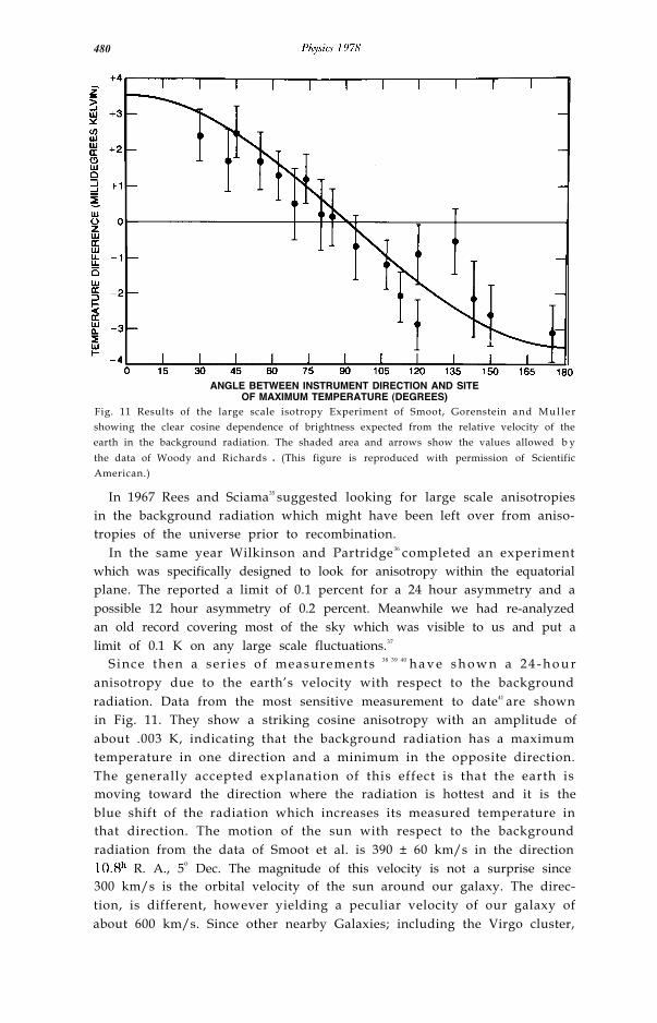
Fig. 11 Results of the large scale isotropy Experiment of Smoot, Gorenstein and M u l l e rshowing the clear cosine dependence of brightness expected from the relative velocity of theearth in the background radiation. The shaded area and arrows show the values allowed b ythe data of Woody and Richards . (This figure is reproduced with permission of ScientificAmerican.)

In 1967 Rees and Sciama35 suggested looking for large scale anisotropiesin the background radiation which might have been left over from aniso-tropies of the universe prior to recombination.

In the same year Wilkinson and Partridge36 completed an experimentwhich was specifically designed to look for anisotropy within the equatorialplane. The reported a limit of 0.1 percent for a 24 hour asymmetry and apossible 12 hour asymmetry of 0.2 percent. Meanwhile we had re-analyzedan old record covering most of the sky which was visible to us and put alimit of 0.1 K on any large scale fluctuations.37

S ince then a ser ies of measurements 38 39 40 h a v e s h o w n a 2 4 - h o u ranisotropy due to the earth’s velocity with respect to the backgroundradiation. Data from the most sensitive measurement to date41 are shownin Fig. 11. They show a striking cosine anisotropy with an amplitude ofabout .003 K, indicating that the background radiation has a maximumtemperature in one direction and a minimum in the opposite direction.The generally accepted explanation of this effect is that the earth ismoving toward the direction where the radiation is hottest and it is theblue shift of the radiation which increases its measured temperature inthat direction. The motion of the sun with respect to the backgroundradiation from the data of Smoot et al. is 390 ± 60 km/s in the direction10.Sh R. A., 5o Dec. The magnitude of this velocity is not a surprise since300 km/s is the orbital velocity of the sun around our galaxy. The direc-tion, is different, however yielding a peculiar velocity of our galaxy ofabout 600 km/s. Since other nearby Galaxies; including the Virgo cluster,

R. W Wilson 481

have a small velocity with respect to our Galaxy, they have a similar velocitywith respect to the matter which last scattered the background radiation.After subtracting the 24-hour anisotropy, one can search the data for morecomplicated anisotropies to put observational limits on such things asrotation of the universe41. Within the noise of .001 K, these anisotropiesare all zero.

To date, no fine-scale anisotropy has been found. Several early investiga-tions were carried out to discredit discrete source models of the back-ground radiation. In the most sensitive experiment to date, Boynton andPartridge 42 report a relative intensity variation of less than 3.7 x 10-3 in an80” Arc beam. A discrete source model would require orders of magnitudemore sources than the known number of Galaxies to show this degree ofsmoothness.

It has also been suggested by Sunyaev and Zel’dovich43 that there will bea reduction of the intensity of the background radiation from the directionof clusters of galaxies due to inverse Compton scattering by the electronsin the intergalactic gas. This effect which has been found by Birkinshawand Gull 44, provides a measure of the intergalactic gas density in theclusters and may give an alternate measurement of Hubble’s constant.

XII . SPECTRUM

Since 1966, a large number of measurements of the intensity of thebackground radiation have been made at wavelengths from 74 cm to 0.5mm. Measurements have been made from the ground, mountain tops,

482 Physics 1978

airplanes, balloons, and rockets. In addition, the optical measurements ofthe interstellar molecules have been repeated and we have observed theirmillimeter-line radiation directly to establish the equilibrium of the excita-tion of their levels with the background radiation45. Fig. 12 is a plot of mostof these measurements46. An early set of measurements from Princetoncovered the range 3.2 to .33 cm showing tight consistency with a 2.7 Kblack body 47-50 . A series of rocket and balloon measurements in themillimeter and submillimeter part of the spectrum have converged onabout 3 K. The data of Robson, et al. 51 and Woody and Richards52 extendto 0.8 mm, well beyond the spectral peak. The most recent experiment,that of D. Woody and P. Richards, gives a close fit to a 3.0 K spectrum outto 0.8 mm wavelength with upper limits at atmospheric windows out to 0.4mm. This establishes that the background radiation has a blackbody spec-trum which would be quite hard to reproduce with any other type ofcosmic source. The source must have been optically thick and thereforemust have existed earlier than any of the other sources, which can beobserved.

The spectral data are now almost accurate enough for one to test forsystematic deviations from a single-temperature blackbody spectrumwhich could be caused by minor deviations from the simplest cosmology.Danese and DeZotti53 report that except for the data of Woody andRichards, the spectral data of Fig. 12 do not show any statistically signifi-cant deviation of this type.

XIII . CONCLUSION

Cosmology is a science which has only a few observable facts to work with.The discovery of the cosmic microwave background radiation added one- the present radiation temperature of the universe. This, however, was asignificant increase in our knowledge since it requires a cosmology with asource for the radiation at an early epoch and is a new probe of that epoch.More sensitive measurements of the background radiation in the futurewill allow us to discover additional facts about the universe.

XIV. ACKNOWLEDGMENTSThe work which I have described was done with Arno A. Penzias. In ourfifteen years of partnership he has been a constant source of help andencouragement. I wish to thank W. D. Langer and Elizabeth Wilson forcarefully reading the manuscript and suggesting changes.

REFERENCES1. A more complete discussion of radio telescope antennas and receivers may be found in

several text books. Chapters 6 and 7 of J. D. Kraus “Radio Astronomy”, 1966, McGraw-Hill are good introductions to the subjects.

2. Crawford, A. B. Hogg, D. C. and Hunt, L. E. 1961, Bell System Tech. J., 40, 1095.

R. W. Wilson 483

3. DeGrasse, R. W. Schultr-DuBois, E. 0. and Scovil, H. E. D. BSTJ 38, 30.5.4. Tabor, W. J. and Sibilia, J. 1‘. 1963, Bell System Tech. J., 42, 1863.5. Penzias, A. A. 1965, Rev. Sci. Instr., 36. 68.6. Penzias, A. A. and Wilson, R. W. 1965 Astrophysical Journal 142. 1149.7. DeGrasse, R. W. Hogg, D. C. Ohm, E. A. and Scovil, H. E. D. 1950, Proceedings of the

National Electronics Conference. 15, 370.8. Dicke. R. Beringer R. Kyhl, R. L. and Vane, A. V. Phys. Rev. 70, 340 (1046).9, Ohm, E. A. 1961 BSTJ, 40, 1065.

10. Hogg, D. C. and Wilson, R. W. Bell system Tech J., 44, 1019.11. c.f. F. Hoyle and R. J. Taylor 1964. Nature 203, 1108. A less explicit discussion of the

same notion occurs in [29].12. Hogg, D. C. and Semplak, R. A. 1961, Bell System Technical Journal. 40, 1331 .13. Dicke, R. H. Peebles, P. J. E. Roll, P. G. and Wilkinson, D. T. 1965, Ap. J., 142. 4 14.14. Penzias, A. A. and Wilson R. W. 1965, Ap. J.. 142, 420.15. Pauliny-Toth, I. I. K. and Shakeshaft, J. R. 1962, M. N. RAS.. 124, 61.16. Adams, W. S. 1941, Ap. J. 93, 11.17. Adams, W. S. 1943, Ap. J., 97, 105.18. Dunham, T. Jr. 1937, PASP, 49, 26.19. Dunham, T. Jr. 1939, Proc. Am. Phil. Soc., 81, 277.20. Dunham, T. Jr. 1941, Publ. Am. Astron. Soc., 10, 123.21. Dunham, T. Jr. and W. S. Adams 1937, Publ. Am. Astron. Soc., 9, 5.22. McKellar, A. 1941, Publ. Dominion Astrophysical Observatory Victoria B. C. 7, 251.23. G. B. Field, G. H. Herbig and J. L. Hitchcock, talk at the American Astronomical Society

Meeting, 22-29 December 1965, Astronomical Journal 1966, 71. 161; G. B. Field and J .I,. Hitchcock, 1966, Phys. Rev. Lett. 16, 8 17.

24. Shklovsky, I. S. 1966, Astron. Circular No. 364, Acad. Sci. USSR.25. Thaddeus, P. and Clauser, J. F. 1966, Phys. Rev. Lett. 16, 8 19.26. Roll, P. G. and Wilkinson, D. T. 1966, Physical Review Letters, 16, 405.27. Howell, T. F. and Shakeshaft, J. R. 1966, Nature 210, 138.28. Penzias, A. A. and Wilson R. W. 1967, Astron. J. 72, 315.29. Gamow, G. 1948, Nature I62 680.30. Alpher, R. .4. and Herman, R. C. 1949, Phys. Rev., 75, 1089.31. Alpher, R. A. Follin, J. W. and Herman, R. C. 1953, Phys. Rev., 92, 1347.32. Doroshkevich, A. G. and Novikov. I. D. 1964 Dokl. Akad. Navk. SSR 154, 809.33. Doroshkevich, A. G. and Novikov, I. D. 1964 Sov. Phys. Dokl. 9, 111 .34. Penzias, A. A. The Origin of the Elements, Nobel Prize lecture 1978.3.5. Rees, M. J. and Sciama, D. W. 1967, Nature, 213, 374.36. Partridge, R. B. and Wilkinson, D. T. 1967, Nature, 215, 7 19.37. Wilson, R. W. and Penzias, A. A. 1967, Science 156, 1100.38. Conklin, E. K. 1969, Nature, 222, 97 I.39. Henry, P. S. 1971, Nature, 231, 516.40. Corey, B. E. and Wilkinson, D. T. 1976, Bull. Astron. Astrophys. Soc., 8, 351.41. Smoot, G. F. Gorenstein, M. V. and Muller, R. A. 1977, Phys. Rev. Lett., 39, 898.42. Boynton, P. E. and Partridge, R. B. 1973, Ap. J., 181, 243.43. Sunyaev, R. A. and Zel’dovich, Ya B 1972, Comments Astrophys. Space Phys., 4, 173.44. Birkinshaw, M. and Gull, S. F. 1978, Nature275 40.45. Penzias, A. A. Jefferts, K. B. and Wilson, R. W’. 1972, Phys. Rev. Letters, 28, 772.46. The data in Fig. 11 are all referenced by Danese and Dezotti 45 except for the 13 cm

measurement of T. Otoshi 1975, IEEE Trans on Instrumentation and Meas. 24 174. Ihave used the millimeter measurements of Woody and Richards 48 and left off those ofRobson et al47 to avoid confusion.

47. Wilkinson, D. J. 1967, Phys. Rev. Letters. 19, 1195.48. Stokes, R. A. Partridge, R. B. and Wilkinson, D. J. 1967. Phys. Rev. Letters, 19, 1199.49. Boynton, P. E. Stokes, R. A. and Wilkinson, D. J. 1968, Phys. Rev. Letters, 21, 462.50. Boynton, P. E. and Stokes, R. A. 1974, Nature, 247, 528.51. Robson, E. I. Vickers, D. G. Huizinga, J. S. Beckman.J. E. and Clegg, P. E. 1974, Nature

251, 591.52. Woody, D. P. and Richards, P. L. Private communication.53. Danese, L. and DeZotti, G. 1978, Astron. and Astrophys.. 68, 157.