The Contribution of Biomass to Emissions Mitigation under a

Global Climate PolicyNiven Winchester and John M. Reilly

Report No. 273January 2015

The MIT Joint Program on the Science and Policy of Global Change combines cutting-edge scientific research with independent policy analysis to provide a solid foundation for the public and private decisions needed to mitigate and adapt to unavoidable global environmental changes. Being data-driven, the Program uses extensive Earth system and economic data and models to produce quantitative analysis and predictions of the risks of climate change and the challenges of limiting human influence on the environment—essential knowledge for the international dialogue toward a global response to climate change.

To this end, the Program brings together an interdisciplinary group from two established MIT research centers: the Center for Global Change Science (CGCS) and the Center for Energy and Environmental Policy Research (CEEPR). These two centers—along with collaborators from the Marine Biology Laboratory (MBL) at Woods Hole and short- and long-term visitors—provide the united vision needed to solve global challenges.

At the heart of much of the Program’s work lies MIT’s Integrated Global System Model. Through this integrated model, the Program seeks to: discover new interactions among natural and human climate system components; objectively assess uncertainty in economic and climate projections; critically and quantitatively analyze environmental management and policy proposals; understand complex connections among the many forces that will shape our future; and improve methods to model, monitor and verify greenhouse gas emissions and climatic impacts.

This reprint is one of a series intended to communicate research results and improve public understanding of global environment and energy challenges, thereby contributing to informed debate about climate change and the economic and social implications of policy alternatives.

Ronald G. Prinn and John M. Reilly, Program Co-Directors

For more information, contact the Program office: MIT Joint Program on the Science and Policy of Global Change

Postal Address: Massachusetts Institute of Technology 77 Massachusetts Avenue, E19-411 Cambridge, MA 02139 (USA)

Location: Building E19, Room 411 400 Main Street, Cambridge

Access: Tel: (617) 253-7492 Fax: (617) 253-9845 Email: globalchange@mit.edu Website: http://globalchange.mit.edu/

1

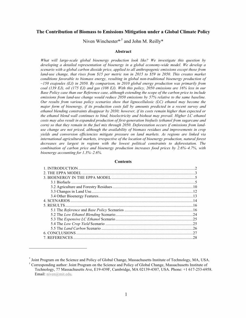
The Contribution of Biomass to Emissions Mitigation under a Global Climate Policy

Niven Winchester*,† and John M. Reilly*

Abstract

What will large-scale global bioenergy production look like? We investigate this question by developing a detailed representation of bioenergy in a global economy-wide model. We develop a scenario with a global carbon dioxide price, applied to all anthropogenic emissions except those from land-use change, that rises from $15 per metric ton in 2015 to $59 in 2050. This creates market conditions favorable to biomass energy, resulting in global non-traditional bioenergy production of ~150 exajoules (EJ) in 2050. By comparison, in 2010 global energy production was primarily from coal (139 EJ), oil (175 EJ) and gas (108 EJ). With this policy, 2050 emissions are 16% less in our Base Policy case than our Reference case, although extending the scope of the carbon price to include emissions from land-use change would reduce 2050 emissions by 57% relative to the same baseline. Our results from various policy scenarios show that lignocellulosic (LC) ethanol may become the major form of bioenergy, if its production costs fall by amounts predicted in a recent survey and ethanol blending constraints disappear by 2030; however, if its costs remain higher than expected or the ethanol blend wall continues to bind, bioelectricity and bioheat may prevail. Higher LC ethanol costs may also result in expanded production of first-generation biofuels (ethanol from sugarcane and corn) so that they remain in the fuel mix through 2050. Deforestation occurs if emissions from land-use change are not priced, although the availability of biomass residues and improvements in crop yields and conversion efficiencies mitigate pressure on land markets. As regions are linked via international agricultural markets, irrespective of the location of bioenergy production, natural forest decreases are largest in regions with the lowest political constraints to deforestation. The combination of carbon price and bioenergy production increases food prices by 2.6%–4.7%, with bioenergy accounting for 1.3%–2.6%.

Contents 1. INTRODUCTION .................................................................................................................... 22. THE EPPA MODEL ................................................................................................................ 33. BIOENERGY IN THE EPPA MODEL ................................................................................... 5

3.1 Biofuels ........................................................................................................................... 5  3.2 Agriculture and Forestry Residues ................................................................................ 10  3.3 Changes in Land Use ..................................................................................................... 12  3.4 Other Bioenergy Features .............................................................................................. 13  

4. SCENARIOS .......................................................................................................................... 145. RESULTS ............................................................................................................................... 16

5.1 The Reference and Base Policy Scenarios .................................................................... 16  5.2 The Low Ethanol Blending Scenario ............................................................................. 24  5.3 The Expensive LC Ethanol Scenario ............................................................................. 25  5.4 The Low Crop Yield Scenario ....................................................................................... 25  5.5 The Land Carbon Scenario ........................................................................................... 26  

6. CONCLUSIONS .................................................................................................................... 277. REFERENCES ....................................................................................................................... 28

* Joint Program on the Science and Policy of Global Change, Massachusetts Institute of Technology, MA, USA.† Corresponding author: Joint Program on the Science and Policy of Global Change, Massachusetts Institute of

Technology, 77 Massachusetts Ave, E19-439F, Cambridge, MA 02139-4307, USA. Phone: +1 617-253-6958. Email: niven@mit.edu.

2

1. INTRODUCTION

Policies in Europe and in the United States have created an expanding market for biofuels, on top of the successful sugar-based biofuels development in Brazil. These biofuels mandates are part of a suite of current or proposed policies to address energy security, climate change and sustainability issues. Greenhouse gas (GHG) emissions abatement through biomass energy production raises a number of questions, such as:

• Given the multiple pathways with which biomass can be used to produce energy, what bioenergy technologies will prevail?

• What are the GHG implications of expanding bioenergy when accounting for the potential need to expand cropland or apply nitrogen fertilizer?

• Where will bioenergy feedstocks be grown? • How will large-scale bioenergy production affect food prices? • Will land-use limitation policy, intended to protect forested land with large carbon

stocks, also limit bioenergy expansion by increasing land prices? Although a large body of literature on bioenergy has emerged, most studies consider forced

targets with specific and limited fuel conversion pathways, rather than considering the optimal use of biomass feedstocks and conversion technologies in abating emissions while accounting for economic and physical constraints. For example, Rahdar et al. (2014) examined competition for biomass between bioelectricity and biofuels in the US under a renewable electricity standard and renewable fuel mandates. Wise et al. (2014) evaluated the impact of existing, moderate and high (up to 25% of transportation fuel) global biofuel mandates using the Global Change Assessment Model. Melillo et al. (2009) and Reilly et al. (2012) considered large-scale biofuel development with a simplified second-generation biofuel production technology; however, this provided no insight into the potential competition among first- and second-generation biofuel pathways or uses of biomass for fuels, power generation, and industrial heat.

We contribute to the existing literature by evaluating the role of bioenergy under a global carbon price, where the level and composition of bioenergy production is determined on an economic basis, and identifying numerous crops and pathways through which biomass could supply global energy needs. Our analysis employs a global model of economic activity and energy production that is augmented to represent bioenergy in detail. Bioenergy technologies represented include (1) seven first-generation biofuel crops and conversion technologies; (2) an energy grass and a woody crop; (3) agricultural and forestry residues; (4) two lignocellulosic biofuel conversion technologies, which can operate with and without carbon capture and storage (CCS); (5) an ethanol-to-diesel upgrading process; (6) electricity from biomass, with and without CCS; and (7) heat from biomass for use in industrial sectors. The model also includes explicit representation of bioenergy co-products (e.g. distillers’ dry grains and surplus electricity), international trade in biofuels and pelletized woody feedstocks, land-use change with explicit representation of conversion costs and political constraints, limits on the blending of ethanol with

3

gasoline, endogenous changes in land and other production costs, and price-induced changes in energy efficiency and alternative vehicle technologies. Compared to previous investigations, our approach has far more detail on the conversion pathways and potential role of biomass energy.

This paper has five further sections. Section 2 outlines the core economy-wide model used for our analysis. Section 3 sets out the representation of bioenergy in the model. The scenarios implemented are outlined in Section 4. Section 5 presents and discusses results. Section 6 concludes.

2. THE EPPA MODEL

Our analysis builds on version 5 of the Economic Projection and Policy Analysis (EPPA) model, a recursive-dynamic, multi-region computable general equilibrium global model of economic activity, energy production and GHG emissions (Paltsev et al., 2005), as augmented to consider land use change (Gurgel et al., 2007, 2011). We further extend the model to include a detailed representation of bioenergy production and use. Version 5 of the EPPA model is solved through time in five-year increments and is calibrated using economic data from Version 7 of the Global Trade Analysis Project (GTAP) database (Narayanan & Walmsley, 2008), population forecasts from the United Nations Population Division (UN, 2011), and energy data from the International Energy Agency (IEA, 2004). Regional economic growth through 2015 is calibrated to International Monetary Fund (IMF) data (IMF, 2013). The model is coded using the General Algebraic Modeling System (GAMS) and the Mathematical Programming System for General Equilibrium analysis (MPSGE) modeling language (Rutherford, 1995).

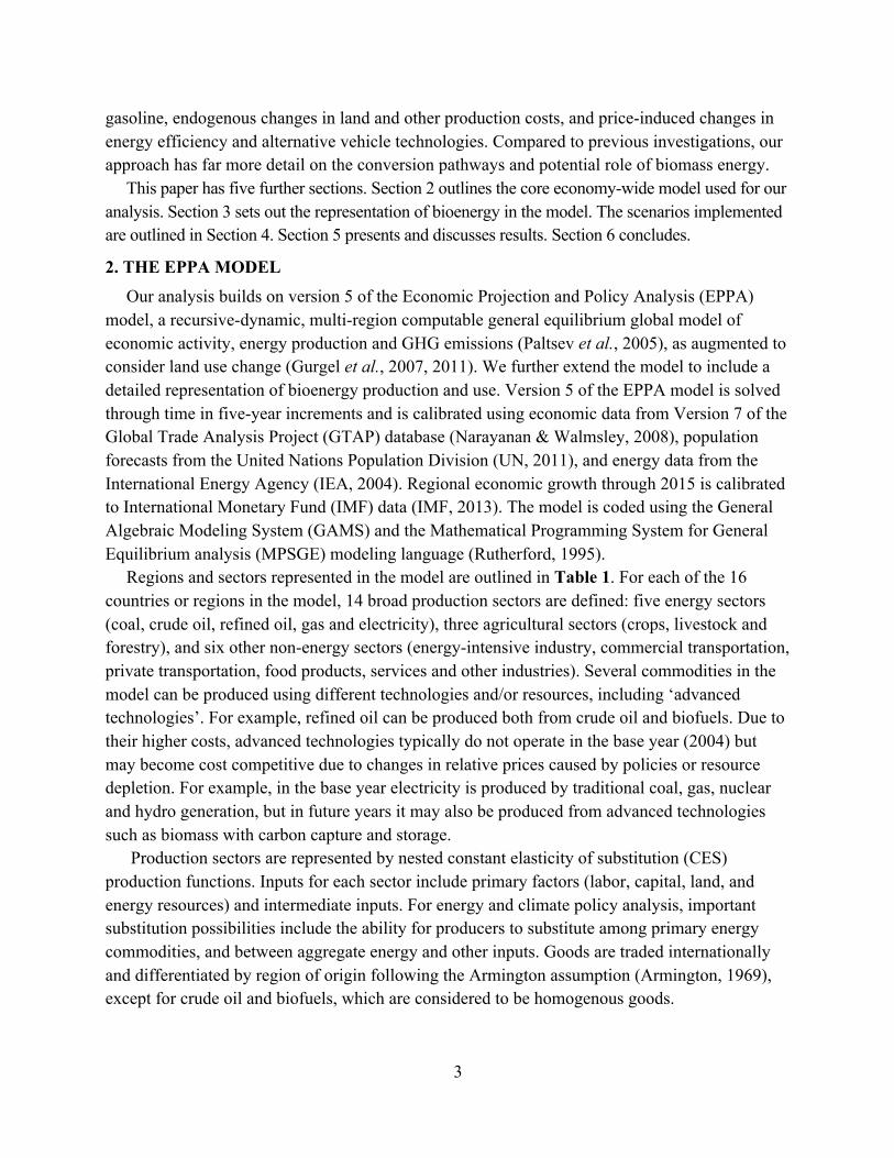
Regions and sectors represented in the model are outlined in Table 1. For each of the 16 countries or regions in the model, 14 broad production sectors are defined: five energy sectors (coal, crude oil, refined oil, gas and electricity), three agricultural sectors (crops, livestock and forestry), and six other non-energy sectors (energy-intensive industry, commercial transportation, private transportation, food products, services and other industries). Several commodities in the model can be produced using different technologies and/or resources, including ‘advanced technologies’. For example, refined oil can be produced both from crude oil and biofuels. Due to their higher costs, advanced technologies typically do not operate in the base year (2004) but may become cost competitive due to changes in relative prices caused by policies or resource depletion. For example, in the base year electricity is produced by traditional coal, gas, nuclear and hydro generation, but in future years it may also be produced from advanced technologies such as biomass with carbon capture and storage.

Production sectors are represented by nested constant elasticity of substitution (CES) production functions. Inputs for each sector include primary factors (labor, capital, land, and energy resources) and intermediate inputs. For energy and climate policy analysis, important substitution possibilities include the ability for producers to substitute among primary energy commodities, and between aggregate energy and other inputs. Goods are traded internationally and differentiated by region of origin following the Armington assumption (Armington, 1969), except for crude oil and biofuels, which are considered to be homogenous goods.

4

Factors of production include capital, labor, six land types, and resources specific to energy extraction and production. There is a single representative utility-maximizing agent in each region that derives income from factor payments and allocates expenditure across goods and investment. A government sector collects revenue from taxes and (if applicable) emissions permits, and purchases goods and services. Government deficits and surpluses are passed to consumers as lump-sum transfers. Final demand separately identifies household transportation and other commodities purchased by households. Household transportation is comprised of private transportation (purchases of vehicles and associated goods and services) and purchases of commercial transportation (e.g., transport by buses, taxis and airplanes). The model projects emissions of GHGs (carbon dioxide (CO2), methane, nitrous oxide, perfluorocarbons, hydrofluorocarbons and sulfur hexafluoride) and urban gases that also impact climate (sulfur dioxide, carbon monoxide, nitrogen oxide, non-methane volatile organic compounds, ammonia, black carbon and organic carbon).

Table 1. Aggregation in the EPPA model extended to represent bioenergy in detail.

  Sectors   Countries or Regions

Ener

gy

COAL Coal   USA United States CAN Canada MEX Mexico JPN Japan ANZ Australia-New Zealand EUR European Union ROE Rest of Europe and Central Asia RUS Russia CHN China IND India ASI Dynamic Asia REA Rest of East Asia BRA Brazil LAM Other Latin America AFR Africa MES Middle East

CRU Crude oil Conventional crude oil; oil from shale, sand  

ROIL Refined oil From crude oil, first and second generation biofuels  

GAS Gas Conventional gas; gas from shale, sandstone, coal  

ELEC Electricity Coal, gas, refined oil, hydro, nuclear, wind, solar, biomass with and without CCS, natural gas combined cycle, integrated gasification combined cycle, advanced coal and gas with & without CCS

 

Agr

icul

ture

CROP Crops Food crops; biofuel crops (corn, wheat, energy beet, soybean, rapeseed, sugarcane, oil palms, represent. energy grass, represent. woody crop)

 

LIVE Livestock   Factors

FORS Forestry   Capital Labor Land

Crop, managed forest, natural forest, managed grassland, natural grassland, other

Resources For coal; crude oil; gas; shale oil; shale gas; hydro, nuclear, wind and solar electricity

Non

-Ene

rgy

FOOD Food products  EINT Energy-intensive industry  OTHR Other industry  TRAN Commercial Transportation  HTRAN Household transportation

Conventional, hybrid and plug-in electric vehicles  

5

3. BIOENERGY IN THE EPPA MODEL

For this study, as noted in Section 2, the EPPA model is augmented to include a detailed representation of bioenergy production and related technologies. Figure 1 provides an overview of bioenergy feedstocks, technologies and uses included in the model, which are described in detail below.

Figure 1. Bioenergy feedstocks, fuels and uses in the extended EPPA model.

3.1 Biofuels

The EPPA model’s crop sector is an aggregate of all food crops, which is used as an input into food, livestock and other sectors. Crops grown for biofuel production are represented separately. First-generation biofuels include ethanol from corn, sugarcane, sugar beet and wheat; and diesel from palm fruit, soybean and rapeseed/canola. For each first-generation pathway, separate production functions are included for crop production and conversion of the feedstock to liquid fuel. As these crops are grown in the base year for food and other uses, their production for non-biofuel uses continues to be captured within the aggregate crops sectors, and the separate production function for each crop represents the quantity of the crop grown solely for biofuel production.

Two lignocellulosic (LC) biofuel conversion technologies are included: a biochemical process that produces ethanol (LC ethanol), and a thermochemical process that produces drop-in fuels (LC drop-in fuel). Feedstocks for LC pathways include a representative energy grass, a representative woody crop, and agricultural, forestry and milling residues. The energy grass and agricultural residues can be used for LC ethanol; and the woody crop and forestry and milling residues can be used for LC drop-in fuel, bioelectricity and bioheat.

6

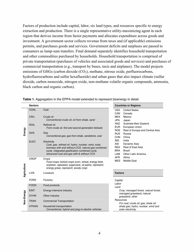
As represented in Figure 2, production of each biofuel crop is represented by a series of nested CES functions. For sugarcane, energy grass and woody crops, soil carbon credits are produced as a co-product with biofuel feedstocks. The nesting structure facilitates endogenous yield responses to changes in land prices by allowing substitution between land and the energy-materials composite (e.g., fertilizer) and between the resource-intensive bundle and the capital-labor aggregate. The model also includes exogenous yield improvements of 1% per year for all crops (including food crops). Benchmark yields for each first generation biofuel crop in each region are calculated as production-weighted averages of observed yields by country from FAOSTAT (2013) and are reported in Table 2. As FAOSTAT provides yields for palm oil fruit, palm oil per hectare will depend on extraction rates. Guided by statistics from the Malaysian Palm Oil Board (see http://bepi.mpob.gov.my/), we specify a yield of four metric tons of palm oil per hectare for Dynamic Asia (ASI). We calculate yields for other regions based on their palm fruit oil yields relative to Dynamic Asia.1

Biofuel feedstocki Carbon creditj

If j = Sugarcane, energy grass or wood crop

𝜎!!!"!

Resource-intensive Capital-Labor

𝜎!!!"! 𝜎!!!!

Land Energy-Materials Capital

𝜎!!!!

Aggregate energy Intermediate inputs

𝜎!!!"! 𝜎!!

Electricity Other energy Input1 ………. InputN

𝜎!"!

Coal Oil Gas Refined oil

Figure 2. Bioenergy crop production (j = corn, sugarcane, sugar beet, wheat, palm fruit, rapeseed, soybean, energy grass, woody crop).

1 Although almost all crops are produced in all regions, production of some crops is limited in some regions. For example, the European Union (EUR) has relatively high yields for sugarcane, but produces only a small amount. Based on production data from FAOSTAT (2013), we represent these constraints by excluding or limiting production of sugarcane in the EU and the US, and all first-generation bioenergy crops in the Middle East.

7

Table 2. Bioenergy crop yields, wet metric tons per hectare per year (unless stated otherwise). USA CAN MEX BRA LAM EUR RUS ROE CHN IND JPN ASI REA ANZ MES AFR Corn 9.5 8.5 3.2 3.8 5.9 5.0 2.9 4.8 5.2 2.3 2.6 3.4 3.6 6.2 7.0 1.7 Rapeseed 1.4 1.5 1.3 1.3 2.2 2.5 1.2 1.3 1.9 1.1 1.2 1.2 0.9 1.0 2.1 1.2 Soybean 2.8 2.3 1.4 2.8 2.9 1.4 0.9 1.4 1.5 1.2 1.6 1.4 1.4 2.4 2.4 1.0 Sugar beet 63.2 55.2 0.0 0.0 76.6 47.0 29.2 35.1 41.3 0.0 64.5 0.0 41.7 0.0 36.8 51.3 Sugarcane 78.0 - 75.4 77.6 78.9 80.3 - - 71.2 69.0 67.9 68.7 53.5 83.3 86.9 59.0 Wheat 2.7 2.3 5.1 2.2 2.9 3.4 2.1 2.3 4.6 2.7 4.3 3.5 2.5 1.1 2.5 2.0 Palm fruit - - 12.3 10.6 18.1 - - - 13.9 - - 19.0 - - - 3.8 Energy grass* 16.8 12.7 14.0 42.5 42.5 14.7 11.3 14.8 9.4 8.8 14.8 41.5 13.2 16.0 6.8 15.5 Woody crop* 12.3 8.2 13.4 21.1 21.1 12.3 8.2 12.3 9.4 8.5 9.2 15.9 10.5 15.9 4.9 14.6

* Oven dry metric tons per year. Source: Yields for all crops except energy grasses and woody crops are sourced from FAOSTAT (2013). Yields for

energy grasses and woody crops in the US are based on a literature survey. Yields for these crops in other regions are calculated by applying yield adjust factors to US yields calculated using the TEM for the energy grass and Brown (2000) for the woody crop.

For the energy grass, we assign yields in the US and multiply by adjustment factors from the Terrestrial Ecosystem Model (TEM, see http://ecosystems.mbl.edu/tem/) to estimate yields for other regions. Using a process-level agroecosystem model, Thomson et al. (2009) estimate that on all continental US cropland, switchgrass—an important energy crop—yields an average of 5.6 oven dry tons (ODT) per ha. Schmer et al. (2008) observed switchgrass yields of 5.2–11.1 ODT/ha in field trials on marginal cropland in the mid-continental US, and McLaughlin and Kszos (2005) observed yields from 18 field sites in 13 states ranging from 9.9–23.0 ODT/ha, with an average of 13.4 ODT/ha (Heaton et al., 2008). For Miscanthus, another important potential energy crop, Lewandowski et al. (2000) report results from field trials on unirrigated land in Southern Europe of 10–25 t/ha. Heaton et al. (2008) compared Miscanthus and switchgrass in side-by-side field trials in Illinois and observed average yields of 30 t/ha for Miscanthus and 10t/ha for switchgrass. Based on this literature, we assign a US yield of 16.8 ODT/ha for the representative energy grass. To calculate energy grass yields for other regions, we multiply the US yield by net primary productivity for C3-C4 grasslands estimated by the TEM in each region divided by that in the US. Energy grass yields for Brazil and Other Latin America (listed in Table 2) are higher than yields typically estimated for energy grasses in the US, but are consistent with the findings of Morais et al. (2009), in which yields for elephant grass (Pennisetum purpureum Schum.) were observed at 45–67 ODT/ha in trials at the Embrapa Agrobiologia field station in Brazil. For the woody crop, we assign a yield of 12.3 ODT/ha in the US and calculate yield adjustment parameters for other regions based on forestry yields reported in Brown (2000, Tables 6 and 7).

Calibration of production activities for biofuel feedstocks requires assigning cost shares per gasoline-equivalent gallon (GEG) for each pathway. We calculate land costs per GEG by combining the crop yields in Table 2 with estimates of feedstock requirements per GEG of fuel and land rents. Feedstock requirements are based on a literature survey and are displayed in Table 3. Land rental costs per hectare are calculated using data on total land rents from the

8

GTAP database and land-use estimates from the TEM. Costs for other crop production inputs are sourced from the GTAP database for first-generation crops, and from Duffy (2008) for energy grasses. For corn, rapeseed, soybean and wheat, we also track residues that can be sustainably removed and used as feedstock for LC ethanol. Residues are produced in fixed proportion to the output of each crop, and are calculated by applying residue ratios, retention shares and energy contents from Gregg and Smith (2010).

For soil carbon accumulation, we assume that sugarcane, energy grass and woody crop accumulate, respectively, 3.7, 1.8 and 3.3 metric tons of CO2 per hectare (ha) per year. These numbers are based on estimates by Cerri et al. (2011) for sugarcane, Anderson-Teixeira et al. (2009) for energy grass, and the Forest and Agricultural Sector Optimization Model with GHGs (FASOM-GHG) for woody crops.

Table 3. Bioenergy conversion requirements and co-products.

Technology Energy conversion requirement Co-product(s) Corn ethanol 31.0 lb per GEG 9.5 lb of DDGS per GEG Sugarcane ethanol 190.7 lb per GEG Electricity Sugarbeet ethanol 125.0 lb per GEG - Wheat ethanol 33.2 lb per GEG 9.9 lb of DDGS per GEG Palm oil diesel 42.4 lb per GEG - Rapeseed diesel 17.9 lb per GEG 9.7 lb of meal per GEG Soybean diesel 36.4 lb per GEG 28.8 lb of meal per GEG LC ethanol 40% energy conversion efficiency Electricity LC drop-in fuel 35% energy conversion efficiency Electricity

Biofueli Co-producti

𝜎!"#!!!

K-L-Intermediates Biofuel feedstocki 𝜎!"!!!

Capital-Labor Intermediate inputs 𝜎!!!! 𝜎!!

Capital Labor Input1 ………….. InputN

Figure 3. Biofuel production (i = corn ethanol, sugarcane ethanol, sugar beet ethanol, wheat ethanol, palm oil diesel, rapeseed diesel, soybean diesel, LC ethanol, LC drop-in fuel).

Shown in Figure 3, production functions for each biofuel combine inputs of pathway-specific feedstocks and other inputs, including capital, labor and intermediate inputs. For first-generation biofuels, we set the elasticity of substitution between the biofuel feedstock and other inputs (𝜎!"#!!! ) equal to zero, so a fixed quantity of feedstock is needed per GEG of fuel. For second-generation

9

pathways, we assign a positive value for 𝜎!"#!!! , allowing producers to respond to relative prices by extracting more energy per ton of feedstock at an increasing marginal cost.

Some processes also produce other co-products in addition to biofuel. Output from these sectors is modeled using a joint production function, where fuel and co-products are produced in fixed proportions. Co-products represented include distiller's dried grains with solubles (DDGS) for corn and wheat ethanol, electricity for sugarcane ethanol, LC ethanol and LC drop-in fuel, and meal for soybean and rapeseed diesel. Non-electricity biofuel co-products substitute for output from the crops sector, and electricity co-products substitute for output from the electricity sector. Co-products produced per GEG for each fuel are described in Table 3.

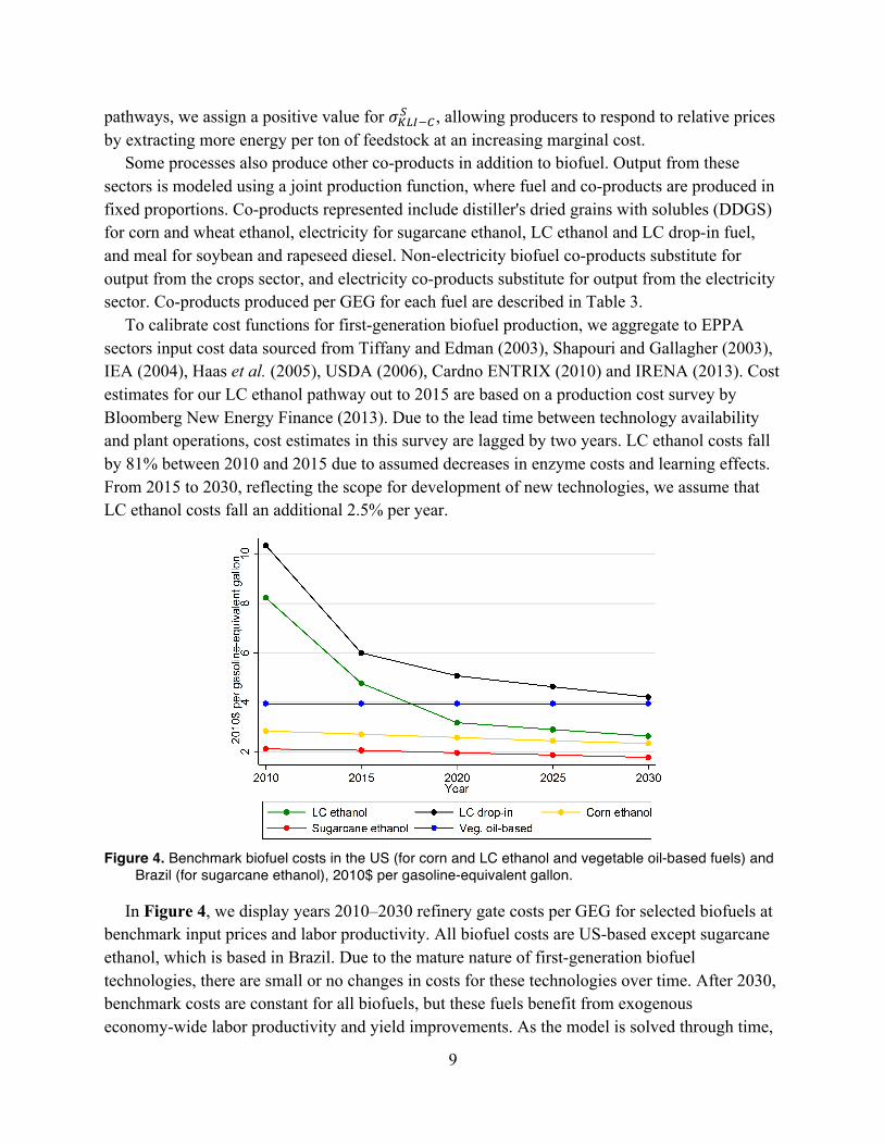
To calibrate cost functions for first-generation biofuel production, we aggregate to EPPA sectors input cost data sourced from Tiffany and Edman (2003), Shapouri and Gallagher (2003), IEA (2004), Haas et al. (2005), USDA (2006), Cardno ENTRIX (2010) and IRENA (2013). Cost estimates for our LC ethanol pathway out to 2015 are based on a production cost survey by Bloomberg New Energy Finance (2013). Due to the lead time between technology availability and plant operations, cost estimates in this survey are lagged by two years. LC ethanol costs fall by 81% between 2010 and 2015 due to assumed decreases in enzyme costs and learning effects. From 2015 to 2030, reflecting the scope for development of new technologies, we assume that LC ethanol costs fall an additional 2.5% per year.

Figure 4. Benchmark biofuel costs in the US (for corn and LC ethanol and vegetable oil-based fuels) and Brazil (for sugarcane ethanol), 2010$ per gasoline-equivalent gallon.

In Figure 4, we display years 2010–2030 refinery gate costs per GEG for selected biofuels at benchmark input prices and labor productivity. All biofuel costs are US-based except sugarcane ethanol, which is based in Brazil. Due to the mature nature of first-generation biofuel technologies, there are small or no changes in costs for these technologies over time. After 2030, benchmark costs are constant for all biofuels, but these fuels benefit from exogenous economy-wide labor productivity and yield improvements. As the model is solved through time,

10

production costs are calculated endogenously based on changes in input prices, including changes in land rents and energy prices. We assume that conversion technologies are the same in all regions but that feedstock costs vary regionally according to differences in yields and land rents. Consequently, differences in land costs per GEG of fuel ultimately drive differences in biofuel production costs across regions.

As the uptake of ethanol will be limited by constraints on blending ethanol with gasoline and on ethanol use in some transportation modes (see Section 3.3), we also include an ethanol-to-diesel technology. Guided by Harvey and Meylemans (2014) and Staples et al. (2014), we assume that the cost of upgrading ethanol to diesel is $0.8 per gallon of diesel ($0.704 per GEG of diesel) and the energetic conversion efficiency when converting ethanol to diesel is 95%. This technology is able to upgrade both LC and first-generation ethanol.

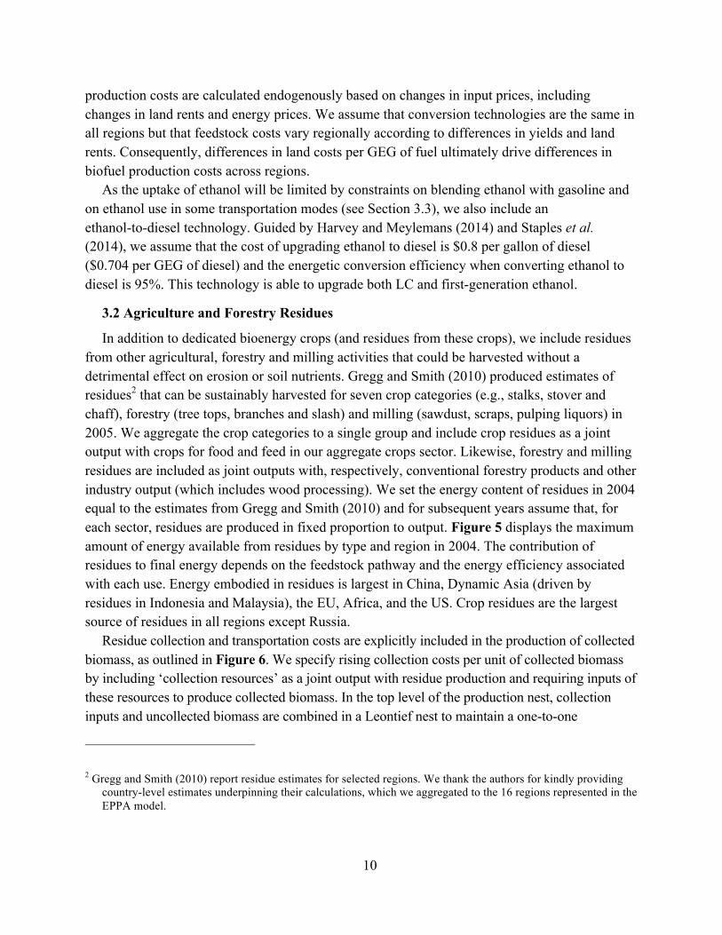
3.2 Agriculture and Forestry Residues

In addition to dedicated bioenergy crops (and residues from these crops), we include residues from other agricultural, forestry and milling activities that could be harvested without a detrimental effect on erosion or soil nutrients. Gregg and Smith (2010) produced estimates of residues2 that can be sustainably harvested for seven crop categories (e.g., stalks, stover and chaff), forestry (tree tops, branches and slash) and milling (sawdust, scraps, pulping liquors) in 2005. We aggregate the crop categories to a single group and include crop residues as a joint output with crops for food and feed in our aggregate crops sector. Likewise, forestry and milling residues are included as joint outputs with, respectively, conventional forestry products and other industry output (which includes wood processing). We set the energy content of residues in 2004 equal to the estimates from Gregg and Smith (2010) and for subsequent years assume that, for each sector, residues are produced in fixed proportion to output. Figure 5 displays the maximum amount of energy available from residues by type and region in 2004. The contribution of residues to final energy depends on the feedstock pathway and the energy efficiency associated with each use. Energy embodied in residues is largest in China, Dynamic Asia (driven by residues in Indonesia and Malaysia), the EU, Africa, and the US. Crop residues are the largest source of residues in all regions except Russia.

Residue collection and transportation costs are explicitly included in the production of collected biomass, as outlined in Figure 6. We specify rising collection costs per unit of collected biomass by including ‘collection resources’ as a joint output with residue production and requiring inputs of these resources to produce collected biomass. In the top level of the production nest, collection inputs and uncollected biomass are combined in a Leontief nest to maintain a one-to-one

2 Gregg and Smith (2010) report residue estimates for selected regions. We thank the authors for kindly providing country-level estimates underpinning their calculations, which we aggregated to the 16 regions represented in the EPPA model.

11

relationship between the energy content of uncollected and collected residues. Collection inputs are an aggregate of capital, labor, transportation and collection resources, which are produced in fixed proportion to uncollected residues. Specifically, 𝛿! (0 < 𝛿! <1) collection resources are produced for each unit of residues and 𝛿! collection resources are required per unit of collected biomass. If 𝛿!< 𝛿! , the proportion of residues that can be collected at the base cost is determined by 𝛿! 𝛿! , and additional residues can only be collected at a higher cost. The shape of the ‘supply curve’ for collected residues is driven by the elasticity of substitution between collection resources and other inputs (𝜎!"). Guided by residue supply curves estimated by Gallagher et al. (2003) and USDA (2011), we set 𝜎!" equal to 0.9, 𝛿!  = 1 and 𝛿! = 0.1.

Figure 5. Residue biomass potential by type and region in 2004 (EJ). Source: Authors’ aggregation of

estimates from Gregg and Smith (2010).

Figure 6. Production of collected biomass residues.

Collected Residues 𝜎!" = 0

Collection Inputs Uncollected Residues

𝜎!" Collection Resource Transportation-KL

𝜎!"# Capital-Labor Transport 𝜎!"

Capital Labor

12

3.3 Changes in Land Use

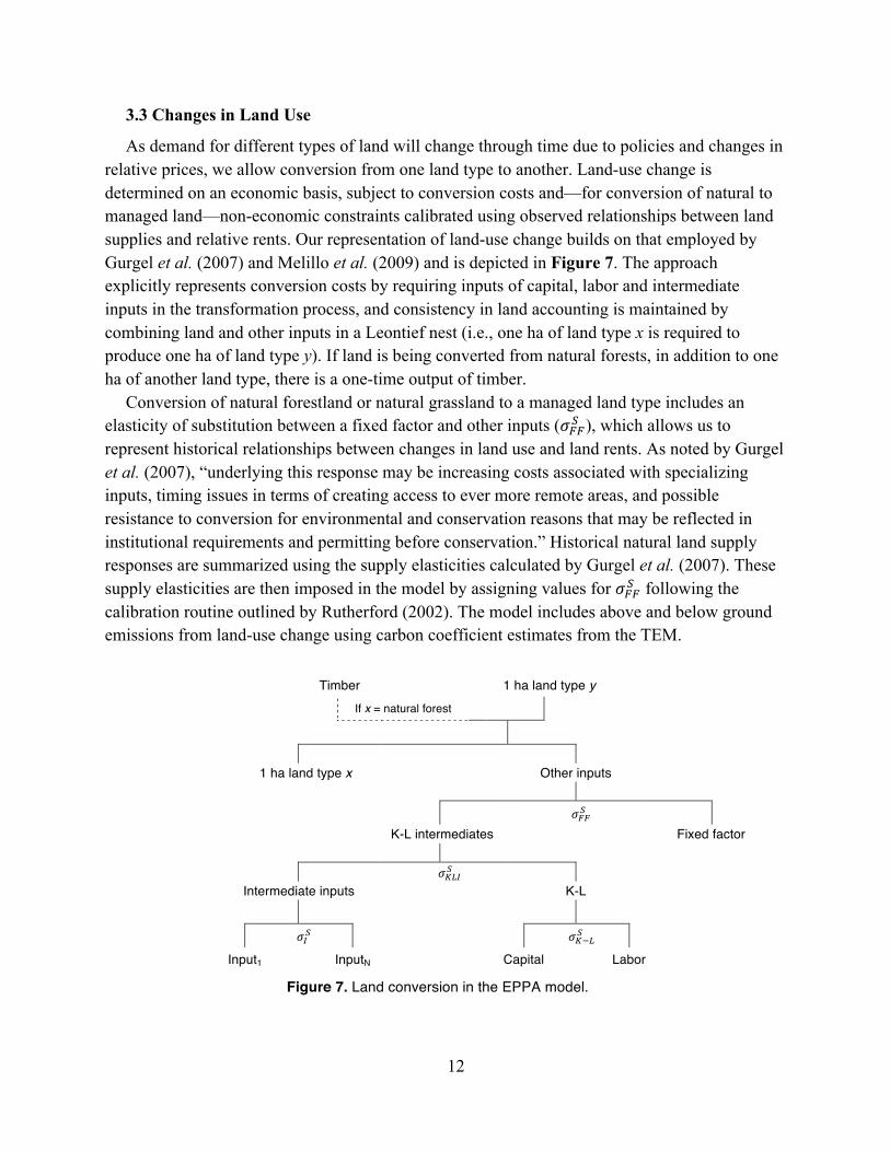
As demand for different types of land will change through time due to policies and changes in relative prices, we allow conversion from one land type to another. Land-use change is determined on an economic basis, subject to conversion costs and—for conversion of natural to managed land—non-economic constraints calibrated using observed relationships between land supplies and relative rents. Our representation of land-use change builds on that employed by Gurgel et al. (2007) and Melillo et al. (2009) and is depicted in Figure 7. The approach explicitly represents conversion costs by requiring inputs of capital, labor and intermediate inputs in the transformation process, and consistency in land accounting is maintained by combining land and other inputs in a Leontief nest (i.e., one ha of land type x is required to produce one ha of land type y). If land is being converted from natural forests, in addition to one ha of another land type, there is a one-time output of timber.

Conversion of natural forestland or natural grassland to a managed land type includes an elasticity of substitution between a fixed factor and other inputs (𝜎!!! ), which allows us to represent historical relationships between changes in land use and land rents. As noted by Gurgel et al. (2007), “underlying this response may be increasing costs associated with specializing inputs, timing issues in terms of creating access to ever more remote areas, and possible resistance to conversion for environmental and conservation reasons that may be reflected in institutional requirements and permitting before conservation.” Historical natural land supply responses are summarized using the supply elasticities calculated by Gurgel et al. (2007). These supply elasticities are then imposed in the model by assigning values for 𝜎!!! following the calibration routine outlined by Rutherford (2002). The model includes above and below ground emissions from land-use change using carbon coefficient estimates from the TEM.

Timber 1 ha land type y If x = natural forest

1 ha land type x Other inputs

𝜎!!!

K-L intermediates Fixed factor

𝜎!"#!

Intermediate inputs K-L

𝜎!! 𝜎!!!!

Input1 InputN Capital Labor

Figure 7. Land conversion in the EPPA model.

13

3.4 Other Bioenergy Features

Our analysis also augments several other features of the EPPA model in order to facilitate a detailed representation of bioenergy. First, several existing policies promoting biofuel were added to the model for inclusion in the study. These additions include renewable fuel standards in the EU and the US and estimates of how these policies may evolve in the future. To capture the EU policy, we impose minimum shares of renewable fuel in the transport sector of 5.75% in 2010, 10% in 2020 and 13.5% in 2030 and beyond. Additionally, to reflect a 2012 proposal by the European Commission, we constrain fuel produced using food crops to a maximum of 50% of the EU mandates from 2015 onwards. For the US, for 2010, 2015 and 2020, we impose the minimum volumetric targets for biomass-based diesel, cellulosic biofuels, undifferentiated advanced biofuel and total renewable fuel outlined in the Energy Independence and Security Act of 2007. As targets are not specified beyond 2022, we convert the volumetric targets in 2022 to proportions of total transportation fuel and impose these targets into the future. In the model, the constraints are imposed using a permit system, as depicted in Figure 8. One permit is issued for each GEG of renewable fuel produced, and retailers of both conventional fuel and renewable fuel are required to surrender 𝛼 (set exogenously; 0 < 𝛼 < 1) permits for each GEG of fuel sold. Under such a system, 𝛼  determines the share of renewable fuel in total fuel consumption. This procedure can be used to target volumetric biofuel mandates by solving the model iteratively for alternative values of 𝛼. For the US, we include a separate permit system for each fuel type mandated.

(a) (b)

Figure 8. Production and blending of renewable fuel permits into (a) Conventional fuel and (b) Biofuels.

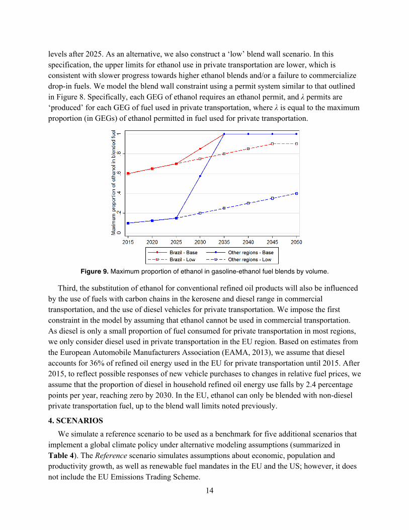
Second, the consumption of ethanol in each time period and region may be limited by the ability of the prevailing infrastructure and vehicle fleet to absorb this fuel, commonly known as the ‘blend wall’. We consider two blend wall cases applied to aggregate fuel purchases, which are illustrated in Figure 9. In our core scenario, we assume a ‘base’ blend wall case. In Brazil, we set an upper limit for ethanol in blended gasoline of 60% in 2015 (based on predicted sales and current stocks of flexible-fuel vehicles and vehicles able to accept blended fuel containing up to 25% ethanol). This upper limit is relaxed over time to reflect greater penetration of flex-fuel vehicles and the availability of molecules that can be blended to higher levels in gasoline (e.g., butanol and drop-in gasoline), so by 2035 there is no blend wall constraint. For other regions, we assume slower progress towards the use of 15% and 20% fuel blends between 2010 and 2025, but greater acceptance of ethanol and/or development of molecules that can be blended to higher

1  gal.  fuel  

α  Permits  

1  gal.  Conventional  fuel  

1  gal.  Fuel 1  Permit  

α  Permits  

1  gal.  Biofuel  

14

levels after 2025. As an alternative, we also construct a ‘low’ blend wall scenario. In this specification, the upper limits for ethanol use in private transportation are lower, which is consistent with slower progress towards higher ethanol blends and/or a failure to commercialize drop-in fuels. We model the blend wall constraint using a permit system similar to that outlined in Figure 8. Specifically, each GEG of ethanol requires an ethanol permit, and λ permits are ‘produced’ for each GEG of fuel used in private transportation, where λ is equal to the maximum proportion (in GEGs) of ethanol permitted in fuel used for private transportation.

Figure 9. Maximum proportion of ethanol in gasoline-ethanol fuel blends by volume.

Third, the substitution of ethanol for conventional refined oil products will also be influenced by the use of fuels with carbon chains in the kerosene and diesel range in commercial transportation, and the use of diesel vehicles for private transportation. We impose the first constraint in the model by assuming that ethanol cannot be used in commercial transportation. As diesel is only a small proportion of fuel consumed for private transportation in most regions, we only consider diesel used in private transportation in the EU region. Based on estimates from the European Automobile Manufacturers Association (EAMA, 2013), we assume that diesel accounts for 36% of refined oil energy used in the EU for private transportation until 2015. After 2015, to reflect possible responses of new vehicle purchases to changes in relative fuel prices, we assume that the proportion of diesel in household refined oil energy use falls by 2.4 percentage points per year, reaching zero by 2030. In the EU, ethanol can only be blended with non-diesel private transportation fuel, up to the blend wall limits noted previously.

4. SCENARIOS

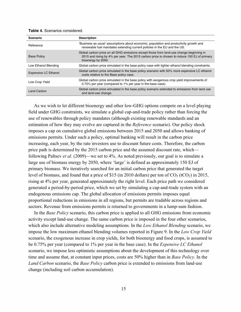
We simulate a reference scenario to be used as a benchmark for five additional scenarios thatimplement a global climate policy under alternative modeling assumptions (summarized in Table 4). The Reference scenario simulates assumptions about economic, population and productivity growth, as well as renewable fuel mandates in the EU and the US; however, it does not include the EU Emissions Trading Scheme.

15

Table 4. Scenarios considered.

Scenario Description

Reference ‘Business as usual’ assumptions about economic, population and productivity growth and renewable fuel mandates extending current policies in the EU and the US.

Base Policy Global carbon price on all GHG emissions except those from land-use change beginning in

2015 and rising by 4% per year. The 2015 carbon price is chosen to induce 150 EJ of primary bioenergy by 2050.

Low Ethanol Blending Global carbon price simulated in the base policy case with tighter ethanol blending constraints.

Expensive LC Ethanol Global carbon price simulated in the base policy scenario with 50% more expensive LC ethanol costs relative to the Base policy case.

Low Crop Yield Global carbon price simulated in the base policy with exogenous crop yield improvements of 0.75% per year (compared to 1% per year in the base case).

Land Carbon Global carbon price simulated in the base policy scenario extended to emissions from land use and land-use change.

As we wish to let different bioenergy and other low-GHG options compete on a level playing field under GHG constraints, we simulate a global cap-and-trade policy rather than forcing the use of renewables through policy mandates (although existing renewable standards and an estimation of how they may evolve are captured in the Reference scenario). Our policy shock imposes a cap on cumulative global emissions between 2015 and 2050 and allows banking of emissions permits. Under such a policy, optimal banking will result in the carbon price increasing, each year, by the rate investors use to discount future costs. Therefore, the carbon price path is determined by the 2015 carbon price and the assumed discount rate, which—following Paltsev et al. (2009)—we set to 4%. As noted previously, our goal is to simulate a large use of biomass energy by 2050, where ‘large’ is defined as approximately 150 EJ of primary biomass. We iteratively searched for an initial carbon price that generated the target level of biomass, and found that a price of $15 (in 2010 dollars) per ton of CO2 (tCO2) in 2015, rising at 4% per year, generated approximately the right level. Each price path we considered generated a period-by-period price, which we set by simulating a cap-and-trade system with an endogenous emissions cap. The global allocation of emissions permits imposes equal proportional reductions in emissions in all regions, but permits are tradable across regions and sectors. Revenue from emissions permits is returned to governments in a lump-sum fashion.

In the Base Policy scenario, this carbon price is applied to all GHG emissions from economic activity except land-use change. The same carbon price is imposed in the four other scenarios, which also include alternative modeling assumptions. In the Low Ethanol Blending scenario, we impose the low maximum ethanol blending volumes reported in Figure 9. In the Low Crop Yield scenario, the exogenous increase in crop yields, for both bioenergy and food crops, is assumed to be 0.75% per year (compared to 1% per year in the base case). In the Expensive LC Ethanol scenario, we impose less optimistic assumptions about the development of this technology over time and assume that, at constant input prices, costs are 50% higher than in Base Policy. In the Land Carbon scenario, the Base Policy carbon price is extended to emissions from land-use change (including soil carbon accumulation).

16

As modeling assumptions in some policy scenarios differ from those in the Reference scenario, we implement separate reference scenarios for the Low Ethanol Blending, Low Crop Yield and Expensive LC Ethanol policy cases. These reference scenarios differ from the core Reference scenario in that we have included the alternative assumption examined in each policy case (e.g., the reference scenario for the Low Crop Yield scenario imposes the same business-as-usual assumptions and RFS policies as in the core Reference case, plus the crop yield assumptions in the Low Crop Yield case). Results for these additional reference scenarios are not reported, but are used to calculate relative changes in the relevant policy scenarios. For each policy scenario, we also simulate the carbon price when bioenergy technologies are unavailable. Results for these simulations are also not reported, but we compare differences between results to quantify the independent impacts of using biomass to produce energy.

5. RESULTS

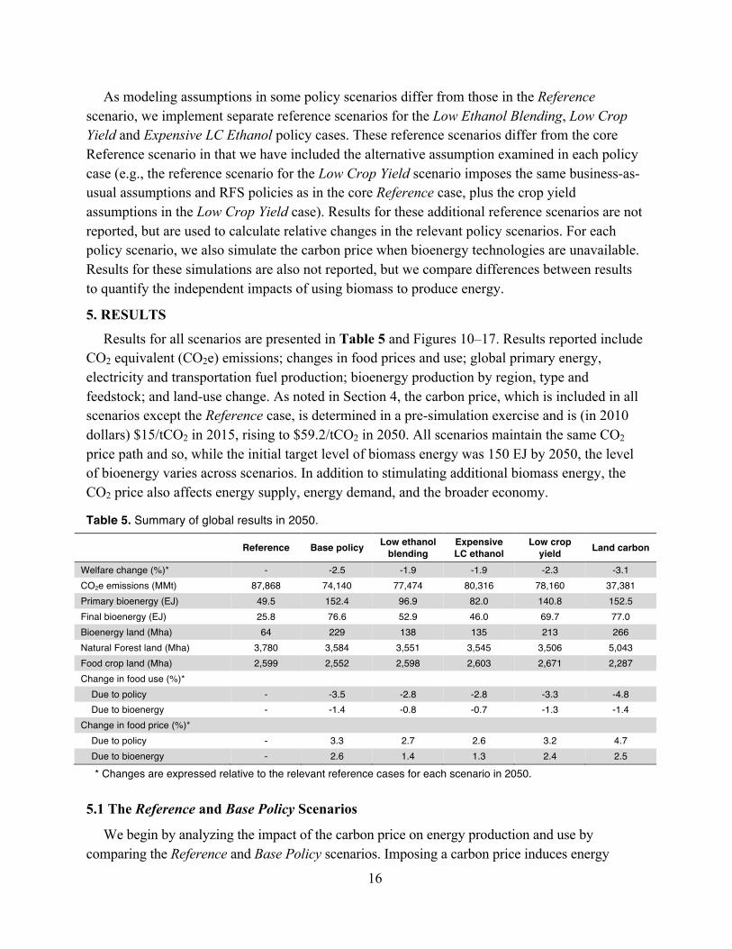
Results for all scenarios are presented in Table 5 and Figures 10–17. Results reported includeCO2 equivalent (CO2e) emissions; changes in food prices and use; global primary energy, electricity and transportation fuel production; bioenergy production by region, type and feedstock; and land-use change. As noted in Section 4, the carbon price, which is included in all scenarios except the Reference case, is determined in a pre-simulation exercise and is (in 2010 dollars) $15/tCO2 in 2015, rising to $59.2/tCO2 in 2050. All scenarios maintain the same CO2 price path and so, while the initial target level of biomass energy was 150 EJ by 2050, the level of bioenergy varies across scenarios. In addition to stimulating additional biomass energy, the CO2 price also affects energy supply, energy demand, and the broader economy.

Table 5. Summary of global results in 2050.

Reference Base policy Low ethanol blending

Expensive LC ethanol

Low crop yield Land carbon

Welfare change (%)* - -2.5 -1.9 -1.9 -2.3 -3.1 CO2e emissions (MMt) 87,868 74,140 77,474 80,316 78,160 37,381 Primary bioenergy (EJ) 49.5 152.4 96.9 82.0 140.8 152.5 Final bioenergy (EJ) 25.8 76.6 52.9 46.0 69.7 77.0 Bioenergy land (Mha) 64 229 138 135 213 266 Natural Forest land (Mha) 3,780 3,584 3,551 3,545 3,506 5,043 Food crop land (Mha) 2,599 2,552 2,598 2,603 2,671 2,287 Change in food use (%)* Due to policy - -3.5 -2.8 -2.8 -3.3 -4.8 Due to bioenergy - -1.4 -0.8 -0.7 -1.3 -1.4 Change in food price (%)* Due to policy - 3.3 2.7 2.6 3.2 4.7 Due to bioenergy - 2.6 1.4 1.3 2.4 2.5

* Changes are expressed relative to the relevant reference cases for each scenario in 2050.

5.1 The Reference and Base Policy Scenarios

We begin by analyzing the impact of the carbon price on energy production and use by comparing the Reference and Base Policy scenarios. Imposing a carbon price induces energy

17

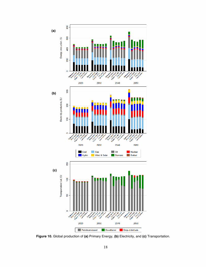
efficiency improvements and energy use reductions, resulting in global primary energy use of 573.6 EJ in 2050 (compared to 718.7 EJ in the Reference scenario) (Figure 10a). The carbon price also reduces energy from coal and oil, and promotes energy from low-carbon sources, especially biomass. Similar changes are observed for electricity (Figure 10b). In 2050, the Base Policy scenario shows 19% less electricity consumption and 73% less electricity from coal (relative to Reference). Biomass electricity and electricity produced as a co-product with biofuels reach a combined total of 11 EJ, or 9% of total production (compared to 0.9 EJ in the Reference scenario). Transportation fuels are also affected (Figure 10c). In 2050, the Base Policy total transportation fuel use is 10% less (relative to Reference), ethanol accounts for 93% of global private transportation fuel energy use, and from 2015–2050 the biofuels share of total transportation fuels rises from 3% to 38% (whereas in the Reference scenario, it rises to just 11%).

In the Base Policy case, greater use of biomass and other abatement options decrease total GHG emissions by 16% relative to Reference (see Table 5). Base Policy cumulative GHG emissions from 2015–2050 are 1.3 trillion metric tons. IPCC estimates (IPCC, 2013, Table SPM.10) indicate that this level of CO2 emissions through 2050 corresponds with a global mean surface temperature increase of ~2 degrees Celsius (°C) relative to the 1861–1800 average. If annual emissions from 2051 to 2100 are held constant at the 2050 level, cumulative 2015–2100 CO2 emissions are 3 trillion metric tons, which corresponds with a total increase of ~3°C. Net of climate benefits, the Base Policy carbon price reduces global welfare in 2050 by 2.5% relative to the Reference case, where welfare changes are measured as equivalent variation changes in consumption spending.

In the Reference scenario, driven by renewable fuel mandates in the EU and the US and the cost competitiveness of some biomass technologies, primary bioenergy rises from 8.5 EJ in 2015 to 49.5 EJ in 2050. Bioenergy production in 2050 includes bioheat, sugarcane, and LC ethanol. Corn ethanol and diesel from soybean and palm oil are produced only until 2025. The increase in biomass energy over time is mainly driven by increases in fossil fuel prices and cost reductions for LC ethanol.

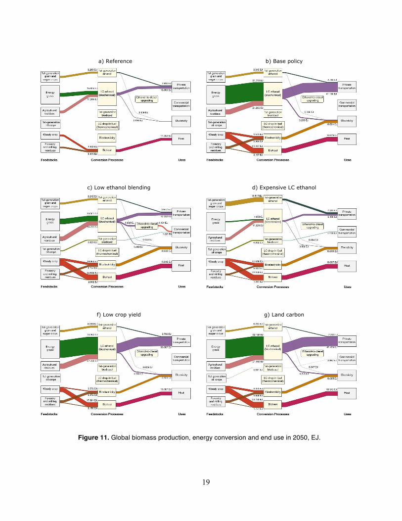
In the Base Policy, primary bioenergy increases to 152.4 EJ in 2050 (predetermined by our ~150 EJ target), or 76.6 EJ of final energy (Figures 11 & 12). In this scenario, the ethanol blending constraint is binding from 2015 to 2025, which results in ethanol being upgraded to diesel in these years. Corn ethanol is produced in the US up until 2025, when it becomes uneconomical. After 2025, higher limits on ethanol in gasoline blends remove the need to upgrade ethanol to diesel, and in 2050 LC ethanol accounts for around 57% of total bioenergy consumption by energy content.3

3 Assuming LC ethanol plant capacity of 135 million gallons per year, LC ethanol production simulated in the Base Policy scenario requires a global average build rate of 36 new plants per year from 2015–2030, and 160 new plants per year from 2035–2050. For comparison, 31 first-generation ethanol plants were built in the US in 2009 and 30 in Brazil in 2008 (RFA, 2014; GAIN, 2013).

18

Figure 10. Global production of (a) Primary Energy, (b) Electricity, and (c) Transportation.

(b)

(a)

(c)

19

a) Reference b) Base policy

c) Low ethanol blending d) Expensive LC ethanol

f) Low crop yield g) Land carbon

Figure 11. Global biomass production, energy conversion and end use in 2050, EJ.

20

Figure 12. Global final bioenergy by energy type.

The carbon price induces other price changes that make LC ethanol the cheapest biofuel in most regions. Energy grass requires less energy-intensive inputs than first-generation crops, and thus is less affected by rising energy prices, and as LC ethanol has lower land costs per GEG than other biofuels, rising land prices also have a smaller impact on LC ethanol. Additionally, rising electricity prices will increase LC ethanol’s co-product revenue.4

Other major sources of bioenergy production in the Base Policy scenario include bioheat and bioelectricity (produced from dedicated bioelectricity operations and as a co-product with biofuels). Bioelectricity production is driven by relatively large increases in the carbon-cost-inclusive price of coal. LC drop-in fuels are not produced due to their relatively high costs, and CCS is not economical in any year for any technology. When the carbon price is first introduced, most bioenergy is produced from the woody crop, but energy grass becomes the largest source of bioenergy by 2035 (Figure 13). By 2050, forestry and agricultural residues combined account for 15.6 EJ (or 20%) of final bioenergy.

The largest bioenergy producers in the Base Policy scenario are Africa (15.4 EJ of final bioenergy) and Brazil (11.1 EJ) (see Figure 14). Most bioenergy produced in Africa in 2050 is LC ethanol with electricity produced as a co-product. In Brazil, bioenergy production is split between LC and sugarcane ethanol (with electricity co-product) and bioheat. Other major bioenergy production regions include China, which produces LC ethanol and bioelectricity; Other Latin

4 With low energy-intensive inputs, LC drop-in fuels and sugarcane ethanol also benefit from rising electricity co-product revenue. However, LC drop-in fuels remain more expensive than LC ethanol. When the blend wall is binding, LC drop-in fuels are also more expensive than upgrading ethanol to diesel.

21

Figure 13. Global final bioenergy production by feedstock.

Figure 14. Regional final bioenergy by scenario in 2050.

04

812

16B

ioen

ergy

, EJ

AFRBRA

CHNIN

DUSA

ANZEUR ASI

REALA

MMEX

CANROE

RUSMES

JPN

a) Reference

04

812

16B

ioen

ergy

, EJ

AFRBRA

CHNLA

MUSA

ASIRUS

MEXCAN

IND

ANZEUR

ROEREA

MESJP

N

b) Base policy

04

812

16B

ioen

ergy

, EJ

AFRCHN

BRARUS

LAM ASI

MEXCAN

IND

USAANZ

EURROE

REAMES

JPN

c) Low ethanol blending

04

812

16B

ioen

ergy

, EJ

CHNBRA

USARUS

LAM

AFR ASICAN

MEXANZ

IND

EURROE

REAMES

JPN

d) Expensive LC ethanol

04

812

16B

ioen

ergy

, EJ

AFRBRA

CHNLA

MUSA

ASIRUS

IND

MEXANZ

CANROE

EURREA

MESJP

N

e) Low crop yield

04

812

16B

ioen

ergy

, EJ

AFRCHN

BRALA

MANZ

USARUS

MEXCAN

IND ASI

EURROE

REAMES

JPN

f) Land carbon

Heat Electricity 1st gen. ethanol Veg. oil-based LC ethanol

22

America, which primarily produces LC ethanol and bioheat; and the US, which mostly produces LC ethanol. Sugarcane ethanol, produced in Brazil and Mexico, is the only first-generation biofuel still produced in 2050.

The carbon price and bioenergy production induce changes in land use (see Figures 15 & 16). In 2050, in the Reference case, global land use includes 2,599 million hectares (Mha) for food crops and 64 Mha for bioenergy crops; in the Base Policy scenario, food crops use 2,552 Mha and bioenergy crops use 229 Mha. The additional bioenergy cropland in the Base Policy scenario comes at the expense of food crops, and also natural forestland—natural forest area is 196 Mha lower than in the Reference case due to deforestation, mainly in Africa (101 Mha), Other Latin America (62 Mha) and Brazil (29 Mha) (Figure 17a).

Figure 15. Global land use, million ha. Note: Land unsuitable for growing vegetation is not represented.

Figure 16. Global land-use change relative to the reference scenario, million ha.

23

Figure 17. Regional land-use change relative to the Reference scenario in 2050, million ha.

Although global livestock production decreases, managed grassland (pasture) areas increase in the Base policy scenario relative to the Reference case due to a change in the regional composition of livestock production. The global change in managed grasslands is driven by a decrease in livestock production in Other Latin America and an increase in livestock production in Africa. Although pasture yields are higher in Other Latin America than Africa, the energy grass-to-pasture relative yield is also higher in this region. Following the theory of comparative advantage, this relative yield difference, ceteris paribus, promotes livestock production in Africa. As pasture yields are lower in Africa than in Other Latin America, livestock production decreases even though more land is allocated to pasture. There are also small increases in natural grassland in some regions, as this type of land is valued for its environmental services and the carbon price increases the relative cost of agricultural uses.

The impact of bioenergy on land-use change is influenced by at least three factors in our analysis. First, the scope for deforestation in the model reflects current trends and political constraints. Depending on how economic costs and incentives induced by a carbon price affect political and public opinion, there may be smaller or larger changes in land use. Second, some bioenergy feedstocks are sourced from forestry and agricultural residues. Third, improved efficiency both in growing crops and turning biomass into biofuel results in improvements in energy produced per ha of land. For example, in the US, the energy grass yield increases by 48% between 2015 and 2050, with 41 percentage points due to exogenous yield increases and the remainder due to a price-induced yield response. Combined with price-induced responses in

-200

020

0

Land

are

a, m

illion

ha

AFRLA

MBRA

ANZMEX

RUSUSA

CANROE

CHN ASIEUR

MESREA

IND

JPN

a) Base policy

-200

020

0

Land

are

a, m

illion

ha

AFRLA

MBRA

ANZRUS

MEXCAN

CHN ASIUSA

ROEEUR

MESREA

IND

JPN

b) Low ethanol blending

-200

020

0

Land

are

a, m

illion

ha

AFRLA

MBRA

ANZUSA

RUSMEX

CANCHN ASI

ROEEUR

MESREA

IND

JPN

c) Expensive LC ethanol

-200

020

0

Land

are

a, m

illion

ha

AFRLA

MBRA

ANZRUS

MEXUSA

CAN ASIROE

CHNMES

EURREA

IND

JPN

d) Low crop yield

-600

060

0

Land

are

a, m

illion

ha

AFRLA

MBRA

ANZROE ASI

REARUS

MEXUSA

CANEUR

MESCHN

IND

JPN

e) Land carbon

Food crops Bioenergy crops Managed grassland Managed forestNatural grassland Natural forest Wind energy

24

energy efficiency when converting grass into biofuel, each ha produces 51% more fuel in 2050 (1,757 GEGs per ha) than in 2015 (1,166 GEGs per ha).

Food use and prices are also affected (see Table 5).5 The carbon price decreases real incomes and the production of bioenergy drives up land prices. As a result, relative to the Reference case, in 2050 the Base Policy global food price increases by 3.3% and food use decreases by 3.5%. The reduction in food use is partially driven by a substitution effect, including using more other inputs so that food is used more efficiently (e.g., reducing waste); therefore, food use reduction percentages given do not solely represent reduction in calories consumed. We isolate the impact of bioenergy on food consumption and prices by imposing the carbon price when bioenergy technologies are unavailable, then compare the results to outcomes in the Base Policy case. This comparison indicates that bioenergy production alone increases food prices by 2.6% and decreases food consumption by 1.4%.

5.2 The Low Ethanol Blending Scenario

In this scenario, we impose tighter blend wall constraints to restrict the use of LC ethanol. Relative to the Base Policy case, this scenario decreases total bioenergy production, increases CO2e emissions, increases petroleum-based fuel use in transportation, and improves (net of climate benefits) welfare. A smaller decrease in welfare occurs, because tightening the blend wall constraint reduces changes in the economy relative to the Reference case, which by assumption was the optimal economic outcome (subject to prevailing constraints).6

Bioheat and dedicated bioelectricity production increase relative to the Base Policy case, although there is a decrease in total biomass electricity due to reduced production of electricity as a LC ethanol co-product. Ethanol-to-diesel upgrading and diesel from oil crops remain through 2050 due to the tighter blend wall constraints. In 2050, 23% of global ethanol production is upgraded to diesel, which results in 4.4 EJ of diesel from ethanol, and 1.2 EJ of palm oil diesel is produced in Dynamic Asia. As in the Base Policy case, LC drop-in fuels are never produced. In the Low Ethanol Blending scenario, all regions produce less final bioenergy relative to Base Policy, with the largest decrease occurring in Africa.

Less bioenergy production in the Low Ethanol Blending scenario reduces the amount of land used for energy crops. Changes in bioenergy crops and the regional composition of bioenergy drive differences in land-use change between the Base Policy and Low Ethanol Blending scenarios. Interestingly, although there is less land used for bioenergy crops in the Low Ethanol

5As our model, like all general equilibrium models, only resolves relative prices, we estimate food price changes using the relationship ∆𝐶 = 𝜖∆𝐼 + 𝜂∆𝑃, where ∆ denotes percentage change, 𝐶 is food consumption, 𝐼 is income, 𝑃 is the food price, and 𝜖 and 𝜂 are, respectively, the price and income elasticity of demand for food.

6 The opposite would be true under a cap on emissions rather than a fixed emissions price. That is, tightening the ethanol blending constraints under an emissions cap would increase the carbon price and ultimately result in a larger decrease in welfare.

25

Blending scenario, less land is also allocated to natural forests than in the Base Policy case. This is driven by linkages between food and bioenergy markets and interactions among regions. Specifically, relative to the Base Policy case and due to the tighter constraint on using fuel from the energy grass, China allocates more land to woody energy crops. As the woody crop yield in this region is less than that for the energy grass, more land is allocated to energy crops and less to food crops, which results in increased imports of food. A large share of these imports is sourced from Africa, where more land is allocated to food crops at the expense of natural forests due to relatively low political barriers to deforestation. This result indicates that, due to international agricultural trade, growing energy crops will reduce natural forest areas in regions with the lowest constraints to deforestation, regardless of the location of bioenergy production.

5.3 The Expensive LC Ethanol Scenario

In this scenario, we increase the cost of LC ethanol production. Similarly to Low Ethanol Blending, this change reduces total bioenergy production, increases CO2e emissions, and increases the use of petroleum-based fuels relative to the Base Policy case. The higher cost of LC ethanol also increases production of first-generation ethanol relative to other cases. In 2050, global ethanol production is 3.4 EJ from corn (mainly in the US) and 3.8 EJ from sugarcane (principally in Brazil), whereas global LC ethanol production is just 6.3 EJ (compared to 41.2 EJ in the Base Policy case). The blend wall is binding between 2015 and 2025, which induces production of LC drop-in fuels (1.4 EJ in 2025) and ethanol-to-diesel upgrading (0.9 EJ in 2025). From 2030 onward, the blend wall is not binding and LC drop-in and ethanol upgrading technologies do not operate.

Total bioenergy production in Africa falls by 78% relative to the Base Policy case, as increasing the cost of LC ethanol reduces production of this fuel (both for the domestic market and for export) and there is a large difference in energy yields for the energy grass and those for first-generation bioenergy crops in this region. China is the largest bioenergy producer in this scenario. Brazil and the US are also relatively large bioenergy producers due to their production of first-generation ethanol.

Similar to the Low Ethanol Blending scenario, less land is allocated to natural forests than in the Base Policy case due to increased production of food crops in Africa for export to China. Changes in food prices and use when LC ethanol is expensive are also smaller than in the Base Policy case.

5.4 The Low Crop Yield Scenario

In the Low Crop Yield scenario, the exogenous increase in crop yields is 0.75% per year (compared to 1% in all other scenarios). LC ethanol, bioheat and bioelectricity continue to be the major forms of bioenergy, but less total bioenergy is produced than in the Base Policy case. Compared to the Low Ethanol Blending and Expensive LC Ethanol scenarios, there is more total bioenergy and LC ethanol, but less first-generation ethanol. Driven by changes in total bioenergy production, CO2e emissions in the Low Crop Yield scenario are greater than those in the Base

26

Policy case, but less than emissions in the Low Ethanol Blending and Expensive LC Ethanol scenarios.

Although, relative to the Base Policy scenario, less land is used for bioenergy crops, less land is also allocated to natural forests in this scenario. This is because more land is used for food crops when yields are lower in both the Reference case and when there is a carbon price. For example, in 2050 at the global level, 2,599 Mha of land are used for food crops in the Reference scenario when yields increase by 1% per year, and 2,707 Mha are allocated to food crops in the this scenario when yields increase by 0.75% per year. As the amount of land used for bioenergy in the Low Crop Yield scenario is similar to the Base Policy case, changes in food prices (3.2%) and consumption (-3.4%) are also similar.

5.5 The Land Carbon Scenario

In this scenario, we price emissions from land use and land-use change to provide incentives for reforestation. However, soil carbon credits for some bioenergy crops counteract reforestation incentives, and bioenergy production in the Land Carbon scenario remains similar to that in the Base Policy case. Bioheat and bioelectricity increase while biofuels decrease, a change attributed to two related mechanisms. First, feedstock costs as a proportion of total costs for bioheat and bioelectricity are larger than those for biofuels, so decreasing (gross of carbon credits) feedstock costs has a larger impact on bioheat and bioelectricity. Second, although slightly more soil carbon is sequestered per ha of energy grass than woody crop, as woody crop yields are less than those for energy grass, woody crop provides more soil carbon credits per ton than energy grass. Ultimately, as woody crops are used for bioheat and bioelectricity but not for biofuels produced in the Land Carbon scenario, these forces result in larger cost decreases for bioheat and bioelectricity when land-use emissions are priced.

Pricing carbon from land-use change results in global reforestation of 800 Mha between 2010 and 2050—a significant increase from the Base Policy and Reference cases (1,459 Mha and 1,263 Mha, respectively). Regions with the largest increases in natural forest area relative to the Base Policy scenario are Africa (relative increase of 646 Mha in 2050, or 344 Mha between 2010–2050), Other Latin America (315 Mha, 151 Mha), and Brazil (203 Mha, 118 Mha).

Although there is reforestation, the marginal impact of bioenergy in the Land Carbon scenario—calculated by comparing results from a similar policy scenario without bioenergy production—is to reduce global natural forest area. Due to soil carbon credits, bioenergy production also reduces global land used for food crops by more than in the Base Policy scenario. As a result, changes in food consumption (-4.8%) and the food price (4.7%) are relatively high in this scenario.

Reforestation in the Land Carbon scenario significantly reduces GHG emissions compared to other scenarios. In 2050, CO2e emissions are 37,381 million metric tons (MMt), compared to 74,140 MMt in the Base Policy case, with cumulative CO2 emissions from 2015–2050 of 0.5 trillion metric tons. Estimates from IPCC (2013, Table SPM.10) indicate that these cumulative emissions will increase the global mean surface temperature by ~1.7°C relative to the 1861–1800

27

average. Assuming that annual emissions from 2051 to 2100 are constant at the 2050 level, cumulative emissions through 2100 would increase the global annual mean surface temperature by ~2.5°C relative to the same average.

As the carbon price is applied to more activities than in the Base Policy scenario, the welfare decrease in the Land Carbon scenario is greater as well.7

6. CONCLUSIONS

We have developed and deployed a detailed representation of bioenergy in a global economy-wide model of economic activity, energy production and GHG emissions. The model was used to explore the role of biomass in energy production under a global carbon price that induced ~150 EJ of primary bioenergy production by 2050. The required carbon price was $15/tCO2 in 2015 and rose to $59/tCO2 in 2050.

If cost reductions follow those in a recent business survey and the blend wall is eliminated by 2030, LC ethanol will account for 57% of final bioenergy production in 2050. When the blend wall constraint was tightened or LC ethanol costs were increased, bioelectricity and bioheat were the major forms of bioenergy. Under higher LC ethanol costs, first-generation technologies accounted for 58% of total biofuel production. Lower crop yields reduced the amount of bioenergy produced, but did not have a large impact on the composition of bioenergy. Pricing emissions from land-use change did not significantly decrease the amount of bioenergy produced due to soil carbon credits for some bioenergy crops.

In all cases considered, there was a limited role for drop-in biofuels, as they were often more expensive than LC and first-generation ethanol and, when the blend wall was binding, ethanol upgraded to diesel.

With a carbon price applied to all GHGs except those from land-use change, less land was allocated to food crops and, in particular, natural forests than in the absence of a carbon price. Decreases in natural forestland were largest in Africa (which has the lowest political barriers to deforestation) in favor of bioenergy production, or food production for export to regions that produce large quantities of bioenergy. This outcome indicates that regardless of the location of production, incentivizing bioenergy production will lead to deforestation in unprotected areas and calls for a global solution to land-use change issues. However, the impact of bioenergy production on land-use change in our analysis was moderated by (1) the availability of forestry and agricultural residues as feedstocks for bioenergy, (2) the extension of current political deforestation constraints into the future, and (3) improvements in crop yields and energy efficiency when converting biomass to energy.

7 Global CO2e emissions in 2050 are 45,586 MMt in the Land Carbon scenario when bioenergy technologies are not available, so most of the decrease in emissions relative to the Reference case is due to reforestation.

28

Pricing emissions from land-use change resulted in reforestation, with a decrease in food crops and managed grassland relative to when land-use emissions were not priced. In addition to incentivizing reforestation, pricing emissions from land-use change resulted in soil carbon credits for some bioenergy crops. The net effect was that the quantity of land allocated to bioenergy crops when land-use emissions were priced was similar to when they were not.

In 2050 relative to a reference case, food prices increased by between 2.6% and 3.3% when land-use change emissions were not priced and 4.7% when these emissions were priced. Decomposing these changes into various components revealed that the independent effect of growing biomass to produce energy increased food prices by between 1.3% and 2.6%.  Food use decreased by between 2.8% and 4.8% of which between 0.7% and 1.4% was due to bioenergy production.

In terms of mitigating climate change, our results indicated that, if emissions from land-use change are not priced, cumulative CO2 emissions through 2050 will increase the global mean surface temperature by ~2°C relative to the 1861–1880 average. If the carbon price is also applied to land-use emissions, cumulative CO2 emissions through 2050 would increase the global mean surface temperature by ~1.7°C relative to the same average.

Acknowledgements The authors wish to thank Rosemary Albinson, Santo Bains, Andrew Cockerill, Jo Howes,

Fabio Montemurro, Cameron Rennie and Ruth Scotti for guidance and feedback, and valuable research assistance provided by Kirby Ledvina. Primary funding for this research was through a sponsored research agreement with BP. The authors also acknowledge support in the basic development of the Economic Projection and Policy Analysis model from the Joint Program on the Science and Policy of Global Change, which is funded by a consortium of industrial sponsors and Federal grants including core funding in support of basic research under U.S. Environmental Protection Agency (EPA-XA-83600001) and U.S. Department of Energy, Office of Science (DE-FG02-94ER61937). For a complete list of sponsors see for complete list see http://globalchange.mit.edu/sponsors/current.html). The findings in this study are solely the opinions of the authors.

7. REFERENCES Anderson-Teixeira, K.J., S.C. Davis, M.D. Masters and E.H. Delucia, 2009: Changes in soil

organic carbon under biofuel crops. GCB Bioenergy, 1, 75–96. Armington, P.S., 1969: A Theory of Demand for Products Distinguished by Place of Production.

IMF Staff Papers, 16, 159–176. Bloomberg New Energy Finance, 2013: Cellulosic ethanol heads for cost-competitiveness by

2016. London, UK. Brown, C., 2000: The global outlook for future wood supply from forest plantations. Rome:

Food and Agriculture Organization of the United Nations. Retrieved from ftp://ftp.fao.org/docrep/fao/003/X8423E/X8423E00.pdf.

Cardno ENTRIX, 2010: Current state of the US ethanol industry. Report prepared for the US Department of Energy, New Castle. Retrieved from http://www1.eere.energy.gov/bioenergy/pdfs/current_state_of_the_us_ethanol_industry.pdf.

29

Cerri, C.C., M.V. Galdos, S.M. Maia, M. Bernoux, S.M. Feigl, D. Powlson and C.E. Cerri, 2011: Effect of sugarcane harvesting systems on soil carbon stocks in Brazil: an examination of existing data. Journal of Soil Science, 62, 23–28.

Duffy, M., 2008: Estimated costs for production, storage and transportation of switchgrass. Iowa State University Extension, Department of Economics. Ag Decision Maker. Retrieved from Ag Decision Maker: https://www.extension.iastate.edu/agdm/crops/html/a1-22.html.

EAMA [European Automobile Manufacturers Association], 2013: The Automotive Industry Pocket Guide 2013. European Automobile Manufacturers Association. Brussels: ACEA Communications Department (http://www.acea.be/publications/article/acea-pocket-guide).

FAOSTAT [Food and Agriculture Organization of the United Nations], 2013: Food and Agriculture Organization Corporate Statistical Database. Rome, Italy. Retrieved from http://faostat.fao.org.

Gallagher, P., M. Dikeman, J. Fritz, E. Waliles, W. Gauther and H. Shapouri, 2003: Biomass from crop residues: Cost and supply estimates, Agricultural Economics Report 819. US Department of Agriculture, Office of Energy Policy and New Uses, Washington DC.

GAIN [Global Agriculture Information Network], 2013: Brazil Biofuels Annual Report 2013. USDA Foreign Agriculture Service. Retrieved from http://gain.fas.usda.gov/Recent GAIN Publications/Biofuels Annual_Sao Paulo ATO_Brazil_9-12-2013.pdf.

Gregg, J.S. and S.J. Smith, 2010: Global and regional potential for bioenergy from agricultural and forestry residues. Mitigation and Adaptation Strategies for Global Change, 15(3): 241–262.

Gurgel, A., T. Cronin, J. Reilly, S. Paltsev, D. Kicklighter and J. Melillo, 2011: Food, fuel, forests, and the pricing of ecosystem services. American Journal of Agricultural Economics, 93(2), 342–348.

Gurgel, A., J.M. Reilly and S. Paltsev, 2007: Potential land use implications of a global biofuels industry. Journal of Agricultural & Food Industrial Organization, 5(2) (doi:10.2202/1542-0485.1202).

Haas, M.J., A.C. McAloon, W.C. Yee and T.F. Foglia, 2005: A process model to estimate biodiesel production costs. Bioresources Technology, 97, 671–678.

Harvey, B.G. and H.A. Meylemans,, 2014: 1-Hexene: A renewable C6 platform for full-performance jet and diesel fuel. Green Chemistry, 16(2): 770–776.

Heaton, E.A., F.G. Dohleman and S.P. Long, 2008: Meeting US biofuel goals with less land: The potential of Miscanthus. Global Change Biology, 14(9): 2000–2014.

IPCC [Intergovernmental Panel on Climate Change], 2013: Summary for Policymakers in Climate Change 2013: The Physical Science Basis. Cambridge: Cambridge University Press.

IEA [International Energy Agency], 2004: Biofuels for transport: International perspectives. Paris. Retrieved from http://www.iea.org/textbase/nppdf/free/2004/biofuels2004.pdf.

IMF [International Monetary Fund], 2013: World Economic Outlook. International Monetary Fund. Retrieved from http://www.imf.org/external/pubs/ft/weo/2013/01/weodata/download.aspx.

30

IREA [International Renewable Energy Agency], 2013: Road Transportation: The Cost of Renewable Solutions. Abu Dhabi. Retrieved from http://www.irena.org/DocumentDownloads/Publications/Road_Transport.pdf.

Lewandowski, I., J.C. Clifton-Brown, S.J. O and W. Huisman, 2000: Miscanthus: European experience with a novel energy crop. Biomass and Bioenergy, 19(4): 209–227.

McLaughlin, S.B. and L.A. Kszos, 2005: Development of switchgrass (Panicum virgatum) as a bioenergy feedstock in the United States. Biomass and Bioenergy, 28(6): 515–535.

Melillo, J.M., J.M. Reilly, D.W. Kicklighter, A.C. Gurgel, T.W. Cronin, S. Paltsev . . . C.A. Schlosser, 2009: Indirect Emissions from Biofuels: How Important? Science, 326(5958): 1397–1399.

Morais, R.F., B.J. Souza, J.M. Leite, L.H. Barros Soares, B.J. Alves, B J. Boddey and S. Urquiaga, 2009: Elephant grass genotypes for bioenergy production by direct biomass combustion. Pesquisa Agropecuária Brasileira, 44, 133–140.

Narayanan, B.G. and T.L. Walmsley (Eds.), 2008: Global Trade, Assistance, and Production: The GTAP 7 Data Base. Center for Global Trade Analysis.

Paltsev, S., J.M. Reilly, H.D. Jacoby and J.F. Morris, 2009: The cost of climate policy in the United States. MIT Joint Program on the Science and Policy of Global Change. Retrieved from http://globalchange.mit.edu/files/document/MITJPSPGC_Rpt173.pdf.

Paltsev, S., J. Reilly, H. D. Jacoby, R. S. Eckaus, J. McFarland,M. Sarofim, M. Asadoorian, M. Babiker, 2005: The MIT Emissions Prediction and Policy Analysis (EPPA) Model: Version 4. MIT Joint Program on the Science and Policy of Global Change. Retrieved from http://globalchange.mit.edu/files/document/MITJPSPGC_Rpt125.pdf.

Rahdar, M., L. Wang and G. Hu, 2014: Potential competition for biomass between biopower and biofuel under RPS and RFS2. Applied Energy, 119, 10–20.

Reilly, J.M., J.M. Melillo, Y. Cai, D.W. Kicklighter, A.C. Gurgel, S. Paltsev, T. Cronin, A. Sokolov, C.A. Schlosser, 2012: Using land to mitigate climate change: Hitting the target, recognizing the tradeoffs. Environmental Science and Technology, 46(11): 5672–5679.

[Renewable Fuels Association], 2014: Statistics. Retrieved from Renewable Fuels Association: http://www.ethanolrfa.org/pages/statistics.

Rutherford, T.F., 1995: Extension of GAMS for complementary problems arising in applied economic analysis. Journal of Economics Dynamics and Control, 19(8): 1299–1324.

Rutherford, T.F., 2002: Lecture notes on constant elasticity functions, University of Colorado. Retrived from http://www.gamsworld.org/mpsge/debreu/ces.pdf.

Schmer, M.R., K.P. Vogel, R.B. Mitchell and K. Perrin, 2008: Net energy of cellulosic ethanol from switchgrass. Proceedings of the National Academy of Science of the United States, 105(2): 464–469.

Shapouri, H. and P. Gallagher, 2003: USDA’s 2002 Ethanol Cost of Production Survey. United States Department of Agriculture. United States Department of Agriculture.

Staples, M.D., R. Malina, H. Olcay, M.N. Pearlson, J.I. Hileman, A. Boies and S.R. Barrett, 2014: Lifecycle greenhouse gas footprint and minimum selling price of renewable diesel and jet fuel from fermentation and advanced fermentation production technologies. Energy and Environmental Science(5), doi:10.1039/C3EE43655A.

31

Thomson, A.M., R.C. Izarrualde, T.O. West, D.J. Parrish, D.D. Tyler and J.R. Williams, 2009: Simulating Potential Switchgrass Production in the United States. Pacific Northwest National Laboratory, Richland.

Tiffany, D.G. and V.R. Edman, 2003: Factors Associated with Success of Ethanol Producers. Staff Paper, University of Minnesota, Department of Applied Economy.

UN [United Nations], 2011: World Population Prospects: The 2010 Revision, Population Division, United Nations Department of Economic and Social Affairs.

USDA [United States Department of Agriculture], 2006: The economic feasibility of ethanol from sugar in the United States. United States Department of Agriculture, Washington DC. Retrieved from http://www.usda.gov/oce/reports/energy/EthanolSugarFeasibilityReport3.pdf.

USDA [United States Department of Agriculture], 2011: US billion-ton update: Biomass supply for a bioenergy and bioproducts industry. United States Department of Agriculture, Washington DC. Retrieved from http://www1.eere.energy.gov/bioenergy/pdfs/billion_ton_update.pdf.

Wise, M., J. Dooley, P. Lucklow, K. Calvin and P. Kyle, 2014: Agriculture, land use, energy and carbon emission impacts of global biofuel mandates to mid-century. Applied Energy, 114, 763–773.

REPORT SERIES of the MIT Joint Program on the Science and Policy of Global ChangeFOR THE COMPLETE LIST OF JOINT PROGRAM REPORTS: http://globalchange.mit.edu/pubs/all-reports.php

Contact the Joint Program Office to request a copy. The Report Series is distributed at no charge.

254. The Future of Global Water Stress: An Integrated Assessment. Schlosser et al., January 2014

255. The Mercury Game: Evaluating a Negotiation Simulation that Teaches Students about Science–Policy Interactions. Stokes and Selin, January 2014

256. The Potential Wind Power Resource in Australia: A New Perspective. Hallgren et al., February 2014

257. Equity and Emissions Trading in China. Zhang et al., February 2014

258. Characterization of the Wind Power Resource in Europe and its Intermittency. Cosseron et al., March 2014

259. A Self-Consistent Method to Assess Air Quality Co‑Benefits from US Climate Policies. Saari et al., April 2014

260. Electricity Generation and Emissions Reduction Decisions under Policy Uncertainty: A General Equilibrium Analysis. Morris et al., April 2014

261. An Integrated Assessment of China’s Wind Energy Potential. Zhang et al., April 2014

262. The China-in-Global Energy Model. Qi et al. May 2014

263. Markets versus Regulation: The Efficiency and Distributional Impacts of U.S. Climate Policy Proposals. Rausch and Karplus, May 2014

264. Expectations for a New Climate Agreement. Jacoby and Chen, August 2014

265. Coupling the High Complexity Land Surface Model ACASA to the Mesoscale Model WRF. Xu et al., August 2014

266. The CO2 Content of Consumption Across US Regions: A Multi‑Regional Input‑Output (MRIO) Approach. Caron et al., August 2014

267. Carbon emissions in China: How far can new efforts bend the curve? Zhang et al., October 2014

268. Characterization of the Solar Power Resource in Europe and Assessing Benefits of Co-Location with Wind Power Installations. Bozonnat and Schlosser, October 2014

269. A Framework for Analysis of the Uncertainty of Socioeconomic Growth and Climate Change on the Risk of Water Stress: a Case Study in Asia. Fant et al., November 2014

270. Interprovincial Migration and the Stringency of Energy Policy in China. Luo et al., November 2014

271. International Trade in Natural Gas: Golden Age of LNG? Du and Paltsev, November 2014

272. Advanced Technologies in Energy-Economy Models for Climate Change Assessment. Morris et al., December 2014

273. The Contribution of Biomass to Emissions Mitigation under a Global Climate Policy. Winchester and Reilly, January 2015

233. Climate Co-benefits of Tighter SO2 and NOx Regulations in China. Nam et al., October 2012

234. Shale Gas Production: Potential versus Actual GHG Emissions. O’Sullivan and Paltsev, November 2012

235. Non-Nuclear, Low-Carbon, or Both? The Case of Taiwan. Chen, December 2012

236. Modeling Water Resource Systems under Climate Change: IGSM‑WRS. Strzepek et al., December 2012

237. Analyzing the Regional Impact of a Fossil Energy Cap in China. Zhang et al., January 2013

238. Market Cost of Renewable Jet Fuel Adoption in the United States. Winchester et al., January 2013

239. Analysis of U.S. Water Resources under Climate Change. Blanc et al., February 2013

240. Protection of Coastal Infrastructure under Rising Flood Risk. Lickley et al., March 2013

241. Consumption-Based Adjustment of China’s Emissions‑Intensity Targets: An Analysis of its Potential Economic Effects. Springmann et al., March 2013

242. The Energy and CO2 Emissions Impact of Renewable Energy Development in China. Zhang et al., April 2013

243. Integrated Economic and Climate Projections for Impact Assessment. Paltsev et al., May 2013

244. A Framework for Modeling Uncertainty in Regional Climate Change. Monier et al., May 2013

245. Climate Change Impacts on Extreme Events in the United States: An Uncertainty Analysis. Monier and Gao, May 2013

246. Probabilistic Projections of 21st Century Climate Change over Northern Eurasia. Monier et al., July 2013

247. What GHG Concentration Targets are Reachable in this Century? Paltsev et al., July 2013

248. The Energy and Economic Impacts of Expanding International Emissions Trading. Qi et al., August 2013

249. Limited Sectoral Trading between the EU ETS and China. Gavard et al., August 2013

250. The Association of Large-Scale Climate Variability and Teleconnections on Wind Resource over Europe and its Intermittency. Kriesche and Schlosser, September 2013

251. Regulatory Control of Vehicle and Power Plant Emissions: How Effective and at What Cost? Paltsev et al., October 2013

252. Synergy between Pollution and Carbon Emissions Control: Comparing China and the U.S. Nam et al., October 2013

253. An Analogue Approach to Identify Extreme Precipitation Events: Evaluation and Application to CMIP5 Climate Models in the United States. Gao et al. November 2013