This PDF is a selection from an out-of-print volume from the NationalBureau of Economic Research

Volume Title: Explorations in Economic Research, Volume 4, number5

Volume Author/Editor: NBER

Volume Publisher: NBER

Volume URL: http://www.nber.org/books/lint77-1

Publication Date: December 1977

Chapter Title: The Consumer Expenditure Function

Chapter Author: Michael R. Darby

Chapter URL: http://www.nber.org/chapters/c9106

Chapter pages in book: (p. 51 - 80)

r Fortune

this 2SLSely he cv-ito. Corretirst stgemeasure-

e destroys.(t Of the

rer interest

1)hably notestimates

05

04

lure for ex-uatior,s ex-un F. Fried-

uls of Long-

University,

established

5ihout 0.10,

ed interest

idratic timechange of:llcafl flow

1tgher thanin the text

'rrlrS in that

rate privatepond more

rwarcl cool-the Fisher

rd Nominalt603, Feb.

2MICHAEL R. DARBY

National Bureau of Economic Researchand University of California. Los Angeles

The Consumer Expenditure Function

ABSTRACT: A consumer expenditure function which integrates pureconsumption and household investment in durable goods is formulatedand estimated. A considerable increase in ability to explain consumer ex-pend itures - relative to multiequation modelsresults from reduced reli-ance on the official classification of commodities as durable or nondur-able. Further empirical investigation provides strong evidence that(1) private-sector income is significantly better than disposable personalincome for explaining consumer expenditures, (2) the M1 definition ofmoney is similarly superior to both the M2 and M3 definitions, and (3) theweight of current income in permanent income is about 10 percent peryear. A data appendix is included.

[I] INTRODUCTION AND SUMMARY

The functional relationship of aggregate consumer expenditures to income andother variables is one of the central elements of macroeconomic dynamics.Theoretical work, however, has been almost entirely devoted to models ofpure consumption of service flows. But most cyclical variation in consumer ex-penditures would appear to arise in the adjustments of the stocks of consumerdurable and semidurable goods and not in fluctuations in the growth of pureconsumption. So macroecononiists should be concerned with a consumer ex-

NOTE: This research was written while the author was Harry Scherman Research Fellow at the National Bureauof Economic Research. Helpful comments were received from Michael Hamburger, Thomas Mayer, AnnaSchwartz, Rakurn M. Williams; the NBER Staff Reading Committee composed of Phillip Cagan, LesterTaylor, and Paul Wachtel; participants in workshops at Columbia University and the Federal Reserve Bankof New York; and the members of the Board reading committee: Andrew E. Brimmer. Carl F. Christ, andHenri Theil. Nurhan Helvacian provided valued research assistance.

645

646Michael R. Darhy

penditure function that integrates the asset adjustment function and the pureconsumption function.

A few economistcrnostnotably Franco Modigliarii in the MPS modelhave concerned themselves with the distribution between consumer expendi-tures and consumption.

Their approach has been to estimate separate equa-tions for pure consumption and for consumers' investment in durable goods.Consumption data are estimated as consumer expenditures less expenditureson durables plus an imputed rental value of the stock of durable goods. Expen-ditures on durables are in some models broken down furthersuch as forautomobiles and for other durable goods. Such a multiequation approach de-pends critically upon the completeness of the empirical definition of consumerexpenditures for durable goods. To the extent that goods which are behavior-ally durable are in fact classifiedas nondurable, the model will be misspecifiedand omit a portion of the cyclical variation in the consumer expenditures Inmy restatement of the permanent income theory (1974), it was shown that onthe order of half of the behaviorally

defined durable goods are classified in theofficial data as nondurable goods and services.1 So the standard approach in-deed suffers from specification biases.The most obvrous approach would have been to correct the definition ofdurable goods so that a multiequation

approach can be directly applied. Thiswas impossible because of both the lack of the requiredfinely disaggregateddata and the generality of durability in a behavioral

sense. To take a simple ex-ample related to the concept of human capital, surely a vacation is a durablegood yielding benefits for many years in the form both of memories and ofslide shows inflicted on relatives. A more promisingapproach followed in thispaper is to formulate a model in which the role of specification bias is mini-mized. As it happens, an integrated

consumer expenditure function not onlyserves this role hut also refocuses attention on the basic macroeconomic con-cept.

The integrated consumer expenditure function is derived in section II by in-verting the standardtheoretical definition of pure consumption so that con-sumer expenditures are defined in terms of pure

consumption, household netinvestment in durable goods, and the yield on the stock of durable goods heldat the beginning of the period. This definition is converted into a consumer ex-penditure function by substitutions based upon the permanent income theoryof pure consumption and a generalized stock

adjustment model of householddurables investment.Consumer expenditures are determined primarily by per-manent income, transitory income, the real money stock, and the stock of con-sumers' durable goods, with the long-term interest rate and relative price ofdurables playing minor roles because of their effect on stock

demands. Themodel provides expected signs for most of these variables and explicates therelationships among their coefficients.

In section III, the model is applied to postwar U_S. data with remarkably

favorable results. The estimated coefficients do not differ significantly from ex-

pectations and are consistent with the secular relation of consumption to sav-

ing. The most surprising finding is that the marginal propensity to spend (ex-

cess) real money balances is somewhat larger than the marginal propensity to

spend current income for a one-year period. The theoretical model is shown to

hold up well when disaggregated by use of estimated pure consumption and

household durables investment. Most importantly, the explanatory power of

the integrated model is considerably better than one based on separate con-

sumption and household durab!es investment equations.

In section IV, the consumer expenditure function is used to investigate three

outstanding empirical questions unrelated to the definition of durables:

(1) Which concept better explains consumer expenditures: personal income or

private-sector income? (2) Which of the money definitionsM1, M2, or M isbest at explaining consumer expenditures? (3) What is the weight (J3) of cur-

rent income in the formation of permanent income? These questions were

studied simultaneously by maximum likelihood estimation for each combina-

tion of income and money definitions for both quarterly and annual data. The

data provided the following answers: Private-sector income and M1 (currency

plus demand deposits) do significantly better than alternative definitions. The

likelihood function is rather flat for values of /3 between zero and 20 percent

per year but falls sharply for higher values of /3; hence, the /3 weight of 10 per-

cent per year previously estimated for a pure consumption model is retained.

Concluding remarks and suggestions for future research are contained in

section V. The data appendix makes available.to other researchers a consider-

able investment in constructing private-sector income, permanent income, and

the stock of household durable goods from the national income accounts as

well as monthly M3 data based on the Federal Reserve definition for

1947-1958.

Liii THE THEORETICAL MODEL

This section contains an elaboration of the integrated model of consumer ex-

penditures presented in Darby (1975). First a general framework is derived suit-

able for integrating all three-equation models of pure consumption, ; house-

hold investment in durable goods, c4; and the (end-of-period) stock of

consumers' durable goods, c. A specific but empirically quite general model is

then substituted into this framework to obtain the basic equation used in the

empirical investigations.The real stock, d, of consumers' goods ("the durables stock") at the end of

period is computed by applying a depreciation rate of & per period:

(1) d = (1 - 0.5 &)c + (1

The Consumer Expenditure Function 647

S

-f AyTf + X3(m, - nl

where the coefficient of durable goods expenditures, ,4, adjusts for intraperioddepreciation on gross investment2 It follows directly that the net investment indurables, id.. is

c4 = (1 - 0.5 8k' -

The usual definition of pure consumption, c, is total consumer expendituresq', less the net investment in durables plus an imputed yield at the rate r perperiod on the average durables stock for the period:

c =c - id +0.Srk4 +d,_1)

=c(1 O.5r)c4 +rcj_1

Solving for ç' shows that consumer expenditures equal pure consumption plusnet durables investment (adjusted for intraperiod yield3) less the yield on thebeginning durables stock:

c '=c + (1 O5r)c - rc_1

Equation 4 is converted from an identity to a theory by substituting behav-ioral functions into the right-hand side. Since the real value, ci,, of the dur-ables stock at the beginning of period t is predetermined by past changes inthat stock,4 functions must be specified only for pure consumption, c, andhousehold investment in durable goods, &.

For aggregate time series data, the permanent income hypothesis is an ap-pealing explanation of pure consumption:

c =kyh

Pure consumption is assumed to be a constant fraction, k, of permanent in-come, y,,. A nonzero constanton the right-hand side might be present withoutaffecting the form of the equation ultimately estimated below. The permanentincome concept appears to provide a relatively accurate method for estimating

aggregate wealth (inclusive of human capital) as compared to direct estiniatesnomally used in life-cycle mocJels. This specification also allows further empiri-cal study of the reformulated permanent income theory presented in Darby(1974). Some other approach might in fact produce superior empirical results,but that is an open issue for future research.The change in the stock of durable goods is of the nature of a portfolio ad-justment problem. Households will increase their holdings of durable goods inresponse to the increase in total assets from normal saving in order to make uppart of any remaining

discrepancy between the desired and beginning stocks,in response to unexpected saving due to windfalls (transitory income, )r), andas a temporary response to disproportionatelylarge money balances:

d = (d) + A1 Ed' - (&J)e

648Michael R. Darhy

Standard models of stock adjustment in the form X(cI - d,..1) are strictly ap-plicable only to a no-growth world since they otherwise imply that no oneever cams to plan ahead. Given the definition of planned investment, (c4)e,below, the difference between the models is only one of regression coefficientinterpretation. Wachtel (1972) has a similar model of consumer portfolio bal-ances inclusive of durable goods. The model captures the main elements thatare generally supposed in the literature to affect changes in the stock of dur-able goods.

The model is completed by specifying the long-run durables stock demand,d; the planned change in durable goods, (d; and real money demand, n.Durables stock demand is assumed to be a linear function of permanent in-come; the relative price of durable goods P/P0; and the long-term interestrate, 4 :

d a0+a1yp,+a2 +a3ir'Dr

The planned change in durable goods through normal saving is approximatelyproportional to permanent income:

(d =The demand for real money balances is assumed to be a linear function of per-manent income, transitory income,8 and the long-term interest rate:

m=yo+yly+y?yr +y3i

Substitution into equation 6 yields the consumers' durable goods investmentfunction

d, = (X1a0 - it3>'0) 4-1(1 - A1) + X1e -

Pot+ (it2 - X3v2)v + X3m1 - .k1d1_3 + X1a2 - + (it1 a3 - A3y3)i1

The coefficient of real money balances is unambiguously positive and the coef-ficients of the lagged real durable goods stock and the relative price of durablegoods are unambiguously negative. The signs of the other coefficients are am-biguous.

Finally equations 5 and 10 are substituted into equation 4 to obtain the con-sumer expendituie function:

Pot(11) c = + f3y + + f3rn1 + f34d11 + f3 - +/3611

where

= (1 - 0.5r)(kz3 - it370)= k + (1 - 0.5r)[(1 - X1)i + Xcr1 -- A371l

the Consumer Expenditure Function 649

an

P2 (1 - 05r)(A2 - Xy2)= - 0.5r)A >0

fl4 = - (1 - 0.5r)A1 < 0/=(1 O.5r)A1a2 <0

= (1 - O.Sr)(Xa3 - Ay3)

Although unambiguous signs are assigned only to ,, f3, and f3, it would besurprising if the direct positive effects of permanent and transitory incomewere completely offset by their indirect effects operating through the demandfor money. Variations in the magnitudes of A)y0, X3y1, A3y2, and Ay3 willcause some variation in the estimates, below, of , 11, and fl. tor alternative money definitions.

In sum, equation ii serves as a reasonably straightforward method of incor-porating standard notions about factors influencing pure consumption andhousehold investment in consumers' durable goods into a consumer expendi-ture function. Alternative routes could be used to derive the same equationwith somewhat different interpretations 1)laced on the coefficients but thecurrent approach seems the most attractive one to me.

Equation 11 provides an alternative to the use of separate regression equa-tions for consumption and consumers' investment in durables, that is, to sepa-rate estimation of equations 5 and 10. The great advantage of the integratedequation 11 is due to the difficulty of trying to classify goods and services aseither durable or nondurable. If equations 5 and 10 are estimated separately,the half of behaviorally durable goods classified as nondurable goods and ser-vices is not allowed to respond to such "durable"variables as transitory in-come and real money balances. This misclassification problem does not arise inthe combined consumer expenditure function approach.Some data problems and biases remain. Some

classification is necessary be-cause empirical use of (11) still requires estimates of the real stock and relativeprice of durable goods. But the stock of officially designated durable goods islikely to be a very good proxy for the stock of all behaviorally defined durablegoods since both respond to identicaldeterminants except for possibly differ-ent relative prices arid depreciation rates, It is certainly not clear whether thosedurable goods included in the official definition (such as automobiles andradios) depreciate at a much Slower or faster rate than those excluded (such assuits and once-in_alifetime vacations) but the bias from such a differencewould appear to be trivial. The only substantial problem arises in the relativeprice of durables, where there is no reason to suppose price movements of of-ficially defined durahies to be a good proxy for excluded durables; hence, thiscoefficient will be biased toward zero. Thus, the importance of specificationbias and of bias due to errors in the variables is indeed substantially reduced.

650Ml( had R. Dcrhy

[nil ESTIMATION OF THE MODEL

Bask estimates of the mode' and a comparison with the rnultiequation ap-proach are presented in this section. Discussion of some important empiricalissues concerning the definitions of income and money and the computationof permanent income is taken up iii section IV.

Data Definitions'0

A major empirical finding of this paper is that the way durable goods, income,and money are defined makes a real difference in the explanatory power of thefunctions used. Hence it is necessary to devote particular attention to the pre-cise definitions of data sources used. Some important series have been con-structed and are made available in the data appendix for use by others. Fourbasic series are available directly:

c = personal consumption expend?twes in constant ('1958) dollars (quarterly dataat seasonally adjusted quarterly ratesSAQR);

c1 = personal consumption expenditures for durable goods in constant (1 958) dol-lars (quarterly data at SAQR);

m, = money supply, M1 (average of monthly data), deflated by the implicit price de-flator for personal consumption expenditures;

i, = yield on long-term U.S. government bonds (average of monthly data).

The stock of durable goods at the end of quarter is computed according toequation 1 for = 0.05 as follows:'1

(12) ci, =0.975 c +0.95 d,1

Annual regressions use end-of-year (fourth-quarter) data extracted from thequarterly estimates.

Two alternative current income measures are compared in section IV, onecorresponding to the accrual of purchasing power and the other to cashreceipts. Each is adjusted for an imputed 10 percent per year real yield, r, on thebeginning durables stock.12 The basic accrual concept of income is private-sector income, y" (see Darby 1976, chap. 2), which is the amount (implicit inthe national income accounts) available to the private sector (ultimately con-

suniers) for consumption or addition to wealth.3 The cash receipts concept isbased on disposable personal income, ye'. Both series are deflated by the im-plicit price deflator for personal consumption expenditures (1958 = 1.000),and quarterly observations are at SAQR. Thus, on the accrual definition currentincome is

(13i y -,-y, +rc4

The Consumer Expenditure Function 651

where r = 0.10 for annual data and 0.02 5 for quarterly data. Where the cashreceipts definition is used, y' replaces y" in (13).

Permanent income is computed in the usual way as

yp, = fly, + (1 - fl)(1 +

The implied geometrically declining weights were shown in Darby (1 974) to beimplied by a perpetual inventory model of total (human and nonhuman)wealth, where /3 is the real yield on wealth and g is the trend growth rate of in-come.14 The value of /3 is estimated by search over the interval 0 /3 1 forthe value which minimizes the sum of squared residuals in the consumer ependiture regression.

Transitory income is computed as the difference between the estimates ofcurrent and permanent income:

y,, = y - yp,

The relative price of durable to nondurable goods and services is computedby dividing the implicit price deflator for personal consumption expenditureson durable goods by the corresponding deflator for nondurable goods and ser-vices. The latter unpublished deflator is derived as the ratio of expenditures onnondurable goods and services in current dollars to the expenditures in con-stant (1958) dollars.15

For purposes of comparison with the multiequation approach for explainingconsumer expenditures, estimates of household investment in durable goods,sd,, and pure consumption, c, are based on the Commerce Department defi-nitions of durable goods:

d =d, -c = - (1 - O.5r(d, + rd,_1

where the imputed yield on durable goods, r is the same as that used in esti-mating current income.

Estimates of the Consumer Expenditure FunctionThe consumer expenditure function (11) was estimated by ordinary leastsquares in both quarterly and annual versions for the entire period 1947-1973for which complete data were available. For reasons to be discussed in sec-tion IV, the basic estimates are based on the accrual (private-sector) incomedefinition and the narrow (M1) money definition.

The use of OS (ordinary least squares) regressions raises the standard ques-tions of possible simultaneous equation bias. eaving aside small-sample objec-tions to alternative simultaneous equation estimators, I would argue that thereis little problem here anyway. It appears to me that the concurrent effects of

652 Michael R. Darby

the consumer expenditure function disturbance on the other right-hand-sidevariables must be close to negligible. I base this judgment on two considera-tions: (1) The disturbances in equation 11 appear very small indeed relative tothe exogenous shifts in the other variables. (2) Reduced form estimates of theeffects of government expenditures on income suggest at most weakmultiplier effects in the first quarter and the first year. Presumably, smallquarter-to-quarter disturbances in consumer expenditures would be met outof inventories to at least as great an extent as in the case of government ex-penditures. This judgment must ultimately be tested by embedding the consu-mer expenditure function in a macroeconometric model.

The annual estimate is16

c = 148.9 + 1.08 4- 0.406 y7 + 0.681 rn(-2.57) (16.69) (6.87) (4.96)

- 0376 cI_1 + 29.0 + 1.49 i(-5.29) (0.80) (1.11)

f3 = 0.15100.231; SEE 1.98; R2(adj.) = 0.9996; D.W. = 2.39

The corresponding quarterly regression is

c = 28.52 + 0.90 y + 0.455 )'Tr 0.189 m1

(-3.21) (27.16) (12.67) (7.59)

Pot- 0.042 d.1 + 2.95 - + 0.37 i(-4.39) (0.53) (1.66)

f3= 0.01 [0, 0.061; SEE = 0.744, R2(adj.) = 0.9992; OW. = 1.08

The two estimates correspond very closely when it is recalled that because ofthe stock-flow relationships c, and Yr are measured at quarterly rates inthe quarterly regression.17 The low quarterly Durbin-Watson statistic suggestsautocorrelation of the residuals, but that is not present in the annual regression.This autocorrelation may be due either to correlated data errors such as fromthe seasonal adjustment or else to an omitted variable such as lagged transitoryincome, which is not important at the annual level. Since autocorrelation sug-gests overly optimistic standard errors, the discussion below will emphasizethe more reliable annual regression.

Because of the important trend element, the adjusted R2 is a meaninglessmeasure of explanatory power)e More useful is the ratio of the standard errorof estimate to the mean value of the dependent variable. This value is 0.58 per-cent for the annual regression and 0.86 percent for the quarterly one. If theconsumer expenditure functions were converted to private saving functionsby use of the identities (see Darby 1975, eq. 12), the standard errors would be

The Consumer Expenditure Function 653

S

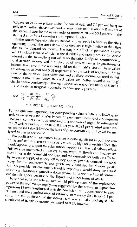
5.0 percent of mean private saving for annual data and 7.5 percent for quar-terly data Further, the annual sandard error of estimate is only 34.0 peRc'nt ofthe standard eRul far the naive model of tootnote (8 and 50.5 percent of thestandard error for a Keynesian consumption function.In the annual regression. the coefficient of y, exceeds 1.0 because the effectoperating through the stock demand for durables is large relative to the offsetdue to the demand for money. The long-run effect of permanent incomewould include induced effects on the durables and money stocks. Of specialinterest are the implied long-run values for the ratio, k, of pure consumption tototal accrued income and the ratio, o, of private saving to private-sectorincome (exclusive of the imputed yield on the durabtes stock). These valuesare estimated at 0.90 and 0.08 respectively on the basis of regression 18Y Inview of the nonlinear

transformations and auxiliary information used in theircomputations, these rather standard values are better regarded as roughchecks on the consistency of the regression than as good estimates of k and o.The short-run marginal propensity to consume is given bydc dc dye, dc' dyy20) -=--+--dy dy, dy dy1 dy,

= (1 .08) (0.15) + (0406)(085) 0.51For the quarterly regression, the corresponding value is 0.46. The lower quar-terly value reflects the smaller impact on permanent income of a one-quarterchange in current income as compared to a one-year change.

The estimates ofthis 13 weight bracket the value of 0.1 per year (0.02 5 per quarter) which wasestimated in Darby (1974) on the basis ofpure consumption. They wilt be ana-lyzed further in section IV.

The coefficient of real money balances is quite significant in both the eco-nomic and statisticalsenses. Its value is much too high for a wealth effect. Thiswould appear to support the substitution hypothesis of the real balance effect.This may be interpreted in two equivalent ways: (1) Bonds and durahies aresubstitutes in the household portfolio, and the demands for both are affectedby an excess supply of money. (2) Money supply, given its demand, is a goodproxy for the unobservable

real yields on substitutes for durable goods.Another possibly complementary liquidity hypothesis would stress the criticalrole of cash balances in providing down payments for the purchase of consum-ers' durable goods because of the illiquidity of other forms of assets.To see whether the interest rate would pick up most of the explanatorypower of the real money supplyas suggested by the Keynesian approachregression 18 was re-estimated with the coefficient of m, constrained to zero.Not only did the standard error of estimate increase by $0.9 billion (45 per-cent), but the coefficient of the interest rate was virtually unchanged. Thecoefficient of transitory income increased to 0.57, however.

b54Michael R. Darby

F:

The negative coefficient on the real durables stock is significantly larger thanthe yield on the stock. This indicates that both the direct substitution of theyield on durables for nondurable goods and services and the indirect adjust-ment of the durables stock affect consumer expenditures. Abnormally highdurables sales during a boom imply a period of abnormally low durables saleslater, while low sales during a recession imply high sales later.

The coefficient of the relative price of durable goods is insignificant and ofthe wrong sign. Although not surprising .given that about half of behaviorallydefined durable goods are represented in the denominatorthis result is dis-appointing. An unsuccessful attempt was made to estimate durahies stock andprice series inclusive of clothing and shoes. Although the relative price coeffi-cient became negative, insurmountable difficulties in estimating the initialstock and depreciation resulted in a slight deterioration in the standard error.Even were a definitionally 'pure" estimate available, there would be two otherfactors making for an insignificant, or even perversely signed, coefficient for therelative price of durables: (1) The behavior of the relative price of durables isdominated by a downward trend over the postwar period. This is probably dueto relatively rapid quality improvements in durables which mask the real pricechanges and bias the coefficient toward zero. (2) If, contrary to the usualmacroeconomic assumption, the supply curve of durable goods is not infinitelyelastic at a given price, the relative price coefficient would reflect the inter-action of demand and supply effects and be of indeterminant sign.

The nominal interest rate coefficient is slightly positive. This indicates thatthe positive effect (from decreasing the demand for money) slightly outweighsthe negative one (from decreasing the demand for durable stock). Since no at-tempt was made to adjust for expected inflation, the nominal interest ratewould not be expected to have much effect on the durables stock demand. Itis perhaps surprising then, if money demand is significantly interest-elastic, thatthe interest rate coefficient is so low.

The early part of the period, say from 1947 through 1953.. appeared suspectfor four possible reasons: (1) the constraint on durables goods purchases dur-ing World War II, (2) possible inaccuracies in the starting benchmarks for per-manent income and the durables stock, (3) the effect on the demand for

money prior to 1951-1953 of pegged interest rates on government bonds., and

(4) the Korean War and associated price controls. The equations were re-estimated for 19 54-1 973, but there was no hint of a structural change or evena significant change in any of the coefficients.2° So the entire period is retained

for the statistical analysis.

Disaggregation into Consumption and Durables Investment Equations

To illustrate the value of the integrated consumer expenditure function ap-proach, the underlying consumption function (5) arid consumers' durables in-

The Consumer Expenditure Function 65.5

TA

BLE

1D

isag

greg

atio

n of

the

Con

sum

erE

xpen

ditu

re F

uti

Usi

ng E

stim

ated

Pur

eC

onsu

mpt

ion

and

Hou

seho

ldD

urab

les

Inve

stm

ent

Reg

r.N

o. 1

Dep

.F

requ

ency

of

Var

.O

bser

vatio

nC

onst

ant

Reg

ress

ion

Coe

ffici

ents

for

(adj

.)D

.W.

/S

EE

ye1

0_)r

'Th

Ann

ual

0.88

0

2A

nnua

l(4

1 8.

2).1

54.

53.9

982

0.28

3A

nnua

l

-44.

4(-

1.08

)-ii

o.o

0.97

6(2

1.4)

0.21

9(5

.22)

0.20

8(2

.14)

-0.1

90(-

3.78

)-2

.95

(-0,

12)

3.51

(3.6

9).1

51.

4099

9820

6

4Q

uart

erly

(-2,

08)

0.10

6(1

.80)

0.19

8(3

,66)

0.49

8(3

.98)

-0.0

90(-

-1.3

9)33

,7(1

,02)

-2.1

2(-

1,73

)15

1 81

.935

82.

01

5

0.87

6(6

1 9.

3).0

11

5399

670.

06

6

Qua

rter

ly

Qua

rter

ly

-7.6

5(-

1.36

)-2

1.1

0.79

4(3

8.0)

0.26

5('1

1.7)

0.07

8(4

.96)

0.00

8(1

.32)

-1.2

4(-

0.35

)0.

857

(6.0

1).0

104

7.9

997

1.05

(-3.

01)

0.10

4(4

.00)

0.19

3(6

.78)

0.11

2(5

.70)

-0.0

25(-

3.32

)42

4(0

96)

-0.4

88(-

2.74

).0

105

989

510.

95N

Ull

Fig

ures

in p

1ren

thes

e ar

eva

lues

.es

timat

es a

re fr

om e

quat

ions

18

and

19

The Consumer Expenditure Function 657

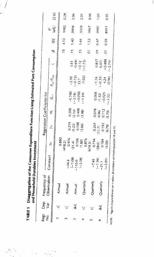
vestment function (10) were also estimated separately. F:or this purpose, theofficial delinition of durable goods was used to construct estimates (as ex-plained in "Data Definitions,' above) of pure consumption, c, and householddurables investment,

Table 1 contains the regression results. Equation 5 is estimated by regres-sions 1 and 4 for annual and quarterly data respectively. The previous indirectcalculation of k as 0.90 corresponds well to the direct estimate of 0.88. Since itwas argued that a pure consumption estimate based on the official durablesdefinition would in fact include considerable household investment in mis-classified durables, regressions 2 and 5 apply the consumer expenditure func-tion to estimated "pure consumption." Regressions 3 and 6 apply the house-hold durables investment function (10) to estimated net investment in(officially classified) durable goods.

In comparing regressions 2 and 3, it is clear that the estimated net invest-ment contains about half of total net investment in a behavioral sense.21 Theonly significant problemnot present in the quarterly regressionsis that thecoefficient on the Tagged durables stock is larger in regression 2 than in 3. Thisapparently offsets a slightly high estimated /3 weight of current income in per-manent income, while quarterly regressions 5 and 6 display the opposite bias,owing to a low /3 weight.22 The signs of the coefficients of the relative price ofdurables are just the reverse of what would be expected, but not much can bemade of the statistically insignificant results for that variable.

In sum, the disaggregated version of the model is very much what would beguessed from its derivation and the estimates of the integrated consumer ex-penditure function. The only significant divergence between the annual andquarterly resultsautocorrelation asideis apparently due to the use of aslightly too high value of /3 in the annual regressions and a slightly too lowvalue in the quarterly regressions.

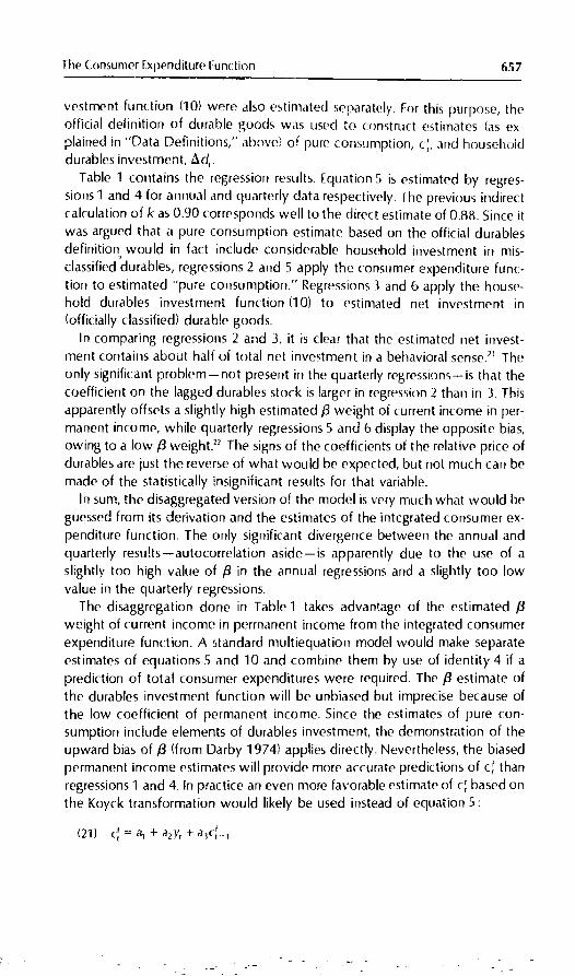
The disaggregation done in Table 1 takes advantage of the estimated /3weight of current income in permanent income from the integrated consumerexpenditure function. A standard multiequation model would make separateestimates of equations 5 and 10 and combine them by use of identity 4 if aprediction of total consumer expenditures were required. The /3 estimate ofthe durables investment function will be unbiased but imprecise because ofthe low coefficient of permanent income. Since the estimates of pure con-sumption include elements of durables investment, the demonstration of theupward bias of /3 (from Darby 1974) applies directly. Nevertheless, the biasedpermanent income estimates will provide more accurate predictions of c thanregressions 1 and 4. In practice an even more favorable estimate of c based onthe Koyck transformation would likely be used instead of equation 5:

(21) c = a1 + a2y +

Mu had R. Darhy

The square roots of the mean squared error 1 947-1 973, for the annual andquarterly Consumer expenditure functions (regression equations 1 R and 19) are1 .704 and 0.720. The corresponding ligures for the maximum likelihood esti-mates of equations 5 and 10 combined by equation 4 are 3.458 and 1.1 50. Forthe maximum likelihood estimates oi equations 21 fKoyck) and 10 combinedby equation 4, the figures are 2.635 and 0.731. The integrated Consumer ex-penditure function does niuh better than either disaggregated approach forthe annual data. But for quarterly data, the method utilizing the Koyck trarisfor-mation does nearly as well. The quarterly national income accounts data ap-Fear to spread receipts and expenditures over adjacent quarters, however; sothe Koyck transformation in this case displays a spurious accuracy.

The consumer expenditure function has been successfully estimated in thissection with no significant departures from expected signs or magnitudes ofcoefficients, The estimated coefficients are internally consistent. The disaggre-gated estimates are consistent with the original hypothesis that all coefficientsother than permanent income enter because of household investment in dur-able goods but that nearly half of durable goods in a behavioral sense are in-cluded in the official data on nondurable goods and services. As a result, disag-gregate estimates of consumer expenditures derived from separate models ofpure consumption and household durables investment compare poorly withthe estimates of the integrated consumer expenditure function.

[iv] ANALYSIS OF THREE EMPIRICAL ISSUES

The consumer expenditure function is used in this section to investigatefurthe, three empirical issues: (1) the definition of current income that best ex-plains consumer expenditures, (2) the definition of money that best explainsconsumer expenditures, and (3) the value of f3, the weight of current income inthe determination of permanent income.

The two income definitions compared are the accrual and cash receipts con-cepts.2 These two definitions reflect two basic and alternative conceptions ofconsumer behavior. The accrual concept is consistent with a view of the con-sumer as a rational decision maker constrained by total wealth The cash re-ceipts concept is sensible if consumers spend nearly all the money they re-ceive. Until recently, use of the latter concept (disposable personal income)was the standard practice. A number of studies in the last decade have movedtoward the accrual concept by adding undistribtited corporate profits (as anestimate of accrued capital gains).

There are many other income definitions which could be considered. For ex-ample Barro (1974) and Kochin (1974) have recently argued that governmentbonds may not be viewed by the private sector as net wealth. In that case an

accrual definition of income would be essentially net national product lessgovernment expenditures for goods and services pius the increase in high-powered (base) money.24 Feldstein (1974) on the other hand argues for inclu-sion of an estimate of increases in "social security wealth.' Another issue con-cerns the transfer of purchasing power to the government through inflation.This would suggest subtracting the rate of inflation times high-powered moneyand government bonds (if government bonds are included in net wealth). Inview of the high estimation costs of dealing with many alternative income defi-nitions simultaneously with the other two main empirical issues, it was decidedto compare only the basic accrual and cash receipts definitions, leaving forfurther research comparison of finer differences conditional on a particularmoney definition and 3 weight.

In section III I used the M1 (currency plus demand deposits) definition ofmoney. In this section, I compare M1 with two other money definitions thathave received considerable attention by monetary economists: M, (M1 plustime deposits at commercial banks exclusive of large negotiable certificates ofdeposit) and M3 (M2 plus savings and loan and mutual savings bank deposits).

The M2 data used are an average of the monthly data deflated by the implic-it price deflator for personal consumption expenditures. Unfortunately, FederalReserve data for M4 are available only from January 1 959 on whi!e the Fried-man and Schwartz (1970) data contain no series using the official M definition.Monthly estimates of M3 for 1947 through 1958 were made on the basis of theFriedman and Schwartz data on savings and loan and mutual savings bank tie-posits.25 The M data used in this series are averages of that monthly data de-flated by the implicit price deflator for personal consumption expenditures.

In Darby (1974), removal of the specification bias resulted in an estimatedweight of 0.1 per year in terms of an essentially pure consumption model. Inthis section I examine whether that estimate holds up in the consumer expen-diture function under alternative definitions of income and money. Were f notestimated for each combination it could bias the choice of the best combina-tion of income and money.

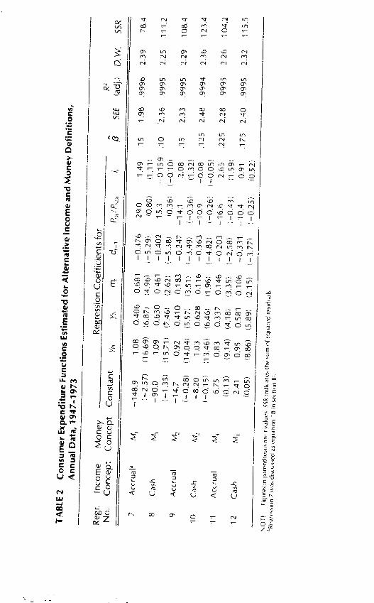
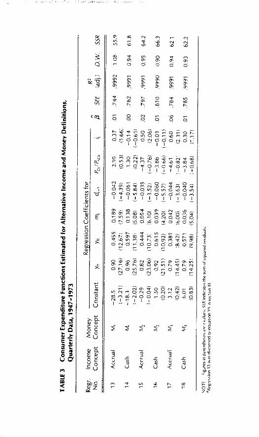
These three empirical irsues are examined simultaneously, using the regres-sions reported in tables 2 (annual data) and 3 (quarterly data). The message ofthese tables is very clear: The accrual income concept and the ftv money con-cept do much better in explanatory power (as judged by the sum of squaredresiduals or standard error of estimate) than the alternatives. Further, the f3weight of 0.1 per year previously estimated on the basis of pure consumptioncontinues to hold up in the consumer expenditure function.

Consider first the definition of income: For each money definition and forboth annual and quarterly data, the accrual definition of income does betterthan the cash receipts definition.7 SSR for the best cash receipts definition re-gression exceeds that of the corresponding accrual definition by 41 .8 percentfor the annual data and 10.6 percent for the quarterly data.2 Given the success

the Consumer Expenditure Function 659

I,

TA

BLE

2C

onsu

mer

Exp

endi

ture

Fun

ctio

nsE

stim

ated

for

Alte

rnat

ive

inco

me

and

Mon

ey D

efin

ition

s,A

nnua

l Dat

a, 1

947-

1973

Reg

r.N

o.In

com

eM

oney

Con

cept

Con

cept

Feg

ress

ion

Coe

ffici

ents

for

/3S

EE

R

(adj

.)O

W.

SS

RC

onst

ant

y,y,

rnI/P

)7 8

Acc

rual

Cas

h

M1

M.

-148

.9(-

2.57

)1.

08(1

6.69

)0.

406

(6.8

7)0.

681

(4.9

6)-0

.376

-5.2

9)29

.0(0

.80)

1.49

(1.1

1)15

1.98

.999

62.

3978

4

9A

ccru

al

-90,

0(-

1.35

)1.

09(1

5.71

)0.

630

(.46

)0.

461

(2.6

2)-0

.402

(-5.

38)

15.3

(0,3

6)-0

.159

-0 'I

D)

.10

2.36

9995

2.25

111.

2

10C

h-1

4.7

(-0.

28)

0.92

(14.

04)

0.41

0(5

.57)

0.13

3(3

.51)

-0.2

47(-

3,49

)-1

4,1

(-0.

36)

2.08

(1 3

2).1

52.

3399

952.

2910

8.4

11A

ccru

al

M.

-8.2

0(-

0,15

)1.

03(1

3.46

)0.

628

(6.4

6)0.

116

(1.9

6)-0

.363

(-4.

82)

-10.

9(-

0.26

)-0

.08

(-0,

05)

.125

2.48

.999

42.

3612

3.4

12C

ash

6.75

(0.1

3)0.

83(9

.14)

0.33

7(4

.18)

0.14

6(3

,35)

-0.2

03(-

2.58

)-1

6.6

-0,4

.3)

2.65

(1.5

9).2

252.

28.9

995

2.26

104.

2

2.41

(0.0

5)0.

95(8

.86)

0.58

1(5

.89)

0.10

6(2

.15)

-0.3

31(-

3,77

)-'(

0.4

(-0,

25)

0.91

(052

).1

752.

4099

952

3211

5.5

N(.

)TF

Fig

ure'

. in

parr

nth(

s(".

r'va

(ut-

.SS

R n

dl(

us th

e um

quar

ed IC

SiIi

UI(

S7

Wa'

. dis

cuss

ed a

s 'q

uatio

n 18

inS

ectio

n iii

NO

TE

:F

igur

es in

psr

ehe

ses

are

.SR

indi

cate

s th

e su

m o

squ

ared

res

idua

ls.

aReg

reIo

n 13

was

dis

cuss

ed a

s eq

uatio

n 19

in w

ttion

III,

TA

BLE

3C

onsu

mer

Exp

endi

ture

Fun

ctio

ns E

stim

ated

for

Alte

rnat

ive

Inco

me

and

Mon

ey D

efin

ition

s,Q

uart

erly

Dat

a, 1

947-

1973

Reg

r.N

o.In

com

eC

once

ptM

oney

Con

cept

Reg

ress

ion

Coe

ffici

ents

for

/3S

EE

R2

(adj

.)i).

W.

SS

RC

onst

ant

y,m

,c

P0/

PJJ

(1

13A

ccru

alM

1-2

8.5

0.90

0.45

50.

189

-0.0

422.

950.

37.0

1.7

44.9

992

1.08

55.9

(-3.

21)

(27.

16)

(12.

67)

(7.5

9)(-

4.39

)(0

.53)

(1.6

6)14

Cas

h-1

8.3

0.96

0.59

70.

138

-0.0

611.

30-0

.14

.00

.782

.999

10.

9461

.8(-

2.02

)(2

5.76

)(1

1.38

)(5

.08)

(-5.

84)

0.22

)(-

0.61

)15

Acc

rual

-0.2

90.

820.

444

0.05

4-0

.035

--4.

370.

50.0

2.7

9799

910.

9564

.2(-

0.04

)(2

3.06

)(1

0.73

)(6

.10)

(-3.

52)

(-07

6)(2

.06)

16C

ash

1,50

0.92

0.61

50.

039

-0.0

60-3

.86

--0.

03.0

1.8

10.9

990

0.90

66.3

(0.2

0)(2

1.51

)(1

0.92

)(4

.20)

(-5.

57)

(-0.

66)

(-0.

11)

17A

ccru

al3.

120.

790.

381

0.04

2-0

.044

-4,6

10.

60.0

6.7

84.9

991

0.94

62.1

(0.4

2)(1

4.45

)(8

.42)

(6.0

0)(-

3.63

)-0

.82

(2.3

1)18

Cas

hM

36.

010.

790.

571

0.03

6-0

.040

-3.8

40.

30.0

1.7

85.9

991

0.93

62.2

(0.8

3)(1

4.25

)(9

.98)

(5.0

4)(-

3.54

)(-

0.68

)(1

.17)

of the model, which posits rational (onsum('rs laced with a wealth constraintit would have been disconcerting to discover that the a cru.il (Jefir litiuri of in-(Orne did not do considerably l)etter Ihall the cash receipts (lPfIIliLiOil.

As to tIw empirical definition of money, the results are similar. For either deli-flition of income, the M1 definition does better than either M, or M. Comparedwith the best M1 estimate, SR for the best alternative, M, is 132.9 per(enthigher for annual data and 111 percent higher for quarterly data. The cot16-dents of real money balances Would be expected to decline in moving fromM1 to M, to M1 (because of the increasing absolute magnitudes). However, thestandard errors decline less rapidly (hence the t values fall), suggesting that kand M1 ale properly interpreted as proxies for M,

. In addition, M3 does a bitbetter than M2 suggesting that onsuniers find bank and nonbank time de-posits much better substitutes for each other than they find all kinds of timedeposits for M1.

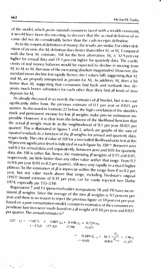
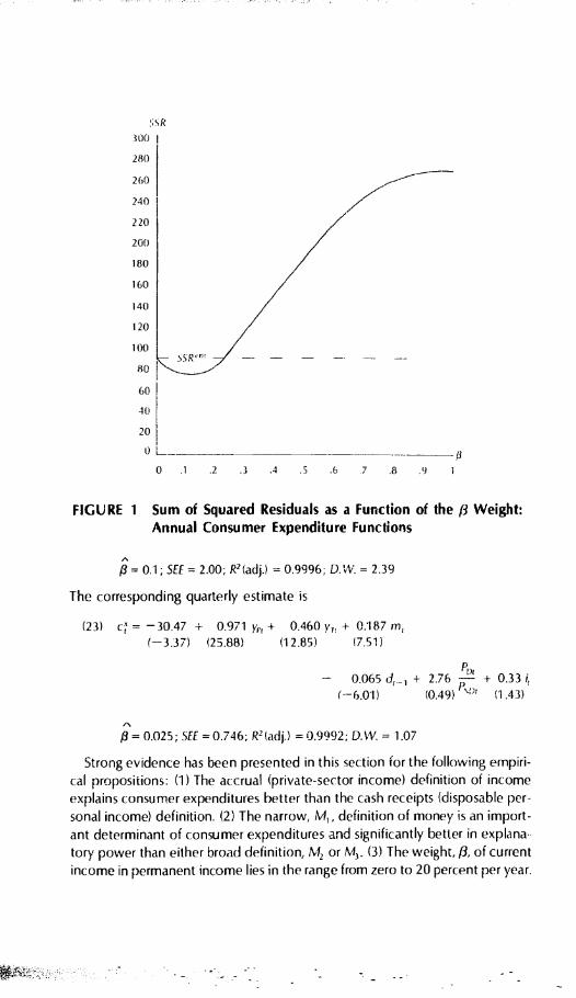
As already discussed in sect ion Ill, the estirliates of /3 bracket, but iii no casesignifi( antly differ from the previous estimate of (II per year or 0.025 perqiarter. As discussed ill footnote 22 below, the high correlation of the durablesstock and permanent income for low /3 weights make precise estimation im-possible. However, it is clear from the behavior of the likelihood function thatthe actual 13 weight must lie in the neighborhood of 0.1 P°' year (0.025 P(ltlarter). This is illustrated in hgures 1 and 2, which are graphs of the sum ofsquared residuals as a function of the /3 weights for annual and quarterly data,respectively. The ritual value of SSR for a two-tailed likelihood ratio test at the90 percent significance level is indicated in each figure by SSR''. Between zeroand 0.2 for annual data arid, equivalently between zero and 0.05 for quarterlydata, the SSR is rather flat; hence, the minimizing /3 weights of 0.15 and 0.01,respectively, are little better than any other value within that range. From 0.2to 0.6 per year (0.05 to 0.2 per qUarter), SSR rises very rapidly to a much higherplateau. So the estimation of /3 is imprecise within the range from 0 to 0.2 peryear, hut any value much above that range, including Friedman's original(1957) biased estimate of 0.35 per year, can be easily rejected (see Darby1974, especially pp. 233-234).

Regressions 7 and 1 3 (presented earlier as equations 18 and 19) have incon-sistent /3 weights. Since the average of the two [3 weights is 9.5 percent peryear and there is no reason to reject the previous figure of 10 trctnt per yearbased on a pure consumption model, consistent estimates of the consi,riir'r ex-penditure function Were mach' based on a /3 weight of 0.10 per year arid 0.025per quarter. The annual estimate is

(22) ;= - 147.5 + 1.005 + 0.446 y, + 0.729 rn(-2 52) (17.42) (7.98) (5.07)

I,- 0.2891

30.1 -- -t- .96 I,4.601 (0.83) .47)

662Mi hael R. 1)arhy

I

L

S5 R

300

280

260

240

220

200

160

160

140

120

1 00

80

60

40

20

0

-

0 .1 .2 .4 .5 .6 7 .8 .9 1

FIGURE 1 Sum of Squared Residuals as a Function of the /3 Weight:Annual Consumer Expenditure Functions

13 0.1; SEE = 2.00; R2(adj.) = 0.9996; D.W. = 2.39

The corresponding quarterly estimate is

(23) c' = 30.47 + 0.971 yp + 0.460 y + 0.187 rn(-3.37) (25.88) (12.85) (7.51)

- 0.065 cJ._ + 2.76 - + 0.33(--6.01) (0.49)

P\)(1.43)

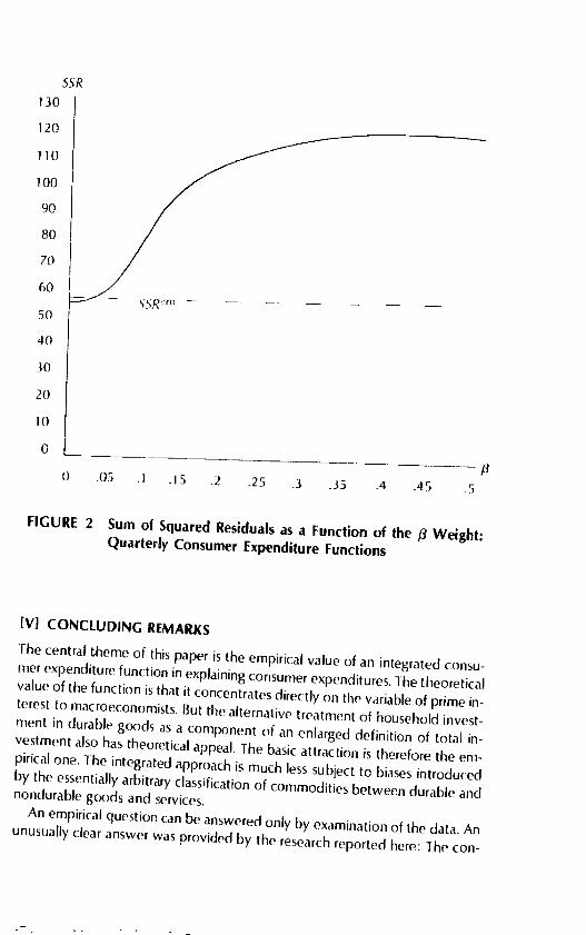
f3= 0.025; SEE = 0.746; R2(adj.) = 0.9992; D.W = 1.07

Strong evidence has been presented in this section for the following empiri-cal propositions: (1) The accrual (private-sector income) definition of incomeexplains consumer expenditures better than the cash receipts (disposable per-sonal income) definition. (2) The narrow, M, definition of money is an import-ant determinant of consumer expenditures and significantly better in explanatory power than either broad definition, M2 or M3. (3) The weight, /3, of currentincome in permanent income lies in the range from zero to 20 percent per year.

)

SSR

130

120

110

100

90

80

70

60

50

40

30

20

10

0

-

0 .05 .1 .15 .2 .25 .3 .35 .4 .45 .5

FIGURE 2 Sum of Squared Residuals as a Function of the f3 Weight;Quarterly Consumer Expenditure Functions

[VJ CONCLUDING REMARKS

The central theme of this paper is the empirical value of an integrated consu-mer expenditure function in explaining consumer expenditures The theoreticalvalue of the function is that it concentrates directly on the variable of prime in-terest to macroeconomists But the alternative treatment of household invest-ment in durable goods as a component of an enlarged definition of total in-vestment also has theoretical appeal. The basic attraction is therefore the em-pirical one. The integrated approach is much less subject to biases introducedby the essentially arbitrary classification of commodities between durable andnondurable goods and services.An empirical question can be answered only by examination of the data. Anunusually clear answer was provided by the research reported here: The con-

surner expenditure function explains the data well and significantly better thanthe multiequation, pure consumption-household investment approach. Thereason for this superior performance is that the official data on durable goodsexpenditures include only about half of total durables expenditures as definedbehaviorally.

The data also provided strong evidence that (1) an accrual (private-sector)definition of income better explains consumer expenditures than a cash re-ceipts (disposable) personal income definition; (2) the narrow, M, definitionsimilarly does better than either M2 or M; and (3) the /3 weight of current in-come in the formation of permanent income lies somewhere in the range fromzero to about 20 percent per annum. While there is no a priori presumptionabout the best money definition, the results based on the income definitionand the /3 weight reinforce the basic conception underlying the modelthatconsumers are rational decision makers constrained by total (human and non-human) wealth as estimated by permanent income. The rationality of corisu-rners would certainly be questionable if they responded to cash receipts ratherthan accrued income. A /3 weight of about 10 percent per annum, which is theestimated real yield on total wealth, is preferred to the higher weights esti-mated in many previous studies.'

The empirical advantages of an integrated consumer expenditure functionseem clear. Future research might be directed at substituting a life-cycle model

for the permanent income explanation of pure consumption to conipare theirexplanatory powers. Other areas for possible improvement would be eitherthe generalized stock adjustment hypothesis (6) or the underlying stock de-mand functions (7) and (9). A somewhat different line of research would utilizeie consumer expenditure function to examine finer definitions of accrued in-

come adjusted for increases in government debt, in social security wealth, or

the inflationary tax on base money and possibly government debt.

DATA APPENDIX

Several data series of general applicability were estimated in the course of this

project. In order to make them available for future research by others in this

and other areas, the most important are reprodLiced here with instructions forupdating as revised data become available.

Table A-i contains annual data for nominal and real private-sector income,the current and permanent (real) income on the accrued definition, the real

durables stock, and the nominal M money supply. Table A-2 contains quar-terly data for the same series. Table A-3 contains the monthly nominal M3 datathrough 1 959, when they tie in with the Federal Reserve Board's publisheddata.

The Consumer Expenditure Function 665

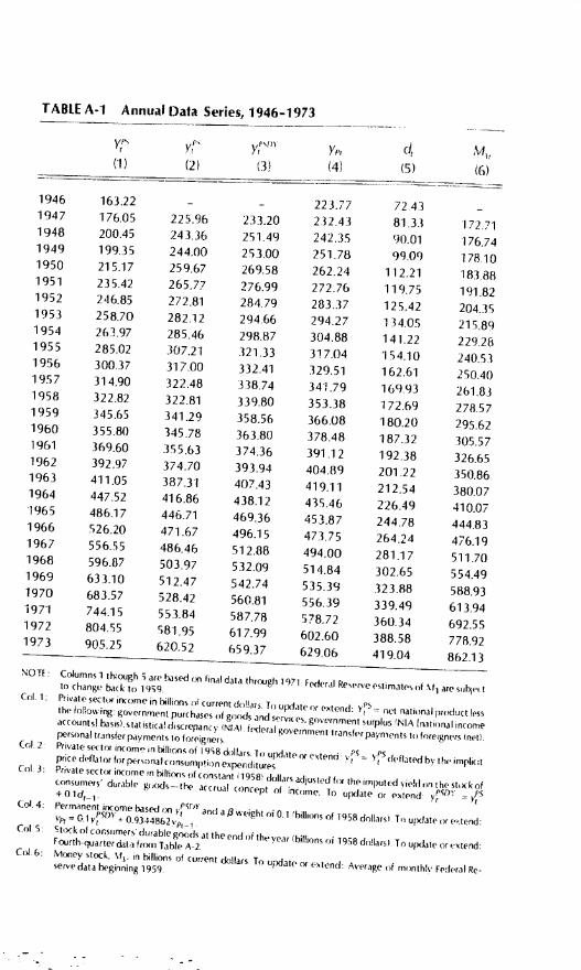
TABLE A-i Annua' Data Series, 1946-1973

1946 163.22 - - 223.77 7243 -1947 176.05 225% 233.20 232.43 81.33 172 711948 200.45 243.36 251.49 242.35 90.01 176.741949 19935 244.00 253.00 251.78 99.09 178101950 21 517 259.67 269.58 26224 112.21 183881951 235.42 265.77 276.99 272.76 119.75 191 821952 246.85 272.81 284.79 283.37 125.42 204.351953 258.70 282.12 294.66 294.27 134.05 215 891954 263.97 285.46 298.87 304.88 141.22 229281955 285.02 307.21 321.33 317.04 154.10 240511956 300.37 317.00 332.41 329.51 162.61 250401957 314.90 322.48 338.74 341.79 169.93 261 831958 322.82 322.81 339.80 353.38 172.69 278571959 345.65 341.29 358.56 366.08 18020 295621960 355.80 345.78 363.80 378.48 187.32 305571961 369.60 355.63 374.36 391.12 192 38 326.651962 392.97 374.70 393.94 404.89 201 22 350.861963 411.05 387.31 407.43 419.11 212.54 380.071964 447.52 416.86 438.12 435.46 226.49 410.071965 486.17 446.71 469.36 453.87 24478 444.831966 526.20 471.67 496.15 473.75 264.24 476.191967 556.55 486.46 512.88 494.00 281.17 511.701968 596.87 503.97 532.09 514.84 302.65 554.491969 633.10 512.47 542.74 535.39 323.88 588.931970 683.57 528.42 560.81 556.39 3394g 613941971 744.15 553.84 587.73 578.72 360.34 692.551972 304.55 581.95 617.99 602.60 388.58 778921973 905.25 620.52 659.37 629.06 419.04 862.13

NOTE. Cumns 1 thgh are based final data throogh 1971 FederalReserve estimates of Sf are sIihi. Ito change back to 1959

Cot 1- P'ivate setx income in fIIis of current do!!as To Uate or extend- Ynet national product lessthe folioss i government purchases of goods and

sCices. gneernment surplus NIA Inaijonal incomeaccountsl basis),statisticaf dcrepancy (NAI frderatgovernrntransfer payments to foreigners nellpersonal transfer payments to foreigners

(of 2 Private sect women beirooc of 1958 oollars. Ti)update orentend- v fS deflated by the impliotprice deflator for personal

consumption esperdituresCot 3- PrrvateslOr Income n ltroos of constant 1958 dc,Ilarsadjusted fix the imputed s-jeSt on the stock ofvonsuniers durable goods-tbe accrual concept of incrime. To update or estend

=± 0.1d1_1.

C 4 Permanent Income based 1PTiyand a 4 weight 010.1 hillioos of 1958 dotlarsr To update ore. tendG.ly0 + O.9344862v1

Cot 5 Stock of consumers durable goods at the end of the year 'billionsof 1958 dotlarsi To update or sstendImirtli-quarter dat-a from Table A-2.

C 6: Mcmey stock 5f, in llions of current dollars To update ni estenci...erageof monthly Federal Re-serve data beginning 1959.

Ye, cjr

(4) (5)

TABLE A-2 Quarterly Data Series, 1964:4-1973:4

(1)

',pcIf

(2) (3) (4) (5) (6)

1946:4 169.9 - - 227.17 72.43 -1947:1 170.4 223.62 230.87 229.39 74.56 169.191947:2 172.0 223.96 231.41 231.58 76.76 171.881947:3 179.3 228.99 236.67 233.88 78.89 174.061947:4 182.5 227.27 235.16 236.09 81.33 175.721948:1 190.5 234.90 243.03 238.47 83.63 176.741948:2 199.5 243.29 251.66 241.03 85.83 176.271948:3 205.1 246.22 254.80 243.63 88.02 176.961948:4 206.7 249.04 257.84 246.26 90.01 176.991949:1 201.1 244.35 253.35 248.74 91.77 177.051949:2 198.9 243.15 252.33 251,15 94.01 178.041949:3 199.8 245.76 255.16 253.60 96.48 178.341949:4 197.6 242.75 252.40 255.94 99.09 178.971950:1 209.5 257.69 267.60 258.63 101.86 180.751950:2 209.7 256.67 266.86 261.25 104.59 183.501950:3 217.3 260.24 270.70 263.93 109.11 184.871950:4 224.2 264.08 274.99 266.67 112.21 186.421951 :1 226.0 257.11 268.33 269.20 115.28 187.971951:2 234.6 265.99 277.51 271.93 117.00 190.001951:3 240.0 271.19 282.89 274.74 118.43 192.801951:4 241.1 268.78 280.63 277.46 119.75 196.501952:1 241.9 268.78 280.75 280.13 121.08 199.801952:2 242.6 269.26 281.36 282.78 122.51 202.661952:3 248.0 273.73 285.98 285.51 123.40 205.851952:4 254.9 279.50 291.84 288.33 125.42 209.081953:1 258.0 282.58 295.13 291.20 127.75 211.721953:2 260.1 284.26 297.04 294.06 129.97 214.981953:3 259.6 202.17 295.17 296.84 132.05 217.261953:4 257.1 279.46 292.66 299.51 134.05 219.601954:1 260.6 281.42 294.83 302.19 135.61 229.131954:2 261.3 282.18 295.74 304.86 137.34 225.621954:3 263.6 285.28 299.01 307.56 139.08 229.511954:4 270.4 292.96 306.86 310.42 141.22 232.871955:1 276.6 298.70 312.83 313.38 144.08 236.601955:2 283.7 306.37 320.78 316.49 147.45 239.401955:3 287.4 30936 324.11 319.64 151.00 241.871955:4 292.4 314.41 329.51 322.88 154.10 244.271956:1 293.9 313.99 329.40 326.06 156.46 246.531956:2 297.8 315.80 331.45 329.24 158.63 249.101956:3 302.3 317.21 333.07 332.41 160.50 251.501956:4 307.5 320.98 337.03 335.63 162.61 254.471957:1 311.1 321.72 337.98 338.83 164.84 257.63

p

TABLE A-2 (continued)

(1)

'P.

(2)

ySf)

(3) (4)

d,

(5) (6)

1957:2 314.2 322.92 339.40 342.0! 166.72 260.601957:3 318.0 324.16 340.83 345.18 168.37 263 .4 31957:4 316.3 321.12 33795 348.22 169.93 265.671953:1 314.4 315.66 332.65 351.09 170.72 269.601958:2 3176 317.60 334.67 353.96 171.20 276.471958:3 325.1 324,77 341.89 356.97 171.83 281.801958:4 334.2 333.20 350.38 360.14 17269 286A31959:1 339.8 337.77 355.04 363.38 174.35 290.901959:2 348.1 344,99 362.43 366.75 176.43 294.731959:3 345.3 339.86 357.50 369.95 178.60 297.871959:4 349.4 342.55 360.41 373.17 180.20 299.001960:1 354.1 346.14 364.16 37643 182.25 299.801960:2 356.9 347.52 365.74 379.68 184.26 302.071960:3 357.2 346.80 365.22 382.87 186.01 307.501960:4 355.0 342.66 361.27 385.91 187.32 312.931961:1 357.7 344.60 363.34 388.95 188.11 318.271961:2 366.0 352.94 371.75 392.15 189,24 323.971961:3 372.6 358.27 377.19 395.44 190.62 329.431961:4 382.1 366.70 385.76 398.90 192.38 334.931962:1 386.9 370.24 389.48 402.39 194.48 341.471962:2 391.6 374.02 393,47 405.93 196.48 348.331962:3 394.4 375.62 395.27 409.46 198.77 353.271962:4 399.0 378.92 398.79 413.02 201.22 360.371963:1 402.6 381.25 401.37 416.59 203.88 368.631963:2 406.7 383.68 404.07 420.17 206.60 376.501963:3

1963:4414.1 389.92 410.58 423.85 209.53 383.70420.8 394.38 415.33 427.60 212.54 391.431964:1 433.5 405.52 426.77 431.58 215.95 397.731964:2

1964:3445.7 415.38 436.97 435.75 219.61 404.83

1964:4453.2 421.97 443,93 44002 223.35 414.27

1965:1457.7 424.55 446.92 444.31 226.49 423.47

1965:21965:31965:41966:1

469.0477.0493.6505.1

433.46438.42452.84462.12

456.11

461.52

476.36486.10

448.76453.27458.0846307

231.03235.15

239.75

244.78

432.20439.50448.37459.27

1966:21966:31966:41967:1

1967:21967:31967:41968:1

513.5520.0529.6541.7544.5550.8560.7570.2579.6

465.97467.21

473.28480.23

480.58484.01

488.41492.83496.23

490.45492.23498.75506.19

507.01510.82515.69520.52524.35

46808473.06478.124832948840493.53498.69503.90509.12

250.26254.71

25.60264.24268.12

272.75276.98281,17286.27

468.13474.77

478.63

483.23

492.40

505.17

519.33529.90

538.60

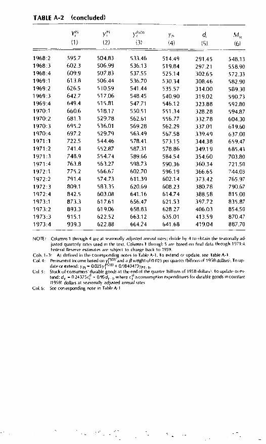
NOTE: Columns 1 through 4 are at seasonally adjusted annual rates: div,de by 4 to thtain the seasonally ad.jusled quarterly rates used in the test. Columns 1 through are based on final data through 1971:4federal Reserve estimates are subject to change back to 1959.

Cols. 1-3: As defined in the corresponding notes to Table A1. To estend or update, see Table A-i.Col. 4: Permatient income based on yfSt3t' and a /d weight of 0025 per quarter (billions of i 958 dollars). To up-

date or extend: y 0.025y'5'° + O984373Yl'L b-Col. 5: Stock of consumers' durable goods at the end of the quarter billons of 1958 dollars) To update ores-

tend: d1 = 0.24375c 0'954r- , ss' here c? is consumption espenditures for durable goods in constant1958) dollars at seasonally ad(usted annual rates.

Col.6: See cocrespondirrg note in Table A-i.

TABLE A-2 (concluded)

Ypc PS

(1) (2)

)JPSDY

I; (4)

d,

(5)

M

(6)

1968:2 595.7 504.83 533.46 514.49 291.45 548.131968:3 602.3 506.99 536.13 519.84 297.21 558.901968:4 609.9 507.83 537.55 525.14 302.65 572.331969:1 613.8 506.44 536.70 530.34 308.46 582.901969:2 626.5 510.59 541.44 535.57 314.00 589.301969:3 642.7 517.06 548.45 540.90 319.02 590.731969:4 649.4 515.81 547.71 546.12 323.88 592.801970:1 660.6 518.12 550.51 551.34 328.28 594.871970:2 681.3 529.78 562.61 556.77 332.78 604.301970:3 695.2 536.01 569.28 562.29 337.01 619.601970:4 697.2 529.79 563.49 567.58 339.49 637.001971:1 722.5 544.46 578.41 573.15 344.38 659.471971:2 741.4 552.87 587.31 578.86 349.19 685.431971:3 748.9 554.74 589.66 584.54 354.60 703.801971:4 763.8 563.27 598.73 590.36 360.34 721.501972 :1 775,2 566.67 602.70 596.19 366.65 744.03

1972:2 791.4 574.73 611.39 602.14 373.42 765.971972 :3 809.1 583.35 620.69 608.23 380.78 790.671972:4 842.5 603.08 641.16 614.74 388.58 815.00

1973:1 873.3 617.61 656.47 621.53 397.72 835.871973:2 893.3 619.06 658.83 628.27 406.03 854.50

1973:3 915.1 622.52 663.12 635.01 413.59 870.47

1973:4 939.3 622.88 664.24 641.68 419.04 887.70

I

A

TA

BLE

A-3

:E

stim

ates

of M

3 M

oney

Sto

ck,

Mon

thly

, 194

7-1

959

(sea

sona

lly a

djus

ted

mon

thly

ave

rage

s in

bill

ions

of d

olla

rs)

Feb

.M

ar.

Apr

.M

ayJu

neJu

ly

169.

017

0.2

171.

117

1.8

172.

817

3.2

176.

917

6.6

176.

317

6.1

176.

417

6.9

177.

217

7.2

177.

717

8.3

178.

217

8.3

180.

718

1.6

182.

718

3.7

184.

118

4.6

187,

918

8,5

189.

519

0.0

190.

519

1.8

199.

720

0.7

201.

720

2.6

203.

620

4,6

211.

421

3.0

214,

121

5.3

215.

521

6523

2.4

223.

522

4.1

225.

922

6.8

228.

423

7.1

237.

423

8.4

239.

624

0.2

241.

124

6,5

247.

324

8.4

248.

925

0.0

250.

625

7.6

258.

725

9,6

260.

726

1.5

262.

626

9.8

272.

127

4.4

276.

327

8,7

280.

029

0.7

292.

029

3.4

294.

829

6.0

297.

5N

OT

E=

2 m

oney

ctk

plu

s de

posi

ts a

t mut

ual s

avin

g5 b

anks

and

savi

ngs

and

loan

ass

oiat

jofls

Fed

eral

Rec

ee B

oard

dc'

fioiti

or,

Dat

a or

194

7 th

roug

h 19

58ec

est

imat

ed b

yad

ding

to 5

4t

Frim

an a

nd S

chw

artz

197

0i d

ata

on m

utua

l sav

ings

ban

k an

d sa

ving

s an

d lo

an,5

ssoy

j,flv

,de

posi

ts M

onth

ly s

avin

gs a

ndia

n da

ta w

orE

' nio

rpol

ated

twee

n an

nual

194

7194

9 an

dpu

arte

rly 1

950-

1954

t ben

chm

arks

be

Ihe

usc

o( m

utua

l sav

ings

han

kde

p'ss

its D

ata

Or

1959

are

Fed

eral

Rcc

prvc

gun'

s

S

Dec

.A

ug.

Sep

.O

ct.

Nov

.

1740

1 75

.01

75.2

1 76

.01

76.0

'177

.117

7017

7117

6.9

176.

917

8.4

1783

1786

178.

917

9418

4918

5.1

1 85

.818

6.5

186.

919

2.5

194.

119

4.8

196.

919

7.8

205.

820

7.1

2079

2092

2102

2174

217.

921

8721

9722

0422

9.6

230.

623

1.7

2330

2339

241

724

2.8

243.

724

4124

5 0

251.

325

2.6

2534

2545

255

526

3.5

264.

226

4.9

265

726

6,4

282.

028

3.4

284.

828

6628

7.9

297.

829

8.3

298.

529

9 1

2994

Yea

rJa

n.

1947

1 68

,419

4817

6719

4917

6.7

1950

179.

919

5118

7.5

1952

198.

919

5321

0,7

1954

231.

519

5523

5.3

1956

245.

819

5725

6.6

1958

266.

919

5929

0.0

The Consumer Expenditure Functjon671

MOTiS

t A rough definition of behavioral duiabilityis responsiveness to transitory income Consunierexpenditures for durable goods and for clothing and shoes are about equally responsive tochanges in transitory and permanent income, but all other expenditures are only about one-quarter as responsive to changes in transitory

compared with permanent income Thus theofficial Commerce Department definition does appear to capture goods significantly moredurable than those classifier) s nondurable goods and services (with the exception ofclothing and shoes). Given the relative magnitudes, however; the remaining durab!e ele-ments in 'nondurable goods and services" are nevertheless quite significant.In my earlier work (1972, 1975), this adjustment was neglected because of the small differ-ence from unity for quarterly data with 6 = 0.05, 1 - 056 = 0975)This adjustment, too, is small for quarterly data. Using r = 2.5 percent per quarter or 10 per-cent per year, 1 - 0.5r 0.9875 for quarterly data or 0.95 for annual dataI am assuming a constant real yield, r, here. In fact, r would vary over timeparticularlywhen the stock 01 durables is not at its long-run optimum. The observed willingness of on-sumers to use durables to absorb transitory income shocks suggests that the actual realyield variations are negligible.Darby (1974) demonstrates the interpretation of permanent income as a perpetual inven-tory of wealth.Other possible influences have been omitted either here or below in completing the specifi-cation because of the difficulty in obtaining good data and the paucity of true degrees offreedom. The empirical results that follow do not seem to have suffered muchA real interest rate is correct here. If IT is the expected inflation rate and r the marginal taxrate on interest (see Darby 1976, pp.74-75), then the a term should be a3 ji - hr/Cl - il].Carrying through to equation 10, this implies that a term lX1a3i(1 - r)hir is omittedfrom the specification. Since ir and iare positively correlated and A1a3/(1 -- TI is posi-tive, this imparts a positive bias to the estimated interest rate coefficient. The task of includ-ing an estimated inflation rate is left for future research.The coefficient of permanent incorrie will capture the effect of wealth and of secular trendsin institutions, payments technology, and so forth. The coefficient of transitory income re-flects both effects of windfalls on portfolio adjustment and of cyclical variations in transac-tions (see Darhy 1972).

unfortunately, even given the value of r, the only structural parameters that can be recov-ered from the regression coefficients are A1, A, and a2. The other ten parameters cannot beseparately identified.

Basic data series were all drawn from the NB[R data bankThis amounts to the usual ten-year-life, double-decliningbalance method. The initial valuefor December 31, 1946, was computed from Raymond Goldsmith's 1962 data as 72.43 bil-lion 1958 dollars. See Darby (1972, pp. 931-932) for details. This calculation requires that cbe measured at quarrer!y rates in order to integrate flows into stocksA theoretically more attractive definition would be to base the imputation on the averagedurables stock for the period c4 + 0.5 Ac4. This was not done because it may impartspurious correlation, particularly in the disaggregated estimation of the d1 equation.That is, private-sector income equals disposable personal income + undistributed corpor-ate profits wage accruals less disbursements + corporate inventory valuation adjustmentless other personal outlays. For computational purposes, an equivalent definition is net na-tional product less taxes net of transfers (i.e., government purchases of goods and services+ NIA [national income accountsl surplus) less government and private transfers to for-mgners less statistical discrepancy.

14 I his goissth rate is implit it iii saving plans I lii' rt't1uui'd go wili rifts anul :nitial U)= 1946 for aonninia (it,) ann) i4f,.4 for (ioarri'rlv data) were ,stuniteil h' .1 (C i('liai'nr Crrd(see Ru by 1974 Ii ir i hi .ii Is) a

Income Concepl

"iii rut (aiiiii,il iLina I) 1111332 1.

"St i ititi t(Iiiannt'ily 0,1,0 0(5 IS') 53 7') ii

iei i'ipt (innniial tim ml ii 0400 211 37 1

ash ii iipR iliiamntnly it,itml 0 01001 54 3573

IS. I his sort's is the most Inriibti'nnati il It is a'. pointed out iii tI iii!rodij lion (hat roughly hallof fwliavmi wal ly nlor able gi ii id, an' inn ttKlt'd ami tag iii inilurable goods and smrvkes. 1 hustheir pri( (5 will hi' iiiclindi'd ifl liii' (li'ilonlinitor mislead of the nunheratol. Also, the durable

ii ids pin e del lat iii is gi 'neraltv lx'! iivtd biased reIn ye to the nrindurahlcs deflatiii he-& a Lisi' ot mm 'ri rap;( I quality improvement in t hi' I' irmer

lii 1 he t val ties art' gi von in par tnt hoses The square br,u kits nd i cati I hr ii nfidrmu e inter V.1for a I)Fobability of nil ire t han 93) pert out ii inn j)Luttn) (iii the basis of I lx' swmpiit ic dnstri ho-non of lix logarithm iii the like) ihmiod funt tion. mi the annual regression, [1 0, 0(1250050.....1) 975 I (XXI was wart hid for the value that masiniiit'd (hi' likelihood friar lion Forthe quarteuiy rressnim, fl = 0, 0.01. 0.02.....(1.99, 1(X) was u'.edSee the analysis of (hi' coeffn Pills below e(Iuation it the annual oeffi( rents shiiuld beappros mat ely four times the quarterly ones es t'pt for those of and > - Only I heamount by which ext t'i'ils is iiiultiplied by 4 for y,. The coefficient , of y should beessentially tutu hanged, as the lower qujar for ly value of X, is offset by a higher vahue of yheii e, Ihi' only t'xper ted hange us due to the slightly higher quarterly value of the 1

0.Sr) rdjustnient factor.For example, a rsuve tirsl order autoregression shows a very high g2 (O the .inntial data'

= -4.72 + 1.054(-1.14) (88.47)

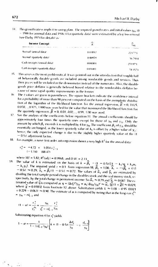
where 511 = 5.82; R2 iadj I 0.9968; and OW. = 2. 1.1.The value of k us estimated on the basis 01 k = f3 - 11 - I) SrI [(1 - A ,) + A1 a1- )sy1!. The imputed yield = 0.1. From regression 18, f3 1 08; X1 = - + '('(1- OS,) 0.29, ,/Il - 0.5,) 0.72. liii' values i)f and are estimated bydividing the total simple-perimid change in the dtirabtes stock and the real money stock, re-sper lively, by the total change in lx'rn.nent income. So 0.7') and 9 0087 The in-timated value of iS computed as n = (r!('/y,1 = n (y/y("

nlg/(1 + 0021),

where g 0.03812 1(01)) footnote 12 above. Substitution yields 1 1118 - (1 95 (0(121-t 0.229 -- 0 063) 0%. The estimate of a is computed by rn)ting that in the long-run

- rd - and

( he(1 -ir)=---=)5 y' - rd3 Y

Substituting e(luaticmn 4 to e' yields

1 1 Ai1f1 ir=----- k-s 11 -O.5d---1 - '>)

672 tsiti hai'l R. I )irby

a1

1(1

by

ro-

es-

29,

21

y,s

L

Taking d1_1/yP1 - 076,

1 - = (1/0.9241)0.90 + (095)10029) - (0.10)10.76)] = 0.92

So = 0.08.The estimates of the f3 weight of current income in permanent income were a bit closer tothe value of 0.1 per year estimated in Darby (1974). The only other noticeable-though sta-tistically insignificant-changes were generally higher (in absolute value) estimates for thecoefficients of money and the durabies stock. All these changes are consistent with the hy-pothesized shift, but the standard errors of estimate actually deteriorated slightly in thetruncated period.The coefficient of transitory income, Yri is higher in regression 3 than in 2, reflecting thelarger offset in 1 3) due to its higher money coefficient. Note that, rounding error aside, re-gressions 2 pIus 3 less 01 d.1 equal regression equation 18. Similarly, regressions 5 plus 6less 0.025 d1.1 equal regression equation 19.

I am indebted to Thomas Mayer for the observation that for low /3 weights, permanent in-come and the durables stock are closely related because of the high correlation betweentran5itory income and fluctuations in household durables investment. A high estimate of 13applies too low a weight to past transitory income and can be offset by a more negative co-efficient on the durables stock. This correlation is the probable explanation for the relativelyflat likelihood function at the low end of the f3 range, as discussed in Section IV. In regres-sions based on af3 weight of 0.1 per year (but not reproduced here), the coefIkient of d1_1is -0.092 for the c dependent variable and -0.102 for the 4 dependent variable. Con-sumer expenditure functions for J3 = 0.1 per year and 0.025 per quarter are presented insection IV.

As explained in the first part of section III, the accrual concept is private-sector income ad-justed for the yield on the durables stock, while the cash receipts concept is disposable per-

sonal income with the same adjustment. The conclusions as to the relative merits of the twoconcepts are rt affected by omission of the durables yield adjustment.To be precise, transfers to foreigners and the statistical discrepancy should also be sub-tracted.

The monthly Nt3 data for January 1947 through December 1959 are reported in the Data Ap-pendix. Monthly savings and loan deposits were interpolated between annual (1947-1949)and quarterly 11950-1954) benchmarks by the use of mutual savings bank deposits.The quarterly sums of squared residuals are biased downward by the autocorrel-stion indi-cated by the low Durbin-Watson statistics. Note that this statistic is 1.08 for the accrual def-inition and 0.94 for the cash receipts definition (regressions 13 arid 14 respectively). Onlyregressions 17 and 18 for the quarterly M3 comparison are close to a dead heat. That pre-sumably reflects some peculiarity in the data which also accounts for the unusually high /3estimate of 0.06 per quarter in regression 17.In comparing definitions such as these, the hypotheses are not strictly nested and no gener-ally acceptable significance test exists. Consider the following, however, lithe differencebetween the accrual and the cash receipts definitions were allowed to enter with a weight,.i, (to be estimated) between 0 and 1, the cash receipts definition would be nested (withthe restriction .r = 1) in the more general hypothesis that income is the sum of the accrualconcept plus i times the difference. For this model, SSR could not be greater than SSR for.t =0 (the accrual income definition). If we suppose that this upper limit on the uncon-strained sum of squares is the actual value-which is favorable to accepting the cash re-ceipts definition-the likelihood ratio test could be used. The critical value at the 5 percentsignificance level for the excess sum of squares would then be 15.3 percent for annual data

The Consumer Expenditure Function 673

and lb per out tie (10, iterlv data So oven on this apparently ginieri iiis test, the ash reeipts (h'fiflhtloii is siguitii airt Is' worse than the a rual ili'iinitroti I hi' s.iiiii' argiiriu'iit sod

criti( al values tsutilcl apply to the money (h'firiitions (I1SC(iS',i'd below211. The t va I ties are given in pa rent hoses The grea Fir than ) per) out onfideni 0 Interval fi ii (I

is 10, 0.2 'II fur annual data and It). 0.06! Ii ir q tiartoil (lat a.

29. The analvs is of this spe heat ion bias is c inta:iied in I)arhy Ji,1741 A 1(1 pen ('lit )ei Y(ai/3 Weight WaS estiiiiated there on he has is of a pore i * inSum p100 model

REFERENCES

Bairn, R. . 1 974. ''Are Government Bonds Net Wealth?'' Journal of Political I cortoui', NoveinheriDix em her

Da rhy, M. R. 1 972 '''I he A Iii n at ii in of Ira ns iti ry I n ofihi' A mi my ('15)150 fliers Assets '' Ami 'iii inIi I)Tii (liii k'c'v,es', Dx i'm lx'r.

11)74, ''TIm I'*'rmmmanent tiiii'onie Th*'iiiv ot Concuitiption\ Restatenri'ut '' Cu,irti'rli10)1(0,11 (if L((inonui( s, May.

t975 ''Postwar Ii ' Consumption. ('onciinii'r isponilitures. and Saving '' Ariiiru ,iii 1)000)0))' Revi ow, May

1976, Macro*'i onomcs lhi' TJit'ors' of tricoini', hnp/o mont, and the Pi'ice I ice) NewYork: McGraw.ililI,

Feidstcin, M. I 974. ''Six a I Sec urit v, Induced Ret irenlent, and Aregaii' Capital Ac uniulat inJournal of I'uhtical E( uncut Septem her/October.

Friedman M. 1 957. A Theoti of the ( onsurupt niii Function. Princvton, NI.: l'i inc eton UniversityPress fur National Bureau of Economic Resear(Ii,

Iric-dinaii, M, arid A. J. Schwartz, 1970. Monet,mrs' Statistics of the I frill i'd States Ri rotates,Soi,rç&', Methods, New ork: NIIER.

Culdsrnith, R. W. t9(m2. The Naionr,tI Wealth rd the United States in the Post war Period Prince-ton, NI.: Prin(etorm Universit' Press for NBER.

Km bin, F. A. 1974. ''Are Future Taxes Anticipated by Consumers l" Journal of Stones', Credit aridflanking, August.

Modigliani, F.. and R. Bruntberg. 1954. 'Utility Analysis ()nd the Consumption Funchon: An Inter-pretat 'on of Cross"Scction Data." In K. [. Kurihara, ed.. Post-Ki'yoec,ari (coflomic c NewBrunswick, NI.: Rutgers University Press.

Wactitel P. 1972. "A Model of tntrrelated Deritarid for Assets by Households '' A,tiiali of leo-noinic arid Social Mi'as iireoienit, April.

Psiit htol R. Darhy