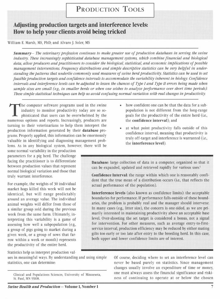
PRODUCTION TOOLS

William E. Marsh, MS,PhD; and Alvaro J. Soler, MS

Summary- The veterinary profession continues to make greater use of production databases in serving the swine

industry. These increasingly sophisticated database management systems, which combine financial and biological

data, allow producers and practitioners to consider the biologica~ statistica~ and economic implications of possible

management interventions. Frequency distributions and simple descriptive statistics can be very helpful in under-

standing the patterns that underlie commonly used measures of swine herd productivity. Statistics can be used to set

feasible production targets and confidence intervals to accommodate the variability inherent in biology. Confidence

intervals and interference levels can be adjusted to lessen the chances of Type I and Type II errors being made when

sample sizes are small (e.g., in smaller herds or when one wishes to analyze performance over short time periods).These simple statistical techniques can help us avoid confusing normal variation with real changes in productivity.

The computer software programs used in the swineindustry to monitor productivity today are so so-phisticated that users can be overwhelmed by the

numerous options and reports. Increasingly, producers areturning to their veterinarians to help them interpret theproduction information generated by their database pro-grams. Properly applied, this information can be enormouslyvaluable in identifying and diagnosing management prob-lems. As in any biological system, however, there will besome normal variability in the productionparameters for a pig herd. The challengefacing the practitioner is to differentiatebetween production values that representnormal biological variation and those thattruly warrant interference.

For example, the weights of 30 individualmarket hogs killed this week will not beidentical, but will range predictablyaround an average value. The individualanimal weights will differ from those ofa similar group sold during the previousweek from the same farm. Ultimately, in-terpreting this variability is a gam,e ofassessing how well a subpopulation (e.g.,a group of pigs going to market during agiven week, or a group of sows that far-row within a week or month) representsthe productivity of the entire herd.

how confident one can be that the data for a sub-

population is not different from the long-rangegoals for the productivity of the entire herd (Le.,the confidence interval); and

. at what point productivity falls outside of thisconfidence interval, meaning that productivity istruly off-target and interference is warranted (Le.,the interference level).

.

Statistics help us interpret production val-ues in meaningful ways. By understanding and using simplestatistics, one can determine:

Clinical and Populations Sciences, University of Minnesota,St. Paul, MN 55108.

Swine Health and Production - Volume 1,Number I

Of course, deciding where to set an interference level cannever be based purely on statistics. Since managementchanges usually involve an expenditure of time or money,one must always assess the financial significance and riski-ness of continuing to operate at or below the chosen

7

Plot thedata

Binomial variables(Yes/no, either/or)

Non-binomial variables(three or more possible values)

~Perform

sample sizecalculation

t Yes

Calculatemean andstandarddeviation

No

~~"~~"~""

Data is skewed,bi-modal, ormulti-modal.

"~(Euturearticle)

~;IFormulateconfidence

interval

Perform NormalApproximation calc.to determine inter-

ference level

tAdjust for

sample size

Decide whetheror not to actor intervene

No problem

8 Swine Health and Production - January, 1993

Collectmoredata

It..

-IrPerform ExactBinomial calc.(not in article)

the long run interference level of 10.2.Doesyour client have a problem with litter size?Is it severe enough to warrant interfereqce?Is 10.6pigs per litter a realistic target to setfor this herd? Where (given the size of thisherd and the time period you are analyz-ing) should you set the interference levelfor litter size?

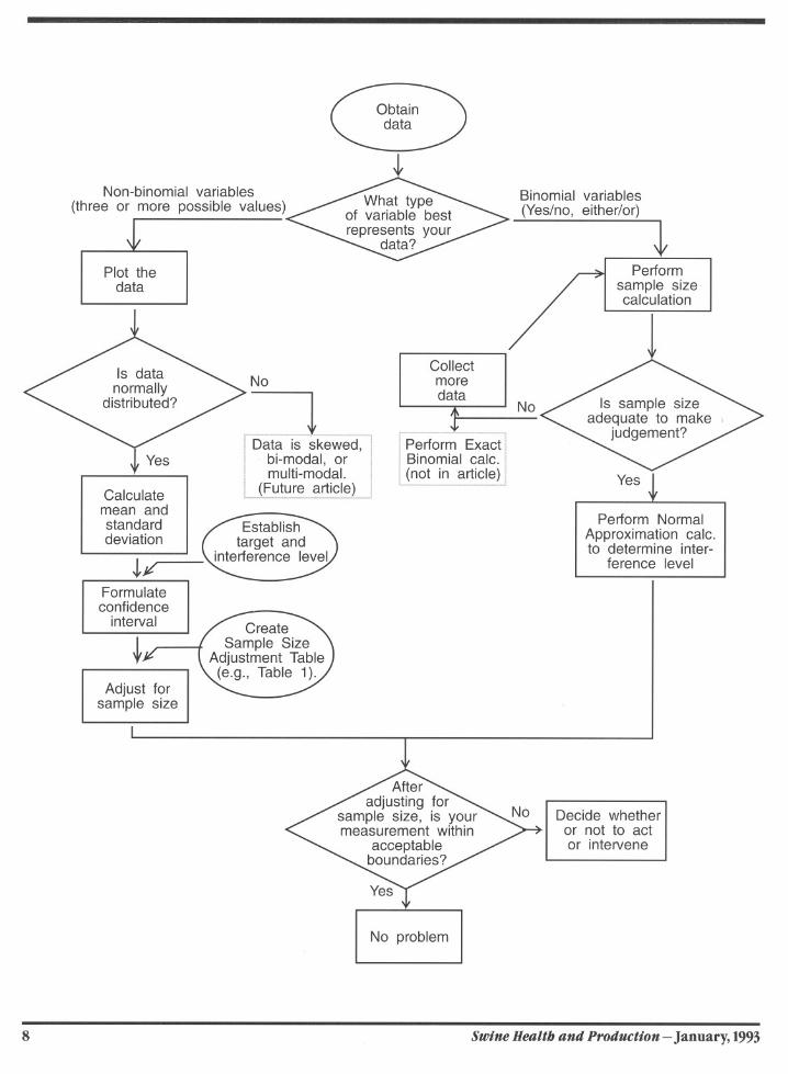
Binomial versusnonbinomial dataThe first important step in addressing thesequestions is to decide what type of data youare working with (Fig1).Litter sizedata rep-resents discrete variables that can takewhole number values over a limited range.If we were instead assessingwhether or notthe herd had a problem with farrowing rate,we would be working with binomial vari-ables, that on an individual sow basis cantake only one of two values: either the sowfarrowed, or she did not, consequent to aparticular mating event. \

Other examples of binomial variables arepreweaning mortality (a piglet lives or dies) and morbidity(the animal is diseased or healthy). Wewill discuss the pro-cedure you should use with binomial variables later in thispaper.

interference level. Because the productivity information onwhich we base management decisions is never complete andcertain, we always run the risk of "diagnosing" a manage-ment problem that doesn't really exist (a Type I error), orfailing to detect an emergingmanagement problem that trulydoes exist (a Type II error). These errorsare particularly likely when managementdecisions must be based on data from a

small sample size or short time period,because the fewer the number of obser-vations, the more difficult it is todistinguish between real differences andnormal biological variation. However,us-ing statistics to compensate can greatlyreduce the likelihood of such errors.

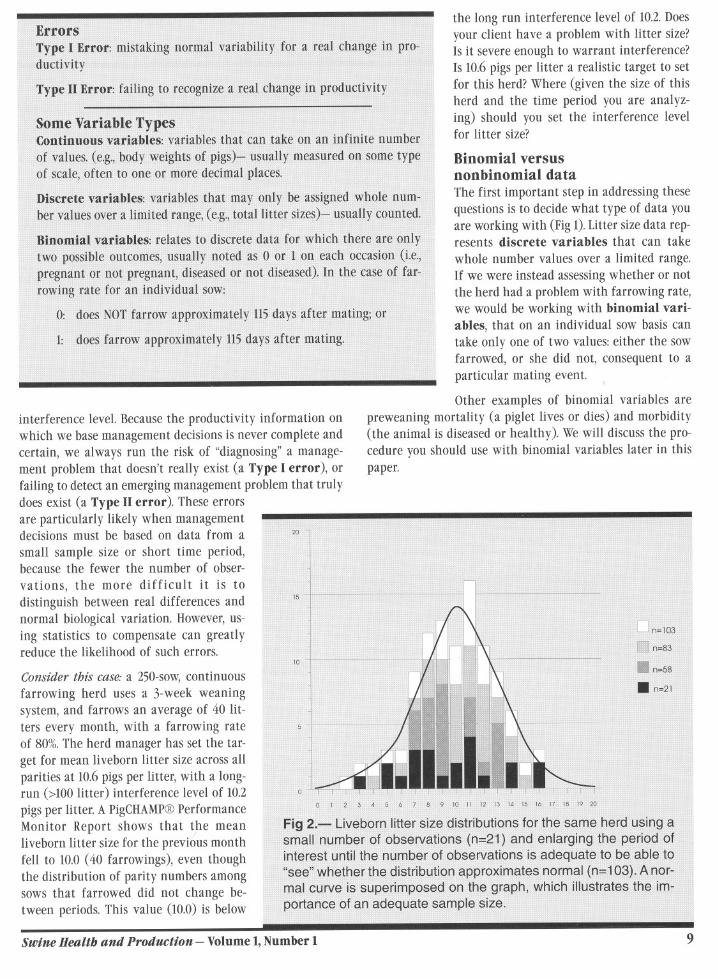
Consider this case:a 250-sow,continuousfarrowing herd uses a 3-week weaningsystem, and farrows an average of 40 lit-ters every month, with a farrowing rateof 80%.The herd manager has set the tar-get for mean liveborn litter size across allparities at 10.6pigs per litter, with a long-run (>100litter) interference level of 10.2pigs per litter. A PigCHAMP@PerformanceMonitor Report shows that the meanliveborn litter size for the previous monthfell to 10.0 (40 farrowings), even thoughthe distribution of parity numbers amongsows that farrowed did not change be-tween periods. This value (10.0) is below

Swine Health and Production - Volume1,Number1 9

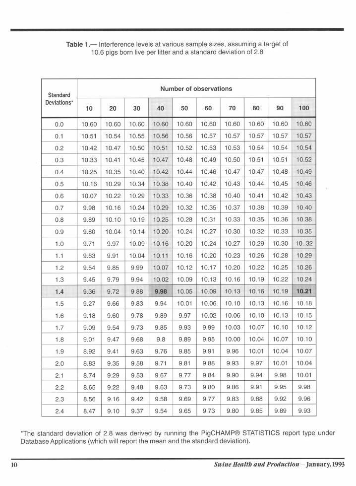
Table 1.- Interference levels at various sample sizes, assuming a target of10.6 pigs born live per litter and a standard deviation of 2.8

*The standard deviation of 2.8 was derived by running the PigCHAMP@ STATISTICS report type underDatabase Applications (which will report the mean and the standard deviation).

10 Swine Health and Production - January, 1993

Number of observationsStandard

Deviations*10 20 30 50 60 70 80 90

0.0 10.60 10.60 10.60 10.60 10.60 10.60 10.60 10.60

0.1 10.51 10.54 10.55 10.56 10.57 10.57 10.57 10.57

0.2 10.42 10.47 10.50 10.52 10.53 10.53 10.54 10.54

0.3 10.33 10.41 10.45 10.48 10.49 10.50 10.51 10.51

0.4 10.25 10.35 10.40 10.44 10.46 10.47 10.47 10.48

0.5 10.16 10.29 10.34 10.40 10.42 10.43 10.44 10.45

0.6 10.07 10.22 10.29 10.36 10.38 10.40 10.41 10.42

0.7 9.98 10.16 10.24 10.32 10.35 10.37 10.38 10.39

0.8 9.89 10.10 10.19 10.28 10.31 10.33 10.35 10.36

0.9 9.80 10.04 10.14 10.24 10.27 10.30 10.32 10.33

1.0 9.71 9.97 10.09 10.20 10.24 10.27 10.29 10.30

1.1 9.63 9.91 10.04 10.16 10.20 10.23 10.26 10.28

1.2 9.54 9.85 9.99 10.12 10.17 10.20 10.22 10.25

1.3 9.45 9.79 9.94 10.09 10.13 10.16 10.19 10.22

1.5 9.27 9.66 9.83 9.94 10.01 10.06 10.10 10.13 10.16 10.18

1.6 9.18 9.60 9.78 9.89 9.97 10.02 10.06 10.10 10.13 10.15

1.7 9.09 9.54 9.73 9.85 9.93 9.99 10.03 10.07 10.10 10.12

1.8 9.01 9.47 9.68 9.8 9.89 9.95 10.00 10.04 10.07 10.10

1.9 8.92 9.41 9.63 9.76 9.85 9.91 9.96 10.01 10.04 10.07

2.0 8.83 9.35 9.58 9.71 9.81 9.88 9.93 9.97 10.01 10.04

2.1 8.74 9.29 9.53 9.67 9.77 9.84 9.90 9.94 9.98 10.01

2.2 8.65 9.22 9.48 9.63 9.73 9.80 9.86 9.91 9.95 9.98

2.3 8.56 9.16 9.42 9.58 9.69 9.77 9.83 9.88 9.92 9.96

2.4 8.47 9.10 9.37 9.54 9.65 9.73 9.80 9.85 9.89 9.93

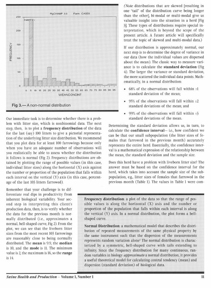
Our immediate task is to determine whether there is a prob-lem with litter size, which is nonbinomial data. The nextstep, then, is to plot a frequency distribution of the datafor the last (say) 100 litters to give a pictorial representa-tion of the underlying litter sizedistribution. Werecommendthat you plot data for at least 100 farrowings because onlywhen you have an adequate number of observations willyou realistically be able to assess whether the distributionit follows is normal (Fig 2). Frequency distributions are ob-tained by plotting the range of possible values (in this case,individual litter sizes) along the horizontal (X) axis againstthe number or proportion of the population that falls withineach interval on the vertical (Y) axis (in this case, percent-age of the last 103litters farrowed).

Remember that your challenge is to dif-ferentiate real dips in productivity frominherent biological variability. Your sec-ond step in interpreting this client'sproduction data, then, is to verify whetherthe data for the previous month is nor-mally distributed (Le., approximates anormal, bell-shaped curve,Fig2).From theplot, we can see that the liveborn littersizes from the most recent 103farrowingsare reasonably close to being normallydistributed. The mean is 9.9, the medianis 10, and the mode is 11.The minimumvalue is 2,the maximum is 16,so the rangeis 14.

(Note: distributions that are skewed [resulting inone "tail" of the distribution curve being longerthan the other], bi-modal or multi-modal give usvaluable insight into the situation in a herd [Fig3].These types of distributions require special in-terpretation, which is beyond the scope of thepresent article. A future article will specificallytreat the topic of skewed and multi-modal data.)

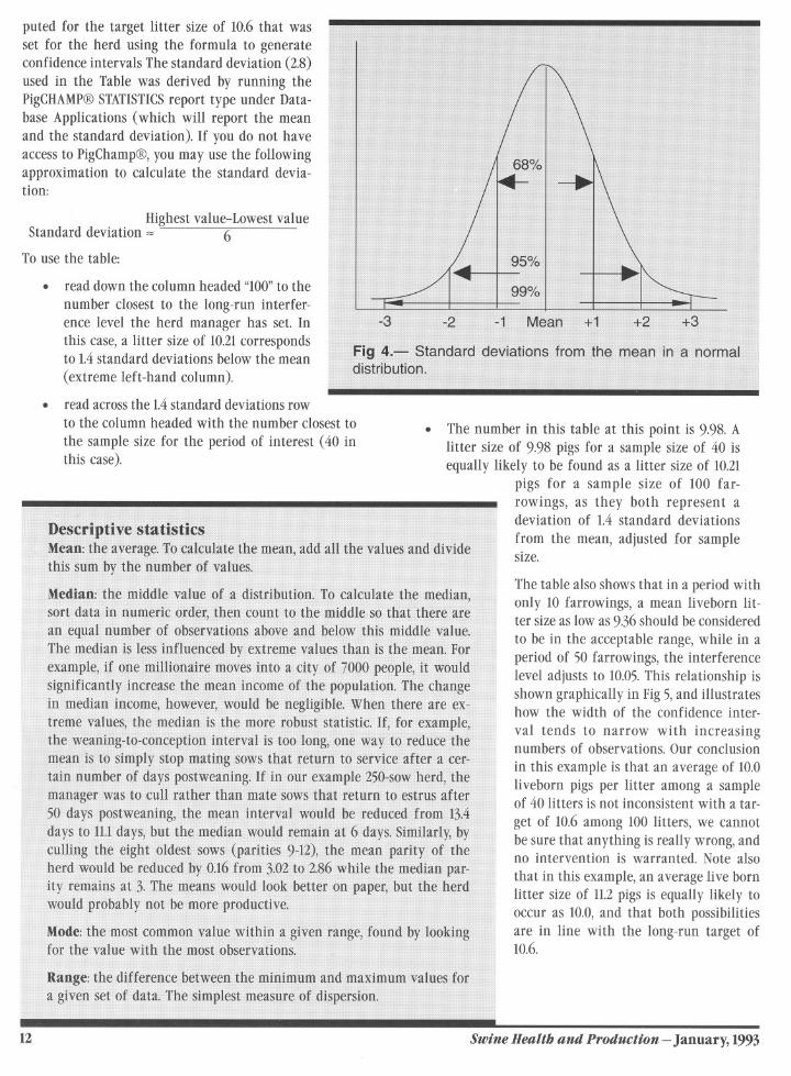
If our distribution is approximately normal, ournext step is to determine the degree of variance inour data (how the individual values are dispersedabout the mean). The classic way to measure vari-ance is to calculate the standard deviation (Fig4). The larger the variance or standard deviation,the more scattered the individual data points. Math-ematically, in a normal distribution:. 68%of the observations will fall within :tl

standard deviation of the mean;

. 95%of the observations will fall within :t2standard deviations of the mean; and

. 99% of the observations will fall within :t3standard deviations of the mean.

Determining the standard deviation allows us, in turn, tocalculate the confidence interval- Le.,how confident wecan be that our small subpopulation (the litter sizes of fe-males that farrowed in the previous month) accuratelyrepresents the entire herd. Essentially, the confidence inter-val is a mathematical expression of the relationship betweenthe mean, the standard deviation and the sample size.

Doesthis herd have a problem with liveborn litter size?Theanswer must be based on the confidence interval for the

herd, which takes into account the sample size of the sub-population, e.g.,litter sizes of females that farrowed in theprevious month (Table 1).The values in Table 1 were com-

Swine Health and Production - Volume 1,Number 1 11

puted for the target litter size of 10.6 that wasset for the herd using the formula to generateconfidence intervals The standard deviation (2.8)used in the Table was derived by running thePigCHAMP@STATISTICSreport type under Data-base Applications (which will report the meanand the standard deviation). If you do not haveaccess to PigChamp@,you may use the followingapproximation to calculate the standard devia-tion:

Highest value-Lowest valueStandard deviation = 6

To use the table:

. read down the column headed "100"to the

number closest to the long-run interfer-ence level the herd manager has set. Inthis case, a litter size of 10.21correspondsto 1.4standard deviations below the mean

(extreme left-hand column).

read acrossthe 1.4standard deviations rowto the column headed with the number closest to

the sample size for the period of interest (40 inthis case).

.The number in this table at this point is 9.98. Alitter size of 9.98 pigs for a sample size of 40 isequally likely to be found as a litter size of 10.21

pigs for a sample size of 100 far-rowings, as they both represent adeviation of 1.4 standard deviations

from the mean, adjusted for samplesize.

.

12

The table also shows that in a period withonly 10 farrowings, a mean liveborn lit-ter sizeas low as 9.36should be consideredto be in the acceptable range, while in aperiod of 50 farrowings, the interferencelevel adjusts to 10.05.This relationship isshown graphically in Fig5,and illustrateshow the width of the confidence inter-

val tends to narrow with increasingnumbers of observations. Our conclusion

in this example is that an average of 10.0liveborn pigs per litter among a sampleof 40 litters is not inconsistent with a tar-

get of 10.6among 100 litters, we cannotbe sure that anything is really wrong, andno intervention is warranted. Note also

that in this example, an average live bornlitter size of 11.2pigs is equally likely tooccur as 10.0,and that both possibilitiesare in line with the long-run target of10.6.

Swine Health and Production - January,1993

Interpreting binomial variablesWe would apply the same statistical principles ifour task were to investigate a problem with far-rowing rate (Le. a binomial variable). Unlike thenormal distribution, the binomial distribution isnot usually described by a mean and standard de-viation. Rather, it is based on a mathematicalexpression that considers the probability of a num-ber of successes (farrowings) occurring out of anumber of trials (services).

Consider this case:Let's look at the same herd and

determine whether it has a problem with farrow-ing rate (based on 40 litters per month). Tocalculatethe farrowing rate, we must look back 115days andsee how many females were mated during a corre-sponding I-month period. Most managers breedmore than they expect to farrow because the far-rowing rate is never 100%.For example,if 50femaleswere bred during the corresponding I-month pe-riod, and 40 farrowings resulted from thosematings, the farrowing rate is calculated as:

40+ 50= 0.8,or 80%

Howdo we calculate confidence intervals for pro-ductivity parameters that follow a binomial distribution?First,we must determine whether we have an adequate num-ber of observations to draw safe conclusions (Fig 1).We doso by performing the following "sample size" calculation:

Target Ratex(1-Target Rate)xsample size must be ;:::5.

In the case of an 80%Target Farrowing Rate (TFR}

(0.8x(1-0.8)xminimum sample size)=5(0.8xO.2)xminimumsample size=5Minimum sample size = 5/0.16Minimumsamplesize= 31.25

An adequate sample size would require a minimum of 32sows mated per period. An 85%TFRrequires a minimumof 40 sows mated- the sample size must increase as theTFRincreases. Becauseof the characteristics of the bino-

mial distribution, the smallest sample size occurs whenthe target value is 50%.Thus, targets that are very low,e.g.,2%nursery mortality rate, will require larger popu-lations if the Normal Approximation is to be used (255pigs).

(This same sample size calculation can be used to deter-mine the adequacy of a sample size for any binomialvariable we might be working with [e.g.,mortality rate

or morbidity rate]).

Swine Health and Production - Volume1,Number 1

Once we have an adequate number of obser-vations, we can perform a simple calculationcalled the Normal Approximation to computeour confidence interval. Usingthe Normal Ap-proximation, the approximate 80%confidenceinterval is determined by:

TFR:t1.28x'i(TFRx(I-TFR)+samplesize)

(TFRis target farrowing rate.)

Example: to calculate the 80% confidence in-terval for an 85%farrowing rate with a samplesize of 50 farrowings:

0.85:t1.28x'i(0.85)x(1-0.85)+500.85:t0.065

13

80%confidence interval: (0.785< 0.85< 0.915)

...indicating that the interference level is 78.5%.

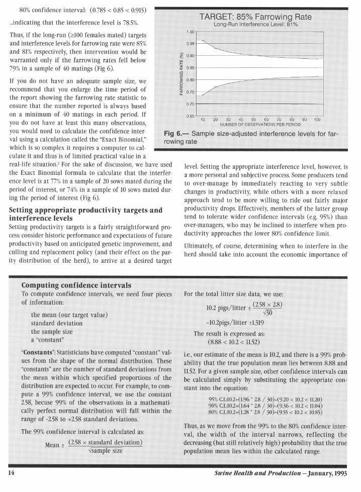
Thus, if the long-run (;:0:100females mated) targetsand interference levels for farrowing rate were 85%and 81%respectively, then intervention would bewarranted only if the farrowing rates fell below79%in a sample of 40 matings (Fig 6).

If you do not have an adequate sample size, werecommend that you enlarge the time period ofthe report showing the farrowing rate statistic toensure that the number reported is always basedon a minimum of 40 matings in each period. Ifyou do not have at least this many observations,you would need to calculate the confidence inter-val using a calculation called the "ExactBinomial,"which is so complex it requires a computer to cal-culate it and thus is of limited practical value in areal-life situation.2For the sake of discussion, we have usedthe Exact Binomial formula to calculate that the interfer-

ence level is at 77%in a sample of 20 sows mated during theperiod of interest, or 74%in a sample of 10sows mated dur-ing the period of interest (Fig 6).

Setting appropriate productivity targets andinterference levelsSetting productivity targets is a fairly straightforward pro-cess:consider historic performance and expectations of futureproductivity based on anticipated genetic improvement, andculling and replacement policy (and their effect on the par-ity distribution of the herd), to arrive at a desired target

level. Setting the appropriate interference level, however, isa more personal and subjective process.Someproducers tendto over-manageby immediately reacting to very subtlechangesin productivity,while others with a more relaxed

\

approach tend to be more willing to ride out fairly majorproductivity drops. Effectively,members of the latter grouptend to tolerate wider confidence intervals (e.g. 95%)thanover-managers,who may be inclined to interfere when pro-ductivity approaches the lower 80%confidence limit.

Ultimately, of course, determining when to interfere in theherd should take into account the economic importance of

14 Swine Health and Production - January,1993

the problem. Even though experienced managers tend toponder economic considerations when adjusting targets andinterference levels, it is important to consider the financialrepercussions of alternative interventions (or doing noth-ing), rather than interfere as a matter of course. In caseswhere the herd is already managed very efficiently, the costand additional risk of interference may outweigh the po-tential expected benefits. Also,because many indicators ofbreeding herd productivity (e.g.,litter size) are affected byseasonal influences and by shifting parity distributions, thesolution to a productivity dip may be to over-breed at cer-tain times of the year, or to maintain the optimal paritydistribution for the herd genetics and production system.As a practitioner, you will need to understand not only howto exploit statistics to help your clients interpret their pro-ductivity data, but you will also need to tailor yourrecommendations to the season, the particular managementpractices in the herd, and the personality of the producer orherd manager.

The simple procedures we have outlined (from plotting datato show distributions, setting feasible production targets,

calculating confidence intervals, to adjusting interferencelevels to compensate for small sample sizes) can improveeffective communication between the herd manager andconsultant. Properly applied, these techniques can help usavoid becoming distracted by spurious production changeswhile improving our power to detect emerging problemsbefore they cause severe economic loss.

References

1. Websters New Twentieth Dictionary. Unabridged 2nd ed.(1979). Prentice Hall Press, New York.

2. Rosner, BR.(1990) Fundamentals of Biostatistics. PWS-KentPublishing Co. Boston.

3. Smith, RS. (1991) Veterinary Clinical Epidemiology: a

problem-oriented approach. Butterworth-Heinemann,Stoneham Massachusetts.

Swine Health and Production - Volume 1,Number 1 15