The Computational Limits of Deep Learning

Neil C. Thompson1∗, Kristjan Greenewald2, Keeheon Lee3, Gabriel F. Manso4

1MIT Computer Science and A.I. Lab,MIT Initiative on the Digital Economy, Cambridge, MA USA

2MIT-IBM Watson AI Lab, Cambridge MA, USA3Underwood International College, Yonsei University, Seoul, Korea

4UnB FGA, University of Brasilia, Brasilia, Brazil

∗To whom correspondence should be addressed; E-mail: neil t@mit.edu.

Deep learning’s recent history has been one of achievement: from triumphing

over humans in the game of Go to world-leading performance in image recog-

nition, voice recognition, translation, and other tasks. But this progress has

come with a voracious appetite for computing power. This article reports on

the computational demands of Deep Learning applications in five prominent

application areas and shows that progress in all five is strongly reliant on in-

creases in computing power. Extrapolating forward this reliance reveals that

progress along current lines is rapidly becoming economically, technically, and

environmentally unsustainable. Thus, continued progress in these applications

will require dramatically more computationally-efficient methods, which will

either have to come from changes to deep learning or from moving to other

machine learning methods.

1

1 Introduction

In this article, we analyze 1,058 research papers found in the arXiv pre-print repository, as

well as other benchmark sources, to understand how deep learning performance depends on

computational power in the domains of image classification, object detection, question answering,

named entity recognition, and machine translation. We show that computational requirements

have escalated rapidly in each of these domains and that these increases in computing power

have been central to performance improvements. If progress continues along current lines,

these computational requirements will rapidly become technically and economically prohibitive.

Thus, our analysis suggests that deep learning progress will be constrained by its computational

requirements and that the machine learning community will be pushed to either dramatically

increase the efficiency of deep learning or to move to more computationally-efficient machine

learning techniques.

To understand why deep learning is so computationally expensive, we analyze its statistical

and computational scaling in theory. We show deep learning is not computationally expensive

by accident, but by design. The same flexibility that makes it excellent at modeling diverse

phenomena and outperforming expert models also makes it dramatically more computationally

expensive. Despite this, we find that the actual computational burden of deep learning models

is scaling more rapidly than (known) lower bounds from theory, suggesting that substantial

improvements might be possible.

It would not be a historical anomaly for deep learning to become computationally constrained.

Even at the creation of the first neural networks by Frank Rosenblatt, performance was limited

by the available computation. In the past decade, these computational constraints have relaxed

due to speed-ups from moving to specialized hardware and a willingness to invest additional

resources to get better performance. But, as we show, the computational needs of deep learning

2

scale so rapidly, that they will quickly become burdensome again.

2 Deep Learning’s Computational Requirements in Theory

The relationship between performance, model complexity, and computational requirements

in deep learning is still not well understood theoretically. Nevertheless, there are important

reasons to believe that deep learning is intrinsically more reliant on computing power than other

techniques, in particular due to the role of overparameterization and how this scales as additional

training data are used to improve performance (including, for example, classification error rate,

root mean squared regression error, etc.).

It has been proven that there are significant benefits to having a neural network contain more

parameters than there are data points available to train it, that is, by overparameterizing it [81].

Classically this would lead to overfitting, but stochastic gradient-based optimization methods

provide a regularizing effect due to early stopping [71, 8]1, moving the neural networks into

an interpolation regime, where the training data is fit almost exactly while still maintaining

reasonable predictions on intermediate points [9, 10]. An example of large-scale overparameteri-

zation is the current state-of-the-art image recognition system, NoisyStudent, which has 480M

parameters for imagenet’s 1.2M data points [94, 77].

The challenge of overparameterization is that the number of deep learning parameters must

grow as the number of data points grows. Since the cost of training a deep learning model

scales with the product of the number of parameters with the number of data points, this

implies that computational requirements grow as at least the square of the number of data

points in the overparameterized setting. This quadratic scaling, however, is an underestimate

of how fast deep learning networks must grow to improve performance, since the amount

of training data must scale much faster than linearly in order to get a linear improvement in

1This is often called implicit regularization, since there is no explicit regularization term in the model.

3

performance. Statistical learning theory tells us that, in general, root mean squared estimation

error can at most drop as 1/√n (where n is the number of data points), suggesting that at least a

quadratic increase in data points would be needed to improve performance, here viewing (possibly

continuous-valued) label prediction as a latent variable estimation problem. This back-of-the

envelope calculation thus implies that the computation required to train an overparameterized

model should grow at least as a fourth-order polynomial with respect to performance, i.e.

Computation = O(Performance4), and may be worse.

The relationship between model parameters, data, and computational requirements in deep

learning can be illustrated by analogy in the setting of linear regression, where the statistical

learning theory is better developed (and, which is equivalent to a 1-layer neural network with

linear activations). Consider the following generative d-dimensional linear model: y(x) =

θTx + z, where z is Gaussian noise. Given n independent (x, y) samples, the least squares

estimate of θ is θLS = (XTX)−1XTY , yielding a predictor y(x0) = θTLSx0 on unseen x0.2 The

root mean squared error of this predictor can be shown3 to scale as O(√

dn

). Suppose that d (the

number of covariates in x) is very large, but we expect that only a few of these covariates (whose

identities we don’t know) are sufficient to achieve good prediction performance. A traditional

approach to estimating θ would be to use a small model, i.e. choosing only some small number

of covariates, s, in x, chosen based on expert guidance about what matters. When such a model

correctly identifies all the relevant covariates (the “oracle” model), a traditional least-squares

estimate of the s covariates is the most efficient unbiased estimate of θ.4 When such a model is

only partially correct and omits some of the relevant covariates from its model, it will quickly

learn the correct parts as n increases but will then have its performance plateau. An alternative

is to attempt to learn the full d-dimensional model by including all covariates as regressors.2X ∈ Rn×d is a matrix concatenating the samples from x, and Y is a n-dimensional vector concatenating the

samples of y.3When both x and x0 are drawn from an isotropic multivariate Gaussian distribution.4Gauss-Markov Theorem.

4

Unfortunately, this flexible model is often too data inefficient to be practical.

Regularization can help. In regression, one of the simplest forms of regularization is the

Lasso [85], which penalizes the number of non-zero coefficients in the model, making it sparser.

Lasso regularization improves the root mean squared error scaling toO(√

s log dn

)where s is the

number of nonzero coefficients in the true model[63]. Hence if s is a constant and d is large, the

data requirements of Lasso is within a logarithmic factor of the oracle model, and exponentially

better than the flexible least squares approach. This improvement allows the regularized model

to be much more flexible (by using larger d), but this comes with the full computational costs

associated with estimating a large number (d) of parameters. Note that while here d is the

dimensionality of the data (which can be quite large, e.g. the number of pixels in an image),

one can also view deep learning as mapping data to a very large number of nonlinear features.

If these features are viewed as d, it is perhaps easier to see why one would want to increase d

dramatically to achieve flexibility (as it would now correspond to the number of neurons in the

network).

To see these trade-offs quantitatively, consider a generative model that has 10 non-zero

parameters out of a possible 1000, and consider 4 models for trying to discover those parameters:

• Oracle model: has exactly the correct 10 parameters in the model

• Expert model: has exactly 9 correct and 1 incorrect parameters in the model

• Flexible model: has all 1000 potential parameters in the model and uses the least-squares

estimate

• Regularized model: like the flexible model, it has all 1000 potential parameters but now

in a regularized (Lasso) model

We measure the performance as − log10(MSE), where MSE is the normalized mean squared

error between the prediction computed using the estimated parameters and the prediction com-

5

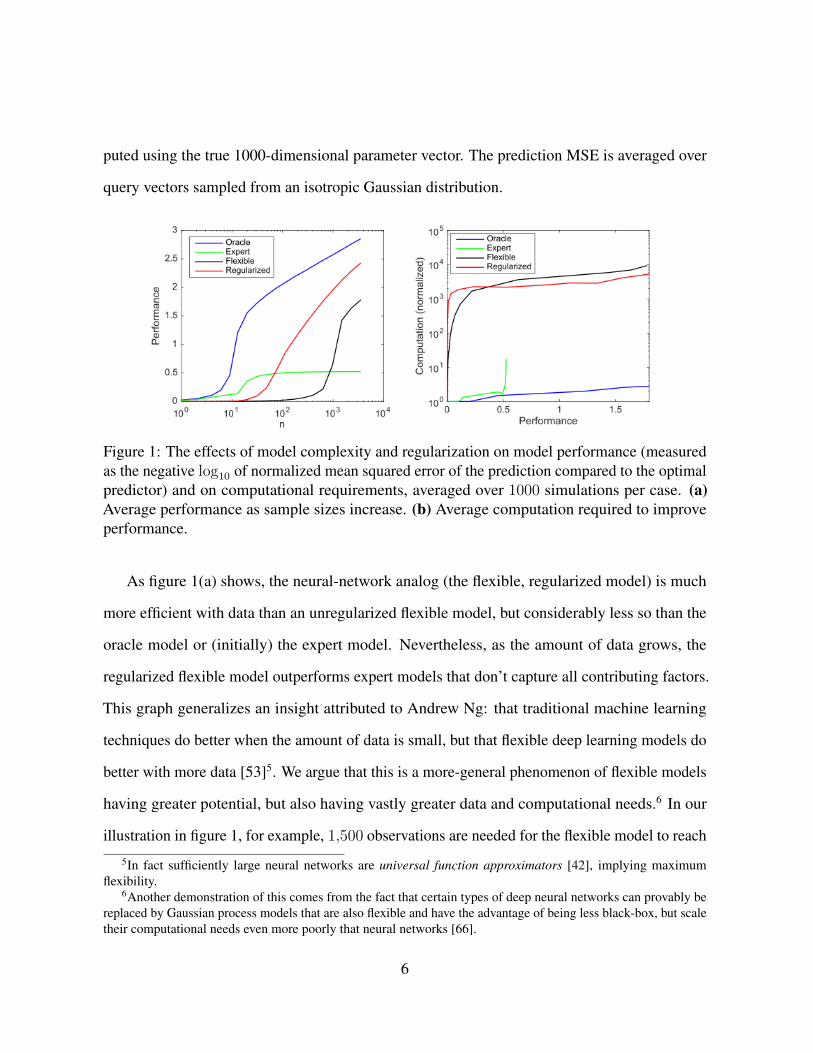
puted using the true 1000-dimensional parameter vector. The prediction MSE is averaged over

query vectors sampled from an isotropic Gaussian distribution.

Figure 1: The effects of model complexity and regularization on model performance (measuredas the negative log10 of normalized mean squared error of the prediction compared to the optimalpredictor) and on computational requirements, averaged over 1000 simulations per case. (a)Average performance as sample sizes increase. (b) Average computation required to improveperformance.

As figure 1(a) shows, the neural-network analog (the flexible, regularized model) is much

more efficient with data than an unregularized flexible model, but considerably less so than the

oracle model or (initially) the expert model. Nevertheless, as the amount of data grows, the

regularized flexible model outperforms expert models that don’t capture all contributing factors.

This graph generalizes an insight attributed to Andrew Ng: that traditional machine learning

techniques do better when the amount of data is small, but that flexible deep learning models do

better with more data [53]5. We argue that this is a more-general phenomenon of flexible models

having greater potential, but also having vastly greater data and computational needs.6 In our

illustration in figure 1, for example, 1,500 observations are needed for the flexible model to reach

5In fact sufficiently large neural networks are universal function approximators [42], implying maximumflexibility.

6Another demonstration of this comes from the fact that certain types of deep neural networks can provably bereplaced by Gaussian process models that are also flexible and have the advantage of being less black-box, but scaletheir computational needs even more poorly that neural networks [66].

6

the same performance as the oracle reaches with 15. Regularization helps with this, dropping the

data need to 175. But, while regularization helps substantially with the pace at which data can be

learned from, it helps much less with the computational costs, as figure 1(b) shows.

Hence, by analogy, we can see that deep learning performs well because it uses overpa-

rameterization to create a highly flexible model and uses (implicit) regularization to make the

sample complexity tractable. At the same time, however, deep learning requires vastly more

computation than more efficient models. Thus, the great flexibility of deep learning inherently

implies a dependence on large amounts of data and computation.

3 Deep Learning’s Computational Requirements in Practice

3.1 Past

Even in their early days, it was clear that computational requirements limited what neural

networks could achieve. In 1960, when Frank Rosenblatt wrote about a 3-layer neural network,

there were hopes that it had “gone a long way toward demonstrating the feasibility of a perceptron

as a pattern-recognizing device.” But, as Rosenblatt already recognized “as the number of

connections in the network increases, however, the burden on a conventional digital computer

soon becomes excessive.” [76] Later that decade, in 1969, Minsky and Papert explained the

limits of 3-layer networks, including the inability to learn the simple XOR function. At the same

time, however, they noted a potential solution: “the experimenters discovered an interesting

way to get around this difficulty by introducing longer chains of intermediate units” (that is, by

building deeper neural networks).[64] Despite this potential workaround, much of the academic

work in this area was abandoned because there simply wasn’t enough computing power available

at the time. As Leon Bottou later wrote “the most obvious application of the perceptron,

computer vision, demands computing capabilities that far exceed what could be achieved with

the technology of the 1960s”.[64]

7

In the decades that followed, improvements in computer hardware provided, by one measure,

a ≈50,000× improvement in performance [39] and neural networks grew their computational

requirements proportionally, as shown in figure 2(a). Since the growth in computing power

per dollar closely mimicked the growth in computing power per chip [84], this meant that the

economic cost of running such models was largely stable over time. Despite this large increase,

deep learning models in 2009 remained “too slow for large-scale applications, forcing researchers

to focus on smaller-scale models or to use fewer training examples.”[73] The turning point seems

to have been when deep learning was ported to GPUs, initially yielding a 5 − 15× speed-up

[73] which by 2012 had grown to more than 35× [1], and which led to the important victory

of Alexnet at the 2012 Imagenet competition [52].7 But image recognition was just the first of

these benchmarks to fall. Shortly thereafter, deep learning systems also won at object detection,

named-entity recognition, machine translation, question answering, and speech recognition.

The introduction of GPU-based (and later ASIC-based) deep learning led to widespread

adoption of these systems. But the amount of computing power used in cutting-edge systems

grew even faster, at approximately 10× per year from 2012 to 2019 [5]. This rate is far faster

than the ≈ 35× total improvement from moving to GPUs, the meager improvements from the

last vestiges of Moore’s Law [84], or the improvements in neural network training efficiency [40].

Instead, much of the increase came from a much-less-economically-attractive source: running

models for more time on more machines. For example, in 2012 AlexNet trained using 2 GPUs

for 5-6 days[52], in 2017 ResNeXt-101 [95] was trained with 8 GPUs for over 10 days, and in

2019 NoisyStudent was trained with ≈ 1,000 TPUs (one TPU v3 Pod) for 6 days[94]. Another

extreme example is the machine translation system, “Evolved Transformer”, which used more

than 2 million GPU hours and cost millions of dollars to run[80, 92]. Scaling deep learning7The ImageNet Large Scale Visual Recognition Challenge (ILSVRC) released a large visual database to evaluate

algorithms for classifying and detecting objects and scenes every year since 2010 [26, 77].8The range of hardware performance values indicates the difference between SPECInt values for the lowest core

counts and SPECIntRate values for the highest core counts.

8

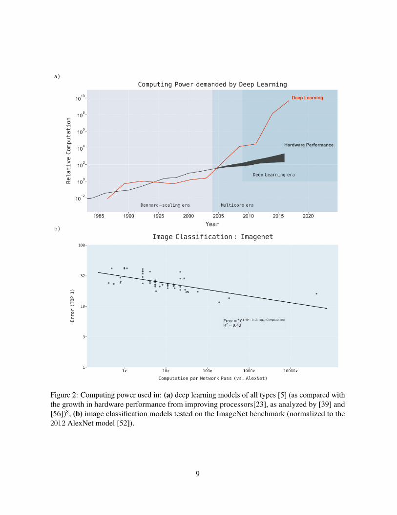
Figure 2: Computing power used in: (a) deep learning models of all types [5] (as compared withthe growth in hardware performance from improving processors[23], as analyzed by [39] and[56])8, (b) image classification models tested on the ImageNet benchmark (normalized to the2012 AlexNet model [52]).

9

computation by scaling up hardware hours or number of chips is problematic in the longer-term

because it implies that costs scale at roughly the same rate as increases in computing power [5],

which (as we show) will quickly make it unsustainable.

3.2 Present

To examine deep learning’s dependence on computation, we examine 1,058 research papers,

covering the domains of image classification (ImageNet benchmark), object detection (MS

COCO), question answering (SQuAD 1.1), named-entity recognition (COLLN 2003), and

machine translation (WMT 2014 En-to-Fr). We also investigated models for CIFAR-10, CIFAR-

100, and ASR SWB Hub500 speech recognition, but too few of the papers in these areas reported

computational details to analyze those trends.

We source deep learning papers from the arXiv repository as well as other benchmark sources

(see Section 6 in the supplement for more information on the data gathering process). In many

cases, papers did not report any details of their computational requirements. In other cases

only limited computational information was provided. As such, we do two separate analyses

of computational requirements, reflecting the two types of information that were available: (1)

Computation per network pass (the number of floating point operations required for a single pass

in the network, also measurable using multiply-adds or the number of parameters in the model),

and (2) Hardware burden (the computational capability of the hardware used to train the model,

calculated as #processors× ComputationRate× time).

We demonstrate our analysis approach first in the area with the most data and longest history:

image classification. As opposed to the previous section where we considered mean squared

error, here the relevant performance metric is classification error rate. While not always directly

equivalent, we argue that applying similar forms of analysis to these different performance

10

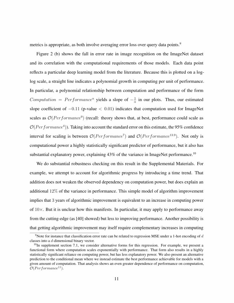
metrics is appropriate, as both involve averaging error loss over query data points.9

Figure 2 (b) shows the fall in error rate in image recognition on the ImageNet dataset

and its correlation with the computational requirements of those models. Each data point

reflects a particular deep learning model from the literature. Because this is plotted on a log-

log scale, a straight line indicates a polynomial growth in computing per unit of performance.

In particular, a polynomial relationship between computation and performance of the form

Computation = Performanceα yields a slope of − 1α

in our plots. Thus, our estimated

slope coefficient of −0.11 (p-value < 0.01) indicates that computation used for ImageNet

scales as O(Performance9) (recall: theory shows that, at best, performance could scale as

O(Performance4)). Taking into account the standard error on this estimate, the 95% confidence

interval for scaling is between O(Performance7) and O(Performance13.9). Not only is

computational power a highly statistically significant predictor of performance, but it also has

substantial explanatory power, explaining 43% of the variance in ImageNet performance.10

We do substantial robustness checking on this result in the Supplemental Materials. For

example, we attempt to account for algorithmic progress by introducing a time trend. That

addition does not weaken the observed dependency on computation power, but does explain an

additional 12% of the variance in performance. This simple model of algorithm improvement

implies that 3 years of algorithmic improvement is equivalent to an increase in computing power

of 10×. But it is unclear how this manifests. In particular, it may apply to performance away

from the cutting-edge (as [40] showed) but less to improving performance. Another possibility is

that getting algorithmic improvement may itself require complementary increases in computing9Note for instance that classification error rate can be related to regression MSE under a 1-hot encoding of d

classes into a d-dimensional binary vector.10In supplement section 7.1, we consider alternative forms for this regression. For example, we present a

functional form where computation scales exponentially with performance. That form also results in a highlystatistically significant reliance on computing power, but has less explanatory power. We also present an alternativeprediction to the conditional mean where we instead estimate the best performance achievable for models with agiven amount of computation. That analysis shows an even greater dependence of performance on computation,O(Performance11).

11

power.

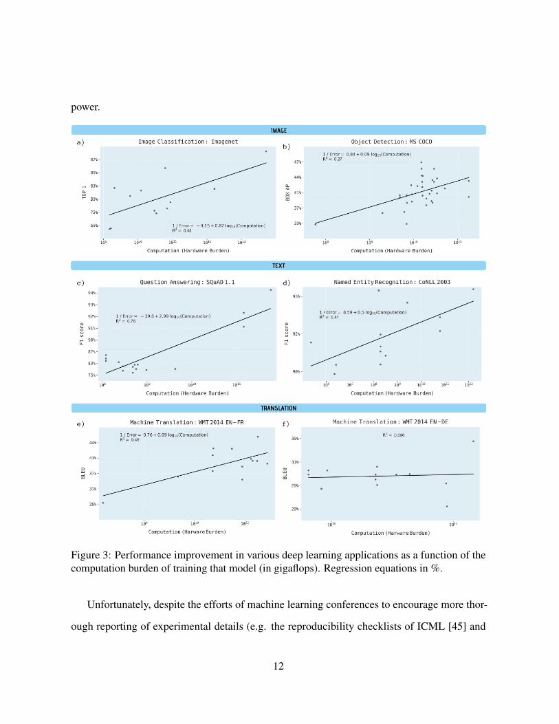
Figure 3: Performance improvement in various deep learning applications as a function of thecomputation burden of training that model (in gigaflops). Regression equations in %.

Unfortunately, despite the efforts of machine learning conferences to encourage more thor-

ough reporting of experimental details (e.g. the reproducibility checklists of ICML [45] and

12

NeurIPS), few papers in the other benchmark areas provide sufficient information to analyze

the computation needed per network pass. More widely reported, however, is the computational

hardware burden of running models. This also estimates the computation needed, but is less

precise since it depends on hardware implementation efficiency.

Figure 3 shows progress in the areas of image classification, object detection, question

answering, named entity recognition, and machine translation. We find highly-statistically

significant slopes and strong explanatory power (R2 between 29% and 68%) for all benchmarks

except machine translation, English to German, where we have very little variation in the

computing power used. Interpreting the coefficients for the five remaining benchmarks shows a

slightly higher polynomial dependence for imagenet when calculated using this method (≈ 14),

and a dependence of 7.7 for question answering. Object detection, named-entity recognition and

machine translation show large increases in hardware burden with relatively small improvements

in outcomes, implying dependencies of around 50. We test other functional forms in the

supplementary materials and, again, find that overall the polynomial models best explain this

data, but that models implying an exponential increase in computing power as the right functional

form are also plausible.

Collectively, our results make it clear that, across many areas of deep learning, progress in

training models has depended on large increases in the amount of computing power being used.

A dependence on computing power for improved performance is not unique to deep learning,

but has also been seen in other areas such as weather prediction and oil exploration [83]. But

in those areas, as might be a concern for deep learning, there has been enormous growth in the

cost of systems, with many cutting-edge models now being run on some of the largest computer

systems in the world.

13

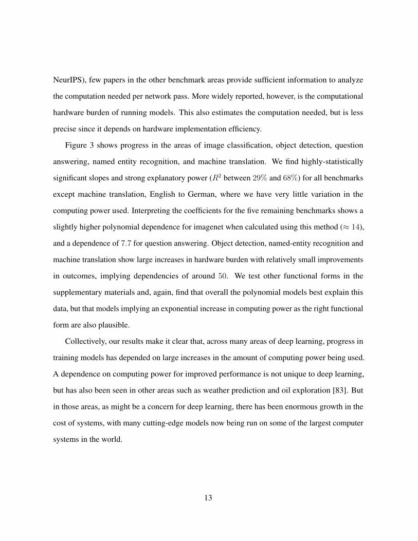
3.3 Future

In this section, we extrapolate the estimates from each domain to understand the projected

computational power needed to hit various benchmarks. To make these targets tangible, we

present them not only in terms of the computational power required, but also in terms of

the economic and environmental cost of training such models on current hardware (using the

conversions from [82]). Because the polynomial and exponential functional forms have roughly

equivalent statistical fits — but quite different extrapolations — we report both in figure 4.

Figure 4: Implications of achieving performance benchmarks on the computation (in Gigaflops),carbon emissions (lbs), and economic costs ($USD) from deep learning based on projections frompolynomial and exponential models. The carbon emissions and economic costs of computingpower usage are calculated using the conversions from [82]

We do not anticipate that the computational requirements implied by the targets in

figure 4 will be hit. The hardware, environmental, and monetary costs would be prohibitive.

And enormous effort is going into improving scaling performance, as we discuss in the next

section. But, these projections do provide a scale for the efficiency improvements that would be

14

needed to hit these performance targets. For example, even in the more-optimistic model, it is

estimated to take an additional 105× more computing to get to an error rate of 5% for ImageNet.

Hitting this in an economical way will require more efficient hardware, more efficient algorithms,

or other improvements such that the net impact is this large a gain.

The rapid escalation in computing needs in figure 4 also makes a stronger statement: along

current trends, it will not be possible for deep learning to hit these benchmarks. Instead,

fundamental rearchitecting is needed to lower the computational intensity so that the scaling of

these problems becomes less onerous. And there is promise that this could be achieved. Theory

tells us that the lower bound for the computational intensity of regularized flexible models is

O(Performance4), which is much better than current deep learning scaling. Encouragingly,

there is historical precedent for algorithms improving rapidly [79].

4 Lessening the Computational Burden

The economic and environmental burden of hitting the performance benchmarks in Section

3.3 suggest that Deep Learning is facing an important challenge: either find a way to increase

performance without increasing computing power, or have performance stagnate as computational

requirements become a constraint. In this section, we briefly survey approaches that are being

used to address this challenge.

Increasing computing power: Hardware accelerators. For much of the 2010s, moving to

more-efficient hardware platforms (and more of them) was a key source of increased computing

power [84]. For deep learning, these included mostly GPU and TPU implementations, although

it has increasingly also included FPGA and other ASICs. Fundamentally, all of these approaches

sacrifice generality of the computing platform for the efficiency of increased specialization. But

such specialization faces diminishing returns [56], and so other different hardware frameworks

are being explored. These include analog hardware with in-memory computation [3, 47], neu-

15

romorphic computing [25], optical computing [58], and quantum computing based approaches

[90], as well as hybrid approaches [72]. Thus far, however, such attempts have yet to disrupt the

GPU/TPU and FPGA/ASIC architectures. Of these, quantum computing is the approach with

perhaps the most long-term upside, since it offers a potential for sustained exponential increases

in computing power [32, 22].

Reducing computational complexity: Network Compression and Acceleration. This

body of work primarily focuses on taking a trained neural network and sparsifying or otherwise

compressing the connections in the network, so that it requires less computation to use it in

prediction tasks [18]. This is typically done by using optimization or heuristics such as “pruning”

away weights [27], quantizing the network [44], or using low-rank compression [91], yielding a

network that retains the performance of the original network but requires fewer floating point

operations to evaluate. Thus far these approaches have produced computational improvements

that, while impressive, are not sufficiently large in comparison to the overall orders-of-magnitude

increases of computation in the field (e.g. the recent work [17] reduces computation by a

factor of 2, and [92] reduces it by a factor of 8 on a specific NLP architecture, both without

reducing performance significantly).11 Furthermore, many of these works focus on improving

the computational cost of evaluating the deployed network, which is useful, but does not mitigate

the training cost, which can also be prohibitive.

Finding high-performing small deep learning architectures: Neural Architecture Search

and Meta Learning. Recently, it has become popular to use optimization to find network archi-

tectures that are computationally efficient to train while retaining good performance on some

class of learning problems, e.g. [70], [13] and [31], as well as exploiting the fact that many

datasets are similar and therefore information from previously trained models can be used (meta

learning [70] and transfer learning [60]). While often quite successful, the current downside is11Some works, e.g. [36] focus more on the reduction in the memory footprint of the model. [36] achieved 50x

compression.

16

that the overhead of doing meta learning or neural architecture search is itself computationally

intense (since it requires training many models on a wide variety of datasets) [70], although the

cost has been decreasing towards the cost of traditional training [14, 13].

An important limitation to meta learning is the scope of the data that the original model

was trained on. For example, for ImageNet, [7] showed that image recognition performance

depends heavily on image biases (e.g. an object is often photographed at a particular angle with

a particular pose), and that without these biases transfer learning performance drops 45%. Even

with novel data sets purposely built to mimic their training data, [75] finds that performance

drops 11− 14%. Hence, while there seems to be a number of promising research directions for

making deep learning computation grow at a more attractive rate, they have yet to achieve the

orders-of-magnitude improvements needed to allow deep learning progress to continue scaling.

Another possible approach to evade the computational limits of deep learning would be

to move to other, perhaps as yet undiscovered or underappreciated types of machine learning.

As figure 1(b) showed, “expert” models can be much more computationally-efficient, but their

performance plateaus if those experts cannot see all the contributing factors that a flexible model

might explore. One example where such techniques are already outperforming deep learning

models are those where engineering and physics knowledge can be more-directly applied: the

recognition of known objects (e.g. vehicles) [38, 86]. The recent development of symbolic

approaches to machine learning take this a step further, using symbolic methods to efficiently

learn and apply “expert knowledge” in some sense, e.g. [87] which learns physics laws from

data, or approaches [62, 6, 96] which apply neuro-symbolic reasoning to scene understanding,

reinforcement learning, and natural language processing tasks, building a high-level symbolic

representation of the system in order to be able to understand and explore it more effectively

with less data.

17

5 Conclusion

The explosion in computing power used for deep learning models has ended the “AI winter”

and set new benchmarks for computer performance on a wide range of tasks. However, deep

learning’s prodigious appetite for computing power imposes a limit on how far it can improve

performance in its current form, particularly in an era when improvements in hardware perfor-

mance are slowing. This article shows that the computational limits of deep learning will soon

be constraining for a range of applications, making the achievement of important benchmark

milestones impossible if current trajectories hold. Finally, we have discussed the likely impact

of these computational limits: forcing Deep Learning towards less computationally-intensive

methods of improvement, and pushing machine learning towards techniques that are more

computationally-efficient than deep learning.

Acknowledgement

The authors would like to acknowledge funding from the MIT Initiative on the Digital Economy

and the Korean Government. This research was partially supported by Basic Science Research

Program through the National Research Foundation of Korea(NRF) funded by the Ministry of

Science, ICT & Future Planning(2017R1C1B1010094).

References

[1] Tesla P100 Performance Guide - HPC and Deep Learning Applications. NVIDIA Corpora-

tion, 2017.

[2] Timo Ahonen, Abdenour Hadid, and Matti Pietikainen. Face description with local binary

patterns: Application to face recognition. IEEE transactions on pattern analysis and

machine intelligence, 28(12):2037–2041, 2006.

18

[3] Stefano Ambrogio, Pritish Narayanan, Hsinyu Tsai, Robert M Shelby, Irem Boybat,

Carmelo di Nolfo, Severin Sidler, Massimo Giordano, Martina Bodini, Nathan CP Farinha,

et al. Equivalent-accuracy accelerated neural-network training using analogue memory.

Nature, 558(7708):60–67, 2018.

[4] Dario Amodei, Sundaram Ananthanarayanan, Rishita Anubhai, Jingliang Bai, Eric Bat-

tenberg, Carl Case, Jared Casper, Bryan Catanzaro, Qiang Cheng, Guoliang Chen, et al.

Deep speech 2: End-to-end speech recognition in english and mandarin. In International

conference on machine learning, pages 173–182, 2016.

[5] Dario Amodei and Danny Hernandez. Ai and compute. 2018.

[6] Masataro Asai and Christian Muise. Learning neural-symbolic descriptive planning models

via cube-space priors: The voyage home (to strips). arXiv preprint arXiv:2004.12850,

2020.

[7] Andrei Barbu, David Mayo, Julian Alverio, William Luo, Christopher Wang, Dan Gutfre-

und, Josh Tenenbaum, and Boris Katz. Objectnet: A large-scale bias-controlled dataset for

pushing the limits of object recognition models. In H. Wallach, H. Larochelle, A. Beygelz-

imer, F. Alche-Buc, E. Fox, and R. Garnett, editors, Advances in Neural Information

Processing Systems 32, pages 9453–9463. Curran Associates, Inc., 2019.

[8] Mikhail Belkin, Daniel Hsu, Siyuan Ma, and Soumik Mandal. Reconciling modern

machine-learning practice and the classical bias–variance trade-off. Proceedings of the

National Academy of Sciences, 116(32):15849–15854, 2019.

[9] Mikhail Belkin, Daniel J Hsu, and Partha Mitra. Overfitting or perfect fitting? risk bounds

for classification and regression rules that interpolate. In Advances in Neural Information

Processing Systems, pages 2300–2311, 2018.

19

[10] Mikhail Belkin, Alexander Rakhlin, and Alexandre B Tsybakov. Does data interpolation

contradict statistical optimality? In The 22nd International Conference on Artificial

Intelligence and Statistics, pages 1611–1619, 2019.

[11] Parminder Bhatia, Busra Celikkaya, Mohammed Khalilia, and Selvan Senthivel. Compre-

hend medical: a named entity recognition and relationship extraction web service. arXiv

preprint arXiv:1910.07419, 2019.

[12] Ondrej Bojar, Christian Buck, Christian Federmann, Barry Haddow, Philipp Koehn, Jo-

hannes Leveling, Christof Monz, Pavel Pecina, Matt Post, Herve Saint-Amand, et al.

Findings of the 2014 workshop on statistical machine translation. In Proceedings of the

ninth workshop on statistical machine translation, pages 12–58, 2014.

[13] Han Cai, Chuang Gan, Tianzhe Wang, Zhekai Zhang, and Song Han. Once for all: Train

one network and specialize it for efficient deployment. In International Conference on

Learning Representations, 2020.

[14] Han Cai, Ligeng Zhu, and Song Han. ProxylessNAS: Direct neural architecture search on

target task and hardware. In International Conference on Learning Representations, 2019.

[15] Mauro Cettolo, Jan Niehues, Sebastian Stuker, Luisa Bentivogli, and Marcello Federico. Re-

port on the 11th iwslt evaluation campaign, iwslt 2014. In Proceedings of the International

Workshop on Spoken Language Translation, Hanoi, Vietnam, volume 57, 2014.

[16] William Chan, Navdeep Jaitly, Quoc Le, and Oriol Vinyals. Listen, attend and spell: A

neural network for large vocabulary conversational speech recognition. In 2016 IEEE

International Conference on Acoustics, Speech and Signal Processing (ICASSP), pages

4960–4964. IEEE, 2016.

20

[17] Chun-Fu Chen, Quanfu Fan, Neil Mallinar, Tom Sercu, and Rogerio Feris. Big-little net:

An efficient multi-scale feature representation for visual and speech recognition. arXiv

preprint arXiv:1807.03848, 2018.

[18] Yu Cheng, Duo Wang, Pan Zhou, and Tao Zhang. A survey of model compression and

acceleration for deep neural networks. arXiv preprint arXiv:1710.09282, 2017.

[19] Adam Coates, Andrew Ng, and Honglak Lee. An analysis of single-layer networks in

unsupervised feature learning. In Proceedings of the fourteenth international conference

on artificial intelligence and statistics, pages 215–223, 2011.

[20] Gregory Cohen, Saeed Afshar, Jonathan Tapson, and Andre Van Schaik. Emnist: Extending

mnist to handwritten letters. In 2017 International Joint Conference on Neural Networks

(IJCNN), pages 2921–2926. IEEE, 2017.

[21] Linguistic Data Consortium. 2000 hub5 english evaluation speech ldc2002s09. Web

Download]. Linguistic Data Consortium, Philadelphia, PA, USA, 2002.

[22] Andrew W Cross, Lev S Bishop, Sarah Sheldon, Paul D Nation, and Jay M Gambetta.

Validating quantum computers using randomized model circuits. Physical Review A,

100(3):032328, 2019.

[23] Andrew Danowitz, Kyle Kelley, James Mao, John P. Stevenson, and Mark Horowitz. CPU

DB: Recording microprocessor history. Queue, 10(4):10:10–10:27, 2012.

[24] Luke N Darlow, Elliot J Crowley, Antreas Antoniou, and Amos J Storkey. Cinic-10 is not

imagenet or cifar-10. arXiv preprint arXiv:1810.03505, 2018.

[25] Mike Davies. Progress in neuromorphic computing: Drawing inspiration from nature for

21

gains in ai and computing. In 2019 International Symposium on VLSI Technology, Systems

and Application (VLSI-TSA), pages 1–1. IEEE, 2019.

[26] J. Deng, W. Dong, R. Socher, L.-J. Li, K. Li, and L. Fei-Fei. ImageNet: A Large-Scale

Hierarchical Image Database. In Conference on Computer Vision and Pattern Recognition,

2009.

[27] Xuanyi Dong, Junshi Huang, Yi Yang, and Shuicheng Yan. More is less: A more compli-

cated network with less inference complexity. In Proceedings of the IEEE Conference on

Computer Vision and Pattern Recognition, pages 5840–5848, 2017.

[28] SM Ali Eslami, Nicolas Heess, Theophane Weber, Yuval Tassa, David Szepesvari, Geof-

frey E Hinton, et al. Attend, infer, repeat: Fast scene understanding with generative models.

In Advances in Neural Information Processing Systems, pages 3225–3233, 2016.

[29] Mark Everingham and John Winn. The pascal visual object classes challenge 2012

(voc2012) development kit. Pattern Analysis, Statistical Modelling and Computational

Learning, Tech. Rep, 2011.

[30] Li Fei-Fei, R Fergus, and P Perona. Caltech 101 dataset. URL: http://www. vision. caltech.

edu/Image Datasets/Caltech101/Caltech101. html, 2004.

[31] Chelsea Finn, Pieter Abbeel, and Sergey Levine. Model-agnostic meta-learning for fast

adaptation of deep networks. In Proceedings of the 34th International Conference on

Machine Learning-Volume 70, pages 1126–1135. JMLR. org, 2017.

[32] J Gambetta and S Sheldon. Cramming more power into a quantum device. IBM Research

Blog, 2019.

22

[33] Alex Graves, Santiago Fernandez, Faustino Gomez, and Jurgen Schmidhuber. Connec-

tionist temporal classification: labelling unsegmented sequence data with recurrent neural

networks. In Proceedings of the 23rd international conference on Machine learning, pages

369–376, 2006.

[34] Alex Graves and Navdeep Jaitly. Towards end-to-end speech recognition with recurrent

neural networks. In International conference on machine learning, pages 1764–1772, 2014.

[35] Gregory Griffin, Alex Holub, and Pietro Perona. Caltech-256 object category dataset. 2007.

[36] Song Han, Huizi Mao, and William J Dally. Deep compression: Compressing deep

neural networks with pruning, trained quantization and huffman coding. arXiv preprint

arXiv:1510.00149, 2015.

[37] Kaiming He, Xiangyu Zhang, Shaoqing Ren, and Jian Sun. Deep residual learning for

image recognition. In Proceedings of the IEEE conference on computer vision and pattern

recognition, pages 770–778, 2016.

[38] Tong He and Stefano Soatto. Mono3d+: Monocular 3d vehicle detection with two-scale 3d

hypotheses and task priors. Proceedings of the AAAI Conference on Artificial Intelligence,

33:8409–8416, July 2019.

[39] John L. Hennessy and David A. Patterson. Computer Architecture: A Quantitative Approach.

Morgan Kaufmann, San Francisco, CA, sixth edition, 2019.

[40] Danny Hernandez and Tom Brown. Ai and efficiency. 2020.

[41] Sepp Hochreiter and Jurgen Schmidhuber. Long short-term memory. Neural computation,

9(8):1735–1780, 1997.

23

[42] Kurt Hornik, Maxwell Stinchcombe, Halbert White, et al. Multilayer feedforward networks

are universal approximators. Neural networks, 2(5):359–366, 1989.

[43] Yanping Huang, Youlong Cheng, Ankur Bapna, Orhan Firat, Dehao Chen, Mia Chen,

HyoukJoong Lee, Jiquan Ngiam, Quoc V Le, and Yonghui Wu. Gpipe: Efficient training

of giant neural networks using pipeline parallelism. In Advances in Neural Information

Processing Systems, pages 103–112, 2019.

[44] Itay Hubara, Matthieu Courbariaux, Daniel Soudry, Ran El-Yaniv, and Yoshua Bengio.

Binarized neural networks. In Advances in neural information processing systems, pages

4107–4115, 2016.

[45] ICML. Icml author guidelines. 2020.

[46] Frederick Jelinek. Continuous speech recognition by statistical methods. Proceedings of

the IEEE, 64(4):532–556, 1976.

[47] W Kim, RL Bruce, T Masuda, GW Fraczak, N Gong, P Adusumilli, S Ambrogio, H Tsai,

J Bruley, J-P Han, et al. Confined pcm-based analog synaptic devices offering low resistance-

drift and 1000 programmable states for deep learning. In Symposium on VLSI Technology,

pages T66–T67. IEEE, 2019.

[48] Jonathan Krause, Jia Deng, Michael Stark, and Li Fei-Fei. Collecting a large-scale dataset

of fine-grained cars. 2013.

[49] Alex Krizhevsky and Geoff Hinton. Convolutional deep belief networks on cifar-10.

Unpublished manuscript, 40(7):1–9, 2010.

[50] Alex Krizhevsky and Geoffrey Hinton. Learning multiple layers of features from tiny

images. Citeseer, 2009.

24

[51] Alex Krizhevsky, Vinod Nair, and Geoffrey Hinton. The cifar-10 dataset. online: http://www.

cs. toronto. edu/kriz/cifar. html, 55, 2014.

[52] Alex Krizhevsky, Ilya Sutskever, and Geoffrey E Hinton. Imagenet classification with deep

convolutional neural networks. In Advances in Neural Information Processing Systems,

pages 1097–1105, 2012.

[53] Karin Kruup. Clearing the buzzwords in machine learning, May 2018.

[54] Alex Lamb, Asanobu Kitamoto, David Ha, Kazuaki Yamamoto, Mikel Bober-Irizar, and

Tarin Clanuwat. Deep learning for classical japanese literature. 2018.

[55] Yann LeCun, Corinna Cortes, and Christopher JC Burges. The mnist database of handwrit-

ten digits, 1998. URL http://yann. lecun. com/exdb/mnist, 10:34, 1998.

[56] Charles E. Leiserson, Neil C. Thompson, Joel Emer, Bradley C. Kuszmaul, Butler W.

Lampson, Daniel Sanchez, and Tao B. Schardl. Theres plenty of room at the top: What

will drive growth in computer performance after moores law ends? Science, 2020.

[57] Tsung-Yi Lin, Michael Maire, Serge Belongie, James Hays, Pietro Perona, Deva Ramanan,

Piotr Dollar, and C Lawrence Zitnick. Microsoft coco: Common objects in context. In

European conference on computer vision, pages 740–755. Springer, 2014.

[58] Xing Lin, Yair Rivenson, Nezih T Yardimci, Muhammed Veli, Yi Luo, Mona Jarrahi,

and Aydogan Ozcan. All-optical machine learning using diffractive deep neural networks.

Science, 361(6406):1004–1008, 2018.

[59] Yuanqing Lin, Fengjun Lv, Shenghuo Zhu, Ming Yang, Timothee Cour, Kai Yu, Liangliang

Cao, and Thomas Huang. Large-scale image classification: Fast feature extraction and svm

training. In CVPR 2011, pages 1689–1696. IEEE, 2011.

25

[60] Mingsheng Long, Han Zhu, Jianmin Wang, and Michael I Jordan. Deep transfer learning

with joint adaptation networks. In Proceedings of the 34th International Conference on

Machine Learning-Volume 70, pages 2208–2217. JMLR. org, 2017.

[61] David G Lowe. Distinctive image features from scale-invariant keypoints. International

journal of computer vision, 60(2):91–110, 2004.

[62] Jiayuan Mao, Chuang Gan, Pushmeet Kohli, Joshua B Tenenbaum, and Jiajun Wu. The

neuro-symbolic concept learner: Interpreting scenes, words, and sentences from natural

supervision. arXiv preprint arXiv:1904.12584, 2019.

[63] Nicolai Meinshausen and Bin Yu. Lasso-type recovery of sparse representations for high-

dimensional data. The Annals of Statistics, 37(1):246–270, 2009.

[64] Marvin Minsky and Seymour Papert. Perceptrons: An Introduction to Computational

Geometry. MIT Press, Cambridge, MA, USA, 1969.

[65] Yuval Netzer, Tao Wang, Adam Coates, Alessandro Bissacco, Bo Wu, and A Ng. The street

view house numbers (svhn) dataset, 2019.

[66] Roman Novak, Lechao Xiao, Jaehoon Lee, Yasaman Bahri, Greg Yang, Jiri Hron, Daniel A.

Abolafia, Jeffrey Pennington, and Jascha Sohl-Dickstein. Bayesian deep convolutional

networks with many channels are gaussian processes, 2018.

[67] Kishore Papineni, Salim Roukos, Todd Ward, and Wei-Jing Zhu. Bleu: a method for

automatic evaluation of machine translation. In Proceedings of the 40th annual meeting on

association for computational linguistics, pages 311–318. Association for Computational

Linguistics, 2002.

26

[68] Florent Perronnin and Christopher Dance. Fisher kernels on visual vocabularies for image

categorization. In 2007 IEEE conference on computer vision and pattern recognition, pages

1–8. IEEE, 2007.

[69] Florent Perronnin, Jorge Sanchez, and Thomas Mensink. Improving the fisher kernel

for large-scale image classification. In European conference on computer vision, pages

143–156. Springer, 2010.

[70] Hieu Pham, Melody Guan, Barret Zoph, Quoc Le, and Jeff Dean. Efficient neural archi-

tecture search via parameters sharing. In International Conference on Machine Learning,

pages 4095–4104, 2018.

[71] Loucas Pillaud-Vivien, Alessandro Rudi, and Francis Bach. Statistical optimality of

stochastic gradient descent on hard learning problems through multiple passes. In Advances

in Neural Information Processing Systems, pages 8125–8135, 2018.

[72] Thomas E Potok, Catherine Schuman, Steven Young, Robert Patton, Federico Spedalieri,

Jeremy Liu, Ke-Thia Yao, Garrett Rose, and Gangotree Chakma. A study of complex deep

learning networks on high-performance, neuromorphic, and quantum computers. ACM

Journal on Emerging Technologies in Computing Systems (JETC), 14(2):1–21, 2018.

[73] Rajat Raina, Anand Madhavan, and Andrew Ng. Large-scale deep unsupervised learning

using graphics processors. Proceedings of the 26th International Conference on Machine

Learning, 2009.

[74] Pranav Rajpurkar, Jian Zhang, Konstantin Lopyrev, and Percy Liang. Squad: 100,000+

questions for machine comprehension of text. In Proceedings of the 2016 Conference on

Empirical Methods in Natural Language Processing, pages 2383–2392, 2016.

27

[75] Benjamin Recht, Rebecca Roelofs, Ludwig Schmidt, and Vaishaal Shankar. Do imagenet

classifiers generalize to imagenet?, 2019.

[76] Frank Rosenblatt. Perceptron simulation experiments. Proceedings of the IRE, 48(3):301–

309, March 1960.

[77] Olga Russakovsky, Jia Deng, Hao Su, Jonathan Krause, Sanjeev Satheesh, Sean Ma,

Zhiheng Huang, Andrej Karpathy, Aditya Khosla, Michael Bernstein, Alexander Berg, and

Li Fei-Fei. Imagenet large scale visual recognition challenge. International Journal of

Computer Vision, 115(3):211–252, 2015.

[78] Erik F Sang and Fien De Meulder. Introduction to the conll-2003 shared task: Language-

independent named entity recognition. arXiv preprint cs/0306050, 2003.

[79] Yash Sherry and Neil Thompson. How fast do algorithms improve? Mimeo, 2020.

[80] Le Quoc So, David and Chen Liang. The evolved transformer. ICML, 2019.

[81] Mahdi Soltanolkotabi, Adel Javanmard, and Jason D Lee. Theoretical insights into the

optimization landscape of over-parameterized shallow neural networks. IEEE Transactions

on Information Theory, 65(2):742–769, 2019.

[82] Emma Strubell, Ananya Ganesh, and Andrew McCallum. Energy and policy considerations

for deep learning in nlp. arXiv preprint arXiv:1906.02243, 2019.

[83] Neil Thompson, Shuning Ge, and Gabriel Filipe. The importance of (exponentially more)

computing power. Mimeo, 2020.

[84] Neil Thompson and Svenja Spanuth. The decline of computers as a general purpose

technology: Why deep learning and the end of moores law are fragmenting computing.

Available at SSRN 3287769, 2018.

28

[85] Robert Tibshirani. Regression shrinkage and selection via the lasso. Journal of the Royal

Statistical Society: Series B (Methodological), 58(1):267–288, 1996.

[86] Vasileios Tzoumas, Pasquale Antonante, and Luca Carlone. Outlier-robust spatial percep-

tion: Hardness, general-purpose algorithms, and guarantees. 2019.

[87] Silviu-Marian Udrescu and Max Tegmark. Ai feynman: A physics-inspired method for

symbolic regression. Science Advances, 6(16):eaay2631, 2020.

[88] Grant Van Horn, Oisin Mac Aodha, Yang Song, Yin Cui, Chen Sun, Alex Shepard, Hartwig

Adam, Pietro Perona, and Serge Belongie. The inaturalist species classification and

detection dataset. In Proceedings of the IEEE conference on computer vision and pattern

recognition, pages 8769–8778, 2018.

[89] Jinjun Wang, Jianchao Yang, Kai Yu, Fengjun Lv, Thomas Huang, and Yihong Gong.

Locality-constrained linear coding for image classification. In 2010 IEEE computer society

conference on computer vision and pattern recognition, pages 3360–3367. IEEE, 2010.

[90] J Welser, JW Pitera, and C Goldberg. Future computing hardware for ai. In 2018 IEEE

International Electron Devices Meeting (IEDM), pages 1–3. IEEE, 2018.

[91] Wei Wen, Cong Xu, Chunpeng Wu, Yandan Wang, Yiran Chen, and Hai Li. Coordinating

filters for faster deep neural networks. In Proceedings of the IEEE International Conference

on Computer Vision, pages 658–666, 2017.

[92] Zhanghao Wu, Zhijian Liu, Ji Lin, Yujun Lin, and Song Han. Lite transformer with long-

short range attention. In International Conference on Learning Representations (ICLR),

2020.

29

[93] Han Xiao, Kashif Rasul, and Roland Vollgraf. Fashion-mnist: a novel image dataset for

benchmarking machine learning algorithms. arXiv preprint arXiv:1708.07747, 2017.

[94] Qizhe Xie, Eduard Hovy, Minh-Thang Luong, and Quoc V Le. Self-training with noisy

student improves imagenet classification. arXiv preprint arXiv:1911.04252, 2019.

[95] Saining Xie, Ross Girshick, Piotr Dollar, Zhuowen Tu, and Kaiming He. Aggregated

residual transformations for deep neural networks. In Proceedings of the IEEE conference

on computer vision and pattern recognition, pages 1492–1500, 2017.

[96] Kexin Yi, Jiajun Wu, Chuang Gan, Antonio Torralba, Pushmeet Kohli, and Josh Tenenbaum.

Neural-symbolic vqa: Disentangling reasoning from vision and language understanding. In

Advances in Neural Information Processing Systems, pages 1031–1042, 2018.

[97] Xi Zhou, Kai Yu, Tong Zhang, and Thomas S Huang. Image classification using super-

vector coding of local image descriptors. In European conference on computer vision,

pages 141–154. Springer, 2010.

30

Supplemental Materials

6 Methodology

6.1 Data collection

We collect data on the performance and computational requirements of various deep learning

models from arXiv (arXiv.org), which is an open-access archive where scholars upload

preprints of their scientific papers (once they are approved by moderators). Preprints are catego-

rized into the following fields: mathematics, physics, astrophysics, computer science, quantitative

biology, quantitative finance, statistics, electrical engineering and systems science, and eco-

nomics. Moderators review submissions and can (re)categorize them or reject them (but this is

not a full peer review), as discussed at https://arxiv.org/corr/subjectclasses.

Preprints are accessible and freely distributed worldwide.

To collect preprints of interest from arXiv, we use the search terms of specific tasks and

benchmarks (as discussed below). These allow us to gather pdf pre-prints from arXiv.org.

From each paper, we attempt to gather the following pieces of information:

• Application area (e.g. image recognition)

• Benchmark (name, version, # of items in the training set)

• Paper details (authors, title, year made public, model name)

• Model performance

• Computational requirements (# floating-point operations, # multiply-adds)

• Hardware usage (hardware type, hardware performance (GFLOPs), # processors, running

time)

1

• Network characteristics (# parameters, # of training epochs)

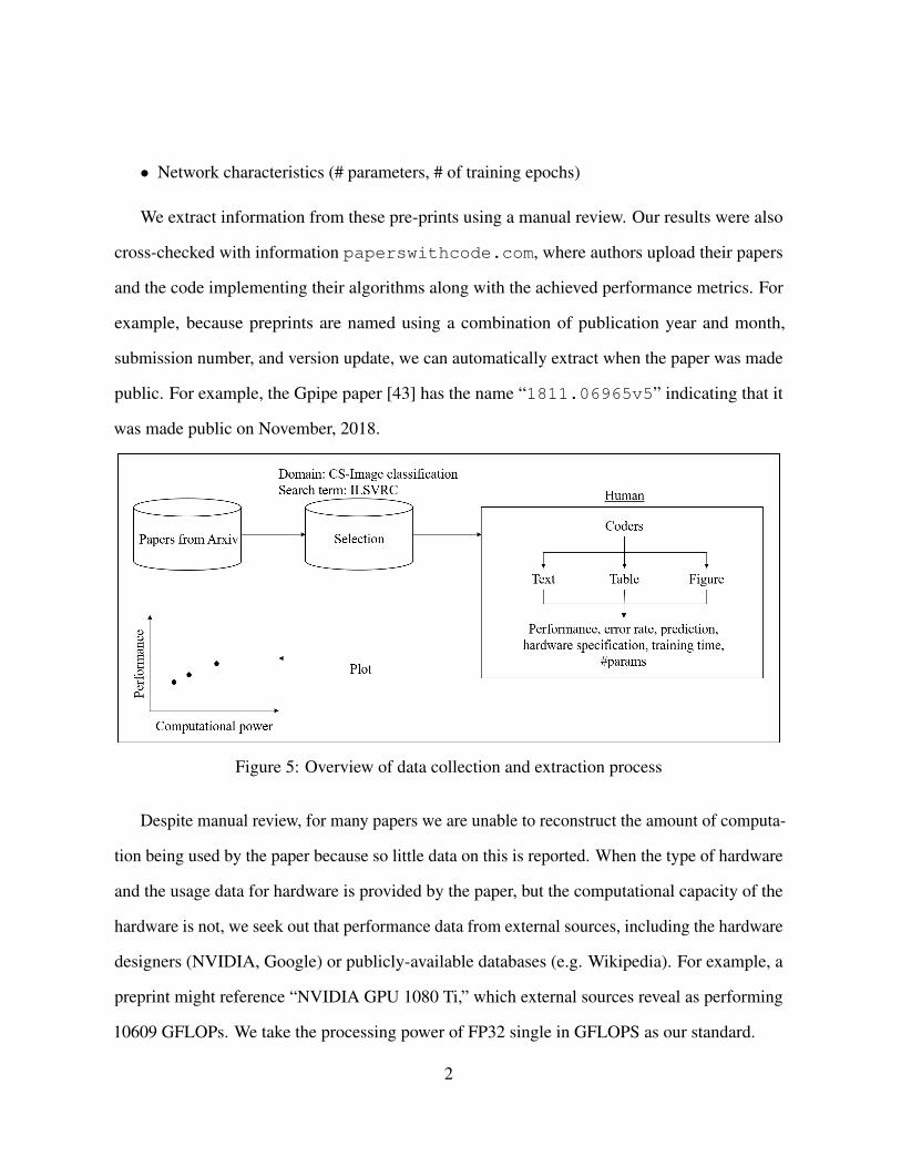
We extract information from these pre-prints using a manual review. Our results were also

cross-checked with information paperswithcode.com, where authors upload their papers

and the code implementing their algorithms along with the achieved performance metrics. For

example, because preprints are named using a combination of publication year and month,

submission number, and version update, we can automatically extract when the paper was made

public. For example, the Gpipe paper [43] has the name “1811.06965v5” indicating that it

was made public on November, 2018.

Figure 5: Overview of data collection and extraction process

Despite manual review, for many papers we are unable to reconstruct the amount of computa-

tion being used by the paper because so little data on this is reported. When the type of hardware

and the usage data for hardware is provided by the paper, but the computational capacity of the

hardware is not, we seek out that performance data from external sources, including the hardware

designers (NVIDIA, Google) or publicly-available databases (e.g. Wikipedia). For example, a

preprint might reference “NVIDIA GPU 1080 Ti,” which external sources reveal as performing

10609 GFLOPs. We take the processing power of FP32 single in GFLOPS as our standard.

2

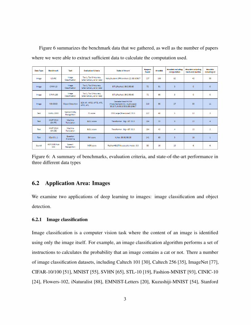
Figure 6 summarizes the benchmark data that we gathered, as well as the number of papers

where we were able to extract sufficient data to calculate the computation used.

Figure 6: A summary of benchmarks, evaluation criteria, and state-of-the-art performance inthree different data types

6.2 Application Area: Images

We examine two applications of deep learning to images: image classification and object

detection.

6.2.1 Image classification

Image classification is a computer vision task where the content of an image is identified

using only the image itself. For example, an image classification algorithm performs a set of

instructions to calculates the probability that an image contains a cat or not. There a number

of image classification datasets, including Caltech 101 [30], Caltech 256 [35], ImageNet [77],

CIFAR-10/100 [51], MNIST [55], SVHN [65], STL-10 [19], Fashion-MNIST [93], CINIC-10

[24], Flowers-102, iNaturalist [88], EMNIST-Letters [20], Kuzushiji-MNIST [54], Stanford

3

Cars [48], and MultiMNIST [28]. We focus on ImageNet and CIFAR-10/100 because their long

history allows us to gather many data points (i.e. papers).

One simple performance measure for image classification is the share of total predictions

for the test set that are correct, called the “average accuracy.” (Or, equivalently, the share that

are incorrect). A common instantiation of this is the “top-k” error rate, which asks whether

the correct label is missing from the top k predictions of the model. Thus, the top-1 error rate

is the fraction of test images for which the correct label is not the top prediction of the model.

Similarly, the top-5 error rate is the fraction of test images for which the correct label is not

among the five predictions.

Benchmark: ImageNet

ImageNet refers to ImageNet Large Scale Visual Recognition Challenge (ILSVRC). It is

a successor of PASCAL Visual Object Classes Challenge (VOC) [29]. ILSVRC provides a

dataset publicly and runs an annual competition as PASCAL VOC. Whereas PASCAL VOC

supplied about 20,000 images labelled as 1 of 20 classes by a small group of annotators, ILSVRC

provides about 1.5M images labelled as 1 of 1000 classes by a large group of annotators. The

ILSVRC2010 dataset contains 1, 261, 406 training images. The minimum number of training

images for a class is 668 and the maximum number is 3047. The dataset also contains 50

validation images and 150 test images for each class. The images are collected from Flickr and

other search engines. Manual labelling is crowdsourced using Amazon Mechanical Turk.

In the ILSVRC2010 competition, instead of deep learning, the winner and the outstanding

team used support vector machines (SVM) with different representation schemes. The NEC-

UIUC team won the competition by using a novel algorithm that combines SIFT [61], LBP [2],

two non-linear coding representations [97, 89], and stochastic SVM [59]. The winning top-5

error rate was 28.2%. The second best performance was done by Xerox Research Centre Europe

(XRCE). XRCE combined an improved Fisher vector representation [68], PCA dimensionality

4

reduction and data compression, and a linear SVM [69], which resulted in top-5 error rate of

33.6%. The trend of developing advanced Fisher vector-based methods continued until 2014.

Deep learning systems begin winning ILSVRC in 2012, starting with the SuperVision team

from University of Toronto which won with AlexNet, achieving a top-5 error rate of 16.4% [52].

Since this victory, the majority of teams submitting to ILSVRCeach year have used deep learning

algorithms.

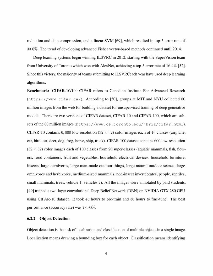
Benchmark: CIFAR-10/100 CIFAR refers to Canadian Institute For Advanced Research

(https://www.cifar.ca/). According to [50], groups at MIT and NYU collected 80

million images from the web for building a dataset for unsupervised training of deep generative

models. There are two versions of CIFAR dataset, CIFAR-10 and CIFAR-100, which are sub-

sets of the 80 million images (https://www.cs.toronto.edu/˜kriz/cifar.html).

CIFAR-10 contains 6, 000 low-resolution (32× 32) color images each of 10 classes (airplane,

car, bird, cat, deer, dog, frog, horse, ship, truck). CIFAR-100 dataset contains 600 low-resolution

(32× 32) color images each of 100 classes from 20 super-classes (aquatic mammals, fish, flow-

ers, food containers, fruit and vegetables, household electrical devices, household furniture,

insects, large carnivores, large man-made outdoor things, large natural outdoor scenes, large

omnivores and herbivores, medium-sized mammals, non-insect invertebrates, people, reptiles,

small mammals, trees, vehicle 1, vehicles 2). All the images were annotated by paid students.

[49] trained a two-layer convolutional Deep Belief Network (DBN) on NVIDIA GTX 280 GPU

using CIFAR-10 dataset. It took 45 hours to pre-train and 36 hours to fine-tune. The best

performance (accuracy rate) was 78.90%.

6.2.2 Object Detection

Object detection is the task of localization and classification of multiple objects in a single image.

Localization means drawing a bounding box for each object. Classification means identifying

5

the object in each bounding box. Localization becomes instance segmentation if, instead of a

bounding box, an object is outlined. Whereas image classification identifies a single object in a

single image, object detection identifies multiple objects in a single image using localization.

There are various performance measures for object detection, all based around the same

concept. Intersection Over Union (IOU) measures the overlap between two bounding boxes: the

ground truth bounding box and the predicted bounding box. This is calculated with a Jaccard

Index, which calculates the similarity between two different sets, A and B, as J(A,B) = |A∩B||A∪B| .

Thus, IOU is the area of the intersection between the two bounding boxes divided by the area of

the union of both two bounding boxes. It is 1 if the ground truth bounding box coincides with

the predicted bounding box.

Box Average Precision (AP), which is also called mean average precision (mAP), sums IOUs

between 0.5 and 0.95 and divides the sum by the number of the IOU values.

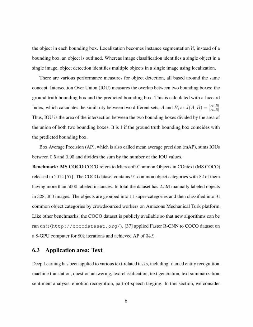
Benchmark: MS COCO COCO refers to Microsoft Common Objects in COntext (MS COCO)

released in 2014 [57]. The COCO dataset contains 91 common object categories with 82 of them

having more than 5000 labeled instances. In total the dataset has 2.5M manually labeled objects

in 328, 000 images. The objects are grouped into 11 super-categories and then classified into 91

common object categories by crowdsourced workers on Amazons Mechanical Turk platform.

Like other benchmarks, the COCO dataset is publicly available so that new algorithms can be

run on it (http://cocodataset.org/). [37] applied Faster R-CNN to COCO dataset on

a 8-GPU computer for 80k iterations and achieved AP of 34.9.

6.3 Application area: Text

Deep Learning has been applied to various text-related tasks, including: named entity recognition,

machine translation, question answering, text classification, text generation, text summarization,

sentiment analysis, emotion recognition, part-of-speech tagging. In this section, we consider

6

three: entity recognition, machine translation, and question answering.

6.3.1 Named Entity Recognition

Named entity recognition is the task of identifying and tagging entities in text with pre-defined

classes (also called “types”). For example, Amazon Comprehend Medical extract relevant

medical information such as medical condition, medication, dosage, strength, and frequency

from unstructured text such as doctors notes [11]. Popular benchmarks are CoNLL 2003,

Ontonotes v5, ACE 2004/2005, GENIA, BC5CDR, SciERC. We focus on CoNLL2003.

Named Entity Recognition is measured using an F1 score, which is the harmonic mean of the

precision and the recall on that task. The precision is the percentage of named entities discovered

by an algorithm that are correct. The recall is the percentage of named entities present in the

corpus that are discovered by the algorithm. Only an exact match is counted in both precision

and recall. The F1 score goes to 1 only if the named entity recognition has perfect precision and

recall, that is, it finds all instances of the classes and nothing else.

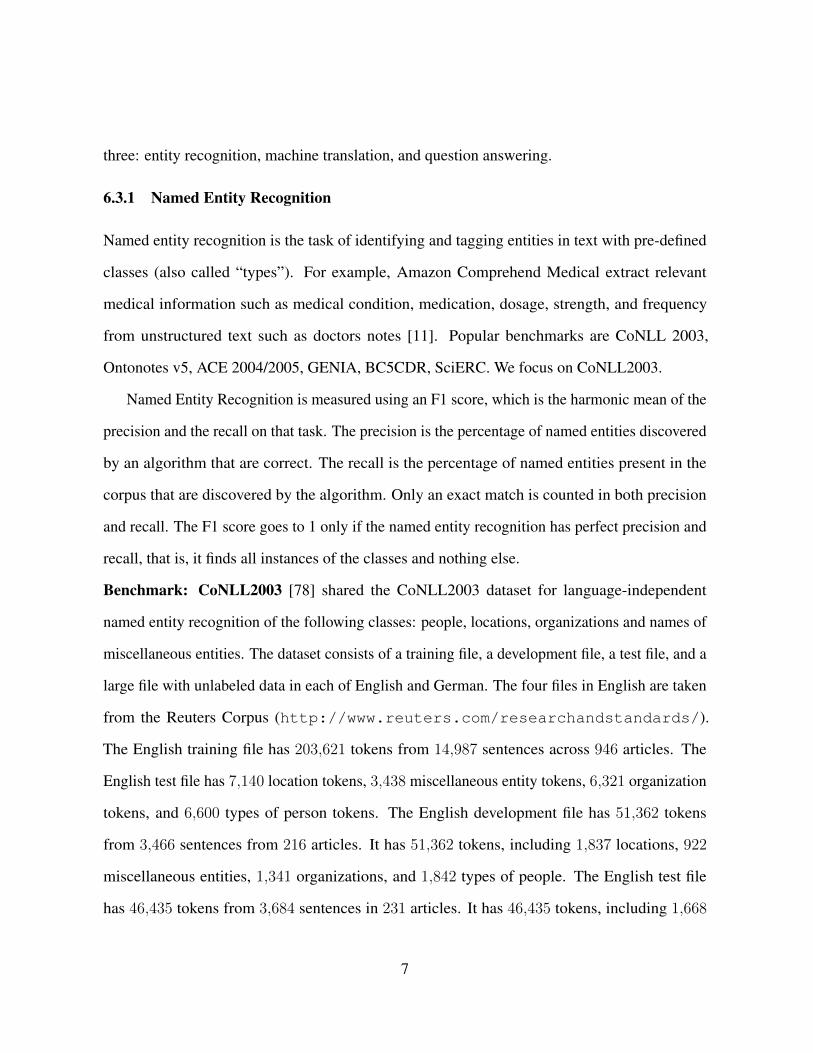
Benchmark: CoNLL2003 [78] shared the CoNLL2003 dataset for language-independent

named entity recognition of the following classes: people, locations, organizations and names of

miscellaneous entities. The dataset consists of a training file, a development file, a test file, and a

large file with unlabeled data in each of English and German. The four files in English are taken

from the Reuters Corpus (http://www.reuters.com/researchandstandards/).

The English training file has 203,621 tokens from 14,987 sentences across 946 articles. The

English test file has 7,140 location tokens, 3,438 miscellaneous entity tokens, 6,321 organization

tokens, and 6,600 types of person tokens. The English development file has 51,362 tokens

from 3,466 sentences from 216 articles. It has 51,362 tokens, including 1,837 locations, 922

miscellaneous entities, 1,341 organizations, and 1,842 types of people. The English test file

has 46,435 tokens from 3,684 sentences in 231 articles. It has 46,435 tokens, including 1,668

7

locations, 702 miscellaneous entities, 1,661 organizations, and 1,617 types of people.

6.3.2 Machine Translation (MT)

MT tasks a machine with translating a sentence in one language to that in a different language.

MT can be viewed as a form of natural language generation from a textual context. MT can

be categorized into rule-based MT, statistical MT, example-based MT, hybrid MT, and neural

MT (i.e., MT based on DL). MT is another task that has enjoyed a high degree of improvement

due to the introduction of DL. Benchmarks are WMT 2014/2016/2018/2019 [12] and IWSLT

2014/2015 [15].

BLEU (Bilingual Evaluation Understudy) [67] score is a metric for translation and computes

the similarity between human translation and machine translation based on n-gram. An n-gram

is a continuous sequence of n items from a given text. The score is based on precision, brevity

penalty, and clipping. The modified n-gram precision means the degree of overlap in n-gram

between reference sentence and translated sentence. Simply, precision is the number of candidate

n-grams which occur in any reference over the total number of n-grams in the candidate. Sentence

brevity penalty is a factor that rescales a high-scoring candidate translation by considering the

extent to match the reference translations in length, in word choice, and in word order. It is

computed by a decaying exponential in the test corpus effective reference length (r) over the

total length of the candidate translation corpus (c), rc. Hence the brevity penalty is 1 if c exceeds

r and exp(1− rc) otherwise.

BLEU is a multiplication of an exponential brevity penalty factor and the geometric mean of

the modified n-gram precisions after case folding, as the equation below.

BLEU = min{1, e(1−r/c)} × e(∑N

n=1 wn log pn).

Here, N is the maximum number that n can have. wn is a weight on n-gram. pn is the modified

n-gram precision.

8

BLEU score ranges from 0 to 1. 1 is the best possible score but is only achieved when a

translation is identical to a reference translation. Thus even a human translator may not reach 1.

BLEU has two advantages. First, it can be applied to any language. Second, it is easy and quick

to compute. BLEU is known to have high correlation with human judgments by computing the

average of individual sentence judgment errors over a test corpus.

Benchmark: WMT2014 WMT‘14 contains 4.5M sentence pairs (116M English words and

110M German words) as training data (https://www.statmt.org/wmt14/translation-task.

html).

6.3.3 Question Answering (QA)

QA is a task of machine to generate a correct answer to a question from an unstructured collection

of documents in a certain natural language. QA requires reading comprehension ability. Reading

comprehension of a machine is to understand natural language and to comprehend knowledge

about the world.

Benchmarks include but are not limited to Stanford Question Answering Dataset (SQuAD),

WikiQA, CNN, Quora Question Pairs, Narrative QA, TrecQA, Childrens Book Test, TriviaQA,

NewsQA, YahooCQA.

F1 score and Exact Match (EM) are popular performance measures. EM measures the

percentage of predictions that match any one of the ground truth answers exactly. The human

performance is known to be 82.304 for EM and 91.221 for F1 score.

Benchmark: SQuAD1.1 SQuAD consists of questions posted by crowd workers on a set of

Wikipedia articles. And the answer to every question may be in a segment of text. SQuAD1.1

contains 107,785 question-answer pairs on 536 articles [74]. [74] collected question-answer

pairs by crowdsourcing using curated passages in top 10,000 articles of English Wikipedia from

Project Nayukis Wikipedias internal PageRanks. Plus, the authors collected additional answers

9

to the questions that have crowdsourced answers already.

The dataset is available here (https://worksheets.cdalab.org/worksheets/

0xd53d03a48ef64b329c16b9baf0f99b0c/).

6.4 Application area: Sound6.4.1 Speech recognition

Speech recognition is the task of recognizing speech within audio and converting it into the

corresponding text. The first part of recognizing speech within audio is performed by an acoustic

model and the second part of converting recognized speech into the corresponding text is done

by a language model [46]. The traditional approach is to use Hidden Markov Models (HMMs)

and Gaussian Mixture Models (GMMs) for acoustic modeling in speech recognition. Artificial

neural networks (ANNs) were applied to speech recognition since the 1980s. ANNs empowered

the traditional approach from the end of 20th century [41]. Recently, DL models such as CNNs

and RNNs improved the performance of acoustic models and language models, respectively.

More recently, end-to-end automatic speech recognition based on CTC (Connectionist Temporal

Classification) [33, 34] has been growing in popularity. Baidu’s DeepSpeech2 [4] and Googles

LAS (Listen, Attend and Spell) [16] are examples. Speech recognition also requires large scale

high quality datasets in order to improve performance.

One simple way to measure the performance of speech recognition is to compare the body

of text read by a speaker with the transcription written by a listener. And, WER (Word Error

Rate) is a popular metric of the performance of a speech recognition. It is difficult to measure the

performance of speech recognition because the recognized word sequence can have a different

length from the reference word sequence. WER is based on Levenshtein distance in word level.

In addition, dynamic string alignment is utilized to cope with the problem of the difference

in word sequence lengths. WER can be computed by dividing the sum of the number of

10

substitutions, the number of deletions, the number of insertions by the number words in a

reference sequence. Namely, the corresponding accuracy can be calculated by subtracting WER

from 1. The exemplary benchmarks are Switchboard, LibriSpeech, TIMIT, and WSJ.

Benchmark: ASR SWB Hub500 Automatic Speech Recognition Switchboard Hub 500 (ASR

SWB Hub500) dataset contains 240 hours of English telephone conversations collected by Lin-

guistic Data Consortium (LDC) [21] (https://catalog.ldc.upenn.edu/LDC2002S09).

7 Model Analysis

7.1 Computations per network pass

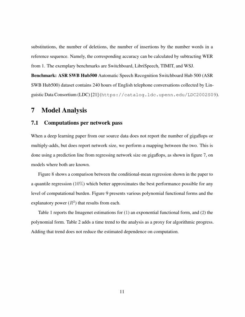
When a deep learning paper from our source data does not report the number of gigaflops or

multiply-adds, but does report network size, we perform a mapping between the two. This is

done using a prediction line from regressing network size on gigaflops, as shown in figure 7, on

models where both are known.

Figure 8 shows a comparison between the conditional-mean regression shown in the paper to

a quantile regression (10%) which better approximates the best performance possible for any

level of computational burden. Figure 9 presents various polynomial functional forms and the

explanatory power (R2) that results from each.

Table 1 reports the Imagenet estimations for (1) an exponential functional form, and (2) the

polynomial form. Table 2 adds a time trend to the analysis as a proxy for algorithmic progress.

Adding that trend does not reduce the estimated dependence on computation.

11

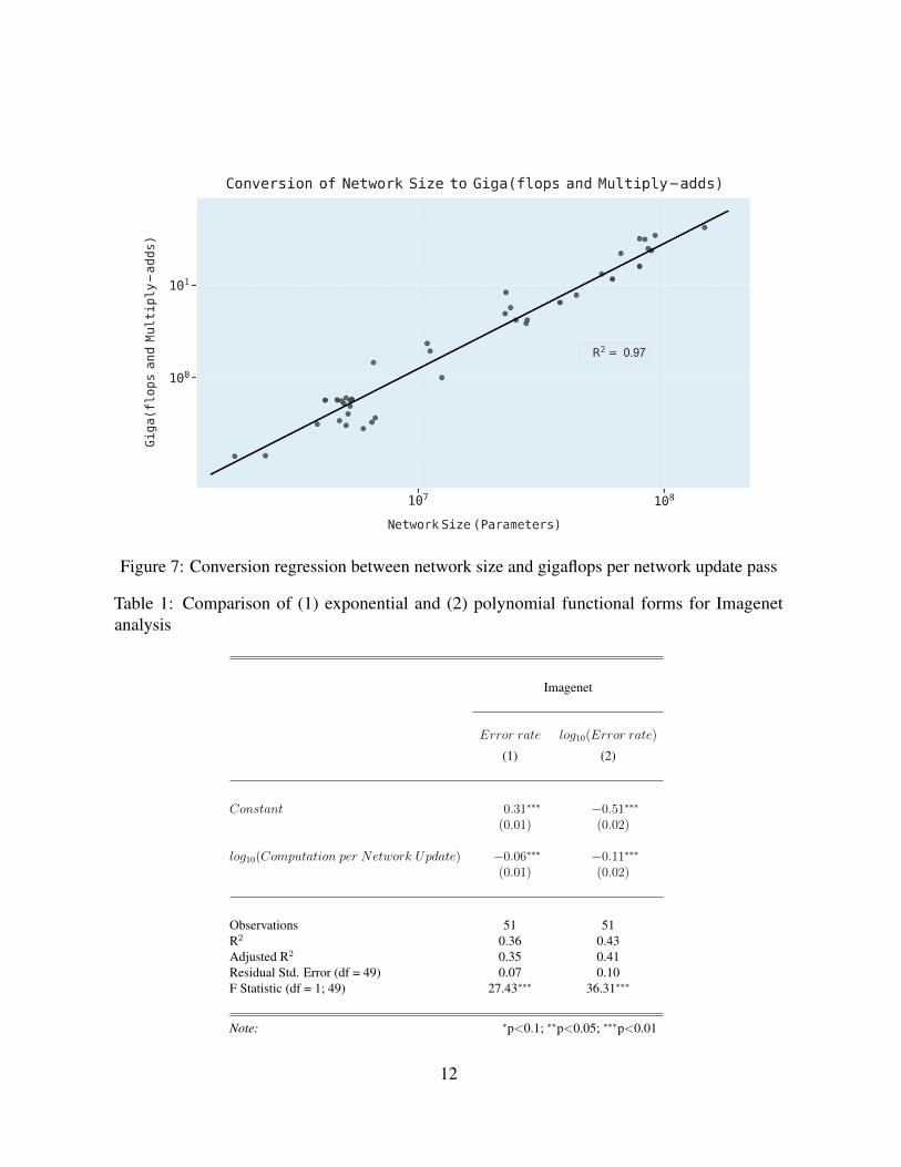
Figure 7: Conversion regression between network size and gigaflops per network update pass

Table 1: Comparison of (1) exponential and (2) polynomial functional forms for Imagenetanalysis

Imagenet

Error rate log10(Error rate)

(1) (2)

Constant 0.31∗∗∗ −0.51∗∗∗(0.01) (0.02)

log10(Computation per Network Update) −0.06∗∗∗ −0.11∗∗∗(0.01) (0.02)

Observations 51 51R2 0.36 0.43Adjusted R2 0.35 0.41Residual Std. Error (df = 49) 0.07 0.10F Statistic (df = 1; 49) 27.43∗∗∗ 36.31∗∗∗

Note: ∗p<0.1; ∗∗p<0.05; ∗∗∗p<0.01

12

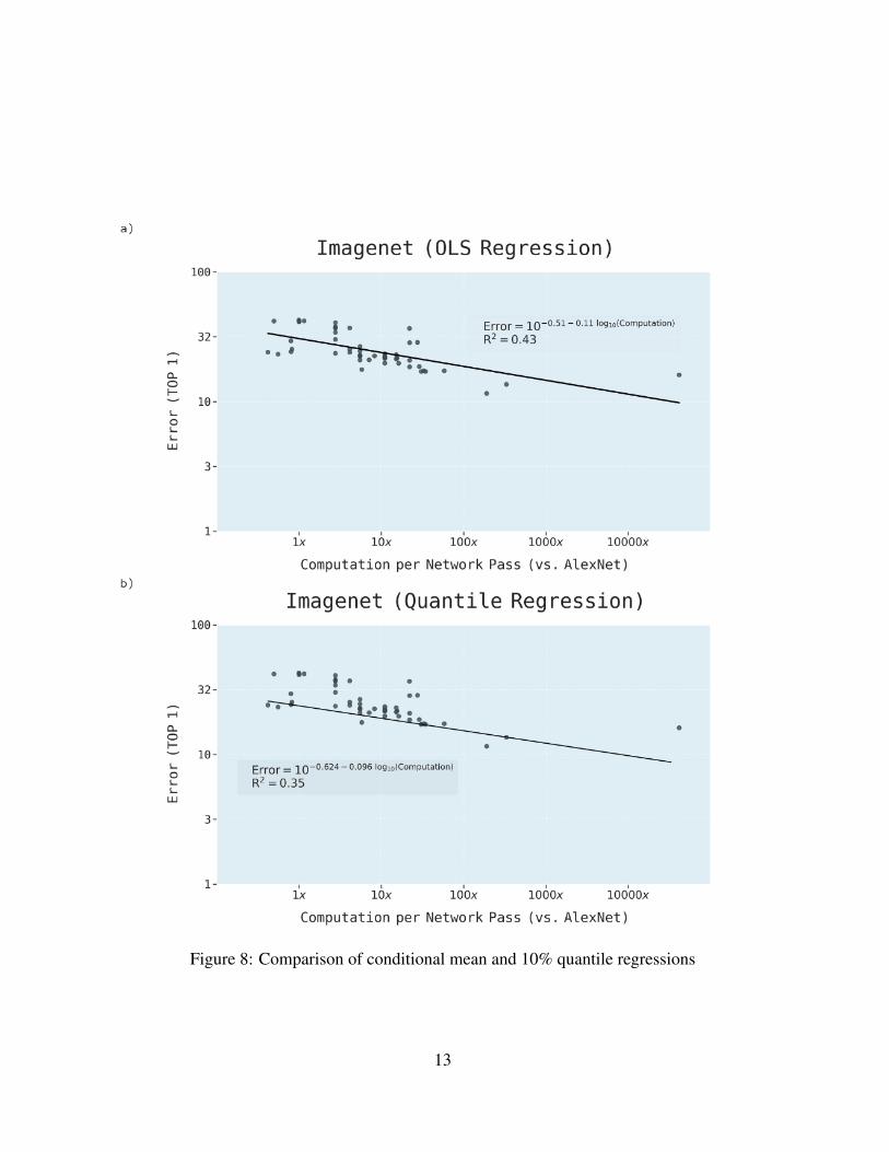
Figure 8: Comparison of conditional mean and 10% quantile regressions

13

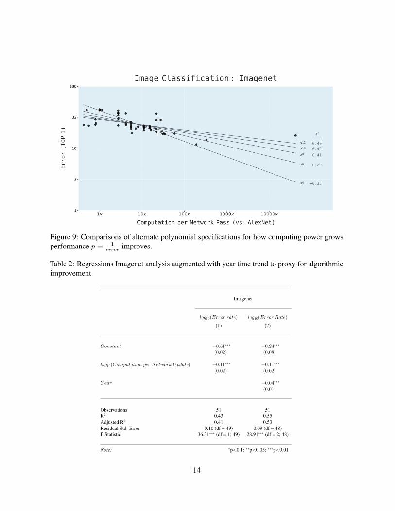
Figure 9: Comparisons of alternate polynomial specifications for how computing power growsperformance p = 1

errorimproves.

Table 2: Regressions Imagenet analysis augmented with year time trend to proxy for algorithmicimprovement

Imagenet

log10(Error rate) log10(Error Rate)

(1) (2)

Constant −0.51∗∗∗ −0.24∗∗∗(0.02) (0.08)

log10(Computation per Network Update) −0.11∗∗∗ −0.11∗∗∗(0.02) (0.02)

Y ear −0.04∗∗∗(0.01)

Observations 51 51R2 0.43 0.55Adjusted R2 0.41 0.53Residual Std. Error 0.10 (df = 49) 0.09 (df = 48)F Statistic 36.31∗∗∗ (df = 1; 49) 28.91∗∗∗ (df = 2; 48)

Note: ∗p<0.1; ∗∗p<0.05; ∗∗∗p<0.01

14

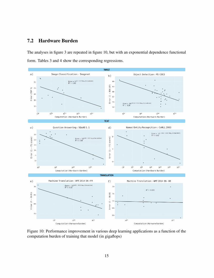
7.2 Hardware Burden

The analyses in figure 3 are repeated in figure 10, but with an exponential dependence functional

form. Tables 3 and 4 show the corresponding regressions.

Figure 10: Performance improvement in various deep learning applications as a function of thecomputation burden of training that model (in gigaflops)

15

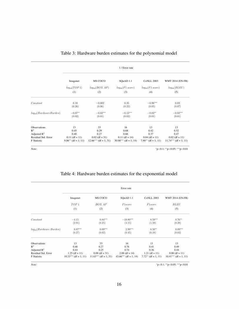
Table 3: Hardware burden estimates for the polynomial model

1 / Error rate

Imagenet MS COCO SQuAD 1.1 CoNLL 2003 WMT 2014 (EN-FR)

log10(TOP 1) log10(BOX AP ) log10(F1 score) log10(F1 score) log10(BLEU)

(1) (2) (3) (4) (5)

Constant 0.10 −0.002 0.35 −0.96∗∗∗ 0.03(0.26) (0.06) (0.22) (0.05) (0.07)

log10(HardwareBurden) −0.07∗∗ −0.02∗∗∗ −0.13∗∗∗ −0.02∗∗ −0.02∗∗∗(0.02) (0.01) (0.02) (0.01) (0.01)

Observations 13 33 16 13 13R2 0.45 0.29 0.68 0.42 0.52Adjusted R2 0.40 0.27 0.66 0.37 0.47Residual Std. Error 0.11 (df = 11) 0.02 (df = 31) 0.11 (df = 14) 0.04 (df = 11) 0.02 (df = 11)F Statistic 9.06∗∗ (df = 1; 11) 12.66∗∗∗ (df = 1; 31) 30.00∗∗∗ (df = 1; 14) 7.90∗∗ (df = 1; 11) 11.74∗∗∗ (df = 1; 11)

Note: ∗p<0.1; ∗∗p<0.05; ∗∗∗p<0.01

Table 4: Hardware burden estimates for the exponential model

Error rate

Imagenet MS COCO SQuAD 1.1 CoNLL 2003 WMT 2014 (EN-FR)

TOP 1 BOX AP F1score F1score BLEU

(1) (2) (3) (4) (5)

Constant −4.15 0.84∗∗∗ −19.80∗∗∗ 8.59∗∗∗ 0.76∗∗

(2.91) (0.25) (4.15) (1.59) (0.28)

log10(Hardware Burden) 0.87∗∗∗ 0.09∗∗∗ 2.99∗∗∗ 0.50∗∗ 0.09∗∗∗

(0.27) (0.02) (0.45) (0.18) (0.03)

Observations 13 33 16 13 13R2 0.48 0.27 0.76 0.41 0.49Adjusted R2 0.44 0.25 0.74 0.36 0.44Residual Std. Error 1.25 (df = 11) 0.08 (df = 31) 2.08 (df = 14) 1.21 (df = 11) 0.08 (df = 11)F Statistic 10.33∗∗∗ (df = 1; 11) 11.63∗∗∗ (df = 1; 31) 43.66∗∗∗ (df = 1; 14) 7.72∗∗ (df = 1; 11) 10.41∗∗∗ (df = 1; 11)

Note: ∗p<0.1; ∗∗p<0.05; ∗∗∗p<0.01

16