The Complete Transmission Spectrum of WASP-39b with a Precise Water Constraint

H. R. Wakeford1,2 , D. K. Sing1 , D. Deming3, N. K. Lewis2,4 , J. Goyal1, T. J. Wilson1, J. Barstow5 , T. Kataria6 ,B. Drummond1 , T. M. Evans1 , A. L. Carter1, N. Nikolov1, H. A. Knutson7, G. E. Ballester8, and A. M. Mandell9

1 Astrophysics Group, University of Exeter, Physics Building, Stocker Road, Devon, EX4 4QL, UK; stellarplanet@gmail.com2 Space Telescope Science Institute, 3700 San Martin Drive, Baltimore, MD 21218, USA

3 Department of Astronomy, University of Maryland, College Park, MD 20742, USA4 Department of Earth and Planetary Sciences, Johns Hopkins University, Baltimore, MD 21218, USA

5 University College London, London, UK6 NASA Jet Propulsion Laboratory, 4800 Oak Grove Drive, Pasadena, CA 91109, USA

7 Division of Geological and Planetary Sciences, California Institute of Technology, Pasadena, CA 91125, USA8 Lunar and Planetary Laboratory, University of Arizona, Tucson, AZ 85721, USA

9 NASA Goddard Space Flight Center, Greenbelt, MD 20771, USAReceived 2017 September 18; revised 2017 November 24; accepted 2017 November 27; published 2017 December 21

Abstract

WASP-39b is a hot Saturn-mass exoplanet with a predicted clear atmosphere based on observations in the opticaland infrared. Here, we complete the transmission spectrum of the atmosphere with observations in the near-infrared(NIR) over three water absorption features with the Hubble Space Telescope (HST) Wide Field Camera 3 (WFC3)G102 (0.8–1.1 μm) and G141 (1.1–1.7 μm) spectroscopic grisms. We measure the predicted high-amplitude H2Ofeature centered at 1.4 μm and the smaller amplitude features at 0.95 and 1.2 μm, with a maximum waterabsorption amplitude of 2.4 planetary scale heights. We incorporate these new NIR measurements into previouslypublished observational measurements to complete the transmission spectrum from 0.3 to 5 μm. From theseobserved water features, combined with features in the optical and IR, we retrieve a well constrained temperatureTeq=1030 20

30-+ K, and atmospheric metallicity 151 46

48´-+ solar, which is relatively high with respect to the currently

established mass–metallicity trends. This new measurement in the Saturn-mass range hints at further diversity inthe planet formation process relative to our solar system giants.

Key words: planets and satellites: atmospheres – planets and satellites: individual (WASP-39b) –techniques: spectroscopic

1. Introduction

Exoplanets have greatly advanced our understanding ofplanetary systems, expanding theory and observations beyondour solar system (e.g., Fortney et al. 2010; Seager & Deming2010; Deming et al. 2013; Marley et al. 2013; Stevensonet al. 2014; Evans et al. 2016; Kataria et al. 2016; Sing et al.2016; Deming & Seager 2017). Due to remote observingtechniques, close-in giant planets dominate atmosphericcharacterization studies, in part because of their large planet-to-star radius ratios, but mostly due to large extendedatmospheres, which scatter and transmit a greater number ofphotons. Observations using transmission spectroscopy havemeasured atomic (Na and K) and molecular (H2O) absorptionin a range of exoplanet atmospheres with ground- and space-based telescopes (e.g., Charbonneau et al. 2002; Singet al. 2011, 2015; Deming et al. 2013; Kreidberg et al. 2014;Stevenson et al. 2014; Evans et al. 2016; Nikolov et al. 2016;Sing et al. 2016). While water has been detected in a number ofexoplanet atmospheres, precise and constraining measurementsof H2O absorption are still rare (e.g., Kreidberg et al. 2014;Wakeford et al. 2017).

Observational data analysis is a non-trivial exercise and thereare an array of techniques being applied to reduce data (e.g.,Berta et al. 2012; Gibson et al. 2012; Deming et al. 2013;Wakeford et al. 2016). In a comparative observational study of10 hot-Jupiter exoplanets using the Hubble and Spitzer SpaceTelescopes with consistent data analysis techniques, Sing et al.(2016) present a startling diversity in atmospheric transmissionspectral features, where clouds play a significant role mutingand obscuring atomic and molecular absorption features. Sing

et al. (2016) defined a transmission spectral index as a means todistinguish between cloudy and clear atmospheres using theamplitude of water absorption observed with Hubble SpaceTelescope (HST) Wide Field Camera 3 (WFC3) versus thealtitude difference between optical wavelengths, measured withSpace Telescope Imaging Spectrograph (STIS), and IRwavelengths, measured with Spitzer Space Telescope InfraredArray Camera (IRAC). The transmission spectral indexeffectively displayed trends in the “clarity” of an exoplanetatmosphere with a continuum from clear to cloudy for the 10planets in the study. One of the planets in this study is thehighly inflated Saturn-mass planet WASP-39b.WASP-39b has a radius of 1.27 RJ and a mass of just 0.28MJ

and is in orbit around a late G-type star with a period of 4.055days (Faedi et al. 2011). Out of current well-characterizedexoplanets, only the hot Jupiters WASP-31b and WASP-17bhave lower bulk densities (Anderson et al. 2010, 2011; Singet al. 2016). However, both are more massive and moreirradiated than WASP-39b, which has a lower equilibriumtemperature of 1116 K. Analysis of STIS data in the optical andSpitzer/IRAC data in the IR shows a spectrum consistent witha predominately clear atmosphere based on both forward modeland retrieval studies (Sing et al. 2016; Barstow et al. 2017). Thestrongest evidence of a clear atmosphere from the currentobservational data of WASP-39b is the presence of a strong Nafeature in the transmission spectrum with pressure-broadenedline wings for both Na and K absorption lines (Fischeret al. 2016; Nikolov et al. 2016). These alkali features would bemuted or obscured if clouds were present and would not extendto the H/He continuum. Near-infrared (NIR) features, on the

The Astronomical Journal, 155:29 (14pp), 2018 January https://doi.org/10.3847/1538-3881/aa9e4e© 2017. The American Astronomical Society. All rights reserved.

1

other hand, would be less sensitive to these clouds, given theinherent wavelength dependence of light scattered by smallparticles (Bohren & Huffman 2008). At the time of the Singet al. (2016) study, no NIR HST/WFC3 observations existedfor WASP-39b, and the atmospheric water absorption could notbe measured. Therefore, the “clarity” of the atmosphere (i.e.,the transmission spectral index) could not be calculated. In thispaper, we present three transit observations of WASP-39busing WFC3 from 0.8 to 1.7 μm and place precise constraintson the water content in the atmosphere of the planet andcalculate a definitive transmission spectral index. In Section 2,we detail the analysis of the new observations in the NIR. Wethen present the complete transmission spectrum of WASP-39bfrom 0.3 to 5 μm in Section 3 and introduce the theoreticalmodels used to interpret this data set. We detail the retrievedatmospheric parameters in Section 4 and discuss the implica-tions these have on the nature of WASP-39b with respect totemperature, metallicity, and chemical abundances, as well asplanetary formation.

2. WFC3 Observations and Analysis

We observed WASP-39b during three transit events usingHST WFC3 G102 grism as part of GO-14169 (PI. Wakeford)on 2016 July 7, and WFC3 G141 grism as part of GO-14260(PI. Deming) on 2016 August 29 and 2017 February 7.Observations for both spectroscopic grisms were conducted inforward spatial scan mode. Spatial scanning involves exposingthe telescope during a forward slew in the cross-dispersiondirection and resetting the telescope position to the top of thescan prior to conducting subsequent exposures. Scans withG102 were conducted at a scan rate of ∼0.26 pixels per secondwith a final scan covering ∼28 pixels in the cross-dispersiondirection. For G141, we used a scan rate of ∼0.30 pixels persecond with a final spatial scan covering ∼44 pixels in thecross-dispersion direction on the detector (Figure 1).

We use the IMA output files from the CalWF3 pipeline,which are calibrated using flat fielding and bias subtraction.We extract the spectrum from each exposure by taking thedifference between successive non-destructive reads. A top-hatfilter (Evans et al. 2016) is then applied around the targetspectrum and all external pixels are set to zero to aid the

removal of cosmic rays (Nikolov et al. 2015). The imageis then reconstructed by adding the individual reads backtogether. We then extract the stellar spectrum from eachexposure with an aperture of±14 pixels for G102 and±22 pixels for G141 around a centering profile, which wasfound to be consistent across the spectrum for each exposurefor each observation.We monitored each transit with HST over the course of five

orbits with observations occurring before, during, and aftertransit. We discard the first orbit of each visit, as it containsvastly different systematics to the subsequent orbits (e.g.,Deming et al. 2013; Kreidberg et al. 2015; Sing et al. 2016;Wakeford et al. 2016, 2017). This is due to thermal settlingrequired after target acquisition, which results in a differentthermal pattern for the telescope not replicated in subsequentorbits.

2.1. White Light Curve

We first analyze the band-integrated light curves of WASP-39 to obtain the broad-band planet-to-star radius ratio (Rp/R*),by summing the flux between 0.8 and 1.13 μm for G102 andbetween 1.12 and 1.66 μm for G141. The uncertainties on eachdata point were initially set to pipeline values dominated byphoton and readout noise. We account for stellar limbdarkening using a four-parameter limb-darkening law(Claret 2000; Sing 2010). Each light curve is fit using theIDL routine MPFIT, which uses a Lavenberg–Markwardt(L–M) least-squares algorithm (Markwardt 2012), which hasbeen shown to produce posterior distributions that are welldescribed by a multi-variable Gaussian distribution (e.g., Singet al. 2016; Wakeford et al. 2016, 2017). After an initial fit, theuncertainties on each time series exposure are rescaled basedon the standard deviation of the residuals, taking into accountany underestimated uncertainties calculated by the reductionpipeline in the data points. The final uncertainty for each pointis then determined from the covariance matrix from the L–Malgorithm. We fix the system parameters to the previouslyestablished values: inclination=87.36°, a R*=11.043, per-iod=4.055259 days (Nikolov et al. 2016). From the band-integrated light curve, we fit for the center of transit time andfix it for subsequent spectroscopic light curves.We use marginalization across a series of systematic models to

account for observatory- and instrument-based systematics(Gibson 2014). As detailed in Wakeford et al. (2016), we use agrid of polynomial models, which approximates stochasticmodels, to account for established systematic trends. Eachsystematic models accounts for up to three detrending parameters;θ, f, and dl, where θ accounts for a linear increase/decrease offlux in time across the whole observation, f is the HST orbitalphase trends based on the thermal “breathing” of the telescopeover the course of each orbit around the Earth, and dl is the shift inwavelength position of the spectrum caused by telescope pointing.We use combinations with and without θ, and with or without fand dl, up to the 4th order. This results in a grid of 50 systematicmodels that we test against our data, where the most complex hasthe following function:

S t T p l, . 1i

n

ii

j

n

jj

11 1

å ål q f d= ´ ´ l= =

( ) ( )

Here, T1, pi, and lj are fit variables or fixed to zero if unfit in aspecific model (see Wakeford et al. 2016 for a table all

Figure 1. “IMA” image files of WASP-39 from each visit. The top row showsthe direct image taken of the target star with the WFC3 F139M filter, which isused for wavelength calibration of the spectroscopic trace. The bottom rowshows the first exposure of each visit: from left to right we show the G102grism trace, G141 visit 1 trace, and G141 visit 2 trace. Each of the independentobservational parameters are listed on the figures.

2

The Astronomical Journal, 155:29 (14pp), 2018 January Wakeford et al.

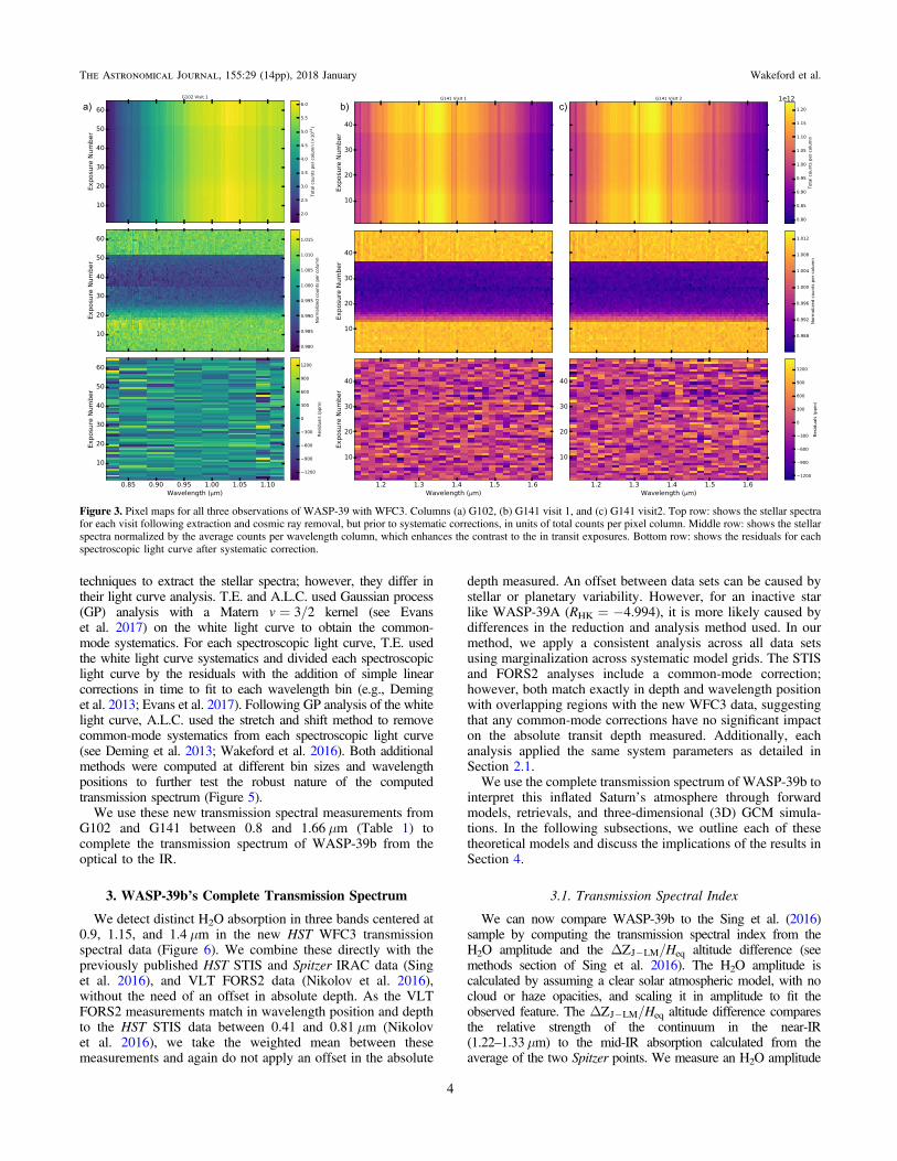
parameter combinations). It is important to note that margin-alization relies on the fact that at least one of the models beingmarginalized over is a good representation of the systematics inthe data. Marginalizing over a series of models then allows forgreater flexibility in satisfying this condition, over the use of asingle systematic model. We use the maximum likelihoodestimation based on the Akaike Information Criterion (AIC) toapproximate the evidence-based weight for each systematicmodel (Burnham & Anderson 2004). While the AIC is anapproximation to the evidence, it allows for more flexiblemodels to be folded into the likelihood, as compared to theBayesian Information Criterion (BIC), which typically leads tomore conservative error estimates on the marginalized values(Gibson 2014; Wakeford et al. 2016). We marginalize acrossall systematic models to compute the desired light curveparameters. Using marginalization across a large grid of modelsallows us to account for all tested combinations of systematicsand obtain robust center of transit times from the band-integrated light curve, and transit depths for each spectroscopiclight curve. We measure a center of transit time of2457577.425837±0.000044 (JDUTC) for the G102 visit,2457630.149461±0.000044 (JDUTC) for visit 1 with G141,and 2457792.356338±0.000041 (JDUTC) for visit 2 withG141. We show the white light curves for each visit in Figure 2along with the highest weighted model from our analysis andthe marginalized broad-band transit depth in terms of R Rp *.To demonstrate the noise properties of the data, we show thepixel maps of the stellar spectra following spectral extraction,cosmic ray corrections, and wavelength alignment (Figure 3) inboth total counts (top) and in normalized counts (middle). Thebottom panel of Figure 3 shows the residuals from eachspectroscopic light curve, the analysis of which is outlined inthe following section. These plots demonstrate that there are noobvious bad pixels in these data, and no wavelength-dependenttrends in the spectroscopic light curves.

2.2. Spectroscopic Light Curves

We divide the WFC3 wavelength range of each grism into aseries of bins and measure the Rp/R* from each spectroscopiclight curve (Table 1) following the same procedure as detailedfor the band-integrated light curve. For each visit, we test arange of bin widths and wavelength ranges. For G102, we testbin widths from lD =0.0146–0.0490 μm over wavelengthranges of 0.8–1.12 μm and 0.81–1.13 μm. For G141, we testbins of lD =0.0186, 0.0128, 0.0373, and 0.0467 μm, overtwo wavelength ranges (1.12–1.65 μm 1.13–1.66 μm). Foreach bin and wavelength range, we find that the shape of thetransmission spectrum is robust and consistent.For the presented transmission spectrum, we divide the G102

spectroscopic range into eight bins between 0.81 and 1.13 μmwith variable bin sizes of lD =0.0244 or 0.0490 μm (Table 1).For each spectroscopic light curve, we test all 50 models andmarginalize over the transit parameters to compute the Rp/R*. Wefind that there are few wavelength-dependent systematics asevidenced by the similarity between the highest weightedsystematic model for each spectroscopic light curve fit.For the G141 grism observations, we extract and analyze

each visit separately. As with the band-integrated analysis, wemarginalize over all systematic models to compute the transitparameters. For both G141 visits, we use 28 equal bin sizes oflD =0.0186 μm between 1.13 and 1.66 μm (Table 1). We

found both transmission spectra using the G141 grism to beconsistent in absolute depth (Figure 4). We then combine theminto a single spectrum by taking the weighted mean of eachspectroscopic measurement (Table 1).To determine if the analysis method used is justified, we

compute the transmission spectrum from each visit using adifferent analysis pipeline (Evans et al. 2016) over multiple binsizes (T. Evans (T.E.): lD =0.0500 μm, A.L. Carter (A.L.C.):lD =0.0186μm) and compute the weighted mean spectrum.

We find that the different methods result in the same transmissionspectrum in shape and absolute depth within the 1σ uncertainties(Figure 5). The additional analyses performed used similar

Figure 2. White light curves of the WASP-39b transit in each visit. Top: the raw (colored) and corrected (black) light curves with the best-fit model (solid line).Middle top: dl which is the positional shift on the detector between each exposure spectrum. Middle bottom: raw residuals and uncertainties (colored points), with thebest-fit systematic model (solid lines). Bottom: corrected light curve residuals (black points). (a) G102, (b) G141 visit 1, (c) G141 visit 2.

3

The Astronomical Journal, 155:29 (14pp), 2018 January Wakeford et al.

techniques to extract the stellar spectra; however, they differ intheir light curve analysis. T.E. and A.L.C. used Gaussian process(GP) analysis with a Matern v=3/2 kernel (see Evanset al. 2017) on the white light curve to obtain the common-mode systematics. For each spectroscopic light curve, T.E. usedthe white light curve systematics and divided each spectroscopiclight curve by the residuals with the addition of simple linearcorrections in time to fit to each wavelength bin (e.g., Deminget al. 2013; Evans et al. 2017). Following GP analysis of the whitelight curve, A.L.C. used the stretch and shift method to removecommon-mode systematics from each spectroscopic light curve(see Deming et al. 2013; Wakeford et al. 2016). Both additionalmethods were computed at different bin sizes and wavelengthpositions to further test the robust nature of the computedtransmission spectrum (Figure 5).

We use these new transmission spectral measurements fromG102 and G141 between 0.8 and 1.66 μm (Table 1) tocomplete the transmission spectrum of WASP-39b from theoptical to the IR.

3. WASP-39b’s Complete Transmission Spectrum

We detect distinct H2O absorption in three bands centered at0.9, 1.15, and 1.4 μm in the new HST WFC3 transmissionspectral data (Figure 6). We combine these directly with thepreviously published HST STIS and SpitzerIRAC data (Singet al. 2016), and VLT FORS2 data (Nikolov et al. 2016),without the need of an offset in absolute depth. As the VLTFORS2 measurements match in wavelength position and depthto the HST STIS data between 0.41 and 0.81 μm (Nikolovet al. 2016), we take the weighted mean between thesemeasurements and again do not apply an offset in the absolute

depth measured. An offset between data sets can be caused bystellar or planetary variability. However, for an inactive starlike WASP-39A (RHK=−4.994), it is more likely caused bydifferences in the reduction and analysis method used. In ourmethod, we apply a consistent analysis across all data setsusing marginalization across systematic model grids. The STISand FORS2 analyses include a common-mode correction;however, both match exactly in depth and wavelength positionwith overlapping regions with the new WFC3 data, suggestingthat any common-mode corrections have no significant impacton the absolute transit depth measured. Additionally, eachanalysis applied the same system parameters as detailed inSection 2.1.We use the complete transmission spectrum of WASP-39b to

interpret this inflated Saturn’s atmosphere through forwardmodels, retrievals, and three-dimensional (3D) GCM simula-tions. In the following subsections, we outline each of thesetheoretical models and discuss the implications of the results inSection 4.

3.1. Transmission Spectral Index

We can now compare WASP-39b to the Sing et al. (2016)sample by computing the transmission spectral index from theH2O amplitude and the ΔZJ LM- /Heq altitude difference (seemethods section of Sing et al. 2016). The H2O amplitude iscalculated by assuming a clear solar atmospheric model, with nocloud or haze opacities, and scaling it in amplitude to fit theobserved feature. The ΔZJ LM- /Heq altitude difference comparesthe relative strength of the continuum in the near-IR(1.22–1.33μm) to the mid-IR absorption calculated from theaverage of the two Spitzerpoints. We measure an H2O amplitude

Figure 3. Pixel maps for all three observations of WASP-39 with WFC3. Columns (a) G102, (b) G141 visit 1, and (c) G141 visit2. Top row: shows the stellar spectrafor each visit following extraction and cosmic ray removal, but prior to systematic corrections, in units of total counts per pixel column. Middle row: shows the stellarspectra normalized by the average counts per wavelength column, which enhances the contrast to the in transit exposures. Bottom row: shows the residuals for eachspectroscopic light curve after systematic correction.

4

The Astronomical Journal, 155:29 (14pp), 2018 January Wakeford et al.

of 37%±7% withΔZJ LM- /Heq=−0.09±0.35 (see Figure 7).A near-zero altitude difference and relatively low water amplitudeplaces WASP-39b further away from the clear solar abundancemodel, although this does not change its position in the clear tocloudy continuum displayed in Sing et al. (2016) as compared tothe other nine exoplanets in the study. While this index showsthat the water amplitude is less than expected for a completelyclear solar abundance atmosphere, each of these model tracksvaries only a single parameter, with all others held fixed; in reality,each of these parameters will vary simultaneously. Additionally,previous observations and theoretical models of extrasolar gasgiant planets show that these planets may have metallicities greaterthan 1× solar (e.g., Kreidberg et al. 2014; Thorngren et al. 2016;Wakeford et al. 2017). We comment further on this planet’smetallicity in Section 4.5.

3.2. Goyal Forward Model Grid

We use the newly developed open source grid of forwardmodel transmission spectra produced using the one-dimensional(1D) radiative-convective equilibrium model ATMO (Amundsen

et al. 2014; Tremblin et al. 2015, 2016; Drummond et al. 2016)outlined in Goyal et al. (2017), to compare to our measuredtransmission spectrum. Each model assumes isothermal pressure–temperature (P–T) profiles and equilibrium chemistry with rainoutcondensation. It includes multi-gas Rayleigh scattering and high-temperature opacities due to H2O, CO2, CO, CH4, NH3, Na, K,Li, Rb, Cs, TiO, VO, FeH, PH3, H2S, HCN, C2H2, SO2, as wellas H2–H2, H2–He collision-induced absorption (CIA). The gridconsists of 6272 model transmission spectra specifically forWASP-39b (i.e., with gravity, Rp, etc. of WASP-39b), whichexplores a combination of eight temperatures (516 K, 666K,741 K, 816 K, 966 K, 1116K, 1266 K, and 1416 K), sevenmetallicities (0.005, 0.1, 1, 10, 50, 100, 200× solar), seven C/Ovalues (0.15, 0.35, 0.56, 0.70, 0.75, 1.0, and 1.5), four “haze”parameters (1, 10, 150, and 1100), and four cloud parameters(0, 0.06, 0.2, and 1). In the Goyal grid, the “haze” parameterdefines an enhanced Rayleigh-like scattering profile, whichincreases the hydrogen cross section with a wavelength-dependentprofile. The “cloud” parameter defines a gray uniform scatteringprofile across all wavelengths between 0% and 100% cloudopacity (see Goyal et al. 2017 for more details).We fit each model to the transmission spectrum by only

allowing them to move in absolute altitude; we therefore haveone free parameter for each model fit. We use the L–M routineMPFIT to determine the best-fit altitude and calculate the 2c .

Table 1Marginalized Transmission Spectrum of WASP-39B Measured with HST

WFC3 G102 and G141 Grism

λ lD Rp/R*Uncertainty

(μm) (μm) (ppm)

G1020.8225 0.0244 0.14435 3100.8592 0.0490 0.14482 1900.9082 0.0490 0.14539 1400.9572 0.0490 0.14598 1501.0062 0.0490 0.14541 1301.0552 0.0490 0.14457 1501.0920 0.0244 0.14475 2201.1165 0.0244 0.14596 240

G1411.1391 0.0186 0.14567 7101.1578 0.0186 0.14625 4101.1765 0.0186 0.14611 4301.1951 0.0186 0.14542 5801.2138 0.0186 0.14500 6801.2325 0.0186 0.14536 5101.2512 0.0186 0.14576 6401.2699 0.0186 0.14417 4001.2885 0.0186 0.14628 7601.3072 0.0186 0.14582 6021.3259 0.0186 0.14663 5151.3446 0.0186 0.14663 4691.3633 0.0186 0.14687 6601.3819 0.0186 0.14733 5801.4006 0.0186 0.14749 5921.4193 0.0186 0.14674 5001.4380 0.0186 0.14788 6501.4567 0.0186 0.14772 7581.4753 0.0186 0.14803 6331.4940 0.0186 0.14718 6771.5127 0.0186 0.14653 6701.5314 0.0186 0.14655 7211.5501 0.0186 0.14656 5181.5687 0.0186 0.14607 6771.5874 0.0186 0.14519 7111.6061 0.0186 0.14588 6711.6248 0.0186 0.14596 8401.6435 0.0186 0.14441 614

Figure 4. WFC3 transmission spectrum measured over three visits with G102and G141 grisms. The measured transmission spectrum from the G102 visitfrom 0.8 to 1.12 μm is shown in light blue circles. We analyzed the two visitswith G141 separately and show each transmission spectrum (visit 1 triangles,visit 2 downward triangles), and the transmission spectrum computed from theaverage of the separate spectra (dark red circles). The G141 spectrum iscomputed from 1.12 to 1.66 μm with a constant bin width oflD =0.0186 μm.

Figure 5. Comparison of the average transmission spectrum computed for theG141 visits based on three different analyses.

5

The Astronomical Journal, 155:29 (14pp), 2018 January Wakeford et al.

We transform from 2c to probability likelihood via theexpression

x xp A exp12

, 22c= -⎜ ⎟⎛⎝

⎞⎠( ) ( ) ( )

where x T , M H , C O, H, Cº { [ ] } are the temperature,metallicity, carbon-to-oxygen ratio, haze, and cloud para-meters, respectively, and A is a normalization constant. Thisconstant is set by integrating the likelihood over all modelparameters, such that

x xp d 1. 3ò ò =" ( ) ( )

The Goyal grid is specifically generated for each planet and therange of each of the parameters are reasonable assumptions for

a planetary atmosphere. As such, we assume a weaklyinformative prior on each model, which is uniform to the edgeof the grid space where it is truncated.We fit the model grid to both the full transmission spectrum

(0.3–5 μm) and a subset containing only the new WFC3 data(0.8–1.7 μm). The probability distribution of the model grid isshown in Figure 8 for both scenarios. We then select the modelwith the highest probability for each data set and plot them inFigure 9 against the complete transmission spectrum of WASP-39b. From these plots, we see a distinct difference between thebest-fit temperature and haze parameters with just the H2Ofeatures, and with the full optical and NIR transmissionspectrum. These differences predominantly impact the opticalportion of the spectrum, which anchors the haze parameter butis largely degenerate with the temperature. Additionally, thehaze and cloud parameters have a widespread influence on the

Figure 6. The complete transmission spectrum of WASP-39b (black points). This transmission spectrum incorporates data from HST STIS and WFC3, SpitzerIRAC,and VLT FORS2 completing the spectrum from 0.3 to 5.0 μm with currently available instruments. Using the ATMO retrieval code, which implements an isothermalprofile and equilibrium chemistry, we determine the best-fit atmospheric model (red) and show the 1, 2, and 3σ confidence regions (dark to light blue) based on theretrieved parameters.

Figure 8. Probability distribution of the forward model grid fit to the data forthe new WFC3 results only (purple) and the full transmission spectrumincluding STIS, VLT, and Spitzerpoints (green). These pairs plots show thecorrelations between the five parameters explored in the model grid with therespective probability histograms for each parameter.

Figure 7. Transmission spectral index diagram of ΔZJ LM- vs. H2O amplitudeas defined in Sing et al. (2016). Black points show the altitude differencebetween the NIR and IR spectral features (ΔZJ LM- ) vs. the H2O amplitudemeasured at 1.4 μm, each with 1σ errorbars. Purple and gray lines show themodel trends for haze and clouds, respectively. Red shows the trend for sub-and super-solar metallicities. Green shows the model trend for different C/O.

6

The Astronomical Journal, 155:29 (14pp), 2018 January Wakeford et al.

C/O and metallicity, which is further highlighted by theinclusion of the optical and IR data. We discuss this further inSection 4.

3.3. ATMO Retrieval

We use the ATMO Retrieval Code (ARC) to fully explorethe parameter space covered by the transmission spectralmeasurements. Using ARC, we calculate the posteriordistribution of the data to the models and determine the fitconfidence intervals marginalizing over parameter space (seeWakeford et al. 2017 and Evans et al. 2017 for further details).ARC couples the ATMO model to an L–M least-squaresminimizer and a Differential Evolution Chain Monte Carlo(DECMC) analysis (Eastman et al. 2013). We ran DECMCswith 12 chains each with 30000 steps, with convergencetypically occurring around 15000 steps, where convergence ismonitored using the Gelman–Rubin statistic. We consideredtwo atmospheric retrieval models: a chemically consistentretrieval scheme that assumes chemical equilibrium and a moreflexible free-chemistry retrieval. In the equilibrium chemistryretrieval, the chemical abundances are consistent with the P–Tprofile. In the free-chemistry retrieval, the abundances areassumed to be constant with pressure and are independently fit.For the opacity sources, we include H2–H2, H2–He CIA, andmolecular opacities from H2O, CO, CO2, CH4, NH3, Na, andK. For both models, we assume isothermal P–T profiles.Parameterized P–T profiles were explored, although found tobe unnecessary to fit the data, as the retrieved P–T profiles werefound to be isothermal over the altitudes probed by the datawith no significant structure in the P–T profile indicated by thefit parameters.

In each retrieval, we fit for a haze and cloud parameter, eachof which are scaling factors applied to the hydrogen crosssection with either a wavelength-dependent profile (haze) oruniform profile (cloud)—these two parameters are representedin ARC (Figure 10) as a natural log ratio for numerical reasonsonly. Using the equilibrium retrieval, we also run a fit to onlythe new WFC3 data, as with the Goyal grid, to determine theimpact of the optical and IR transmission spectrum in theretrieved parameters.

In Table 2, we list the main results from the ARC analysis,with each model having the following free parameters,respectively.

Equilibrium: planetary radius (Rp), Teq, Haze, Cloud,[M/H], C/O.

Free-chemistry: Rp, Teq, Haze, Cloud, H2O volume mixingratio (VMR), CO2 VMR, CO VMR, CH4 VMR, Na VMR, andK VMR.From this retrieval, we are able to place constraints on the

equilibrium temperature of the observed portion of theplanetary atmosphere, as well as the C/O and metallicity byfitting the absorption features. In the equilibrium chemistrycase, the abundance of elemental carbon and oxygen species isset via the C/O and metallicity. Specifically in ATMO, thecarbon abundance is set as a multiple of the solar carbon (C)abundance

A AC C, solar 10 , 4M H= ´( ) ( ) ( )[ ]

and then the oxygen (O) abundance is set via the carbonabundance and the CO ratio

A AO C CO . 5ratio=( ) ( ) ( )In the free-chemistry model, each species abundance is fitindependently, and [M/H] is estimated based on the H2Oabundance. The C/O ratio is then estimated from the four fitmolecules containing carbon and/or oxygen (CO, CO2, CH4,H2O) and does not take into account any other species. The Naand K line profiles are modeled using an Allard profile (Allardet al. 2007); alternate profiles were tested but did not improveupon the statistical fit to the data.We find that the data are described best with an isothermal

equilibrium model that has a 2cn of 1.32 compared to 1.45 forthe free-chemistry fit. From this, we retrieve Teq=1030 20

30-+

and an atmospheric metallicity 151 4648´-

+ solar, as defined by theposterior distributions (Figure 10).

3.4. 3D GCM

To model the 3D temperature structure of WASP-39b, weuse the SPARC/MITgcm (Showman et al. 2009). TheSPARC/MITgcm couples the MITgcm, a finite-volume codethat solves the 3D primitive equations on a staggered ArakawaC grid (Adcroft et al. 2004) with a two-stream adaptation of amulti-stream radiative transfer code for solar system planets(Marley & McKay 1999). The radiative transfer code employs

Figure 10. Probability density map of the ARC fit to the data for the the fulltransmission spectrum, using equilibrium chemistry and an isothermal P–Tprofile. These pairs plots show the correlations between the six parametersexplored in the ARC DECMC with the respective probability densityhistograms for each parameter.

Figure 9. Highest probability grid models fit to the the transmission spectrumfor, the new WFC3 results only (purple) and the full transmission spectrum(green) including STIS, VLT, and Spitzerpoints.

7

The Astronomical Journal, 155:29 (14pp), 2018 January Wakeford et al.

the correlated-k method with 11 bands optimized for accuracyand computational efficiency. The opacities are calculatedassuming local thermodynamic and chemical equilibrium. Thiscode has been used extensively to model the atmosphericcirculation of exoplanets (e.g., Lewis et al. 2010; Kataria et al.2015, 2016; Lewis et al. 2017; Wakeford et al. 2017).

Here, we show the P–T profiles from Kataria et al. (2016) forWASP-39b averaged over different regions of the atmosphere,demonstrating the impact of 3D circulation on the planetaryP–T profiles (Figure 11(a)). We also plot the retrievedtemperature based on isothermal equilibrium models at thepressure probed by these observations. Also shown are thecondensation curves of potential cloud species in the atmos-phere of WASP-39b, as well as the molecular transition regionfrom CO-dominated carbon chemistry to CH4-dominatedcarbon chemistry. From the 3D GCM, we derive a condensa-tion map showing the average temperature as a function oflongitude and pressure indicating where and what condensatesmight form in the atmosphere (Figure 11(b)). The GCM resultssuggest that the two limbs of the planet likely have differentcloud properties due to the recirculation of heat around theplanet from the dayside hemisphere. The nightside trailing limb(west) is approximately 100 K colder than the Sun trailinglimb (east) at pressures of 0.1 bar, and up to 200 K colder atpressures less than 1 mbar. These differences in the limbs notonly influence the average temperature observed in transmis-sion, but also in this case will impact the condensate cloudspecies likely to form in the atmosphere on the colder westernlimb. This becomes important when considering the impactdifferences in the limbs will have on the transmission spectrum,which measures the average absorption profile of the limbannulus around the planet (e.g., Line et al. 2016).

We note that this model is for a 1× solar composition caseand with an increased atmospheric metallicity, the temperatureis likely to increase as well as the position of the condensationcurves (Wakeford et al. 2017). Additionally, there is evidencethat the day–night temperature contrast will also change (likelyincrease) with metallicity (Kataria et al. 2014; Charnayet al. 2015, B. Drummond et al. 2017, in preparation), whichwould have consequences on the east–west limb cloudformation.

4. Discussion

We present the complete transmission spectrum of WASP-39b from 0.3 to 5.0 μm combining data from HST STISand WFC3, VLT FORS2, and SpitzerIRAC. Figure 6 showsthe absorption features of WASP-39b’s atmosphere, which

includes broad sodium line wings and three distinct waterabsorption peaks. There is also tentative evidence of absorptionby potassium in the optical and absorption due to carbon-basedspecies in the Spitzer4.5 μm channel.In our analysis, we find that the data are described best with

an isothermal equilibrium model with Teq=1030 2030

-+ and

[M/H]=151 4648´-

+ solar. At the 1σ level, WASP-39b has someof the most constrained atmospheric parameters to date. In thissection, we discuss the implications from the interpretivemethods used and the importance of the complete transmissionspectrum.

4.1. Forward Models and Retrievals

To interpret the transmission spectrum of WASP-39b, weused a grid of 6272 forward models that were specificallycalculated for WASP-39b (Goyal et al. 2017). The Goyal gridsamples five different atmospheric parameters commonlyexplored in a retrieval code; temperature, metallicity, C/O,scattering haze, and uniform clouds. Based on results from theGoyal grid, we find that the data are best described by a highmetallicity (100× solar), low C/O (0.15), hazy (150×)atmosphere (Figure 9). The large sampling of models in thegrid allows for more detailed interpretation compared to takinga handful of non-specific exoplanet models, with the additionthat the probability distributions can be explored. The gridprobability distributions suggest that uniform clouds are notplaying a significant role in the observed transmissionspectrum, where any cloud parameter applied to the data isequally probable given a distribution of the other fourparameters (Figure 8). As there are no carbon-bearing speciesin the transmission spectrum of WASP-39b, the C/O ratio isconstrained to the lowest value in the grid. This makes it moredifficult to statistically infer precise atmospheric values as thetail end of the distributions are being cut (c.f. Goyalet al. 2017).Using the ARC, we implement an isothermal equilibrium

chemistry model and expand upon the parameter space coveredby the Goyal grid. While the grid contains sparse sampling ofall five parameters, the ARC uses DECMC to thoroughlyexplore tens of thousands of models. From both the Goyal gridand ARC, we find hard cut-offs in the temperature space; this islikely due to the inclusion of the optical data and the presenceof sodium absorption in the observed spectrum, whichcondenses in the models for lower temperatures (seeSection 4.3). In the Goyal grid, the temperature cut-off appearsat 966 K, while the finer sampling used in the ARC leads to amore accurate cut-off of ∼1000 K. Below this temperature,

Table 2Results from Each Retrieval Model

Data Model k DOF 2c BIC Teq M/H C/O H2O Na KChemistry (K) (log10) [VMR] [VMR] [VMR]

×solar ×Solar ×Solar ×Solar

WFC3 Equilib. 5 31 31.9 49.8 950 150130

-+ 1.88 0.65

0.41-+ 0.19 0.16

0.29-+ L L L

76 59117

-+

Full Equilib. 5 65 88.1 109.0 1030 2030

-+ 2.18 0.16

0.12-+ 0.31 0.05

0.08-+ L L L

151 4648

-+

Full Free- 10 60 85.8 128.3 920 6070

-+ 2.07 0.13

0.05-+ 0.44 0.44

0.11-+ −1.37 0.13

0.05-+ −3.7 0.6

0.6-+ −4.9 1.3

0.8-+

Chem. 117 3014

-+ 117 30

14-+ 120 90

330-+ 105 100

620-+

Note. [VMR] is log10(Volume Mixing Ratio).

8

The Astronomical Journal, 155:29 (14pp), 2018 January Wakeford et al.

significant amounts of rainout removes Na from the gas phase,which condenses into Na2S and/or NaAlSi3O8.

Using ARC, we can further explore the distribution of C/Oand metallicity. While these parameters are highly correlated,ARC is able to explore the limits of the distribution withC/O< 0.15, and [M/H]> 2.7. Interestingly, increased sam-pling on the cloud parameter yields no further interpretation.One advantage of using the Goyal grid over ARC is speed—thefit to the entire Goyal grid can be run in minutes, while a fullretrieval with ARC can take many days. From our analysis, wecan see that the Goyal grid is able to constrain planetaryparameters within reasonable limits as described by thecurrent data.

4.2. Interpreting the Chemistry

Using ARC, we run both an equilibrium chemistry modeland a free-chemistry model to fit for chemical species andabundances in the measured atmosphere (see Section 3.3). BothATMO chemistry models retrieve similar parameters fortemperature, metallicity, and C/O (Table 2). The high-resolution and precision of data over the 0.9, 1.2, and 1.4 μmwater absorption features place good constraints on thetemperature and metallicity retrieved by each model. Theseare further reinforced in the free-chemistry fit by the individualabundances retrieved for the Na and K absorption features inthe optical, which have similar VMR to the H2O, and thereforeinform the overall atmospheric metallicity. The presence of Nain the transmission spectrum also informs the temperature ofthe atmosphere, as at low temperatures (<1000 K) Na wouldlikely be depleted by rainout, confining it deeper in theatmosphere. The thermosphere of an exoplanet is mostsensitively probed by the Na line core (e.g., Huitsonet al. 2012). However, the line core of Na is not resolved inthe transmission spectrum of WASP-39b, which prohibits amore detailed investigation of the line core and the inclusion of

the thermosphere in the models detailed. In the case that theNa line core temperature is underestimated, the model will notbe able to match the data higher in the atmosphere (Figures 6and 9). To further constrain the temperature and structure ofWASP-39bs thermosphere, high-resolution observations of Nawill be required.Following the results from the solar-metallicity GCM of

WASP-39b (Figure 11), we might expect to observe absorptionby CH4 in the atmosphere of WASP-39b, as a number of theP–T profiles cross the CO=CH4 boundary. However, we donot see any evidence for methane absorption in the transmis-sion spectrum, which would be present at the red end of theG141 bandpass (>1.55 μm) and in the 3.6 μm Spitzerband-pass. Both the equilibrium chemistry and free-chemistryretrievals suggest that the atmosphere of WASP-39b likelyhas a metallicity greater than 100× solar. The high metallicitywill impact not only the P–T profiles by pushing them to highertemperatures but would also push the CO=CH4 transition tolower temperatures, particularly at high pressures (Agúndezet al. 2014). This likely places the atmosphere of WASP-39b

Figure 11. (a) 1× solar 3D P–T profiles of WASP-39b. The global, dayside, nightside, limb, east, and west limb averaged profiles computed from 3D GCM models ofWASP-39b (see Kataria et al. 2016). Also plotted are the condensation curves of the affecting species, as well as the CO/CH4 abundance line. These P–T profilesindicate a difference in temperature expected on opposite limbs of the planet, resulting in the potential for one limb to be observationally clear while the other containsmore significant cloud opacities. The point indicates the temperature retrieved for the atmosphere of WASP-39b based on an isothermal equilibrium model (Table 2).(b) Average temperature of WASP-39b as a function of longitude and pressure. Temperatures are weighted by the cosine of the latitude, equivalent to weighting eachgrid point by its projection angle toward an observer at the equator. Low-temperature condensates are overplotted in this 2D space.

Figure 12. The transmission spectrum of WASP-39b (black points). We showthe result from both ATMO retrievals using equilibrium chemistry (green) andfree chemistry (orange) with the 1, 2, and 3σ bounds as in Figure 6.

9

The Astronomical Journal, 155:29 (14pp), 2018 January Wakeford et al.

firmly above the CO=CH4 boundary, in the CO-dominatedregime, for all pressures and all locations horizontally. It istherefore not likely that the CH4 abundance is enhancedrelative to equilibrium abundances due to horizontal or verticalquenching, as has been postulated for many hot-Jupiteratmospheres (e.g., Cooper & Showman 2006; Agúndezet al. 2014).

The only current evidence of carbon-based species in thetransmission spectrum of WASP-39b is in the 4.5 μmSpitzerbandpass, which covers potential absorption by COand/or CO2. In Figure 12, we show the difference in retrievedmodels from the equilibrium and free-chemistry cases. Fromthis, we can see that the equilibrium chemistry model strugglesto fit the data, as the fit is likely dominated by the high-precision transmission spectrum below 1.7 μm. In the free-chemistry model, because all the molecules are individually fit,the CO/CO2 can be balanced such that each molecules is fit bythe model. However, this results in much larger uncertaintieson the data as wider distributions are invoked to account forlow-resolution data. The CO feature also extends slightlybeyond the photometric wavelength range covered by theSpitzerpoint, which also extends the uncertainty of the model.Due to the high metallicity of the atmosphere, the 4.5 μmfeature is likely dominated by CO2 absorption (Moseset al. 2013). Future observations with James Webb SpaceTelescope (JWST) will be able to better distinguish betweencarbon-based species in the atmosphere and it is then likely thefree-chemistry model will provide a more informative retrieval.However, with the current data and based on the 2cn and BIC,the equilibrium model has the greatest statistical significance;as such we use this model and results to further interpret theatmosphere of WASP-39b.

4.3. The Importance of the Optical Data in ConstrainingMolecular Abundances

We next explored the impact different wavelength regionshave on the overall metallicity constraint by performing anidentical equilibrium retrieval, but excluding the optical HSTand VLT data below 0.8 μm. Optical transmission spectra havebeen theoretically shown to be important when measuring theVMR of species (Benneke & Seager 2012; Griffith 2014; Line& Parmentier 2016; Heng & Kitzmann 2017), as an infrared-only transmission spectra provides only the relative abundances

between molecules. However, few demonstrations are availableusing optical spectral data. While similar data are available forother exoplanets (Sing et al. 2016), this test is particularlyenlightening with WASP-39b, as it has continuous wavelengthcoverage from 0.3 to 1.7 μm thanks to the WFC3/G102 data.This complete coverage includes pressure-broadened alkalilines (Fischer et al. 2016), multiple well-resolved waterfeatures, and overall higher quality data (precision andresolution) than many other exoplanetary spectra.We use equilibrium chemistry models to compare the

retrieved results for the full and partial WASP-39b data, as itprovided the best overall fit to the data as measured by the BIC.The results can be seen in Figure 13. Despite adopting chemicalequilibrium and including the Spitzer IRAC data in theretrieval, the infrared-only data was unable to constrain thelower end of the C/O ratio, and a very strong degeneracy wasobserved between the C/O and [M/H]. Without the opticaldata, the 3σ range of the transmission spectra at 0.3 μmencompasses 3.4 pressure scale heights (Figure 13 purplerange) and contains a wide range of models, including oneswith a strong haze, completely cloud- or haze-free models, andmodels with both near solar and highly super-solar metallicity(see Figure 13). The posterior of the infrared-only retrievalshows the [M/H] is measured to 0.64 dex; however, a lowerprior value of 0.01 was enforced on the C/O ratio which, inturn, also limits the lower range of [M/H]. By including theoptical HST and VLT data into the retrieval, pressureinformation from the alkali lines and constraints on the near-UV scattering slope help to limit the parameter space and[M/H], which in turn helps constrain the C/O ratio as well.Even though the near-UV transmission spectral features can notuniquely be pinned to Rayleigh scattering of the bulk H2 gas, asa scattering aerosol contribution is also present and included inthe retrieval model, the optical data does exclude models witheither very high or very low haze components, which helps toconstrain the fitted parameters. With the optical data, theresulting [M/H] is measured to 0.14 dex, which is a 0.5 deximprovement over excluding the optical data. The abundanceconstraints of water (as determined by the [M/H] and C/Oratio see Section 3.3) are also significantly improved fromprecisions of±86× to±46× solar.From this test, we demonstrate that the optical spectra with

the data quality as provided by HST and VLT can provide animportant contribution in constraining the abundances of

Figure 13. Left: histograms showing the relative frequency distributions for each parameter (Temperature, [M/H], C/O, Rp/R*, Haze, and Cloud) in the equilibriumretrieval for the full data set (green) and just the IR portion of the data set (purple). Right: the complete transmission spectrum of WASP-39b (black points), where theIR data is indicated by purple points. The two models show equilibrium models fit to the full transmission spectrum (green), and just the IR points (purple), with the 1,2, and 3σ bounds. These clearly show the uncertainty associated with limited wavelength coverage and the importance of the optical.

10

The Astronomical Journal, 155:29 (14pp), 2018 January Wakeford et al.

molecules identified from infrared transmission spectra. In theabsence of optical data, breaking the [M/H]–C/O degeneracywill likely require complete near-infrared spectral coverage toidentify all the major molecular components (CO, CO2, CH4,H2O) such that the C/O ratio can be directly measured and inturn [M/H] constrained (Greene et al. 2016). For JWST,coverage between 0.6 and 5 μm for targets brighter than J∼10will require at least two transit observations (e.g., NIRISS/SOSS and NIRSpec/G395H), while fainter targets can coverthe range at low resolution in one transit with the NIRSpecprism. Given that significant O and C could be locked up inother species such as condensates (Greene et al. 2016), theinclusion of optical data may also prove useful to identifypotential biases when estimating the C/O ratio solely from themajor molecular components. Thus, significant leverage can begained by combining JWST spectra with that of HST or otherground-based facilities, though care must always be takenwhen interpreting non-simultaneously gathered data, especiallyif the planet orbits an active star.

4.4. The Impact of Limb Differences

Overall, the retrieved temperature matches well with the 3DGCM model, where increases in the metallicity would shift theP–T profiles hotter (Figure 11). At higher temperatures, itmight then be expected that the difference in temperature at thetwo limbs will also increase (Kataria et al. 2016). Differences inlimb temperatures may result in different conditions at the eastand west limbs of the annulus such that cloud condensates canform at one and not the other (see Figure 11).

The presence of clouds on one limb of the planet but not theother can potentially mimic high metallicity signatures in the

transmission spectrum (Line & Parmentier 2016). Using thesimplistic toy model presented in Line & Parmentier (2016),which uses a linear combination of two forward models toapproximate limb differences, we test the scenario that the twolimbs are different with a series of models on the fulltransmission spectrum of WASP-39b. We use a range of 1Disothermal models from the Goyal grid to represent differentatmospheric scenarios on the planetary limbs. Using Figure 11as a guide, we select two models separated by 200 K, where thecooler model (741 K) represents the fully cloudy limb (i.e., auniform optically thick cloud across all wavelengths), and thehotter model (966 K) represents the clear, cloud-free limb. Foreach model set, we keep the C/O, [M/H], and haze parametersthe same. We test six sets with varied [M/H] values of 0.0, 1.7,and 2.0 dex (1×, 50×, and 100× solar). For each of the threemetallicities, we then test two different haze values, 10× and150× (Table 3). We fit each separate model to the WASP-39btransmission spectrum by allowing it to move in altitude only,with all other parameters considered fixed. In effect, this onlyintroduces one free parameter to the fit; however, it should benoted that the models themselves while fixed are based on anumber of variables, which, when modeled more comprehen-sively to determine limb differences, may impact the statisticsof fit to the data. The ΔBIC values presented in Table 3represent the difference in BIC between the best-fit model andall other models in the table. From this test, we find that thehigher metallicity models statistically fit the data better thanlow metallicity cases, even when 50/50 clear/cloudy modelsare considered. However, it should be noted that this is anoversimplified parameter space being explored. Future obser-vations of WASP-39b, which will likely have completewavelength coverage and much higher precision and resolutiondata, will likely require sophisticated 3D modeling toaccurately infer anything further from the data when consider-ing partly cloudy scenarios.These simple toy model results, along with the abundance

measurements from equilibrium and free-chemistry retrievals,further suggest that WASP-39b has a high metallicityatmosphere. We detail the implications of this in the followingsection.

4.5. The Atmospheric Metallicity of WASP-39b

There are two scenarios generally considered for theformation of giant planets prior to the assumed migration ofclose-in giant exoplanets: gravitational instability and coreaccretion. Planetary atmospheres will exhibit different atmo-spheric properties under formation via these two formationpathways. Gravitational instability theory suggests that planetswill have the same atmospheric metallicity as the central star,while with core accretion theory, lower-mass planets will havehigher atmospheric metallicity (e.g., Mordasini et al. 2012;Fortney et al. 2013). Studies of our solar system giant planetsfit with the predicted trend of core accretion when theatmospheric methane abundance is used as a proxy for overallmetallicity (c.f Kreidberg et al. 2014). More recently, atmo-spheric water absorption features in exoplanet atmosphereshave been used with retrieval modeling to constrain the overallatmospheric metallicity using oxygen as a proxy for the heavyelement abundance (Fraine et al. 2014; Kreidberg et al. 2014,2015; Wakeford et al. 2017). The first measurement of this typewas conducted on WASP-43b (Kreidberg et al. 2014), whichdirectly fit with the trend established by the solar system

Table 3Test Cases for the Impact of Limb Differences on the Observed

Transmission Spectrum

Group Teq [M/H] Haze Cloud 2c BIC ΔBIC(K)

(a) 741 0.0 10.0 1.0 196 200 50966 0.0 10.0 0.0 327 331 181

50/50 L L L L 179 187 37

(b) 741 0.0 150.0 1.0 360 364 214966 0.0 150.0 0.0 757 762 612

50/50 L L L L 514 522 372

(c) 741 1.7 10.0 1.0 149 153 3966 1.7 10.0 0.0 326 330 180

50/50 L L L L 166 174 24

(d) 741 1.7 150.0 1.0 180 184 34966 1.7 150.0 0.0 224 228 78

50/50 L L L L 174 182 32

(e) 741 2.0 10.0 1.0 157 161 11966 2.0 10.0 0.0 224 228 78

50/50 L L L L 142 150 0

(f) 741 2.0 150.0 1.0 175 178 28966 2.0 150.0 0.0 158 162 12

50/50 L L L L 146 154 2

Note. In each pair, the two models contribute 50% each to the combinedmodel. Each model and the combined model are fit to the transmissionspectrum and the 2c , BIC, and ΔBIC (compared to the lowest BIC model) arecalculated (see Section 4.4).

11

The Astronomical Journal, 155:29 (14pp), 2018 January Wakeford et al.

supporting core accretion theory prior to inward migration.However, in a more recent study of the Neptune-massexoplanet HAT-P-26b (Wakeford et al. 2017), we showed adeviation from this trend in the low-mass regime, hinting atdiversity in formation location and/or time. This is consistentwith the envelope accretion models by Lee & Chiang (2016),which argue that most hot Neptunes accrete their envelopesin situ shortly before the disk dissipates, resulting in lowerheavy element contamination in the atmosphere.

To better approximate the correlation in mass–metallicityspace, we separately calculate linear fits to the methane andwater abundance measurements for the four solar system giantplanets and the four published exoplanet measurements,respectively. To qualitatively assess the significance of fit tothe data, we use the 2r statistic (McFadded 1974), defining ithere as,

1 1 6

x

x2

line

meanline2

mean2

x

x

2

2

2

2

rc

c= -

å

å= -s

s

-

-( )

( )

( )

where, x is the data, line is the linear fit to the data, mean is themean of the data, and xs is the uncertainty on the data assuminga Gaussian distribution with symmetric uncertainties in log-metallicity space. The 2r statistic evaluates the improvementthat the more complex model has to the fit, compared with amore simplistic model. In this case, it balances the likelihoodsof the data being drawn from a model where there is acorrelation between mass and metallicity and the data beingdrawn from a model with no correlation, fixed at the average

metallicities of the data. From this statistic, we find that ∼93%of the scatter observed in the solar system mass–metallicityrelation can be explained by a linear model, even when theuncertainties are taken into account. For the previouslypublished exoplanet data (Figure 14, blue circles), we find that60% of the variance can be explained by a linear fit to the data(see Table 4).Using the water abundance as a proxy for overall atmo-

spheric metallicity, we constrain the atmospheric metallicity ofWASP-39b to be151 46

48-+ × solar, at the 68% confidence interval,

from a retrieval using equilibrium chemistry. We show themetallicty of WASP-39b relative to other giant planets inFigure 14. We also include the 95% and 99.7% bounds of theretrieved metallicity from the equilibrium and free-chemistryfits to better demonstrate the similarities and bounds of eachretrieval. When the new WASP-39b results are incorporatedinto the exoplanet fit, the 2r statistic drops significantly to just24% statistical association with a linear fit. This does not ruleout a linear fit to the exoplanet data, and indeed the exoplanetlinear fits both have log Bayes factors on the order of 5,suggesting a tentative positive relationship (Kass & Raftery1995). It merely suggests that more high-precision data arerequired to determine a trend in mass–metallicity space. Asshown by the 2r statistic, with each new exoplanet metallicitymeasurement, it should be expected that the linear fit of themass–metallicity relation will evolve in both variance andconstraint. These future observations may also show thatsystems with multiple giant planets provide a more tellingcomparison to the solar system, as multi-planet systems mayhave entirely different metallicities than single-planet systems.Simulations presented in Thorngren et al. (2016) show that thescatter in the heavy element fraction relative to the mass of gasgiant planets is expected to be large. This suggests that themetallicity measurement for WASP-39b retrieved here is notentirely unexpected, although possibly at the extreme top edgeof the scatter. Following the core accretion theory, this suggeststhat WASP-39b formed in a region rich with heavy elementplanetesimals, likely in the form of ices, which were accreted

Figure 14. Mass–metallicity relation for the solar system and exoplanets. We show the measured metallicities of the four giant planets in our solar system (blacksquares) fit for the methane abundance (gray dashed line), and four previously published exoplanets (blue circles) fit for the water abundance (blue dashed line); allplotted metallicities show the 68% confidence interval. The shaded region represents the 1σ diversity from all eight measured [M/H] and uncertainties. We show theretrieved metallicity of WASP-39b from the equilibrium chemistry fit (green left) and the free-chemistry fit (orange right) based on the water abundance of theatmosphere, with the 68%, 95%, and, 99.7% confidence intervals (dark, medium, and light errorbars, respectively). We also compute the fit to the exoplanet dataincluding the WASP-39b equilibrium chemistry model using the 68% confidence interval measurement (green dashed-dotted line). WASP-39b metallicity results fromeach model are offset in mass by 0.01 MJ for clarity.

Table 4Statistical Significance of the Mass–Metallicity Plot Following Equation (6)

Data 2r

Solar System 0.93Exoplanets (no WASP-39b) 0.60Exoplanets (with WASP-39b) 0.24

12

The Astronomical Journal, 155:29 (14pp), 2018 January Wakeford et al.

by the planet during formation. The potential presence of icesimplies formation beyond the ice lines of the planet-formingdisk, more akin to Neptune and Uranus’s orbital distances thanthat of the similar-mass planet Saturn in our own solar system.

5. Conclusion

We present the complete transmission spectrum of theSaturn-mass exoplanet WASP-39b by introducing new mea-surements between 0.8 and 1.7 μm using HST WFC3. Wemeasure distinct water absorption over three bands with amaximum base to peak amplitude of 2.4 planetary scale heights(H) and an average amplitude of 1.7 H. Using the ARC, weconstrain the temperature to 1030 20

30-+ K, and the atmospheric

metallicity at 151 4648´-

+ solar, based predominantly on the waterabundance. At a 1σ confidence, this still represents significantdiversity from the current mass–metallicity trends based oneither atmospheric methane or water abundance for giantplanets. This suggests that WASP-39b formed beyond thesnow line in the planet-forming disk of the host star, where itlikely accumulated metal-rich ices and planetesimals prior tolater inward migrations to its current orbital position. However,overall more precise exoplanet abundances are needed beforedefinitive conclusions can be made with regards to theexoplanet mass–metallicity relation and planetary formationpathways.

WASP-39b is an ideal target for follow-up studies with theJWST to precisely measure the atmospheric carbon species andabundance already hinted at in these early investigations. Wepredict that due to the high metallicity of WASP-39b’satmosphere, CO2 will be the dominant carbon species. Thiscan be measured at 4.5 μm with JWST NIRSpec G395H,allowing further constraint to be placed on the C/O andatmospheric metallicity.

The authors thank K. B. Stevenson for useful discussions onthe data analysis. This work is based on observations madewith the NASA/ESA Hubble Space Telescope that wereobtained at the Space Telescope Science Institute, which isoperated by the Association of Universities for Research inAstronomy, Inc. These observations are associated withprograms GO-14169 (PI. HR Wakeford) and GO-14260(PI. D Deming). D.K.S., H.R.W., T.E., B.D., and N.N.,acknowledge funding from the European Research Council(ERC) under the European Unions Seventh FrameworkProgramme (FP7/2007-2013)/ERC grant agreement no.336792. J.G. acknowledges support from Leverhulme Trust.A.L.C. acknowledges support from the STFC. H.R.W. alsoacknowledges support from the Giacconi Fellowship at theSpace Telescope Science Institute, which is operated by theAssociation of Universities for Research in Astronomy, Inc.This research has made use of NASA’s Astrophysics DataSystem, and components of the IDL astronomy library, and thePython modules SciPy, NumPy, and Matplotlib. Many thanksgo to the crew of STS-125 HST servicing mission 4, for fixingHST and for installing WFC3 over a period of 5 EVAs thattook a total of 36 hr 56 minutes, almost matching the totalexposure time taken by these observations. Also, thank you toMac Time machine without which this project would not havebeen possible, due to multiple moves and hard-drive failures.

Facility: HST (WFC3).

ORCID iDs

H. R. Wakeford https://orcid.org/0000-0003-4328-3867D. K. Sing https://orcid.org/0000-0001-6050-7645N. K. Lewis https://orcid.org/0000-0002-8507-1304J. Barstow https://orcid.org/0000-0003-3726-5419T. Kataria https://orcid.org/0000-0003-3759-9080B. Drummond https://orcid.org/0000-0001-7589-5484T. M. Evans https://orcid.org/0000-0001-5442-1300A. M. Mandell https://orcid.org/0000-0002-8119-3355

References

Adcroft, A., Campin, J.-M., Hill, C., & Marshall, J. 2004, MWRv,132, 2845

Agúndez, M., Parmentier, V., Venot, O., Hersant, F., & Selsis, F. 2014, A&A,564, A73

Allard, N. F., Spiegelman, F., & Kielkopf, J. F. 2007, A&A, 465, 1085Amundsen, D. S., Baraffe, I., Tremblin, P., et al. 2014, A&A, 564, A59Anderson, D., Hellier, C., Gillon, M., et al. 2010, ApJ, 709, 159Anderson, D. R., Collier Cameron, A., Hellier, C., et al. 2011, A&A, 531, A60Barstow, J. K., Aigrain, S., Irwin, P. G. J., & Sing, D. K. 2017, ApJ, 834, 50Benneke, B., & Seager, S. 2012, ApJ, 753, 100Berta, Z. K., Charbonneau, D., Désert, J.-M., et al. 2012, ApJ, 747, 35Bohren, C. F., & Huffman, D. R. 2008, Absorption and Scattering of Light by

Small Particles (New York: Wiley)Burnham, K. P., & Anderson, D. R. 2004, Sociological Methods & Research,

33, 261Charbonneau, D., Brown, T. M., Noyes, R. W., & Gilliland, R. L. 2002, ApJ,

568, 377Charnay, B., Meadows, V., Misra, A., Leconte, J., & Arney, G. 2015, ApJL,

813, L1Claret, A. 2000, A&A, 363, 1081Cooper, C. S., & Showman, A. P. 2006, ApJ, 649, 1048Deming, D., & Seager, S. 2017, JGRE, 122, 53Deming, D., Wilkins, A., McCullough, P., et al. 2013, ApJ, 774, 95Drummond, B., Tremblin, P., Baraffe, I., et al. 2016, A&A, 594, A69Eastman, J., Gaudi, B. S., & Agol, E. 2013, PASP, 125, 83Evans, T. M., Sing, D. K., Kataria, T., et al. 2017, Natur, 548, 58Evans, T. M., Sing, D. K., Wakeford, H. R., et al. 2016, ApJL, 822, L4Faedi, F., Barros, S. C. C., Anderson, D. R., et al. 2011, A&A, 531, A40Fischer, P. D., Knutson, H. A., Sing, D. K., et al. 2016, ApJ, 827, 19Fortney, J. J., Mordasini, C., Nettelmann, N., et al. 2013, ApJ, 775, 80Fortney, J. J., Shabram, M., Showman, A. P., et al. 2010, ApJ, 709, 1396Fraine, J., Deming, D., Benneke, B., et al. 2014, Natur, 513, 526Gibson, N. P. 2014, MNRAS, 445, 3401Gibson, N. P., Aigrain, S., Roberts, S., et al. 2012, MNRAS, 419, 2683Goyal, J. M., Mayne, N., Sing, D. K., et al. 2017, arXiv:1710.10269Greene, T. P., Line, M. R., Montero, C., et al. 2016, ApJ, 817, 17Griffith, C. A. 2014, RSPTA, 372, 20130086Heng, K., & Kitzmann, D. 2017, MNRAS, 470, 2972Huitson, C. M., Sing, D. K., Vidal-Madjar, A., et al. 2012, MNRAS, 422, 2477Kass, R. E., & Raftery, A. E. 1995, Journal of the American Statistical

Association, 90, 773Kataria, T., Showman, A. P., Fortney, J. J., et al. 2015, ApJ, 801, 86Kataria, T., Showman, A. P., Fortney, J. J., Marley, M. S., & Freedman, R. S.

2014, ApJ, 785, 92Kataria, T., Sing, D. K., Lewis, N. K., et al. 2016, ApJ, 821, 9Kreidberg, L., Bean, J. L., Désert, J.-M., et al. 2014, ApJL, 793, L27Kreidberg, L., Line, M. R., Bean, J. L., et al. 2015, ApJ, 814, 66Lee, E. J., & Chiang, E. 2016, ApJ, 817, 90Lewis, N., Parmentier, V., Kataria, T., et al. 2017, AJ, in press, arXiv:1706.

00466Lewis, N. K., Showman, A. P., Fortney, J. J., et al. 2010, ApJ, 720, 344Line, M. R., & Parmentier, V. 2016, ApJ, 820, 78Line, M. R., Stevenson, K. B., Bean, J., et al. 2016, AJ, 152, 203Markwardt, C. B. 2012, MPFIT: Robust non-linear least squares curve fitting,

Astrophysics Source Code Library, ascl:1208.019Marley, M. S., Ackerman, A. S., Cuzzi, J. N., & Kitzmann, D. 2013, in

Comparative Climatology of Terrestrial Planets, Clouds and Hazes inExoplanet Atmospheres, ed. S. J. Mackwell et al. (Tucson, AZ: Univ.Arizona Press), 367

Marley, M. S., & McKay, C. P. 1999, Icar, 138, 268

13

The Astronomical Journal, 155:29 (14pp), 2018 January Wakeford et al.

McFadded, D. 1974, Conditional Logit Analysis of Qualitative ChoiceBehavior (New York: Academic)

Mordasini, C., Alibert, Y., Benz, W., Klahr, H., & Henning, T. 2012, A&A,541, A97

Moses, J. I., Madhusudhan, N., Visscher, C., & Freedman, R. S. 2013, ApJ,763, 25

Nikolov, N., Sing, D. K., Burrows, A. S., et al. 2015, MNRAS, 447, 463Nikolov, N., Sing, D. K., Gibson, N. P., et al. 2016, ApJ, 832, 191Seager, S., & Deming, D. 2010, ARA&A, 48, 631Showman, A. P., Fortney, J. J., Lian, Y., et al. 2009, ApJ, 699, 564Sing, D. K. 2010, A&A, 510, A21Sing, D. K., Désert, J.-M., Fortney, J. J., et al. 2011, A&A, 527, A73Sing, D. K., Fortney, J. J., Nikolov, N., et al. 2016, Natur, 529, 59

Sing, D. K., Wakeford, H. R., Showman, A. P., et al. 2015, MNRAS,446, 2428

Stevenson, K. B., Désert, J.-M., Line, M. R., et al. 2014, Sci, 346, 838Thorngren, D. P., Fortney, J. J., Murray-Clay, R. A., & Lopez, E. D. 2016,

ApJ, 831, 64Tremblin, P., Amundsen, D. S., Chabrier, G., et al. 2016, ApJL, 817, L19Tremblin, P., Amundsen, D. S., Mourier, P., et al. 2015, ApJL, 804, L17Wakeford, H. R., Sing, D. K., Evans, T., Deming, D., & Mandell, A. 2016,

ApJ, 819, 10Wakeford, H. R., Sing, D. K., Kataria, T., et al. 2017, Sci, 356, 628Wakeford, H. R., Stevenson, K. B., Lewis, N. K., et al. 2017, ApJL, 835

L12Wakeford, H. R., Visscher, C., Lewis, N. K., et al. 2017, MNRAS, 464, 4247

14

The Astronomical Journal, 155:29 (14pp), 2018 January Wakeford et al.