The College Admissions Problem

with Uncertainty∗

Hector Chade†

Arizona State University

Department of Economics

Tempe, AZ 85287-3806

Greg Lewis‡ and Lones Smith§

University of Michigan

Economics Department

Ann Arbor, MI 48109-1220

This version: May 2006

(preliminary)

Abstract

We consider a college admissions problem with uncertainty. Unlike Gale andShapley (1962), we realistically assume that (i) students’ college application choicesare nontrivial because applications are costly, (ii) college rankings of students arenoisy and thus uncertain at the time of application, and (iii) matching betweencolleges and students takes place in a decentralized setting. We analyze an equilib-rium model where two ranked colleges set admissions standards for student calibersignals, and students, knowing their calibers, decide where to apply to.

Do the best students try to attend the best colleges? While application noiseworks against this, we show that weaker students may apply more ambitiouslythan stronger ones, further overturning it. But we prove that a unique equilib-rium with assortive matching of student caliber and college quality exists providedapplication costs are small and the capacity of the lesser college is not too small.We also provide equilibrium comparative static results with respect to college ca-pacities and application costs. Applying the model, we find that racial affirmativeaction at the better college comes at the expense of diversity at the other college.

∗Lones is grateful for the financial support of the National Science Foundation.†Email: hector.chade@asu.edu‡Email: gmlewis@umich.edu (Michigan PhD Candidate)§Email: lones@umich.edu; web: www.umich.edu/∼lones.

1 Introduction

The college admissions process has been the object of much academic scrutiny lately.

This interest in part owes to the strategic nature of college admissions, as schools use

the tools at their disposal to attract the best students. Those students, in turn, respond

most strategically in making their application decisions. This paper examines the joint

behavior of students and colleges in an economic framework.

We develop and flesh out an equilibrium model of the college admissions process,

with decentralized matching of students and two colleges — one better and one worse,

respectively, called 1 and 2. Better and worse here refers to the payoffs students earn

from attending the college. The model captures two unexplored aspects of the ‘real-

world’ problem. First, each college application is costly, and so students must solve a

nontrivial portfolio choice problem. Second, colleges only observe a noisy signal of each

applicant’s caliber, and seek to fill their capacity with the very best students possible.

Our first contribution is methodological: We provide an intuitive graphical analysis

of the student choice problem that fully captures the application equilibrium. We hope

that this framework will prove a tractable workhorse for future work on this subject.

It embeds both the tradeoffs found in search-theoretic problems of Chade and Smith

(2006), and the colleges’ choice of capacity-filling admission standards.

On the one hand, assuming uncertain college prospects and costly applications is

realistic, for college application entails a non-negligible cost and almost no students

know which of the better colleges will admit them. Did their essay on how they will

change the world go well with Harvard, or ring hollow? On the other hand, absent

uncertainty or application cost, the student problem trivializes — as they would either

simply apply to the best college that would admit them (the noiseless case) or to both

colleges (the costless case). The tandem of noisy caliber and costly applications feeds

the intriguing conflict at the heart of the student choice problem: Gamble on Harvard,

settle for Michigan, or apply to Harvard while insuring oneself with Michigan.

A central question addressed in this paper is: Does assortative matching between

students and colleges emerge? Whether the best students attend the best colleges is

far from obvious, because two forces must cooperate. First, student applications must

increase in their caliber. Specifically, we argue that this means that: (i) the best students

apply just to college 1; (ii) the middling/strong students insure by applying to both

colleges 1 and 2; (iii) the middling/weak students apply just to college 2; and finally,

1

(iv) the weakest students apply nowhere. There are theoretical reasons for using the

strong set order, but notice from an empirical standpoint that it would deliver the

desirable property that the expected calibers of students is higher at college 1 than at

college 2. The answer is far from obvious, as we show that the student portfolio choice

problem can fail the standard conditions for monotone behavior in the student’s caliber.

Secondly, does college 1 impose a higher admission standard than 2? This need not

hold if 1’s capacity is too large for its caliber niche, for then a curious inversion may

arise — college 2 may screen applicants more tightly than college 1. This observation

that college standards reflect not only their inherent caliber but also their capacity is

our second contribution. We show that a unique equilibrium with assortative matching

exists when application costs are small and the capacity of the lesser college is not too

small. Furthermore, in this equilibrium, the distribution of calibers among the students

who enroll in the better college stochastically dominates that of the lesser college.

When matching is assortative, the equilibrium exhibits some interesting comparative

statics. In particular, we uncover an externality of the lesser upon the better college.

If college 2 raises its capacity, then this lowers the admissions standards at both col-

leges. The reason is that the marginal student that was previously indifferent between

just applying to college 2 and adding college 1 as well, now prefers to avoid the extra

cost; he applies to college 2 only. This portfolio reallocation pushes down college 1’s

admission standards. Notice that both cost and noise play a role here, for without noise

students do not send multiple applications, and without cost all of them trivially apply

to both colleges. For instance, our theory predicts that when the University of Chicago

substantially raised its college capacity in the 1990’s, if its College payoff level remained

constant, then better ranked Ivy League schools should have dropped their standards.

We provide an application of our framework by examining the effects of race-based

admissions policies. While one college may experience greater diversity of its student

body from such a policy, it comes at the cost of reduced diversity at the other school.

On balance, we show that the average composition of the student body is not necessarily

weakened by introducing such a policy, although some weaker students will be admitted.

The paper is related to several strands of literature. Gale and Shapley initiated the

college admissions problem in their classic 1962 work in the economics of matching. As

the prime example of many-to-one matching, it has long been in the province of cooper-

ative game theory (e.g., Roth and Sotomayor (1990)). Our model varies by introducing

2

the realistic assumption that matching is decentralized and subject to frictions, where

the frictions are given by the application cost and the noisy evaluation process.

Whether matching is assortative has been the organizing question of the two-sided

matching literature since Becker (1973). This has already been fleshed out in many

symmetric one-to-one matching settings. Shimer and Smith (2000) and Smith (1997)

characterized it for search frictions, while Anderson and Smith (2005) and Chade (2006)

found different answers for incomplete information depending on whether reputations

are private or public. But in this many-to-one college matching setting, the sides play

different roles, as colleges control standards while students choose application sets.

The student portfolio problem embedded in the model is a special case of the simul-

taneous search problem solved in Chade and Smith (2006). Here, we use their solution

to characterize the optimal student application strategy. However, the acceptance prob-

abilities here are endogenous, since any one student’s acceptance probability depends

on which of her peers also applies to that school. Thus, this paper is also contributes to

the literature on equilibrium models with nonsequential or directed search (e.g., Burdett

and Judd (1983), Burdett, Shi, and Wright (2001), and Albrecht, Gautier, and Vroman

(2002)), as well as Kircher and Galenianos (2006) and Kircher (2006).

A related paper to ours is Nagypal (2004). She assumes that colleges precisely

know each student’s caliber, and students only imperfectly so — they observe normal

signals and update their beliefs before applying. We believe that assuming noisy college

assessments is more realistic. Also, it affords a definition of assortative matching that is

in line with literature cited above.1 Arguably, neither students themselves nor colleges

know the true talent; however, we feel that students have the informational edge.2

The rest of the paper is organized as follows. The model is found in Section 2.

Section 3 turns to the main results — an analysis first of the student portfolio choice

problem, and next of the equilibria. We focus on their assortative matching and com-

parative statics properties. For clarity of exposition, the main results are derived in the

text for a uniform signal distribution, but we show in the appendix that they extend to

a large class of monotone likelihood signals, as well as conditionally correlated signals.

Section 5 applies our framework for race-based admissions policies. Section 6 concludes.

1In Nagypal (2004), a student’s caliber is his posterior belief over possible qualities, which is para-meterized not only by the posterior mean but also by the posterior variance. This makes the definitionand interpretation of what constitutes assortative matching less clear cut.

2In a richer model, students and colleges alike would have signals of the student’s true caliber.Colleges then have signals of signals, and our assorting conclusions should extend.

3

2 The Model

We impose very little structure in order to focus on the essential features of the problem.

There are two colleges 1 and 2, and a continuum of students with measure equal to one.

Thus, student choice matters, but there is no ex-post enrollment uncertainty. We assume

common values: Students agree that college 1 is the best (payoff 1), and college 2 not

as good (payoff u ∈ (0, 1)), but still better than not attending college (payoff 0).

Signals of Student Caliber. Any given student is equally desired by both

colleges. However, there is an informational friction here, as colleges only observe noisy

signals of any student’s caliber. The caliber x is described by the atomless density f(x)

with support [0,∞). While students know their caliber, colleges do not. Colleges 1

and 2 each observe a noisy conditionally i.i.d. signal of each applicant’s caliber.3

To simplify the presentation of the main results, we assume in the text that each

college observes the signal σ drawn from a uniform distribution whose support depends

on the student’s caliber x: The conditional density is g(σ|x) = 1/x on [0, x], and zero

elsewhere. The corresponding cdf is then G(σ|x) = σ/x when 0 ≤ σ ≤ x, and later 1.

Later on, we extend our results to an arbitrary signal density g(σ|x) with the monotone

likelihood ratio property (MLRP).

Student and College Actions. Students may apply to either, both, or neither

college. Each application costs c > 0, and applications must be sent simultaneously. To

avoid trivialities, we assume u > c. Students maximize their expected college payoff less

application costs. Colleges accept or reject each student, and seek to fill their capacities

κ1, κ2 ∈ (0, 1) with the best students. We focus on the interesting case in which limited

college capacity does not afford room for all students to attend college, as κ1 + κ2 < 1.

In this setting, students’ strategies can be summarized by a correspondence S(x),

which selects, for each caliber x, a college application menu in {∅, {1}, {2}, {1, 2}}.College i = 1, 2 must set an “admission standard” σ i ∈ [0,∞) for signals, above which

it accepts students.4 College 1 knows that it will be accepted by any student admitted to

both colleges, while college 2 knows that it will be rejected in that event. Thus, student

x’s acceptance chance at college i is given by αi(x) = 1−G(σ i|x). Since a higher caliber

student x generates stochastically higher signals, αi(x) is increasing in x.

3Such a signal may possibly arise from a college-specific essay or interview. If a common SAT scoreis taken into consideration, then the signals are perfectly correlated. We analyze this case in §7.

4Such a rule is optimal for colleges that seek to maximize the expected caliber of their student body.We will show this formally in the Appendix; for now, we will assume it.

4

Equilibrium. A college equilibrium is a pair (Se(·), (σe1, σ

e2)) such that

(a) Given (σe1, σ

e2), Se(x) is an optimal college application portfolio for each x,

(b) Given Se(·), college i = 1, 2, exactly fills its student capacity given σei.

An equilibrium exhibits positive assortative matching (PAM) if colleges and students’

strategies are monotone. This means that σe1 > σe

2 and that Se(x) is increasing in x

— namely, under the “strong set order” ranking ∅ ≺ {2} ≺ {1, 2} ≺ {1}. In this way,

better colleges are more selective and higher caliber students choose better portfolios.

Furthermore, for any distribution over students’ calibers, the average student caliber

applying to college 1 exceeds that applying to college 2. This empirical relevance is

perhaps more convincing than the coincidence with the strong set order.

3 Equilibrium Analysis for Two Benchmark Cases

Two realistic modifications of the Gale-Shapley model play a key role in all our results.

First, applications are costly, and second signals of students’ calibers are noisy. To

appreciate the role of each, we now analyze the model with each feature separately.

3.1 The Noiseless Case

Assume that colleges directly observe students’ calibers x. Absent uncertainty, students

will simply apply to the best school to accept them, and colleges will set thresholds

σ 1, σ 2 to fill their capacities. In this case, we cannot have σ 1 ≤ σ 2, for then no student

would apply to the worse college 2 — impossible in an equilibrium. Assuming σ 1 > σ 2:

S(x) =

{1} if x ≥ σ 1

{2} if σ 2 ≤ x < σ 1

∅ if x < σ 2

Thus, given κ1, κ2 ∈ (0, 1), an equilibrium is simply a pair of thresholds σ 1, σ 2 solving:

κ1 =

∫ ∞

σ 1

f(x)dx and κ2 =

∫ σ 1

σ 2

f(x)dx (1)

where the right sides in (1) measure the students who apply to each college.

5

Theorem 1 (Noiseless Case) Let κ1 ∈ (0, 1) and κ2 ∈ (0, 1− κ1). Then there exists

a unique equilibrium (σe1, σ

e2), and it exhibits PAM. Furthermore, σe

1 falls in κ1, and is

independent of κ2 and c; σe2 falls in κ1 and κ2, and is independent of c.

3.2 The Costless Case

Now assume a zero application cost. Everyone applies to both colleges, S(x) ≡ {1, 2}.Student behavior is then trivially (weakly) monotone. However, the college acceptance

thresholds may satisfy σ 1 > σ 2 or σ 2 > σ 1, depending on the relative capacities κ1, κ2.

An equilibrium with σ 1 > σ 2 entails the capacity equations:

κ1 =

∫ ∞

σ 1

(1− σ 1

x

)f(x)dx (2)

κ2 =

∫ σ 1

σ 2

(1− σ 2

x

)f(x)dx +

∫ ∞

σ 1

σ 1

x

(1− σ 2

x

)f(x)dx, (3)

where the right side of (2)–(3) is the measure of students that apply to, are accepted by,

and enroll in each college. For instance, the second term on the right side of (3) states

students with σ > σ 1 that will end up in college 2 consists of those students who are

rejected by college 1 and accepted by college 2.

Likewise, an equilibrium with σ 2 > σ 1 obeys (2) and

κ2 =

∫ ∞

σ 2

σ 1

x

(1− σ 2

x

)f(x)dx. (4)

Theorem 2 (Costless Case) For each κ1 ∈ (0, 1), there exists κ2 ∈ (0, 1− κ1) s.t.

(a) If κ2 ∈ (κ2, 1− κ1), then there is a unique equilibrium, and it has σe1 > σe

2.

(b) If κ2 ∈ (0, κ2), then there is a unique equilibrium, and it has σe2 > σe

1.

(c) The threshold σe1 falls in κ1, and is independent of κ2; σe

2 falls in both κ1 and κ2.

Summarizing, equilibrium in the noiseless case always exhibits PAM, while PAM can

fail in the costless case since college behavior need not be monotone. For if college 2’s

capacity is sufficiently small, it may end up setting a higher threshold than college 1.

Also, greater capacity at college 2 has no effect whatsoever on college 1. Finally, the

students’ behavior is straightforward in both cases (trivial in the costless case). As we

see below, the results are drastically different when both cost and noise are present.

6

4 Student Portfolio Choice

Consider the student portfolio choice problem with costly applications and noisy signals.

College thresholds σ 1 and σ 2 induce acceptance chances α1(x) and α2(x) for every

caliber x. Taking these acceptance chances as given, each student of caliber x chooses a

portfolio of colleges to apply to. They accept the best school accepts them.

Application Sets for a Given Student. Students’ optimal choice sets are:

S(x) = argmax{0, α1(x)− c, α2(x)u− c, α1(x) + (1− α1(x))α2(x)u− 2c} (5)

Here, α1(x)− c is the expected payoff of portfolio {1}, α2(x)u− c is the expected payoff

of {2}, and α1(x) + (1− α1(x))α2(x)u− 2c is the expected payoff of {1, 2}.This optimization problem admits an illuminating and rigorous graphical analysis.

Consider a given student facing acceptance chances α1 and α2. Figure 1 depicts:

α2u = α1 (6)

MB21 ≡ (1− α1)α2u = c (7)

MB12 ≡ α1(1− α2u) = c, (8)

where MBij is the marginal (gross) benefit of adding college i to a portfolio of college j.

In Figure 1, (6) is the line α2 = α1/u, (7) is the concave curve α2 = c/[u(1− α1)], and

(8) is the convex curve α2 = (1− c/α1)/u.

Marginal analysis reveals that, as a function of α1 and α2, the optimal application

strategy is given by the following rule (which follows from Chade and Smith (2006)):

(a) Apply just to college 1, if that beats applying just to college 2 or nowhere, and if

adding college 2 is then worse: α1 ≥ max〈c, α2u〉,MB21 < c ⇒ apply to {1}

(b) Apply to both colleges if choosing just college 1 beats choosing just college 2 or

applying nowhere, and if adding college 2 is then better, or vice versa: α1 ≥max〈c, α2u〉 & MB21 ≥ c or α2u ≥ max〈c, α1〉 & MB12 ≥ c ⇒ apply to {1, 2}

(c) Apply just to college 2, if that beats applying just to college 1 or nowhere, and if

adding college 1 is then worse: α2u ≥ max〈c, α1〉, MB12 < c] ⇒ apply to {2}

(d) Apply nowhere if no solo application is profitable: α1 < c, α2u < c ⇒ apply to ∅.

7

α1(x)

α 2(x)

C1

C2 B

0 1

1

α Φ

α1(x)

α 2(x)

0 1

1

αC

1Φ

C2 B

Figure 1: Optimal Decision Regions. A student applies to college 2 only in the verticalshaded region C2; to both colleges in the hashed shaded region B; finally, to college 1 only in thehorizontal shaded region C1. The dashed line acceptance relation ψ relates college acceptancechances. In the left panel, as their caliber rises, students apply first to college 2, then both, andthen only college 1. The right panel shows non-monotone behavior, where weak students aspirefor college 1, and no one just applies to college 2. This happens here as colleges set exactlythe same thresholds, and so acceptance chances for a given caliber coincide across colleges.

Cases (a)–(d) partition the unit square into regions of α1 and α2 that correspond to each

portfolio choice. These application regions are shaded in Figure 1.

To simplify matters and avoid uninteresting cases, we require that α2 = c/u(1− α1)

and α2 = (1− c/α1)/u cross only once in the unit square (as seen in Figure 1). Insisting

that α2 ≤ 1 in (7) and (8) easily yields an upper bound on costs (hereafter assumed):

c ≤ u(1− u). (9)

The College Acceptance Relation. A higher caliber student x generates

stochastically higher signals, and so a higher acceptance chance at each college. A

monotone relation is thus induced between α1 and α2 across students for every pair of

thresholds σ 1, σ 2. More precisely, this is constructed by inverting α1 = 1−G(σ 1|x) in x,

and inserting the resulting expression in α2 = 1 − G(σ 2|x). In particular, if σ 1 ≥ σ 2,

then the acceptance relation is piecewise linear, and is given by

α2 = ψ(α1, σ 1, σ 2) ≡

(1− σ 2

σ 1

)+

σ 2

σ 1

α1 if α1 > 0[0, 1− σ 2

σ 1

]if α1 = 0

(10)

8

Application Sets Across Students. Given acceptance rates α1(x), α2(x), the

acceptance relation implies an optimal student correspondence S(x). In a monotone

portfolio, higher caliber students apply to better schools, as in the left panel of Figure 1.

S(x) =

{1} if x ≥ ξ1

{1, 2} if ξB ≤ x < ξ1

{2} if ξ2 ≤ x < ξB

∅ if 0 ≤ x < ξ2

(11)

Here, the thresholds ξ2 < ξB < ξ1 are implicitly defined by the intersection of the

acceptance relation with c/u, α2 = c/[u(1− α1)], and α2 = (1− c/α1)/u, respectively.

Lemma 1 (Thresholds) Assuming (15), the thresholds ξ2, ξB, and ξ1 in (11) obey:

ξ2 =σ 2

1− c/u(12)

ξB =2uσ 1σ 2

uσ 2 − (1− u)σ 1 +√

((1− u)σ 1 + uσ 2)2 − 4cuσ 1σ 2

(13)

ξ1 =2σ 2

1−√

1− 4cσ 2/(uσ 1)(14)

With both costs and noise present, student behavior need not be monotone in their

caliber. It is easy to construct examples in which S(x) fails to be monotone even with

σ 1 ≥ σ 2. The right panel of Figure 1 provides such an example (explored in §5). In

this case, behavior is not monotone since it is possible to find a low caliber student who

applies only to college 1 and a higher caliber student that applies to both.

When is student behavior monotone? Inspecting Figure 1, a necessary and sufficient

algebraic condition for an increasing student strategy S(x) such as (11) is that the

acceptance relation crosses above the intersection (α1, α2) of (6)–(8). Given α2 = α1/u,

this holds if and only if the college thresholds obey the following condition:

σ 2 ≤(

1− α1/u

1− α1

)σ 1 ≡ ησ 1 where α1 = (1−√1− 4c)/2 (15)

Since 1− α1/u < 1− α1, the threshold of college 2 must lie sufficiently below college 1’s.

Theorem 4 produces conditions on primitives that deliver a monotone equilibrium.

9

5 Equilibrium Analysis

We suggestively denote the application sets, suppressing thresholds σ 1, σ 2, by:

Φ = S−1(∅), C2 = S−1({2}), B = S−1({1, 2}), C1 = S−1({1})

By analogy to equations (2)–(3), the enrollment at the colleges is then given by

E1(σ 1, σ 2) =

∫

B∪C1

(1− σ 1

x

)f(x) dx (16)

E2(σ 1, σ 2) =

∫

C2

(1− σ 2

x

)f(x) dx +

∫

B

σ 1

x

(1− σ 2

x

)f(x) dx. (17)

Given κ1 and κ2, a college equilibrium is then a pair of thresholds σ 1, σ 2 that satisfy

the enrollment ‘market clearing’ conditions κ1 = E1(σ 1, σ 2) and κ2 = E2(σ 1, σ 2).

Theorem 3 (Existence) Let c > 0. For any κ1 ∈ (0, 1) and κ2 ∈ (0, κ2(κ1)), with

0 < κ2(κ1) < 1− κ1, an equilibrium exists.

Inspection of Figure 1 reveals that set C1 is always nonempty. The capacity of

college 2 must then be bounded away from 1− κ1, since a positive measure of students

applies only to college 1. Otherwise, college 2 would be unable to fill its capacity.

Theorem 3 does not assert that any equilibrium exhibits monotone behavior. For

assume both colleges use the same standard σe1 = σe

2 = σe. Then the acceptance relation

(10) reduces to the ‘diagonal’ α2 = α1. As α1 > α2u for every x, any student applying

somewhere will apply to college 1, as in Figure 1. If c < u/4, then Φ = [0, ξ0), C2 = ∅,

B = [ξb, ξ1), and C1 = [ξ0, ξb) ∪ [ξ1,∞), where (6)–(8) yield respective thresholds:

ξ0 =σe

1− cand ξb, ξ1 =

2σe

1±√

1− 4c/u

The equations κ1 = E1(σ 1, σ 2) and κ2 = E2(σ 1, σ 2) then yield parameters for

which the resulting equilibrium fails to exhibit PAM, for any signal distribution. If it is

perturbed, the same non-monotone student behavior emerges in equilibrium for an open

set of (κ1, κ2). Unlike the failure of PAM for the costless case, this owes to the lack of

‘monotonicity’ in x of the nontrivial student portfolio optimization problem. In other

words, the best students need not even attend the colleges not only because of noise,

but also because students application strategies need not be monotone in their calibers.

10

Lemma 2 (Application Thresholds)

(i) ξ2 is independent of σ 1, rises in σ 2, and rises in c, with limc→0 ξ2 = σ 2.

(ii) ξB rises in σ 1, falls in σ 2, and rises in c, with limc→0 ξB = σ 1.

(iii) ξ1 rises in σ 1, falls in σ 2, and falls in c, with limc→0 ξ1 = ∞.

The proof in the appendix differentiates the closed form expressions (12)–(14).

When college 1 raises its admission standards, ceteris paribus, fewer students apply to

college 1 (as ξB rises) and more apply to college 2 (as ξ1 rises). This reallocation improves

the applicant pool at both colleges. When college 2 raises its admission standards, ceteris

paribus, fewer students apply to college 2 (as ξ2 rises and ξ1 falls) and more apply to

college 1 (as ξB falls). So the applicant pool at college 2 need not improve, while the pool

for college 1 worsens as more students find it optimal to include it in their portfolios.

Let us re-write the enrollment equations (16)–(17), making explicit the dependence of

Ei on the application cost c. Further substitute the monotonicity conditions, putting B∪C1 = [ξB,∞) into (16) and C2 = [ξ2, ξB) and B = [ξB, ξ1) into (17). By differentiation:

Lemma 3 (Enrollment) Enrollment E1 at college 1 falls in σ 1, rises in σ 2, and falls

in c, while enrollment E2 at college 2 rises in σ 1, falls in σ 2, and is ambiguous in c.

The cost comparative statics follow as students insure themselves less often when it is

more costly — the set B shrinks on both ends, as ξB rises and ξ1 falls. This harms

enrollment at college 1. Altogether, B ∪C1 shrinks. The effect on college 2 is uncertain,

as its marginal applicant ξ2 also rises — so that the set C2 expands, while B shrinks.

We now impose the necessary and sufficient condition (15) for monotone student

behavior, as it depends on the endogenous variables σ 1 and σ 2, and not obviously on

the capacities. So a monotone equilibrium entails a pair of college thresholds that obey:

κ1 = E1(σ 1, σ 2, c) (18)

κ2 = E2(σ 1, σ 2, c) (19)

0 ≤ σ 2 ≤(

1− α1/u

1− α1

)σ 1 (20)

Reformulate (18) and (19) as explicit functions relating the two college thresholds:

σ 1 = H1(σ 2, κ1, c) (21)

σ 2 = H2(σ 1, κ2, c), (22)

11

σ1

σ2

H1−1

H2

σ2 = ησ

1

0.1 0.2 0.3 0.4 0.5 0.6 0.7 0.8 0.90

0.1

0.2

0.3

0.4

0.5

0.6

0.7

0.8

0.9

1

κ1

κ 2

Figure 2: Monotone Equilibrium. The functions H1 and H2 in the left panel give pairsof threshold levels that allow colleges 1 and 2 to fill their capacities. A monotone equilibriumobtains if H1 and H2 cross below the straight line with slope η, from (15). The right paneldescribes the range of feasible capacities κ2 for each κ1 for which a monotone equilibrium exists— computed assuming u = 0.5, c = 0.1, and exponentially distributed calibers.

where (21) rises in σ 2 and falls in κ1, while (22) rises in σ 1 and falls in κ2. A monotone

equilibrium is then a pair (σe1, σ

e2) that satisfies (20)–(22).

Theorem 4 (Existence and Uniqueness) Let κ1 ∈ (0, 1). Then there exists a cost

c(κ1) > 0 and capacities 0 < κ2(κ1) < κ2(κ1) < 1 − κ1, such that a unique monotone

equilibrium exists for all (κ1, κ2) ∈ (0, 1)× (κ2(κ1), κ2(κ1)) and c ∈ (0, c(κ1)).

Figure 2 illustrates the set (0, 1)× (κ2(κ1), κ2(κ1)) for which our equilibrium obtains.

For the same reason as in Theorem 3, capacity κ2 ¿ 1 − κ1. For different reasons,

monotonicity requires that κ2 À 0. Only ‘intermediate’ values of κ2 are consistent with

a monotone equilibrium. For further insights, recall that equilibrium is unique in the

costless case with σ 1 > σ 2 (Theorem 2 (i)). Since (18)–(20) are continuous in c, a

monotone equilibrium is unique for c sufficiently small, i.e., when c ∈ (0, c(κ1)).

Let Fi(x|σe1, σ

e2) be the cumulative distribution of calibers accepted by college i in

equilibrium, i = 1, 2. In a monotone equilibrium, one would expect that the distribution

of calibers accepted by college 1 is ‘better’ than that of college 2 in the sense of first

order stochastic dominance (FSD). We now formalize this important property of PAM:

Theorem 5 (PAM and Distribution of Types) In any monotone equilibrium, the

distribution of student calibers at college 1 is stochastically higher, in the sense of FSD.

12

Changes in the model parameters κ1, κ2, and c affect both equilibrium student

behavior and college thresholds. The comparative statics of the model are summarized:

Theorem 6 (Equilibrium Comparative Statics)

(i) An increase in κ1 decreases both college thresholds σe1 and σe

2.

(ii) An increase in κ2 decreases both college thresholds σe1 and σe

2.

(iii) An increase in c decreases college threshold σe1 but has an ambiguous effect on σe

2.

The first of these comparative statics seems intuitive, and it is also found in the

costless and noiseless cases (see Theorem 1 (ii) and Theorem 2 (iii)). The other two

results, however, only obtain when both cost and noise are present.

Consider the effects of a rising capacity of the lower ranked college 2. Given σ 1,

greater κ2 reduces σ 2, and this increases ξB (Lemma 2 (ii)), and thereby pushes down

σ 1. So the marginal caliber that was indifferent between applying just to college 2 and

adding college 1 as well, now prefers to avoid the extra cost and applies to college 2 only.

This portfolio reallocation occasions a drop in the admission standards of college 1.

Consider now the effects of greater cost c. Given σ 1, the effect on σ 2 is ambiguous,

since ξ2 and ξB rise while ξ1 falls (Lemma 2). The rise in ξ2 and fall in ξ1 shrinks the

applicant pool at college 2, but with greater ξB, some students now prefer to apply

only to college 2. Notice, however, that greater c necessarily pushes down σ 1 (since

ξB rises), which in turn decreases σ 2. But the net effect on σ 2 is ambiguous. As an

illustration, the decrease in mailing costs, information gathering, and online applications

have reduced the cost of applying to college. This, ceteris paribus, induces colleges to

change their admission standards, which may actually increase the probability of being

rejected by all the colleges in any given portfolio.

6 Application: Race-Based Admissions

In this section, we provide a simple application of our model to the topic of race-based

admissions policies at top schools. This issue has been particularly topical since the

Supreme Court cases Gratz v. Bollinger and Grutter v. Bollinger in which the University

of Michigan was sued for its use of race as a factor in its admissions process. The

controversy centers on whether the university’s interest in promoting a diverse student

body justifies the use of a discriminatory admissions process. The aim of our analysis

13

σ1

σ2

H1−1

H1’−1 H

2

σ2 = ησ

1

σ1

σ2

H1−1

H2

H2’

σ2 = ησ

1

Figure 3: Equilibrium Comparative Statics. The two functions H1 (dotted) andH2 (dashed) are drawn, as well as the diagonal where (15) binds. This illustrates how theequilibrium is affected by changing capacities κ1, κ2. The left panel considers a rise in κ1,shifting H1 left, thereby lowering both college thresholds. The right panel depicts a rise in κ2,shifting H2 right, thereby lowering both college thresholds.

is not to provide a comprehensive treatment of this issue. Instead, we seek to provide a

few simple insights into the effect of these policies using our equilibrium model.

We take as our starting point a race-based admissions policy implemented at the

better college, college 1. Students of a minority group receive an additional ∆ points on

their applications, so that they are admitted if their signal σ is greater than σ 1−∆. This

follows closely the actual undergraduate admissions policy of the University of Michigan,

which was struck down by the Supreme Court. The underlying population consists of

a proportion ρ of students from a minority group, and 1 − ρ from the majority group.

The caliber distribution is identical for all population members.

Students of the minority group now have additional incentive to apply to college 1,

as for any caliber x their probability of admission at that college has increased. By

Lemma 2, ξB and ξ1 will both fall for minority students, whereas ξ2 is unaffected since it

does not depend on college 1’s admissions standard. The shift in the acceptance relation

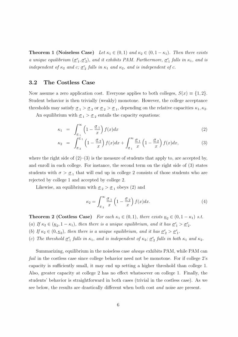
for minority students is illustrated in Figure 4.

This shift in student behavior disrupts the initial equilibrium, (σ01, σ

02). After the

introduction of the policy, applications to college 1 from minority students will increase,

and this leads to an increase in its admissions threshold. This effect is depicted in the

left panel of Figure 5 by a rightward shift in the H−11 function. Yet the increase in

σ 1 must be less than ∆, for otherwise enrollment would be strictly lower than it was

14

α1(x)

α 2(x)

0 1

1

Figure 4: Student Behavior with Race Based Admissions. With the introductionof a race based admissions policy, students in the minority group are more likely to get intocollege 1 than before. As a result, their acceptance relation shifts downward. Their newacceptance relation is indicated by the dotted line, while the old one is dashed. Note thatminority students start applying to college 1 at lower calibers than was previously the case.

initially. Hence the policy raises the admissions standard at college 1 for members of the

majority group, and lowers it for those in the minority. The size of the effect depends on

the fraction of minority students in the population: for ρ low, the shift in H−11 will be

small and the new threshold σ11 will only be marginally higher. This means that σ1

1−∆

will be close to σ01 −∆, and thus the minority group will receive the full benefit of the

policy. By contrast, for ρ high, the admissions standard will increase markedly, and the

new threshold for the minority group will not be that much lower. Moreover, that for

members of the majority group will be considerably higher.

To complete the analysis, we note that college 2 must similarly drop its admissions

threshold relative to before, as it is losing minority applicants to college 1. This is shown

in the right panel of Figure 5 by a downward shift in the H2 function. Yet since college

1 is simultaneously raising its applications threshold, thereby raising demand for places

at college 2 from students of the majority group, the overall effect on the applications

threshold of college 2 is unclear. We summarize our results in a proposition:

Theorem 7 (Race-Based Admissions) Consider a monotone equilibrium and let

college 1 implement a race-based admissions system parameterized by ∆. Then,

15

σ1

σ2

H1−1 H

2

H1’ −1

σ1

σ2

E1

E0

σ2

Figure 5: Equilibrium under Race Based Admissions The left panel shows theeffect of increased applications by minority students to college 1. The H−1

1 functions shiftsrightwards, intersecting H2 at a higher level of both σ 1 and σ 2. The right panel shows therightward shift of H2 that results from college 2 losing minority applicants. The equilibriumshifts from E0 to E1, with a clear increase in the applications threshold at college 1, but anambiguous effect on the applications threshold of college 2.

(i) The proportion of minority students at college 1 increases, and at college 2 falls;

(ii) The new threshold set by college 1 is higher, and is increasing in ρ;

(iii) The new threshold set by college 2 is the same as the old one.

These results provide some novel insights into the effects of these policies. The first

is that there is an implicit tradeoff between the level of diversity across colleges. Mak-

ing one college more diverse by attracting and admitting minority applicants through a

race-based admissions policy must in turn limit the fraction of minority applicants at

other schools. Moreover, these minority applicants may have less chance of being ad-

mitted at other schools as they are crowded out by strong majority applicants who were

discouraged from applying to the college with the race-based admissions policy. This

will be the case when the minority group is a small fraction of the population. So even

if achieving diversity across colleges is considered an appropriate aim, there is a need to

be sure that the schools that implement it are less diverse than their competitors.

The second insight relates to the composition of the student body at college 1. The

policy allows weaker students from the minority group admission into the school. But

it also restricts enrollment to stronger applicants from the majority group, and thus the

effects on the average caliber of students in the school are unclear. To the extent that

there are benefits to having a diverse student body, these benefits will be experienced

16

by all. The question then becomes whether the caliber of the learning experience is

dependent on the average caliber the student body, or is shaped by the weakest caliber

in the student population. If the former, there is no real tradeoff and the policy is good

for college 1; while if the latter, the effects of the policy are more tricky to pin down.

7 Different Signals of Caliber

7.1 Conditionally iid MLRP Signals

For simplicity, we have derived all the results under the assumption that the conditional

distribution of the signal for a student of caliber x is uniform on [0, x]. We now show

that all the results extend to a large class of signal distributions with the MLRP.

Let g(σ|x) be a continuous density function that satisfies the MLRP, with σ ∈ [σ, σ],

−∞ ≤ σ < σ ≤ ∞, x ∈ [x,∞), and x ≥ −∞. Let G(σ|x) be its cdf, which is assumed

to be twice differentiable in x. Since G is monotone in each variable, we can take the

inverse function with respect to each of them. We shall denote by ϕ the inverse of G

with respect to x, and by φ the corresponding one with respect to σ.

Inverting α1(x) = 1−G(σ 1|x) with respect to x and inserting the resulting expression

in α2(x) = 1−G(σ 2|x) yields the following acceptance relation:

α2 = ψ(σ 1, σ 2, α1) ≡ 1−G(σ 2|ϕ(1− α1, σ 1)). (23)

Inspired by the properties of the acceptance relation in the uniform case, we shall

impose the following assumptions on (23): (a) ψ is increasing in α1; (b) ψ(0, σ 1, σ 2) ≥ 0,

ψ(1, σ 1, σ 2) = 1, and 0 < ψ < 1 for all α1 ∈ (0, 1); (c) ψ is concave in α1 if σ 1 ≥ σ 2.

Under these conditions, we get an acceptance relation of the form depicted in Figure 6.

The following result provides a set of sufficient conditions on the family of signal

distributions that engender properties (a), (b), and (c).

Lemma 4 (Signal Distributions) ψ(σ 1, σ 2, α1) satisfies (a), (b), and (c), if:

(i) g(σ|x) satisfies MLRP;

(ii) For all interior σ and x, G(σ|x) > 0, limx→x G(σ|x) = 1 and limx→∞ G(σ|x) = 0;

(iii) −Gx(σ|x) is log-supermodular in (σ, x).

17

0 1

1

α1(x)

α 2(x)

Figure 6: Concave acceptance relation. The figure depicts an example of an acceptancerelation that satisfies conditions (a), (b), and (c), for which student behavior is monotone.

MLRP implies property (a), while (ii) yields the boundary conditions embedded in (b).

In turn, log-supermodularity of −Gx ensures the concavity property asserted in (c).

We will henceforth assume (i), (ii), and (iii). To be sure, this defines a large

class of signal distributions. One can easily show that it includes the location families

G(σ|x) = G(σ − x) (e.g., normal), the scale families G(σ|x) = G(σ/x) (e.g., uniform

and exponential), and also the oft-used in applications power family G(σ|x) = G(σ)x.

Careful inspection of the proofs of Theorems 1–3 reveal that they only make use

of properties (a) and (b) of the uniform distribution, and thus they readily extend to

the class of signal distributions defined in Lemma 4. Also, the construction of the

non-monotone equilibrium was independent of the signal distribution.

Notice that extension of Lemma 2 implies that of Lemma 3, since its proof does not

depend on the uniform distribution. Similarly, extension of Theorem 4 implies that of

Theorems 5 and 6, and Proposition 7, for their proofs do not depend on the uniform

distribution either. Thus, it only remains to extend Lemma 2 and Theorem 4. The

details can be found in the Appendix, but here is an overview of the main issues.

Regarding Lemma 2, the only problem that arises is that ξB need not be unique,

as it is defined by the solution of the acceptance relation (23) and the marginal benefit

function (8), both of which are concave functions. We show that the following condition

18

on the information structure is sufficient (but by no means necessary) for ξB to be

unique for c sufficiently small: If σ 1 ≥ σ 2 > σ, then

limx→x

(1−G(σ 1|x))Gx(σ 2|x)/Gx(σ 1|x) = 0. (24)

This is a relatively mild condition that is satisfied by most of the aforementioned exam-

ples (e.g., uniform, exponential, and product family).

Regarding Theorem 4, the analog to condition (15) in this case is:

1−G(σ 2|ϕ(1− α1, σ 1)) ≥1

uα1,

which is equivalent to

σ 2 ≤ φ(1− 1

uα1, ϕ(1− α1, σ 1)). (25)

This condition is now necessary but not sufficient for monotone behavior, since we also

need to ensure that ξB is unique. It is easy to show that the right side of (25) is increasing

in σ 1, strictly less than σ 1 for all c > 0, and converges to σ 1 as c vanishes.5

Assuming that ξB is unique, a monotone equilibrium is a pair of college thresholds

that satisfy equations (18) and (19) (with G(σ i|x) instead of σ i/x, i = 1, 2), as well as

condition (25). We show that if the signal distribution satisfies (24), then the existence

part of Theorem 4 holds. The uniqueness part holds if, in addition, it satisfies the

following condition: If σ 1 ≥ σ 2 > σ, then

limx→x

(1−G(σ 1|x))g(σ 2|x)/Gx(σ 1|x) = 0. (26)

Like (24), condition (26) is also satisfied by most of the examples mentioned above.6

In short, all the insights extend to a large class of information structures that satisfy

MLRP plus some regularity conditions. The role of the latter is simply to ensure that

student behavior will be monotone when college behavior is monotone.

5For example, in the location families with x = −∞, σ = −∞, and σ = ∞, the right side of (25)becomes σ 1−

(G−1(1− α1)−G−1(1− α1/u)

), while it is equal to

(1− log u

log α1

)σ 1 if g(σ|x) = 1

xe−σ/x,x = σ = 0, and σ = ∞. It is straightforward to check the aforementioned properties.

6Notice that (24) and (26) are satisfied if Gx(σ|x) 6= 0 and finite for all σ > σ, as in G(σ|x) = G(σ)x.

19

7.2 Perfectly Correlated Signals

So far we have assumed that if a student of caliber x applies to both colleges, they

observe independent signals drawn from g(σ|x). We now study the polar case in which

the signals observed by the colleges are perfectly (positively) correlated (i.e., both observe

the same realization). For simplicity, we present the main results assuming that signals

are uniformly distributed, and then sketch their straightforward generalization to the

class of signal distributions of Lemma 4. The key feature of this case is that if a student

is accepted at the more selective college, then he is also accepted at the less selective

one. This immediately implies that σ 1 > σ 2 in equilibrium, for otherwise nobody would

apply to college 2. That is, in any equilibrium college behavior must be monotone.

The expected utility of applying to just one college is α1(x) − c and α2(x)u − c,

respectively. Since σ 1 > σ 2, applying to both yields α1(x) + (α2(x) − α1(x))u − 2c.

Thus, the student’s optimal strategy is characterized by the following conditions:

α2u = α1

MB21 ≡ (α2 − α1)u = c

MB12 ≡ α1(1− u) = c.

Graphically, the following straight lines delimit the regions of the student’s application

strategy: α1 = c/(1 − u), α2 = α1 + c/u, α2 = α1/u, α1 = c, and α2 = c/u. Since the

acceptance relation (10) is also linear, student optimal behavior is always monotone. To

avoid the trivial case without multiple applications, we impose the condition that the

acceptance relation crosses above the point (α1, α2) = (c/(1−u), c/u(1−u)). This yields

σ 2 ≤(

1− c/u(1− u)

1− c/(1− u)

)σ 1. (27)

The thresholds ξ2, ξB, and ξ1 solve, respectively, α2(ξ2) = c/u, α2(ξB) = (1− σ 2

σ 1)+

σ 2

σ 1

c1−u

,

and α2(ξ1) = (1− σ 2

σ 1) +

σ 2

σ 1(α2(ξ1)− c/u). Easy algebra yields

ξ2 =σ 2

1− c/u

ξB =σ 1

1− c/(1− u)

ξ1 =u

c(σ 1 − σ 2).

20

0 1

1

α1(x)

α 2(x)

α

Figure 7: Student Behavior with perfectly correlated signals. With perfectlycorrelated signals, we get different acceptance regions from those in the independent case.

Notice that these thresholds satisfy all the properties stated in Lemma 2 except for one:

ξB does not depend σ 2. This dramatically simplifies the equilibrium analysis, for it

makes the determination of the acceptance threshold σ 1 independent of σ 2.

A monotone equilibrium is a pair of college thresholds that satisfies:

κ1 = E1(σ 1) (28)

κ2 = E2(σ 1, σ 2) (29)

0 ≤ σ 2 ≤(

1− c/u(1− u)

1− c/(1− u)

)σ 1, (30)

where

E1(σ 1) =

∫ ∞

ξB(σ 1)

(1− σ 1

x)f(x)dx

E2(σ 1, σ 2) =

∫ ξB(σ 1)

ξ2(σ 2)

(1− σ 2

x)f(x)dx +

∫ ξ1(σ 1,σ 2)

ξB(σ 1)

σ 1 − σ 2

xf(x)dx

Equations (28)–(29) define, implicitly, the functions σ 1 = H1(κ1) and σ 2 = H2(σ 1, κ2).

Theorem 8 (Perfectly Correlated Signals) Let κ1 ∈ (0, 1) and c < u(1− u).

21

(i) There is an interval (κ2(κ1), κ2(κ1)), with 0 < κ2(κ1) < κ2(κ1) < 1 − κ1, such

that, for all (κ1, κ2) ∈ (0, 1)× (κ2(κ1), κ2(κ1)), a unique equilibrium exists.

(ii) The comparative static properties with respect to κ1 and c are the same as in

Theorem 6, while an increase in κ2 reduces σe2 but has no effect on σe

1.

Notice that an increase in the capacity of college 2 has no effect on the acceptance thresh-

old of college 1. This is because the marginal benefit of adding college 1 to a portfolio

that already contains college 2 is independent of σ 2. Thus, ξB, which determines the

caliber above which students apply to college 1, does not depend on σ 2 either, thereby

insulating college 1’s applicant pool from the acceptance decisions of college 2 (i.e., the

H−11 function is a ‘vertical’ line). But this result only holds in the perfectly correlated

case and hence it is not robust. To see this, note that in the conditional independent

case MB12 = α1 − α1α2u; i.e., adding college 1 increases expected utility by α1 but it

decreases it by α1α2u, since acceptance by college 1 has an ‘opportunity cost’ of α2u.

In the perfectly correlated case, that opportunity cost is equal to u, as the probability

of being accepted at college 2 conditional on being accepted at college 1 is equal to one,

and thus it is independent of σ 2. But if correlation is less than perfect, this conditional

probability is less than one and depends on σ 2. Therefore, ξB will depend on σ 2 as

well. Graphically, this means that the slope of H−11 will be positive but less than infinity

unless the signals of a student observed by colleges are perfectly correlated.

Proposition 8 easily extends to the class of g(σ|x) of Lemma 4; just replace (27) by

σ 2 ≤ φ(1− c/u(1− u), ϕ(1− c/(1− u), σ 1)). (31)

The only additional insight that emerges in the general case is that, if ψ is strictly

concave, then there exists nonmonotone equilibria when condition (31) does not hold.

8 Conclusion

Assume, simply for the sake of argument, that Harvard is indeed the best college. Does

that mean that Harvard attracts the best students to apply to it? When the University

of Chicago increased the size of its college by a third, what should we expect were the

effects on its student caliber, or on other competing colleges? What are the effects of

the recent advances in technology that have reduced college application costs? How do

22

race-based admissions policies affect student body composition? These are some of the

issues this paper has been designed to answer, in an extremely stylized environment.

We have provided an intuitive graphical solution to the nontrivial student portfolio

choice problem, which clearly illustrates the lack of a natural single crossing property to

guarantee monotone behavior as a function of calibers. We have also explored assortive

matching in this context, showing that it arises provided the application cost is small

and the capacity of the lesser college is neither too large nor too small. We have shown

that there are also equilibria that are non-monotone; surprisingly, they exist even when

the better college sets a higher admission threshold than the lesser college. We have

provided equilibrium comparative static results with respect to college capacities and

application cost. Crucially, we have shown that noisy signals and student application

costs introduce an externality of the worse-ranked college upon the better one. This only

arises when both noise and cost are present, for it is driven by the subtle student portfolio

reallocation that ensues when a parameter changes. We have shown the robustness of our

main results by generalizing our model to a large class of signal distributions, explored

the case with correlated signals, and provided a foundation for our reduced-form model

of college behavior (see Appendix). Finally, we have presented an application to the

case of race-based admissions, and showcased some of the tradeoffs that arise there.

There are many natural avenues for future research. Obviously, as we have pro-

ceeded with just two colleges, this does not realistically capture the far richer world.

Also, college caliber is in the long-term endogenously determined by the caliber of stu-

dents attending. Finally, we have assumed that student preferences are homogeneous.

In Chade, Lewis, and Smith (2005) we allow for heterogenous preferences and investi-

gate — theoretically and empirically — the informational content of several equilibrium

statistics (e.g., acceptance rates, yields, etc.) that are commonly used as a basis for the

construction of college rankings.

23

A Appendix: Omitted Proofs

A.1 Proof of Theorem 1 (Noiseless Case)

(i) We can solve (1) sequentially as follows. For any κ1 ∈ (0, 1), there is a unique σe1

that solves the κ1 equation in (1), which is independent of σ 2 and is decreasing in κ1.

Inserting this solution in the κ2 equation, we find that the right side is decreasing in σ 2,

and its maximum value is equal to∫ σe

1

0f(x)dx = 1− κ1. Thus, if κ2 ∈ (0, 1− κ1), then

there is a unique σe2 that solves the second equality in (1). Hence, there is a unique pair

(σe1, σ

e2) that solves both equations in (1).

(ii) Notice that equations (1) do not depend on c. Next, differentiate (1). ¤

A.2 Proof of Theorem 2 (Costless Case)

(i) We can solve (2)–(3) sequentially as follows. For any κ1 ∈ (0, 1), there is a unique σe1

that solves equation (2), which is independent of σ 2 and is decreasing in κ1. Inserting

this solution in equation (3), we find that the right side is decreasing in σ 2, and its

maximum value — i.e., when σ 2 = 0 — is equal to∫ σe

1

0f(x)dx+

∫∞σe

1

σe1

xf(x)dx = 1−κ1.

Since the largest value σ 2 can assume in this case is σe1, it follows that the smallest

feasible value of the right side of (3) is equal to∫∞

σe1

σe1

x(1 − σe

1

x)f(x)dx. Call this value

κ2(κ1). Then, if κ2 ∈ (κ2(κ1), 1− κ1), there is a unique σe2 that solves (3). Hence, there

is a unique pair of college thresholds (σe1, σ

e2) that solves (2)–(3).

(ii) Let κ1 ∈ (0, 1). Proceeding as in (i) and inserting the unique solution σe1 of (2) in (4),

it follows that there is a unique solution σe2, with σe

1 < σe2, so long as κ2 ∈ (0, κ2(κ1)).

(iii) Notice that equations (2)–(3) (and (4)) do not depend on c. The rest follows by

straightforward differentiation of equations (2) and (3) (or (4)). ¤

A.3 Proof of Theorem 3 (Equilibrium Existence)

The enrollment functions have the following properties: (a) E1(0, σ 2) = 1; (b) E1(∞, σ 2) =

0 ∀σ 2; (c) E2(σ 1,∞) = 0 ∀σ 1; (d) E1 is decreasing in σ 1 and increasing in σ 2; (e) E2

is increasing in σ 1 and decreasing in σ 2. Now, (a), (b) and (d) imply that there exists

a unique σ 1 for any κ1 such that E1(σ 1, σ 2) = κ1. To get a similar existence statement

for E2(σ 1, σ 2) we must bound σ 1 away from 0 (otherwise college 2 will be unable to fill

its capacity). Let σL1(κ2) be defined by E2(σ

L1, 0) = κ2. Then by (e) for σ 1 ≥ σL

1(κ2)

24

there exists a unique σ 2 ≥ 0 such that E2(σ 1, σ 2) = κ2. But since we restrict college 1

to a threshold of at least σL1(κ2), it is clear that it cannot have ‘large capacity.’ More

precisely, let κH1 (κ2) = E1(σ

L1(κ2), 0). Then for any κ1 ≤ κH

1 (κ2), there will be a unique

solution for σ 1, with σ 1 ≥ σL1(κ2) for all σ 2. We may show that this restriction on κ1

is equivalent to requiring κ2 to be less than κ2(κ1) for κ2(κ1) = E2(H1(0, κ1), 0).

Note that the colleges cannot set thresholds above a certain level. Certainly, college

1 cannot set a threshold higher than σH1 , where σH

1 (which determines α1(x)) solves

∫ ∞

0

α1(x)f(x)dx = κ1,

for the set of calibers applying to college 1 is a subset of [0,∞). Similarly, we define σH2 .

So fix κ1 and κ2 as in the statement, and define the space S = [σL1, σ

H1 ] × [0, σH

2 ],

which is compact, convex and nonempty. Define a vector-valued function T : S → S by

T (σ 1, σ 2) = (σ 1, σ 2), where σ 1 satisfies E1(σ 1, σ 2) = κ1 and σ 2 satisfies E2(σ 1, σ 2) =

κ2. T is well-defined on S, as shown by the earlier analysis. Further, T is continuous, as

the demand functions are continuous in both arguments. The latter follows since the cal-

iber distribution is atomless, and both the application sets and acceptance probabilities

are smooth functions of the thresholds. Thus we may apply Brouwer’s fixed point theo-

rem to deduce that T has a fixed point — which immediately satisfies κ1 = E1(σ 1, σ 2)

and κ2 = E2(σ 1, σ 2). ¤

A.4 Proof of Lemma 1 (Thresholds for Monotone Strategies)

The threshold ξ2 solves α2(ξ2) = c/u, which immediately yields (12).

Threshold ξB is derived in two steps. We first find the value of α1 at which the

acceptance relation α2 = ψ(σ 1, σ 2, α1) intersects α2 = (1− c/α1)/u. Call this value α1,

which is the unique solution in (0, 1) (i.e., the smallest solution) to the equation

α21 −

(1 +

(1− u)

u

σ 1

σ 2

)α1 +

c

u

σ 1

σ 2

= 0.

Given α1, we then find ξB as α1 = 1 − G(σ 1|ξB), which yields ξB = σ 1/(1 − α1).

Expression (13) follows by simple algebraic manipulation.

Finally, ξ1 is obtained as follows. We first find the value of α1 at which the acceptance

relation α2 = ψ(σ 1, σ 2, α1) intersects α2 = c/(1− α1)u. Call this value α1, which is the

25

unique solution in (0, 1) (i.e., the largest solution) to the equation

(1− α1)

(1− σ 2

σ 1

(1− α1)

)− c

u= 0.

Given α1, we then find ξ1 as α1 = 1−G(σ 1|ξ1), which yields ξ1 = σ 1/(1−α1). Expression

(14) follows by simple algebraic manipulation.

A.5 Proof of Lemma 2 (Monotone Student Behavior)

Since the proof amounts to straightforward and tedious differentiation and limit-taking

of the closed form expressions (12)–(14), we shall prove parts (ii) and (iii) in a way that

generalizes beyond the uniform distribution. Firstly, (i) is obvious from (12)

(ii) Notice that α1 satisfies

α1 =c

1− uψ(σ 1, σ 2, α1). (32)

Denote the right side of (32) by z(α1, c, u, σ 1, σ 2). It is easy to show that

0 < z(0, c, u, σ 1, σ 2) < z(1, c, u, σ 1, σ 2) < 1,

z(α1, c, u, σ 1, σ 2) is strictly increasing in α1 and, under the uniform distribution, it

is also strictly convex in α1. Thus, there is a unique α1 that satisfies (32). Moreover,

z(α1, c, u, σ 1, σ 2) decreases σ 2, increases in c and σ 1, and converges to zero as c vanishes.

Hence, α1 exhibits this behavior as well. Since ξB = σ 1/(1− α1), the properties stated

in part (ii) now follow easily.

(iii) Notice that α1 satisfies

α1 = 1− c

uψ(σ 1, σ 2, α1). (33)

Denote the right side of (33) by r(α1, c, u, σ 1, σ 2). It is easy to show that (recall (15))

α1 < r(α1, c, u, σ 1, σ 2) < r(1, c, u, σ 1, σ 2) < 1,

r(α1, c, u, σ 1, σ 2) is strictly increasing in α1 and, since ψ is concave in α1 under the

uniform distribution, r(α1, c, u, σ 1, σ 2) is also strictly concave in α1. Thus, there is

26

a unique α1 ∈ (α1, 1) that satisfies (33). Moreover, r(α1, c, u, σ 1, σ 2) decreases in c

and σ 2, increases in σ 1, and converges to one as c vanishes. Hence, α1 exhibits these

properties as well. Since ξ1 = σ 1/(1− α1), part (iii) is now straightforward. ¤

A.6 Proof of Theorem 4 (Monotone Equilibrium)

Let κ1 ∈ (0, 1) be given, and let η ≡(

1−α1/u1−α1

). We shall denote by (σ1, σ2) the unique

solution to κ1 = E1(σ 1, σ 2, c) and σ 2 = ησ 1. Obviously, (σ1, σ2) depend on κ1 and c.

Existence. To prove existence, we proceed in four steps. First, we show that there is

an interval of κ2 such that the value of σ 1 at which H2(σ 1, κ2, c) = 0 is less than the

value of σ 1 at which σ 1 = H1(0, κ2, c). Second, we show that there exists an interval

of κ2 such that, at σ1, H2(σ1, κ2, c) < σ2. Third, we prove that if c is sufficiently small,

then the intersection of the aforementioned intervals is nonempty. Fourth, we use the

continuity of the functions H1 and H2 to complete the existence proof.

Step 1: There is an interval of κ2 such that H−12 (0, κ2) < H1(0, κ1).

To see this, note first that σ 1 = H1(0, κ1, c) is the unique solution to κ1 = E1(σ 1, 0, c).

Also, it is easy to show that, at σ 2 = 0, ξ2 = 0, ξB = σ 1/(1−c/(1−u)), and ξ1 = σ 1u/c.

Thus, κ2 = E(σ 1, 0, c) is given by

κ2 =

∫ σ 1(1−u)

1−u−c

0

f(x)dx +

∫ σ 1u

c

σ 1(1−u)

1−u−c

σ 1

xf(x)dx. (34)

Since E2(0, 0, c) = 0 and ∂E2/∂σ 1 > 0, it follows that if κ2 ∈ (0, E2(H1(0, κ1, c), 0, c)),

then the unique solution to (34) satisfies H−12 (0, κ2, c) < H1(0, κ1, c).

Step 2: There is an interval of κ2 such that H2(σ1, κ2, c) < σ2 = ησ1.

Since ∂E2/∂σ 2 < 0, it follows that if κ2 ∈ (E2(σ1, σ2, c), E2(σ1, 0, c)), then the unique σ 2

that solves κ2 = E2(σ1, σ 2, c) belongs to the interval (0, σ2), and thus H2(σ1, κ2, c) < σ2.

Step 3: For c small, the intersection of the two intervals of κ2 is an interval.

We will show that E2(σ1, σ2, c) < E2(H1(0, κ1, c), 0, c)) for c > 0 sufficiently small. Let

us write σ1(κ1, c) and σ2(κ1, c) to emphasize their (continuous) dependence on κ1 and

c. Since α1 = (1−√1− 4c)/2, limc→0 α1 = 0 and thus σ2(κ1, 0) = σ1(κ1, 0). Notice also

that κ1 = E1(σ1(κ1, 0), σ1(κ1, 0), 0) implies that σ1(κ1, 0) > 0, as E1(0, σ 2, c) = 1 > κ1.

Moreover, H1(0, κ1, 0) = σ1(κ1, 0), for ξB is equal to σ 1 at c = 0 (Lemma 2 (ii)) and

27

thus is independent of σ 2.7 Using these results and Lemma 2, it follows that

limc→0

E2(σ1(κ1, c), σ2(κ1, c), c) =

∫ ∞

σ1(κ1,0)

σ1(κ1, 0)

x(1− σ1(κ1, 0)

x)f(x)dx

limc→0

E2(H1(0, κ1, 0), 0, c) =

∫ σ1(κ1,0)

0

f(x)dx +

∫ ∞

σ1(κ1,0)

σ1(κ1, 0)

xf(x)dx.

Thus, E2(σ1(κ1, 0), σ2(κ1, 0), 0) < E2(σ1(κ1, 0), 0, 0). By continuity, E2(σ1, σ2, c) <

E2(H1(0, κ1, c), 0, c)) for c > 0 sufficiently small.

Step 4: Given κ1, an equilibrium exists for an interval of c and an interval of κ2.

Define κ2(κ1) ≡ E2(σ1, σ2, c) and κ2(κ1) ≡ E2(H1(0, κ1, c), 0, c). Thus far we have shown

that if c ∈ (0, c0(κ1)) and κ2 ∈ (κ2(κ1), κ2(κ1)), then H−12 (0, κ2) < H1(0, κ1) (Step 1)

and H2(σ1, κ2, c) < H−1(σ1, κ1, c) (Step 2 plus the definition of σ1). In words, within the

set of (σ 1, σ 2) such that 0 ≤ σ 2 ≤ ησ 1, the function σ 2 = H−11 (σ 1, κ1, c) lies ‘below’

the function σ 2 = H2(σ 1, κ2, c) for low values of σ 1 (Step 1) and ‘above’ when σ 1 = σ1.

Since H1 and H2 (as well as their inverses) are continuous, it follows that a monotone

equilibrium (σe1, σ

e2) exists.

Uniqueness. We now show that if κ2 ∈ (κ2(κ1), κ2(κ1)) and c is small, then the slope

of σ 2 = H2(σ 1, κ2, c) is smaller than that of σ 2 = H−11 (σ 1, κ1, c), thereby implying that

the equilibrium is unique. Formally, we need to show that ∂H1/∂σ 2× ∂H2/∂σ 1 < 1, or

∂E1/∂σ 1 × ∂E2/∂σ 2 − ∂E1/∂σ 2 × ∂E2/∂σ 1 > 0. (35)

Differentiation of expressions (12)–(14) and (16)–(17) yields after tedious algebra

limc→0

∂E1/∂σ 2 = 0

limc→0

∂E2/∂σ 1 =

∫ ∞

σ 1

(1− σ 2

x)f(x)

xdx

limc→0

∂E1/∂σ 1 = −∫ ∞

σ 1

f(x)

xdx

limc→0

∂E2/∂σ 2 = −∫ σ 1

σ 2

f(x)

xdx−

∫ ∞

σ 1

σ 1

x

f(x)

xdx.

Hence, (35) holds at c = 0. By continuity, the result also holds for c ∈ (0, c1(κ1)).

7Graphically, σ 2 = H−11 (σ 1, κ1, c) becomes a ‘vertical line’ as c goes to zero; recall the costless case.

28

Let c(κ1) = min{c0(κ1), c1(κ1)}. Given κ1 ∈ (0, 1), we have thus proved that there

is a unique monotone equilibrium (σe1, σ

e2) if κ2 ∈ (κ2(κ1), κ2(κ1)) and c ∈ (0, c(κ1)). ¤

A.7 Proof of Theorem 5 (Types under PAM)

Let f1(x) and f2(x) be the densities of calibers accepted at colleges 1 and 2, respectively,

where we have omitted (σe1, σ

e2) to simplify the notation. Formally,

f1(x) =α1(x)f(x)∫∞

ξBα1(t)f(t)dt

I[ξB ,∞)(x) (36)

f2(x) =I[ξ2,ξB ](x)α2(x)f(x) + (1− I[ξ2,ξB ](x))α2(x)(1− α1(x))f(x)∫ ξB

ξ2α2(s)f(s)ds +

∫ ξ1ξB

α2(s)(1− α1(s))f(s)dsI[ξ2,ξ1](x), (37)

where IA is the indicator function of the set A.

We shall show that, if xL, xH ∈ [0,∞), with xH > xL, then f1(xH)f2(xL) ≥f2(xH)f1(xL); i.e., fi(x) is log-supermodular in (−i, x), or it satisfies MLRP. Since MLRP

of the densities implies that the cdfs are ordered by FSD, the theorem follows.

Using (36) and (37), f1(xH)f2(xL) ≥ f2(xH)f1(xL) is equivalent to

α1HI[ξB ,∞)(xH)(I[ξ2,ξB ](xL)α2L + (1− I[ξ2,ξB ](xL))α2L(1− α1L)

)I[ξ2,ξ1](xL) ≥

α1LI[ξB ,∞)(xL)(I[ξ2,ξB ](xH)α2H + (1− I[ξ2,ξB ](xH))α2H(1− α1H)

)I[ξ2,ξ1](xH),

(38)

where αij = αi(xj), i = 1, 2, j = L,H. It is easy to show that the only nontrivial case

to consider is when xL, xH ∈ [ξB, ξ1] (in all the other cases, either both sides are zero,

or only the right side is). If xL, xH ∈ [ξB, ξ1], then (38) becomes α1Hα2L(1 − α1L) ≥α1Lα2H(1− α1H), or

(1−G(σ 1 | xH))(1−G(σ 2 | xL))G(σ 1 | xL) ≥(1−G(σ 1 | xL))(1−G(σ 2 | xH))G(σ 1 | xH).

(39)

Since g(σ | x) satisfies MLRP, it follows that (i) G(σ | x) is decreasing in x, and hence

G(σ 1 | xL) ≥ G(σ 1 | xH); (ii) 1−G(σ | x) is log-supermodular in (x, σ), and therefore

(1 − G(σ 1 | xH))(1 − G(σ 2 | xL)) ≥ (1 − G(σ 1 | xL))(1 − G(σ 2 | xH)), for σ 1 > σ 2

in a monotone equilibrium. Thus, (39) is satisfied, thereby proving that fi(x) is log-

supermodular, which in turn implies that F1 dominates F2 is the sense of FSD. ¤

29

A.8 Proof of Theorem 6 (Comparative Statics)

(i) In equilibrium, κ1 = E1(σe1, σ

e2, c) and κ2 = E2(σ

e1, σ

e2, c). Differentiating this system

with respect to κ1, yields

∂σe1

∂κ1

=

∂E2

∂σe2

∆< 0

∂σe2

∂κ1

=− ∂E2

∂σe1

∆< 0,

where ∆ = ∂E1/∂σe1 × ∂E2/∂σe

2 − ∂E2/∂σe1 × ∂E1/∂σe

2 > 0 (see Theorem 4).

(ii) Differentiating κ1 = E1(σe1, σ

e2, c) and κ2 = E2(σ

e1, σ

e2, c) with respect to κ2 yields

∂σe1

∂κ2

=− ∂E1

∂σe2

∆< 0

∂σe2

∂κ2

=

∂E1

∂σe1

∆< 0,

where ∆ = ∂E1/∂σe1 × ∂E2/∂σe

2 > 0.

(iii) Differentiating κ1 = E1(σe1, σ

e2, c) and κ2 = E2(σ

e1, σ

e2, c) with respect to c yields

∂σe1

∂c=−∂E1

∂c∂E2

∂σe2

+ ∂E2

∂c∂E1

∂σe2

∆< 0

∂σe2

∂c=− ∂E1

∂σe1

∂E2

∂c+ ∂E2

∂σe1

∂E1

∂c

∆≷ 0

To see this, notice that the numerator of ∂σe1/∂c is negative, since it is given by

(1−σ 1

ξB

)f(ξB)

(−A(1− σ 2

ξ2

)f(ξ2) + Bσ 1

ξ1

(1− σ 2

ξ1

)f(ξ1)−∫ ξ1

ξB

f(x)

xdx− σ 1

∫ ∞

ξB

f(x)

x2dx

),

where (using Lemma 2)

A =∂ξB

∂c

∂ξ2

∂σ 2

− ∂ξB

∂σ 2

∂ξ2

∂c> 0

B =∂ξB

∂c

∂ξ1

∂σ 2

− ∂ξB

∂σ 2

∂ξ1

∂c< 0.

In turn, the numerator of ∂σe2/∂c is given by

C(1− σ 1

ξB

)f(ξB)σ 1

ξ1

(1− σ 2

ξ1

)f(ξ1)−D(1− σ 1

ξB

)f(ξB) + E

∫ ∞

ξB

f(x)

xdx,

30

where (using Lemma 2)

C =∂ξB

∂σ 1

∂ξ1

∂c− ∂ξB

∂c

∂ξ1

∂σ 1

< 0

D = (1− σ 2

ξ2

)f(ξ2)∂ξ2

∂c

∂ξB

∂σ 1

+

(∫ ξ1

ξB

(1− σ 2

x)f(x)

xdx− (1− σ 2

ξB

)

∫ ∞

ξB

f(x)

xdx

)∂ξB

∂c≷ 0

E = −(1− σ 2

ξ2

)f(ξ2)∂ξ2

∂c+

σ 1

ξ1

(1− σ 2

ξ1

)f(ξ1)∂ξ1

∂c< 0,

thereby revealing that the sign of ∂σe2/∂c is ambiguous. ¤

A.9 Proof of Theorem 7 (Race Based Admissions)

Let Emi (σ 1 −∆, σ 2) be the minority students enrollment at college i, and EM

i (σ 1, σ 2)

be the majority students enrollment at college i, i = 1, 2. In (a monotone) equilibrium

κ1 = ρEm1 (σe

1 −∆, σe2) + (1− ρ)EM

1 (σe1, σ

e2) (40)

κ2 = ρEm2 (σe

1 −∆, σe2) + (1− ρ)EM

2 (σe1, σ

e2). (41)

To analyze the effects of introducing ∆, we will analyze the equilibrium comparative

static with respect to ∆ evaluated at ∆ = 0. Notice that, at ∆ = 0, Emi = EM

i , i = 1, 2,

and the same is true with their derivatives.

(i) Note that, with the introduction of ∆, ξB and ξ1 fall for minority students. Since

(ξB,∞) and (ξ2, ξ1) are, respectively, the sets of minority students calibers applying to

college 1 and to college 2, it follows that more of them now apply to college 1 and fewer

to college 2. Moreover, each minority student from the original equilibrium now has a

higher chance of getting into college 1, and the same chance of getting into school 2 as

their majority counterparts. Combining these effects (i.e. the application sets and the

acceptance probabilities), the result follows.

(ii) Differentiating (40)–(41) with respect to ∆, and evaluating the resulting expressions

at ∆ = 0 yields ∂σe1/∂∆ = ρ, which is positive, less than one, and increasing in ρ.

(iii) Proceeding as in (ii), we obtain that, evaluated at ∆ = 0, ∂σe2/∂∆ = 0. ¤

31

A.10 Proof of Lemma 4 (MLRP Families)

(a) ψ is increasing in α1, for

∂ψ

∂α1

= Gx(σ 2|φ(1− α1, σ 1))/Gx(σ 2|φ(1− α1, σ 1)),

and MLRP implies that Gx < 0.

(b) 0 < ψ < 1 for all α1 ∈ (0, 1) follows from G(σ|x) > 0 for every interior σ, x <

φ(1 − α1, σ 1) < ∞, and σ 1 ≥ σ 2. To show that ψ(0, σ 1, σ 2) ≥ 0, notice that ψ is

positive, single-valued, and continuous for all α1 ∈ (0, 1). Finally, limx→∞ G(σ|x) = 0

implies that limα1→1 φ(1−α1, σ 1) = ∞, and thus ψ(1, σ 1, σ 2) = limx→∞ 1−G(σ 2|x) = 1.

(c) ψ is concave in α1, for

∂2ψ

∂α21

=Gx(σ 2|ϕ(1− α1, σ 1))

Gx(σ 1|ϕ(1− α1, σ 1))2

(Gxx(σ 1|ϕ(1− α1, σ 1))

Gx(σ 1|ϕ(1− α1, σ 1))− Gxx(σ 2|ϕ(1− α1, σ 1))

Gx(σ 2|ϕ(1− α1, σ 1))

),

and this derivative is nonpositive if the expression in parenthesis is nonnegative. A

sufficient condition for this to hold is that Gxx(σ|x)/Gx(σ|x) be increasing in σ or,

equivalently, that −Gx(σ|x) be log-supermodular. ¤

A.11 Proof of Theorem 8 (Correlated Signals)

(i) It is easy to show that ∂E1

∂σ 1< 0, ∂E2

∂σ 2< 0, and ∂E2

∂σ 1> 0. Fix any κ1 ∈ (0, 1), and let

λ ≡(

1−c/u(1−u)1−c/(1−u)

). Then there exists a unique σe

1 that solves (28), which is decreasing

in κ1 and independent of σ 2. Inserting this solution in equation (29), we find that the

right side is decreasing in σ 2, and its maximum value — i.e., when σ 2 = 0 — is equal

to E2(σe1, 0). Call this value κ2(κ1). Since the largest value σ 2 can assume in this case

is λσe1, it follows that the smallest feasible value of the right side of (29) is equal to

E2(σe1, λσe

1). Call this value κ2(κ1). Then, if κ2 ∈ (κ2(κ1), κ2(κ1)), there is a unique σe2

that solves (29). Hence, there is a unique pair of college thresholds (σe1, σ

e2) that solves

(28)–(30). It is straightforward to check that 0 < κ2(κ1) < κ2(κ1) < 1− κ1.

(ii) In equilibrium, κ1 = E1(σe1, c) and κ2 = E2(σ

e1, σ

e2, c). Differentiating this system

32

with respect to κi, i = 1, 2, yields

∂σe1

∂κ1

=

∂E2

∂σe2

∆< 0

∂σe2

∂κ1

=− ∂E2

∂σe1

∆< 0

∂σe1

∂κ2

= 0∂σe

2

∂κ2

=

∂E1

∂σe1

∆< 0,

where ∆ = ∂E1/∂σe1 × ∂E2/∂σe

2 > 0. Differentiation with respect to c yields

∂σe1

∂c=

∂E1

∂c∂E2

∂σ 2

∆< 0

∂σe2

∂c=− ∂E1

∂σe1

∂E2

∂c+ ∂E2

∂σe1

∂E1

∂c

∆≷ 0

since ∂E1/∂c < 0 but the sign of ∂E2/∂c is ambiguous. ¤

B Appendix: General Signal Structure and PAM

Let xu(σ i) = max{x ∈ [x,∞)|G(σ i|x) = 1}, i = 1, 2 (e.g., in the uniform, xu(σ i) = σ i).

Consider the extension of Lemma 2. Part (i) follows easily, since α2(ξ2) = c/u

implies that ξ2 = φ(1 − c/u, σ 2), which is increasing in c and in σ 2. Moreover, since

ξ2 ∈ [xu(σ 2),∞) and is continuous in c, limc→0 ξ2 = xu(σ 2). The proof of part (iii) is

exactly the same as before, except that now ξ1 = φ(1− α, σ 1). Regarding part (ii), the

problem in the general case is that, although there is a solution α1 to equation (32) with

the properties stated in the proof, it need not be unique. Hence, ξB = φ(1− α1, σ 1) need

not be unique either. It is clear from (32) that a sufficient condition for uniqueness is

that the slope of z(α1, c, u, σ 1, σ 2) be less than one at any solution α to (32). Formally,

∂z

∂α1

=uα1

∂Ψ∂α1

1− uΨ< 1,

where we have omitted the arguments of the functions to simplify the notation. Now, as

c vanishes, the denominator converges to a positive number, and the numerator vanishes

if α1∂Ψ/∂α1 goes to zero. But this is equivalent to

limc→0

(1−G(σ 1|ξB))Gx(σ 2|ξB)

Gx(σ 1|ξB)= 0. (42)

Since ξB ∈ [xu(σ 1),∞) and is continuous in c, it follows that limc→0 ξB = xu(σ 1) ≥ x.

33

Thus, a sufficient condition for (42) is that condition (26) holds. Hence, ξB is unique for

an interval of c > 0 sufficiently small. The rest of the proof of (ii) is the same as before.

Let us turn now to Theorem 4. Assume for a moment that ξB is unique.

As regards to existence, the proof goes through with the following minor modifica-

tions. In Step 1, replace σ 2 = 0 by σ 2 = σ, σ 1/x by G(σ 1|x), and use ξ2 = x, ξB =

φ(1− c/u, σ 1), and ξ1 = φ(c/u, σ 1). In Step 2, replace ησ 1 by φ(1− 1uα1, ϕ(1−α1, σ 1)),

and 0 by σ. In Step 3, replace σ i = 0 (whenever it appear) by σ i = σ, i = 1, 2; replace

ξB = σ 1 at c = 0 by ξB = xu(σ 1) at c = 0, andσ1(κ1,0)

xby G(σ1(κ1, 0)|x). Finally, in

Step 4, replace 0 by σ inside E2, H1, and H−12 , and ησ 1 by φ(1− 1

uα1, ϕ(1− α1, σ 1)).

Regarding uniqueness, differentiation of ξ1 = φ(1 − α, σ 1) and ξB = φ(1 − α1, σ 1)

reveals, after some manipulation, that ∂ξ1/∂σ 1×∂ξB/∂σ 2 = ∂ξ1/∂σ 2×∂ξB/∂σ 1. Using

this result, one can show after much algebra that the slope condition (35) becomes:

−(1−G(σ 1|ξB))f(ξB) ∂ξB

∂σ 2

∫ ξ1ξB

g(σ 1|x)(1−G(σ 2|x))f(x)dx

− ∂E2

∂σ 2

∫∞ξB

g(σ 1|x)f(x)dx + D< 1, (43)

where D is a sum of positive terms. Since − ∂E2

∂σ 2>

∫ ξ1ξB

G(σ 1|x)g(σ 2|x)f(x)dx, D > 0,

and∫ ξ1

ξBg(σ 1|x)(1 − G(σ 2|x))f(x)dx >

∫∞ξB

g(σ 1|x)f(x)dx, it follows that a sufficient

condition for (43) to hold is that

−(1−G(σ 1|ξB))f(ξB) ∂ξB

∂σ 2∫ ξ1ξB

G(σ 1|x)g(σ 2|x)f(x)dx< 1. (44)

If condition (26) holds, then the numerator of (44) converges to zero as c vanishes, for∂ξB

∂σ 2= (c u g(σ 2|ξB))/(Gx(σ 1|ξB)((1 − uΨ)2 − cu∂Ψ/∂α1)). The denominator of (44)

converges to∫∞

xu(σ 1)G(σ 1|x)g(σ 2|x)f(x)dx > 0. Hence, (44) holds at c = 0 and, by

continuity, for small c > 0. Thus, (43) holds for small c > 0, and uniqueness follows.

So far we have assumed that ξB is unique. But this is true for small c > 0 if

condition (42) holds, since the equilibrium thresholds are continuous in c.

C Appendix: The College Objective Function

We now show that the reduced-form model of college behavior used in the paper can be

rationalized as a game between the two colleges, in which their objective is to maximize

34

the total expected caliber of the student body, subject to a capacity constraint.

Let B = {x | S(x) = {2}}, C = {x | S(x) = {1, 2}}, D = {x | S(x) = {1}}, and let

A1 = C ∪ D and A2 = B ∪ C be the number of students who apply to college 1 and

college 2. To avoid trivialities, let∫

Aif(x)dx > κi, i = 1, 2; i.e., each college receives

more applicants than the number of slots available. For simplicity, we assume that x ≥ 0.

Let gi(σ) =∫

Aig(σ|x)f(x)dx be the density of signals given the set of applicants Ai,

i = 1, 2, where g(σ|x) is any density with the MLRP. Also, let fi(x|σ) = g(σ|x)f(x)gi(σ)

be the

conditional density of x given σ and Ai, i = 1, 2.

With some abuse of notation, let ai(σ) be the probability that a student who has

applied to i and whose signal was σ accepts college i, and let γi(σ) be the expected value

of the student’s caliber given that he applies to i, his signal is γ, and he accepts college

i.

A strategy for college i, i = 1, 2, is a (measurable) indicator function χi : [σ, σ] →{0, 1}; i.e., a college chooses the set of signal realizations that it will accept. Then college

i’s optimization problem is given by

maxχi(σ)

∫ σ

σ

χi(σ)ai(σ)γi(σ)gi(σ)dσ (45)

subject to ∫ σ

σ

χi(σ)ai(σ)gi(σ)dσ ≤ κi. (46)

Note that constraint (46) must be binding at the optimum, for all students admitted

add to total caliber. Let λi, i = 1, 2, be the multiplier associated with (46). Forming

the Lagrangian and optimizing pointwise reveals that the optimal strategy is

χi(σ) =

1 if γi(σ) ≥ λi

0 if γi(σ) < λi,(47)

where λi is the ‘shadow price’ of each slot available at college i.

If we can show that γi(σ) increases in σ for each college i, then the optimal χi(σ) will

be represented by a threshold σ i such that each college accepts students whose signals

are above σ i, i = 1, 2. And since (46) holds with ecaliber for each college, this will

immediately justify the use of the reduced-form model.

Consider college 1. Since it is the best college, obviously a1(σ) = 1 for all σ. Thus,

35

γ1(σ) =∫

A1xf1(x|σ)dx, for being accepted by a student is uninformative. The MLRP

of g(σ|x) implies the MLRP of f1(x|σ), and therefore γ1(σ) is increasing in σ and college

1’s optimal strategy is summarized by a threshold σ 1. Notice that, for given applicant

pools, the determination of σ 1 is independent of the strategy used by college 2.

Consider college 2. Now a2(σ) is given by

a2(σ) =

∫

B

f2(x|σ)dx +

∫

C

G(σ 1|x)f2(x|σ)dx. (48)

That is, a given signal σ could come from a student who only applied to college 2, or

from one who applied to both colleges and was rejected from college 1. Therefore,

γ2(σ) =

∫B

xf2(x|σ)dx +∫

CxG(σ 1|x)f2(x|σ)dx

a2(σ). (49)

It is easy to show that γ2(σ) <∫

A2xf2(x|σ)dx. This is because being accepted by a

student reduces college 2’s estimate of his caliber, as there is a positive probability that

the student was rejected by college 1; i.e., college 2 suffers an acceptance curse effect.

Notice that equation (49) can be written as γ2(σ) =∫

A2xh2(x|σ)dx, where

h2(x|σ) =(IB(x) + ICG(σ 1|x))f2(x|σ)∫

A2(IB(x) + ICG(σ 1|x))f2(x|σ)dx

, (50)

where IB(x) (IC(x)) is the indicator function of the set B (C). It is immediate that the

‘density’ h2(x|σ) has the MLRP if f2(x|σ) does, which in turn follows from the MLRP of

g(σ|x). Therefore, γ2(σ) increases in σ, and the optimal χ2(σ), given σ 1, is summarized

by a threshold σ 2 such that students are accepted if only if their signal σ is above σ 2.

References

Albrecht, J., P. Gautier, and S. Vroman (2002): “Equilibrium Directed Search

with Multiple Applications,” Georgetown mimeo.

Anderson, A., and L. Smith (2005): “Assortative Matching and Reputation,” Uni-

versity of Michigan mimeo.

36

Becker, G. (1973): “A Theory of Marriage: Part I,” Journal of Political Economy,

81, 813–846.

Burdett, K., and K. Judd (1983): “Equilibrium Price Dispersion,” Econometrica,

51(4), 955–69.

Burdett, K., S. Shi, and R. Wright (2001): “Pricing and Matching with Frictions,”

Journal of Political Economy, 109(5), 1060–1085.

Chade, H. (2006): “Matching with Noise and the Acceptance Curse,” forthcoming,

Journal of Economic Theory.

Chade, H., G. Lewis, and L. Smith (2005): “What’s in a Ranking?,” work in

progress, University of Michigan.

Chade, H., and L. Smith (2006): “Simultaneous Search,” forthcoming in Economet-

rica.

Gale, D., and L. Shapley (1962): “College Admissions and Stability of Marriage,”

American Mathematical Monthly, 69(1), 9–15.

Kircher, P. (2006): “Simultaneous Directed Search with Recall,” mimeo, University

of Bonn.

Kircher, P., and M. Galenianos (2006): “Directed Search with Multiple Job Ap-

plications,” mimeo, University of Bonn.

Nagypal, E. (2004): “Applications with Incomplete Information,” mimeo, Northwest-

ern University.

Roth, A., and M. Sotomayor (1990): “The College Admissions Problem Revisited,”

Econometrica, 57(3), 559–570.

Shimer, R., and L. Smith (2000): “Assortative Matching and Search,” Econometrica,

68(2), 343–369.

Smith, L. (1997): “The Marriage Model with Search Frictions,” MIT working Paper.

37