The climate of Mars from assimilations of

Mars Climate Sounder data

DPhil 1st Year Report

Tao Ruan

Atmospheric, Oceanic and Planetary Physics

(AOPP)

Department of Physics

Lincoln College

University of Oxford

Supervisors

Professor Peter Read (University of Oxford)

Dr. Stephen Lewis (The Open University)

Word Count: 14379

Acknowledgements

I would like to express my gratitude to both of my supervisors Prof. Peter Read and

Dr. Stephen Lewis for their priceless advice and idea, the codes they share with me,

and especially for their understanding of my personal circumstance.

Besides I also want to thank M. D. Smith, NASA-Goddard Space Flight Center for

providing the MGS/TES observations and Dr. Luca Montabone for preparing the data

for data assimilation tests and the assimilation results analyzed in the Chapter 3.

Abstract

The works carried out during the first year of my DPhil project are presented in this

report. The objective of this project is to make use of a unique and advanced data

assimilation system that enables the combining of observational data with predictions

from a global numerical model of the Martian atmospheric circulation. In this report,

an introduction to the planet Mars and a brief description of observations used in this

project will be included, as well as an overview of modeling works conducted in

Oxford and by other groups, mainly on dust-related topics. Following the introduction,

we present a brief description of the Martian General Circulation Model (MGCM)

employed in this project. A new data assimilation approach will be developed based

on the MGCM described in this report. A study of semi-annual oscillations on Mars

from diagnostics of the assimilation results of Montabone et al. [2005] will be

presented as well. A clear signature of semi-annual oscillations is observed in the

assimilation results, and detailed analysis by Singular Spectrum Analysis (SSA) also

gives us a better understanding of this semi-annual cycle. Meanwhile, the first attempt

to develop an advanced data assimilation technique that includes a full assimilation of

3-D dust measurements into a moel that represents the full dust transport cycle is also

an important aim of this report. The progress achieved so far on the latest 2-D dust

data assimilation scheme with dust transport is encouraging for the development of

future 3-D dust data assimilation scheme with dust transport. Finally, the future plan

of this ongoing project is also discussed in the concluding chapter.

Contents

Chapter 1 Introduction ................................................................................................... 1

1.1 Background ...................................................................................................... 1

1.2 Observation ...................................................................................................... 6

1.2.1 TES ......................................................................................................... 6

1.2.2 MCS ....................................................................................................... 9

1.3 Modeling studies ............................................................................................ 10

1.4 Motivation and objectives ............................................................................. 15

Chapter 2 Martian General Circulation Model ............................................................ 19

2.1 Model Dynamics ............................................................................................ 19

2.2 Surface Processes ........................................................................................... 21

2.3 Subgrid Dynamics ........................................................................................... 21

2.4 Dust lifting mechanisms ................................................................................. 22

2.4.1 Dust lifting by near-surface wind stress .............................................. 22

2.4.2 Dust lifting by the activity of dust devils ............................................. 23

2.5 Data assimilation ............................................................................................ 23

Chapter 3 Interannual and Interseasonal Variability of Martian Climate using Data

Assimilation: A Semi-Annual Oscillation ...................................................................... 27

3.1 Previous work of semi-annual oscillation on Mars ........................................ 27

3.2 Study of semi-annual oscillation with our MGCM ......................................... 29

Chapter 4 2-D Data Assimilation of Column Dust Opacity with Dust Transport .......... 38

4.1 Background of the application of data assimilation on Mars ........................ 38

4.2 Approach of 2-D dust data assimilation with dust transport ......................... 39

4.3 Preliminary results ......................................................................................... 40

Chapter 5 Conclusions and Future Plans ..................................................................... 45

5.1 Conclusions .................................................................................................... 45

5.2 Future Work ................................................................................................... 46

5.3 Expected Timetable ....................................................................................... 48

Bibliography ................................................................................................................. 50

1

Chapter 1 Introduction

1.1 Background

The most famous events reminding people of Mars in the last century were

probably the Viking missions of the 1970s and 1980s. In spite of the failure of the

Mars Observer mission in 1993, and the loss of both the Mars Climate Orbiter and

Mars Polar Lander spacecraft in 1999, which were significant setbacks to the research

aspects of Mars [Euler et al., 2001], it is lucky that our passion of exploring the other

planets in our solar system is still thriving. A series of instruments on different

missions have been working in their orbits to provide relatively complete

observational datasets for Martian researches. For instance, Mars Global Surveyor /

Mars Orbiter Camera (MOC), Mars Global Surveyor / Thermal Emission

Spectrometer (TES), Mars Odyssey/Thermal Emission Imaging System (THEMIS),

Mars Reconnaissance Orbiter / Mars Climate Sounder (MCS) and so forth. Apart

from the research aspects of observations, plenty of modelling studies have been

conducted using different models developed in different institutions [Forget et al.,

1999; Basu et al. 2004; Montabone et al., 2005; Lewis et al., 2005; Lewis et al., 2005;

Wilson et al., 2008; Kuroda et al., 2008; ].

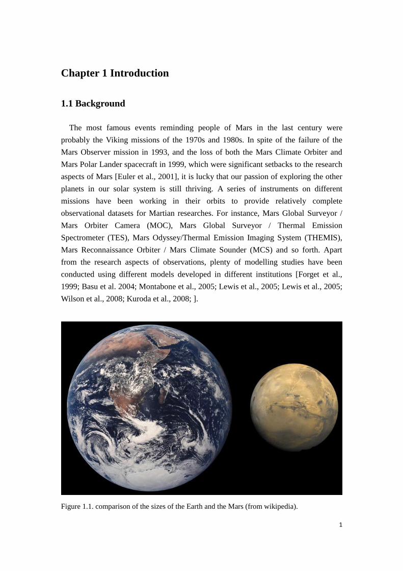
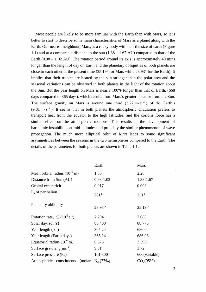
Figure 1.1. comparison of the sizes of the Earth and the Mars (from wikipedia).

2

Most people are likely to be more familiar with the Earth than with Mars, so it is

better to start to describe some main characteristics of Mars as a planet along with the

Earth. Our nearest neighbour, Mars, is a rocky body with half the size of earth (Figure

1.1) and at a comparable distance to the sun (1.38 – 1.67 AU) compared to that of the

Earth (0.98 – 1.02 AU). The rotation period around its axis is approximately 40 mins

longer than the length of day on Earth and the planetary obliquities of both planets are

close to each other at the present time (25.19° for Mars while 23.93° for the Earth). It

implies that their tropics are heated by the sun stronger than the polar area and the

seasonal variations can be observed in both planets in the light of the rotation about

the Sun. But the year length on Mars is nearly 100% longer than that of Earth, (668

days compared to 365 days), which results from Mars‟s greater distance from the Sun.

The surface gravity on Mars is around one third (3.72 2 sm ) of the Earth‟s

(9.81 2 sm ). It seems that in both planets the atmospheric circulation prefers to

transport heat from the equator to the high latitudes, and the coriolis force has a

similar effect on the atmospheric motions. This results in the development of

baroclinic instabilities at mid-latitudes and probably the similar phenomenon of wave

propagation. The much more elliptical orbit of Mars leads to some significant

asymmetrices between the seasons in the two hemispheres compared to the Earth. The

details of the parameters for both planets are shown in Table 1.1.

Earth Mars

Mean orbital radius (1011

m) 1.50 2.28

Distance from Sun (AU) 0.98-1.02 1.38-1.67

Orbital eccentricit 0.017 0.093

Ls of perihelion 281° 251°

Planetary obliquity 23.93° 25.19°

Rotation rate, (10-5

s-1

) 7.294 7.088

Solar day, sol (s) 86,400 88,775

Year length (sol) 365.24 686.6

Year length (Earth days) 365.24 686.98

Equatorial radius (106 m) 6.378 3.396

Surface gravity, g(ms-2

) 9.81 3.72

Surface pressure (Pa) 101,300 600(variable)

Atmospheric constituents (molar N2 (77%) CO2(95%)

3

ratio)

O2 (21%) N2(2.7%)

H2O(1%) Ar(1.6%)

Ar(0.9%) O2(0.13%)

Gas constant, R(m2s

-2K-

1) 287 192

cp/R 3.5 4.4

Mean Solar Constant (Wm-2

) 1367 589

Bond Albedo 0.306 0.25

Equilibrium temperature, Te (K) 256 210

Scale height, Hp=RTe/g (km) 7.5 10.8

Surface temperature (K) 230-315 140-300

Dry adiabatic lapse rate (K km-1

) 9.8 4.5

Buoyancy frequency, N(10-2

s-1

) 1.1 0.6

Deformation radius, pNHL

(km)

1100 920

Table 1.1, Parameters in the Earth and Mars (adapted from Read & Lewis (2004)).

Compared to the Earth, the Martian atmosphere is thin and composed mainly of

CO2 with small amounts of nitrogen (N2), argon (Ar) and very little oxygen (O2). The

total pressure of atmosphere on Mars is only 0.5%-1% that of the Earth. On Earth, the

water vapour makes the 1% of the atmospheric mass, while the concentrations of

water vapour is measured in precipitable microns, which means if all the water

contained in a vertical column of atmosphere were condensed to a liquid state, it

would form a layer typically only a few microns thick. Therefore, the Martian

atmosphere has very low absolute humidity. Actually, because of the low mean

pressure of the Martian atmosphere, close to that of the triple point of water, ice could

not melt into liquid water in most places but would sublime directly into water vapor

regardless of temperature below the normal freezing point of water (i.e., around 273 K

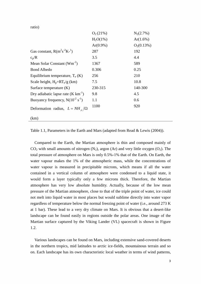
at 1 bar). These lead to a very dry climate on Mars. It is obvious that a desert-like

landscape can be found easily in regions outside the polar areas. One image of the

Martian surface captured by the Viking Lander (VL) spacecraft is shown in Figure

1.2.

Various landscapes can be found on Mars, including extensive sand-covered deserts

in the northern tropics, mid latitudes to arctic ice-fields, mountainous terrain and so

on. Each landscape has its own characteristic local weather in terms of wind patterns,

4

temperature and occasional clouds.

Figure 1.2 Viking Lander view of the Martian Surface (from http://mars.jpl.nasa.gov)

Apart from some similarities between Mars and Earth, dust is an extremely

important property on Mars. Martian atmospheric dust itself can strongly emit the

radiation in the infrared after absorbing short-wave solar radiation and also has great

capability of absorbing the long-wave surface radiation [Newman et al., 2002a].

Besides, there is a potential to develop dust storm on Mars locally and globally. Dust

particles can be lifted by near-surface wind stress and dust devils [Newman et al.,

2002a] so that some more dust can get into the dust cycle, and can settle back on the

Martian surface by the sedimentation mechanism. Thus, Martian dust has a

considerable impact on the thermal and dynamical state of the atmosphere.

The classification of dust storms in the report produced by Montabone et al. [2010]

will be described here. According to the classification based on a size-duration

relationship [Cantor et al., 2001], the types of dust storm can fall into three categories,

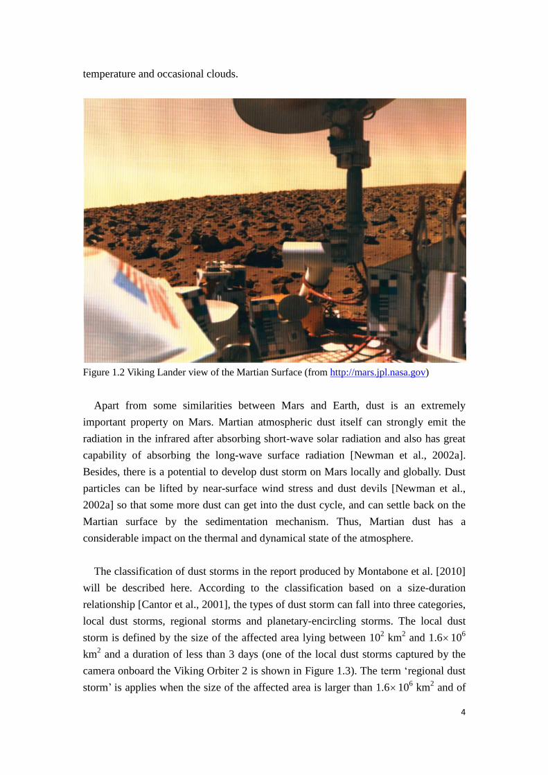
local dust storms, regional storms and planetary-encircling storms. The local dust

storm is defined by the size of the affected area lying between 102 km

2 and 1.610

6

km2 and a duration of less than 3 days (one of the local dust storms captured by the

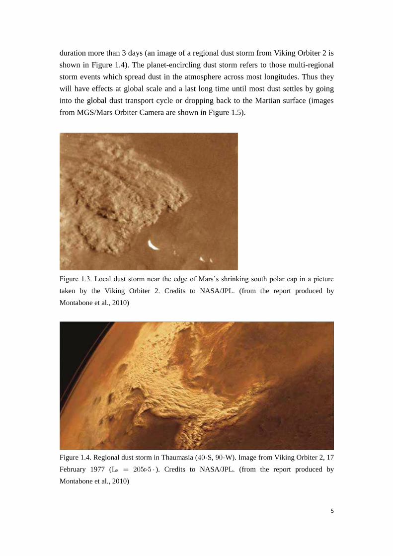
camera onboard the Viking Orbiter 2 is shown in Figure 1.3). The term „regional dust

storm‟ is applies when the size of the affected area is larger than 1.6106 km

2 and of

5

duration more than 3 days (an image of a regional dust storm from Viking Orbiter 2 is

shown in Figure 1.4). The planet-encircling dust storm refers to those multi-regional

storm events which spread dust in the atmosphere across most longitudes. Thus they

will have effects at global scale and a last long time until most dust settles by going

into the global dust transport cycle or dropping back to the Martian surface (images

from MGS/Mars Orbiter Camera are shown in Figure 1.5).

Figure 1.3. Local dust storm near the edge of Mars‟s shrinking south polar cap in a picture

taken by the Viking Orbiter 2. Credits to NASA/JPL. (from the report produced by

Montabone et al., 2010)

Figure 1.4. Regional dust storm in Thaumasia (40◦S, 90◦W). Image from Viking Orbiter 2, 17

February 1977 (Ls = 2055◦ ). Credits to NASA/JPL. (from the report produced by

Montabone et al., 2010)

6

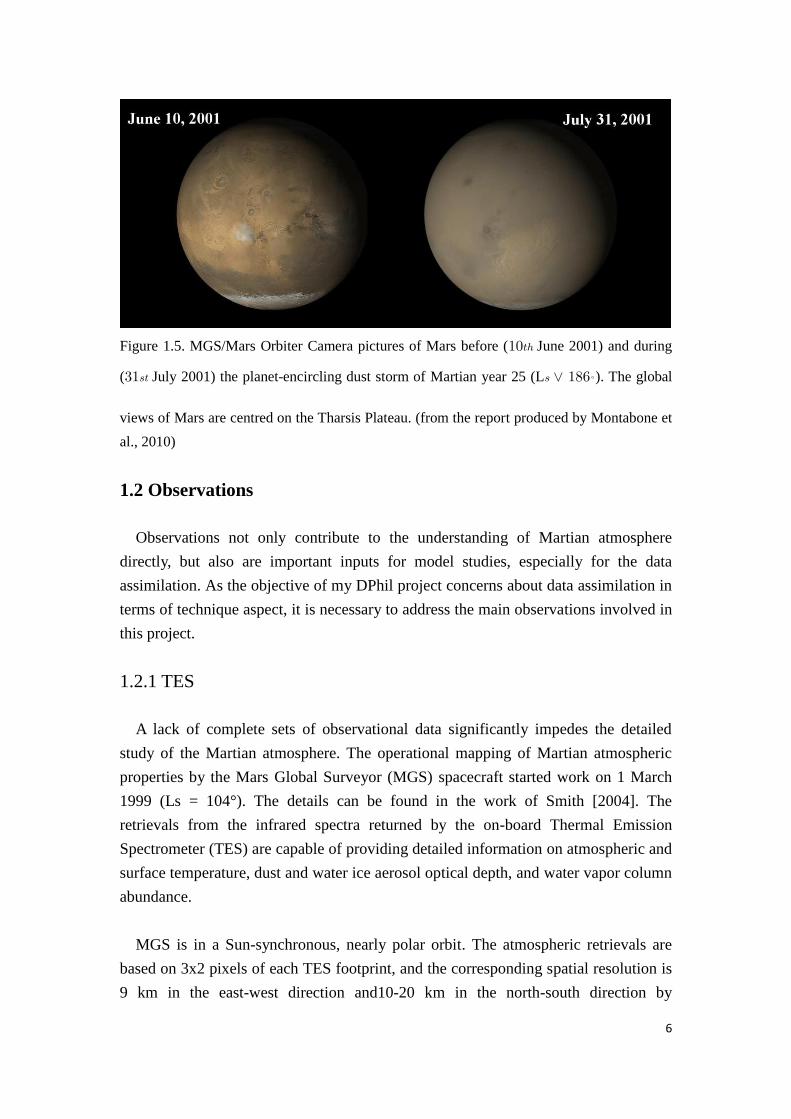
Figure 1.5. MGS/Mars Orbiter Camera pictures of Mars before (10June 2001) and during

(31July 2001) the planet-encircling dust storm of Martian year 25 (L_ 186◦). The global

views of Mars are centred on the Tharsis Plateau. (from the report produced by Montabone et

al., 2010)

1.2 Observations

Observations not only contribute to the understanding of Martian atmosphere

directly, but also are important inputs for model studies, especially for the data

assimilation. As the objective of my DPhil project concerns about data assimilation in

terms of technique aspect, it is necessary to address the main observations involved in

this project.

1.2.1 TES

A lack of complete sets of observational data significantly impedes the detailed

study of the Martian atmosphere. The operational mapping of Martian atmospheric

properties by the Mars Global Surveyor (MGS) spacecraft started work on 1 March

1999 (Ls = 104°). The details can be found in the work of Smith [2004]. The

retrievals from the infrared spectra returned by the on-board Thermal Emission

Spectrometer (TES) are capable of providing detailed information on atmospheric and

surface temperature, dust and water ice aerosol optical depth, and water vapor column

abundance.

MGS is in a Sun-synchronous, nearly polar orbit. The atmospheric retrievals are

based on 3x2 pixels of each TES footprint, and the corresponding spatial resolution is

9 km in the east-west direction and10-20 km in the north-south direction by

7

considering the impact of spacecraft motion. MGS provides two sets of twelve such

strips-like datasets each day, one of which set is taken near a local time of 1400 hours

and the other of which is taken near a local time of 0200 hours. A constrained linear

inversion of radiance in the 15- m CO2 band [Conrath et al., 2000] is used to

retrieve atmospheric temperature as a function of pressure. The uncertainty of

temperatures is ~2K in the middle atmosphere (~10-30km), and larger both in the

lowest scale height and at the highest altitudes where limb observation are used

[Smith, 2004].

After completing the retrieval of atmosphere temperature, the TES data team starts

to retrieve aerosol optical depth in a separate second step. The retrieval algorithm is

mainly based on the method used for Mars Odyssey THEMIS infrared data but with

further improvements [Smith, 2004]. The values of surface temperature, dust and

water ice optical depth which provide the best fit between computed and observed

radiance is the key output of the retrieval algorithm for aerosol optical depth. The

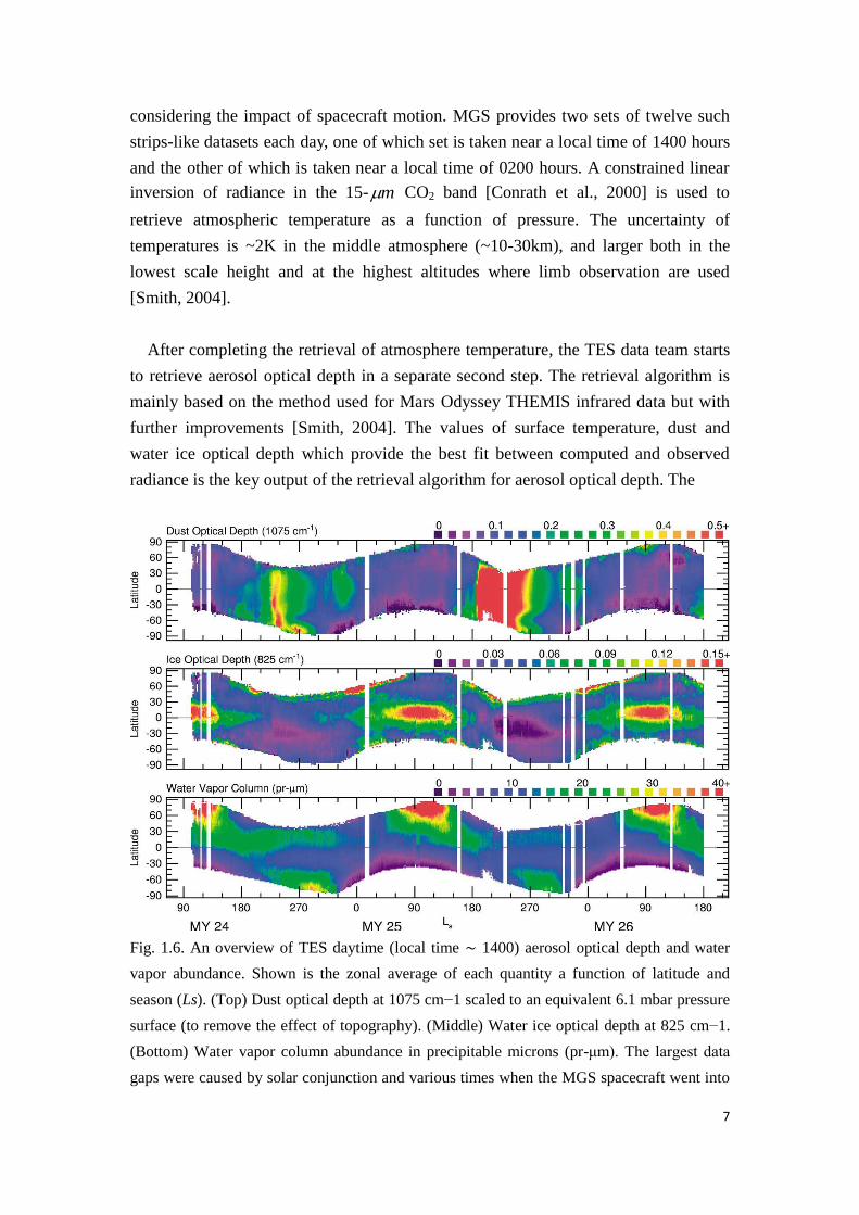
Fig. 1.6. An overview of TES daytime (local time ∼ 1400) aerosol optical depth and water

vapor abundance. Shown is the zonal average of each quantity a function of latitude and

season (Ls). (Top) Dust optical depth at 1075 cm−1 scaled to an equivalent 6.1 mbar pressure

surface (to remove the effect of topography). (Middle) Water ice optical depth at 825 cm−1.

(Bottom) Water vapor column abundance in precipitable microns (pr-μm). The largest data

gaps were caused by solar conjunction and various times when the MGS spacecraft went into

8

contingency (safing) mode.(from the work of Smith, 2004).

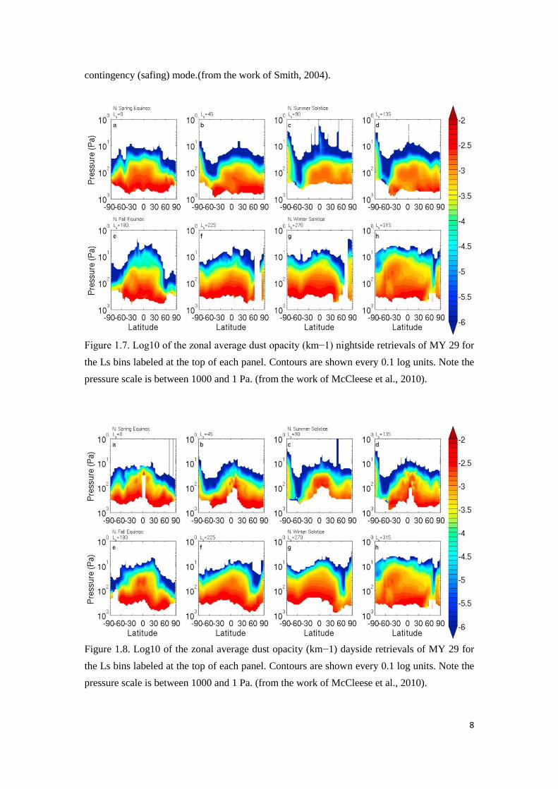
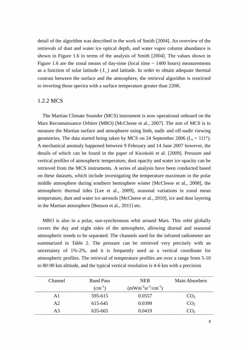
Figure 1.7. Log10 of the zonal average dust opacity (km−1) nightside retrievals of MY 29 for

the Ls bins labeled at the top of each panel. Contours are shown every 0.1 log units. Note the

pressure scale is between 1000 and 1 Pa. (from the work of McCleese et al., 2010).

Figure 1.8. Log10 of the zonal average dust opacity (km−1) dayside retrievals of MY 29 for

the Ls bins labeled at the top of each panel. Contours are shown every 0.1 log units. Note the

pressure scale is between 1000 and 1 Pa. (from the work of McCleese et al., 2010).

9

detail of the algorithm was described in the work of Smith [2004]. An overview of the

retrievals of dust and water ice optical depth, and water vapor column abundance is

shown in Figure 1.6 in terms of the analysis of Smith [2004]. The values shown in

Figure 1.6 are the zonal means of day-time (local time ~ 1400 hours) measurements

as a function of solar latitude ( sL ) and latitude. In order to obtain adequate thermal

contrast between the surface and the atmosphere, the retrieval algorithm is restricted

to inverting those spectra with a surface temperature greater than 220K.

1.2.2 MCS

The Martian Climate Sounder (MCS) instrument is now operational onboard on the

Mars Reconnaissance Orbiter (MRO) [McCleese et al., 2007]. The aim of MCS is to

measure the Martian surface and atmophsere using limb, nadir and off-nadir viewing

geometries. The data started being taken by MCS on 24 September 2006 (Ls = 111°).

A mechanical anomaly happened between 9 February and 14 June 2007 however, the

details of which can be found in the paper of Kleinbohl et al. [2009]. Pressure and

vertical profiles of atmospheric temperature, dust opacity and water ice opacity can be

retrieved from the MCS instruments. A series of analysis have been conducted based

on these datasets, which include investigating the temperature maximum in the polar

middle atmosphere during southern hemisphere winter [McCleese et al., 2008], the

atmospheric thermal tides [Lee et al., 2009], seasonal variations in zonal mean

temperature, dust and water ice aerosols [McCleese et al., 2010], ice and dust layering

in the Martian atmosphere [Benson et al., 2011] etc.

MRO is also in a polar, sun-synchronous orbit around Mars. This orbit globally

covers the day and night sides of the atmosphere, allowing diurnal and seasonal

atmospheric trends to be separated. The channels used for the infrared radiometer are

summarized in Table 2. The pressure can be retrieved very precisely with an

uncertainty of 1%-2%, and it is frequently used as a vertical coordinate for

atmospheric profiles. The retrieval of temperature profiles are over a range from 5-10

to 80-90 km altitude, and the typical vertical resolution is 4-6 km with a precision

Channel Band Pass

(cm-1

)

NER

(mWm-2

sr-1

/cm-1

)

Main Absorbers

A1 595-615 0.0557 CO2

A2 615-645 0.0399 CO2

A3 635-665 0.0419 CO2

10

A4 820-870 0.0287 H2O ice

A5 400-500 0.0278 Dust

B1 290-340 0.0453 Dust

B2 220-260 0.0568 H2O vapor, H2O

ice

B3 230-245 0.174 H2O vapor, H2O

ice

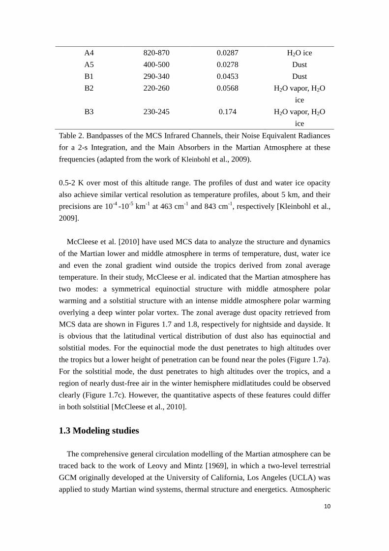
Table 2. Bandpasses of the MCS Infrared Channels, their Noise Equivalent Radiances

for a 2-s Integration, and the Main Absorbers in the Martian Atmosphere at these

frequencies (adapted from the work of Kleinbohl et al., 2009).

0.5-2 K over most of this altitude range. The profiles of dust and water ice opacity

also achieve similar vertical resolution as temperature profiles, about 5 km, and their

precisions are 10-4

-10-5

km-1

at 463 cm-1

and 843 cm-1

, respectively [Kleinbohl et al.,

2009].

McCleese et al. [2010] have used MCS data to analyze the structure and dynamics

of the Martian lower and middle atmosphere in terms of temperature, dust, water ice

and even the zonal gradient wind outside the tropics derived from zonal average

temperature. In their study, McCleese er al. indicated that the Martian atmosphere has

two modes: a symmetrical equinoctial structure with middle atmosphere polar

warming and a solstitial structure with an intense middle atmosphere polar warming

overlying a deep winter polar vortex. The zonal average dust opacity retrieved from

MCS data are shown in Figures 1.7 and 1.8, respectively for nightside and dayside. It

is obvious that the latitudinal vertical distribution of dust also has equinoctial and

solstitial modes. For the equinoctial mode the dust penetrates to high altitudes over

the tropics but a lower height of penetration can be found near the poles (Figure 1.7a).

For the solstitial mode, the dust penetrates to high altitudes over the tropics, and a

region of nearly dust-free air in the winter hemisphere midlatitudes could be observed

clearly (Figure 1.7c). However, the quantitative aspects of these features could differ

in both solstitial [McCleese et al., 2010].

1.3 Modeling studies

The comprehensive general circulation modelling of the Martian atmosphere can be

traced back to the work of Leovy and Mintz [1969], in which a two-level terrestrial

GCM originally developed at the University of California, Los Angeles (UCLA) was

applied to study Martian wind systems, thermal structure and energetics. Atmospheric

11

condensation of CO2 and the presence of transient baroclinic waves in the winter

mid-latitudes were simulated by this model. From the early 1970s, further model

development was conducted continually at NASA‟s Ames Research Center, resulting

in a model known as the NASA Ames Mars GCM. With the topographic data released

from Mariner 9 measurements, the NASA Ames Mars GCM started to include

spatially varying surface elevation at the model‟s lower boundary. The first 3-D

simulations of a global dust storm were conducted with the Ames Mars GCM

incorporating a tracer transport scheme [Murphy et al., 1995]. The important role of

dust transport by atmospheric eddies and the seasonal and topographic effects

resulting in the differences in each hemisphere were illustrated in their work, as well

as the Martian polar warming and the relationship between CO2 column loading and

the onset of major dust storms.

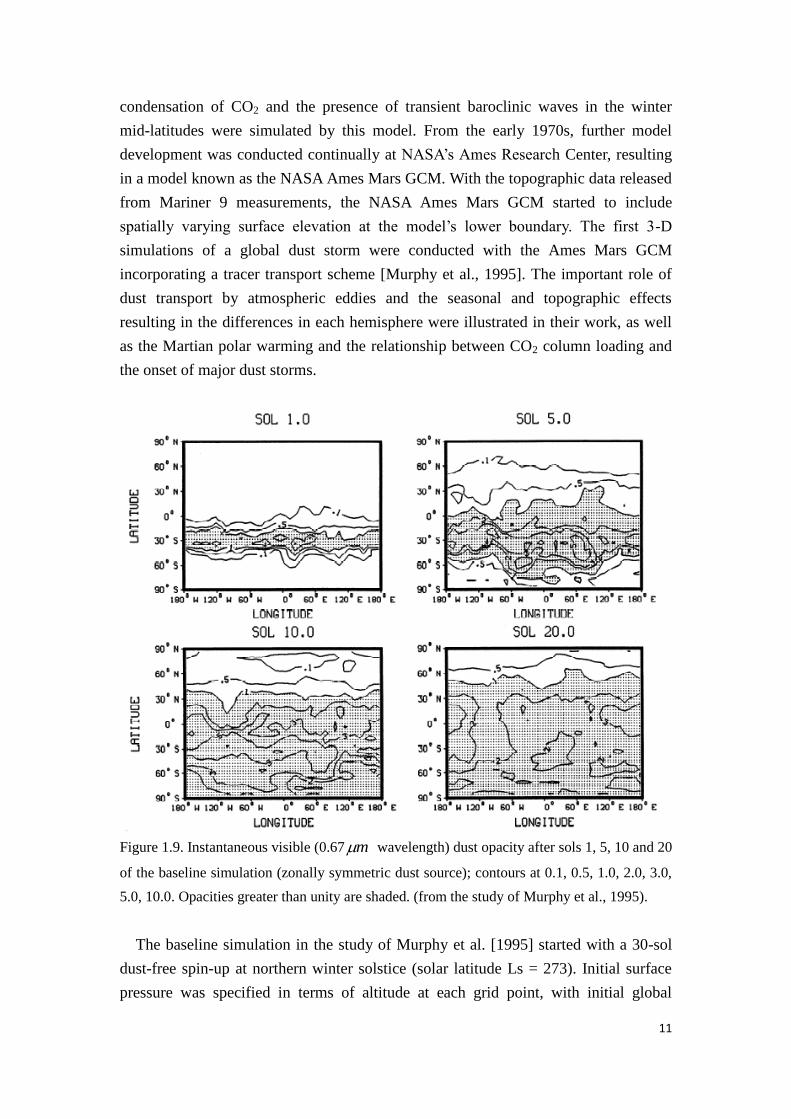
Figure 1.9. Instantaneous visible (0.67 m wavelength) dust opacity after sols 1, 5, 10 and 20

of the baseline simulation (zonally symmetric dust source); contours at 0.1, 0.5, 1.0, 2.0, 3.0,

5.0, 10.0. Opacities greater than unity are shaded. (from the study of Murphy et al., 1995).

The baseline simulation in the study of Murphy et al. [1995] started with a 30-sol

dust-free spin-up at northern winter solstice (solar latitude Ls = 273). Initial surface

pressure was specified in terms of altitude at each grid point, with initial global

12

average values of 7.6 mbar. After spin-up, the MGCM was coupled with an aerosol

model (described in detail in their work) interactively. They prescribed a uniform dust

source in the aerosol model on the entire surface between the 15°S and 37.5°S

[Murphy et al., 1995]. The source magnitude was 1.5410-7

kgm-2

s-1

for 10 sols with

a prescribed size distribution and a particle material density of 3000kg m-3

[Toon et

al., 1977]. The simulation was conducted for an additional 40 sols after steady dust

injection for 10 sols. In their baseline simulation (see Figure 1.9), the dust spread all

over the domain except the northern polar region at a rapid pace (by 20 sols, see

Figure 1.9d). The 1vis line moves to 10°N by sol 5 (Figure 1.9a), then to about

40°N by sol 10. By sol 20 (Figure 1.9d), the dust had reached 50°N and the spread of

dust was much faster moving to the south from the original dust source region

prescribed in this study. The optical depth higher than 1vis line could almost

cover the southern hemisphere by sol 20 (Figure 1.9d). The dust distribution

developed very asymmetrically within the south of the dust input corridor (Figure

1.9b, c) and they claimed that this strong southward transport was due primarily to a

strong standing eddy that developed rapidly during the dust input phase of the

simulation and rapidly diminished after sol 5. However, in their parallel simulation

the same as this baseline simulation but with spatially invariant topography, thermal

inertia and albedo fields, this southward dust transport was not so strong as in the

baseline simulation. However, at that time, there was not enough observational data to

verify their model simulations directly.

In 1989 the grid-based LMD (Laboratoire de Météorologie Dynamique) Martian

GCM was developed on the basis of the LMD terrestrial climate model, which was

used on earth for weather forecasting or climate change studies [Forget et al., 1999]. A

new radiative transfer code and a self-consistent parameterization for the

condensation and sublimation of CO2 were developed to adapt to the Martian

atmospheric conditions. Reasonable seasonal and transient pressure variations were

able to be reproduced by this model, the first to simulate a full Martian year without

any forcing other than insolation. [Hourdin et al., 1995; Collins et al., 1996].

Around this time, a GCM with a physical package similar to the Ames model was

developed at the Geophysical Fluid Dynamic Laboratory (GFDL), Princeton, USA.

The GFDL Mars GCM was adapted from the GFDL Skyhi GCM [Hamilton, 1995;

Wilson and Hamilton, 1996]. The model has since been used to study many different

phenomena on Mars, such as Martian thermal tides [Wilson and Hamilton, 1996],

surface winds [Fenton and Richardson, 2001] and dust cycle [Basu et al., 2004]. In the

study of Basu et al. [2004], they mainly investigated the capability of simulating the

13

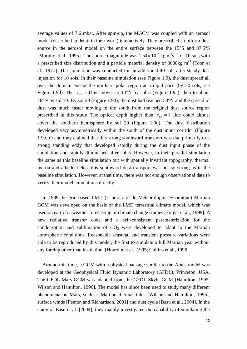
dust cycle and related temperature fields by the GFDL Mars GCM with a similar

approach to treating dust lifting as described in the work of Newman et al. [2002a].

Through their model experiments, they obtained a set of parameters to provide a “best

fit” model climate based on Dust Devil lifting responsible for the seasonal haze cycle

and Wind Stress lifting responsible for dust storms. For a year without a major dust

storm, the comparison between observations and temperature fields predicted by their

model in terms of “best fit” tuning is shown in Figure 1.10. From Figure 1.10 a and b,

it indicates that not only had “global mean” temperatures been produced reasonably,

but also the meridional gradients. Specifically, the double-peak feature of air

temperatures in the mid-latitudes in both hemispheres, and local minimum in the

tropics during summer could be observed in their model results. In Figure 1.10c, the

difference between the GCM output and the TES observations suggested that their

Figure 1.10. A comparison of zonal-mean 15 mm channel temperatures derived from the

MGS TES spectra and from the GCM. The GCM output was sampled using the TES

observational pattern to maximize comparability. A full annual cycle is shown for each, along

with the difference between the model and data. The results are for a nonglobal dust storm

year (the first MGS mapping year from northern summer and rolling around into the second)

and from the „„best fit‟‟ GCM simulation. (from the work of Basu et al., 2004)

14

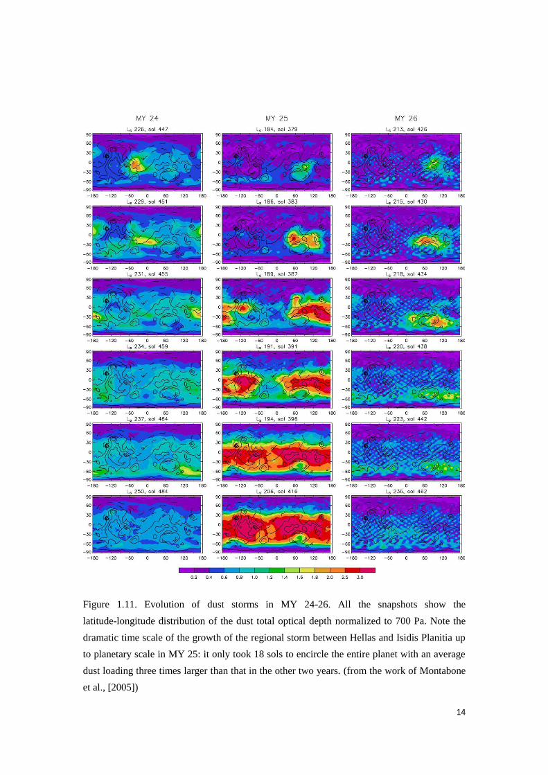
Figure 1.11. Evolution of dust storms in MY 24-26. All the snapshots show the

latitude-longitude distribution of the dust total optical depth normalized to 700 Pa. Note the

dramatic time scale of the growth of the regional storm between Hellas and Isidis Planitia up

to planetary scale in MY 25: it only took 18 sols to encircle the entire planet with an average

dust loading three times larger than that in the other two years. (from the work of Montabone

et al., [2005])

15

model predicted the air temperature in the mid-latitudes and tropics quite well except

the relatively large discrepancy at roughly 200sL and 235sL . However, for

the polar region, large discrepancy ( 20 ) could be seen in both hemispheres,

especially for the southern hemisphere.

Almost at the same time, in the 1990s, a three-dimensional Martian GCM (MGCM)

was developed jointly with University of Reading and Oxford in the United Kingdom.

The spectral solver used in this MGCM was originally adapted from University of

Reading [Hoskins and Simmons, 1975]. But in the vertical direction, levels were still

defined in terms of the terrain-following coordinate system using a standard finite

difference approach. Besides simulating the standard atmospheric properties, the UK

MGCM also has the capability (shared with the LMD MGCM since the mid 1990s) of

treating the CO2, water and dust cycles, CO2-ice transformation, as well as data

assimilation for temperature and dust [Montabone et al., 2005; Lewis et al., 2005;

Montabone et al., 2006a; Montabone et al., 2006b; Lewis et al., 2007; Wilson et al.,

2008; Rogberg et al. 2010]. In the work of Montabone et al. [2005], data assimilation

for temperature profiles and total dust opacity was employed to provide the best-fit

model outputs. Not only was the interannual variability of different atmospheric

properties described, but also the evolution of dust storm in Martian year (MY) 24-26

(see Figure 1.11), including the 2001 planet-encircling dust storm (occurred in

MY25). In their study, they pointed out that the localization of major dust storms

varied with season. The 2001 planet-encircling dust storm started as a regional storm

but developed to a planetary-scale dust storm only within 18 sols because of the

eastward migration and the consequent contribution of dust from the Tharsis region

and the plains south of the Tharsis ridge. This probably resulted from the positive

feedback of the strength of wind stress lifting because of radiative interactions with

the dust cloud, which would enhance the dust lifting in turn. In fact, in MY26, some

regional storms built up in the same place as at the start of the MY 25 global storm,

but did not develop strongly enough to form a planetary-scale dust storm.

1.4 Motivation and objectives

Dust is now included in almost all current state-of-the-art Martian GCMs in some

form. The dust in the Martian model simulations is generally treated in one of several

different ways: either

1) treating dust as prescribed in seasonal and latitudinal dust distribution scenarios

in terms of available observations and then repeated in other years, such as the TES

16

scenario in the study of Kuroda et al., 2008,

2) assuming the dust opacity is horizontally and temporally uniform at a certain

reference level (typically 6.1 mbar), and then distributing the dust according to the

prescribed vertical profile originally described by Conrah [1975] [Kahre and Haberle,

2010],

3) before transporting the dust in terms of the wind fields and temperature predicted

by Martian GCM itself, giving an initial prescribed injection of dust [Murphy et al.,

1995],

4) simulating dust transport using the wind fields and temperature predicted by the

Martian GCM itself, but with runtime dust sources, i.e. near-surface wind stress lifting

and dust devil lifting [Newman et al., 2002a; Basu et al., 2004] or,

5) data assimilation for observed column dust opacity without dust transport, and

distributing the dust vertically by scaling of a prescribed (Conrath) profile

[Montabone et al., 2005; Lewis et al., 2007].

The methods mentioned above have their own advantages and disadvantages.

Method 1) only has reliable information for the column dust opacity according to the

limitation of TES observations. Even if vertical information is available in the

observed datasets, such as, in MCS limb data, it will still lose the detailed information

in space, as well as any annual variability. Method 2) is based on the various idealised

assumptions like horizontally and temporally uniform dust opacity and empirically

determined vertical dust distributions [Kahre and Haberle, 2010], so it is almost

impossible to represent real instantaneous atmospheric conditions. In the method 3) a

totally artificial dust source is added at the start of the simulation so that it lacks of the

representation of dust lifting mechanisms on Mars and can not therefore make the

results physically and numerically reasonable after a relatively long-term simulation.

In this case the dust would either spread across most of the planet ( as shown in the

results of Murphy et al. [1995]) which may not be realistic or possibly settle out by

sedimentation. Method 4) has reasonable physical mechanisms to represent the unique

dust behaviours on Mars and can therefore produce results in acceptable agreement

with real observations. However, no simulation has yet produced the observed amount

of interannual variability [Newman et al., 2002b]. Finally, method 5) was able to

provide a complete and balanced “best-fit” to the observations, but the dust transport

has not been enabled so far because of a lack of vertical information on dust opacity

from TES. Thus, the dust would be distributed by scaling the Conrath profile in the

vertical and remains static when no observation is available to correct the dust fields.

As discussed above, method 4) should be the most reasonable way of doing dust

17

simulation on Mars in terms of its physical representation. However, in the light of

data and model [Newman et al., 2002a; Newman et al., 2002b] limitations, it is

difficult to understand the dust behaviour precisely, which results in a failure to

produce some significant features of dust storms, (e.g. the development of 2001

planet-encircling dust storm), as well as the interannual variability of dust. Method 5,

on the other hand, in practice generates results that are a “best-fit” to real observations

through the data assimilation technique, because of data limitation, absence of a dust

transport scheme leads to an unrealistic vertical distribution of dust. This impedes the

progress of the research related to the dust, and the capability of providing a realistic

reconstruction of the dust storm structures, especially for the 2001 planet-encircling

dust storm.

Therefore, it is extremely important to improve the capability of the data

assimilation technique on Mars. As MCS datasets become available which contain

vertical information on dust opacity, it should be entirely possible to incorporate the

dust transport scheme into the data assimilation technique in order to provide a

three-dimensional structure of dust storms, corrected by the real observational data.

In this project, the UK Martian GCM will be used as a primary tool to develop

more advanced data assimilation scheme for temperature and dust. The aim of this

project is to incorporate the data assimilation scheme and the dust transport scheme

into the model integration together in a new version of the MGCM. For the data

assimilation scheme itself, we will extend the assimilation of column dust opacity to

include the capability of assimilating dust profiles, similar to that done for

temperature profile in the current model setting.

With this new development of MGCM data assimilation, UK MGCM will be a

powerful tool to investigate dust activity on Mars. Corrected opacities will be

appropriately converted to dust mixing ratios, and further used to reconstruct the dust

transport and diagnose the degree to which it is predicted in the model. It will be able

to provide three-dimensional information on the dust distribution for the further study

of the evolution of dust storms, as well as the atmospheric properties affected by dust

storms. What is more, it will provide insight to investigate the interannual and

interseasonal variability of Martian climate. It also offers possibility of improving the

dust lifting schemes themselves. Given that the temperatures and winds are basically

correct in the reanalysis, the correction of the dust field becomes solely a test of the

accuracy of lifting parameterizations, as well as the assumptions about surface dust

availability. To some more extent, this study can perhaps also provide information

18

towards planning the future Exomars Climate Sounder (EMCS) investigation

[Schofield et al., 2011], as well as other possible applications of the observational

data.

19

Chapter 2 Martian General Circulation Model

A three-dimensional Martian General Circulation Model (MGCM) has been used to

study the Martian Atmosphere [Forget et al., 1999]. Further, based on this MGCM,

data assimilation has been applied in several studies [Montabone et al., 2005; Lewis et

al., 2005; Montabone et al., 2006a; Montabone et al., 2006b; Lewis et al., 2007;

Wilson et al., 2008; Rogberg et al. 2010] as an effective tool with which to analyze

spacecraft observations and phenomena (e.g., atmospheric tides, transient wave

behavior, effects of clouds in the tropics, weather predictability, etc.) in the Martian

atmosphere. The MGCM employed in my study combines a spectral dynamical solver

and a tracer transport scheme developed in UK and Laboratoire de Météorologie

Dynamique (LMD; Paris, France) physics package developed in collaboration with

Oxford, The Open University and Instituto de Astrofisica de Andalucia (Granada,

Spain).

In this chapter, the details of MGCM will be described, for instance, model

dynamics, physics parameterizations and so forth. Besides, the description of data

assimilation scheme, which has been implemented in the MGCM, is included as well.

2.1 Model Dynamics

The dynamical core of our MGCM is based on a spectral solver which was adapted

from University of Reading [Hoskings and Simmons, 1975]. With further extension,

the total wavenumber for triangular truncation is 31 corresponding to 3672 real

space grids in longitude latitude.

In the vertical direction, levels are defined in terms of the terrain-following

coordinate system using a standard finite difference approach. The first three of 25

vertical levels close to surface are at heights of 4, 19 and 44 m above surface, and this

enhanced vertical resolution near the surface provides the capability of resolving

detailed surface processes represented in the model. The middle of the top layer is at

an altitude of 80 km. Some advantages coming with this extension are that it enables

us to explore the meteorological phenomenon at higher altitudes and such a deeper

model domain allows the unconstrained development of the Hadley circulation and is

important to obtain a better simulation [Forget et al., 1999]. At the three uppermost

levels, sponge layers are used with the purpose of reducing the spurious reflections of

vertically propagating waves from the model top. A linear drag is added to the eddy

20

components of the vorticity and divergence fields.

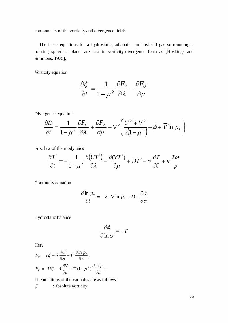
The basic equations for a hydrostatic, adiabatic and inviscid gas surrounding a

rotating spherical planet are cast in vorticity-divergence form as [Hoskings and

Simmons, 1975],

Vorticity equation

UV FF

t 21

1

Divergence equation

*2

222

2ln

121

1pT

VUFF

t

D VU

First law of thermodynaics

p

TTTD

TVTU

t

T

)(

1

12

Continuity equation

DpV

t

p*

* lnln

Hydrostatic balance

T

ln

Here

*ln p

TU

VFU ,

*2 ln

)1(p

TV

UFV .

The notations of the variables are as follows,

: absolute vorticity

21

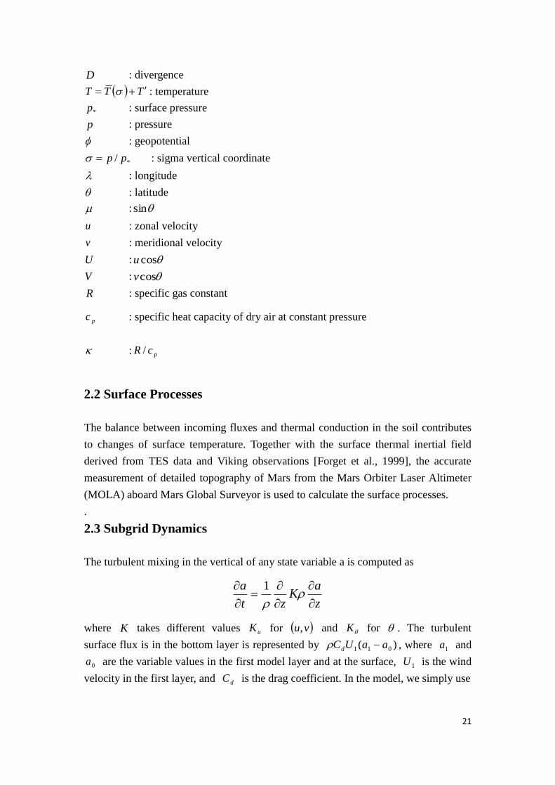
D : divergence

TTT : temperature

*p : surface pressure

p : pressure

: geopotential

*/ pp : sigma vertical coordinate

: longitude

: latitude

: sin

u : zonal velocity

v : meridional velocity

U : cosu

V : cosv

R : specific gas constant

pc : specific heat capacity of dry air at constant pressure

: pcR /

2.2 Surface Processes

The balance between incoming fluxes and thermal conduction in the soil contributes

to changes of surface temperature. Together with the surface thermal inertial field

derived from TES data and Viking observations [Forget et al., 1999], the accurate

measurement of detailed topography of Mars from the Mars Orbiter Laser Altimeter

(MOLA) aboard Mars Global Surveyor is used to calculate the surface processes.

.

2.3 Subgrid Dynamics

The turbulent mixing in the vertical of any state variable a is computed as

z

aK

zt

a

1

where K takes different values uK for vu, and K for . The turbulent

surface flux is in the bottom layer is represented by )( 011 aaUCd , where 1a and

0a are the variable values in the first model layer and at the surface, 1U is the wind

velocity in the first layer, and dC is the drag coefficient. In the model, we simply use

22

2

0

ln

z

zCd

here, represents the von Karman constant, which is assumed to take the value 0.4

and 0z is the roughness coefficient which is chosen to be 0.01 m everywhere on

Mars suggested by Sutton et al. [1978] for the Viking Lander sites.

Based on an equation for evolution of the turbulent kinetic energy (TKE) [ Mellor and

Yamada, 1982], the mixing coefficients are computed. The evolution of TKE can be

obtained from

z

EK

zbGSGS

l

q

t

EEuu

1

3 1

where,

Eq 2

22

z

v

z

uM

2

2

2

Mq

lGu

z

g

q

lG

0

2

2

GG

GSu

43

21

11

GS

3

5

1

6ES

The coefficients 1 , 2 , 3 , 4 , 5 , 6 , 1b are assigned the constant values

0.393, -3.09, -34.7, -6.13, 0.494, 0.38, 16.6 [Forget et al., 1999].

2.4 Dust lifting mechanisms

2.4.1 Dust lifting by near-surface wind stress

23

The vertical flux of lifted dust NV is assumed to be proportional to the horizontal

saltation flux of sand [Montabone et al., 2005]:

2

3

2

1

2

1

2

31

ttNV

where represents the near-surface air density, represents the near-surface wind

stress magnitude and t represents an empirically determined stress threshold for the

lifting to occur. The near-surface wind stress is related to the near-surface wind

speed U by,

2

0/ln

zz

zU

where represents von Karman‟s constant, z is the average height of the lowest

layer above the surface and 0z is the height at which velocities are zero (i.e.

roughness height, taken as 0.01m everywhere on Mars).

2.4.2 Dust lifting by the activity of dust devils

The flux of dust lifted by the activity of dust devils (i.e. the thermodynamic

efficiency of the dust devil convective heat engine) is obtained by

stops

tops

ppp

pp

11

11

,

where sp represents the surface pressure, topp represents the pressure at the top of

the convective boundary layer (defined in the model where TKE drops down to a

threshold of 0.5 22 sm ), and represents the specific gas constant divided by the

specific heat capacity at constant pressure. The energy to drive any dust devil is

determined by the temperature difference of surface to air, while the thermodynamic

efficiency relate to how high the dust devils are able to grow [Rennó et al., 1998].

2.5 Data assimilation

A data assimilation scheme combined with a Martian Global Circulation Model

(MGCM) is able to provide a complete, balanced, four-dimensional solution

consistent with observations. This technique has been applied in several previous

studies to give us a better understanding of phenomena in the Martian atmosphere

given incomplete and/or noisy measurements [Montabone et al., 2005; Lewis et al.,

24

2005; Montabone et al., 2006a; Montabone et al., 2006b; Lewis et al., 2007; Wilson et

al., 2008; Rogberg et al. 2010]

The data assimilation scheme implemented in the MGCM is computationally

inexpensive compared to MGCM itself, and based on the analysis correction

sequential estimation scheme [Lorenc et al., 1991], but with modifications specific to

Mars [Lewis et al., 2007].

The analysis iteration, which is based on the least-squares sense, is performed at

each dynamical time step of the model (currently 480 times per sol at the chosen

resolution), and attempts to make the model predictions fit to the observations in

terms of their relative errors. Observational increments to the model are determined in

time and space in terms of empirical covariance functions.

For the current study, only temperature profiles and measurements of total dust

opacity have so far been assimilated into the MGCM at each horizontal grid point.

After the analysis correction of the temperature field, the temperature increments are

balanced by non-divergent, thermal wind increments. Thus, the wind fields will be

adjusted slightly consistent with the geostrophic thermal wind balance.

The analysis correction of temperature profiles was performed in the vertical

direction followed by the horizontal and temporal analysis. The temperatures are

interpreted as mean temperatures between a standard set of pressure values, which can

represent the resolution of the vertical temperature retrievals. The corresponding

model layer thickness is calculated between each pressure value in terms consistent

with the temperature retrievals. The philosophy behind this method is that the vertical

scale of temperature increments should reflect the observational resolution instead of

the model vertical resolution. This method also has the advantage of maintaining

detailed features in the vertical direction which are predicted by the dynamics and

physics of the model itself, even if this can not be resolved explicitly by the

remotely-sensed data.

In the horizontal space, the increments to the model variables on each model grid,

kx are spread by the following function [Lorenc et al., 1991],

where,

i

iiiikik CtRQx 2

25

k : refers to a model grid point

i : refers to an observation

iQ : is a function of the ratio of observational to first guess error and of the local

observation density around each observation location.

2

iR : is a function used to determine how the observational increments are spread in

time

t : is the time difference between model time and observation time (see Figure 2.1).

iC : is the increments at the observation locations.

and ki will be explained in detail afterwards.

In practice, the model will read in the observation data 5h before they are valid and

finally discards them 1 h after their valid time.

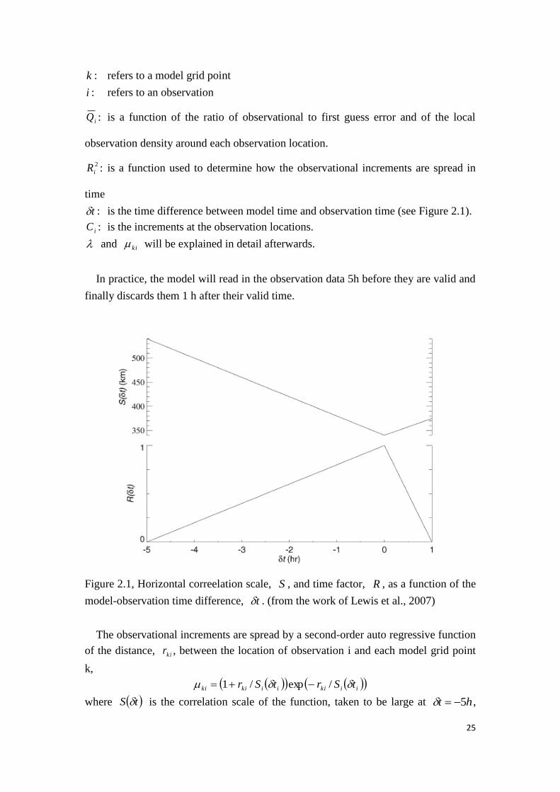
Figure 2.1, Horizontal correelation scale, S , and time factor, R , as a function of the

model-observation time difference, t . (from the work of Lewis et al., 2007)

The observational increments are spread by a second-order auto regressive function

of the distance, kir , between the location of observation i and each model grid point

k,

iikiiikiki tSrtSr /exp/1

where tS is the correlation scale of the function, taken to be large at ht 5 ,

26

and a minimum at ht 0 . Overall, the increment will reduce by a factor of half over

nearly 570 km distance, but the maximum radius of influence is chosen at 1200 km.

The parameter is related to the nudging relation with nudging coefficient G

by

tG 1/

Here, t is the model dynamical time step. G was set to 14105 s with a linear

reduction, between 30 and 20 latitude in both hemispheres to 14104 s at equator.

However, in the current model setup, data assimilation of total dust opacity is only

conducted without advecting the dust mainly because it is to simplify the first attempt

to take dust variations into account. Therefore, the vertical distribution of the dust

opacity tau at the given latitude, longitude and time is determined by an empirical

relation of the form,

max

01expzb

ppataureftau

For pressure 0pp , where 0p is taken to be Pap 7000 , and with tautauref ,

for 0pp , tauref is the total dust opacity at reference level (700 Pa), latitude,

longitude and time. a and b are constant with values 007.0a , kmb 70 . m axz is

the „top‟ of the dust layer, varying with solar longitude sL and latitude

determined by

sin160sin8160sin1832sin160sin1860 4

max sss LLLz

In the new work described in this report, the assimilation of dust measurements has

been extended to allow for the advection of dust by the winds simulated by the model.

The details of recent development for combining the dust transport and the

assimilation of total dust opacity will be addressed in the chapter 4 (2-D Data

Assimilation of Column Dust Opacity with Dust Transport).

27

Chapter 3 Interannual and Interseasonal Variability of

Martian Climate using Data Assimilation: A Semi-Annual

Oscillation

In the upper stratosphere and mesosphere of Earth, the semi-annual oscillation

(SAO) of the mean zonal wind in the tropical stratosphere and mesosphere is found as

a clear feature [Reed, 1966; Garcia et al., 1997]. Reed [1966] used observational data

to study the semi-annual cycle of zonal wind on Earth. He pointed out that the

strongest westerly winds occur shortly after the equinoxes in the lower mesosphere

and later extended to the lower levels. The pronounced semi-annual oscillation

happens at intermediate and upper levels, and the amplitude of the semi-annual

component reaches a peak at about the height of the stratopause. Similar features in

the Martian tropics (between 10°S and 10°N) have been studied in the work of

Kuroda et al. [2008]. Here, we are going to present some actual observations of the

SAO phenomenon on Mars derived from assimilated model (MGCM) results, but in

contrast to the study of Kuroda et al., extended to the atmosphere of the whole planet.

We divide the atmosphere into 7 latitude bands (60°N and 90°N, 40°N and 60°N,

10°N and 40°N, 10°S and 10°N, 10°S and 40°S, 40°S and 60°S, 60°S and 90°S). In

each latitude band, not only will the actual zonal-mean of daily-averaged zonal wind

be presented and discussed in this chapter, but also the results of a singular Spectrum

Analysis (SSA) of daily averaged zonal-mean zonal wind, including the amplitudes of

the first 6 Principal Components (PCs) evolving with time, corresponding eigenvector

height-time contour maps which isolate and capture the semi-annual oscillation

component and reconstructions of the magnitude of semi-annual oscillation

components will be analyzed.

3.1 Previous work on semi-annual oscillations on Mars

In the work of Kuroda et al. [2008], a clear SAO phenomenon between 10°S and

10°N, similar to the stratospheric SAO in the Earth in terms of appearance, is

described in their results from a free-running Martian General Circulation Model

(GCM; see Figure 3.1 for their results of semi-annual oscillation). Their simulations

were run for 7 model Martian years initialized from an initial isothermal and windless

state, and the last 5 years output were used to conduct their study on Martian

semi-annual oscillations.

28

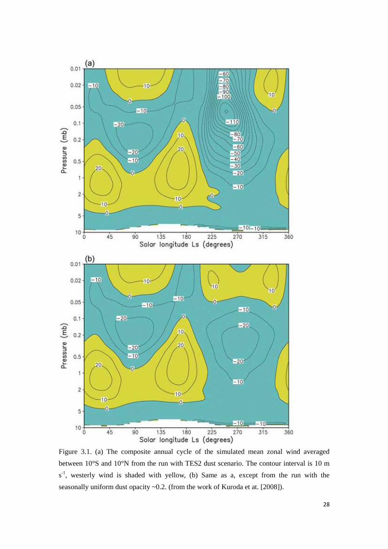
Figure 3.1. (a) The composite annual cycle of the simulated mean zonal wind averaged

between 10°S and 10°N from the run with TES2 dust scenario. The contour interval is 10 m

s-1

, westerly wind is shaded with yellow, (b) Same as a, except from the run with the

seasonally uniform dust opacity ~0.2. (from the work of Kuroda et at. [2008]).

29

Two scenarios were conducted by Kuroda et al. [2008] to demonstrate the

semi-annual oscillation on Mars. One was run with a prescribed dust opacity

representing the MGS-TES retrievals (shown in Figure 3.1a), and the other was run

with a seasonally uniform dust opacity (~0.2; Figure 3.1b). Afterwards, the simulated

zonal wind was averaged between 10°S and 10°N temporally and horizontally to

obtain the mean annual cycle.

In Figure 3.1a, it is seen that a clear semi-annual oscillation feature can be observed

in the middle atmosphere especially between 0.2 and 1mb. In the first quarter of the

year, the mean zonal wind changes from westerly to easterly between 0.2-1mb, or the

westerly component increases in some altitudes. During the second quarter of the year,

the mean zonal wind changes back to easterly in the corresponding altitudes, or the

westerly component decreases. Thus, a full cycle of a semi-annual oscillation

completes, and a new cycle will start. However, on comparing the two cycles within

one year, it seems that the oscillation in the second half year is stronger in terms of the

zonal wind gradient and penetration in the vertical direction. In the other scenario

(Figure 3.1b), in which the simulation is repeated with seasonally uniform dust

opacity, a similar semi-annual oscillation can be seen but with relatively equal

magnitude in the second half year compared to the scenario with MGS-TES dust

variations.

3.2 Study of semi-annual oscillation with our MGCM

In this section, we present actual observations (nearly 3 Martian years in total) of

SAO phenomena on Mars derived from assimilated model results in different latitude

bands (60°N and 90°N, 40°N and 60°N, 10°N and 40°N, 10°S and 10°N, 10°S and

40°S, 40°S and 60°S, 60°S and 90°S) which are based on a reanalysis using the UK

MGCM with a data assimilation scheme which assimilates Mars Global

Surveyor/Thermal Emission Spectrometer (MGS/TES) retrievals of temperature and

column dust opacity. The detailed model setup was described in Chapter 2, and the

data assimilation scheme employed in this study was introduced in the work of Lewis

et al.[2007]. The pressure and pseudo-altitude values in the following figures are

simply calculated from the model terrain-following vertical sigma coordinate using a

reference pressure of 6.1mb and a scale height of 10.8km.

In the same latitude band (10°S and 10°N) that was chosen to discuss the

semi-annual oscillation in the work of Kuroda et al. ([2008]; Figure 3.1), a similar

semi-annual oscillation phenomenon can be observed in our 3-year results (left panel

30

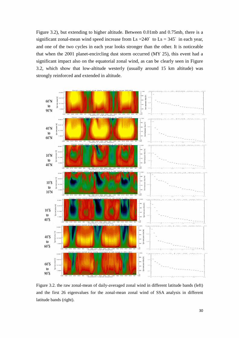
Figure 3.2), but extending to higher altitude. Between 0.01mb and 0.75mb, there is a

significant zonal-mean wind speed increase from Ls =240° to Ls = 345° in each year,

and one of the two cycles in each year looks stronger than the other. It is noticeable

that when the 2001 planet-encircling dust storm occurred (MY 25), this event had a

significant impact also on the equatorial zonal wind, as can be clearly seen in Figure

3.2, which show that low-altitude westerly (usually around 15 km altitude) was

strongly reinforced and extended in altitude.

Figure 3.2. the raw zonal-mean of daily-averaged zonal wind in different latitude bands (left)

and the first 26 eigenvalues for the zonal-mean zonal wind of SSA analysis in different

latitude bands (right).

31

Not only do we show the reanalysis results on the equator here, but we also

examine the results extending over to the whole planet in the series of latitude bands

defined above (left panel in Figure 3.2). From these, it is clear that the semi-annual

oscillation actually extends zcross the whole planet. The pattern is quite noticeable in

the middle atmosphere of the latitude band 10°N and 40°N, for example, and the

signature of the 2001 planet-encircling dust storm can be seen clearly in this latitude

band. Within each latitude band, one of two semi-annual cycles appears to be more

noticeable extending from the very low atmosphere to near the top of the model. It is

probably because the annual cycle strengthens the signal of semi-annual oscillation

when these two signals overlap each other in the same phase, however, no clear

conclusion can be drawn without further examination of SAO mechanism. It is

interesting to point out that within the annual cycle, the periods with easterly winds in

all altitudes exhibit a phase-shift between the northern and southern hemispheres,

which may have a strong correlation with the summer season in each hemisphere.

We perform a Singular Spectrum Analysis (SSA) of daily averaged zonal-mean

zonal wind, which is used to adaptively isolate the semi-annual variations in each

latitude band. SSA is a statistical technique applied in the time domain, and similar to

the EOF analysis which is applied in the spatial domain. It is widely used in signal

processing [Pike et al., 1984]. Compared to other types of spectral analysis, the filters

used in SSA are not prescribed a priori, but are determined, optimally, from the data

themselves. SSA is well suited to detect and analyze weak oscillations in a noisy

system [Ghil et al., 1990].

In order to smooth the day-to-day fluctuations of zonal wind fields, a 5-day

running-mean is applied to the diurnally sampled zonal-mean zonal wind. Afterwards,

the data was resampled by choosing every 5 data points for SSA analysis. The

analysis time window here was chosen to be 335 days (67 data points being resampled

by choosing every 5 data points) which is approximately half a Martian year. It has

been tested that the results were not sensitive to the choice for this time window in

terms of period of semi-annual oscillation over a reasonable range. The first 26

eigenvalues for the SSA analysis of zonal-mean zonal wind in different latitude bands

are shown in Figure 3.2 as well (right panel) to give an impression of the relative

importance of each eigenvalue.

Because the first 6 eigenvalues in total already capture a large contribution to the

variance of the final solution of zonal wind, their frequencies (and other

32

characteristics) will be discussed in detail (shown in Figure 3.3). In the middle (40°N

and 60°N Figure 3.3(b), 40°S and 60°S Figure 3.3(f)) and high (60°N and 90°N

Figure 3.3(a), 60°S and 90°S Figure 3.3(g)) latitude bands, the first two PCs normally

present an annual oscillation, while in the low latitude bands (10°N and 40°N, 10°S

and 40°S) and equator (10°S and 10°N), the main features of the annual oscillation

still dominates but with the influence of a semi-annual oscillation perturbation. It

means the annual oscillation component still contributes most to the zonal-mean zonal

wind variations at these latitudes, but in the middle and high latitude bands it seems

its impact is more prominent, whereas, in the lower latitudes and equator, the

semi-annual oscillation feature can be seen in the first two PCs as well.

In all the latitude bands, the third and fourth PCs represent the semi-annual

oscillation (Figure 3.3). In each latitude band, five relatively clear cycles can be seen

during the whole analysis period. However, in the southern atmosphere including

10°S and 40°S, 40°S and 60°S, 60°S and 90°S, this feature is more obvious in both

the third and fourth PCs, and the amplitudes are almost equal. In the northern

hemisphere, one of the two PCs in each latitude band is relatively clear, while the

other one has some small features on top of the semi-annual cycles which could be

impacts of higher frequency waves. On the equator, the fourth PC shows some

features with similar amplitude structure to the semi-annual signal. It suggests that

semi-annual signal can not be so significant on the equator as in other latitude bands,

but the reason of this phenomenon still needs further investigation for the SAO

mechanism.

33

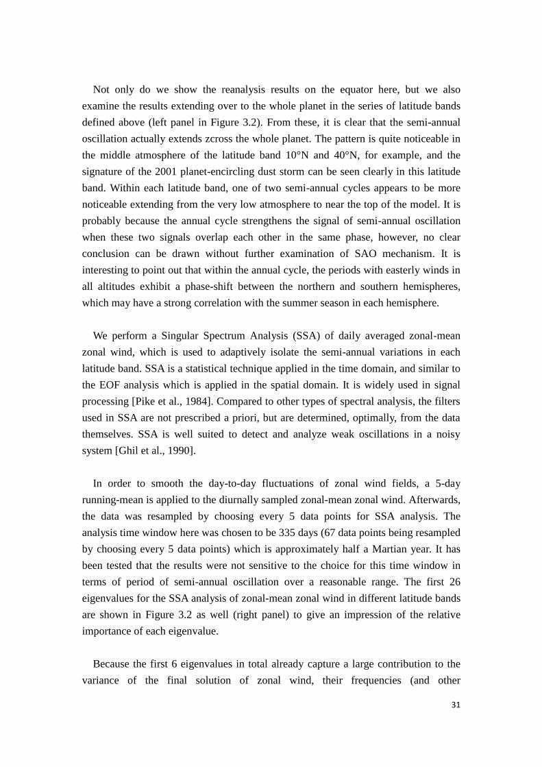
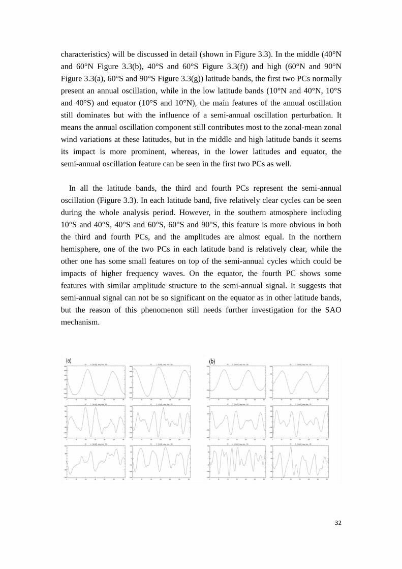
Figure 3.3. The PCs of the first 6 eigenvalues in different latitude bands. In each figure the

upper two is the first pair of PCs, the middle two is the second pair and the lower two is the

third pair of PCs, (a) for 60°N and 90°N, (b) for 40°N and 60°N, (c) for 10°N and 40°N, (d)

for 10°S and 10°N, (e) for 10°S and 40°S, (f) for 40°S and 60°S, (g) for 60°S and 90°S.

34

The fifth and sixth PCs in high latitudes of the northern hemisphere (60°N and

90°N) also indicate some semi-annual oscillation signal. However, in most of the

other latitude bands, the fifth and sixth PCs appear to represent the high-frequency

patterns, especially in the southern hemisphere. Besides, it is interesting to mention

that these two PCs in the low latitudes of the northern hemisphere (10°N and 40°N)

and equator (10°S and 10°N) shows some abrupt changes of amplitude during the

2001 planet-encircling dust storm (MY 25). The further relationship among these two

components, corresponding to an increase of actual zonal wind and perhaps

contributing further to trigger the 2001 planet-encircling dust storm could be an

interesting topic to investigate further in future.

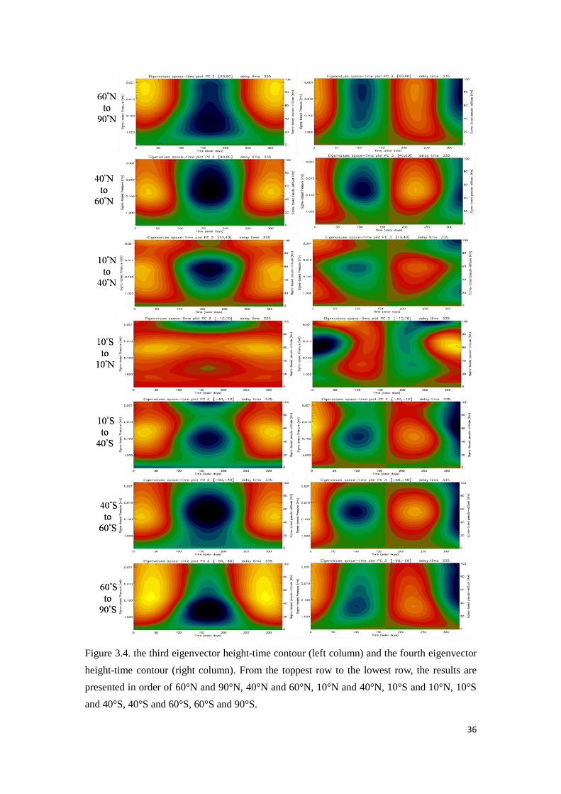
Within the chosen analysis time window (335 days) for SSA analysis, height-time

plots present the distribution of semi-annual oscillation activity in terms of height and

time (Figure 3.4). It is obvious that in each latitude band a slight phase difference can

be seen between the third eigenvector and fourth eigenvector, i.e. the signals

represented by the third eigenvector almost start from the highest positive value then

change to the lowest negative value, and back to the positive value again, while the

signals represented by the fourth eigenvector except at the equator start from a

positive value but change quickly to low values, and go through a full half-cycle to

negative values again. It indicates that the phase of the fourth eigenvector can be near

45° ahead of the phase of the third eigenvector, and probably the oscillation cycle of

fourth eigenvector is slightly shorter than for the third eigenvector. It is noticeable that

the clear semi-annual oscillation signals can penetrate all the way to the upper

atmosphere from the lower atmosphere in each latitude band, and the maximum in

amplitude of the semi-annual oscillation happens in the middle atmosphere. However,

this phenomenon is more significant in the middle and high latitude bands of the

northern hemisphere (60°N and 90°N, 40°N and 60°N) and the southern hemisphere

(10°S and 40°S, 40°S and 60°S, 60°S and 90°S)

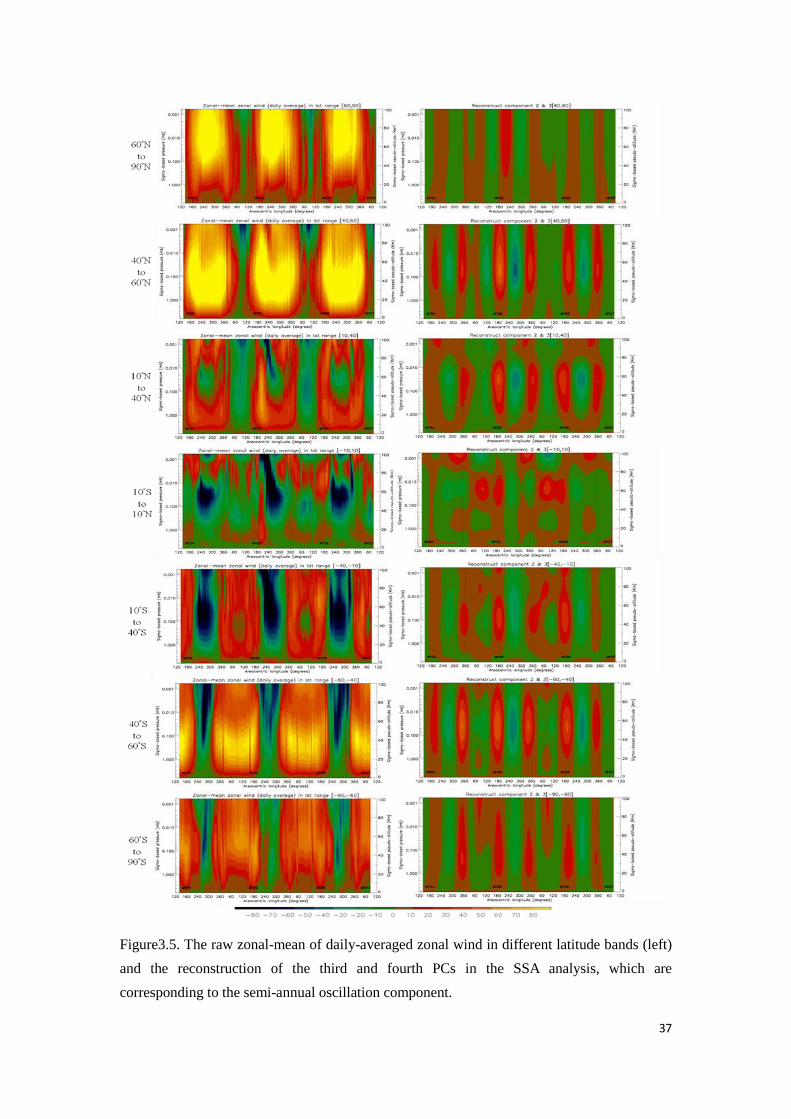
The third and fourth PCs in the SSA analysis are also reconstructed to demonstrate

the semi-annual oscillation components in terms of daily-averaged zonal-mean zonal

wind in different latitude bands (see Figure 3.5). Between 10°S and 10°N, the pattern

represented by these two PCs in reconstruction is relatively complicated, perhaps

because dynamical conditions at the equator can be strongly affected by plenty of

factors. But the semi-annual oscillation can be observed extremely clearly in the

middle atmosphere (altitude 40km ~ 80km) even in the raw zonal-mean of

daily-averaged zonal wind at the equator (10°S and 10°N) and the low latitude bands

35

regardless of hemisphere (10°N and 40°N , 10°S and 40°S). Extending to the polar

regions, the semi-annual oscillation becomes more significant, but the overall

amplitude reaches its maximum in the middle latitude bands (40°N and 60°N, 40°S

and 60°S) in both hemispheres. However, unlike at the equator and at low latitudes,

one of two semi-annual oscillations in the middle latitude bands (40°N and 60°N,

40°S and 60°S) and the high latitude bands (60°N and 90°N, 60°S and 90°S) are not

found in the corresponding raw zonal-mean of daily-averaged zonal wind.

Furthermore, it is noticeable that within each latitude band, a maximum of

semi-annual oscillation components seems to appear during the 2001

planet-encircling dust storm.

36

Figure 3.4. the third eigenvector height-time contour (left column) and the fourth eigenvector

height-time contour (right column). From the toppest row to the lowest row, the results are

presented in order of 60°N and 90°N, 40°N and 60°N, 10°N and 40°N, 10°S and 10°N, 10°S

and 40°S, 40°S and 60°S, 60°S and 90°S.

37

Figure3.5. The raw zonal-mean of daily-averaged zonal wind in different latitude bands (left)

and the reconstruction of the third and fourth PCs in the SSA analysis, which are

corresponding to the semi-annual oscillation component.

38

Chapter 4 2-D Data Assimilation of Column Dust Opacity

with Dust Transport

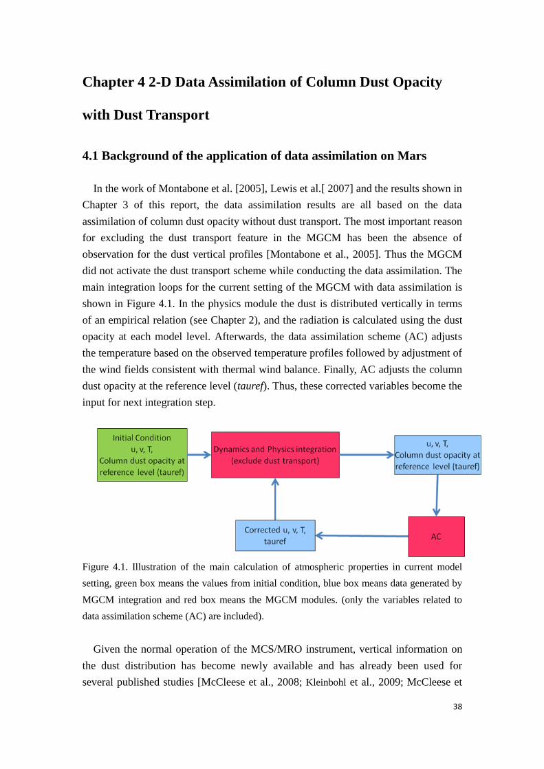
4.1 Background of the application of data assimilation on Mars

In the work of Montabone et al. [2005], Lewis et al.[ 2007] and the results shown in

Chapter 3 of this report, the data assimilation results are all based on the data

assimilation of column dust opacity without dust transport. The most important reason

for excluding the dust transport feature in the MGCM has been the absence of

observation for the dust vertical profiles [Montabone et al., 2005]. Thus the MGCM

did not activate the dust transport scheme while conducting the data assimilation. The

main integration loops for the current setting of the MGCM with data assimilation is

shown in Figure 4.1. In the physics module the dust is distributed vertically in terms

of an empirical relation (see Chapter 2), and the radiation is calculated using the dust

opacity at each model level. Afterwards, the data assimilation scheme (AC) adjusts

the temperature based on the observed temperature profiles followed by adjustment of

the wind fields consistent with thermal wind balance. Finally, AC adjusts the column

dust opacity at the reference level (tauref). Thus, these corrected variables become the

input for next integration step.

Figure 4.1. Illustration of the main calculation of atmospheric properties in current model

setting, green box means the values from initial condition, blue box means data generated by

MGCM integration and red box means the MGCM modules. (only the variables related to

data assimilation scheme (AC) are included).

Given the normal operation of the MCS/MRO instrument, vertical information on

the dust distribution has become newly available and has already been used for

several published studies [McCleese et al., 2008; Kleinbohl et al., 2009; McCleese et

39

al., 2010]. As a result, it also provides the possibility of conducting 3-D dust

assimilation with dust transport feature activated in the MGCM. Once this is

implemented in the MGCM, it can make full use of the retrievals of dust profiles to

obtain a more detailed understanding of the Martian atmosphere both in the weather

aspects and the climatology. This chapter will present the recent progress of the first

attempt to implement this more advanced data assimilation scheme by combining the

2-D dust data assimilation and dust transport scheme including dust lifting

mechanisms (hereafter, dust transport scheme). Full 3-D dust assimilation will remain

the ultimate future objective.

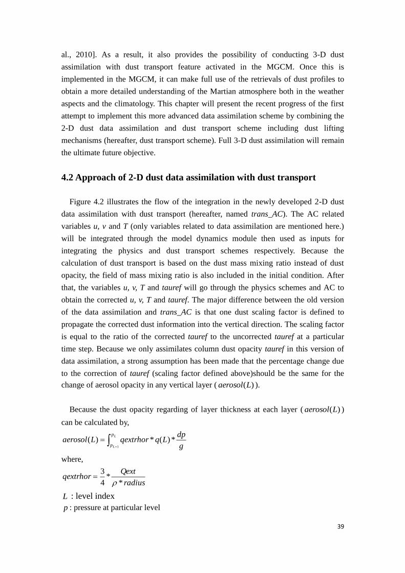
4.2 Approach of 2-D dust data assimilation with dust transport

Figure 4.2 illustrates the flow of the integration in the newly developed 2-D dust

data assimilation with dust transport (hereafter, named trans_AC). The AC related

variables u, v and T (only variables related to data assimilation are mentioned here.)

will be integrated through the model dynamics module then used as inputs for

integrating the physics and dust transport schemes respectively. Because the

calculation of dust transport is based on the dust mass mixing ratio instead of dust

opacity, the field of mass mixing ratio is also included in the initial condition. After

that, the variables u, v, T and tauref will go through the physics schemes and AC to

obtain the corrected u, v, T and tauref. The major difference between the old version

of the data assimilation and trans_AC is that one dust scaling factor is defined to

propagate the corrected dust information into the vertical direction. The scaling factor

is equal to the ratio of the corrected tauref to the uncorrected tauref at a particular

time step. Because we only assimilates column dust opacity tauref in this version of

data assimilation, a strong assumption has been made that the percentage change due

to the correction of tauref (scaling factor defined above)should be the same for the

change of aerosol opacity in any vertical layer ( )(Laerosol ).

Because the dust opacity regarding of layer thickness at each layer ( )(Laerosol )

can be calculated by,

L

L

p

p g

dpLqqextrhorLaerosol

1

*)(*)(

where,

radius

Qextqextrhor

**

4

3

L : level index

p : pressure at particular level

40

q : dust mass mixing ratio

g : gravitational acceleration on Mars

Qext : extinction coefficient

: dust density

radius : stand for radius of dust particle

Figure 4.2. Illustration of the main calculation of atmospheric properties in the newly

developed scheme, green box means the values from initial condition, blue box means data

generated by MGCM integration and red box means the MGCM modules. (only the variables

related to data assimilation scheme (AC) are included)

Meanwhile, the column dust opacity can be obtained by simply summing up

)(Laerosol in the vertical direction. At a particular integration time step, the

extinction coefficient and layer thickness should be constant for particular model grid

at certain layer. As a result, the scaling factor can be applied directly to multiply dust

mass mixing ratio q to perform the correction.

4.3 Preliminary results

The preliminary results present in this chapter are for only 30 days simulation,

starting from Martian day 331 to day 361 in MY 24. They all start from the same

initial condition, although the initial condition may not be perfect (e.g. only 60 days

spin-up time). In each figure, the upper panel is from the free running MGCM with

dust transport scheme activated (hereafter, trans), middle panel is from the existing

data assimilation without dust transport (hereafter, ACM), while the bottom one is for

41

AC with dust transport, denoted as trans_AC.

In order to easily understand the results produced by this new approach, only one

dust particle size bin is chosen for this preliminary study of MGCM column dust data

assimilation with dust transport, although multi-size dust transport and the capability

of predicting the distribution of dust particle sizes is also included in the MGCM. The

possibility of conducting data assimilation with multi-size dust transport could be

investigated in future work beyond this project. In addition, other dust transport

related mechanisms (radiatively active dust, dust lifting by wind stress, dust lifting by

dust devil and sedimentation) remain functional.

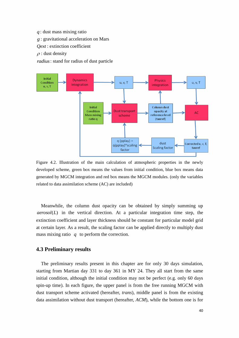
Figure 4.3. column dust opacity simulated by MGCM, in each figure, upper panel is for trans

scenario, middle panel is for ACM scenario and lower panel is for trans_AC scenario (new

approach), (a) the first two-hour simulation, (b) simulation results after 5 days from initial, (c)

simulation results after 15 days from initial, (d) simulation results after 25 days from initial.

The simulation results for three scenarios are shown in Figure 4.3. The results are

output every two hours during the simulation, and after the first two hours (Figure

4.3a), the nearly similar patterns (high column dust opacity on Hellas) coming from

initial conditions can still be observed at this early simulation time. After 5 days

integration, the dust starts to accumulate on the equator, and at low and middle

42

latitudes in the trans scenario (upper panel in Figure 4.3b). It is noticeable that in the

trans scenario more dust spreads into the northern hemisphere compared to the

southern hemisphere, and three regions of high column dust opacity develop in the

northern hemisphere. For the ACM (middle panel in Figure 4.3b) and trans_AC (lower

panel in Figure 4.3b) cases, the patterns for the dust distribution are quite similar to

each other, except that in high southern latitudes, a dust transport path can be

observed between two areas of high column dust opacity. 15 days from initialization

(Figure 4.3c), the dust continues to accumulate in the northern hemisphere in trans

(upper panel in figure 4.3c), and the column dust opacity is higher in both high value

areas of the southern hemisphere in trans_AC than those in ACM (location around

(-45°S, -45° in longitude), (-45°S, 60° in longitude)). Moreover, areas with column

dust opacity higher than 0.8 cover most of the south polar area in trans_AC. In the day

25 of trans, plenty of dust have formed a band with high column dust opacity in the

middle latitudes of northern hemisphere (30°N). The main difference between ACM

and trans_AC is the higher column dust opacity in the dust-rich area of southern

hemisphere ((-45°S, 60° in longitude)). Overall, the results of ACM and trans_AC are

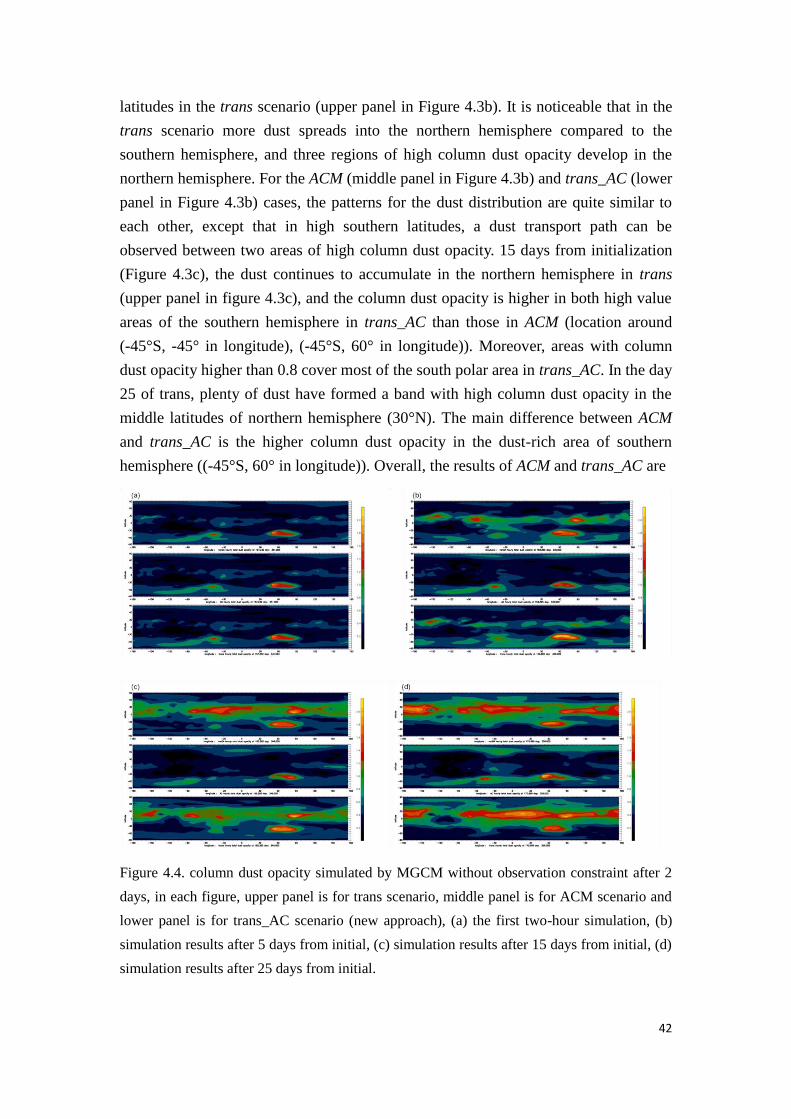
Figure 4.4. column dust opacity simulated by MGCM without observation constraint after 2

days, in each figure, upper panel is for trans scenario, middle panel is for ACM scenario and

lower panel is for trans_AC scenario (new approach), (a) the first two-hour simulation, (b)

simulation results after 5 days from initial, (c) simulation results after 15 days from initial, (d)

simulation results after 25 days from initial.

43

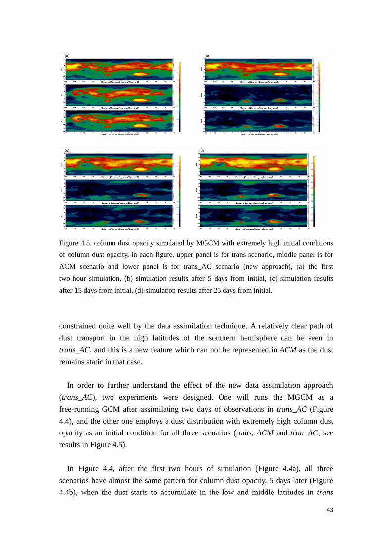
Figure 4.5. column dust opacity simulated by MGCM with extremely high initial conditions

of column dust opacity, in each figure, upper panel is for trans scenario, middle panel is for

ACM scenario and lower panel is for trans_AC scenario (new approach), (a) the first

two-hour simulation, (b) simulation results after 5 days from initial, (c) simulation results

after 15 days from initial, (d) simulation results after 25 days from initial.

constrained quite well by the data assimilation technique. A relatively clear path of

dust transport in the high latitudes of the southern hemisphere can be seen in

trans_AC, and this is a new feature which can not be represented in ACM as the dust

remains static in that case.

In order to further understand the effect of the new data assimilation approach

(trans_AC), two experiments were designed. One will runs the MGCM as a

free-running GCM after assimilating two days of observations in trans_AC (Figure

4.4), and the other one employs a dust distribution with extremely high column dust

opacity as an initial condition for all three scenarios (trans, ACM and tran_AC; see

results in Figure 4.5).

In Figure 4.4, after the first two hours of simulation (Figure 4.4a), all three

scenarios have almost the same pattern for column dust opacity. 5 days later (Figure

4.4b), when the dust starts to accumulate in the low and middle latitudes in trans

44

(upper panel in Figure 4.4b), some dusts also starts to accumulate in low latitudes in

trans_AC (lower panel in Figure 4.4b), and for the areas with high column dust

opacity of southern hemisphere, the one near (-45°S, -45° in longitude) appears to

dissipate, and the one near (-45°S, 60° in longitude) has highest value than those in

the other scenarios. 15 days from initial (Figure 4.4c), trans_AC has formed similar

pattern of column dust opacity to that in trans, but with smaller coverage of column

dust opacity higher than 1.2. In day 25 (Figure 4.4d), the values of column dust

opacity in northern hemisphere looks indicate more dusts accumulate in trans_AC

than that in trans.

Figure 4.5 shows the experiment with an extremely high initial condition of column

dust opacity. Extremely high column dust opacity can still be seen in Figure 4.5a after

the first two hours from starting the simulation. However, in day 5 (Figure 4.5), the

redundant dusts in the ACM (middle panel in Figure 4.5b) and trans_AC (lower panel

in Figure 4.5b) have been “removed” by the data assimilation scheme, and the

patterns became similar to the corresponding plots in Figure 4.3. Evolving with time,

the high column dust opacity in the trans simulation indicates the redundant dust can

not be “removed” at the finish of whole 30-day simulation by the dust sedimentation

scheme in MGCM, but the data assimilation scenarios (ACM and trans_AC)

eventually converge back to the results shown in Figure 4.3.

45

Chapter 5 Conclusions and Future Plans

5.1 Conclusions

This report presents the works which has been done in my first year enrolled in the

DPhil program in Atmospheric, Oceanic and Planetary Physics (AOPP) of the

University of Oxford. A Martian General Circulation Model (MGCM), developed

mainly in UK (University of Oxford and The Open University) with joint efforts of

Laboratoire de Météorologie Dynamique (LMD; Paris, France) and Instituto de

Astrofisica de Andalucia (Granada, Spain), is employed in this DPhil project to make

use of the newly available vertically resolved dust opacity data from MCS. In terms of

that particular purpose, a more advanced data assimilation technique has to be

developed. The current data assimilation scheme in MGCM only assimilates the

temperature profiles and column dust opacity at a reference level (tauref), and the dust

would not be transported in the light of model predicted variables. In terms of

technical aspects, our aim is to develop a new data assimilation scheme which is able

to assimilate the profiles of dust opacity to correct the dust fields predicted by the

MGCM dust transport scheme. Based on this new data assimilation technique and

available observations, a complete and dynamically self-consistent reconstruction of

the entire global circulation will be made. Such a record will then be used for a

series of diagnostic studies to characterize the detailed climatology and synoptic

meteorology of Mars over seasonal and interannual timescales. This can include

detailed case studies of events such as the formation of cyclonic weather systems and

initiation of regional dust storms.

The work of analyzing the semi-annual oscillation from the assimilated results

produced by Montabone et al. [2005] has been presented not only in the Chapter 3 of

this report, but also in the Fourth International workshop on the Mars Atmosphere:

modeling and observations held in Paris, France in February of 2011. We analyzed the

raw zonal-mean of daily-averaged zonal wind to obtain survey of the semi-annual

oscillation in the Martian atmosphere and its structure in the different latitude bands

(see Figure 3.2). Afterwards, the details of the Martian semi-annual oscillation were

unveiled on the basis of Singular Spectrum Analysis (SSA). The second largest pair of

Principal Components (PCs) represents the semi-annual oscillation, and their

corresponding eigenvectors show that a coherent semi-annual signal can be observed

in most altitudes outside the Planetary Boundary Layer (PBL), especially outside the

equator. The reconstructions of the third and fourth PCs indicate the semi-annual

46

oscillation can be amplified by the annual oscillation signal. On extending the view to

the polar regions, the semi-annual oscillation becomes more significant, but the

overall amplitude reaches its maximum in the middle latitude bands (40°N and 60°N,

40°S and 60°S) in both hemispheres. This phenomenon can not be seen clearly in the

raw zonal-mean of daily-averaged zonal wind, since the amplitude of annual

oscillation is too strong and obscures this feature. However, in the low latitudes of

northern hemisphere (10°N and 40°N) and equator (10°S and 10°N), the cause of the

interesting abrupt changes of fifth PC amplitude during the 2001 planet-encircling

dust storm (MY 25) is still under investigation.

The progress of developing data assimilation scheme with dust transport was

addressed in Chapter 4 of this report. Our first attempt was to assimilate the observed

tauref to further correct the predicted dust mixing ratio based on the assumption that

the percentage change due to the correction of tauref should be the same in any

vertical layer. This approach actually propagates the 2-D dust information into the

vertical on the basis of an assumption that the scaling factor defined above is the same

for particular model grid at particular time step in different layers. The preliminary

results seem to be reasonable and encouraging. While showing the dust transport path

predicted by the dust transport scheme, the new data assimilation approach presented

in this report can still remove excess dust when required by the observations, making

the final simulation converge to the simulation produced by the old assimilation

scheme. Certainly, further investigations still need to be done to validate this method,

and to provide the useful experience to the assimilation of dust opacity profiles with

dust transport.

5.2 Future Work

For the study of the Martian semi-annual oscillation, the next step is to investigate

the possible trigger and related effect of abrupt changes of fifth PC in the low latitude

of northern hemisphere (10°N and 40°N) and equator (10°S and 10°N). So far, the

triggers of dust events especially the global dust storms on Mars have not yet been

found out. It is interesting that this abrupt change of fifth PC from the SSA of

zonal-mean zonal wind happens more or less at the time of the start of 2001

planet-encircling dust storm (MY 25). Thus, to question if this abrupt change is a

side-effect of the global dust storm or if this is the trigger of the global dust storm can

be an interesting topic to look into, and probably lead this study to completion in

January of year 2012. In the coming three months, the possible correlation between

the phase change of the semi-diurnal tide and the abrupt amplitude change of

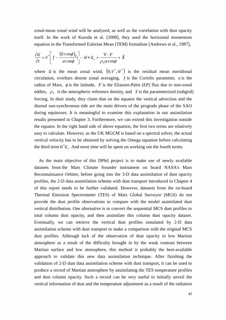
47

zonal-mean zonal wind will be analyzed, as well as the correlation with dust opacity

itself. In the work of Kuroda et al. [2008], they used the horizontal momentum

equation in the Transformed Eulerian Mean (TEM) formalism [Andrews et al., 1987],

X

a

Fuw

a

ufv

t

uz

coscos

cos

0

*

where u is the mean zonal wind, ** ,,0 wv is the residual mean meridional

circulation, overbars denote zonal averaging, f is the Coriolis parameter, a is the

radius of Mars, is the latitude, F is the Eliassen-Palm (EP) flux due to non-zonal

eddies, 0 is the atmospheric reference density, and X is the parameterized (subgrid)

forcing. In their study, they claim that on the equator the vertical advection and the

diurnal sun-synchronous tide are the main drivers of the prograde phase of the SAO

during equinoxes. It is meaningful to examine this explanation in our assimilation

results presented in Chapter 3. Furthermore, we can extend this investigation outside

the equator. In the right hand side of above equation, the first two terms are relatively

easy to calculate. However, as the UK MGCM is based on a spectral solver, the actual

vertical velocity has to be obtained by solving the Omega equation before calculating

the third term zuw * . And most time will be spent on working out the fourth terms.

As the main objective of this DPhil project is to make use of newly available

datasets from the Mars Climate Sounder instrument on board NASA's Mars

Reconnaissance Orbiter, before going into the 3-D data assimilation of dust opacity

profiles, the 2-D data assimilation scheme with dust transport introduced in Chapter 4

of this report needs to be further validated. However, datasets from the on-board

Thermal Emission Spectrometer (TES) of Mars Global Surveyor (MGS) do not

provide the dust profile observations to compare with the model assimilated dust

vertical distribution. One alternative is to convert the sequential MCS dust profiles to

total column dust opacity, and then assimilate this column dust opacity dataset.

Eventually, we can retrieve the vertical dust profiles simulated by 2-D data

assimilation scheme with dust transport to make a comparison with the original MCS

dust profiles. Although lack of the observation of dust opacity in low Martian

atmosphere as a result of the difficulty brought in by the weak contrast between

Martian surface and low atmosphere, this method is probably the best-available

approach to validate this new data assimilation technique. After finishing the

validation of 2-D dust data assimilation scheme with dust transport, it can be used to

produce a record of Martian atmosphere by assimilating the TES temperature profiles

and dust column opacity. Such a record can be very useful to initially unveil the

vertical information of dust and the temperature adjustment as a result of the radiation

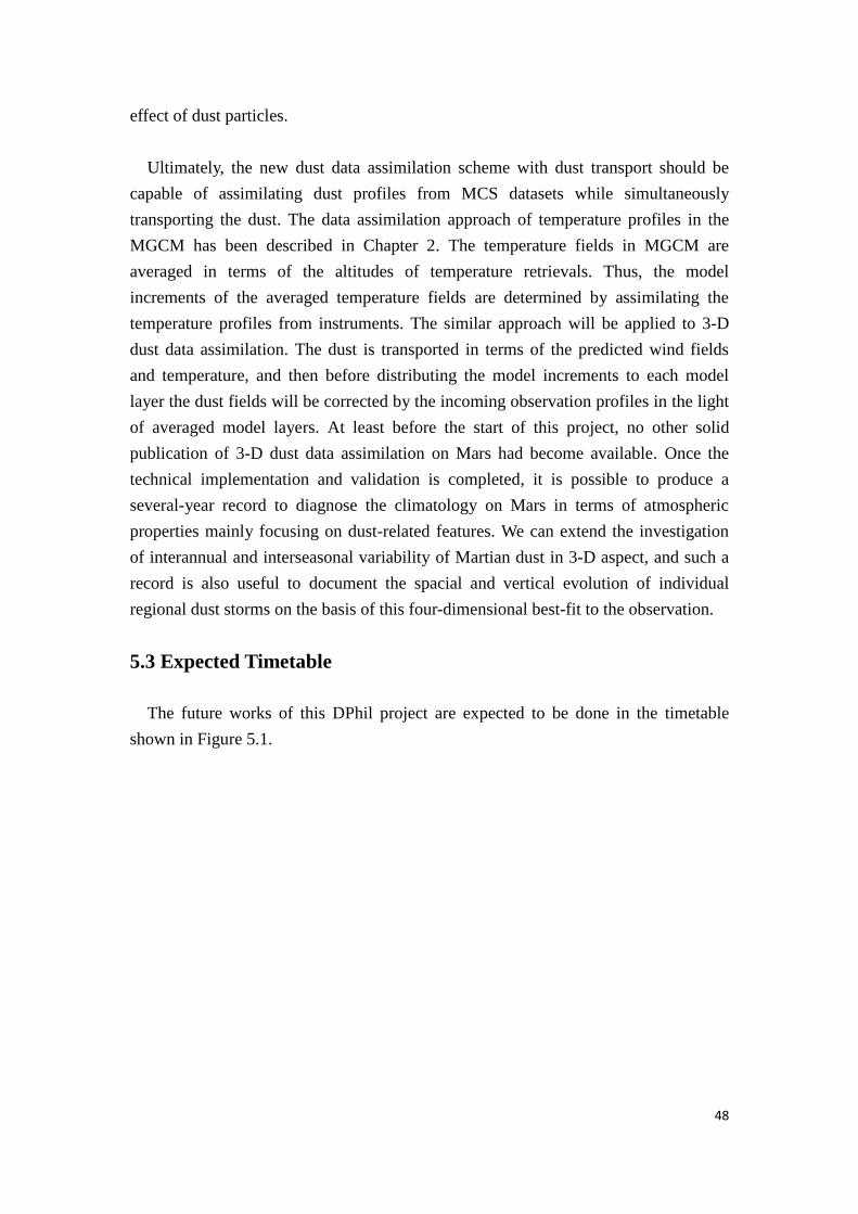
48

effect of dust particles.

Ultimately, the new dust data assimilation scheme with dust transport should be

capable of assimilating dust profiles from MCS datasets while simultaneously

transporting the dust. The data assimilation approach of temperature profiles in the

MGCM has been described in Chapter 2. The temperature fields in MGCM are

averaged in terms of the altitudes of temperature retrievals. Thus, the model

increments of the averaged temperature fields are determined by assimilating the

temperature profiles from instruments. The similar approach will be applied to 3-D

dust data assimilation. The dust is transported in terms of the predicted wind fields

and temperature, and then before distributing the model increments to each model

layer the dust fields will be corrected by the incoming observation profiles in the light

of averaged model layers. At least before the start of this project, no other solid

publication of 3-D dust data assimilation on Mars had become available. Once the

technical implementation and validation is completed, it is possible to produce a

several-year record to diagnose the climatology on Mars in terms of atmospheric

properties mainly focusing on dust-related features. We can extend the investigation

of interannual and interseasonal variability of Martian dust in 3-D aspect, and such a

record is also useful to document the spacial and vertical evolution of individual

regional dust storms on the basis of this four-dimensional best-fit to the observation.

5.3 Expected Timetable

The future works of this DPhil project are expected to be done in the timetable

shown in Figure 5.1.

49

Figure 5.1. Expected timetable for the future works of DPhil project.

50

Bibliography

Basu, S., M. I. Richardson and R. J. Wilson (2004), Simulation fo the Martian dust cycle with

the GFDL Mars GCM, J. Gerphys., Res. 109(E11006), doi: 10.1029/2004JE002243.

Benson J. L., D. M. Kass and MCS Team (2011), Mars Climate Sounder observations of ice

and dust layering in the Martian atmosphere, Fourth International Workshop on Mars

Atmosphere Modeling and Obsevations, Paris, France, Feb. 2011.

Cantor, B. A., P. B. James, M. Caplinger, and M. J. Wolff, Martian dust storms: 1999 Mars

Orbiter Camera observations. J. Geophys. Res. 106, 23, 653-23,687, 2001.

Collins., M., S. R. Lewis, P. L. Read and F. Hourdin (1996), Baroclinic wave transitions in the

Martian atmosphere, Icarus, 120, 344-357.

Conrath, B. J. (1975), Thermal structure of the Martian atmosphere during the dissipation of

dust storm of 1971, Icarus, 24, 36-46, 1975.

Conrath, B. J., J. C. Pearl, M. D. Smith, W. C. Maguire, S. Dason, M. S. Kaelbere and P .R.

Christensen (2000), Mars Global Surveyor Thermal Emission Spectrometer (TES)

observations: atmospheric temperatures during aerobraking and science phasing, J. Geophys.

Res. 105 ,9509-9520.

Euler, E. A., S. D. Jolly and H. H. „Lad‟ Curtis (2001), The failures of the Mars Climate

Orbiter and Mars Polar Lander: a perspective from the people involved, 24th annual AAS

guidance and control conference, January 31-February 4, 2001, Brechenridge, Colorado,

USA.

Fenton, L. K., and M. I. Richardson (2001), Martian surface winds: Insensitivity to orbital

changes and implications for aeolian processes, J. Geophys. Res., 106, 32,885– 32,902

Forget, F., F. Hourdin, R. Fournier, C. Hourdin, O. Talagrand, M. Collins, S. R. Lewis, P. L.

Read and J.-P. Huot (1999), Improved general circulation models of the martian atmosphere

from the surface to above 80 km, J. Gerphys., Res. 104 (E10), 24155-24176.

Garcia, R. R., T. J. Dunkerton, R. S. Lieberman and R. A. Vincent (1997), Climatology of the

semiannual oscillation of the tropical middle atmosphere, J. Gerphys., Res., 102,

51

26019-26032.

Ghil, M. and K. Mo (1990), Intraseasonal oscillations in the global atmosphere. Part II:

Southern Hemisphere, J. Atmos. Sci., 48(5),780-790.

Hamilton, K. (1995), Interannual variability in the northern hemisphere winter middle

atmosphere in control and perturbed experiments with the GFDL SKYHI general circulation

model, J. Atmos. Sci., 52, 44–66.

Hoskins, B. J. and A. J. Simmons (1975), A multi-layer spectral model and the semi-implicit

method, Q. J. R. Meteorol. Soc., 101, 637-655.

Hourdin, F., F. Forget, and O. Talagrand (1995), The sensitivity of the Martian surface

pressure and atmospheric mass budget to various parameters: A comparison between

numerical simulations and Viking observations, J. Geophys. Res., 100(E3), 5501–5523,

doi:10.1029/94JE03079.

Kahre, M. A. and R. M. Haberle (2010), Mars CO2 cycle: Effects of airborne dust and polar

cap ice emissivity, Icarus, 201, 648-653.

Kuroda, T., A. S. Medvedev, P. Hartogh and M. Takahashi (2008), Semiannual oscillations in

the atmosphere of Mars, Geophys. Res. Lett., 35, L23202, doi:10.1029/2008GL036061.

Lee, C., et al. (2009), Thermal tides in the Martian middle atmosphere as seen by the Mars

Climate Sounder, J. Geophys. Res., 114, E03005, doi:10.1029/2008JE003285.

Lewis, S. R. and P. R. Barker (2005), Atmospheric tides in a Mars general circulation model

with data assimilation, Adv. Space Res. 36(11), 2162-2168.

Lewis, S. R., P. L. Read, B. J. Conrath, J. C. Pearl and M. D. Smith (2007), Assimilation of

thermal emission spectrometer atmospheric data during the Mars Global Surveyor

aerobraking period, Icarus 192, 327-347.

Lorenc, A. C., R. S. Bell and B. Macpherson (1991), The meteorological office analysis

correction data assimilation scheme, Q. J. R. Meteor. Soc., 117, 59-89.

Mellor, G. L. and T. Yamada (1982), Development of a turbulence closure model for

geophysical fluid problems, Rev. of Geophys., 20, 851-875.

52

McCleese, D. J., et al. (2008), Intense polar temperature inversion in the middle atmosphere

on Mars, Nat. Geosci., 1, 745–749, doi:10.1038/ngeo332.

McCleese, D. J., et al. (2010), Structure and dynamics of the Martian lower and middle

atmosphere as observed by the Mars Climate Sounder: Seasonal variations in zonal mean

temperature, dust, and water ice aerosols, J. Geophys. Res., 115, E12016,

doi:10.1029/2010JE003677.

Montabone, L., S. R. Lewis and P. L. Read (2005), Interannual variability of martian dust

storm in assimilation of several years of Mars Global Surveyor observations, Adv. Space Res.

36 (11) , 2146-2155.

Montabone, L., S. R. Lewis, P. L. Read and D. P. Hinson (2006a), Validation of martian

meteorological data assimilation for MGS/TES using radio occultation measurements, Icarus

185 (1), 113-132.

Montabone, L., S. R. Lewis and P. Withers (2006b), Reconstructing the weather on Mars at

the time of the MERs and Beagle 2 landings, Geophys. Res. Lett., 33, L19202.

Montabone, L., E. Millour and F. Forget (2010), WP 1.6 deliverable : Report on the analysis

of available atmospheric observations at Exomars‟ phase B2X landing site, Laboratoire de

M´et´eorologie Dynamique, Universit´e “Pierre et Marie Curie”, Paris, France, March 31

2010.

Murphy, J. R., J. B. Pollack, R. M. Haberle, C. B. Leovy, O. B. Toon, and J.

Schaeffer (1995), Three-dimensional numerical simulation of Martian global dust storms, J.

Geophys. Res., 100(E12), 26,357–26,376, doi:10.1029/95JE02984.

Newman, C. E., S. R. Lewis, P. L. Read and F. Forget (2002), Modeling the Martian dust

cycle 1. Representations of dust transport processes, J. Gerphys., Res., 107(E12), 5123,

doi:10.1029/2002JE001910, 2002.

Newman , C. E., S. R. Lewis, P. L. Read and F. Forget (2002), Modeling the Martian dust

cycle, 2, Multiannual radiatively active dust transport simulations, J. Gerphys., Res.,107(E12),

5124, doi:10.1029/2002JE001920, 2002.

Pike, E. R., J. G. McWhirter, M. Bertero and C. deMol, (1984), Generalized information

53

theory for inverse problems in signal processing, IEEE Proc., 131, 660-667.

Read, P. L. and S. R. Lewis (2004), The Martian Climate Revisited: Atmosphere and

Environment of a desert planet, Praxis Publishing Ltd, Chichester, UK, 2004, printed in

Germany.

Reed, J. R. (1966), Zonal wind behavior in the equatorial stratosphere and lower mesosphere,

J. Gerphys., Res., 71, 4223-4233

Rennó, N. O., A. A. Nash, J. Lunine and J. Murphy (2000), Martian and terrestrial dust devils:

test of a scaling theory using Pathfinder data, J. Gerphys., Res.,105(E1), 1859-1865.

Rogberg, P., P. L. Read, S. R. Lewis and L. Montabone (2010), Assessing atmospheric

predictability on Mars using numerical weather prediction and data assimilation, Q. J. R.

Meteorol. Soc., 136, 1614-1635.

Schofield, J. T., D. M. Kass, A. Kleinböhl, D. J. McCleese, M. A. Allen, M. C. Foote, M.

Jeganathan, F. Forget, A. Spiga, O. Talagrand, F. Lefèvre, A. Määttänen, T. Fouchet, N.

Bowles, S. B. Calcutt, P. G. J. Irwin, P. L. Read, S. R. Lewis, J. R. Barnes, S. W. Bougher, R.

M. Haberle (2011), The Exomars Climate Sounder (EMCS) investigation, Fourth

International Workshop on Mars Atmosphere Modeling and Obsevations, Paris, France, Feb.

2011.

Smith, M. D. (2004), Interannual variability in TES atmospheric observations of Mars during

1999-2003, Icarus, 167, 148-165.

Sutton, J. L., C. B. Leovy and J. E. Tillman (1978), Diurnal variations of the Martian surface

layer meteorological parameters during first 45 sols at two Viking lander sites, J. Atmos.

Sci.,35, 2346-2355.

Toon, O. B., J. B. Pollack and C. Sagan, Physical properties of the particles composing the

Martian dust storm, Icarus, 30, 663-696, 1977.

Wilson, R. J., and K. Hamilton (1996), Comprehensive model simulations of thermal tides in

the Martian atmosphere, J. Atmos. Sci., 53, 1290–1326.

Wilson, R. J., S. R. Lewis, L. Montabone and M. D. Smith (2008), Influence of water ice

clouds on Martian tropical atmospheric temperatures, Geophys, Res. Lett., 35, L07202.