The Classical Theory of Inflation -...

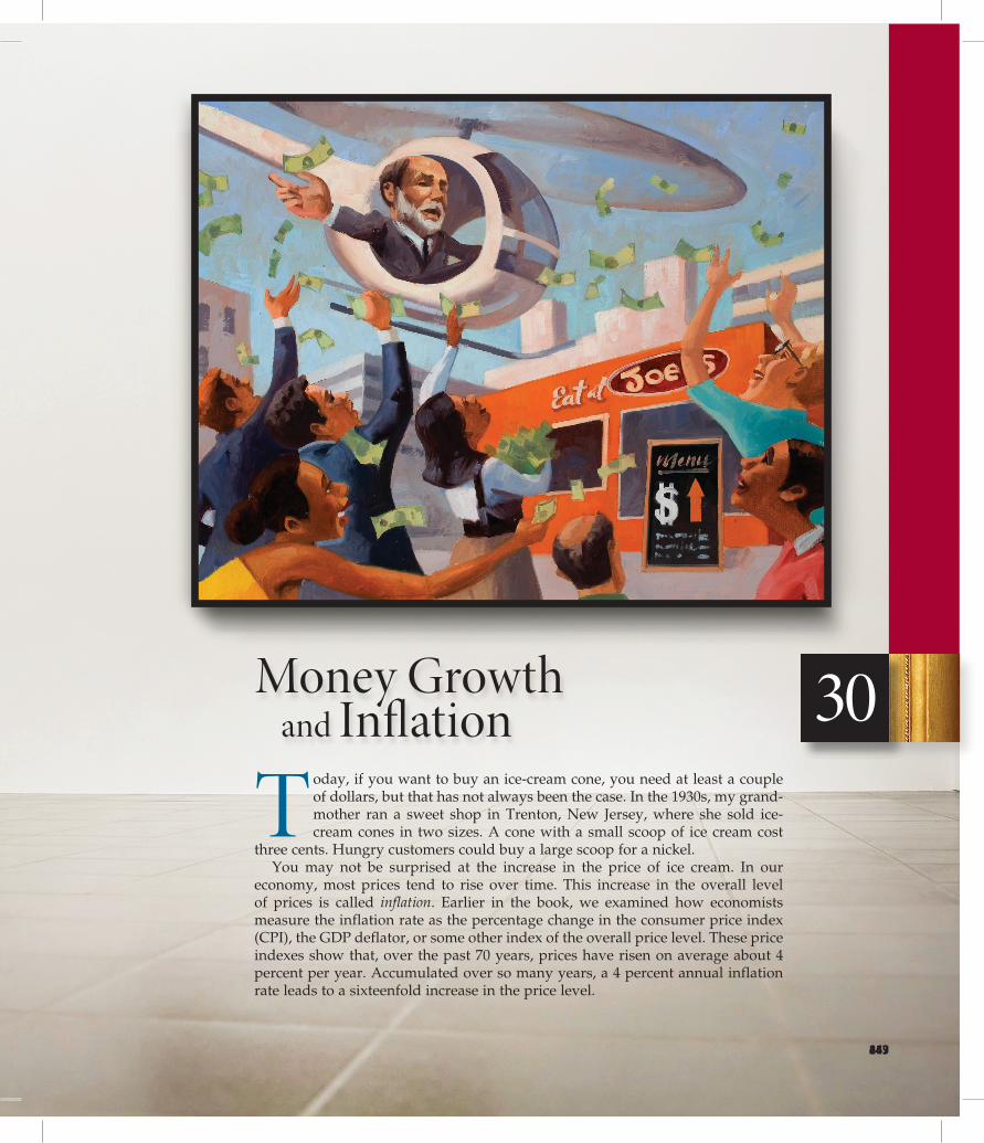
T oday, if you want to buy an ice-cream cone, you need at least a couple of dollars, but that has not always been the case. In the 1930s, my grand-mother ran a sweet shop in Trenton, New Jersey, where she sold ice-cream cones in two sizes. A cone with a small scoop of ice cream cost

three cents. Hungry customers could buy a large scoop for a nickel.You may not be surprised at the increase in the price of ice cream. In our

econo my, most prices tend to rise over time. This increase in the overall level of prices is called inflation. Earlier in the book, we examined how economists measure the inflation rate as the percentage change in the consumer price index (CPI), the GDP deflator, or some other index of the overall price level. These price indexes show that, over the past 70 years, prices have risen on average about 4 percent per year. Accumulated over so many years, a 4 percent annual inflation rate leads to a sixteenfold increase in the price level.

Money Growth and Inflation

243

12

347

17

459

22

643

30

Inflation may seem natural and inevitable to a person who grew up in the United States during recent decades, but in fact, it is not inevitable at all. There were long periods in the 19th century during which most prices fell—a phenome-non called deflation. The average level of prices in the U.S. economy was 23 percent lower in 1896 than in 1880, and this deflation was a major issue in the presidential election of 1896. Farmers, who had accumulated large debts, suffered when the fall in crop prices reduced their incomes and thus their ability to pay off their debts. They advocated government policies to reverse the deflation.

Although inflation has been the norm in more recent history, there has been substantial variation in the rate at which prices rise. During the 1990s, prices rose at an average rate of about 2 percent per year. By contrast, in the 1970s, prices rose by 7 percent per year, which meant a doubling of the price level over the decade. The public often views such high rates of inflation as a major economic problem. In fact, when President Jimmy Carter ran for reelection in 1980, challenger Ronald Reagan pointed to high inflation as one of the failures of Carter’s economic policy.

International data show an even broader range of inflation experiences. In 2009, while the U.S. inflation rate was about 2 percent, inflation was –1.7 percent in Japan, 9 percent in Russia, and 25 percent in Venezuela. And even the high infla-tion rates in Russia and Venezuela are moderate by some standards. In February 2008, the central bank of Zimbabwe announced the inflation rate in its economy had reached 24,000 percent; some independent estimates put the figure even higher. An extraordinarily high rate of inflation such as this is called hyperinflation.

What determines whether an economy experiences inflation and, if so, how much? This chapter answers this question by developing the quantity theory of money. Chapter 1 summarized this theory as one of the Ten Principles of Economics: Prices rise when the government prints too much money. This insight has a long and venerable tradition among economists. The quantity theory was discussed by the famous 18th-century philosopher and economist David Hume and was advo-cated more recently by the prominent economist Milton Friedman. This theory can explain moderate inflations, such as those we have experienced in the United States, as well as hyperinflations.

After developing a theory of inflation, we turn to a related question: Why is inflation a problem? At first glance, the answer to this question may seem obvi-ous: Inflation is a problem because people don’t like it. In the 1970s, when the United States experienced a relatively high rate of inflation, opinion polls placed inflation as the most important issue facing the nation. President Ford echoed this sentiment in 1974 when he called inflation “public enemy number one.” Ford wore a “WIN” button on his lapel—for Whip Inflation Now.

But what, exactly, are the costs that inflation imposes on a society? The answer may surprise you. Identifying the various costs of inflation is not as straight-forward as it first appears. As a result, although all economists decry hyperinfla-tion, some economists argue that the costs of moderate inflation are not nearly as large as the public believes.

The Classical Theory of InflationWe begin our study of inflation by developing the quantity theory of money. This theory is often called “classical” because it was developed by some of the earliest economic thinkers. Most economists today rely on this theory to explain the long-run determinants of the price level and the inflation rate.

244 PART V Money and Prices in the Long run348 PART VI Money and Prices in the Long run460 PART VIII Money and Prices in the Long run644 PART X Money and Prices in the Long run

The Level of Prices and the Value of MoneySuppose we observe over some period of time the price of an ice-cream cone ris-ing from a nickel to a dollar. What conclusion should we draw from the fact that people are willing to give up so much more money in exchange for a cone? It is possible that people have come to enjoy ice cream more (perhaps because some chemist has developed a miraculous new flavor). Yet that is probably not the case. It is more likely that people’s enjoyment of ice cream has stayed roughly the same and that, over time, the money used to buy ice cream has become less valuable. Indeed, the first insight about inflation is that it is more about the value of money than about the value of goods.

This insight helps point the way toward a theory of inflation. When the con-sumer price index and other measures of the price level rise, commentators are often tempted to look at the many individual prices that make up these price indexes: “The CPI rose by 3 percent last month, led by a 20 percent rise in the price of coffee and a 30 percent rise in the price of heating oil.” Although this approach does contain some interesting information about what’s happening in the economy, it also misses a key point: Inflation is an economy-wide phenome-non that concerns, first and foremost, the value of the economy’s medium of exchange.

The economy’s overall price level can be viewed in two ways. So far, we have viewed the price level as the price of a basket of goods and services. When the price level rises, people have to pay more for the goods and services they buy. Alternatively, we can view the price level as a measure of the value of money. A rise in the price level means a lower value of money because each dollar in your wallet now buys a smaller quantity of goods and services.

It may help to express these ideas mathematically. Suppose P is the price level as measured, for instance, by the consumer price index or the GDP deflator. Then P measures the number of dollars needed to buy a basket of goods and services. Now turn this idea around: The quantity of goods and services that can be bought with $1 equals 1/P. In other words, if P is the price of goods and services mea-sured in terms of money, 1/P is the value of money measured in terms of goods and services.

This mathematics is simplest to understand in an economy that produces only a single good, say, ice-cream cones. In that case, P would be the price of a cone. When the price of a cone (P) is $2, then the value of a dollar (1/P) is half a cone. When the price (P) rises to $3, the value of a dollar (1/P) falls to a third of a cone. The actual economy produces thousands of goods and services, so we use a price index rather than the price of a single good. But the logic remains the same: When the overall price level rises, the value of money falls.

Money Supply, Money Demand, and Monetary EquilibriumWhat determines the value of money? The answer to this question, like many in economics, is supply and demand. Just as the supply and demand for bananas determines the price of bananas, the supply and demand for money determines the value of money. Thus, our next step in developing the quantity theory of money is to consider the determinants of money supply and money demand.

First consider money supply. In the preceding chapter, we discussed how the Federal Reserve, together with the banking system, determines the supply of money. When the Fed sells bonds in open-market operations, it receives dollars

“So what’s it going to be? The same size as last year or the same price as last year?”

© F

ran

k M

od

eLL.

th

e n

ew y

ork

er

co

LLec

tio

n/w

ww

.ca

rto

on

ban

k.c

oM

.

245CHAPTER 12 Money growth and inFLation 349CHAPTER 17 Money growth and inFLation 461CHAPTER 22 Money growth and inFLation 645CHAPTER 30 Money growth and inFLation

in exchange and contracts the money supply. When the Fed buys government bonds, it pays out dollars and expands the money supply. In addition, if any of these dollars are deposited in banks which hold some as reserves and loan out the rest, the money multiplier swings into action, and these open-market operations can have an even greater effect on the money supply. For our purposes in this chapter, we ignore the complications introduced by the banking system and sim-ply take the quantity of money supplied as a policy variable that the Fed controls.

Now consider money demand. Most fundamentally, the demand for money reflects how much wealth people want to hold in liquid form. Many factors influ-ence the quantity of money demanded. The amount of currency that people hold in their wallets, for instance, depends on how much they rely on credit cards and on whether an automatic teller machine is easy to find. And as we will emphasize in Chapter , the quantity of money demanded depends on the interest rate that a person could earn by using the money to buy an interest-bearing bond rather than leaving it in a wallet or low-interest checking account.

Although many variables affect the demand for money, one variable stands out in importance: the average level of prices in the economy. People hold money because it is the medium of exchange. Unlike other assets, such as bonds or stocks, people can use money to buy the goods and services on their shopping lists. How much money they choose to hold for this purpose depends on the prices of those goods and services. The higher prices are, the more money the typical transaction requires, and the more money people will choose to hold in their wallets and checking accounts. That is, a higher price level (a lower value of money) increases the quantity of money demanded.

What ensures that the quantity of money the Fed supplies balances the quantity of money people demand? The answer, it turns out, depends on the time horizon being considered. Later in this book, we examine the short-run answer and learn that interest rates play a key role. In the long run, however, the answer is differ-ent and much simpler. In the long run, the overall level of prices adjusts to the level at which the demand for money equals the supply. If the price level is above the equilib-rium level, people will want to hold more money than the Fed has created, so the price level must fall to balance supply and demand. If the price level is below the equilibrium level, people will want to hold less money than the Fed has created, and the price level must rise to balance supply and demand. At the equilibrium price level, the quantity of money that people want to hold exactly balances the quantity of money supplied by the Fed.

Figure 1 illustrates these ideas. The horizontal axis of this graph shows the quantity of money. The left vertical axis shows the value of money 1/P, and the right vertical axis shows the price level P. Notice that the price-level axis on the right is inverted: A low price level is shown near the top of this axis, and a high price level is shown near the bottom. This inverted axis illustrates that when the value of money is high (as shown near the top of the left axis), the price level is low (as shown near the top of the right axis).

The two curves in this figure are the supply and demand curves for money. The supply curve is vertical because the Fed has fixed the quantity of money avail-able. The demand curve for money is downward sloping, indicating that when the value of money is low (and the price level is high), people demand a larger quantity of it to buy goods and services. At the equilibrium, shown in the figure as point A, the quantity of money demanded balances the quantity of money supplied. This equilibrium of money supply and money demand determines the value of money and the price level.

16

246 PART V Money and Prices in the Long run

21

350 PART VI Money and Prices in the Long run

24

462 PART VIII Money and Prices in the Long run646 PART X Money and Prices in the Long run

34

How the Supply and Demand for Money Determine the Equilibrium Price Level

Figure 1The horizontal axis shows the quantity of money. The left vertical axis shows the value of money, and the right vertical axis shows the price level. The supply curve for money is vertical because the quantity of money supplied is fixed by the Fed. The demand curve for money is downward sloping because people want to hold a larger quantity of money when each dollar buys less. At the equilibrium, point A, the value of money (on the left axis) and the price level (on the right axis) have adjusted to bring the quantity of money supplied and the quantity of money demanded into balance.

The Effects of a Monetary InjectionLet’s now consider the effects of a change in monetary policy. To do so, imagine that the economy is in equilibrium and then, suddenly, the Fed doubles the sup-ply of money by printing some dollar bills and dropping them around the country from helicopters. (Or less dramatically and more realistically, the Fed could inject money into the economy by buying some government bonds from the public in open-market operations.) What happens after such a monetary injection? How does the new equilibrium compare to the old one?

Figure 2 shows what happens. The monetary injection shifts the supply curve to the right from MS1 to MS2, and the equilibrium moves from point A to point B. As a result, the value of money (shown on the left axis) decreases from ½ to ¼, and the equilibrium price level (shown on the right axis) increases from 2 to 4. In other words, when an increase in the money supply makes dollars more plentiful, the result is an increase in the price level that makes each dollar less valuable.

This explanation of how the price level is determined and why it might change over time is called the quantity theory of money. According to the quantity theory, the quantity of money available in an economy determines the value of money, and growth in the quantity of money is the primary cause of inflation. As

quantity theory of moneya theory asserting that the quantity of money available determines the price level and that the growth rate in the quantity of money available determines the inflation rate

Quantity fixedby the Fed

Quantity ofMoney

Value ofMoney, 1/P

Price Level, P

A

Money supply

0

1

(Low)

(High)

(High)

(Low)

1/2

1/4

3/4

1

1.33

2

4

Equilibriumvalue ofmoney

Equilibriumprice level

Moneydemand


Figure 2An Increase in the Money Supply

When the Fed increases the supply of money, the money supply curve shifts from MS1 to MS2. The value of money (on the left axis) and the price level (on the right axis) adjust to bring supply and demand back into balance. The equilibrium moves from point A to point B. Thus, when an increase in the money supply makes dollars more plentiful, the price level increases, making each dollar less valuable.

Quantity ofMoney

Value ofMoney, 1/

Price Level,

A

B

Moneydemand

0

1

(Low)

(High)

(High)

(Low)

1/2

1/4

3/4

1

1.33

2

4

M1

MS1

M2

MS2

2. . . . decreases thevalue of money . . . 3. . . . and

increases theprice level.

1. An increasein the moneysupply . . .

PP

economist Milton Friedman once put it, “Inflation is always and everywhere a monetary phenomenon.”

A Brief Look at the Adjustment ProcessSo far, we have compared the old equilibrium and the new equilibrium after an injection of money. How does the economy move from the old to the new equi-librium? A complete answer to this question requires an understanding of short-run fluctuations in the economy, which we examine later in this book. Here, we briefly consider the adjustment process that occurs after a change in the money supply.

The immediate effect of a monetary injection is to create an excess supply of money. Before the injection, the economy was in equilibrium (point A in Figure 2). At the prevailing price level, people had exactly as much money as they wanted. But after the helicopters drop the new money and people pick it up off the streets, people have more dollars in their wallets than they want. At the prevailing price level, the quantity of money supplied now exceeds the quantity demanded.

People try to get rid of this excess supply of money in various ways. They might use it to buy goods and services. Or they might use this excess money to make loans to others by buying bonds or by depositing the money in a bank sav-ings account. These loans allow other people to buy goods and services. In either case, the injection of money increases the demand for goods and services.

The economy’s ability to supply goods and services, however, has not changed. As we saw in the chapter on production and growth, the economy’s output of goods and services is determined by the available labor, physical capital, human


capital, natural resources, and technological knowledge. None of these is altered by the injection of money.

Thus, the greater demand for goods and services causes the prices of goods and services to increase. The increase in the price level, in turn, increases the quantity of money demanded because people are using more dollars for every transaction. Eventually, the economy reaches a new equilibrium (point B in Figure 2) at which the quantity of money demanded again equals the quantity of money supplied. In this way, the overall price level for goods and services adjusts to bring money supply and money demand into balance.

The Classical Dichotomy and Monetary NeutralityWe have seen how changes in the money supply lead to changes in the average level of prices of goods and services. How do monetary changes affect other eco-nomic variables, such as production, employment, real wages, and real interest rates? This question has long intrigued economists, including David Hume in the 18th century.

Hume and his contemporaries suggested that economic variables should be divided into two groups. The first group consists of nominal variables—variables measured in monetary units. The second group consists of real variables—variables measured in physical units. For example, the income of corn farmers is a nominal variable because it is measured in dollars, whereas the quantity of corn they produce is a real variable because it is measured in bushels. Nominal GDP is a nominal variable because it measures the dollar value of the economy’s output of goods and services; real GDP is a real variable because it measures the total quantity of goods and services produced and is not influenced by the current prices of those goods and services. The separation of real and nominal variables is now called the classical dichotomy. (A dichotomy is a division into two groups, and classical refers to the earlier economic thinkers.)

Applying the classical dichotomy is tricky when we turn to prices. Most prices are quoted in units of money and, therefore, are nominal variables. When we say that the price of corn is $2 a bushel or that the price of wheat is $1 a bushel, both prices are nominal variables. But what about a relative price—the price of one thing compared to another? In our example, we could say that the price of a bushel of corn is 2 bushels of wheat. This relative price is not measured in terms of money. When comparing the prices of any two goods, the dollar signs cancel, and the resulting number is measured in physical units. Thus, while dollar prices are nominal variables, relative prices are real variables.

This lesson has many applications. For instance, the real wage (the dollar wage adjusted for inflation) is a real variable because it measures the rate at which people exchange goods and services for a unit of labor. Similarly, the real interest rate (the nominal interest rate adjusted for inflation) is a real variable because it measures the rate at which people exchange goods and services today for goods and services in the future.

Why separate variables into these groups? The classical dichotomy is use-ful because different forces influence real and nominal variables. According to classical analysis, nominal variables are influenced by developments in the economy’s monetary system, whereas money is largely irrelevant for explaining real variables.

This idea was implicit in our discussion of the real economy in the long run. In previous chapters, we examined how real GDP, saving, investment, real interest rates, and unemployment are determined without mentioning the existence of money. In that analysis, the economy’s production of goods and services depends

nominal variablesvariables measured in monetary units

real variablesvariables measured in physical units

classical dichotomythe theoretical separation of nominal and real variables

249CHAPTER 12 Money growth and inFLation 353 CHAPTER 17 Money growth and inFLation 465CHAPTER 22 Money growth and inFLation 649CHAPTER 30 Money growth and inFLation

on productivity and factor supplies, the real interest rate balances the supply and demand for loanable funds, the real wage balances the supply and demand for labor, and unemployment results when the real wage is for some reason kept above its equilibrium level. These conclusions have nothing to do with the quan-tity of money supplied.

Changes in the supply of money, according to classical analysis, affect nominal variables but not real ones. When the central bank doubles the money supply, the price level doubles, the dollar wage doubles, and all other dollar values double. Real variables, such as production, employment, real wages, and real interest rates, are unchanged. The irrelevance of monetary changes for real variables is called monetary neutrality.

An analogy helps explain monetary neutrality. As the unit of account, money is the yardstick we use to measure economic transactions. When a central bank doubles the money supply, all prices double, and the value of the unit of account falls by half. A similar change would occur if the government were to reduce the length of the yard from 36 to 18 inches: With the new unit of measurement, all measured distances (nominal variables) would double, but the actual distances (real variables) would remain the same. The dollar, like the yard, is merely a unit of measurement, so a change in its value should not have real effects.

Is monetary neutrality realistic? Not completely. A change in the length of the yard from 36 to 18 inches would not matter in the long run, but in the short run, it would lead to confusion and mistakes. Similarly, most economists today believe that over short periods of time—within the span of a year or two—monetary changes affect real variables. Hume himself also doubted that monetary neutrality would apply in the short run. (We will study short-run nonneutrality later in the book, and this topic will help explain why the Fed changes the money supply over time.)

Yet classical analysis is right about the economy in the long run. Over the course of a decade, monetary changes have significant effects on nominal vari-ables (such as the price level) but only negligible effects on real variables (such as real GDP). When studying long-run changes in the economy, the neutrality of money offers a good description of how the world works.

Velocity and the Quantity EquationWe can obtain another perspective on the quantity theory of money by consider-ing the following question: How many times per year is the typical dollar bill used to pay for a newly produced good or service? The answer to this question is given by a variable called the velocity of money. In physics, the term velocity refers to the speed at which an object travels. In economics, the velocity of money refers to the speed at which the typical dollar bill travels around the economy from wallet to wallet.

To calculate the velocity of money, we divide the nominal value of output (nominal GDP) by the quantity of money. If P is the price level (the GDP deflator), Y the quantity of output (real GDP), and M the quantity of money, then velocity is

V = (P × Y) / M.

To see why this makes sense, imagine a simple economy that produces only pizza. Suppose that the economy produces 100 pizzas in a year, that a pizza sells for $10, and that the quantity of money in the economy is $50. Then the velocity of money is

V = ($10 × 100) / $50

= 20.

monetary neutralitythe proposition that changes in the money supply do not affect real variables

velocity of moneythe rate at which money changes hands


In this economy, people spend a total of $1,000 per year on pizza. For this $1,000 of spending to take place with only $50 of money, each dollar bill must change hands on average 20 times per year.

With slight algebraic rearrangement, this equation can be rewritten as

M × V = P × Y.

This equation states that the quantity of money (M) times the velocity of money (V) equals the price of output (P) times the amount of output (Y). It is called the quantity equation because it relates the quantity of money (M) to the nominal value of output (P × Y). The quantity equation shows that an increase in the quantity of money in an economy must be reflected in one of the other three vari-ables: The price level must rise, the quantity of output must rise, or the velocity of money must fall.

In many cases, it turns out that the velocity of money is relatively stable. For example, Figure 3 shows nominal GDP, the quantity of money (as measured by M2), and the velocity of money for the U.S. economy since 1960. During the period, the money supply and nominal GDP both increased more than twenty-fold. By contrast, the velocity of money, although not exactly constant, has not changed dramatically. Thus, for some purposes, the assumption of constant velocity may be a good approximation.

quantity equationthe equation M × V = P × Y, which relates the quantity of money, the velocity of money, and the dollar value of the economy’s output of goods and services

Nominal GDP, the Quantity of Money, and the Velocity of Money

Figure 3This figure shows the nominal value of output as measured by nominal GDP, the quantity of money as measured by M2, and the velocity of money as measured by their ratio. For comparability, all three series have been scaled to equal 100 in 1960. Notice that nominal GDP and the quantity of money have grown dramatically over this period, while velocity has been relatively stable.

Source: u.s. department of commerce; Federal reserve board.

Indexes(1960 = 100)

2,000

1,000

500

0

1,500

2,500

3,000

1960 1965 1970 1975 1980 1985 1990 1995 2000 2005

Velocity

M2

Nominal GDP

2010


We now have all the elements necessary to explain the equilibrium price level and inflation rate. Here they are:

1. The velocity of money is relatively stable over time. 2. Because velocity is stable, when the central bank changes the quantity of

money (M), it causes proportionate changes in the nominal value of output (P × Y).

3. The economy’s output of goods and services (Y) is primarily determined by factor supplies (labor, physical capital, human capital, and natural resources) and the available production technology. In particular, because money is neutral, money does not affect output.

4. With output (Y) determined by factor supplies and technology, when the central bank alters the money supply (M) and induces proportional changes in the nominal value of output (P × Y), these changes are reflected in changes in the price level (P).

5. Therefore, when the central bank increases the money supply rapidly, the result is a high rate of inflation.

These five steps are the essence of the quantity theory of money.

Money and Prices during Four Hyperinflations

Although earthquakes can wreak havoc on a society, they have the beneficial by-product of providing much useful data for seismologists. These data can shed light on alternative theories and, thereby, help society predict and deal with future threats. Similarly, hyperinflations offer monetary economists a natural experiment they can use to study the effects of money on the economy. Hyperinflations are interesting in part because the changes in the money supply and price level are so large. Indeed, hyperinflation is generally defined as inflation that exceeds 50 percent per month. This means that the price level increases more than a hundredfold over the course of a year. The data on hyperinflation show a clear link between the quantity of money and the price level. Figure 4 graphs data from four classic hyperinflations that occurred during the 1920s in Austria, Hungary, Germany, and Poland. Each graph shows the quantity of money in the economy and an index of the price level. The slope of the money line represents the rate at which the quantity of money was growing, and the slope of the price line represents the inflation rate. The steeper the lines, the higher the rates of money growth or inflation. Notice that in each graph the quantity of money and the price level are almost parallel. In each instance, growth in the quantity of money is moderate at first and so is inflation. But over time, the quantity of money in the economy starts grow-ing faster and faster. At about the same time, inflation also takes off. Then when the quantity of money stabilizes, the price level stabilizes as well. These episodes illustrate well one of the Ten Principles of Economics: Prices rise when the govern-ment prints too much money. ■

The Inflation TaxIf inflation is so easy to explain, why do countries experience hyperinflation? That is, why do the central banks of these countries choose to print so much money that its value is certain to fall rapidly over time?


Money and Prices during Four Hyperinflations

Figure 4This figure shows the quantity of money and the price level during four hyperinflations. (Note that these variables are graphed on logarithmic scales. This means that equal vertical distances on the graph represent equal percentage changes in the variable.) In each case, the quantity of money and the price level move closely together. The strong association between these two variables is consistent with the quantity theory of money, which states that growth in the money supply is the primary cause of inflation.

Source: adapted from thomas J. sargent, “the end of Four big inflations,” in robert hall, ed., Inflation (chicago: university of chicago Press, 1983), pp. 41–93.

(a) Austria (b) Hungary

Money supply

Price level

Index(Jan. 1921 = 100)

Index(July 1921 = 100)

(c) Germany

Price level

1

Index(Jan. 1921 = 100)

(d) Poland

100,000,000,000,000

1,000,000

10,000,000,0001,000,000,000,000

100,000,000

10,000100

100,000

10,000

1,000

10019251924192319221921

Money supply

Moneysupply

Price level

100,000

10,000

1,000

10019251924192319221921

19251924192319221921

Price levelMoneysupply

Index(Jan. 1921 = 100)

100

10,000,000

100,000

1,000,000

10,000

1,000

19251924192319221921

The answer is that the governments of these countries are using money creation as a way to pay for their spending. When the government wants to build roads, pay salaries to its soldiers, or give transfer payments to the poor or elderly, it first has to raise the necessary funds. Normally, the government does this by levying taxes, such as income and sales taxes, and by borrowing from the public by sell-ing government bonds. Yet the government can also pay for spending simply by printing the money it needs.

When the government raises revenue by printing money, it is said to levy an inflation tax. The inflation tax is not exactly like other taxes, however, because no one receives a bill from the government for this tax. Instead, the inflation tax is subtler. When the government prints money, the price level rises, and the dollars in your wallet are less valuable. Thus, the inflation tax is like a tax on everyone who holds money.

The importance of the inflation tax varies from country to country and over time. In the United States in recent years, the inflation tax has been a trivial

inflation taxthe revenue the government raises by creating money


source of revenue: It has accounted for less than 3 percent of government reve-nue. During the 1770s, however, the Continental Congress of the fledgling United States relied heavily on the inflation tax to pay for military spending. Because the new government had a limited ability to raise funds through regular taxes or borrowing, printing dollars was the easiest way to pay the American soldiers. As the quantity theory predicts, the result was a high rate of inflation: Prices measured in terms of the continental dollar rose more than a hundredfold over a few years.

Almost all hyperinflations follow the same pattern as the hyperinflation dur-ing the American Revolution. The government has high spending, inadequate tax revenue, and limited ability to borrow. As a result, it turns to the printing press to pay for its spending. The massive increases in the quantity of money lead to massive inflation. The inflation ends when the government institutes fiscal reforms—such as cuts in government spending—that eliminate the need for the inflation tax.

FYI Hyperinflation in Zimbabwe

During the decade of the 2000s, the nation of Zimbabwe experienced one of history’s most extreme examples of hyper-

inflation. In many ways, the story is common: Large government budget deficits led to the creation of large quantities of money and high rates of inflation. The hyperinflation ended in April 2009 when the Zimbabwe central bank stopped printing the Zimbabwe dollar, and the nation started using foreign currencies such as the U.S. dollar and the South African rand as the medium of exchange. Estimates vary about how high inflation in Zimbabwe got, but the magnitude of the problem is well documented by the denomi-nation of the notes being issued by the central bank. Before the hyperinflation started, the Zimbabwe dollar was worth a bit more than one U.S. dollar, so the denominations of the paper currency were similar to those one would find in the United States. A person might carry, for example, a ten-dollar note in his or her wallet. In January 2008, however, after years of high inflation, the Reserve Bank of Zimbabwe issued a note worth 10 million Zimbabwe dollars, which was then equivalent to about four U.S. dollars. But even that did not prove to be large enough. A year later, the central bank announced it would issue notes worth 10 trillion Zimbabwe dollars, then worth about three U.S. dollars.

As prices rose and the central bank printed ever larger denominations of money, the older, smaller denomination currency lost value and became almost worthless. One indication of this phe-nomenon can be found on this sign from a public restroom inZimbabwe:

© e

ug

ene

baro

n


The Fisher EffectAccording to the principle of monetary neutrality, an increase in the rate of money growth raises the rate of inflation but does not affect any real variable. An impor-tant application of this principle concerns the effect of money on interest rates. Interest rates are important variables for macroeconomists to understand because they link the economy of the present and the economy of the future through their effects on saving and investment.

To understand the relationship between money, inflation, and interest rates, recall the distinction between the nominal interest rate and the real interest rate. The nominal interest rate is the interest rate you hear about at your bank. If you have a savings account, for instance, the nominal interest rate tells you how fast the number of dollars in your account will rise over time. The real interest rate corrects the nominal interest rate for the effect of inflation to tell you how fast the purchasing power of your savings account will rise over time. The real interest rate is the nominal interest rate minus the inflation rate:

Real interest rate = Nominal interest rate 2 Inflation rate.

For example, if the bank posts a nominal interest rate of 7 percent per year and the inflation rate is 3 percent per year, then the real value of the deposits grows by 4 percent per year.

We can rewrite this equation to show that the nominal interest rate is the sum of the real interest rate and the inflation rate:

Nominal interest rate = Real interest rate 1 Inflation rate.

This way of looking at the nominal interest rate is useful because different eco-nomic forces determine each of the two terms on the right side of this equation. As we discussed earlier in the book, the supply and demand for loanable funds determine the real interest rate. And according to the quantity theory of money, growth in the money supply determines the inflation rate.

Let’s now consider how the growth in the money supply affects interest rates. In the long run over which money is neutral, a change in money growth should not affect the real interest rate. The real interest rate is, after all, a real variable. For the real interest rate not to be affected, the nominal interest rate must adjust one-for-one to changes in the inflation rate. Thus, when the Fed increases the rate of money growth, the long-run result is both a higher inflation rate and a higher nominal interest rate. This adjustment of the nominal interest rate to the inflation rate is called the Fisher effect, after economist Irving Fisher (1867–1947), who first studied it.

Keep in mind that our analysis of the Fisher effect has maintained a long-run perspective. The Fisher effect need not hold in the short run because inflation may be unanticipated. A nominal interest rate is a payment on a loan, and it is typically set when the loan is first made. If a jump in inflation catches the bor-rower and lender by surprise, the nominal interest rate they agreed on will fail to reflect the higher inflation. But if inflation remains high, people will eventually come to expect it, and loan agreements will reflect this expectation. To be precise, therefore, the Fisher effect states that the nominal interest rate adjusts to expected inflation. Expected inflation moves with actual inflation in the long run, but that is not necessarily true in the short run.

The Fisher effect is crucial for understanding changes over time in the nominal interest rate. Figure 5 shows the nominal interest rate and the inflation rate in the U.S. economy since 1960. The close association between these two variables is clear. The nominal interest rate rose from the early 1960s through the 1970s because inflation

Fisher effectthe one-for-one adjustment of the nominal interest rate to the inflation rate


was also rising during this time. Similarly, the nominal interest rate fell from the early 1980s through the 1990s because the Fed got inflation under control.

Quick Quiz The government of a country increases the growth rate of the money supply from 5 percent per year to 50 percent per year. What happens to prices? What happens to nominal interest rates? Why might the government be doing this?

The Costs of InflationIn the late 1970s, when the U.S. inflation rate reached about 10 percent per year, inflation dominated debates over economic policy. And even though inflation has been low over the past decade, it remains a closely watched macroeconomic vari-able. One study found that inflation is the economic term mentioned most often in U.S. newspapers (far ahead of second-place finisher unemployment and third-place finisher productivity).

Inflation is closely watched and widely discussed because it is thought to be a serious economic problem. But is that true? And if so, why?

A Fall in Purchasing Power? The Inflation FallacyIf you ask the typical person why inflation is bad, he will tell you that the answer is obvious: Inflation robs him of the purchasing power of his hard-earned dollars.

Figure 5The Nominal Interest Rate and the Inflation Rate

This figure uses annual data since 1960 to show the nominal interest rate on three-month Treasury bills and the inflation rate as measured by the consumer price index. The close association between these two variables is evidence for the Fisher effect: When the inflation rate rises, so does the nominal interest rate.

Source: u.s. department of treasury; u.s. department of Labor.

Percent(per year)

1965 1975 1980 1985 1990 1995 2000 2005 20101970

–3

0

3

6

9

12

15

1960

Inflation

Nominal interest rate


When prices rise, each dollar of income buys fewer goods and services. Thus, it might seem that inflation directly lowers living standards.

Yet further thought reveals a fallacy in this answer. When prices rise, buyers of goods and services pay more for what they buy. At the same time, however, sell-ers of goods and services get more for what they sell. Because most people earn their incomes by selling their services, such as their labor, inflation in incomes goes hand in hand with inflation in prices. Thus, inflation does not in itself reduce people’s real purchasing power.

People believe the inflation fallacy because they do not appreciate the principle of monetary neutrality. A worker who receives an annual raise of 10 percent tends to view that raise as a reward for her own talent and effort. When an inflation rate of 6 percent reduces the real value of that raise to only 4 percent, the worker might feel that she has been cheated of what is rightfully her due. In fact, as we discussed in the chapter on production and growth, real incomes are determined by real vari-ables, such as physical capital, human capital, natural resources, and the available production technology. Nominal incomes are determined by those factors and the overall price level. If the Fed were to lower the inflation rate from 6 percent to zero, our worker’s annual raise would fall from 10 percent to 4 percent. She might feel less robbed by inflation, but her real income would not rise more quickly.

If nominal incomes tend to keep pace with rising prices, why then is inflation a problem? It turns out that there is no single answer to this question. Instead, economists have identified several costs of inflation. Each of these costs shows some way in which persistent growth in the money supply does, in fact, have some effect on real variables.

Shoeleather CostsAs we have discussed, inflation is like a tax on the holders of money. The tax itself is not a cost to society: It is only a transfer of resources from households to the government. Yet most taxes give people an incentive to alter their behavior to avoid paying the tax, and this distortion of incentives causes deadweight losses for society as a whole. Like other taxes, the inflation tax also causes deadweight losses because people waste scarce resources trying to avoid it.

How can a person avoid paying the inflation tax? Because inflation erodes the real value of the money in your wallet, you can avoid the inflation tax by hold-ing less money. One way to do this is to go to the bank more often. For example, rather than withdrawing $200 every four weeks, you might withdraw $50 once a week. By making more frequent trips to the bank, you can keep more of your wealth in your interest-bearing savings account and less in your wallet, where inflation erodes its value.

The cost of reducing your money holdings is called the shoeleather cost of inflation because making more frequent trips to the bank causes your shoes to wear out more quickly. Of course, this term is not to be taken literally: The actual cost of reducing your money holdings is not the wear and tear on your shoes but the time and convenience you must sacrifice to keep less money on hand than you would if there were no inflation.

The shoeleather costs of inflation may seem trivial. And in fact, they are in the U.S. economy, which has had only moderate inflation in recent years. But this cost is magnified in countries experiencing hyperinflation. Here is a description of one person’s experience in Bolivia during its hyperinflation (as reported in the August 13, 1985, issue of The Wall Street Journal):

shoeleather coststhe resources wasted when inflation encourages people to reduce their money holdings


When Edgar Miranda gets his monthly teacher’s pay of 25 million pesos, he hasn’t a moment to lose. Every hour, pesos drop in value. So, while his wife rushes to market to lay in a month’s supply of rice and noodles, he is off with the rest of the pesos to change them into black-market dollars.

Mr. Miranda is practicing the First Rule of Survival amid the most out-of-control inflation in the world today. Bolivia is a case study of how runaway inflation undermines a society. Price increases are so huge that the figures build up almost beyond comprehension. In one six-month period, for example, prices soared at an annual rate of 38,000 percent. By official count, however, last year’s inflation reached 2,000 percent, and this year’s is expected to hit 8,000 percent—though other estimates range many times higher. In any event, Bolivia’s rate dwarfs Israel’s 370 percent and Argentina’s 1,100 percent—two other cases of severe inflation.

It is easier to comprehend what happens to the thirty-eight-year-old Mr. Miranda’s pay if he doesn’t quickly change it into dollars. The day he was paid 25 million pesos, a dollar cost 500,000 pesos. So he received $50. Just days later, with the rate at 900,000 pesos, he would have received $27.

As this story shows, the shoeleather costs of inflation can be substantial. With the high inflation rate, Mr. Miranda does not have the luxury of holding the local money as a store of value. Instead, he is forced to convert his pesos quickly into goods or into U.S. dollars, which offer a more stable store of value. The time and effort that Mr. Miranda expends to reduce his money holdings are a waste of resources. If the monetary authority pursued a low-inflation policy, Mr. Miranda would be happy to hold pesos, and he could put his time and effort to more pro-ductive use. In fact, shortly after this article was written, the Bolivian inflation rate was reduced substantially with more restrictive monetary policy.

Menu CostsMost firms do not change the prices of their products every day. Instead, firms often announce prices and leave them unchanged for weeks, months, or even years. One survey found that the typical U.S. firm changes its prices about once a year.

Firms change prices infrequently because there are costs of changing prices. Costs of price adjustment are called menu costs, a term derived from a restau-rant’s cost of printing a new menu. Menu costs include the cost of deciding on new prices, the cost of printing new price lists and catalogs, the cost of sending these new price lists and catalogs to dealers and customers, the cost of advertising the new prices, and even the cost of dealing with customer annoyance over price changes.

Inflation increases the menu costs that firms must bear. In the current U.S. economy, with its low inflation rate, annual price adjustment is an appropriate business strategy for many firms. But when high inflation makes firms’ costs rise rapidly, annual price adjustment is impractical. During hyperinflations, for exam-ple, firms must change their prices daily or even more often just to keep up with all the other prices in the economy.

Relative-Price Variability and the Misallocation of ResourcesSuppose that the Eatabit Eatery prints a new menu with new prices every January and then leaves its prices unchanged for the rest of the year. If there is no inflation,

menu coststhe costs of changing prices


Eatabit’s relative prices—the prices of its meals compared to other prices in the economy—would be constant over the course of the year. By contrast, if the infla-tion rate is 12 percent per year, Eatabit’s relative prices will automatically fall by 1 percent each month. The restaurant’s relative prices will be high in the early months of the year, just after it has printed a new menu, and low in the later months. And the higher the inflation rate, the greater is this automatic variability. Thus, because prices change only once in a while, inflation causes relative prices to vary more than they otherwise would.

Why does this matter? The reason is that market economies rely on relative prices to allocate scarce resources. Consumers decide what to buy by comparing the quality and prices of various goods and services. Through these decisions, they determine how the scarce factors of production are allocated among indus-tries and firms. When inflation distorts relative prices, consumer decisions are distorted, and markets are less able to allocate resources to their best use.

Inflation-Induced Tax DistortionsAlmost all taxes distort incentives, cause people to alter their behavior, and lead to a less efficient allocation of the economy’s resources. Many taxes, however, become even more problematic in the presence of inflation. The reason is that lawmakers often fail to take inflation into account when writing the tax laws. Economists who have studied the tax code conclude that inflation tends to raise the tax burden on income earned from savings.

One example of how inflation discourages saving is the tax treatment of capi-tal gains—the profits made by selling an asset for more than its purchase price. Suppose that in 1980 you used some of your savings to buy stock in Microsoft Corporation for $10 and that in 2010 you sold the stock for $50. According to the tax law, you have earned a capital gain of $40, which you must include in your income when computing how much income tax you owe. But suppose the overall price level doubled from 1980 to 2010. In this case, the $10 you invested in 1980 is equivalent (in terms of purchasing power) to $20 in 2010. When you sell your stock for $50, you have a real gain (an increase in purchasing power) of only $30. The tax code, however, does not take account of inflation and assesses you a tax on a gain of $40. Thus, inflation exaggerates the size of capital gains and inadvert-ently increases the tax burden on this type of income.

Another example is the tax treatment of interest income. The income tax treats the nominal interest earned on savings as income, even though part of the nomi-nal interest rate merely compensates for inflation. To see the effects of this policy, consider the numerical example in Table 1. The table compares two economies, both of which tax interest income at a rate of 25 percent. In Economy A, inflation is zero, and the nominal and real interest rates are both 4 percent. In this case, the 25 percent tax on interest income reduces the real interest rate from 4 percent to 3 percent. In Economy B, the real interest rate is again 4 percent, but the inflation rate is 8 percent. As a result of the Fisher effect, the nominal interest rate is 12 percent. Because the income tax treats this entire 12 percent interest as income, the government takes 25 percent of it, leaving an after-tax nominal interest rate of only 9 percent and an after-tax real interest rate of only 1 percent. In this case, the 25 percent tax on interest income reduces the real interest rate from 4 percent to 1 percent. Because the after-tax real interest rate provides the incentive to save, saving is much less attractive in the economy with inflation (Economy B) than in the economy with stable prices (Economy A).


The taxes on nominal capital gains and on nominal interest income are two examples of how the tax code interacts with inflation. There are many others. Because of these inflation-induced tax changes, higher inflation tends to discourage people from saving. Recall that the economy’s saving provides the resources for investment, which in turn is a key ingredient to long-run economic growth. Thus, when inflation raises the tax burden on saving, it tends to depress the economy’s long-run growth rate. There is, however, no consensus among economists about the size of this effect.

One solution to this problem, other than eliminating inflation, is to index the tax system. That is, the tax laws could be rewritten to take account of the effects of inflation. In the case of capital gains, for example, the tax code could adjust the purchase price using a price index and assess the tax only on the real gain. In the case of interest income, the government could tax only real interest income by excluding that portion of the interest income that merely compensates for inflation. To some extent, the tax laws have moved in the direction of indexation. For example, the income levels at which income tax rates change are adjusted automatically each year based on changes in the consumer price index. Yet many other aspects of the tax laws—such as the tax treatment of capital gains and inter-est income—are not indexed.

In an ideal world, the tax laws would be written so that inflation would not alter anyone’s real tax liability. In the world in which we live, however, tax laws are far from perfect. More complete indexation would probably be desirable, but it would further complicate a tax code that many people already consider too complex.

Confusion and InconvenienceImagine that we took a poll and asked people the following question: “This year the yard is 36 inches. How long do you think it should be next year?” Assuming we could get people to take us seriously, they would tell us that the yard should stay the same length—36 inches. Anything else would just com-plicate life needlessly.

How Inflation Raises the Tax Burden on SavingIn the presence of zero inflation, a 25 percent tax on interest income reduces the real interest rate from 4 percent to 3 percent. In the presence of 8 percent inflation, the same tax reduces the real interest rate from 4 percent to 1 percent.

Table 1 Economy A Economy B (price stability) (inflation)

Real interest rate 4% 4%Inflation rate 0 8Nominal interest rate (real interest rate + inflation rate) 4 12Reduced interest due to 25 percent tax (0.25 × nominal interest rate) 1 3After-tax nominal interest rate (0.75 × nominal interest rate) 3 9After-tax real interest rate (after-tax nominal interest rate – inflation rate) 3 1


What does this finding have to do with inflation? Recall that money, as the economy’s unit of account, is what we use to quote prices and record debts. In other words, money is the yardstick with which we measure economic trans-actions. The job of the Federal Reserve is a bit like the job of the Bureau of Standards—to ensure the reliability of a commonly used unit of measurement. When the Fed increases the money supply and creates inflation, it erodes the real value of the unit of account.

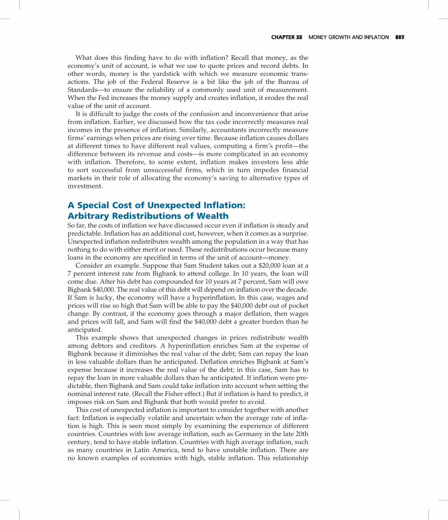
It is difficult to judge the costs of the confusion and inconvenience that arise from inflation. Earlier, we discussed how the tax code incorrectly measures real incomes in the presence of inflation. Similarly, accountants incorrectly measure firms’ earnings when prices are rising over time. Because inflation causes dollars at different times to have different real values, computing a firm’s profit—the difference between its revenue and costs—is more complicated in an economy with inflation. Therefore, to some extent, inflation makes investors less able to sort successful from unsuccessful firms, which in turn impedes financial markets in their role of allocating the economy’s saving to alternative types of investment.

A Special Cost of Unexpected Inflation: Arbitrary Redistributions of WealthSo far, the costs of inflation we have discussed occur even if inflation is steady and predictable. Inflation has an additional cost, however, when it comes as a surprise. Unexpected inflation redistributes wealth among the population in a way that has nothing to do with either merit or need. These redistributions occur because many loans in the economy are specified in terms of the unit of account—money.

Consider an example. Suppose that Sam Student takes out a $20,000 loan at a 7 percent interest rate from Bigbank to attend college. In 10 years, the loan will come due. After his debt has compounded for 10 years at 7 percent, Sam will owe Bigbank $40,000. The real value of this debt will depend on inflation over the decade. If Sam is lucky, the economy will have a hyperinflation. In this case, wages and prices will rise so high that Sam will be able to pay the $40,000 debt out of pocket change. By contrast, if the economy goes through a major deflation, then wages and prices will fall, and Sam will find the $40,000 debt a greater burden than he anticipated.

This example shows that unexpected changes in prices redistribute wealth among debtors and creditors. A hyperinflation enriches Sam at the expense of Bigbank because it diminishes the real value of the debt; Sam can repay the loan in less valuable dollars than he anticipated. Deflation enriches Bigbank at Sam’s expense because it increases the real value of the debt; in this case, Sam has to repay the loan in more valuable dollars than he anticipated. If inflation were pre-dictable, then Bigbank and Sam could take inflation into account when setting the nominal interest rate. (Recall the Fisher effect.) But if inflation is hard to predict, it imposes risk on Sam and Bigbank that both would prefer to avoid.

This cost of unexpected inflation is important to consider together with another fact: Inflation is especially volatile and uncertain when the average rate of infla-tion is high. This is seen most simply by examining the experience of different countries. Countries with low average inflation, such as Germany in the late 20th century, tend to have stable inflation. Countries with high average inflation, such as many countries in Latin America, tend to have unstable inflation. There are no known examples of economies with high, stable inflation. This relationship


between the level and volatility of inflation points to another cost of inflation. If a country pursues a high-inflation monetary policy, it will have to bear not only the costs of high expected inflation but also the arbitrary redistributions of wealth associated with unexpected inflation.

Inflation Is Bad, But Deflation May Be WorseIn recent U.S. history, inflation has been the norm. But the level of prices has fallen at times, such as during the late nineteenth century and early 1930s. Moreover, Japan has experienced declines in its overall price level in recent years. So as we conclude our discussion of the costs of inflation, we should briefly consider the costs of deflation as well.

Some economists have suggested that a small and predictable amount of defla-tion may be desirable. Milton Friedman pointed out that deflation would lower the nominal interest rate (recall the Fisher effect) and that a lower nominal interest rate would reduce the cost of holding money. The shoeleather costs of holding money would, he argued, be minimized by a nominal interest rate close to zero, which in turn would require deflation equal to the real interest rate. This prescrip-tion for moderate deflation is called the Friedman rule.

Yet there are also costs of deflation. Some of these mirror the costs of inflation. For example, just as a rising price level induces menu costs and relative-price variability, so does a falling price level. Moreover, in practice, deflation is rarely as steady and predictable as Friedman recommended. More often, it comes as a surprise, resulting in the redistribution of wealth toward creditors and away from debtors. Because debtors are often poorer, these redistributions in wealth are particularly pernicious.

Perhaps most important, deflation often arises because of broader macro-economic difficulties. As we will see in future chapters, falling prices result when some event, such as a monetary contraction, reduces the overall demand for goods and services in the economy. This fall in aggregate demand can lead to falling incomes and rising unemployment. In other words, deflation is often a symptom of deeper economic problems.

The Wizard of Oz and the Free-Silver Debate

As a child, you probably saw the movie The Wizard of Oz, based on a children’s book written in 1900. The movie and book tell the story of a young girl, Dorothy, who finds herself lost in a strange land far from home. You probably did not know, however, that the story is actually an allegory about U.S. monetary policy in the late 19th century. From 1880 to 1896, the price level in the U.S. economy fell by 23 percent. Because this event was unanticipated, it led to a major redistribution of wealth. Most farmers in the western part of the country were debtors. Their creditors were the bankers in the east. When the price level fell, it caused the real value of these debts to rise, which enriched the banks at the expense of the farmers. According to Populist politicians of the time, the solution to the farmers’ problem was the free coinage of silver. During this period, the United States was operating with a gold standard. The quantity of gold determined the money sup-ply and, thereby, the price level. The free-silver advocates wanted silver, as well


as gold, to be used as money. If adopted, this proposal would have increased the money supply, pushed up the price level, and reduced the real burden of the farmers’ debts. The debate over silver was heated, and it was central to the politics of the 1890s. A common election slogan of the Populists was “We Are Mortgaged. All but Our Votes.” One prominent advocate of free silver was William Jennings Bryan, the Democratic nominee for president in 1896. He is remembered in part for a speech at the Democratic Party’s nominating convention in which he said, “You shall not press down upon the brow of labor this crown of thorns. You shall not crucify mankind upon a cross of gold.” Rarely since then have politicians waxed so poetic about alternative approaches to monetary policy. Nonetheless, Bryan lost the elec-tion to Republican William McKinley, and the United States remained on the gold standard. L. Frank Baum, author of the book The Wonderful Wizard of Oz, was a mid-western journalist. When he sat down to write a story for children, he made the characters represent protagonists in the major political battle of his time. Here is how economic historian Hugh Rockoff, writing in the Journal of Political Economy in 1990, interprets the story:

Dorothy: Traditional American values Toto: Prohibitionist party, also called the Teetotalers Scarecrow: Farmers Tin Woodsman: Industrial workers Cowardly Lion: William Jennings Bryan Munchkins: Citizens of the East Wicked Witch of the East: Grover ClevelandWicked Witch of the West: William McKinley Wizard: Marcus Alonzo Hanna, chairman of the

Republican Party Oz: Abbreviation for ounce of gold Yellow Brick Road: Gold standard

In the end of Baum’s story, Dorothy does find her way home, but it is not by just following the yellow brick road. After a long and perilous journey, she learns that the wizard is incapable of helping her or her friends. Instead, Dorothy finally discovers the magical power of her silver slippers. (When the book was made into a movie in 1939, Dorothy’s slippers were changed from silver to ruby. The Hollywood filmmakers were more interested in showing off the new technology of Technicolor than in telling a story about 19th-century monetary policy.) The Populists lost the debate over the free coinage of silver, but they eventu-ally got the monetary expansion and inflation that they wanted. In 1898, prospec-tors discovered gold near the Klondike River in the Canadian Yukon. Increased supplies of gold also arrived from the mines of South Africa. As a result, the money supply and the price level started to rise in the United States and in other countries operating on the gold standard. Within fifteen years, prices in the United States were back to the levels that had prevailed in the 1880s, and farmers were better able to handle their debts. ■

Quick Quiz List and describe six costs of inflation.

An early debate over monetary policy

© M

gM

/ t

he

ko

baL

co

LLec

tio

n/P

ictu

re d

esk


ConclusionThis chapter discussed the causes and costs of inflation. The primary cause of inflation is simply growth in the quantity of money. When the central bank creates money in large quantities, the value of money falls quickly. To maintain stable prices, the central bank must maintain strict control over the money supply.

The costs of inflation are subtler. They include shoeleather costs, menu costs, increased variability of relative prices, unintended changes in tax liabilities, confusion and inconvenience, and arbitrary redistributions of wealth. Are these costs, in total, large or small? All economists agree that they become huge during hyperinflation. But their size for moderate inflation—when prices rise by less than 10 percent per year—is more open to debate.

Although this chapter presented many of the most important lessons about infla-tion, the discussion is incomplete. When the central bank reduces the rate of money growth, prices rise less rapidly, as the quantity theory suggests. Yet as the economy makes the transition to this lower inflation rate, the change in monetary policy will

Bernanke and the Beast By N. GreGory MaNkiw

Is galloping inflation around the corner? Without doubt, the United States is exhib-

iting some of the classic precursors to out-of-control inflation. But a deeper look suggests that the story is not so simple. Let’s start with first principles. One basic lesson of economics is that prices rise when the government creates an excessive amount of money. In other words, inflation occurs when too much money is chasing too few goods. A second lesson is that governments resort to rapid monetary growth because they face fiscal problems. When government

spending exceeds tax collection, policy mak-ers sometimes turn to their central banks, which essentially print money to cover the budget shortfall. Those two lessons go a long way toward explaining history’s hyperinflations, like those experienced by Germany in the 1920s or by Zimbabwe recently. Is the United States about to go down this route? To be sure, we have large budget deficits and ample money growth. The federal gov-ernment’s budget deficit was $390 billion in the first quarter of fiscal 2010, or about 11 percent of gross domestic product. Such a large deficit was unimaginable just a few years ago. The Federal Reserve has also been rap-idly creating money. The monetary base—meaning currency plus bank reserves—is the money-supply measure that the Fed

controls most directly. That figure has more than doubled over the last two years. Yet, despite having the two classic ingre-dients for high inflation, the United States has experienced only benign price increases. Over the last year, the core Consumer Price Index, excluding food and energy, has risen by less than 2 percent. And long-term inter-est rates remain relatively low, suggesting that the bond market isn’t terribly worried about inflation. What gives? Part of the answer is that while we have large budget deficits and rapid money growth, one isn’t causing the other. Ben S. Bernanke, the Fed chairman, has been printing money not to finance President Obama’s spending but to rescue the finan-cial system and prop up a weak economy. Moreover, banks have been happy to hold much of that new money as excess

Inflationary ThreatsIn the aftermath of the financial crisis and economic downturn of 2008 and 2009, some observers of the U.S. economy started worrying about inflation.

in the news


SuMMARy

reserves. In normal times when the Fed expands the monetary base, banks lend that money, and other money-supply measures grow in parallel. But these are not normal times. With banks content holding idle cash, the broad measure called M2 (including cur-rency and deposits in checking and savings accounts) has grown in the last two years at an annual rate of only 6 percent. As the economy recovers, banks may start lending out some of their hoards of reserves. That could lead to faster growth in broader money-supply measures and, eventually, to substantial inflation. But the Fed has the tools it needs to prevent that outcome. For one, it can sell the large portfolio of mortgage-backed securities and other assets it has accumulated over the last cou-ple of years. When the private purchasers of those assets paid up, they would drain reserves from the banking system. And as a result of legislative changes in October 2008, the Fed has a new tool: it can pay interest on reserves. With short-term interest rates currently near zero, this tool has been largely irrelevant. But as the economy recovers and interest rates rise, the Fed can increase the interest rate it pays banks to

hold reserves as well. Higher interest on reserves would discourage bank lending and prevent the huge expansion in the monetary base from becoming inflationary. But will Mr. Bernanke and his colleagues make enough use of these instruments when needed? Most likely they will, but there are still several reasons for doubt. First, a little bit of inflation might not be so bad. Mr. Bernanke and company could decide that letting prices rise and thereby reducing the real cost of borrowing might help stimulate a moribund economy. The trick is getting enough inflation to help the economy recover without losing control of the process. Fine-tuning is hard to do. Second, the Fed could easily over-estimate the economy’s potential growth. In light of the large fiscal imbalance over

which Mr. Obama is presiding, it’s a good bet he will end up raising taxes for most Americans in coming years. Higher tax rates mean reduced work incentives and lower potential output. If the Fed fails to account for this change, it could try to promote more growth than the economy can sustain, caus-ing inflation to rise. Finally, even if the Fed is committed to low inflation and recognizes the challenges ahead, politics could constrain its policy choices. Raising interest rates to deal with impending inflationary pressures is never popular, and after the recent financial crisis, Mr. Bernanke cannot draw on a boundless reservoir of good will. As the economy recovers, responding quickly and fully to inflation threats may prove hard in the face of public opposition. Investors snapping up 30-year Treasury bonds paying less than 5 percent are bet-ting that the Fed will keep these inflation risks in check. They are probably right. But because current monetary and fiscal policy is so far outside the bounds of historical norms, it’s hard for anyone to be sure. A decade from now, we may look back at today’s bond market as the irrational exu-berance of this era.

Source: New York Times, January 17, 2010.

• The overall level of prices in an economy adjusts to bring money supply and money demand into balance. When the central bank increases the supply of money, it causes the price level to rise. Persistent growth in the quantity of money supplied leads to continuing inflation.

• The principle of monetary neutrality asserts that changes in the quantity of money influence nominal variables but not real variables. Most economists believe that monetary neutrality approximately describes the behavior of the economy in the long run.

have disruptive effects on production and employment. That is, even though mone-tary policy is neutral in the long run, it has profound effects on real variables in the short run. Later in this book we will examine the reasons for short-run monetary nonneutrality to enhance our understanding of the causes and costs of inflation.

© d

av

id g

. k

Lein


• A government can pay for some of its spending simply by printing money. When countries rely heavily on this “inflation tax,” the result is hyperinflation.

• One application of the principle of monetary neutrality is the Fisher effect. According to the Fisher effect, when the inflation rate rises, the nominal interest rate rises by the same amount so that the real interest rate remains the same.

• Many people think that inflation makes them poorer because it raises the cost of what they buy. This view is a fallacy, however, because inflation also raises nominal incomes.

• Economists have identified six costs of inflation: shoeleather costs associated with reduced money holdings, menu costs associated with more frequent adjustment of prices, increased variability of relative prices, unintended changes in tax liabilities due to nonindexation of the tax code, confusion and inconvenience resulting from a changing unit of account, and arbitrary redistributions of wealth between debtors and creditors. Many of these costs are large during hyperinflation, but the size of these costs for moderate inflation is less clear.

KEy CoNCEPTS

QuESTIoNS FoR REVIEw

1. Explain how an increase in the price level affects the real value of money.

2. According to the quantity theory of money, what is the effect of an increase in the quantity of money?

3. Explain the difference between nominal and real variables and give two examples of each. According to the principle of monetary neutrality, which variables are affected by changes in the quantity of money?

4. In what sense is inflation like a tax? How does thinking about inflation as a tax help explain hyperinflation?

5. According to the Fisher effect, how does an increase in the inflation rate affect the real interest rate and the nominal interest rate?

6. What are the costs of inflation? Which of these costs do you think are most important for the U.S. economy?

7. If inflation is less than expected, who benefits—debtors or creditors? Explain.

PRoBLEMS AND APPLICATIoNS

1. Suppose that this year’s money supply is $500 billion, nominal GDP is $10 trillion, and real GDP is $5 trillion.a. What is the price level? What is the velocity

of money?b. Suppose that velocity is constant and the

economy’s output of goods and services rises by 5 percent each year. What will

happen to nominal GDP and the price level next year if the Fed keeps the money supply constant?

c. What money supply should the Fed set next year if it wants to keep the price level stable?

d. What money supply should the Fed set next year if it wants inflation of 10 percent?

266 PART V Money and Prices in the Long run

quantity theory of money, p. 247nominal variables, p. 249real variables, p. 249classical dichotomy, p. 249

monetary neutrality, p. 250velocity of money, p. 250quantity equation, p. 251inflation tax, p. 253

Fisher effect, p. 255shoeleather costs, p. 257menu costs, p. 258

370 PART VI Money and Prices in the Long run




482 PART VIII Money and Prices in the Long run




PART X Money and Prices in the Long run666




2. Suppose that changes in bank regulations expand the availability of credit cards so that people need to hold less cash. a. How does this event affect the demand for

money?b. If the Fed does not respond to this event,

what will happen to the price level?c. If the Fed wants to keep the price level stable,

what should it do? 3. It is sometimes suggested that the Federal

Reserve should try to achieve zero inflation. If we assume that velocity is constant, does this zero-inflation goal require that the rate of money growth equal zero? If yes, explain why. If no, explain what the rate of money growth should equal.

4. Suppose that a country’s inflation rate increases sharply. What happens to the inflation tax on the holders of money? Why is wealth that is held in savings accounts not subject to a change in the inflation tax? Can you think of any way holders of savings accounts are hurt by the increase in the inflation rate?

5. Hyperinflations are extremely rare in countries whose central banks are independent of the rest of the government. Why might this be so?

6. Let’s consider the effects of inflation in an economy composed of only two people: Bob, a bean farmer, and Rita, a rice farmer. Bob and Rita both always consume equal amounts of rice and beans. In 2010, the price of beans was $1, and the price of rice was $3.a. Suppose that in 2011 the price of beans was

$2 and the price of rice was $6. What was inflation? Was Bob better off, worse off, or unaffected by the changes in prices? What about Rita?

b. Now suppose that in 2011 the price of beans was $2 and the price of rice was $4. What was inflation? Was Bob better off, worse off, or unaffected by the changes in prices? What about Rita?

c. Finally, suppose that in 2011 the price of beans was $2 and the price of rice was $1.50. What was inflation? Was Bob better off, worse off, or unaffected by the changes in prices? What about Rita?

d. What matters more to Bob and Rita—the overall inflation rate or the relative price of rice and beans?

7. If the tax rate is 40 percent, compute the before-tax real interest rate and the after-tax real interest rate in each of the following cases.a. The nominal interest rate is 10 percent, and

the inflation rate is 5 percent.b. The nominal interest rate is 6 percent, and the

inflation rate is 2 percent.c. The nominal interest rate is 4 percent, and the

inflation rate is 1 percent. 8. What are your shoeleather costs of going to

the bank? How might you measure these costs in dollars? How do you think the shoeleather costs of your college president differ from your own?

9. Recall that money serves three functions in the economy. What are those functions? How does inflation affect the ability of money to serve each of these functions?

10. Suppose that people expect inflation to equal 3 percent, but in fact, prices rise by 5 percent. Describe how this unexpectedly high inflation rate would help or hurt the following:a. the governmentb. a homeowner with a fixed-rate mortgagec. a union worker in the second year of a labor

contractd. a college that has invested some of its

endowment in government bonds 11. Explain one harm associated with

unexpected inflation that is not associated with expected inflation. Then explain one harm associated with both expected and unexpected inflation.

12. Explain whether the following statements are true, false, or uncertain.a. “Inflation hurts borrowers and helps lenders,

because borrowers must pay a higher rate of interest.”

b. “If prices change in a way that leaves the overall price level unchanged, then no one is made better or worse off.”

c. “Inflation does not reduce the purchasing power of most workers.”

For further information on topics in this chapter, additional problems, applications, examples, online quizzes, and more, please visit our website at www.cengage.com/economics/mankiw.

267CHAPTER 12 Money growth and inFLation 371CHAPTER 17 Money growth and inFLation 483CHAPTER 22 Money growth and inFLationCHAPTER 30 Money growth and inFLation 667

The Classical Theory of Inflation -...

Documents

Transcript of The Classical Theory of Inflation -...