The Chaffey Dam Story

Final report for CRCFE projects B.202 and B.203

Edited by Bradford Sherman, CSIRO Land & Water

Contributing authors:

Bradford Sherman CSIRO Land and WaterPhillip Ford CSIRO Land and WaterPat Hatton CSIRO Land and WaterJohnWhittington CRCFEDamian Green CRCFEDarren Baldwin MDFRCRod Oliver MDFRCRuss Shiel MDFRCJason van Berkel Water Studies Centre, Monash UniversityRon Beckett Water Studies Centre, Monash UniversityLeigh Grey University of CanberraBill Maher University of Canberra

- i -

1 EXECUTIVE SUMMARY. . . . . . . . . . . . . . . . . . . . . . . . . . . . . . . . . . . . . . . . . . . . . . . . . . . . . . . . . . . . . . . . . . . . . . . . . . 1

2 GLOSSARY OF TERMS. . . . . . . . . . . . . . . . . . . . . . . . . . . . . . . . . . . . . . . . . . . . . . . . . . . . . . . . . . . . . . . . . . . . . . . . . . . 5

3 INTRODUCTION. . . . . . . . . . . . . . . . . . . . . . . . . . . . . . . . . . . . . . . . . . . . . . . . . . . . . . . . . . . . . . . . . . . . . . . . . . . . . . . . . . 1 1

3.1 WHY CHAFFEY RESERVOIR?............................................................................................. 12

4 SITE DESCRIPTION . . . . . . . . . . . . . . . . . . . . . . . . . . . . . . . . . . . . . . . . . . . . . . . . . . . . . . . . . . . . . . . . . . . . . . . . . . . . . 1 5

4.1 LOCATION .................................................................................................................... 154.2 FACILITIES.................................................................................................................... 16

4.2.1 Historical data archive ............................................................................................. 164.2.2 Destratification system............................................................................................ 161.1.3 Multilevel outlet structure........................................................................................ 19

5 METHODS. . . . . . . . . . . . . . . . . . . . . . . . . . . . . . . . . . . . . . . . . . . . . . . . . . . . . . . . . . . . . . . . . . . . . . . . . . . . . . . . . . . . . . . . . . 2 1

5.1 ROUTINE MONITORING PROGRAM...................................................................................... 215.2 INTENSIVE SAMPLING PROGRAM ........................................................................................ 21

6 CLIMATE. . . . . . . . . . . . . . . . . . . . . . . . . . . . . . . . . . . . . . . . . . . . . . . . . . . . . . . . . . . . . . . . . . . . . . . . . . . . . . . . . . . . . . . . . . . 2 4

6.1 METEOROLOGY ............................................................................................................. 246.2 INFLOWS AND OUTFLOWS................................................................................................. 276.3 RESERVOIR HEAT AND WATER BUDGETS ............................................................................. 28

6.3.1 Water budget ......................................................................................................... 281.1.2 Heat budget ........................................................................................................... 301.1.3 Conclusion ........................................................................................................... 31

7 TRANSPORT PROCESSES. . . . . . . . . . . . . . . . . . . . . . . . . . . . . . . . . . . . . . . . . . . . . . . . . . . . . . . . . . . . . . . . . . . . . 3 3

7.1 INFLOW EVENTS............................................................................................................. 337.2 SURFACE LAYER DYNAMICS.............................................................................................. 351.3 IMPACT OF DESTRATIFICATION .......................................................................................... 411.4 TURBULENT DIFFUSION (HYPOLIMNION TO EPILIMNION)......................................................... 431.5 DIFFERENTIAL COOLING .................................................................................................. 441.6 SUMMARY .................................................................................................................... 47

8 THE NUTRIENT STORY . . . . . . . . . . . . . . . . . . . . . . . . . . . . . . . . . . . . . . . . . . . . . . . . . . . . . . . . . . . . . . . . . . . . . . . . 4 9

8.1 INTRODUCTION.............................................................................................................. 498.2 SEDIMENT CHEMISTRY .................................................................................................... 50

8.2.1 Methods ............................................................................................................... 508.2.2 Reservoir siltation.................................................................................................. 528.2.3 Elemental and mineralogical composition of the sediments............................................. 528.2.4 Organic carbon in the sediments ................................................................................ 538.2.5 Sediment traps and the downward flux of organic carbon ................................................ 558.2.6 Sediment phosphorus speciation................................................................................ 55

8.2.6.1 Speciation by selective extraction .. . . . . . . . . . . . . . . . . . . . . . . . . . . . . . . . . . . . . . . . . . . . . . . . . . . . . . . . . . . . . . . . . . . . . . 558.2.6.2 Sediment P speciation by 31P nmr (nuclear magnetic resonance).. . . . . . . . . . . . . . . . . . . . . . . . . . . . . . . . . . . 56

8.2.7 Desiccation and sediment phosphorus cycling .............................................................. 568.2.7.1 The effects of desiccation/oxidation on the sediment’s capacity to adsorb P under oxicconditions 578.2.7.2 The effects of desiccation/oxidation on the potential for bacterially mediated P release fromsediments. 58

8.3 WATER COLUMN CHEMISTRY ............................................................................................ 598.3.1 Methods ............................................................................................................... 591.1.2 Historical trends in water chemistry ........................................................................... 611.1.3 Major ion chemistry ............................................................................................... 651.1.4 Water column P speciation....................................................................................... 66

1.1.4.1 Speciation by weak anion exchange chromatography... . . . . . . . . . . . . . . . . . . . . . . . . . . . . . . . . . . . . . . . . . . . . . 661.1.4.2 Speciation of particle-bound P in water column... . . . . . . . . . . . . . . . . . . . . . . . . . . . . . . . . . . . . . . . . . . . . . . . . . . . . . 68

1.1.5 Iron and manganese................................................................................................. 691.1.5.1 Fe2+ size speciation. . . . . . . . . . . . . . . . . . . . . . . . . . . . . . . . . . . . . . . . . . . . . . . . . . . . . . . . . . . . . . . . . . . . . . . . . . . . . . . . . . . . . . . . . . 70

- ii -

1.1.5.2 Mn2+ size speciation.. . . . . . . . . . . . . . . . . . . . . . . . . . . . . . . . . . . . . . . . . . . . . . . . . . . . . . . . . . . . . . . . . . . . . . . . . . . . . . . . . . . . . . . . 701.1.5.3 Kinetics of the reductive dissolution and oxidation of iron and manganese. . . . . . . . . . . . . . . . . . . . . . 711.1.5.4 Crystalline structure of colloids.. . . . . . . . . . . . . . . . . . . . . . . . . . . . . . . . . . . . . . . . . . . . . . . . . . . . . . . . . . . . . . . . . . . . . . . . . . 72

1.1.6 Examination of dissolved organic matter by weak-anion exchange chromatography. ............ 731.1.7 Oxygen dynamics................................................................................................... 74

1.4 INFLOW (PEEL R.) CHEMISTRY.......................................................................................... 761.4.1 Methods ............................................................................................................... 761.4.2 Relationships between nutrient inputs and suspended sediments in the Peel River inflows.... 77

1.5 NUTRIENT BUDGET......................................................................................................... 791.1.1 Peel River event flow nutrient loads........................................................................... 811.1.2 Peel River base flow nutrient loads............................................................................ 821.1.3 Mass balance results ............................................................................................... 82

1.1.1.1 Internal nutrient loads.. . . . . . . . . . . . . . . . . . . . . . . . . . . . . . . . . . . . . . . . . . . . . . . . . . . . . . . . . . . . . . . . . . . . . . . . . . . . . . . . . . . . . . 841.1.4 Benthic chamber measurements of internal nutrient loads from sediments.......................... 84

1.6 CONCLUSIONS ............................................................................................................... 85

9 TROPHIC DYNAMICS - ALGAL SPECIES SUCCESSION . . . . . . . . . . . . . . . . . . . . . . . . . . . . . . 8 7

9.1 METHODOLOGY............................................................................................................. 879.1.1 Elbow grabs vs 5 m-integrated sampling..................................................................... 889.1.2 Biovolume vs chlorophyll-a ..................................................................................... 88

1.2 TRENDS IN ALGAL ABUNDANCE......................................................................................... 891.2.1 Species composition............................................................................................... 891.2.2 Interannual biovolume variability .............................................................................. 921.2.3 Seasonal biovolume trends....................................................................................... 92

1.2.3.1 Blue-green algae.. . . . . . . . . . . . . . . . . . . . . . . . . . . . . . . . . . . . . . . . . . . . . . . . . . . . . . . . . . . . . . . . . . . . . . . . . . . . . . . . . . . . . . . . . . . . . 931.2.3.2 Green algae .. . . . . . . . . . . . . . . . . . . . . . . . . . . . . . . . . . . . . . . . . . . . . . . . . . . . . . . . . . . . . . . . . . . . . . . . . . . . . . . . . . . . . . . . . . . . . . . . . . . 931.2.3.3 Dinoflagellates .. . . . . . . . . . . . . . . . . . . . . . . . . . . . . . . . . . . . . . . . . . . . . . . . . . . . . . . . . . . . . . . . . . . . . . . . . . . . . . . . . . . . . . . . . . . . . . 931.2.3.4 Cryptomonads .. . . . . . . . . . . . . . . . . . . . . . . . . . . . . . . . . . . . . . . . . . . . . . . . . . . . . . . . . . . . . . . . . . . . . . . . . . . . . . . . . . . . . . . . . . . . . . . 941.2.3.5 Diatoms... . . . . . . . . . . . . . . . . . . . . . . . . . . . . . . . . . . . . . . . . . . . . . . . . . . . . . . . . . . . . . . . . . . . . . . . . . . . . . . . . . . . . . . . . . . . . . . . . . . . . . 941.2.3.6 Is there a generalised annual successional sequence at Chaffey Dam?... . . . . . . . . . . . . . . . . . . . . . . . . . . . 94

1.2.4 Nutrients and algal growth ....................................................................................... 951.2.4.1 Algal growth ‘events’ . . . . . . . . . . . . . . . . . . . . . . . . . . . . . . . . . . . . . . . . . . . . . . . . . . . . . . . . . . . . . . . . . . . . . . . . . . . . . . . . . . . . . . . 961.1.1.2 Hypolimnetic P and algal biomass .. . . . . . . . . . . . . . . . . . . . . . . . . . . . . . . . . . . . . . . . . . . . . . . . . . . . . . . . . . . . . . . . . . . . . . 991.1.1.3 Algal physiology and bioassays.. . . . . . . . . . . . . . . . . . . . . . . . . . . . . . . . . . . . . . . . . . . . . . . . . . . . . . . . . . . . . . . . . . . . . . . .1001.1.1.4 Summary ... . . . . . . . . . . . . . . . . . . . . . . . . . . . . . . . . . . . . . . . . . . . . . . . . . . . . . . . . . . . . . . . . . . . . . . . . . . . . . . . . . . . . . . . . . . . . . . . . . . .101

1.3 LIGHT LIMITATION........................................................................................................1021.3.1 The underwater light environment.............................................................................1021.3.2 Light dose in the surface mixed layer.........................................................................1021.1.3 Light intensity vs net phytoplankton growth rate ........................................................104

1.1.3.1 Methods.. . . . . . . . . . . . . . . . . . . . . . . . . . . . . . . . . . . . . . . . . . . . . . . . . . . . . . . . . . . . . . . . . . . . . . . . . . . . . . . . . . . . . . . . . . . . . . . . . . . . . .1041.1.3.2 Results . . . . . . . . . . . . . . . . . . . . . . . . . . . . . . . . . . . . . . . . . . . . . . . . . . . . . . . . . . . . . . . . . . . . . . . . . . . . . . . . . . . . . . . . . . . . . . . . . . . . . . . .104

1.1.4 Phytoplankton photophysiology ..............................................................................1051.1.4.1 Methods.. . . . . . . . . . . . . . . . . . . . . . . . . . . . . . . . . . . . . . . . . . . . . . . . . . . . . . . . . . . . . . . . . . . . . . . . . . . . . . . . . . . . . . . . . . . . . . . . . . . . . .1061.1.1.2 Species-specific photosynthetic parameters .. . . . . . . . . . . . . . . . . . . . . . . . . . . . . . . . . . . . . . . . . . . . . . . . . . . . . . . . .1061.1.1.3 Coupling between photosynthesis and surface layer dynamics .. . . . . . . . . . . . . . . . . . . . . . . . . . . . . . . . . . .107

1.1.5 Buoyancy and motility mechanisms to avoid sedimentation and optimise light capture .......1081.1.1.1 Relationship between light, nutrients and buoyancy ... . . . . . . . . . . . . . . . . . . . . . . . . . . . . . . . . . . . . . . . . . . . .1091.1.1.2 Algal migration by swimming ... . . . . . . . . . . . . . . . . . . . . . . . . . . . . . . . . . . . . . . . . . . . . . . . . . . . . . . . . . . . . . . . . . . . . . . . .1101.1.1.3 Algal migration in a turbulent environment .. . . . . . . . . . . . . . . . . . . . . . . . . . . . . . . . . . . . . . . . . . . . . . . . . . . . . . . . . .111

1.1.6 Sedimentation.......................................................................................................1141.1.7 Can artificial destratification light limit algal growth?..................................................114

1.4 ZOOPLANKTON.............................................................................................................1151.4.1 Summary & overview............................................................................................116

1.5 SUMMARY ...................................................................................................................118

1 0 MANAGEMENT IMPLICATIONS. . . . . . . . . . . . . . . . . . . . . . . . . . . . . . . . . . . . . . . . . . . . . . . . . . . . . . . . . . 1 2 1

10.1 OPERATIONAL CONSIDERATIONS FOR ARTIFICIAL DESTRATIFICATION.......................................12110.1.1 Effects of the destratification system on water column chemistry....................................12110.1.2 Thermal effects of destratification .............................................................................122

10.2 IN-RESERVOIR PHOSPHORUS REDUCTION STRATEGIES ............................................................12210.2.1 Selective withdrawal from the hypolimnion................................................................12210.2.2 Destratification .....................................................................................................122

- iii -

10.2.3 Hypolimnetic oxygenation......................................................................................1231.1.4 Sediment remediation.............................................................................................1241.1.5 Fe3+ dosing ..........................................................................................................1241.1.6 Sediment dessication and oxidation as control strategies for P release...............................125

10.3 CATCHMENT MANAGEMENT............................................................................................12510.3.1 Control of sulphate entry into the Dam. ....................................................................125

10.4 LIGHT LIMITATION STRATEGIES .......................................................................................12610.4.1 Surface impellers to light-limit algal growth ..............................................................126

1 1 APPENDIX A – DESTRATIFICATION EXPERIMENTS . . . . . . . . . . . . . . . . . . . . . . . . . . . . . . 1 2 7

11.1 THE EFFECT OF ARTIFICIAL MIXING ON PHYTOPLANKTON ABUNDANCE AND COMMUNITY

COMPOSITION. ..........................................................................................................................12711.2 TRIAL 1. 22 FEB 95 TO 29 MAR 95..................................................................................12711.3 TRIAL 2 4 OCT 95 TO 28 OCT 95 .....................................................................................12711.4 TRIAL 3 11-1-96 TO 13 FEB 96........................................................................................12711.5 TRIAL 4 24 NOV 96 TO 24 DEC 96...................................................................................12811.6 TRIAL 5 13 APR 97 TO 23 APR 97 ....................................................................................12811.7 CONCLUSIONS OF SHORT TERM MIXING..............................................................................128

1 2 APPENDIX B - ZOOPLANKTON OBSERVATIONS BY YEAR . . . . . . . . . . . . . . . . . . . . . . 1 2 9

12.1 12 SEP 95 – 26 DEC 95 (N=17 DATES X 3 SITES) ..................................................................12912.2 02 JAN 96 – 30 DEC 96 (N=52 DATES X 3 SITES)..................................................................12912.3 JAN 97 – 09 DEC 97 (N=49 DATES X 3 SITES) ......................................................................130

1 3 REFERENCES. . . . . . . . . . . . . . . . . . . . . . . . . . . . . . . . . . . . . . . . . . . . . . . . . . . . . . . . . . . . . . . . . . . . . . . . . . . . . . . . . 1 3 3

Figure 4.1 Map of New South Wales showing approximate location of Chaffey reservoir. ____ 15

Figure 4.2 Temperature profile at Chaffey Reservoir on 2 Feb 1993. _____________________ 17

Figure 4.3 DYRESM simulated temperature profiles for compressor airflow rates of 300, 900 and1350 L s-1. Date format is yyddd. Compressor operation commences 88001 (1 Jan 1988)._ 19

Figure 4.4 Location of top and bottom of outlet for water released from Chaffey Dam.________ 20

Figure 5.1 Location of algal sampling sites (A1-A5), meterological station (Met), thermistorchains (TC1, TC2), CTDO casts (Stn 1 – Stn3, 11-13) and sediment samples for speciationand oxidation experiments. The 518 m contour is the water level when the reservoir isnearly full (95% of capacity). The 506 m contour was the minimum water level duringthe project. See Table 5.1 for details. ____________________________________ 22

Figure 6.1 Minimum (hatched), maximum (gray), and mean (black) values of air temperature,shortwave radiation, downwelling longwave radiation, relative humidity, and windspeed at Chaffey Reservoir. __________________________________________ 25

Figure 6.2 Daily values during the study period of net heat flux (a), shortwave radiation (b), netlongwave radiation (c), and sensible and latent heat flux (d).__________________ 26

Figure 6.3 Monthly Peel River flows into Chaffey Reservoir.__________________________ 27

Figure 6.4 a) Reservoir level (solid line), daily releases from Chaffey Reservoir (grey shadedregion), and mean monthly Peel River inflow (black bars) during the project. b)Historical reservoir level 1985 - 1998. ___________________________________ 28

Figure 6.5 a) Components of the water budget at Chaffey Reservoir. Observed change in reservoirvolume, dV, net inflow, dQ, and net rainfall + evaporation. b) Monthly (∆V error) andcumulative (∑ ∆V error) errors in the water budget. _________________________ 29

Figure 6.6 a) Predicted and observed daily reservoir heat contents. b) Monthly observed change inheat content (∆HCobs), predicted change due to inflow (Hin), outflow (Hout), and surfaceheat trnasfers + rainfall (Hsurf + Hrain) c) Difference between observed and predictedheat content change (∆HCerror); heat content associated with the water balance error(∆HQerror); and residual error (∆HCresidual) after correction for the water balance error. d)Residual error as a proportion of the reservoir heat content. ___________________ 32

- iv -

Figure 7.1 Conductivity (top) and FRP and TP (bottom) profiles measured at Chaffey Reservoirbefore and after the Feb 97 inflow. Conductivity profiles are offset by 0.002 S m-1; grayvertical lines are located at 0.031 S m-1 for each profile. The trajectory of the maximumsurface layer depth between profile is shown by the heavy line in the upper figure. _ 35

Figure 7.2 TDFO profile taken 27 Mar 96. 90% of chl-a was located above the 0.04 °C temperaturechange at 4.5 m (dashed line). The dissolved oxygen profile shows that the homogenousregion is between the surface and 3.5 m, the depth at the bottom of the unstabletemperature distribution and corresponding to the top of the chl-a gradient. Figure fromSherman et al. (1999). _______________________________________________ 37

Figure 7.3 Average (shaded area) and maximum (solid line) daily surface layer depth, h,computed from thermistor chain data during summer and winter periods from 1995 to1997. Gaps indicate periods of missing record. Solid black bars denote operation of thedestratifier. ______________________________________________________ 39

Figure 7.4 Average and maximum surface mixed layer depth, h, (top) and average u*, w*, q*(bottom). Data shown are for a composite day averaged from 644 days of 10-minutedata. ___________________________________________________________ 40

Figure 7.5 Schematic diagram of the circulation patterns established by artificialdestratification at Chaffey Reservoir. Also shown is the velocity profile measured _ 41

Figure 7.6 Temperature profiles at Chaffey Dam during the operation of the destratifier from 4 -28 Oct 1995 and 11 Jan - 13 Feb 1996. A 3 - 4 m deep surface layer persisted during theOctober 1995 operation and in January 1996 the layer ________________________ 42

Figure 7.7 Schematic diagram of circulation induced by differential cooling. Reproduced fromWells and Sherman (submitted). _______________________________________ 45

Figure 7.8 CTDO temperature profiles during the winters of 1995 and 1996 reveal a persistent coldintrusion along the bottommost 4.5-5 m of the reservoir. ______________________ 46

Figure 7.9 TDFO and quantum yield profiles in Chaffey Reservoir on 16 Feb 96. The bold line inthe fluorescence plot is a moving average of the raw fluorescence data (gray line). __ 47

Figure 8.1 Locations of sediment samples collected from Chaffey Reservoir. Some sites not shown.51

Figure 8.2 Profiles of δ13C, δ 18O, and δ15N (top) and % C, %N, and %N x10 (bottom) in a sedimentcore taken from the centre of the south basin of Chaffey Reservoir on 5 March 1997.__ 54

Figure 8.3 P-speciation of Chaffey Reservoir sediments using modified selective extraction. FromBaldwin (1996b).___________________________________________________ 56

Figure 8.4 The ‘Ferrous’ Wheel ________________________________________________ 58

Figure 8.5 Annual number of visits to Station 1 to collect samples for chemical analysis. ______ 60

Figure 8.6 Seasonal changes in nutrient concentrations in the surface layer (0 – 5 m, solid line) andhypolimnion (> 12 m depth, shaded region) of Chaffey Reservoir from winter 1985 towinter 1997. From top to bottom, nitrate + nitrite ___________________________ 62

Figure 8.7 Hypolimnetic (> 12 m depth, shaded region) and surface layer (0 – 5 m, solid line)nutrient and dissolved oxygen concentrations during this project ________________ 64

Figure 8.8 Major cations (top) and anions (bottom) in the water column at Chaffey reservoir.___ 66

Figure 8.9 Total (gray) and reactive (white) phosphorus speciation in water column samples asdetermined by weak anion exchange chromatography._______________________ 67

Figure 8.10 Filterable Fe2+ and Mn2+ Profile when stratified during April 1997 at Station 1. ____ 71

Figure 8.11 Figure 3 X-ray diffraction of Chaffey Reservoir anoxic particles. _______________ 72

Figure 8.12 X-ray diffraction of Chaffey Reservoir oxidized particles. ___________________ 72

Figure 8.13 Chromatograms of dissolved organic matter (DOM) speciation in Chaffey Reservoir. 74

Figure 8.14 Top) Hypolimnetic oxygen demand following the onset of persistent stratification.Dates on top of bars indicate the period used for the calculation. Bottom) Mean surface

- v -

(0 - 5 m, solid line) and hypolimnetic (> 12 m, shaded region) dissolved oxygenconcentrations from the weekly CTDO casts. ______________________________ 75

Figure 8.15 Correlation between suspended sediment and turbidity in samples collected from thePeel River at Taroona. 3 outliers have been eliminated from the correlation. ______ 77

Figure 8.16 Correlations between turbidity and NOx, NH4, TKN, TN, FRP, and TP for all datawhere the turbidity was within detection limits (< 1000 NTU). ________________ 78

Figure 8.17 Correlations between total suspended sediment and NOx, NH4, TKN, TN, FRP, and TPfor the Peel River at Taroona. _________________________________________ 79

Figure 8.18 External loads of TP and FRP from the Peel River and the observed change in the totalmass of TP (∆TP) and FRP (∆FRP) in the water column of _____________________ 83

Figure 9.1 Weekly total algal biovolume as reported by DLWC and CRCFE and chlorophyll-aconcentration during the project. DLWC data are from single samples collected from 0.25m depth at Stn 1. CRCFE and chlorophyll data are averages of 5-m integrated samplescollected at 5 sites around the reservoir.__________________________________ 89

Figure 9.2 Algal cell volume (mm3 L-1), averaged monthly, for the major species of algae atChaffey Dam. a) Cyanobacteria, b) Dinoflagellates, c) Chlorophycaea, d)Cryptomonads. These 8 species comprise 88% of the total phytoplankton population.Numbers indicate maximum biomass for peaks that extend beyond the limits of the y-axis. Data collected by DLWC. ________________________________________ 91

Figure 9.3 Algal biovolume and surface layer (0 – 5 m) FRP, NH4, and NOx concentrations during1995-1997. Light shaded vertical bars denote operation of the destratifier. Algal datacollected by CRCFE. ________________________________________________ 95

Figure 9.4 Response of Anabaena and Microcystis populations to changes in surface layerconcentrations of FRP, NOx and NH4 during January – June 1996. ________________ 97

Figure 9.5 Response of Anabaena and Microcystis populations to changes in surface layerconcentrations of FRP, NOx and NH4 during January – June 1997. ________________ 98

Figure 9.6 Mean annual algal biovolume vs hypolimnetic TP just prior to turnover at the start ofthe algal growing year. Open circles denote years that the destratifier was operated.

100

Figure 9.7 Top) Algal biovolume and Peel River discharge during the project. Numbers indicatedaily mean discharge when data extend beyond the limit of the y-axis. Bottom)Average daily irradiance experienced by algae in the surface layer using the 10-minutesurface layer depth data from the thermistor chains (grey shaded region) and themaximum diurnal SML depth (solid line). _______________________________ 103

Figure 9.8 Conceptual diagram of the parameters measured in the light-growth experiments._ 104

Figure 9.9 Top) PAR (grey shaded area) and wind speed (line) during 26-27 Nov 1996. Bottom)Surface mixed layer (SML) depth (grey shaded area) and ∆Φ at 5 depths for the sameperiod. Measurements were made when the algal community was dominated by thegreen alga Oocystis sp.. _____________________________________________ 108

Figure 9.10 Averaged fluorescence profiles collected from Chaffey Reservoir. 11:34-13:04 9 Jan 1996(solid line, mean q* = 0.002 m s-1 during profiling), 17:52-19:00 11 Jan 1996 (long dashedline, mean q* = 0.007 m s-1 during profiling) and 13:32-15:02 14 Jan 1996 (short dashedline, mean q* = 0.004 m s-1 during profiling). ______________________________ 111

Figure 9.11 Turbulent velocity scale, q*, and SML depth during April 1997. The horizontal line inthe upper plot is at q* = 8.3 x 10-3 m s-1. __________________________________ 112

Figure 9.12 Meteorological and water column conditions measured at Chaffey Reservoir. 10 minuteaveraged data for a) incident irradiance, PAR, µmol photons m-2 s-1 ; b) wind speed, m s-

1; c) mixed-layer depth, h, m; d) turbulent velocity scale in the mixed-layer, q*, m s-1,for the period 9 Jan 1996 to 15 Jan 1996. __________________________________ 113

Figure 9.13 Population densities of the most numerous zooplankton species found in ChaffeyReservoir relative to the timing of algal growth. Dark shading is the 5 site meanchlorophyll-a in the top 5 m and the light shading is the corresponding biovolume. a)

- vi -

Asplanchna priodonta, Ceriodaphnia cf. dubia and Chydorus sp. b) Daphnia carinataand Daphnia lumholtzi . c) The ciliates Halteria and Strombidiu . ____________ 117

- vii -

- ix -

Preface

The CRC for Freshwater Ecology’s Chaffey Dam Project is perhaps the mostthorough interdisciplinary study of reservoir ecology yet undertaken in Australia.From the outset we have striven to integrate physics, chemistry and biology tounderstand the interrelationships that lead to the formation of algal blooms,especially of blue-green algae. This meant identifying and quantifying the supplyof nutrients, the processes that transport them through the reservoir and theconditions that lead to their transformation into algae. Throughout the project,the emphasis has been on developing a quantitative understanding of theimportant processes.

To accomplish the project’s goals required a program of continuous intensivemonitoring that could not have been undertaken by the project scientists alone.The project owes much of its success to the support of the local community,especially the Chaffey Dam Advisory Committee (CDAC), the Department ofLand and Water Conservation (DLWC), and the Tamworth EnvironmentalLaboratory (TEL). We would especially like to thank Ian Dowling, Nick Burr, GregWalker, Bruce Hindmarsh, Brian Parsons and Andrew Brissett (DLWC), AlanSinclair and the members of CDAC, Dan O’Connor and the staff at TEL, and theScofield’s at the Peel Inn (our home away from home for two years). In addition, Iwould like to thank Steve McCord and Prof. Geoff Schladow from the Universityof California, Davis, for their support with regards to water quality modelling. It’sbeen a pleasure and a privilege to work with all of you.

- x -

- 1 -

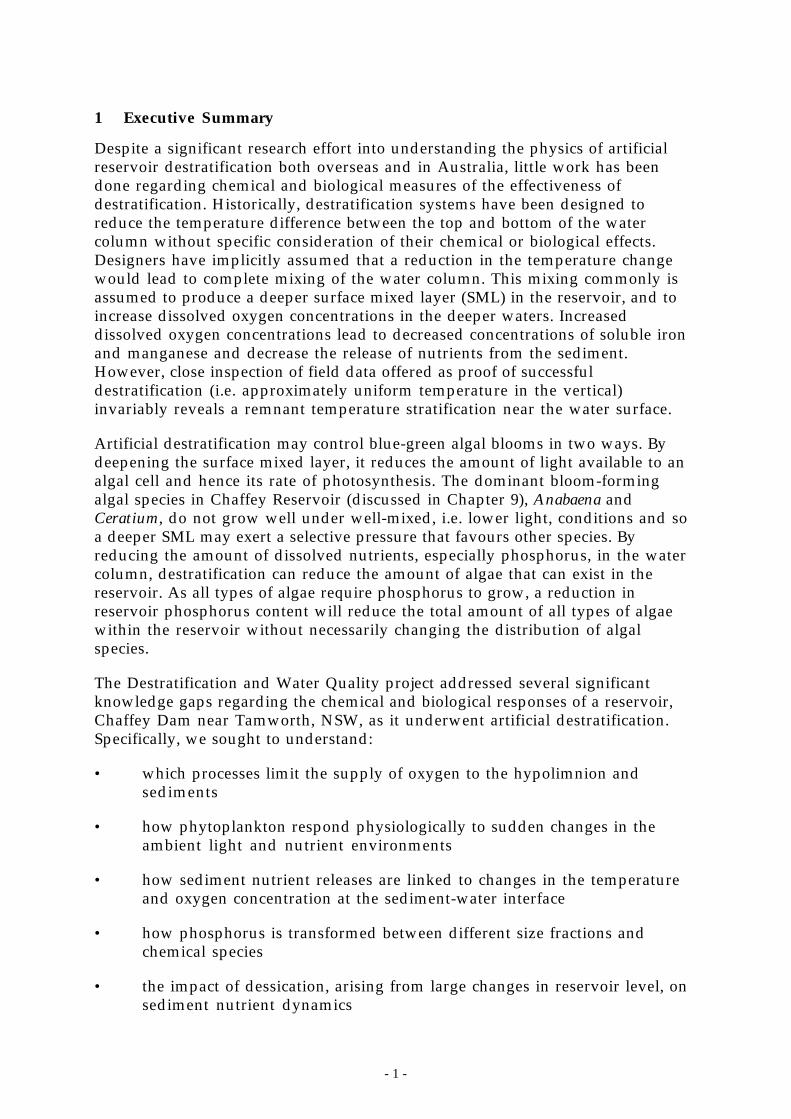
1 Executive Summary

Despite a significant research effort into understanding the physics of artificialreservoir destratification both overseas and in Australia, little work has beendone regarding chemical and biological measures of the effectiveness ofdestratification. Historically, destratification systems have been designed toreduce the temperature difference between the top and bottom of the watercolumn without specific consideration of their chemical or biological effects.Designers have implicitly assumed that a reduction in the temperature changewould lead to complete mixing of the water column. This mixing commonly isassumed to produce a deeper surface mixed layer (SML) in the reservoir, and toincrease dissolved oxygen concentrations in the deeper waters. Increaseddissolved oxygen concentrations lead to decreased concentrations of soluble ironand manganese and decrease the release of nutrients from the sediment.However, close inspection of field data offered as proof of successfuldestratification (i.e. approximately uniform temperature in the vertical)invariably reveals a remnant temperature stratification near the water surface.

Artificial destratification may control blue-green algal blooms in two ways. Bydeepening the surface mixed layer, it reduces the amount of light available to analgal cell and hence its rate of photosynthesis. The dominant bloom-formingalgal species in Chaffey Reservoir (discussed in Chapter 9), Anabaena andCeratium, do not grow well under well-mixed, i.e. lower light, conditions and soa deeper SML may exert a selective pressure that favours other species. Byreducing the amount of dissolved nutrients, especially phosphorus, in the watercolumn, destratification can reduce the amount of algae that can exist in thereservoir. As all types of algae require phosphorus to grow, a reduction inreservoir phosphorus content will reduce the total amount of all types of algaewithin the reservoir without necessarily changing the distribution of algalspecies.

The Destratification and Water Quality project addressed several significantknowledge gaps regarding the chemical and biological responses of a reservoir,Chaffey Dam near Tamworth, NSW, as it underwent artificial destratification.Specifically, we sought to understand:

• which processes limit the supply of oxygen to the hypolimnion andsediments

• how phytoplankton respond physiologically to sudden changes in theambient light and nutrient environments

• how sediment nutrient releases are linked to changes in the temperatureand oxygen concentration at the sediment-water interface

• how phosphorus is transformed between different size fractions andchemical species

• the impact of dessication, arising from large changes in reservoir level, onsediment nutrient dynamics

- 2 -

• the quantities of nutrient supplied to the reservoir from internal(sediment) and external (catchment) sources

Routine field sampling took place from September 1995 to June 1997. Thissampling program supplemented the existing monitoring performed by theNSW DLWC. Ten intensive field experiments of 7-10 days duration wereundertaken to examine short-term effects of artificial destratification. In addition,DLWC provided its entire historical water quality database for the reservoir andcatchment so that data collected by the project could be placed in a historicalcontext.

Significant findings -

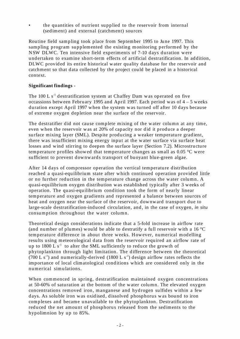
The 100 L s-1 destratification system at Chaffey Dam was operated on fiveoccassions between February 1995 and April 1997. Each period was of 4 – 5 weeksduration except April 1997 when the system was turned off after 10 days becauseof extreme oxygen depletion near the surface of the reservoir.

The destratifier did not cause complete mixing of the water column at any time,even when the reservoir was at 20% of capacity nor did it produce a deepersurface mixing layer (SML). Despite producing a weaker temperature gradient,there was insufficient mixing energy input at the water surface via surface heatlosses and wind stirring to deepen the surface layer (Section 7.2). Microstructuretemperature profiles showed that temperature changes as small as 0.05 °C weresufficient to prevent downwards transport of buoyant blue-green algae.

After 14 days of compressor operation the vertical temperature distributionreached a quasi-equilibrium state after which continued operation provided littleor no further reduction in the temperature change across the water column. Aquasi-equilibrium oxygen distribution was established typically after 3 weeks ofoperation. The quasi-equilibrium condition took the form of nearly lineartemperature and oxygen gradients and represented a balance between sources ofheat and oxygen near the surface of the reservoir, downward transport due tolarge-scale destratification-induced circulation, and, in the case of oxygen, in situconsumption throughout the water column.

Theoretical design considerations indicate that a 5-fold increase in airflow rate(and number of plumes) would be able to destratify a full reservoir with a 16 °Ctemperature difference in about three weeks. However, numerical modellingresults using meteorological data from the reservoir required an airflow rate ofup to 1800 L s-1 to alter the SML sufficiently to reduce the growth ofphytoplankton through light limitation. The difference between the theoretical(700 L s-1) and numerically-derived (1800 L s-1) design airflow rates reflects theimportance of local climatological conditions which are considered only in thenumerical simulations.

When commenced in spring, destratification maintained oxygen concentrationsat 50-60% of saturation at the bottom of the water column. The elevated oxygenconcentrations removed iron, manganese and hydrogen sulfides within a fewdays. As soluble iron was oxidised, dissolved phosphorus was bound to ironcomplexes and became unavailable to the phytoplankton. Destratificationreduced the net amount of phosphorus released from the sediments to thehypolimnion by up to 85%.

- 3 -

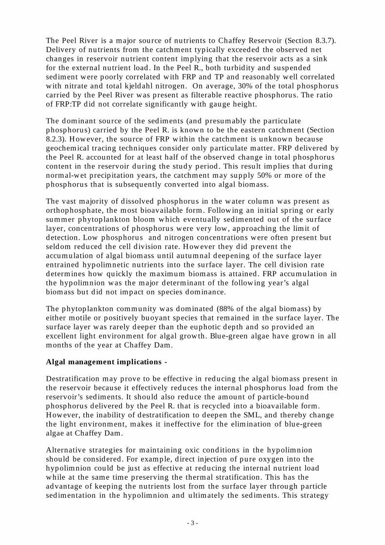
The Peel River is a major source of nutrients to Chaffey Reservoir (Section 8.3.7).Delivery of nutrients from the catchment typically exceeded the observed netchanges in reservoir nutrient content implying that the reservoir acts as a sinkfor the external nutrient load. In the Peel R., both turbidity and suspendedsediment were poorly correlated with FRP and TP and reasonably well correlatedwith nitrate and total kjeldahl nitrogen. On average, 30% of the total phosphoruscarried by the Peel River was present as filterable reactive phosphorus. The ratioof FRP:TP did not correlate significantly with gauge height.

The dominant source of the sediments (and presumably the particulatephosphorus) carried by the Peel R. is known to be the eastern catchment (Section8.2.3). However, the source of FRP within the catchment is unknown becausegeochemical tracing techniques consider only particulate matter. FRP delivered bythe Peel R. accounted for at least half of the observed change in total phosphoruscontent in the reservoir during the study period. This result implies that duringnormal-wet precipitation years, the catchment may supply 50% or more of thephosphorus that is subsequently converted into algal biomass.

The vast majority of dissolved phosphorus in the water column was present asorthophosphate, the most bioavailable form. Following an initial spring or earlysummer phytoplankton bloom which eventually sedimented out of the surfacelayer, concentrations of phosphorus were very low, approaching the limit ofdetection. Low phosphorus and nitrogen concentrations were often present butseldom reduced the cell division rate. However they did prevent theaccumulation of algal biomass until autumnal deepening of the surface layerentrained hypolimnetic nutrients into the surface layer. The cell division ratedetermines how quickly the maximum biomass is attained. FRP accumulation inthe hypolimnion was the major determinant of the following year’s algalbiomass but did not impact on species dominance.

The phytoplankton community was dominated (88% of the algal biomass) byeither motile or positively buoyant species that remained in the surface layer. Thesurface layer was rarely deeper than the euphotic depth and so provided anexcellent light environment for algal growth. Blue-green algae have grown in allmonths of the year at Chaffey Dam.

Algal management implications -

Destratification may prove to be effective in reducing the algal biomass present inthe reservoir because it effectively reduces the internal phosphorus load from thereservoir’s sediments. It should also reduce the amount of particle-boundphosphorus delivered by the Peel R. that is recycled into a bioavailable form.However, the inability of destratification to deepen the SML, and thereby changethe light environment, makes it ineffective for the elimination of blue-greenalgae at Chaffey Dam.

Alternative strategies for maintaining oxic conditions in the hypolimnionshould be considered. For example, direct injection of pure oxygen into thehypolimnion could be just as effective at reducing the internal nutrient loadwhile at the same time preserving the thermal stratification. This has theadvantage of keeping the nutrients lost from the surface layer through particlesedimentation in the hypolimnion and ultimately the sediments. This strategy

- 4 -

should produce lower algal biomass in summer and autumn than woulddestratification which resuspends some of the nutrients in the water column.

Increased emphasis on tracing catchment FRP as opposed to TP sources isrequired for informed catchment management decision making. A largeproportion of TP (30%), is delivered by the Peel River as FRP. Geochemicalsediment tracing techniques cannot identify the source of FRP within thecatchment. Unequivocal identification of the catchment FRP source(s) willrequire the deployment of streamflow guages and stage-dependent samplers onthe tributaries to the Peel upstream of Taroona in order to compute nutrientloads. An earlier attempt by DLWC to identify these sources using ‘rising stage’samplers did not provide data of sufficient quality to estimate loads.

There is insufficient Fe available to scavenge all the FRP in the water columnwhen the destratifier is operating. Operation of the destratifier converts reducediron (FeII) with a low affinity to bind phosphorus to iron oxyhydroxide (FeIIIOOH)which has a high phosphorus binding affinity. The imbalance between Fe andFRP increases the importance of controlling FRP delivery from the catchment.Manganese is often present in higher concentrations than Fe in the anoxichypolimnion but it does not play a significant role in P reduction.

Dessication of dam sediments decreased the capacity of sediments to both take upP, and to release P under anoxic conditions. The duration of this effect isunknown but is believed to depend on the time required for the anaerobicbacteria to recolonize the sediment following reinundation. It may be possible toreduce the internal P load by operating the dam to cause low water levels ofsufficient duration to dessicate a significant portion of the sediments.

Extensive sulphate reduction occurs during summer stratification and thiscontributes a significant portion of the internal phosphorus load. Maintenance ofaerobic conditions within the hypolimnion may prevent sulphate reduction andthe attendant release of phosphorus.

Elbow-grab water samples gave higher biomass estimates than 5 m-integratedsamples, especially during periods of blue-green algal dominance. Werecommend the pooling of 5 m-integrated samples from 5 locations in thereservoir into a single sample for algal abundance estimates. This will provide amore representative estimate of reservoir conditions. However, if contact withalgal scums is an issue, then surface samples need to be collected as well.

- 5 -

2 Glossary of terms

Abiotic - A process that does not require the action of living organisms, Non-biological e.g. a chemical reaction.

Absorption cross section – The area of the pigment molecules within an algal cellused to intercept light.

Adsorption - ‘sticking’ of chemical compounds to surfaces. Adsorption can eitherbe by physical adsorption, when the chemical is held to the surface by somephysical force (e.g. ionic attraction), or chemical adsorption where the adsorbedsubstance forms one or more chemical bonds with the surface.

Algal Blooms - excessive number of algae in a water body. Often, but notnecessarily always, associated with nutrient pollution. As a rule-of-thumb, achlorophyll concentration of greater than 20 µg per litre (0.00002 g per litre) isconsidered an algal bloom.

Ammonia - a gas with the chemical formulae NH3

Anoxic - the absence of oxygen. Often used interchangeably with anaerobic whichmeans in the absence of air.

Artificial destratification – The process of reducing the temperature differencebetween the bottom and top of the water column by increasing the verticalcirculation of water. This is typically done by injecting compressed air in thedeepest part of a reservoir (bubble-plume destratification, often called reservoiraeration), but can also be accomplished by the use of impellers (sometimes calledsurface pumps).

Assimilated - taken into an organism and used to produce biomass.

Base - a base is a substance which reacts with the hydrogen ion H+. The oppositeto base is acid. An acid is a substance which can release a hydrogen ion. See alsoproton.

Bioavailable - A description of how easily a compound can be assimilated by anorganism.

Biodiversity - or species diversity. A measure of the number of plants andanimal species present in an ecosystem. Eutrophic systems tend to have a largebiomass but low biodiversity

Biofilm - thin layers of mixed groups of micro-organisms that coat submergedsurfaces. The structure of biofilms can be quite complex and can contain both oxicand anoxic zones even though the water surrounding the biofilm is welloxygenated

Biomass - The weight of all the organisms in an ecosystem, trophic level etc.

- 6 -

Biota - a term used to describe all the organisms in an ecosystem. e.g. freshwaterbiota.

Chlorophyll - a green pigment found in most plants and algae. It is used tocapture light in photosynthesis.

Colloids - small particles usually less than about 0.0001 mm across which aresuspended in solution. They may be made of minerals, clays or organiccompounds. They are important in adsorption in many freshwater systems.

Coupled nitrification-denitrification - process for the biological conversion ofammonia to nitrogen gas. Occurs where oxic and anoxic zones are close together.

Cyanobacteria – Also called blue-green algae. These photosynthetic bacteria arethe main nuisance species present in Chaffey Reservoir due to their occassionalrelease of toxins to the water.

Decomposition - decay of biomass usually into more simple compounds bymicro-organisms. The process consumes oxygen and often has ammonia as a by-product - see also mineralisation.

Dinoflagellate – A type of phytoplankton that possess flagellae which allows it toswim within the water column under calm conditions.

Denitrification - process where nitrate is converted to nitrogen gas. Occurs underanoxic conditions. The process is mediated by bacteria.

Dissimilatory Nitrate Reduction to Ammonia - process where nitrate isconverted to ammonia. This process occurs in the anoxic zone of sediments

Downwelling – Moving vertically downwards from the sky to the water.

Electron acceptor - The oxidant used in the oxidation of organic matter duringrespiration. For example under oxic conditions, an organism takes up oxygen..The oxygen is used to oxidise carbon. Because the oxygen accepts electrons fromthe carbon molecules the oxygen molecules are said to be reduced (see reduction).Oxygen therefore is an electron acceptor. Where oxygen is unavailable (e.g. inanoxic zones), bacteria use other electron acceptors - e.g. ferric iron in ironreduction and sulfate in sulfate reduction.

Eutrophic - containing abundant nutrients - see eutrophication.

Eutrophication - process where excessive amounts of nutrients, usually N and P,are added to water bodies. Usually results in increased plant and algal biomassbut decreased biodiversity.

External nutrient load – The supply of nutrients to the water column that isdelivered to the reservoir from sources outside the high water level of thereservoir. Usually dominated by sediment and dissolved nutrients from sourceswithin the catchment upstream.

- 7 -

Ferric iron - Oxidised form of iron. Stable in air. Has 3 positive charges - Fe3+.Often in the form of solid iron oxides such as haematite.

Ferrous iron - Reduced form of iron. Iron compounds having a 2 positive charge- Fe2+. Ferrous compounds are unstable in the presence of oxygen and are quicklyoxidised to ferric compounds.

Filterable reactive phosphorus (FRP) – The amount of inorganic and organicphosphorus compounds dissolved in a water sample. The inorganic componentis typically regarded as being immediately available to fuel algal growth.

Fluorescence – The portion of the energy absorbed by a substance exposed to anexcitation light source which is reemited as light at a longer wavelength. Theenergy of a photon decreases as the wavelength increases so the shift to a longerwavelength reflects losses of the absorbed light energy (e.g. As heat or conversionto chemical energy) prior to reemission as fluorescence.

Food Chain - Chain of organisms through which energy, in the form of carbon,progresses. A simple food-chain consists of producers (plants), which convert theenergy in sunlight into chemical compounds (biomass). Plants are inturn eatenby smaller animals (1st order consumers or herbivores ) which are then eaten byhigher order consumers (carnivores).

Hypolimnion – The lowest part of the water column. It extends from thesediments to the bottom of the thermocline.

Internal nutrient load – The supply of nutrients to the water column thatoriginates from within the reservoir. Usually, the reservoir sediments are thedominant source.

Ion - an electrically charged atom or molecule. Compounds with a positivecharge are called cations, compounds with a negative charge are called anions.

Iron-Reducing Bacteria - group of bacteria which reduce ferric iron to ferrous ironin anaerobic respiration.

Isotopes of oxygen, nitrogen, and carbon – Used to infer the source and age ofnutrients assimilated by algal cells.

Longwave radiation – Infrared radiation emitted mainly from water vapour inthe atmosphere.

Microstructure – Changes in the thermal or chemical structure of a reservoir thatoccur over very small distances of the order of a centimetre or less.dissolvedinorganic nitrogen – The amount of inorganic nitrogen compounds dissolved ina water sample and available to fuel algal growth. Typically assumed to beammonia plus nitrite plus nitrate.

Mineralisation - conversion of nitrogen in biomass to ammonia -seeDecomposition.

- 8 -

Nitrate - oxidised form of nitrogen with the formulae NO3-. Can be assimilated by

plants including algae.

Nitrification - process where ammonia is converted to nitrate. Usually goesthrough two steps. NH3 is first converted to nitrite (NO2

-) which is thenconverted to nitrate. Nitrification requires oxygen.

Nitrite - NO2- ion.

Nitrogenase - the enzyme responsible for nitrogen fixation.

Nitrogen Fixation - the process where atmospheric nitrogen (N2) is converted toammonia. Nitrogen fixation is an important pathway for N to enter bothterrestrial and aquatic ecosystems.

Nucleic acids - large molecules containing N and P occurring in all livingorganisms. Nucleic acids are used to store and transfer the genetic make-up ofthe organism. DNA and RNA.

Organic Phosphorus - Chemical compounds which contain both phosphorus andcarbon atoms. They usually contain a C-O-P bond (phosphate esters) butcompounds containing a direct C-P bond (phosphonates) are also known to occurnaturally. To become bioavailable to algae organic P compounds need to bebroken down.

Ortho-phosphate - HxPO4(3-x)-. The only form of phosphate that can cross bacterial

or algal cell membranes, therefore, the most bioavailable form of P.

Oxic - Contains oxygen. The opposite of anoxic.

Oxidation - Chemical process where a molecule loses an electron and thereforeloses some negative electrical charge or gains some positive charge e.g.S2- -> S + 2e- orFe2+ -> Fe3+ + e-

It is almost always coupled with reduction reaction.

Photophysiology – The processes within an algal cell responsible for theconversion of light energy into chemical energy. This includes everything fromthe pigments such as chlorophyll-a used to capture light energy (photons) to themany chemical compounds used to process the captured energy.

Photosynthesis - process where energy from sunlight is used to make chemicalcompounds. These compounds are a form of energy which can be used in foodchains.

pKa - the pH at which half of a compound is in it’s protonated form and half inits basic form.

Prokaryotic - organisms whose DNA is not separated from the rest of the cell by amembrane. Includes both bacteria and blue-green algae (cyanobacteria).

- 9 -

Proteins - large molecules which contain nitrogen. Proteins are essential forliving organisms. Enzymes are a type of protein.

Proton - The hydrogen ion H+. The concentration of protons determines the pHof a solution

Protonated - gaining a proton.

Polymer - Large molecules which consist of one or more molecules joined to eachother in a repetitive sequence.

Polyphosphate -polymer of orthophosphate ions such as tripolyphosphate.

Quantum yield – A measure of the efficiency with which captured photons areconverted to chemical energy within an algal cell.

Reduction - chemical process where a molecule gains an electron - the converseof oxidation.

Respiration - The process where an organism gains energy from the oxidation ofcarbon compounds (such as sugars).

Secchi depth – The maximum depth under the water at which a white & blackdisk can be seen by an observer immediately above the water surface.

Sediment - The complex mixture of minerals, clays, organic material and biotafound at the bottom of waterbodies. Varies in consistency from corse sands andgravels to very fine mud. Fine sediments often have an anoxic zone.

Sediment trap – A device that collects particles that move through the watercolumn. Upwards facing traps collect sinking particles whereas downwards facingtraps collect rising particles.

Shortwave radiation – Visible light from the sun.

Stratification – The presence of a changing temperature distribution within thewater of a reservoir. Typically refers to the presence of warm water at the surfaceand colder water at the bottom of the water column.

Sulfate- oxidised form of sulfur - SO42-

Sulfate-reducing bacteria - group of bacteria which reduce sulfate to sulfide inanaerobic respiration.

Sulfide - reduced form of sulfur S2- ion. When protonated it forms H2S - rotten

egg gas.

Surface mixed layer (SML)– The uppermost region of the water column that iswell-mixed. Temperature, algal and chemical concentrations are uniform withinthe SML. Its depth varies continuously throughout the day.

- 10 -

Thermocline – The vertical portion of the water column with the greatesttemperature change across it. At Chaffey Reservoir it typically extends from 4 or 5m below the surface to approximately 12 m below the surface.

Total nitrogen (TN) – The total amount of nitrogen present in a water samplefrom all sources, i.e. Dissolved plus particulate.

Total phosphorus (TP) – The total amount of phosphorus present in a watersample from all sources, i.e. Dissolved plus particulate.

Tripolyphosphate - a polymer of phosphate groups used in detergents todecrease the hardness of water.

Turbulent velocity scale – The characteristic speed of parcels of water as theymove about a turbulent region of the water column. The technology to directlymeasure the turbulent velocity scale is relatively new. It’s value is more typicallyinferred from measurements of other more easily measured parameters, typicallyheat flux and wind speed.

Upwelling – Moving vertically upwards, e.g. from the water to the sky.

- 11 -

3 Introduction

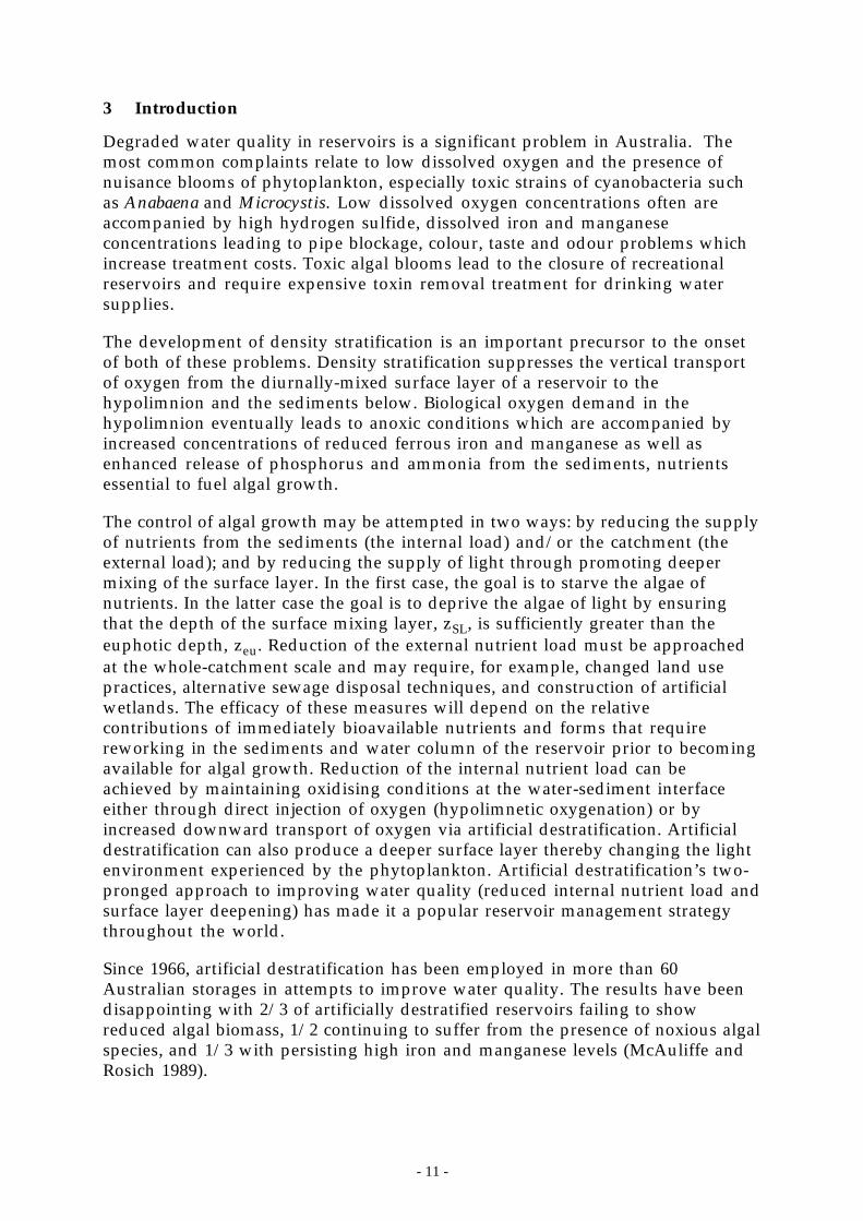
Degraded water quality in reservoirs is a significant problem in Australia. Themost common complaints relate to low dissolved oxygen and the presence ofnuisance blooms of phytoplankton, especially toxic strains of cyanobacteria suchas Anabaena and Microcystis. Low dissolved oxygen concentrations often areaccompanied by high hydrogen sulfide, dissolved iron and manganeseconcentrations leading to pipe blockage, colour, taste and odour problems whichincrease treatment costs. Toxic algal blooms lead to the closure of recreationalreservoirs and require expensive toxin removal treatment for drinking watersupplies.

The development of density stratification is an important precursor to the onsetof both of these problems. Density stratification suppresses the vertical transportof oxygen from the diurnally-mixed surface layer of a reservoir to thehypolimnion and the sediments below. Biological oxygen demand in thehypolimnion eventually leads to anoxic conditions which are accompanied byincreased concentrations of reduced ferrous iron and manganese as well asenhanced release of phosphorus and ammonia from the sediments, nutrientsessential to fuel algal growth.

The control of algal growth may be attempted in two ways: by reducing the supplyof nutrients from the sediments (the internal load) and/or the catchment (theexternal load); and by reducing the supply of light through promoting deepermixing of the surface layer. In the first case, the goal is to starve the algae ofnutrients. In the latter case the goal is to deprive the algae of light by ensuringthat the depth of the surface mixing layer, zSL, is sufficiently greater than theeuphotic depth, zeu. Reduction of the external nutrient load must be approachedat the whole-catchment scale and may require, for example, changed land usepractices, alternative sewage disposal techniques, and construction of artificialwetlands. The efficacy of these measures will depend on the relativecontributions of immediately bioavailable nutrients and forms that requirereworking in the sediments and water column of the reservoir prior to becomingavailable for algal growth. Reduction of the internal nutrient load can beachieved by maintaining oxidising conditions at the water-sediment interfaceeither through direct injection of oxygen (hypolimnetic oxygenation) or byincreased downward transport of oxygen via artificial destratification. Artificialdestratification can also produce a deeper surface layer thereby changing the lightenvironment experienced by the phytoplankton. Artificial destratification’s two-pronged approach to improving water quality (reduced internal nutrient load andsurface layer deepening) has made it a popular reservoir management strategythroughout the world.

Since 1966, artificial destratification has been employed in more than 60Australian storages in attempts to improve water quality. The results have beendisappointing with 2/3 of artificially destratified reservoirs failing to showreduced algal biomass, 1/2 continuing to suffer from the presence of noxious algalspecies, and 1/3 with persisting high iron and manganese levels (McAuliffe andRosich 1989).

- 12 -

This report presents the results of a 3-year study by the Cooperative ResearchCentre for Freshwater Ecology into the coupling between the physical, chemicaland biological processes within Chaffey Reservoir that exert the greatest influenceon the water column chemistry and the phytoplankton community. Theultimate objective of the study was to identify the intrinsic limitations of artificialdestratification and to be able to provide sound advice to the NSW Dept. of Landand Water Conservation (DLWC), the Chaffey Dam Advisory Committee(CDAC), the National Eutrophication Management Program (NEMP), and theAustralian water industry on the most effective management strategies for thecontrol of cyanobacteria and the transport of oxygen to the hypolimnion.

From conception there has been a whole-ecosystem approach to the experimentaldesign of the project. To do this it was necessary to study the physiologicalresponses of the phytoplankton to changes in nutrient status and the lightenvironment to identify the factors that controlled the growth of bothindividuals as well as the community as a whole. It was also necessary to studythe sinks for the algae such as zooplankton grazing and sedimentation out of theeuphotic zone. Detailed hydrodynamic and meteorological data were required toidentify the major processes influencing the light and chemical conditions thatconfer competitive advantages to different phytoplankton species. Withoutnutrients there could be no algae so the major sources and sinks of nutrients hadto be identified and the transformations between different chemical speciesconsidered. This meant that nutrient sources both external, i.e. the Peel River,and internal, especially the sediments, had to be quantified.

A complementary motivation was the desire to collect the most comprehensivedata set yet available to rigorously test complex reservoir water quality modelswhich for decades have encapsulated contemporary understanding of nutrientpathways and trophic dynamics - the conceptual models of reservoir ecologyhaven’t changed significantly in 20 years - but have never been thoroughlyvalidated. The vast number of processes and parameters in these models requireextensive calibration and may produce plausible results for the wrong reasons;e.g. the presence of compensating errors is likely but often escapes detectionbecause the relevant field data aren’t available. Constraining these models bymeasuring the important rate coefficients, forcing parameters, etc. makes itpossible to identify shortcomings in the models and to evaluate the significanceof modelled processes for which field data are not easily obtained.

3.1 Why Chaffey Reservoir?

Chaffey Reservoir, near Tamworth in NSW, is an example of a storage wheredestratification has failed to live up to expectations. Despite the reduction indensity stratification and the increased dissolved oxygen levels at depth producedby artificial destratification, the reservoir still suffered from massive blooms ofthe toxic cyanobacteria, Anabaena and Microcystis, which could occur at virtuallyany time of year.

Chaffey Reservoir was selected because it offered the best combination ofattributes for such a large study. It’s long history of algal bloom problems had ledto a number of studies being carried out in the reservoir and the catchmentupstream. There was a long and continuous historical data record that includedalgal abundance and vertical profiles of water column chemistry at weekly to

- 13 -

fortnightly intervals. An automated water quality sampler was available a fewkilometres upstream of the dam so that the external nutrient load could bequantified. A compressed-air destratification system was available on-site whichDLWC was willing to operate solely to comply with the research objectives of thisproject. There was also strong support for the project from the local community.

The outstanding data set compiled by this project owes much of its existence tothe tireless support of the DLWC staff at Chaffey Dam. They maintainedinstruments for us, collected samples whenever asked, and made us feel verywelcome every time we dropped in for a field experiment.

- 15 -

4 Site description

4.1 Location

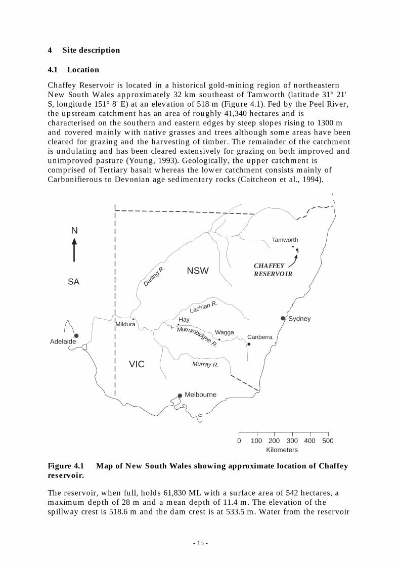
Chaffey Reservoir is located in a historical gold-mining region of northeasternNew South Wales approximately 32 km southeast of Tamworth (latitude 31° 21'S, longitude 151° 8' E) at an elevation of 518 m (Figure 4.1). Fed by the Peel River,the upstream catchment has an area of roughly 41,340 hectares and ischaracterised on the southern and eastern edges by steep slopes rising to 1300 mand covered mainly with native grasses and trees although some areas have beencleared for grazing and the harvesting of timber. The remainder of the catchmentis undulating and has been cleared extensively for grazing on both improved andunimproved pasture (Young, 1993). Geologically, the upper catchment iscomprised of Tertiary basalt whereas the lower catchment consists mainly ofCarbonifierous to Devonian age sedimentary rocks (Caitcheon et al., 1994).

Adelaide

Melbourne

SydneyMildura

Hay

WaggaCanberra

Darlin

g R.

Lachlan R.

Murray R.

Kilometers

N

SANSW

0 100 200 300 400 500

CHAFFEYRESERVOIR

VIC

Tamworth

Murrumbidgee R.

Figure 4.1 Map of New South Wales showing approximate location of Chaffeyreservoir.

The reservoir, when full, holds 61,830 ML with a surface area of 542 hectares, amaximum depth of 28 m and a mean depth of 11.4 m. The elevation of thespillway crest is 518.6 m and the dam crest is at 533.5 m. Water from the reservoir

- 16 -

is used both for irrigation and to supplement the drinking water supply for thecity of Tamworth, one of the largest cities in rural New South Wales.

The reservoir has a history of chronic algal blooms and is notable because toxicblooms of both Microcystis sp. and Anabaena sp. can occur at virtually any time ofyear with dense blooms often occurring during the winter months (see Chapter7). This has motivated an unusually intensive routine data acquisition programby the dam’s operator, DLWC. A number of field studies have also taken placeover the years since the reservoir was first inundated in 1979 and cover a range oftopics from catchment geology and phosphorus sources (Caitcheon et al. 1994,Beecham, 1995) to the biota of the Peel River and Chaffey Reservoir (May andPowell, 1986; Muschal, 1995). The issue of phosphorus sources has beenparticularly contentious with some arguing that the basaltic geology of the uppercatchment is primarily responsible for the external phosphorus load (Donnelly,1993; Caitcheon et al., 1994) while others assert that runoff from fertilised pasturesare the dominant source of P (Beecham, 1995). As will be shown in Chapter 5,neither argument can be dismissed.

4.2 Facilities

4.2.1 Historical data archive

The NSW DLWC provided files containing virtually all of the historical data theyhad compiled from previous studies and routine monitoring at Chaffey Dam.The large number of fragmented and occasionally overlapping files wereconsolidated, checked for obvious errors, converted into a standard database fileformat (dBASE, .dbf) and made available to all project partners via ftp from thefileserver at CSIRO Land & Water. Historical data included Peel River inflowvolumes, reservoir level and discharge values, compressor operating times, algalcount data, and water chemistry data.

4.2.2 Destratification system

Since its inception, Chaffey Reservoir has had a compressed-air, bubble-plumedestratification system. The initial system consisted of 3 diffusers anchored inconcrete blocks about 100 m from the dam wall (Young, 1993). The compressorhad a maximum free airflow rate of 100 L s-1. In 1988, one of the airlines failed andthe system was mothballed until the current project commenced because it wasfelt that the system hadn’t performed satisfactorily.

The destratification system was redesigned for the current experiment followingthe design criteria described by Schladow (1993) and Lemckert et al. (1993). Thesecriteria are based on research into the dynamics of bubble plumes (McDougall,1978; Asaeda and Imberger, 1993) and identify the optimal configuration of abubble plume to maximise the efficiency of a destratification system whereefficiency is defined as the increase in potential energy1 of the water columndivided by the energy consumed by the compressor.

1 The potential energy of a water column is defined as its mass times gravitational accelerationtimes the difference in height between the centre of masses of the stratified water column and awell-mixed water column of the same mass. A well-mixed water column has a higher centre of mass

- 17 -

0

5

10

15

20

25

Temperature (°C)

Dep

th (

m)

10 15 20 25 30

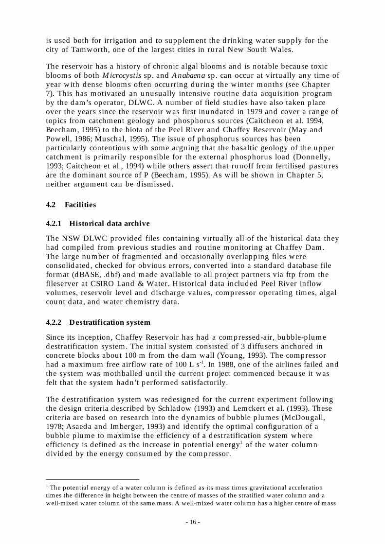
Figure 4.2 Temperature profile at Chaffey Reservoir on 2 Feb 1993.

The design objective for the new bubble plume system was that it should be ableto destratify the maximum stratification observed in the reservoir under thetypical summer meterological conditions, i.e. strong insolation, high airtemperature and light winds. To facilitate testing of the intermediate disturbancehypothesis – one of the project’s initial goals – complete destratification shouldoccur within one week so that rapid, profound changes in the underwater lightclimate (i.e. zSL:zeu) on phytoplankton physiology could be assessed. This 7 daytime scale for destratification is much more stringent than the 21 days consideredacceptable for normal reservoir operation (Schladow, 1993).

The design temperature profile is shown in Figure 4.2. This profile is typical ofsummer conditions in the reservoir. When the reservoir level decreases, thehypolimnion becomes shallower whereas the surface layer and thermoclineregions generally maintain the same dimensions. The temperature profile indeeper water columns was approximated by extrapolating the hypolimneticprofile downwards to the relevant depth.

For water depths between 22 and 28 m – the expected range of reservoir level forthe project – the potential energy of the stratification in Figure 4.2 is equivalent toa linear temperature gradient of 0.62-0.59 °C m-1 which gives a buoyancyfrequency range of 0.033-0.026 s-1. The results of the design calculations are shownin Table 4.1. Also shown in the table are the results for the minimum watercolumn depth during the project. For details regarding the derivation of theparameters in the table the reader is referred to the original articles by Schladow(1993) and Lemckert et al. (1993). The most energy efficient design for a bubble

and therefore a higher potential energy than a stratified water column because the density of astratified water column is greater at the bottom than at the top.

- 18 -

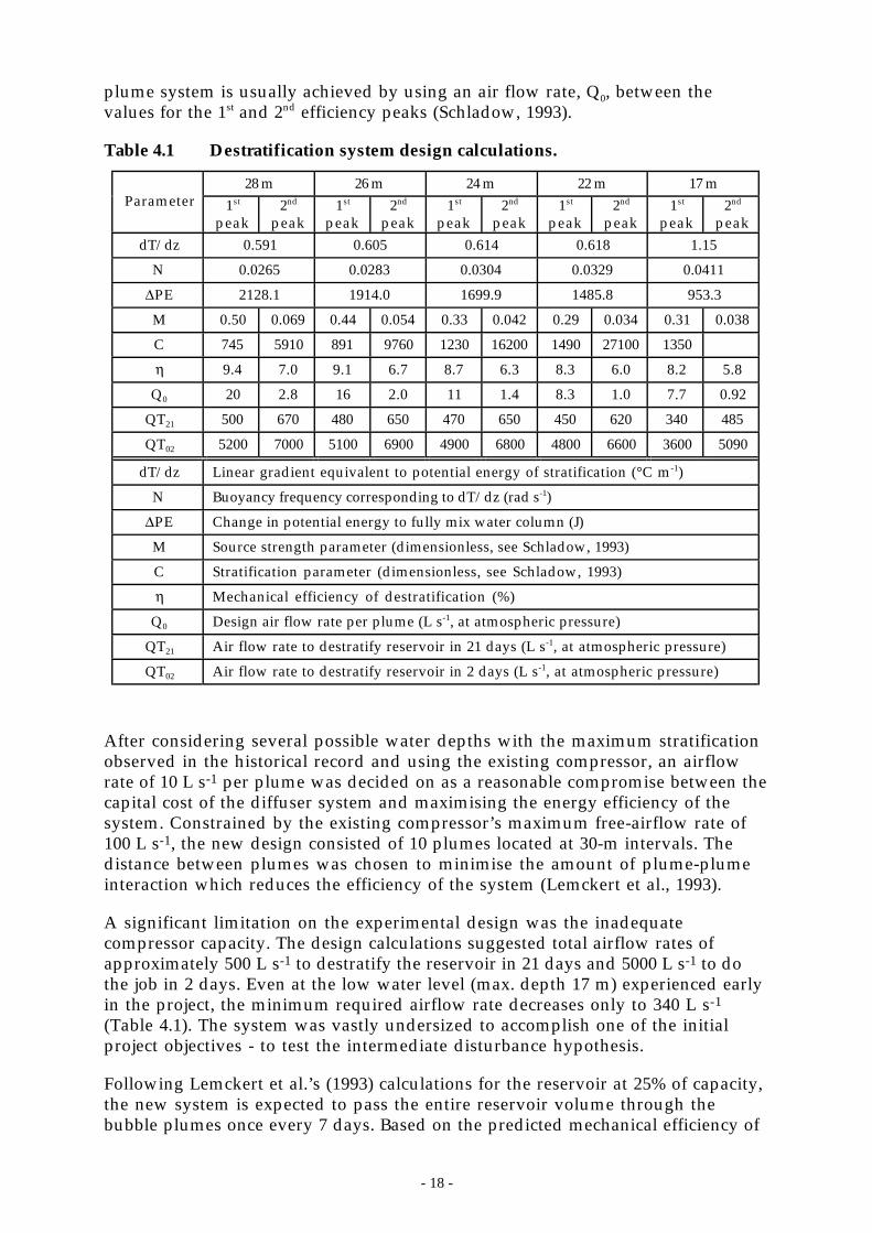
plume system is usually achieved by using an air flow rate, Q0, between thevalues for the 1st and 2nd efficiency peaks (Schladow, 1993).

Table 4.1 Destratification system design calculations.

28 m 26 m 24 m 22 m 17 mParameter 1st

peak2nd

peak1st

peak2nd

peak1st

peak2nd

peak1st

peak2nd

peak1st

peak2nd

peakdT/dz 0.591 0.605 0.614 0.618 1.15

N 0.0265 0.0283 0.0304 0.0329 0.0411

∆PE 2128.1 1914.0 1699.9 1485.8 953.3

M 0.50 0.069 0.44 0.054 0.33 0.042 0.29 0.034 0.31 0.038

C 745 5910 891 9760 1230 16200 1490 27100 1350

η 9.4 7.0 9.1 6.7 8.7 6.3 8.3 6.0 8.2 5.8

Q0 20 2.8 16 2.0 11 1.4 8.3 1.0 7.7 0.92

QT21 500 670 480 650 470 650 450 620 340 485

QT02 5200 7000 5100 6900 4900 6800 4800 6600 3600 5090

dT/dz Linear gradient equivalent to potential energy of stratification (°C m-1)

N Buoyancy frequency corresponding to dT/dz (rad s-1)

∆PE Change in potential energy to fully mix water column (J)

M Source strength parameter (dimensionless, see Schladow, 1993)

C Stratification parameter (dimensionless, see Schladow, 1993)

η Mechanical efficiency of destratification (%)

Q0 Design air flow rate per plume (L s-1, at atmospheric pressure)

QT21 Air flow rate to destratify reservoir in 21 days (L s-1, at atmospheric pressure)

QT02 Air flow rate to destratify reservoir in 2 days (L s-1, at atmospheric pressure)

After considering several possible water depths with the maximum stratificationobserved in the historical record and using the existing compressor, an airflowrate of 10 L s-1 per plume was decided on as a reasonable compromise between thecapital cost of the diffuser system and maximising the energy efficiency of thesystem. Constrained by the existing compressor’s maximum free-airflow rate of100 L s-1, the new design consisted of 10 plumes located at 30-m intervals. Thedistance between plumes was chosen to minimise the amount of plume-plumeinteraction which reduces the efficiency of the system (Lemckert et al., 1993).

A significant limitation on the experimental design was the inadequatecompressor capacity. The design calculations suggested total airflow rates ofapproximately 500 L s-1 to destratify the reservoir in 21 days and 5000 L s-1 to dothe job in 2 days. Even at the low water level (max. depth 17 m) experienced earlyin the project, the minimum required airflow rate decreases only to 340 L s-1

(Table 4.1). The system was vastly undersized to accomplish one of the initialproject objectives - to test the intermediate disturbance hypothesis.

Following Lemckert et al.’s (1993) calculations for the reservoir at 25% of capacity,the new system is expected to pass the entire reservoir volume through thebubble plumes once every 7 days. Based on the predicted mechanical efficiency of

- 19 -

the system (Schladow, 1993), it would be expected to take 2 months to destratifythe reservoir completely during the summer under such a low volumecondition.

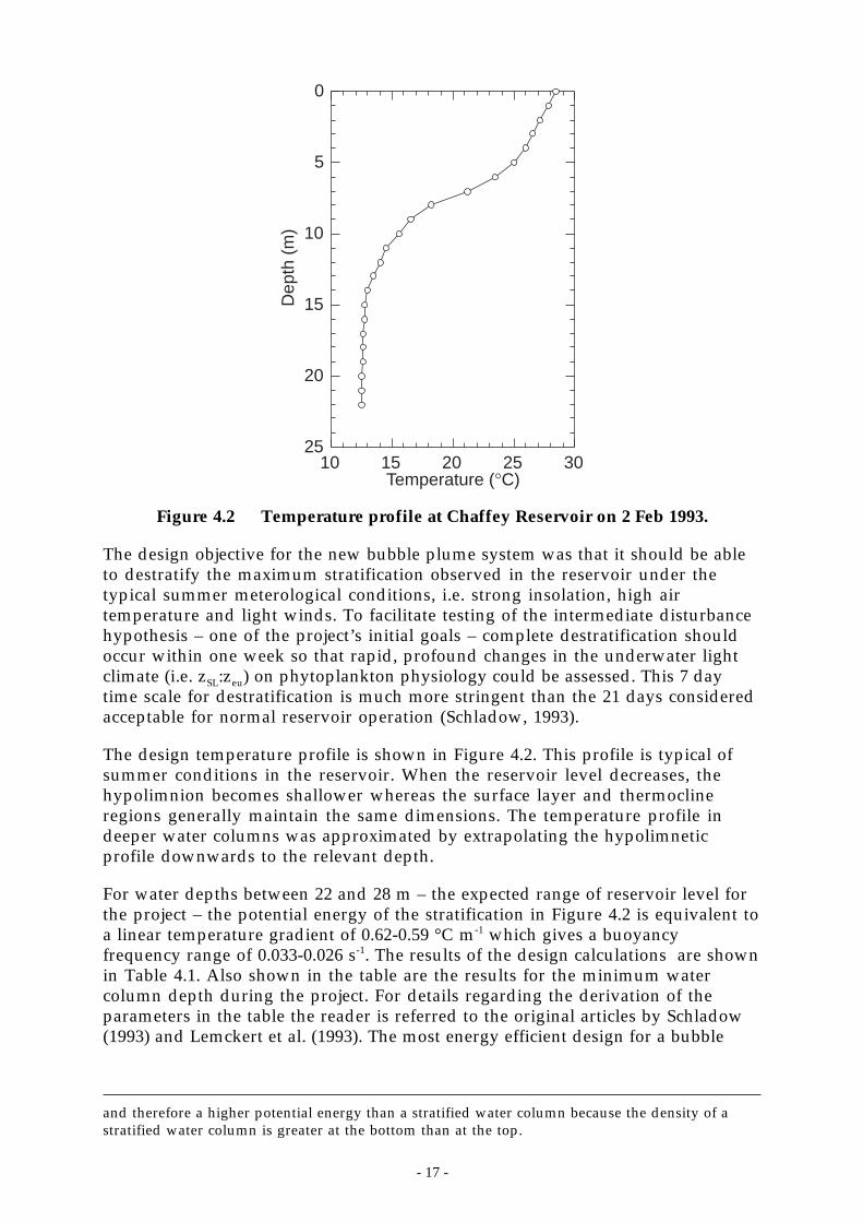
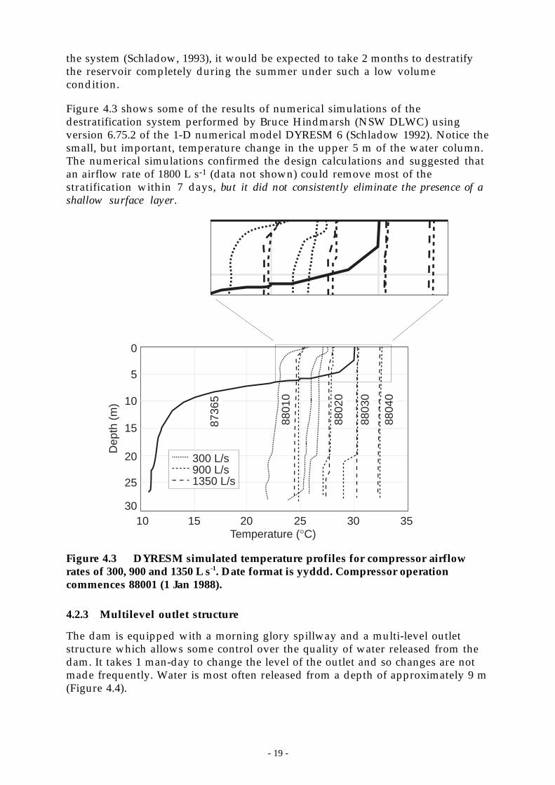
Figure 4.3 shows some of the results of numerical simulations of thedestratification system performed by Bruce Hindmarsh (NSW DLWC) usingversion 6.75.2 of the 1-D numerical model DYRESM 6 (Schladow 1992). Notice thesmall, but important, temperature change in the upper 5 m of the water column.The numerical simulations confirmed the design calculations and suggested thatan airflow rate of 1800 L s-1 (data not shown) could remove most of thestratification within 7 days, but it did not consistently eliminate the presence of ashallow surface layer.

8802

0

8801

0

8736

5

8803

0

8804

0

300 L/s

1350 L/s900 L/s

10 15 20 25 30

5

10

15

20

25

30

Dep

th (

m)

Temperature (°C)

0

35

Figure 4.3 DYRESM simulated temperature profiles for compressor airflowrates of 300, 900 and 1350 L s-1. Date format is yyddd. Compressor operationcommences 88001 (1 Jan 1988).

4.2.3 Multilevel outlet structure

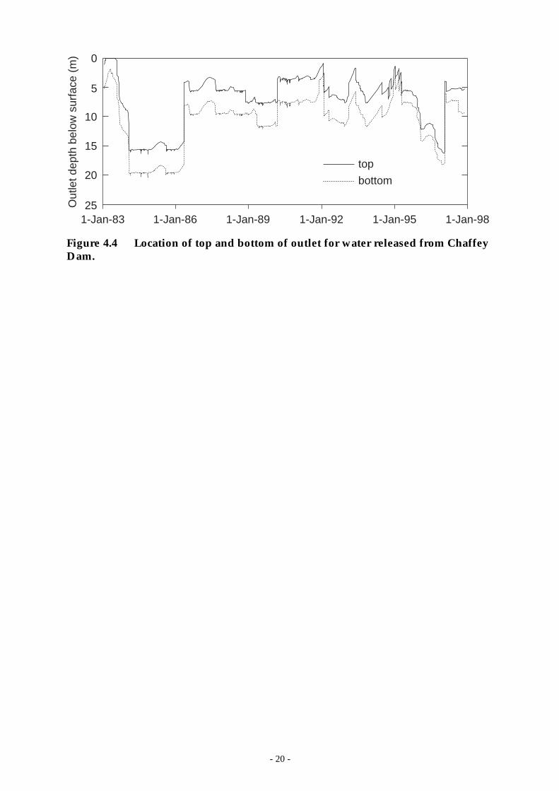
The dam is equipped with a morning glory spillway and a multi-level outletstructure which allows some control over the quality of water released from thedam. It takes 1 man-day to change the level of the outlet and so changes are notmade frequently. Water is most often released from a depth of approximately 9 m(Figure 4.4).

- 20 -

0

5

10

15

20

251-Jan-83 1-Jan-86 1-Jan-89 1-Jan-92 1-Jan-95 1-Jan-98

Out

let d

epth

bel

ow s

urfa

ce (

m)

top

bottom

Figure 4.4 Location of top and bottom of outlet for water released from ChaffeyDam.

- 21 -

5 Methods

5.1 Routine monitoring program

The routine monitoring program consisted of: meteorological and thermistorchain data gathered every 10 minutes (CRCFE); weekly conductivity-temperature-depth-dissolved oxygen (CTDO) profiles at 5 - 6 sites (depending on water level)(DLWC); weekly to fortnightly water column sampling for chemical analyses(DLWC); weekly 5 m-integrated samples at five sites analyzed for chl-a and algalabundance (CRCFE); weekly 10 m-integrated samples for zooplankton abundance(CRCFE); weekly surface grabs for algal abundance (DLWC); fortnightly tomonthly depth profiles of chemistry (CRCFE); stage-dependent sampling of thePeel River 6.7 km upstream of the reservoir at Taroona (DLWC-CRCFE); andriver flow, height, temperature, turbidity, and conductivity every 15 min(DLWC). In addition, there was a Hobo-brand temperature logger continuouslyrecording the Peel River temperature immediately upstream of the reservoir(when full). Table 5.1 shows details of the routine sampling program includinginstrumentation, measurement accuracy and frequency. The full samplingprogram commenced in September 1995 and continued uninterrupted throughJune 1997 except for a few periods when the meteorological station andthermistor chains were being serviced.

The locations of the sampling sites and the bathymetry of the reservoir are shownin Figure 5.1. The 518 m contour is the water level at 95% of capacity. During thecourse of the project the water level rose from a minimum of 506.6 m (20% cap.)during spring 1995 to 510.3 m (38% cap.) by 9 Jan 1996 with the reservoirultimately spilling on 16 Feb 1997 when the water level reached 518.72 m.

5.2 Intensive sampling program

In addition to the routine monitoring, there were 10 field trips each of 7- 10 daysduration during which intensive sampling of the reservoir’s thermal, chemicaland biological structure was undertaken. Temperature, depth, fluorescence,dissolved oxygen (TDFO) profiles were taken at 20-50 locations throughout thereservoir, often twice a day. The locations of the profiles was determined in thefield and based on the properties of the water column at the time; the distancebetween profiles decreased when strong gradients or unusual features weredetected. On two occasions, an acoustic doppler velocimeter (ADV) was used atsites TC1 and 12 to measure the water velocity profile when the destratifier wasoperated.

Depth profiles of detailed water chemistry (especially particle size fractions,phosphorus speciation and redox properties), were taken primarily at Stn 1(Figure 5.1). Sediment traps were deployed here as well. Depth profiles of algalphotophysiologal properties were taken mainly at TC1. Bottle experiments onraw water samples were deployed at A3 and TC1. Over 60 sediment samples werecollected throughout the reservoir (within the 510 m contour) for xrayfluorescence (XRF) analysis of their elemental composition, sediment particle sizeand organic carbon. Benthic chambers and peepers were deployed at severallocations to quantify the sediment oxygen demand and the fluxes of nutrientsfrom the sediments to the water column.

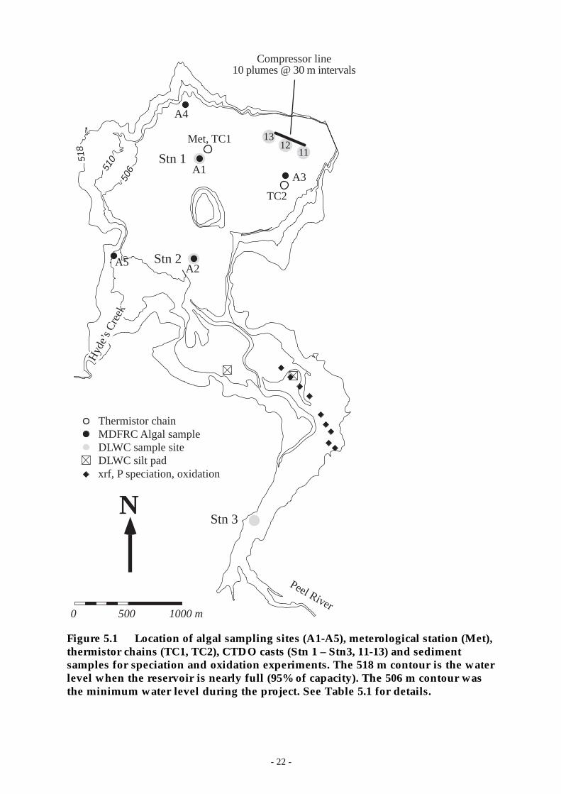
- 22 -

Met, TC1

TC2

A1

A2

A3

A4

A5

Stn 1

Stn 2

Stn 3

Compressor line10 plumes @ 30 m intervals

1312

11

Thermistor chainMDFRC Algal sampleDLWC sample site

xrf, P speciation, oxidationDLWC silt pad

N

0 500 1000 m

51051

8

506

Peel River

Hyd

e’s C

reek

Figure 5.1 Location of algal sampling sites (A1-A5), meterological station (Met),thermistor chains (TC1, TC2), CTDO casts (Stn 1 – Stn3, 11-13) and sedimentsamples for speciation and oxidation experiments. The 518 m contour is the waterlevel when the reservoir is nearly full (95% of capacity). The 506 m contour wasthe minimum water level during the project. See Table 5.1 for details.

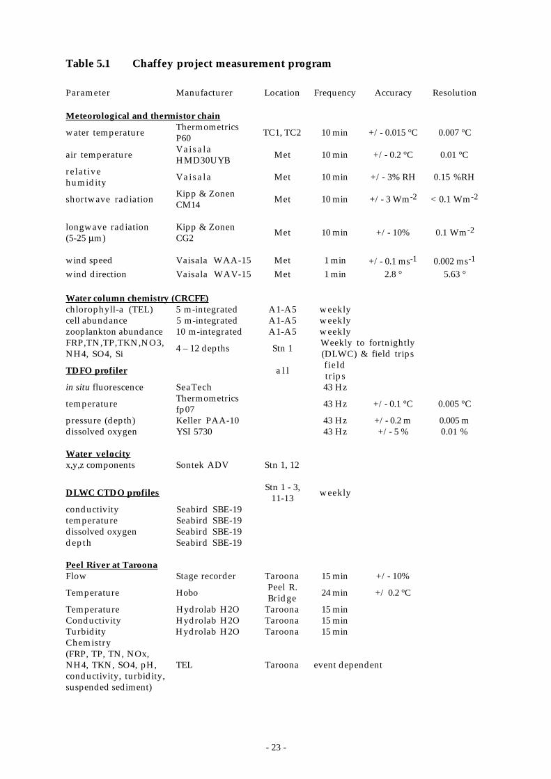
- 23 -

Table 5.1 Chaffey project measurement program

Parameter Manufacturer Location Frequency Accuracy Resolution

Meteorological and thermistor chain

water temperature ThermometricsP60 TC1, TC2 10 min +/- 0.015 °C 0.007 °C

air temperature VaisalaHMD30UYB Met 10 min +/- 0.2 °C 0.01 °C

relativehumidity Vaisala Met 10 min +/- 3% RH 0.15 %RH

shortwave radiation Kipp & ZonenCM14 Met 10 min +/- 3 Wm-2 < 0.1 Wm-2

longwave radiation(5-25 µm)

Kipp & ZonenCG2 Met 10 min +/- 10% 0.1 Wm-2

wind speed Vaisala WAA-15 Met 1 min +/- 0.1 ms-1 0.002 ms-1

wind direction Vaisala WAV-15 Met 1 min 2.8 ° 5.63 °

Water column chemistry (CRCFE)chlorophyll-a (TEL) 5 m-integrated A1-A5 weeklycell abundance 5 m-integrated A1-A5 weeklyzooplankton abundance 10 m-integrated A1-A5 weeklyFRP,TN,TP,TKN,NO3,NH4, SO4, Si 4 – 12 depths Stn 1 Weekly to fortnightly

(DLWC) & field trips

TDFO profiler a l l fieldtrips

in situ fluorescence SeaTech 43 Hz

temperature Thermometricsfp07 43 Hz +/- 0.1 °C 0.005 °C

pressure (depth) Keller PAA-10 43 Hz +/- 0.2 m 0.005 mdissolved oxygen YSI 5730 43 Hz +/- 5 % 0.01 %

Water velocity x,y,z components Sontek ADV Stn 1, 12

DLWC CTDO profiles Stn 1 - 3,

11-13 weekly

conductivity Seabird SBE-19temperature Seabird SBE-19dissolved oxygen Seabird SBE-19depth Seabird SBE-19

Peel River at Taroona Flow Stage recorder Taroona 15 min +/- 10%

Temperature Hobo Peel R.Bridge 24 min +/ 0.2 °C

Temperature Hydrolab H2O Taroona 15 minConductivity Hydrolab H2O Taroona 15 minTurbidity Hydrolab H2O Taroona 15 minChemistry(FRP, TP, TN, NOx,NH4, TKN, SO4, pH,conductivity, turbidity,suspended sediment)

TEL Taroona event dependent

- 24 -

6 Climate

6.1 Meteorology

The climate from spring through autumn at the Chaffey reservoir is characterisedby strong insolation, high temperatures and light winds (Figure 6.1). In summerthe average daily2 air temperature was 21 °C (maximum value 26 °C), the meandaily shortwave radiation 275 W m-2, and the average wind speed 2 m above thewater surface just 2.5 m s-1. The maximum shortwave radiation under clear-skyconditions was 378 W m-2, a 30% increase on the average due to the absence ofclouds. Downwelling longwave radiation averaged 360 W m-2. Afternoonthunderstorm activity was not uncommon during the summer because of therelief of the Great Dividing Range which rises 600 m above the reservoir and islocated just a few kilometres to the east.

In winter the average daily air temperature was 8 °C with a minimum value of 4°C. Mean daily shortwave and longwave radiation decreased to 105 W m-2 and305 W m-2, respectively. Winter is also calmer than summer with a mean dailywind speed of 2 m s-1. Snow often falls on the mountains.

2 The terms average daily and mean daily refer to the average value of a parameter over a 24 hourperiod commencing at midnight.

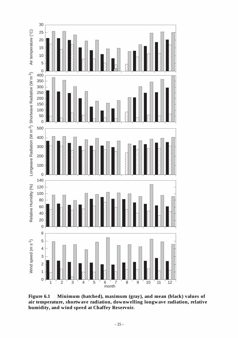
- 25 -

Win

d sp

eed

(m s

-1)

0

1

2

3

4

5

6

1 2 3 4 5 6 7 8 9 10 11 12month

0

20

40

60

80

100

120

140

Rel

ativ

e H

umid

ity (

%)

0

100

200

300

400

500

Long

wav

e R

adia

tion

(W m

-2)

050

100

150200250300

350400

Sho

rtw

ave

Rad

iatio

n (W

m-2

) 0

5

10

15

20

25

30

Air

tem

pera

ture

(°C

)

Figure 6.1 Minimum (hatched), maximum (gray), and mean (black) values ofair temperature, shortwave radiation, downwelling longwave radiation, relativehumidity, and wind speed at Chaffey Reservoir.

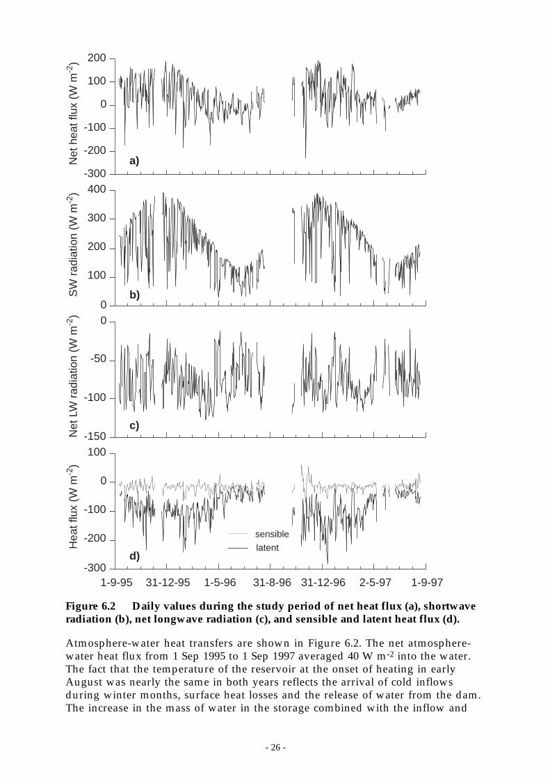
- 26 -

1-9-95 31-12-95 1-5-96 31-8-96 31-12-96 2-5-97 1-9-97

Net

hea

t flu

x (W

m-2

)S

W r

adia

tion

(W m

-2)

Net

LW

rad

iatio

n (W

m-2

)H

eat f

lux

(W m

-2)

-300

-200

-100

0

100

200

0

100

200

300

400

-150

-100

-50

0

-300

-200

-100

0

100

sensible

latent

a)

b)

c)

d)

Figure 6.2 Daily values during the study period of net heat flux (a), shortwaveradiation (b), net longwave radiation (c), and sensible and latent heat flux (d).

Atmosphere-water heat transfers are shown in Figure 6.2. The net atmosphere-water heat flux from 1 Sep 1995 to 1 Sep 1997 averaged 40 W m-2 into the water.The fact that the temperature of the reservoir at the onset of heating in earlyAugust was nearly the same in both years reflects the arrival of cold inflowsduring winter months, surface heat losses and the release of water from the dam.The increase in the mass of water in the storage combined with the inflow and

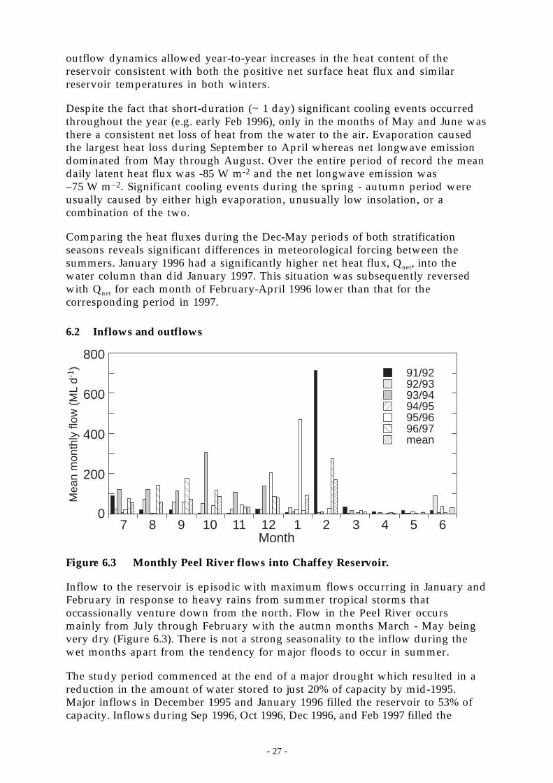
- 27 -

outflow dynamics allowed year-to-year increases in the heat content of thereservoir consistent with both the positive net surface heat flux and similarreservoir temperatures in both winters.

Despite the fact that short-duration (~ 1 day) significant cooling events occurredthroughout the year (e.g. early Feb 1996), only in the months of May and June wasthere a consistent net loss of heat from the water to the air. Evaporation causedthe largest heat loss during September to April whereas net longwave emissiondominated from May through August. Over the entire period of record the meandaily latent heat flux was -85 W m-2 and the net longwave emission was–75 W m–2. Significant cooling events during the spring - autumn period wereusually caused by either high evaporation, unusually low insolation, or acombination of the two.

Comparing the heat fluxes during the Dec-May periods of both stratificationseasons reveals significant differences in meteorological forcing between thesummers. January 1996 had a significantly higher net heat flux, Qnet, into thewater column than did January 1997. This situation was subsequently reversedwith Qnet for each month of February-April 1996 lower than that for thecorresponding period in 1997.

6.2 Inflows and outflows

0

200

400

600

800

7 8 9 10 11 12 1 2 3 4 5 6Month

91/9292/9393/9494/9595/9696/97mean

Mea

n m

onth

ly fl

ow (

ML

d-1)

Figure 6.3 Monthly Peel River flows into Chaffey Reservoir.

Inflow to the reservoir is episodic with maximum flows occurring in January andFebruary in response to heavy rains from summer tropical storms thatoccassionally venture down from the north. Flow in the Peel River occursmainly from July through February with the autmn months March - May beingvery dry (Figure 6.3). There is not a strong seasonality to the inflow during thewet months apart from the tendency for major floods to occur in summer.

The study period commenced at the end of a major drought which resulted in areduction in the amount of water stored to just 20% of capacity by mid-1995.Major inflows in December 1995 and January 1996 filled the reservoir to 53% ofcapacity. Inflows during Sep 1996, Oct 1996, Dec 1996, and Feb 1997 filled the

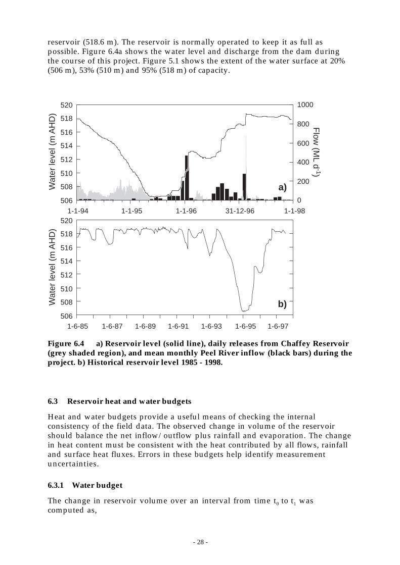
- 28 -

reservoir (518.6 m). The reservoir is normally operated to keep it as full aspossible. Figure 6.4a shows the water level and discharge from the dam duringthe course of this project. Figure 5.1 shows the extent of the water surface at 20%(506 m), 53% (510 m) and 95% (518 m) of capacity.

506

508

510

512

514

516

518

520

1-1-94 1-1-95 1-1-96 31-12-96 1-1-98

0

200

400

600

800

1000

Wat

er le

vel (

m A

HD

)

Flow

(ML d

-1)

b)506

508

510

512

514

516

518

520

Wat

er le

vel (

m A

HD

)

a)

1-6-85 1-6-87 1-6-89 1-6-91 1-6-93 1-6-95 1-6-97

Figure 6.4 a) Reservoir level (solid line), daily releases from Chaffey Reservoir(grey shaded region), and mean monthly Peel River inflow (black bars) during theproject. b) Historical reservoir level 1985 - 1998.

6.3 Reservoir heat and water budgets

Heat and water budgets provide a useful means of checking the internalconsistency of the field data. The observed change in volume of the reservoirshould balance the net inflow/outflow plus rainfall and evaporation. The changein heat content must be consistent with the heat contributed by all flows, rainfalland surface heat fluxes. Errors in these budgets help identify measurementuncertainties.

6.3.1 Water budget

The change in reservoir volume over an interval from time t0 to t1 wascomputed as,

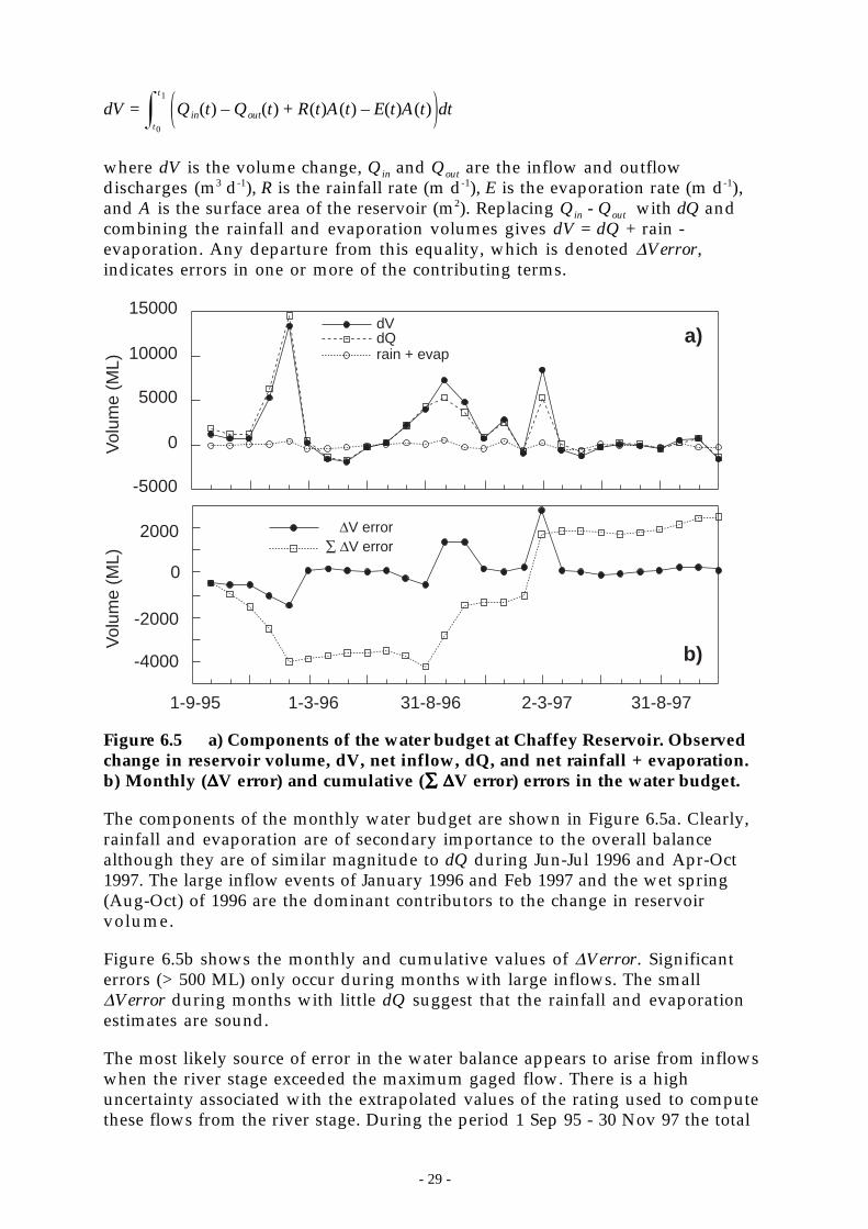
- 29 -

dV = Qin(t) – Qout(t) + R(t)A(t) – E(t)A(t) dt

t0

t1

where dV is the volume change, Qin and Qout are the inflow and outflowdischarges (m3 d-1), R is the rainfall rate (m d-1), E is the evaporation rate (m d-1),and A is the surface area of the reservoir (m2). Replacing Qin - Qout with dQ andcombining the rainfall and evaporation volumes gives dV = dQ + rain -evaporation. Any departure from this equality, which is denoted ∆Verror,indicates errors in one or more of the contributing terms.

-4000

-2000

0

2000∑ ∆V error

Vol

ume

(ML)

-5000

0

5000

10000

15000

Vol

ume

(ML)

rain + evapdQdV

1-9-95 1-3-96 31-8-96 2-3-97 31-8-97

∆V error

a)

b)

Figure 6.5 a) Components of the water budget at Chaffey Reservoir. Observedchange in reservoir volume, dV, net inflow, dQ, and net rainfall + evaporation.b) Monthly (∆∆∆∆V error) and cumulative (∑∑∑∑ ∆∆∆∆V error) errors in the water budget.

The components of the monthly water budget are shown in Figure 6.5a. Clearly,rainfall and evaporation are of secondary importance to the overall balancealthough they are of similar magnitude to dQ during Jun-Jul 1996 and Apr-Oct1997. The large inflow events of January 1996 and Feb 1997 and the wet spring(Aug-Oct) of 1996 are the dominant contributors to the change in reservoirvolume.

Figure 6.5b shows the monthly and cumulative values of ∆Verror. Significanterrors (> 500 ML) only occur during months with large inflows. The small∆Verror during months with little dQ suggest that the rainfall and evaporationestimates are sound.

The most likely source of error in the water balance appears to arise from inflowswhen the river stage exceeded the maximum gaged flow. There is a highuncertainty associated with the extrapolated values of the rating used to computethese flows from the river stage. During the period 1 Sep 95 - 30 Nov 97 the total

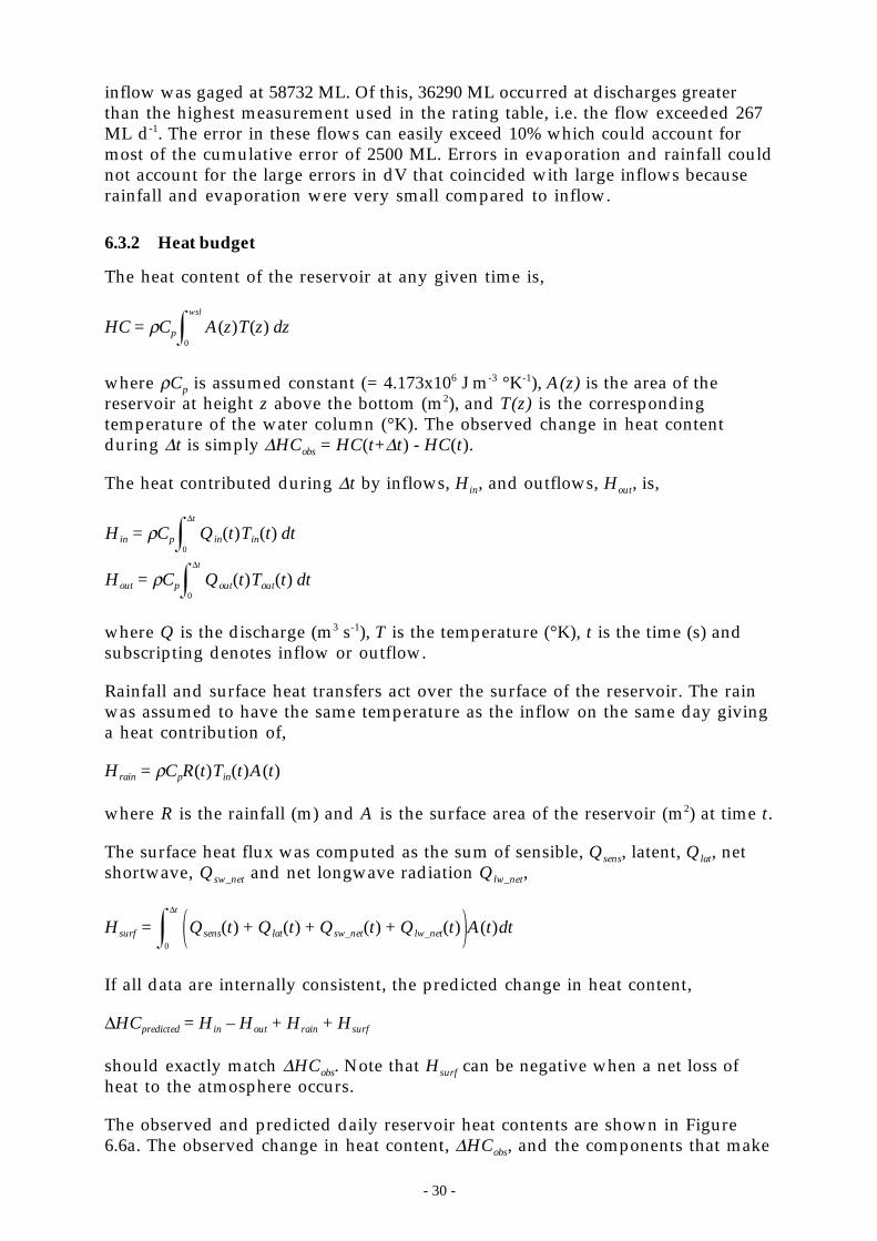
- 30 -

inflow was gaged at 58732 ML. Of this, 36290 ML occurred at discharges greaterthan the highest measurement used in the rating table, i.e. the flow exceeded 267ML d-1. The error in these flows can easily exceed 10% which could account formost of the cumulative error of 2500 ML. Errors in evaporation and rainfall couldnot account for the large errors in dV that coincided with large inflows becauserainfall and evaporation were very small compared to inflow.

6.3.2 Heat budget

The heat content of the reservoir at any given time is,

HC = ρCp A(z)T(z) dz0

wsl

where ρCp is assumed constant (= 4.173x106 J m-3 °K-1), A(z) is the area of thereservoir at height z above the bottom (m2), and T(z) is the correspondingtemperature of the water column (°K). The observed change in heat contentduring ∆t is simply ∆HCobs = HC(t+∆t) - HC(t).

The heat contributed during ∆t by inflows, Hin, and outflows, Hout, is,

Hin = ρCp Qin(t)Tin(t) dt0

∆t

Hout = ρCp Qout(t)Tout(t) dt0

∆t

where Q is the discharge (m3 s-1), T is the temperature (°K), t is the time (s) andsubscripting denotes inflow or outflow.

Rainfall and surface heat transfers act over the surface of the reservoir. The rainwas assumed to have the same temperature as the inflow on the same day givinga heat contribution of,

Hrain = ρCpR(t)Tin(t)A(t)

where R is the rainfall (m) and A is the surface area of the reservoir (m2) at time t.

The surface heat flux was computed as the sum of sensible, Qsens, latent, Qlat, netshortwave, Qsw_net and net longwave radiation Qlw_net,

Hsurf = Qsens(t) + Qlat(t) + Qsw_net(t) + Qlw_net(t) A(t)dt

0

∆t

If all data are internally consistent, the predicted change in heat content,

∆HCpredicted = Hin – Hout + Hrain + Hsurf

should exactly match ∆HCobs. Note that Hsurf can be negative when a net loss ofheat to the atmosphere occurs.

The observed and predicted daily reservoir heat contents are shown in Figure6.6a. The observed change in heat content, ∆HCobs, and the components that make

- 31 -

up ∆HCpredicted are shown, computed on a monthly basis, in Figure 6.6b wheresurface heat transfers and rainfall have been combined because they both actupon the same surface area. There is clearly a large discrepancy between observedand predicted heat contents.

The potentially major sources of error are: inflow volumes; reservoir volume;and surface heat fluxes including rain. The quantities ∆HCerror, ∆HQerror, and∆HCresidual shown in Figure 6.6c represent respectively the difference betweenobserved and predicted changes in heat contents, the heat contribution associatedwith the error in the water balance, and the residual error in the heat budget afteradjusting for the water balance error. After correcting ∆HCpredicted for the heatcontained in the water balance error, the residual error in the heat budget isconsistently negative and varies between 1 and 3% of the total reservoir heatcontent with a mean value of 2%.

The most likely explanation for the residual heat budget error is that the storagetable (area vs depth) for the reservoir is biased and underestimates areas by 2%from their actual values. The corresponding heat content would then beunderestimated by a similar percentage. This is not an unreasonable error giventhat storage tables are derived from contour maps using planimetry. An error inmeasuring the mean reservoir temperature of nearly -4.5°C, which is notpossible, would be required to produce a comparable heat content error.

6.3.3 ConclusionHeat and water budget calculations have highlighted the errors associated withstreamflow and reservoir volume measurements. Water balance calculationsshowed that 62% of the total inflow to the reservoir occurred at river stagesexceeding the highest measured flow. Uncertainty in the rating of the Taroonastreamflow gage at high flows is the most likely explanation for the observedimbalance in the water budget.

The total heat contributed by inflow during the project was comparable to theheat content of the reservoir when full and approximately 6 times greater thanthe total heat supplied from surface heat fluxes. Heat budget calculations, aftercorrection for the heat content of the water budget volume error, consistentlyunderestimated reservoir heat content by 2%. This suggests that the storage tableis biased and that areas should be increased by a corresponding amount. Otherpossible sources of error associated with calculated surface heat fluxes, rainfall,horizontal variability in temperature make only a minor contribution to theerror in the heat budget calculations.

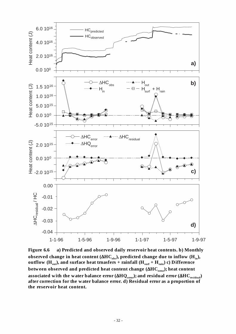
- 32 -

-2.0 1015

0.0 100

2.0 1015

∆HCerror

∆HQerror

∆HCresidual

-5.0 1015

0.0 100

5.0 1015

1.0 1016

1.5 1016∆HC

obsH

in

Hout

Hsurf

+ Hrain

-0.04

-0.02

0.00

1-1-96 1-5-96 1-9-96 1-1-97 1-5-97 1-9-97

Hea

t con

tent

(J)

Hea

t con

tent

(J)

∆HC

resi

dual

/ H

C -0.01

-0.03

0.0 100

2.0 1016

4.0 1016

6.0 1016HCpredicted

HCobserved

Hea

t con

tent

(J)

a)

b)

c)

d)

Figure 6.6 a) Predicted and observed daily reservoir heat contents. b) Monthlyobserved change in heat content (∆∆∆∆HCobs), predicted change due to inflow (Hin),outflow (Hout), and surface heat trnasfers + rainfall (Hsurf + Hrain) c) Differencebetween observed and predicted heat content change (∆∆∆∆HCerror); heat contentassociated with the water balance error (∆∆∆∆HQerror); and residual error (∆∆∆∆HCresidual)after correction for the water balance error. d) Residual error as a proportion ofthe reservoir heat content.

- 33 -

7 Transport processes

The physical transport processes in the reservoir establish the conditions underwhich the phytoplankton must grow. Of particular concern are changes in thedepth of the surface layer, which governs the light climate, and the supply ofnutrients to the water column, and especially to the euphotic zone. Atmosphericconditions and thermal stratification in the water column are the mostsignificant factors controlling the depth of the surface mixed layer. Inflow eventsintroduce sediments and nutrients from the catchment and transport themhorizontally into the water column. Turbulent diffusion, surface layer deepening,and large-scale circulation caused by artificial destratification and differentialcooling transport nutrients upwards from the sediments to the euphotic zone.Boundary mixing caused by both surface and internal waves breaking along theshoreline can liberate nutrients from the sediments and transport them laterally.

In this chapter we examine the most important transport processes in thereservoir. This information will then provide the physical context of the biologyand chemistry in the chapters that follow.

7.1 Inflow events

When the sediment-laden inflows typical of the Peel River enter the reservoirthey first mix with the ambient water at the upstream (south) end of the dam andthen they plunge to a level where the density of the inflowing water matches thatof the undisturbed water column. This is called the ‘level of neutral buoyancy’and depends mainly on the temperatures of the inflow and the water at theupstream end of the storage. Our measurements showed significant changes inthe temperature of the inflow over the 6.7 km between Taroona, wheretemperature has been measured historically, and immediately upstream of thereservoir; this has significant implications for accurately predicting the level atwhich the intrusion will form.

The inflow intrudes into the rest of the basin at the level of neutral buoyancycarrying with it nutrients and suspended sediment. As the intrusion proceedstowards the dam wall it spreads out laterally and decelerates. This allows thelarger sediment particles to sink out of the intrusion. The shallowness and gentleslope at the south end of the reservoir (Figure 5.1) ensure that significant mixingof the inflowing water with reservoir water can occur for up to 2 km (dependingon reservoir level) after the river enters the reservoir, after which inflows mayplunge and intrude into the deeper main basin.

The two largest inflow events during the study occurred in January 1996 andFebruary 1997 (Figure 6.3). In both cases the inflow intrusion propagated into thewater column below the surface mixed layer. The January 1996 inflow was veryturbid and intruded below a depth of 11 m while the destratifier was operating.Approximately 2 days after the flood peak was recorded at the Taroona gaugingstation, water within the bubble plumes became muddy while the surroundingwater remained relatively clear, implying that the intrusion had finally arrived atthe dam wall.

- 34 -

The 13-16 February 1997 inflow produced an intrusion with high nutrientconcentrations and a very strong conductivity signature (Figure 7.1). Theconductivity profile on 11-02 shows the conditions in the dam prior to the inflow.One week after the inflow, the conductivity profile on 21-02 shows a prominentintrusion of lower conductivity water between 4 and 11 m depth. The intrusioncontained very high phosphorus concentrations and increased the TPconcentration at a depth of 10 m by over 100 µg L-1 from pre-inflow value (Figure7.1, bottom); most of the increase in TP was in the form of FRP. The intrusionremained relatively undisturbed between 4-12 m through 4 Mar 97. During thefollowing weeks autumnal cooling caused the surface layer to deepen (heavy line,Figure 7.1, top) which lowered the top of the intrusion’s conductivity signature aswater from the top of the intrusion was entrained into the surface layer. Surfacelayer FRP and TP concentrations increased as a result of the entrainment and aspurt of algal growth followed immediately (Section 9.2.4.1). The magnitude ofthe conductivity peak diminished as well due to a combination of diffusivetransport and, presumably, in-situ chemical reactions affecting CO2

concentrations. This illustrates vividly how vital both the surface layer dynamicsand the inflow temperature are in determining the response of the reservoir toexternal contaminant loads.

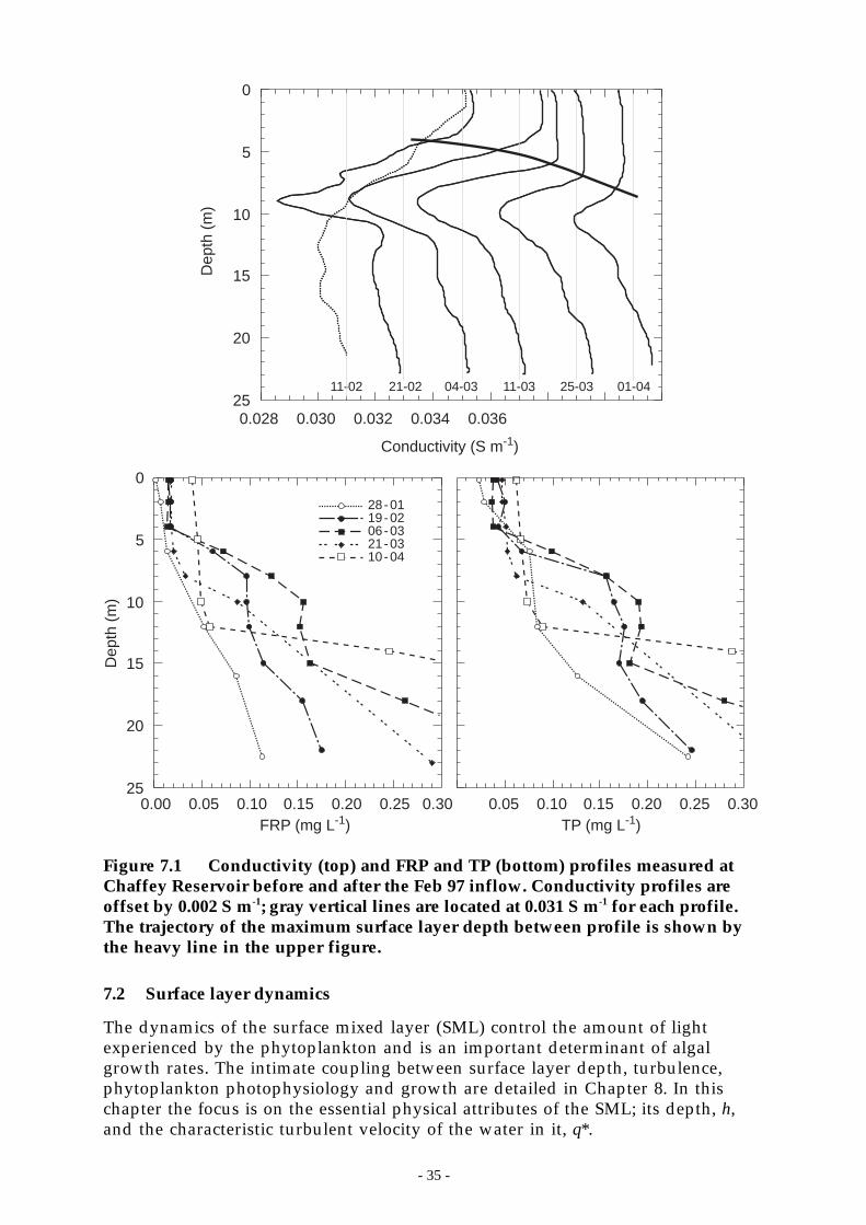
- 35 -

0

5

10

15

20

250.028 0.030 0.032 0.034 0.036

11-02 21-02 04-03 11-03 25-03 01-04

Dep

th (

m)

Conductivity (S m-1)

0

5

10

15

20

25

FRP (mg L-1)

Dep

th (

m)

TP (mg L-1)

06-0321-0310-04

19-0228-01

0.00 0.05 0.10 0.15 0.20 0.25 0.30 0.05 0.10 0.15 0.20 0.25 0.30

Figure 7.1 Conductivity (top) and FRP and TP (bottom) profiles measured atChaffey Reservoir before and after the Feb 97 inflow. Conductivity profiles areoffset by 0.002 S m-1; gray vertical lines are located at 0.031 S m-1 for each profile.The trajectory of the maximum surface layer depth between profile is shown bythe heavy line in the upper figure.

7.2 Surface layer dynamics

The dynamics of the surface mixed layer (SML) control the amount of lightexperienced by the phytoplankton and is an important determinant of algalgrowth rates. The intimate coupling between surface layer depth, turbulence,phytoplankton photophysiology and growth are detailed in Chapter 8. In thischapter the focus is on the essential physical attributes of the SML; its depth, h,and the characteristic turbulent velocity of the water in it, q*.

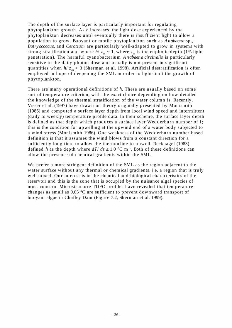
- 36 -

The depth of the surface layer is particularly important for regulatingphytoplankton growth. As h increases, the light dose experienced by thephytoplankton decreases until eventually there is insufficient light to allow apopulation to grow. Buoyant or motile phytoplankton such as Anabaena sp.,Botryococcus, and Ceratium are particularly well-adapted to grow in systems withstrong stratification and where h/zeu ~ 1, where zeu is the euphotic depth (1% lightpenetration). The harmful cyanobacterium Anabaena circinalis is particularlysensitive to the daily photon dose and usually is not present in significantquantities when h/zeu > 3 (Sherman et al. 1998). Artificial destratification is oftenemployed in hope of deepening the SML in order to light-limit the growth ofphytoplankton.

There are many operational definitions of h. These are usually based on somesort of temperature criterion, with the exact choice depending on how detailedthe knowledge of the thermal stratification of the water column is. Recently,Visser et al. (1997) have drawn on theory originally presented by Monismith(1986) and computed a surface layer depth from local wind speed and intermittent(daily to weekly) temperature profile data. In their scheme, the surface layer depthis defined as that depth which produces a surface layer Wedderburn number of 1;this is the condition for upwelling at the upwind end of a water body subjected toa wind stress (Monismith 1986). One weakness of the Wedderburn number-baseddefinition is that it assumes the wind blows from a constant direction for asufficiently long time to allow the thermocline to upwell. Recknagel (1983)defined h as the depth where dT/dz ≥ 1.0 °C m-1. Both of these definitions canallow the presence of chemical gradients within the SML.

We prefer a more stringent definition of the SML as the region adjacent to thewater surface without any thermal or chemical gradients, i.e. a region that is trulywell-mixed. Our interest is in the chemical and biological characteristics of thereservoir and this is the zone that is occupied by the nuisance algal species ofmost concern. Microstructure TDFO profiles have revealed that temperaturechanges as small as 0.05 °C are sufficient to prevent downward transport ofbuoyant algae in Chaffey Dam (Figure 7.2, Sherman et al. 1999).

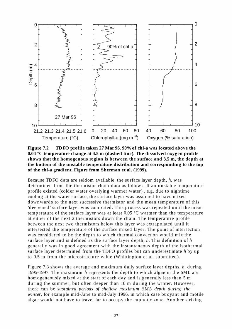
- 37 -

21.2 21.3 21.4 21.5 21.6

0

2

4

6

8

10

Temperature (°C)

Dep

th (

m)

27 Mar 96

40 60 80 100

0

2

4

6

8

10

Oxygen (% saturation)

0 20 40 60 80

Chlorophyll-a (mg m -3)

90% of chl-a

Figure 7.2 TDFO profile taken 27 Mar 96. 90% of chl-a was located above the0.04 °C temperature change at 4.5 m (dashed line). The dissolved oxygen profileshows that the homogenous region is between the surface and 3.5 m, the depth atthe bottom of the unstable temperature distribution and corresponding to the topof the chl-a gradient. Figure from Sherman et al. (1999).

Because TDFO data are seldom available, the surface layer depth, h, wasdetermined from the thermistor chain data as follows. If an unstable temperatureprofile existed (colder water overlying warmer water) , e.g. due to nightimecooling at the water surface, the surface layer was assumed to have mixeddownwards to the next successive thermistor and the mean temperature of this‘deepened’ surface layer was computed. This process was repeated until the meantemperature of the surface layer was at least 0.05 °C warmer than the temperatureat either of the next 2 thermistors down the chain. The temperature profilebetween the next two thermistors below this layer was extrapolated until itintersected the temperature of the surface mixed layer. The point of intersectionwas considered to be the depth to which thermal convection would mix thesurface layer and is defined as the surface layer depth, h. This definition of hgenerally was in good agreement with the instantaneous depth of the isothermalsurface layer determined from the TDFO profiles but can underestimate h by upto 0.5 m from the microstructure value (Whittington et al. submitted).

Figure 7.3 shows the average and maximum daily surface layer depths, h, during1995-1997. The maximum h represents the depth to which algae in the SML arehomogeneously mixed at the start of each day and is generally less than 5 mduring the summer, but often deeper than 10 m during the winter. However,there can be sustained periods of shallow maximum SML depth during thewinter, for example mid-June to mid-July 1996, in which case buoyant and motilealgae would not have to travel far to occupy the euphotic zone. Another striking

- 38 -

feature is that the average daily h is usually significantly less than 5 m at all timesof year. Notice also that the SML was deeper during winter 1997 than in winter1996. The difference may be due in part to the deeper water column in 1997,which reduced the horizontal temperature gradients produced by differentialcooling (section 7.5) and thereby reduced the vertical temperature gradients aswell (i.e. decreased temperature differential across a deeper water column).

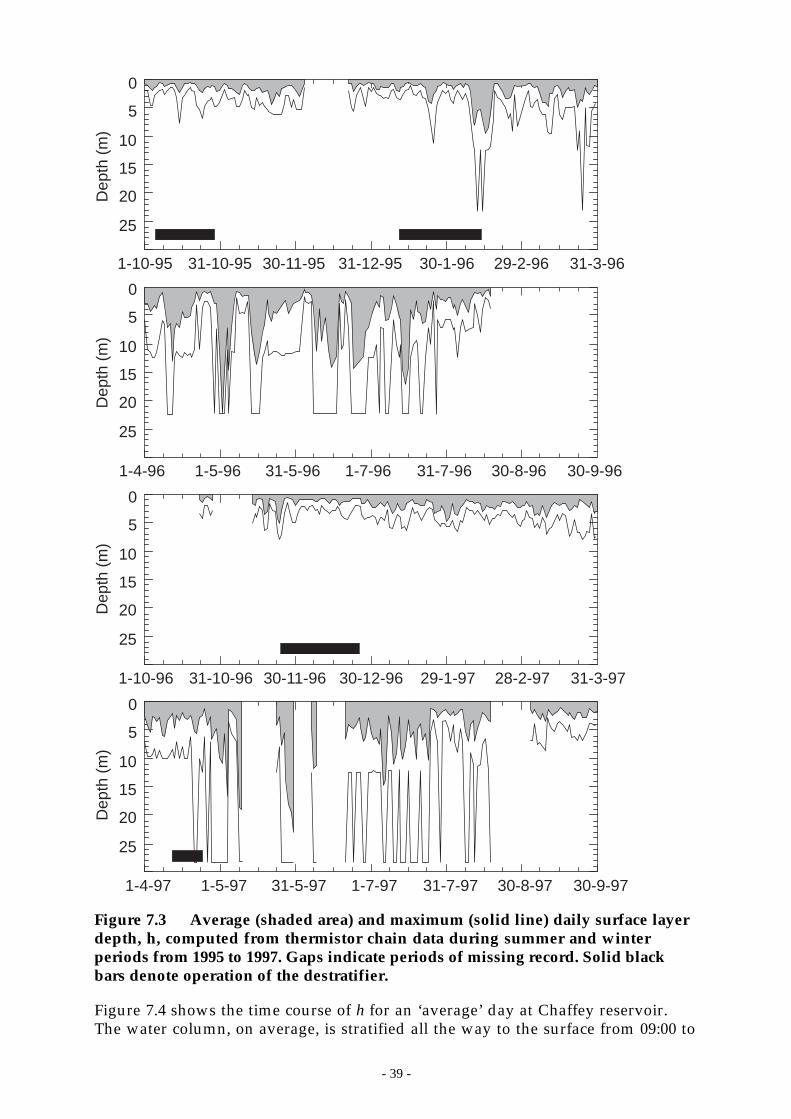
- 39 -

1-10-95 31-10-95 30-11-95 31-12-95 30-1-96 29-2-96 31-3-96

1-10-96 31-10-96 30-11-96 30-12-96 29-1-97 28-2-97 31-3-97

1-4-96 1-5-96 31-5-96 1-7-96 31-7-96 30-8-96 30-9-96

1-4-97 1-5-97 31-5-97 1-7-97 31-7-97 30-8-97 30-9-97

0

5

10

15

20

25

0

5

10

15

20

25

0

5

10

15

20

25

0

5

10

15

20

25

Dep

th (

m)

Dep

th (

m)

Dep

th (

m)

Dep

th (

m)

Figure 7.3 Average (shaded area) and maximum (solid line) daily surface layerdepth, h, computed from thermistor chain data during summer and winterperiods from 1995 to 1997. Gaps indicate periods of missing record. Solid blackbars denote operation of the destratifier.

Figure 7.4 shows the time course of h for an ‘average’ day at Chaffey reservoir.The water column, on average, is stratified all the way to the surface from 09:00 to

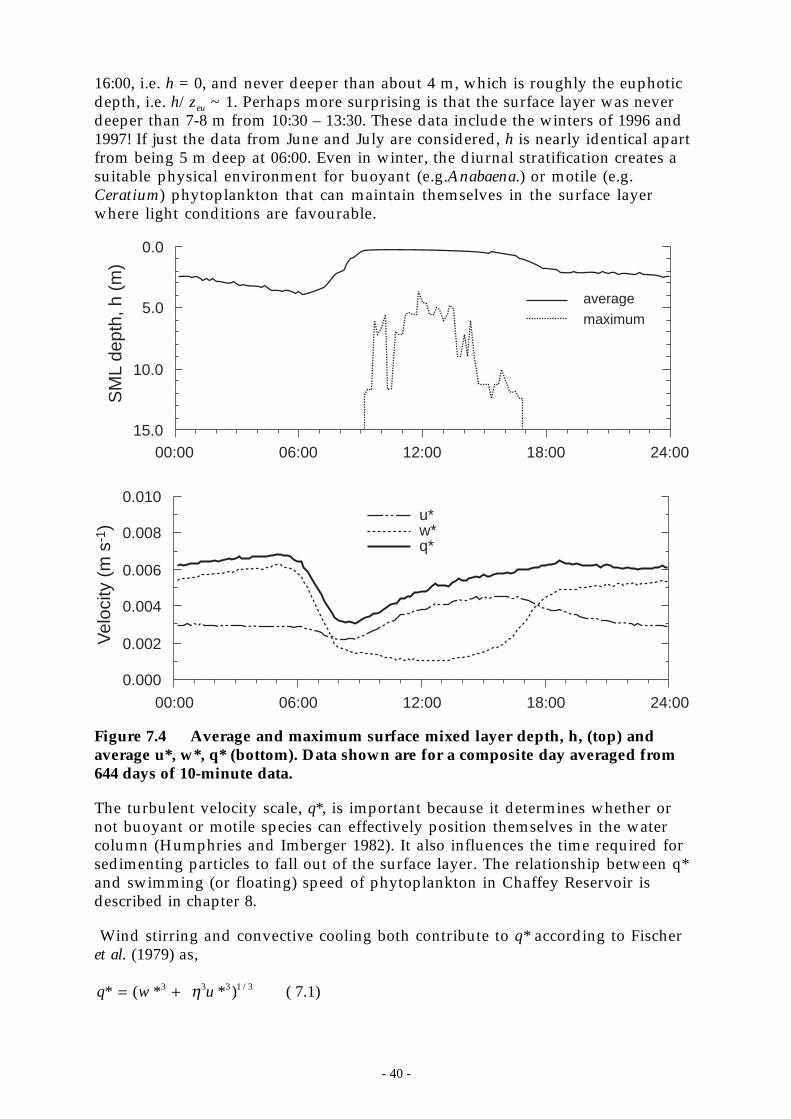
- 40 -

16:00, i.e. h = 0, and never deeper than about 4 m, which is roughly the euphoticdepth, i.e. h/zeu ~ 1. Perhaps more surprising is that the surface layer was neverdeeper than 7-8 m from 10:30 – 13:30. These data include the winters of 1996 and1997! If just the data from June and July are considered, h is nearly identical apartfrom being 5 m deep at 06:00. Even in winter, the diurnal stratification creates asuitable physical environment for buoyant (e.g.Anabaena.) or motile (e.g.Ceratium) phytoplankton that can maintain themselves in the surface layerwhere light conditions are favourable.

0.000

0.002

0.004

0.006

0.008

0.010u*w*q*

00:00 06:00 12:00 18:00 24:00

Vel

ocity

(m

s-1

)S

ML

dept

h, h

(m

)

average

maximum

0.0

5.0

10.0

15.000:00 06:00 12:00 18:00 24:00

Figure 7.4 Average and maximum surface mixed layer depth, h, (top) andaverage u*, w*, q* (bottom). Data shown are for a composite day averaged from644 days of 10-minute data.

The turbulent velocity scale, q*, is important because it determines whether ornot buoyant or motile species can effectively position themselves in the watercolumn (Humphries and Imberger 1982). It also influences the time required forsedimenting particles to fall out of the surface layer. The relationship between q*and swimming (or floating) speed of phytoplankton in Chaffey Reservoir isdescribed in chapter 8.

Wind stirring and convective cooling both contribute to q* according to Fischeret al. (1979) as,

q w u* ( * * ) /= +3 3 3 1 3η ( 7.1)

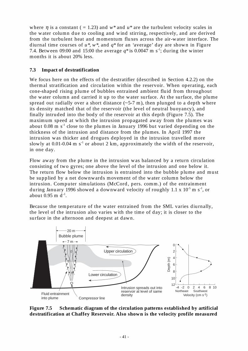
- 41 -

where η is a constant ( = 1.23) and w* and u* are the turbulent velocity scales inthe water column due to cooling and wind stirring, respectively, and are derivedfrom the turbulent heat and momentum fluxes across the air-water interface. Thediurnal time courses of u*, w*, and q* for an ‘average’ day are shown in Figure7.4. Between 09:00 and 15:00 the average q* is 0.0047 m s-1; during the wintermonths it is about 20% less.

7.3 Impact of destratification

We focus here on the effects of the destratifier (described in Section 4.2.2) on thethermal stratification and circulation within the reservoir. When operating, eachcone-shaped rising plume of bubbles entrained ambient fluid from throughoutthe water column and carried it up to the water surface. At the surface, the plumespread out radially over a short distance (~5-7 m), then plunged to a depth whereits density matched that of the reservoir (the level of neutral buoyancy), andfinally intruded into the body of the reservoir at this depth (Figure 7.5). Themaximum speed at which the intrusion propagated away from the plumes wasabout 0.08 m s-1 close to the plumes in January 1996 but varied depending on thethickness of the intrusion and distance from the plumes. In April 1997 theintrusion was thicker and drogues deployed in the intrusion travelled moreslowly at 0.01-0.04 m s-1 or about 2 km, approximately the width of the reservoir,in one day.

Flow away from the plume in the intrusion was balanced by a return circulationconsisting of two gyres; one above the level of the intrusion and one below it.The return flow below the intrusion is entrained into the bubble plume and mustbe supplied by a net downwards movement of the water column below theintrusion. Computer simulations (McCord, pers. comm.) of the entrainmentduring January 1996 showed a downward velocity of roughly 1.1 x 10-5 m s-1, orabout 0.95 m d-1.

Because the temperature of the water entrained from the SML varies diurnally,the level of the intrusion also varies with the time of day; it is closer to thesurface in the afternoon and deepest at dawn.

Fluid entrainmentinto plume Compressor line

Lower circulation

Bubble plume

Intrusion spreads out intoreservoir at level of samedensity

Upper circulation

7 m

20 m

Velocity (cm s-1)Northeast Southwest-4 -2 0 2 4 6 8 10

Dep

th (

m)

0

2

4

6

8

10

12

Figure 7.5 Schematic diagram of the circulation patterns established by artificialdestratification at Chaffey Reservoir. Also shown is the velocity profile measured

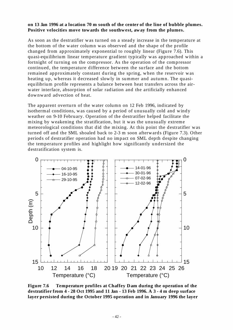
- 42 -

on 13 Jan 1996 at a location 70 m south of the center of the line of bubble plumes.Positive velocities move towards the southwest, away from the plumes.

As soon as the destratifier was turned on a steady increase in the temperature atthe bottom of the water column was observed and the shape of the profilechanged from approximately exponential to roughly linear (Figure 7.6). Thisquasi-equilibrium linear temperature gradient typically was approached within afortnight of turning on the compressor. As the operation of the compressorcontinued, the temperature difference between the surface and the bottomremained approximately constant during the spring, when the reservoir washeating up, whereas it decreased slowly in summer and autumn. The quasi-equilibrium profile represents a balance between heat transfers across the air-water interface, absorption of solar radiation and the artificially enhanceddownward advection of heat.

The apparent overturn of the water column on 12 Feb 1996, indicated byisothermal conditions, was caused by a period of unusually cold and windyweather on 9-10 February. Operation of the destratifier helped facilitate themixing by weakening the stratification, but it was the unusually extrememeteorological conditions that did the mixing. At this point the destratifier wasturned off and the SML shoaled back to 2-3 m soon afterwards (Figure 7.3). Otherperiods of destratifier operation had no impact on SML depth despite changingthe temperature profiles and highlight how significantly undersized thedestratification system is.

19 20 21 22 23 24 25 26

14-01-9630-01-9607-02-9612-02-96

0

5

10

15

Temperature (°C)10 12 14 16 18 20

0

5

10

15

04-10-9516-10-9529-10-95

Temperature (°C)

Dep

th (

m)

Figure 7.6 Temperature profiles at Chaffey Dam during the operation of thedestratifier from 4 - 28 Oct 1995 and 11 Jan - 13 Feb 1996. A 3 - 4 m deep surfacelayer persisted during the October 1995 operation and in January 1996 the layer

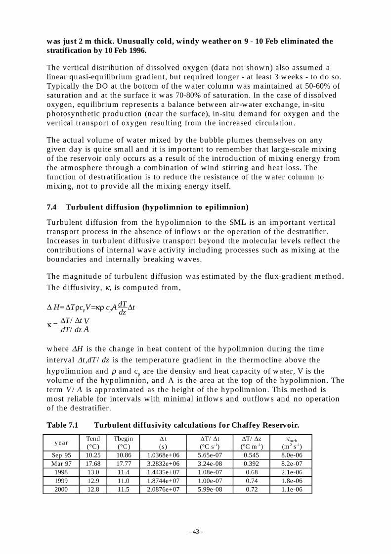
- 43 -

was just 2 m thick. Unusually cold, windy weather on 9 - 10 Feb eliminated thestratification by 10 Feb 1996.

The vertical distribution of dissolved oxygen (data not shown) also assumed alinear quasi-equilibrium gradient, but required longer - at least 3 weeks - to do so.Typically the DO at the bottom of the water column was maintained at 50-60% ofsaturation and at the surface it was 70-80% of saturation. In the case of dissolvedoxygen, equilibrium represents a balance between air-water exchange, in-situphotosynthetic production (near the surface), in-situ demand for oxygen and thevertical transport of oxygen resulting from the increased circulation.

The actual volume of water mixed by the bubble plumes themselves on anygiven day is quite small and it is important to remember that large-scale mixingof the reservoir only occurs as a result of the introduction of mixing energy fromthe atmosphere through a combination of wind stirring and heat loss. Thefunction of destratification is to reduce the resistance of the water column tomixing, not to provide all the mixing energy itself.

7.4 Turbulent diffusion (hypolimnion to epilimnion)

Turbulent diffusion from the hypolimnion to the SML is an important verticaltransport process in the absence of inflows or the operation of the destratifier.Increases in turbulent diffusive transport beyond the molecular levels reflect thecontributions of internal wave activity including processes such as mixing at theboundaries and internally breaking waves.

The magnitude of turbulent diffusion was estimated by the flux-gradient method.The diffusivity, κ, is computed from,

∆ H=∆TρcpV=κρ cpAdTdz

∆t

κ = ∆T/∆tdT/dz

VA

where ∆H is the change in heat content of the hypolimnion during the timeinterval ∆t,dT/dz is the temperature gradient in the thermocline above thehypolimnion and ρ and cp are the density and heat capacity of water, V is thevolume of the hypolimnion, and A is the area at the top of the hypolimnion. Theterm V/A is approximated as the height of the hypolimnion. This method ismost reliable for intervals with minimal inflows and outflows and no operationof the destratifier.

Table 7.1 Turbulent diffusivity calculations for Chaffey Reservoir.

year Tend(°C)

Tbegin(°C)

∆ t(s)

∆T/∆t(°C s-1)

∆T/∆z(°C m-1)

κturb

(m2 s-1)Sep 95 10.25 10.86 1.0368e+06 5.65e-07 0.545 8.0e-06Mar 97 17.68 17.77 3.2832e+06 3.24e-08 0.392 8.2e-071998 13.0 11.4 1.4435e+07 1.08e-07 0.68 2.1e-061999 12.9 11.0 1.8744e+07 1.00e-07 0.74 1.8e-062000 12.8 11.5 2.0876e+07 5.99e-08 0.72 1.1e-06

- 44 -

Two periods were chosen for the calculation: 11-23 Sep 1995 and 6 Mar-13 Apr1997. These periods had little or no inflow and a positive net heat flux into thewater column. During spring 1995, the calculated κ was 80 times greater than themolecular value whereas in autumn 1997 it was 8 time greater. The results areshown in Table 7.1 which also gives seasonal estimates of turbulent diffusivitycomputed from fortnightly CTDO profiler data collected by DLWC during 1997-2000. The lower values are more typical of conditions in the reservoir duringsummer and autumn. In comparison, the downward advective transport of heatcaused by operation of the destratifier would be equivalent to a turbulentdiffusivity 1000 times greater than the molecular rate.

The flux-gradient method is commonly used to estimate turbulent diffusivity inlakes and oceans and provides a basin-wide average of vertical transport(Imberger 1998; Wüest and Gloor 1998). A reasonably universal finding is thatthis average transport is typically 10-100 times faster than molecular rates. Most ofthe time Chaffey Reservoir falls at the low end of this range, presumably a resultof the mild climate and light winds. Another common finding is that transportoccurs at near molecular rates in pelagic regions implying that the overwhelmingmajority of transport and mixing occurring in the benthic boundary layer. Thislatter result is consistent with the higher turbulent diffusivity computed forChaffey reservoir in Sep 1995 when the storage was just 20% full and would havehad a much higher ratio of benthic boundary layer volume to total reservoirvolume as compared to Mar 1997.

7.5 Differential cooling

When heat is lost from the water surface, the SML temperature decreases at auniform rate across the reservoir surface until the SML deepens to the sediment.This occurs first at the edge of the reservoir where the water is shallow. Since allof the heat loss comes from the SML, once it deepens to the bottom in theshallower regions, these areas become colder more quickly than the rest of thereservoir where the SML is still deepening. As the cooling continues, ahorizontal temperature gradient is established where water in the shallow areasis colder than water at the same depth in the deeper areas. The horizontaltemperature gradient produces a density current in which denser (colder) waterfrom the shallows flows along the bottom of the reservoir until it reaches itslevel of neutral buoyancy at which point it intrudes into the main basin of thereservoir. Figure 7.7 shows the circulation for the case where the intrusion occursalong the bottom. This process is called differential cooling. Given its ubiquitousnature it is surprising that relatively few field studies have examined it in detail(e.g., Wells and Sherman, accepted; Sturman et al., 1999; Finnigan and Ivey, 1999;Monismith et al., 1990).

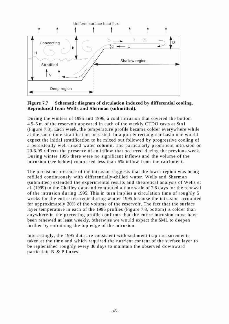
- 45 -

D

hH

Deep region

Shallow region

Convecting

Stratified

U

V

Uniform surface heat flux

d

Figure 7.7 Schematic diagram of circulation induced by differential cooling.Reproduced from Wells and Sherman (submitted).

During the winters of 1995 and 1996, a cold intrusion that covered the bottom4.5–5 m of the reservoir appeared in each of the weekly CTDO casts at Stn1(Figure 7.8). Each week, the temperature profile became colder everywhere whileat the same time stratification persisted. In a purely rectangular basin one wouldexpect the initial stratification to be mixed out followed by progressive cooling ofa persistently well-mixed water column. The particularly prominent intrusion on20-6-95 reflects the presence of an inflow that occurred during the previous week.During winter 1996 there were no significant inflows and the volume of theintrusion (see below) comprised less than 5% inflow from the catchment.

The persistent presence of the intrusion suggests that the lower region was beingrefilled continuously with differentially-chilled water. Wells and Sherman(submitted) extended the experimental results and theoretical analysis of Wells etal. (1999) to the Chaffey data and computed a time scale of 7.6 days for the renewalof the intrusion during 1995. This in turn implies a circulation time of roughly 5weeks for the entire reservoir during winter 1995 because the intrusion accountedfor approximately 20% of the volume of the reservoir. The fact that the surfacelayer temperature in each of the 1996 profiles (Figure 7.8, bottom) is colder thananywhere in the preceding profile confirms that the entire intrusion must havebeen renewed at least weekly, otherwise we would expect the SML to deepenfurther by entraining the top edge of the intrusion.

Interestingly, the 1995 data are consistent with sediment trap measurementstaken at the time and which required the nutrient content of the surface layer tobe replenished roughly every 30 days to maintain the observed downwardparticulate N & P fluxes.

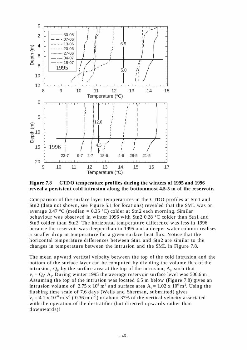
- 46 -

9 10 11 12 13 14 15 16 17

0

5

10

15

2021-528-54-618-62-79-723-7

Temperature (°C)

1996

Dep

th (

m) 12.0

4.5

0

2

4

6

8

10

12

Dep

th (

m)

8 9 10 11 12 13 14 15

30-0507-0613-0620-0627-0604-0718-07

Temperature (°C)

6.5

5.01995

Figure 7.8 CTDO temperature profiles during the winters of 1995 and 1996reveal a persistent cold intrusion along the bottommost 4.5-5 m of the reservoir.

Comparison of the surface layer temperatures in the CTDO profiles at Stn1 andStn2 (data not shown, see Figure 5.1 for locations) revealed that the SML was onaverage 0.47 °C (median = 0.35 °C) colder at Stn2 each morning. Similarbehaviour was observed in winter 1996 with Stn2 0.28 °C colder than Stn1 andStn3 colder than Stn2. The horizontal temperature difference was less in 1996because the reservoir was deeper than in 1995 and a deeper water column realisesa smaller drop in temperature for a given surface heat flux. Notice that thehorizontal temperature differences between Stn1 and Stn2 are similar to thechanges in temperature between the intrusion and the SML in Figure 7.8.

The mean upward vertical velocity between the top of the cold intrusion and thebottom of the surface layer can be computed by dividing the volume flux of theintrusion, Qi, by the surface area at the top of the intrusion, Ai, such thatvi = Qi/Ai. During winter 1995 the average reservoir surface level was 506.6 m.Assuming the top of the intrusion was located 6.5 m below (Figure 7.8) gives anintrusion volume of 2.75 x 106 m3 and surface area Ai = 1.02 x 106 m2. Using theflushing time scale of 7.6 days (Wells and Sherman, submitted) givesvi = 4.1 x 10–6 m s-1 ( 0.36 m d-1) or about 37% of the vertical velocity associatedwith the operation of the destratifier (but directed upwards rather thandownwards)!

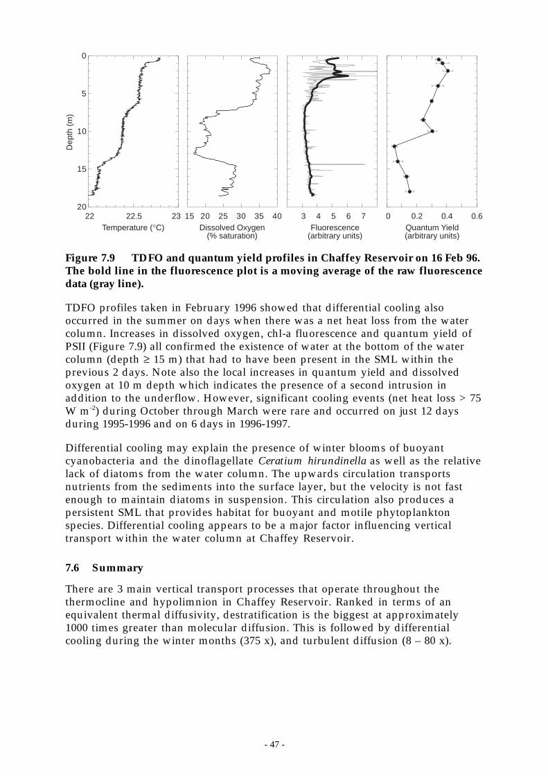
- 47 -

0

5

10

15

203 4 5 6 7

Fluorescence(arbitrary units)

15 20 25 30 35 40Dissolved Oxygen

(% saturation)

22 22.5 23Temperature (°C)

0 0.2 0.4 0.6Quantum Yield(arbitrary units)

Dep

th (

m)

Figure 7.9 TDFO and quantum yield profiles in Chaffey Reservoir on 16 Feb 96.The bold line in the fluorescence plot is a moving average of the raw fluorescencedata (gray line).

TDFO profiles taken in February 1996 showed that differential cooling alsooccurred in the summer on days when there was a net heat loss from the watercolumn. Increases in dissolved oxygen, chl-a fluorescence and quantum yield ofPSII (Figure 7.9) all confirmed the existence of water at the bottom of the watercolumn (depth ≥ 15 m) that had to have been present in the SML within theprevious 2 days. Note also the local increases in quantum yield and dissolvedoxygen at 10 m depth which indicates the presence of a second intrusion inaddition to the underflow. However, significant cooling events (net heat loss > 75W m-2) during October through March were rare and occurred on just 12 daysduring 1995-1996 and on 6 days in 1996-1997.

Differential cooling may explain the presence of winter blooms of buoyantcyanobacteria and the dinoflagellate Ceratium hirundinella as well as the relativelack of diatoms from the water column. The upwards circulation transportsnutrients from the sediments into the surface layer, but the velocity is not fastenough to maintain diatoms in suspension. This circulation also produces apersistent SML that provides habitat for buoyant and motile phytoplanktonspecies. Differential cooling appears to be a major factor influencing verticaltransport within the water column at Chaffey Reservoir.

7.6 Summary

There are 3 main vertical transport processes that operate throughout thethermocline and hypolimnion in Chaffey Reservoir. Ranked in terms of anequivalent thermal diffusivity, destratification is the biggest at approximately1000 times greater than molecular diffusion. This is followed by differentialcooling during the winter months (375 x), and turbulent diffusion (8 – 80 x).

- 49 -

8 The nutrient story

8.1 Introduction

For algal blooms to develop, it is essential that there be sufficient nutrientsavailable in the water column to allow the production of essential cellularconstituents. The year-round shallow surface layer depths (section 7.2) ensurethat there is an ample supply of light for photosynthesis to those organisms thatcan maintain a population within the surface layer, so the supply andcomposition of bioavailable nutrients is likely to be of paramount importance inestablishing the maximum achievable biomass as well as the dominantphytoplankton species. Past experience in the Murrumbidgee River (Webster etal. 1996, Sherman et al. 1998) suggests that the availability of phosphorus is likelyto limit the maximum achievable biomass whereas nitrogen availability mayplay a vital role in determining the species composition. Effective managementof algal blooms in the reservoir requires an understanding of the quantities,composition and sources of nutrients that enter the water column.

Most of the nutrients within the reservoir originate from two principal sources:the catchment upstream and the reservoir’s sediments. Of course, the reservoir’ssediments originally were supplied from the catchment, but here they are treatedas a separate nutrient source because they are now part of the reservoirenvironment and may be managed in a different way from the catchment. Thecontributions from airborne sources such as smoke and birds are expected to besmall by comparison and little can be done to manage them in any event.

Nutrients that enter the water column are either available or unavailable forimmediate consumption by algae. Unavailable nutrients are typically bound tosediment particles or in a form that requires intermediate processing, usually bybacteria, to make them available for algal growth. Available nutrients such asorthophosphate can be immediately consumed. Delivery of sediment from thecatchment is therefore akin to adding a log to a fire whereas adding availablenutrients, either released from anoxic sediments or directly from inflows, is likepouring kerosine on the fire.

The oxygen concentration in the water column acts as a throttle controlling therate at which unavailable nutrients are converted to an available form. The ratesof both sediment nutrient release and the adsorption and desorption oforthophosphate onto iron-based compounds depend on the amount of oxygenavailable. Some control can be exercised over these processes by controlling theamount of oxygen in the water column, for example by artificial destratification.Nothing can be done about catchment delivery of bioavailable nutrients otherthan to identify and manage the source up in the catchment.

This chapter describes the chemistry of the water column and sediments. It alsoaddresses the rate at which sediment has been accumulating in the dam. Specialemphasis has been placed on understanding the forms that phosphorus takes andthe way in which it is converted between these forms as it is most likely thenutrient that limits the maximum achievable algal biomass. As well, the relativesupply of nutrients from both internal (sediments) and external (catchment)sources is determined by computing mass balances for the major nutrients. The

- 50 -

physiological effects of nutrients on phytoplankton growth are described later inChapter 9.

8.2 Sediment chemistry

Previous research by Caitcheon et al. (1994) and Donnelly (1993) had found thatthe sediments in Chaffey Reservoir are derived from the soils of the catchmentupstream. These are comprised of tertiary basalts from the relatively undisturbedsteep upper eastern catchment and sedimentary Devonian soils from the moregently rolling western catchment most of which is used as pasture for livestockproduction. The vast majority of these sediments enter the reservoir via floodevents in the Peel River (section 8.5.1). The rate at which sediments are suppliedhas been determined by measuring the accumulation of sediments at the bottomof the dam since construction and on shorter time scales by measuring thedownwards particulate flux in the water column.

In this section we examine the elemental composition and mineralogy of thesediments and the speciation of phosphorus within them. Knowing theelemental composition of the sediments allows us to identify their sourceswithin the catchment. The phosphorus speciation data gives an indication ofhow spatially variable the phosphorus containing compounds within thesediments are and how difficult it is to liberate the phosphorus contained in thesecompounds.

8.2.1 Methods

Sediments were sampled from both Chaffey and Dungowan Reservoirs usingeither an Eckman grab (submerged sediments) or hand auger (exposedsediments), stored in polyethylene bags and returned to the laboratory.Dungowan Reservoir is located in an undistrubed catchment just north andadjacent to the Peel River catchment. Sampling sites were located by GPS.Altogether, 59 sediment samples were taken from Chaffey Dam - 8 from sites nearthe inlet of Hyde’s Creek, 31 from the main basin of the dam, 16 from exposedsediments at the southern end of the dam adjacent to the Peel River, and 4 fromthe wash zone on the periphery of the dam (Figure 8.1). Twenty-three sampleswere taken from Dungowan Dam - 21 from the western reach of the dam and 2from the eastern reach. Access to the eastern reach was constrained by low waterlevels and poor GPS performance. The particle size distribution was determinedby wet sieving.

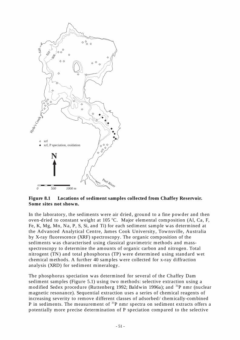
- 51 -

xrfxrf, P speciation, oxidation

0 500 1000 m

51051

8

506

N

Peel River

Hyd

e’s C

reek

Figure 8.1 Locations of sediment samples collected from Chaffey Reservoir.Some sites not shown.

In the laboratory, the sediments were air dried, ground to a fine powder and thenoven-dried to constant weight at 105 oC. Major elemental composition (Al, Ca, F,Fe, K, Mg, Mn, Na, P, S, Si, and Ti) for each sediment sample was determined atthe Advanced Analytical Centre, James Cook University, Townsville, Australiaby X-ray fluorescence (XRF) spectroscopy. The organic composition of thesediments was characterised using classical gravimetric methods and mass-spectroscopy to determine the amounts of organic carbon and nitrogen. Totalnitrogent (TN) and total phosphorus (TP) were determined using standard wetchemical methods. A further 40 samples were collected for x-ray diffractionanalysis (XRD) for sediment mineralogy.

The phosphorus speciation was determined for several of the Chaffey Damsediment samples (Figure 5.1) using two methods: selective extraction using amodified Sedex procedure (Ruttenberg 1992; Baldwin 1996a); and 31P nmr (nuclearmagnetic resonance). Sequential extraction uses a series of chemical reagents ofincreasing severity to remove different classes of adsorbed/chemically-combinedP in sediments. The measurement of 31P nmr spectra on sediment extracts offers apotentially more precise determination of P speciation compared to the selective

- 52 -

extraction method. In the nmr method, approximately 20 g of sediment wasextracted into 10 mL of 0.5 M NaOH. Following extraction approximately 1 g ofChelex resin was added to the extractant, which was then allowed to sit overnightprior to filtering. 31P nmr spectra of the extractants were obtained by Dr MaxKinery, ANU.

8.2.2 Reservoir siltation

The low storage level in February 1995 allowed us to visit two of the silt padslocated in the southern basins (Figure 5.1) that were installed when the dam wasconstructed. The silt pads are 6 m x 6 m concrete blocks poured so that theirsurface was level with the surrounding ground prior to the initial inundation ofthe reservoir. They serve as a reference level for measuring the siltation rate ofthe dam. The pad in the central basin had an average of 11 cm of dry sediment onit, indicating an average siltation rate of 8 mm per annum. This is a value local tothe silt pad and does not necessarily reflect a basin-wide average. However,measurement at another silt pad on the opposite side of the river channelconfirmed this value. Further confirmation is provided by the sediment core datapresented in section 8.2.4.

8.2.3 Elemental and mineralogical composition of the sediments

Baldwin et al. (1998) used a variety of non-parametric statistical techniques(Multi-Dimensional Scaling (MDS), Analysis of Similarity (ANOSIM) andSimilarity Percentages (SIMPER)) to analyse the XRF elemental composition dataand define the spatial variability of sediment composition within the reservoirand between Dungowan and Chaffey reservoirs. The analysis showed threegroups of sediments were present: the Peel R. floodplain sediments, Hyde Ck.floodplain sediments, and the sediments in the main basin. The results wereconsistent with the findings of Caitcheon et al. (1994) and Donnelly (1993) that themajority of the sediment is derived from the Tertiary basalts in the easterncatchment.

The geographical grouping of sediments is not surprising as the sediments carriedby the Peel R. and Hyde Ck. have significantly different origins (Tertiary basalt vsDevonian sediment) and the coarser particles sediment out preferentially in theflood plains close to where the streams enter the reservoir. The main basinsediments contain a relatively higher content of fine particles due to sedimentfocusing. Sediment focusing refers to the resuspension of fine particles (clay,containing more aluminium) from the periphery of a reservoir which aresubsequently deposited in the deeper portions of the dam. The sands, whichcontain more silica, are left behind.

Semi-quantitative XRD analysis detected four minerals in the sediments:smectite, quartz, plagioclase, and kaolinite. Smectite was dominant, with thethree remaining minerals being present in accessory (5-20%) or trace components(<5%). The variation of concentration of phosphorus in the sediment wasstrongly correlated (r2 = 0.98) with iron, manganese, and magnesium in thesediment. There was no correlation between the sedimentary phosphorusconcentration and particle size, nor with total organic carbon.

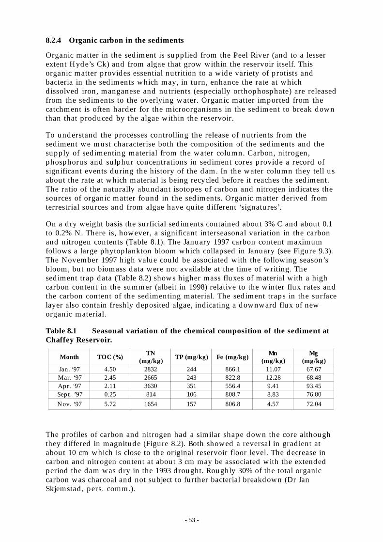
- 53 -

8.2.4 Organic carbon in the sediments

Organic matter in the sediment is supplied from the Peel River (and to a lesserextent Hyde’s Ck) and from algae that grow within the reservoir itself. Thisorganic matter provides essential nutrition to a wide variety of protists andbacteria in the sediments which may, in turn, enhance the rate at whichdissolved iron, manganese and nutrients (especially orthophosphate) are releasedfrom the sediments to the overlying water. Organic matter imported from thecatchment is often harder for the microorganisms in the sediment to break downthan that produced by the algae within the reservoir.

To understand the processes controlling the release of nutrients from thesediment we must characterise both the composition of the sediments and thesupply of sedimenting material from the water column. Carbon, nitrogen,phosphorus and sulphur concentrations in sediment cores provide a record ofsignificant events during the history of the dam. In the water column they tell usabout the rate at which material is being recycled before it reaches the sediment.The ratio of the naturally abundant isotopes of carbon and nitrogen indicates thesources of organic matter found in the sediments. Organic matter derived fromterrestrial sources and from algae have quite different ‘signatures’.

On a dry weight basis the surficial sediments contained about 3% C and about 0.1to 0.2% N. There is, however, a significant interseasonal variation in the carbonand nitrogen contents (Table 8.1). The January 1997 carbon content maximumfollows a large phytoplankton bloom which collapsed in January (see Figure 9.3).The November 1997 high value could be associated with the following season’sbloom, but no biomass data were not available at the time of writing. Thesediment trap data (Table 8.2) shows higher mass fluxes of material with a highcarbon content in the summer (albeit in 1998) relative to the winter flux rates andthe carbon content of the sedimenting material. The sediment traps in the surfacelayer also contain freshly deposited algae, indicating a downward flux of neworganic material.

Table 8.1 Seasonal variation of the chemical composition of the sediment atChaffey Reservoir.

Month TOC (%)TN

(mg/kg)TP (mg/kg) Fe (mg/kg)

Mn(mg/kg)

Mg(mg/kg)

Jan. ‘97 4.50 2832 244 866.1 11.07 67.67Mar. ‘97 2.45 2665 243 822.8 12.28 68.48Apr. ‘97 2.11 3630 351 556.4 9.41 93.45Sept. ’97 0.25 814 106 808.7 8.83 76.80Nov. ‘97 5.72 1654 157 806.8 4.57 72.04

The profiles of carbon and nitrogen had a similar shape down the core althoughthey differed in magnitude (Figure 8.2). Both showed a reversal in gradient atabout 10 cm which is close to the original reservoir floor level. The decrease incarbon and nitrogen content at about 3 cm may be associated with the extendedperiod the dam was dry in the 1993 drought. Roughly 30% of the total organiccarbon was charcoal and not subject to further bacterial breakdown (Dr JanSkjemstad, pers. comm.).

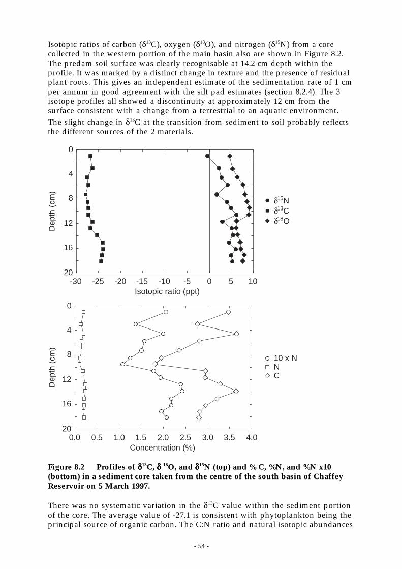
- 54 -

Isotopic ratios of carbon (δ13C), oxygen (δ18O), and nitrogen (δ15N) from a corecollected in the western portion of the main basin also are shown in Figure 8.2.The predam soil surface was clearly recognisable at 14.2 cm depth within theprofile. It was marked by a distinct change in texture and the presence of residualplant roots. This gives an independent estimate of the sedimentation rate of 1 cmper annum in good agreement with the silt pad estimates (section 8.2.4). The 3isotope profiles all showed a discontinuity at approximately 12 cm from thesurface consistent with a change from a terrestrial to an aquatic environment.The slight change in δ13C at the transition from sediment to soil probably reflectsthe different sources of the 2 materials.

-30 -25 -20 -15 -10 -5 0 5 10

0

4

8

12

16

20

Isotopic ratio (ppt)

0.0 0.5 1.0 1.5 2.0 2.5 3.0 3.5 4.0

0

4

8

12

16

20

Concentration (%)

Dep

th (

cm)

Dep

th (

cm)

10 x NNC

δ18Oδ13Cδ15N

Figure 8.2 Profiles of δδδδ13C, δδδδ 18O, and δδδδ15N (top) and % C, %N, and %N x10(bottom) in a sediment core taken from the centre of the south basin of ChaffeyReservoir on 5 March 1997.

There was no systematic variation in the δ13C value within the sediment portionof the core. The average value of -27.1 is consistent with phytoplankton being theprincipal source of organic carbon. The C:N ratio and natural isotopic abundances

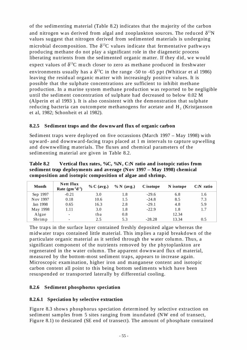
- 55 -

of the sedimenting material (Table 8.2) indicates that the majority of the carbonand nitrogen was derived from algal and zooplankton sources. The reduced δ15Nvalues suggest that nitrogen derived from sedimented materials is undergoingmicrobial decomposition. The δ13C values indicate that fermentative pathwaysproducing methane do not play a significant role in the diagenetic processliberating nutrients from the sedimented organic matter. If they did, we wouldexpect values of δ13C much closer to zero as methane produced in freshwaterenvironments usually has a δ13C in the range -50 to -65 ppt (Whiticar et al 1986)leaving the residual organic matter with increasingly positive values. It ispossible that the sulphate concentrations are sufficient to inhibit methaneproduction. In a marine system methane production was reported to be negligibleuntil the sediment concentration of sulphate had decreased to below 0.02 M(Alperin et al 1993 ). It is also consistent with the demonstration that sulphatereducing bacteria can outcompete methanogens for acetate and H2 (Kristjanssonet al, 1982; Schonheit et al 1982).

8.2.5 Sediment traps and the downward flux of organic carbon

Sediment traps were deployed on five occassions (March 1997 – May 1998) withupward- and downward-facing traps placed at 1 m intervals to capture upwellingand downwelling materials. The fluxes and chemical parameters of thesedimenting material are given in Table 8.2.

Table 8.2 Vertical flux rates, %C, %N, C:N ratio and isotopic ratios fromsediment trap deployments and average (Nov 1997 – May 1998) chemicalcomposition and isotopic composition of algae and shrimp.

MonthNett Flux

Rate (gm-2d-1)% C (avg.) % N (avg.) C isotope N isotope C:N ratio

Sep 1997 -0.21 3.0 1.8 -29.6 6.8 1.6Nov 1997 0.18 10.6 1.5 -24.8 8.5 7.3Jan 1998 0.65 16.3 2.8 -29.1 4.8 5.9

May 1998 1.11 3.0 1.8 -22.9 1.8 1.7Algae - tba 0.8 12.34

Shrimp - 2.5 5.3 -28.28 13.34 0.5

The traps in the surface layer contained freshly deposited algae whereas themidwater traps contained little material. This implies a rapid breakdown of theparticulate organic material as it settled through the water column. Thus, asignificant component of the nutrients removed by the phytoplankton areregenerated in the water column. The apparent downward flux of material,measured by the bottom-most sediment traps, appears to increase again.Microscopic examination, higher iron and manganese content and isotopiccarbon content all point to this being bottom sediments which have beenresuspended or transported laterally by differential cooling.

8.2.6 Sediment phosphorus speciation

8.2.6.1 Speciation by selective extraction

Figure 8.3 shows phosphorus speciation determined by selective extraction onsediment samples from 5 sites ranging from inundated (NW end of transect,Figure 8.1) to desicated (SE end of transect). The amount of phosphate contained

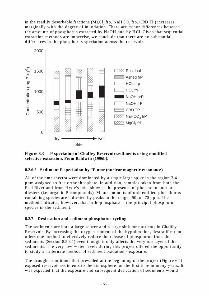
- 56 -

in the readily desorbable fractions (MgCl2 frp, NaHCO3 frp, CBD TP) increasesmarginally with the degree of inundation. There are minor differences betweenthe amounts of phosphorus extracted by NaOH and by HCl. Given that sequentialextraction methods are imprecise, we conclude that there are no substantialdifferences in the phosphorus speciation across the reservoir.

Con

cent

ratio

n (m

g P

kg-1

)

2000

1500

1000

500

0

dry wetSite

Residual

Ashed frP

HCL nrp

HCL frP

NaOH nrP

NaOH frP

CBD TP

NaHCO3 frP

MgCl2 frP

Figure 8.3 P-speciation of Chaffey Reservoir sediments using modifiedselective extraction. From Baldwin (1996b).

8.2.6.2 Sediment P speciation by 31P nmr (nuclear magnetic resonance)

All of the nmr spectra were dominated by a single large spike in the region 3-4ppm assigned to free orthophosphate. In addition, samples taken from both thePeel River and from Hyde’s inlet showed the presence of phosmono and/ordiesters (i.e. organic P compounds). Minor amounts of unidentified phosphoruscontaining species are indicated by peaks in the range –50 to –70 ppm. Themethod indicates, however, that orthophosphate is the principal phosphorusspecies in the sediment.

8.2.7 Desiccation and sediment phosphorus cycling

The sediments are both a large source and a large sink for nutrients in ChaffeyReservoir. By increasing the oxygen content of the hypolimnion, destratificationoffers one method to effectively reduce the release of phosphorus from thesediments (Section 8.5.3.1) even though it only affects the very top layer of thesediments. The very low water levels during this project offered the opportunityto study an alternate method of sediment oxidation - exposure.

The drought conditions that prevailed at the beginning of the project (Figure 6.4)exposed reservoir sediments to the atmosphere for the first time in many years. Itwas expected that the exposure and subsequent desiccation of sediments would

- 57 -

greatly affect both the abiotic (e.g. mineralogical) and biotic (particularlymicrobial) components of the sediment and, consequently, should have aprofound effect on the nutrient dynamics in the sediments. Here we report onthe effects of desiccation/oxidation on the sediment’s capacity to adsorb P underoxic conditions (analogous to a flood event); and the effects of drying on thepotential for sediments to release P under anaerobic conditions.

8.2.7.1 The effects of desiccation/oxidation on the sediment’s capacity to adsorb Punder oxic conditions

Most of the external nutrient load entering into the dam occurs during floodevents (Section 8.5.1). Although much of these nutrients are associated withparticles, a significant amount are dissolved in the (oxic) floodwaters andpotentially may be adsorbed by reservoir sediments.

The capacity of sediments of varying oxic status to adsorb inflowing dissolvedphosphorus was studied by taking 11 sediment samples along a transect (Figure5.1) which covered heavily desiccated, wet-littoral and submerged sedimentsfrom both above and below the oxycline and measuring P adsorption isotherms(Baldwin 1996b). The isotherm experiments showed a clear transition in P affinityalong the transect; sediments taken from the driest sites had the least adsorptivecapacity, those from the wet littoral regions had an intermediate capacity toadsorb P while sediments taken from beneath the oxycline had the highestaffinity for P. Also, the rate of P uptake was faster from sediments which wereinitially anoxic than from wet littoral or desiccated sediments. The differences inP affinity are believed to be a consequence of increasing crystallinity as a functionof aging (Baldwin 1996b).

Figure 8.4 shows a conceptual model of Fe cycling under oxic/anoxic conditions -the so called ‘ferrous’ wheel. Fe(III) is reduced under anoxic conditions to giveFe(II). Fe(II) is subsequently oxidised under oxic conditions to give Fe(III) - usuallyforming amorphous iron oxyhydroxides [Fe(OOH)].

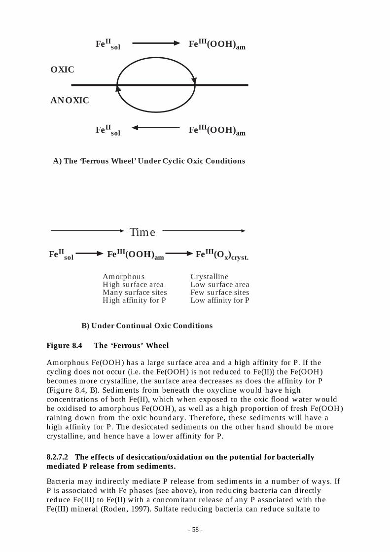
- 58 -

A) The ‘Ferrous Wheel’ Under Cyclic Oxic Conditions

B) Under Continual Oxic Conditions

Time

AmorphousHigh surface areaMany surface sitesHigh affinity for P

CrystallineLow surface areaFew surface sitesLow affinity for P

FeIIsol FeIII(OOH)am FeIII(Ox)cryst.

FeIII(OOH)amFeIIsol

FeIIsol FeIII(OOH)am

OXIC

ANOXIC

Figure 8.4 The ‘Ferrous’ Wheel

Amorphous Fe(OOH) has a large surface area and a high affinity for P. If thecycling does not occur (i.e. the Fe(OOH) is not reduced to Fe(II)) the Fe(OOH)becomes more crystalline, the surface area decreases as does the affinity for P(Figure 8.4, B). Sediments from beneath the oxycline would have highconcentrations of both Fe(II), which when exposed to the oxic flood water wouldbe oxidised to amorphous Fe(OOH), as well as a high proportion of fresh Fe(OOH)raining down from the oxic boundary. Therefore, these sediments will have ahigh affinity for P. The desiccated sediments on the other hand should be morecrystalline, and hence have a lower affinity for P.

8.2.7.2 The effects of desiccation/oxidation on the potential for bacteriallymediated P release from sediments.

Bacteria may indirectly mediate P release from sediments in a number of ways. IfP is associated with Fe phases (see above), iron reducing bacteria can directlyreduce Fe(III) to Fe(II) with a concomitant release of any P associated with theFe(III) mineral (Roden, 1997). Sulfate reducing bacteria can reduce sulfate to

- 59 -

sulfide. Sulfide is a strong enough reducing agent that it can reduce Fe(III) toFe(II) again liberating any bound P (Berner, 1984; Caraco, 1993). P may also bedirectly released from bacteria which contain poly-phosphate granules duringanaerobic respiration (Davelaar 1993, Gächter and Meyers 1993). If anaerobic Prelease is bacterially mediated, then oxidation/desiccation of sediments shouldlead to a significant change in the sedimentary bacterial community structure andhence, sedimentary P cycling.

To examine this possibility, sediments were taken from 4 sites in the reservoir,two sites which had remained inundated and were covered by anoxic waters, onewhich had recently been inundated after a prolonged period of exposure and, onewhich had yet to be inundated. Sediment samples from the four sites wereslurried under anaerobic conditions in the presence of a toxicant ( formaldehyde),various carbon sources (glucose or acetate), an electron acceptor (sulfate), or withno additional augmentation (Mitchell and Baldwin 1997).

In the absence of any augmentation, the sediments from the two sites which werenot desiccated released significant quantities of P under anaerobic conditions,while the sediments from the two sites which were desiccated showed nosignificant P release - clearly indicating that anaerobic P release can besubstantially reduced as a consequence of desiccation/oxidation. No P releaseoccurred from sediments from the two wet sites if the sediments were poisonedwith formaldehyde - indicating that P release was indeed bacterially mediated.Further evidence for bacterial mediation was the enhancement of P release fromthe wet sites when carbon (in the form of acetate), an electron acceptor (sulfate) orboth were added to the slurries. P was released from the desiccated sedimentswhen additional carbon was added, suggesting that P release from desiccatedsediments may be carbon limited, but no additional P release was observed whensulfate was added indicating that, unlike the wet sediments, sulfate reduction wasnot occurring.

Exposure of sediments to the atmosphere and subsequent desiccation has aprofound effect on sedimentary nutrient cycling. Depending on how much timeis required for bacteria to recolonize recently inundated sediments, sedimentdessication may provide a useful tool for changing the sediment chemistry ofreservoirs.

8.3 Water column chemistry

8.3.1 Methods

Routine measurement of water column chemistry (cations, anions, nitrogen,phosphorus and silica) at Chaffey Reservoir commenced in 1979. The samplingeffort was most intense during 1988-1993 and 1995-1997 and the number ofanalytes determined varied from year to year. Prior to the commencement of thisproject in mid-1995 samples were typically collected by DLWC at Stn 1 (Figure 5.1)from the surface layer (typically ca. 25 cm depth) and from 1 m above the bottom.On some occasions an additional sample was collected at mid-depth. Thefrequency of sampling was typically fortnightly, although it varied from weekly tomontly. As well, samples were collected occasionally at Stn 2 and Stn 3 and atseveral other sites including the Peel River and some of its tributaries duringperiods of more intensive monitoring. Full depth profiles (1-2 m intervals) were

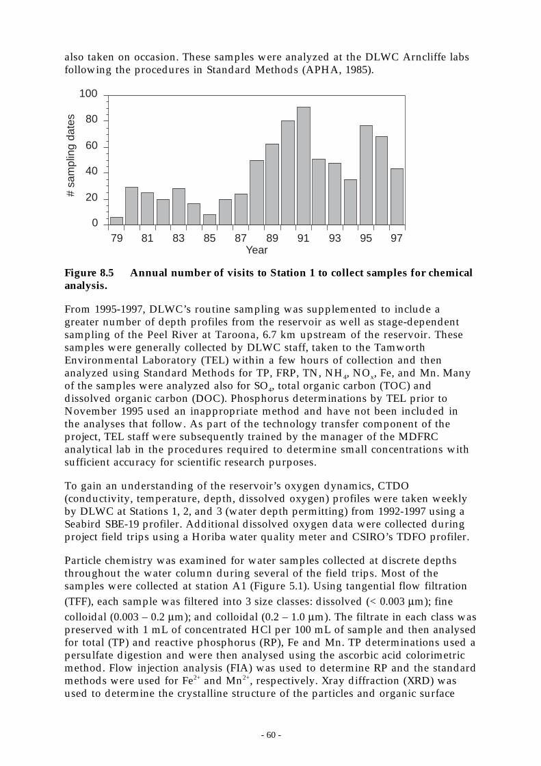
- 60 -

also taken on occasion. These samples were analyzed at the DLWC Arncliffe labsfollowing the procedures in Standard Methods (APHA, 1985).

0

20

40

60

80

100

79 81 83 85 87 89 91 93 95 97Year

# sa

mpl

ing

date

s

Figure 8.5 Annual number of visits to Station 1 to collect samples for chemicalanalysis.

From 1995-1997, DLWC’s routine sampling was supplemented to include agreater number of depth profiles from the reservoir as well as stage-dependentsampling of the Peel River at Taroona, 6.7 km upstream of the reservoir. Thesesamples were generally collected by DLWC staff, taken to the TamworthEnvironmental Laboratory (TEL) within a few hours of collection and thenanalyzed using Standard Methods for TP, FRP, TN, NH4, NOx, Fe, and Mn. Manyof the samples were analyzed also for SO4, total organic carbon (TOC) anddissolved organic carbon (DOC). Phosphorus determinations by TEL prior toNovember 1995 used an inappropriate method and have not been included inthe analyses that follow. As part of the technology transfer component of theproject, TEL staff were subsequently trained by the manager of the MDFRCanalytical lab in the procedures required to determine small concentrations withsufficient accuracy for scientific research purposes.

To gain an understanding of the reservoir’s oxygen dynamics, CTDO(conductivity, temperature, depth, dissolved oxygen) profiles were taken weeklyby DLWC at Stations 1, 2, and 3 (water depth permitting) from 1992-1997 using aSeabird SBE-19 profiler. Additional dissolved oxygen data were collected duringproject field trips using a Horiba water quality meter and CSIRO’s TDFO profiler.

Particle chemistry was examined for water samples collected at discrete depthsthroughout the water column during several of the field trips. Most of thesamples were collected at station A1 (Figure 5.1). Using tangential flow filtration(TFF), each sample was filtered into 3 size classes: dissolved (< 0.003 µm); finecolloidal (0.003 – 0.2 µm); and colloidal (0.2 – 1.0 µm). The filtrate in each class waspreserved with 1 mL of concentrated HCl per 100 mL of sample and then analysedfor total (TP) and reactive phosphorus (RP), Fe and Mn. TP determinations used apersulfate digestion and were then analysed using the ascorbic acid colorimetricmethod. Flow injection analysis (FIA) was used to determine RP and the standardmethods were used for Fe2+ and Mn2+, respectively. Xray diffraction (XRD) wasused to determine the crystalline structure of the particles and organic surface

- 61 -

coatings were studied using sedimentation field-flow fractionation (SdFFF)coupled with inductively-coupled plasma mass spectroscopy (ICP-MS).

Reactive phosphorus that has passed a 0.003 µm filter is referred to in this reportas FRP0.003, to avoid confusion with the conventional use of the term FRP whichimplies passage through an 0.45 µm filter. We believe FRP0.003 is a good surrogatefor orthophosphate, but it is possible for other small chain phosphate moleculesto pass the 0.003 µm filter.

Phosphorus and dissolved organic matter (DOM) speciation were alsodetermined by weak anion exchange chromatography.

8.3.2 Historical trends in water chemistry

To understand the seasonal patterns in nutrient concentrations, it is useful toconsider individually the three classic regions of the water column: the epi-,meta- and hypo-limnia. At Chaffey Dam we have used our knowledge of thesurface layer dynamics (Figure 7.3) and oxygen profiles to define these 3 regions asoccupying the water column from 0 - 5 m, 5 - 12 m, and below 12 m, respectively.The surface layer (epilimnion) is where virtually all algal growth occurs. Thehypolimnion best reflects the sediment-water exchanges and the metalimnion isa relatively quiescent stratified region through which both particulate matterrains down from above and dissolved nutrients are transported upwards byturbulent diffusion and large scale circulation (Section 7.6).

It is important to bear in mind that the volume of the hypolimnion varies fromyear to year depending on how full the reservoir is. For a given nutrient fluxfrom the sediment to the water column, the resultant hypolimneticconcentration will increase with decreasing water level. In other words,differences in the annual maximum hypolimnetic nutrient concentrations donot necessarily imply differences in the sediment nutrient release rates.

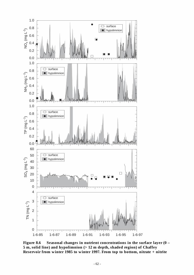
- 62 -

hypolimnionsurface

NH

3 (m

g L-1

)

0.0

0.2

0.4

0.6

0.8

1.0

0

10

20

30

40

50

60

hypolimnionsurface

SO

4 (m

g L-1

)

1-6-85 1-6-87 1-6-89 1-6-91 1-6-93 1-6-95 1-6-97

0

1

2

3

4

TN

(m

g L-1

) hypolimnionsurface

hypolimnionsurface

TP

(m

g L-1

)

0.0

0.2

0.4

0.6

0.8

1.0

hypolimnionsurface

NO

x (m

g L-1

)

0.0

0.2

0.4

0.6

0.8

1.0

Figure 8.6 Seasonal changes in nutrient concentrations in the surface layer (0 –5 m, solid line) and hypolimnion (> 12 m depth, shaded region) of ChaffeyReservoir from winter 1985 to winter 1997. From top to bottom, nitrate + nitrite

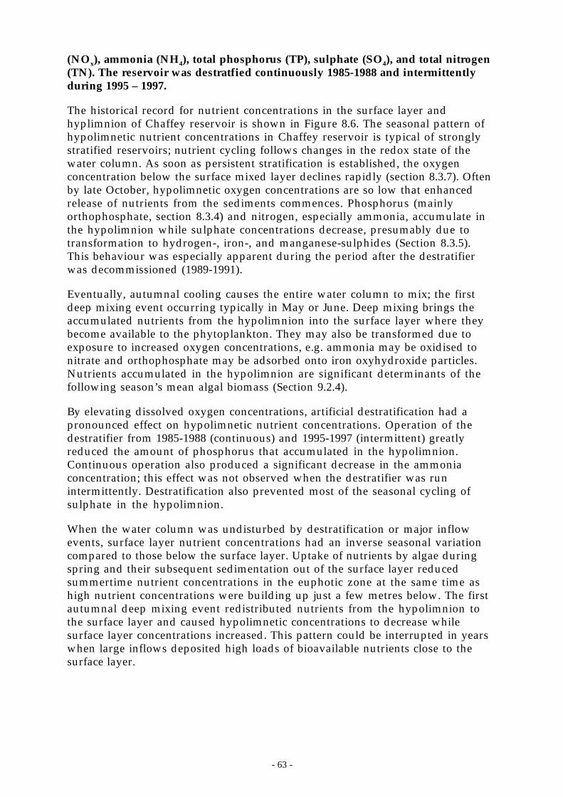
- 63 -

(NOx), ammonia (NH4), total phosphorus (TP), sulphate (SO4), and total nitrogen(TN). The reservoir was destratfied continuously 1985-1988 and intermittentlyduring 1995 – 1997.

The historical record for nutrient concentrations in the surface layer andhyplimnion of Chaffey reservoir is shown in Figure 8.6. The seasonal pattern ofhypolimnetic nutrient concentrations in Chaffey reservoir is typical of stronglystratified reservoirs; nutrient cycling follows changes in the redox state of thewater column. As soon as persistent stratification is established, the oxygenconcentration below the surface mixed layer declines rapidly (section 8.3.7). Oftenby late October, hypolimnetic oxygen concentrations are so low that enhancedrelease of nutrients from the sediments commences. Phosphorus (mainlyorthophosphate, section 8.3.4) and nitrogen, especially ammonia, accumulate inthe hypolimnion while sulphate concentrations decrease, presumably due totransformation to hydrogen-, iron-, and manganese-sulphides (Section 8.3.5).This behaviour was especially apparent during the period after the destratifierwas decommissioned (1989-1991).

Eventually, autumnal cooling causes the entire water column to mix; the firstdeep mixing event occurring typically in May or June. Deep mixing brings theaccumulated nutrients from the hypolimnion into the surface layer where theybecome available to the phytoplankton. They may also be transformed due toexposure to increased oxygen concentrations, e.g. ammonia may be oxidised tonitrate and orthophosphate may be adsorbed onto iron oxyhydroxide particles.Nutrients accumulated in the hypolimnion are significant determinants of thefollowing season’s mean algal biomass (Section 9.2.4).

By elevating dissolved oxygen concentrations, artificial destratification had apronounced effect on hypolimnetic nutrient concentrations. Operation of thedestratifier from 1985-1988 (continuous) and 1995-1997 (intermittent) greatlyreduced the amount of phosphorus that accumulated in the hypolimnion.Continuous operation also produced a significant decrease in the ammoniaconcentration; this effect was not observed when the destratifier was runintermittently. Destratification also prevented most of the seasonal cycling ofsulphate in the hypolimnion.

When the water column was undisturbed by destratification or major inflowevents, surface layer nutrient concentrations had an inverse seasonal variationcompared to those below the surface layer. Uptake of nutrients by algae duringspring and their subsequent sedimentation out of the surface layer reducedsummertime nutrient concentrations in the euphotic zone at the same time ashigh nutrient concentrations were building up just a few metres below. The firstautumnal deep mixing event redistributed nutrients from the hypolimnion tothe surface layer and caused hypolimnetic concentrations to decrease whilesurface layer concentrations increased. This pattern could be interrupted in yearswhen large inflows deposited high loads of bioavailable nutrients close to thesurface layer.

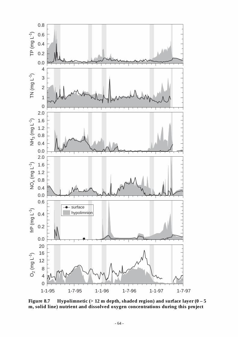
- 64 -

TP

(m

g L-1

)T

N (

mg

L-1)

NH

3 (m

g L-1

)N

Ox

(mg

L-1)

frP

(m

g L-1

)

0.0

0.2

0.4

0.6

0.8

0

1

2

3

4

0.0

0.4

0.8

1.2

1.6

2.0

0.0

0.4

0.8

1.2

1.6

2.0

0.0

0.2

0.4

0.6

hypolimnionsurface

O2

(mg

L-1)

0

4

8

12

1620

1-7-971-1-95 1-7-95 1-1-96 1-7-96 1-1-97

Figure 8.7 Hypolimnetic (> 12 m depth, shaded region) and surface layer (0 – 5m, solid line) nutrient and dissolved oxygen concentrations during this project

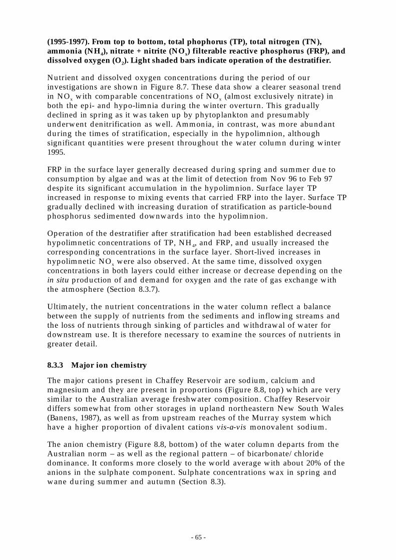
- 65 -

(1995-1997). From top to bottom, total phophorus (TP), total nitrogen (TN),ammonia (NH4), nitrate + nitrite (NOx) filterable reactive phosphorus (FRP), anddissolved oxygen (O2). Light shaded bars indicate operation of the destratifier.

Nutrient and dissolved oxygen concentrations during the period of ourinvestigations are shown in Figure 8.7. These data show a clearer seasonal trendin NOx with comparable concentrations of NOx (almost exclusively nitrate) inboth the epi- and hypo-limnia during the winter overturn. This graduallydeclined in spring as it was taken up by phytoplankton and presumablyunderwent denitrification as well. Ammonia, in contrast, was more abundantduring the times of stratification, especially in the hypolimnion, althoughsignificant quantities were present throughout the water column during winter1995.

FRP in the surface layer generally decreased during spring and summer due toconsumption by algae and was at the limit of detection from Nov 96 to Feb 97despite its significant accumulation in the hypolimnion. Surface layer TPincreased in response to mixing events that carried FRP into the layer. Surface TPgradually declined with increasing duration of stratification as particle-boundphosphorus sedimented downwards into the hypolimnion.

Operation of the destratifier after stratification had been established decreasedhypolimnetic concentrations of TP, NH4, and FRP, and usually increased thecorresponding concentrations in the surface layer. Short-lived increases inhypolimnetic NOx were also observed. At the same time, dissolved oxygenconcentrations in both layers could either increase or decrease depending on thein situ production of and demand for oxygen and the rate of gas exchange withthe atmosphere (Section 8.3.7).

Ultimately, the nutrient concentrations in the water column reflect a balancebetween the supply of nutrients from the sediments and inflowing streams andthe loss of nutrients through sinking of particles and withdrawal of water fordownstream use. It is therefore necessary to examine the sources of nutrients ingreater detail.

8.3.3 Major ion chemistry

The major cations present in Chaffey Reservoir are sodium, calcium andmagnesium and they are present in proportions (Figure 8.8, top) which are verysimilar to the Australian average freshwater composition. Chaffey Reservoirdiffers somewhat from other storages in upland northeastern New South Wales(Banens, 1987), as well as from upstream reaches of the Murray system whichhave a higher proportion of divalent cations vis-a-vis monovalent sodium.

The anion chemistry (Figure 8.8, bottom) of the water column departs from theAustralian norm – as well as the regional pattern – of bicarbonate/chloridedominance. It conforms more closely to the world average with about 20% of theanions in the sulphate component. Sulphate concentrations wax in spring andwane during summer and autumn (Section 8.3).

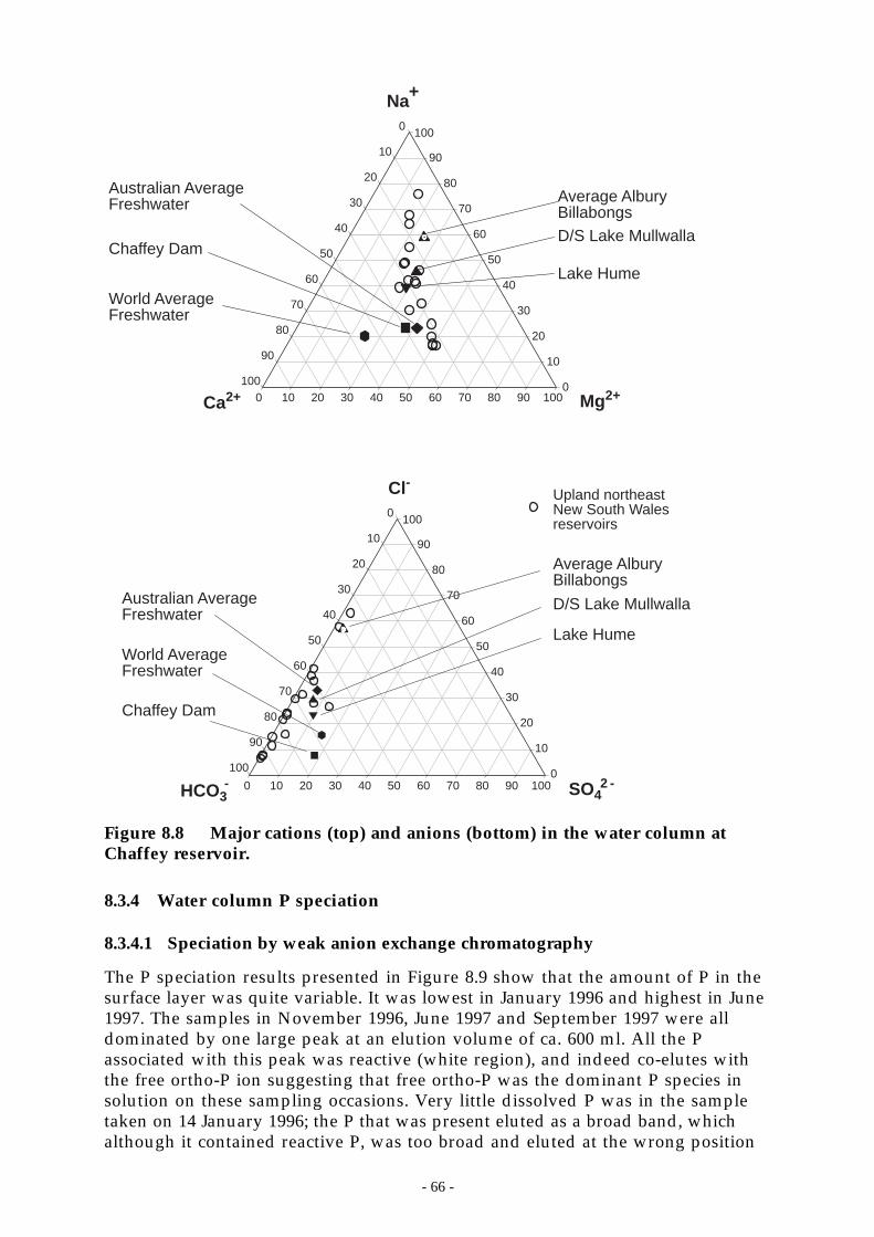
- 66 -

Mg2+

Na+

Chaffey Dam

Australian AverageFreshwater

Lake Hume

D/S Lake Mullwalla

Average AlburyBillabongs

Ca2+

World AverageFreshwater

0

10

20

30

40

50

60

70

80

90

1001000 10 20 30 40 50 60 70 80 90

0

10

20

60

70

80

90

100

30

40

50

Upland northeastNew South Walesreservoirs

SO42 -

Cl-

HCO3-

0

10

20

30

40

50

60

70

80

90

100

1000 10 20 30 40 50 60 70 80 900

10

20

60

70

80

90

100

30

40

50

Australian AverageFreshwater

Chaffey Dam

World AverageFreshwater

Average AlburyBillabongs

Lake Hume

D/S Lake Mullwalla

Figure 8.8 Major cations (top) and anions (bottom) in the water column atChaffey reservoir.

8.3.4 Water column P speciation

8.3.4.1 Speciation by weak anion exchange chromatography

The P speciation results presented in Figure 8.9 show that the amount of P in thesurface layer was quite variable. It was lowest in January 1996 and highest in June1997. The samples in November 1996, June 1997 and September 1997 were alldominated by one large peak at an elution volume of ca. 600 ml. All the Passociated with this peak was reactive (white region), and indeed co-elutes withthe free ortho-P ion suggesting that free ortho-P was the dominant P species insolution on these sampling occasions. Very little dissolved P was in the sampletaken on 14 January 1996; the P that was present eluted as a broad band, whichalthough it contained reactive P, was too broad and eluted at the wrong position

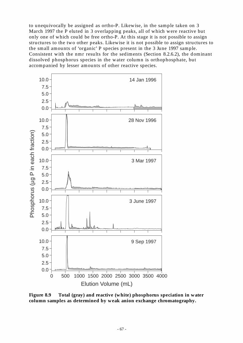
- 67 -

to unequivocally be assigned as ortho-P. Likewise, in the sample taken on 3March 1997 the P eluted in 3 overlapping peaks, all of which were reactive butonly one of which could be free ortho-P. At this stage it is not possible to assignstructures to the two other peaks. Likewise it is not possible to assign structures tothe small amounts of ‘organic’ P species present in the 3 June 1997 sample.Consistent with the nmr results for the sediments (Section 8.2.6.2), the dominantdissolved phosphorus species in the water column is orthophosphate, butaccompanied by lesser amounts of other reactive species.

10.0

7.55.0

2.50.0

10.0

7.55.0

2.50.0

10.0

7.55.0

2.50.0

10.0

7.55.0

2.50.0

10.0

7.55.0

2.50.0

Pho

spho

rus

(µg

P in

eac

h fr

actio

n)

14 Jan 1996

28 Nov 1996

3 Mar 1997

3 June 1997

9 Sep 1997

0 500 1000 1500 2000 2500 3000 3500 4000

Elution Volume (mL)

Figure 8.9 Total (gray) and reactive (white) phosphorus speciation in watercolumn samples as determined by weak anion exchange chromatography.

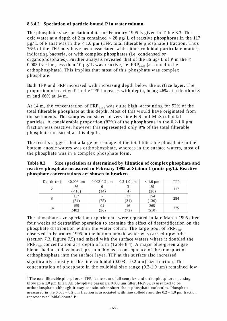
- 68 -

8.3.4.2 Speciation of particle-bound P in water column

The phosphate size speciation data for February 1995 is given in Table 8.3. Theoxic water at a depth of 2 m contained < 28 µg/L of reactive phosphorus in the 117µg/L of P that was in the < 1.0 µm (TFP, total filterable phosphate3) fraction. Thus76% of the TFP may have been associated with either colloidal particulate matter,indicating bacteria, or with complex phosphates (i.e. condensed ororganophosphates). Further analysis revealed that of the 86 µg/L of P in the <0.003 fraction, less than 10 µg/L was reactive, i.e. FRP0.003 (assumed to beorthophosphate). This implies that most of this phosphate was complexphosphate.

Both TFP and FRP increased with increasing depth below the surface layer. Theproportion of reactive P in the TFP increases with depth, being 46% at a depth of 8m and 66% at 14 m.

At 14 m, the concentration of FRP0.003 was quite high, accounting for 52% of thetotal filterable phosphate at this depth. Most of this would have originated fromthe sediments. The samples consisted of very fine FeS and MnS colloidalparticles. A considerable proportion (82%) of the phosphorus in the 0.2-1.0 µmfraction was reactive, however this represented only 9% of the total filterablephosphate measured at this depth.

The results suggest that a large percentage of the total filterable phosphate in thebottom anoxic waters was orthophosphate, whereas in the surface waters, most ofthe phosphate was in a complex phosphate form.

Table 8.3 Size speciation as determined by filtration of complex phosphate andreactive phosphate measured in February 1995 at Station 1 (units µg/L). Reactivephosphate concentrations are shown in brackets.

Depth (m) <0.003 µm 0.003-0.2 µm 0.2-1.0 µm < 1.0 µm TFP

2 86(<10)

0(14)

3(4)

89(28) 117

8 117(24)

-(75)

37(31)

154(130) 284

14 155(402)

94(36)

16(72)

265(510) 775

The phosphate size speciation experiments were repeated in late March 1995 afterfour weeks of destratifier operation to examine the effect of destratification on thephosphate distribution within the water colum. The large pool of FRP0.003

observed in February 1995 in the bottom anoxic water was carried upwards(section 7.3, Figure 7.5) and mixed with the surface waters where it doubled theFRP0.003 concentration at a depth of 2 m (Table 8.4). A major blue-green algaebloom had also developed, presumably as a consequence of the transport oforthophosphate into the surface layer. TFP at the surface also increasedsignificantly, mostly in the fine colloidal (0.003 – 0.2 µm) size fraction. Theconcentration of phosphate in the colloidal size range (0.2-1.0 µm) remained low. 3 The total filterable phosphorus, TFP, is the sum of all complex and ortho-phosphorus passingthrough a 1.0 µm filter. All phosphate passing a 0.003 µm filter, FRP0.003, is assumed to beorthophosphate although it may contain other short-chain phosphate molecules. Phosphatemeasured in the 0.003 – 0.2 µm fraction is associated with fine colloids and the 0.2 – 1.0 µm fractionrepresents colloidal-bound P.

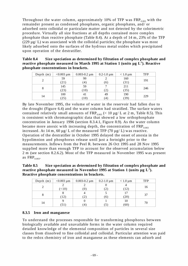
- 69 -

Throughout the water column, approximately 10% of TFP was FRP0.003 with theremainder present as condensed phosphates, organic phosphates, and/oradsorbed onto colloidal or particulate matter and not detected by the colorimetricprocedure. Virtually all size fractions at all depths contained more complexphosphate than reactive phosphate (Table 8.4). At a depth of 14 m, 23% of the TFP(229 µg/L) was associated with the colloidal particles; the phosphate was mostlikely adsorbed onto the surfaces of the hydrous metal oxides which precipitatedupon operation of the destratifier.

Table 8.4 Size speciation as determined by filtration of complex phosphate andreactive phosphate measured in March 1995 at Station 1 (units µg L-1). Reactivephosphate concentrations in brackets.

Depth (m) <0.003 µm 0.003-0.2 µm 0.2-1.0 µm < 1.0 µm TFP

2 59(21)

99(4)

2(6)

160(31) 191

8 145(23)

59(10)

7(2)

211(35) 246

14 100(25)

41(10)

49(4)

190(39) 229

By late November 1995, the volume of water in the reservoir had fallen due tothe drought (Figure 6.4) and the water column had stratified. The surface waterscontained relatively small amounts of FRP0.003 (< 10 µg/L at 2 m, Table 8.5). Thisis consistent with chromatographic data that showed a low orthophosphateconcentration in January 1996 (section 8.3.4.1, Figure 8.9). As the water columnbecame more anoxic with increasing depth, the concentration of FRP0.003

increased. At 14 m, 60 µg/L of the measured TFP (70 µg/L) was reactive.Operation of the destratifier in October 1995 delayed the onset of anoxia in thehypolimnion and phosphorus release until just a fortnight prior to themeasurements. Inflows from the Peel R. between 26 Oct 1995 and 28 Nov 1995supplied more than enough TFP to account for the observed accumulation below2 m (see section 8.2.6.2). Most of the TFP measured in November 1995 was presentas FRP0.003.

Table 8.5 Size speciation as determined by filtration of complex phosphate andreactive phosphate measured in November 1995 at Station 1 (units µg L-1).Reactive phosphate concentrations in brackets.

Depth (m) <0.003 µm 0.003-0.2 µm 0.2-1.0 µm < 1.0 µm TFP

2 2(<10)

2(0)

0(2)

4(12) 16

8 8(12)

4(2)

5(6)

17(20) 37

14 9(51)

0(4)

1(5)

10(60) 70

8.3.5 Iron and manganese

To understand the processes responsible for transforming phosphorus betweenbiologically available and unavailable forms in the water column requireddetailed knowledge of the elemental composition of particles in several sizeclasses from dissolved to fine colloidal and colloidal. Particular attention was paidto the redox chemistry of iron and manganese as these elements can adsorb and

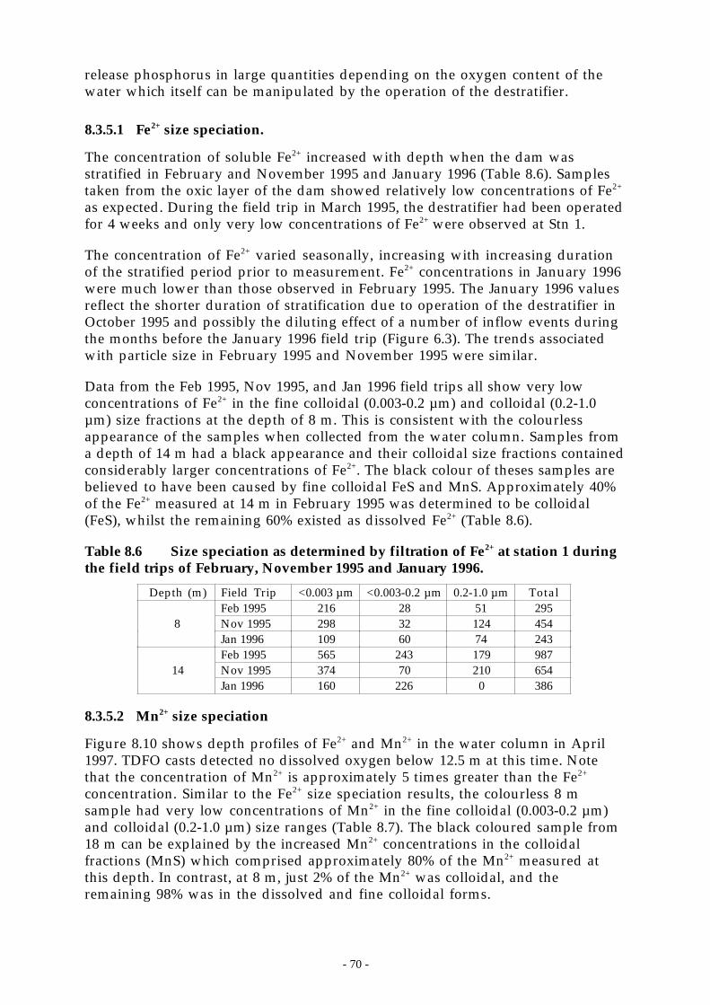
- 70 -

release phosphorus in large quantities depending on the oxygen content of thewater which itself can be manipulated by the operation of the destratifier.

8.3.5.1 Fe2+ size speciation.

The concentration of soluble Fe2+ increased with depth when the dam wasstratified in February and November 1995 and January 1996 (Table 8.6). Samplestaken from the oxic layer of the dam showed relatively low concentrations of Fe2+

as expected. During the field trip in March 1995, the destratifier had been operatedfor 4 weeks and only very low concentrations of Fe2+ were observed at Stn 1.

The concentration of Fe2+ varied seasonally, increasing with increasing durationof the stratified period prior to measurement. Fe2+ concentrations in January 1996were much lower than those observed in February 1995. The January 1996 valuesreflect the shorter duration of stratification due to operation of the destratifier inOctober 1995 and possibly the diluting effect of a number of inflow events duringthe months before the January 1996 field trip (Figure 6.3). The trends associatedwith particle size in February 1995 and November 1995 were similar.

Data from the Feb 1995, Nov 1995, and Jan 1996 field trips all show very lowconcentrations of Fe2+ in the fine colloidal (0.003-0.2 µm) and colloidal (0.2-1.0µm) size fractions at the depth of 8 m. This is consistent with the colourlessappearance of the samples when collected from the water column. Samples froma depth of 14 m had a black appearance and their colloidal size fractions containedconsiderably larger concentrations of Fe2+. The black colour of theses samples arebelieved to have been caused by fine colloidal FeS and MnS. Approximately 40%of the Fe2+ measured at 14 m in February 1995 was determined to be colloidal(FeS), whilst the remaining 60% existed as dissolved Fe2+ (Table 8.6).

Table 8.6 Size speciation as determined by filtration of Fe2+ at station 1 duringthe field trips of February, November 1995 and January 1996.

Depth (m) Field Trip <0.003 µm <0.003-0.2 µm 0.2-1.0 µm TotalFeb 1995 216 28 51 295

8 Nov 1995 298 32 124 454Jan 1996 109 60 74 243Feb 1995 565 243 179 987

14 Nov 1995 374 70 210 654Jan 1996 160 226 0 386

8.3.5.2 Mn2+ size speciation

Figure 8.10 shows depth profiles of Fe2+ and Mn2+ in the water column in April1997. TDFO casts detected no dissolved oxygen below 12.5 m at this time. Notethat the concentration of Mn2+ is approximately 5 times greater than the Fe2+

concentration. Similar to the Fe2+ size speciation results, the colourless 8 msample had very low concentrations of Mn2+ in the fine colloidal (0.003-0.2 µm)and colloidal (0.2-1.0 µm) size ranges (Table 8.7). The black coloured sample from18 m can be explained by the increased Mn2+ concentrations in the colloidalfractions (MnS) which comprised approximately 80% of the Mn2+ measured atthis depth. In contrast, at 8 m, just 2% of the Mn2+ was colloidal, and theremaining 98% was in the dissolved and fine colloidal forms.

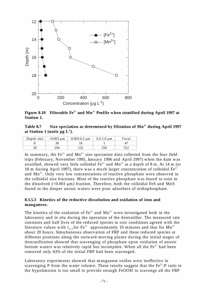
- 71 -

Concentration (µg L-1)0 200 400 600 800

[Fe2+]

[Mn2+]

12

14

16

18

20

Dep

th (

m)

Figure 8.10 Filterable Fe2+ and Mn2+ Profile when stratified during April 1997 atStation 1.

Table 8.7 Size speciation as determined by filtration of Mn2+ during April 1997at Station 1 (units µg L-1).

Depth (m) <0.003 µm 0.003-0.2 µm 0.2-1.0 µm Total8 30 16 1 4718 104 152 256 512

In summary, the Fe2+ and Mn2+ size speciation data collected from the four fieldtrips (February, November 1995, January 1996 and April 1997) when the dam wasstratified, showed very little colloidal Fe2+ and Mn2+ at a depth of 8 m. At 14 m (or18 m during April 1997), there was a much larger concentration of colloidal Fe2+

and Mn2+. Only very low concentrations of reactive phosphate were observed inthe colloidal size fractions. Most of the reactive phosphate was found to exist inthe dissolved (<0.003 µm) fraction. Therefore, both the colloidal FeS and MnSfound in the deeper anoxic waters were poor adsorbers of orthophosphate.

8.3.5.3 Kinetics of the reductive dissolution and oxidation of iron andmanganese.

The kinetics of the oxidation of Fe2+ and Mn2+ were investigated both in thelaboratory and in situ during the operation of the destratifier. The measured rateconstants and half lives of the reduced species in oxic conditions agreed with theliterature values with t1/2 for Fe2+ approximately 10 minutes and that for Mn2+

about 20 hours. Simultaneous observation of FRP and these reduced species atdifferent positions along the outward-moving plume during the initial stages ofdestratification showed that scavenging of phosphate upon oxidation of anoxicbottom waters was relatively rapid but incomplete. When all the Fe2+ had beenremoved only 63% of the initial FRP had been scavenged.

Laboratory experiments showed that manganese oxides were ineffective inscavenging P from the water column. These results suggest that the Fe2+:P ratio inthe hypolimnion is too small to provide enough FeOOH to scavenge all the FRP

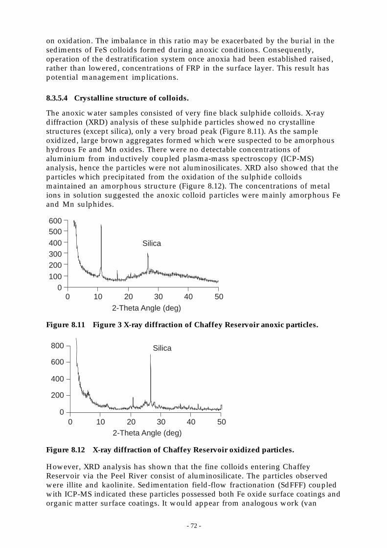
- 72 -

on oxidation. The imbalance in this ratio may be exacerbated by the burial in thesediments of FeS colloids formed during anoxic conditions. Consequently,operation of the destratification system once anoxia had been established raised,rather than lowered, concentrations of FRP in the surface layer. This result haspotential management implications.

8.3.5.4 Crystalline structure of colloids.

The anoxic water samples consisted of very fine black sulphide colloids. X-raydiffraction (XRD) analysis of these sulphide particles showed no crystallinestructures (except silica), only a very broad peak (Figure 8.11). As the sampleoxidized, large brown aggregates formed which were suspected to be amorphoushydrous Fe and Mn oxides. There were no detectable concentrations ofaluminium from inductively coupled plasma-mass spectroscopy (ICP-MS)analysis, hence the particles were not aluminosilicates. XRD also showed that theparticles which precipitated from the oxidation of the sulphide colloidsmaintained an amorphous structure (Figure 8.12). The concentrations of metalions in solution suggested the anoxic colloid particles were mainly amorphous Feand Mn sulphides.

600500

400300200

1000

2-Theta Angle (deg)

0 10 20 30 40 50

Silica

Figure 8.11 Figure 3 X-ray diffraction of Chaffey Reservoir anoxic particles.

2-Theta Angle (deg)

0

200

400

600

800

0 10 20 30 40 50

Silica

Figure 8.12 X-ray diffraction of Chaffey Reservoir oxidized particles.

However, XRD analysis has shown that the fine colloids entering ChaffeyReservoir via the Peel River consist of aluminosilicate. The particles observedwere illite and kaolinite. Sedimentation field-flow fractionation (SdFFF) coupledwith ICP-MS indicated these particles possessed both Fe oxide surface coatings andorganic matter surface coatings. It would appear from analogous work (van

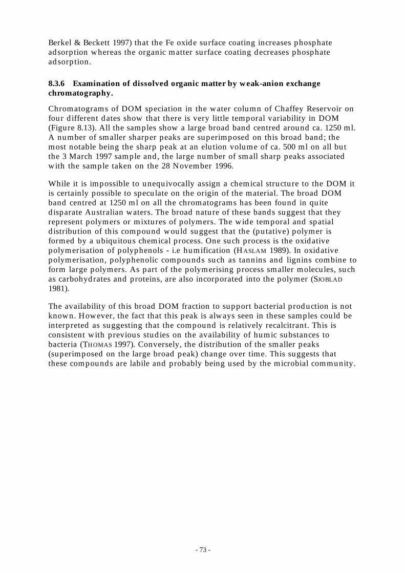
- 73 -

Berkel & Beckett 1997) that the Fe oxide surface coating increases phosphateadsorption whereas the organic matter surface coating decreases phosphateadsorption.

8.3.6 Examination of dissolved organic matter by weak-anion exchangechromatography.

Chromatograms of DOM speciation in the water column of Chaffey Reservoir onfour different dates show that there is very little temporal variability in DOM(Figure 8.13). All the samples show a large broad band centred around ca. 1250 ml.A number of smaller sharper peaks are superimposed on this broad band; themost notable being the sharp peak at an elution volume of ca. 500 ml on all butthe 3 March 1997 sample and, the large number of small sharp peaks associatedwith the sample taken on the 28 November 1996.

While it is impossible to unequivocally assign a chemical structure to the DOM itis certainly possible to speculate on the origin of the material. The broad DOMband centred at 1250 ml on all the chromatograms has been found in quitedisparate Australian waters. The broad nature of these bands suggest that theyrepresent polymers or mixtures of polymers. The wide temporal and spatialdistribution of this compound would suggest that the (putative) polymer isformed by a ubiquitous chemical process. One such process is the oxidativepolymerisation of polyphenols - i.e humification (HASLAM 1989). In oxidativepolymerisation, polyphenolic compounds such as tannins and lignins combine toform large polymers. As part of the polymerising process smaller molecules, suchas carbohydrates and proteins, are also incorporated into the polymer (SJOBLAD

1981).

The availability of this broad DOM fraction to support bacterial production is notknown. However, the fact that this peak is always seen in these samples could beinterpreted as suggesting that the compound is relatively recalcitrant. This isconsistent with previous studies on the availability of humic substances tobacteria (THOMAS 1997). Conversely, the distribution of the smaller peaks(superimposed on the large broad peak) change over time. This suggests thatthese compounds are labile and probably being used by the microbial community.

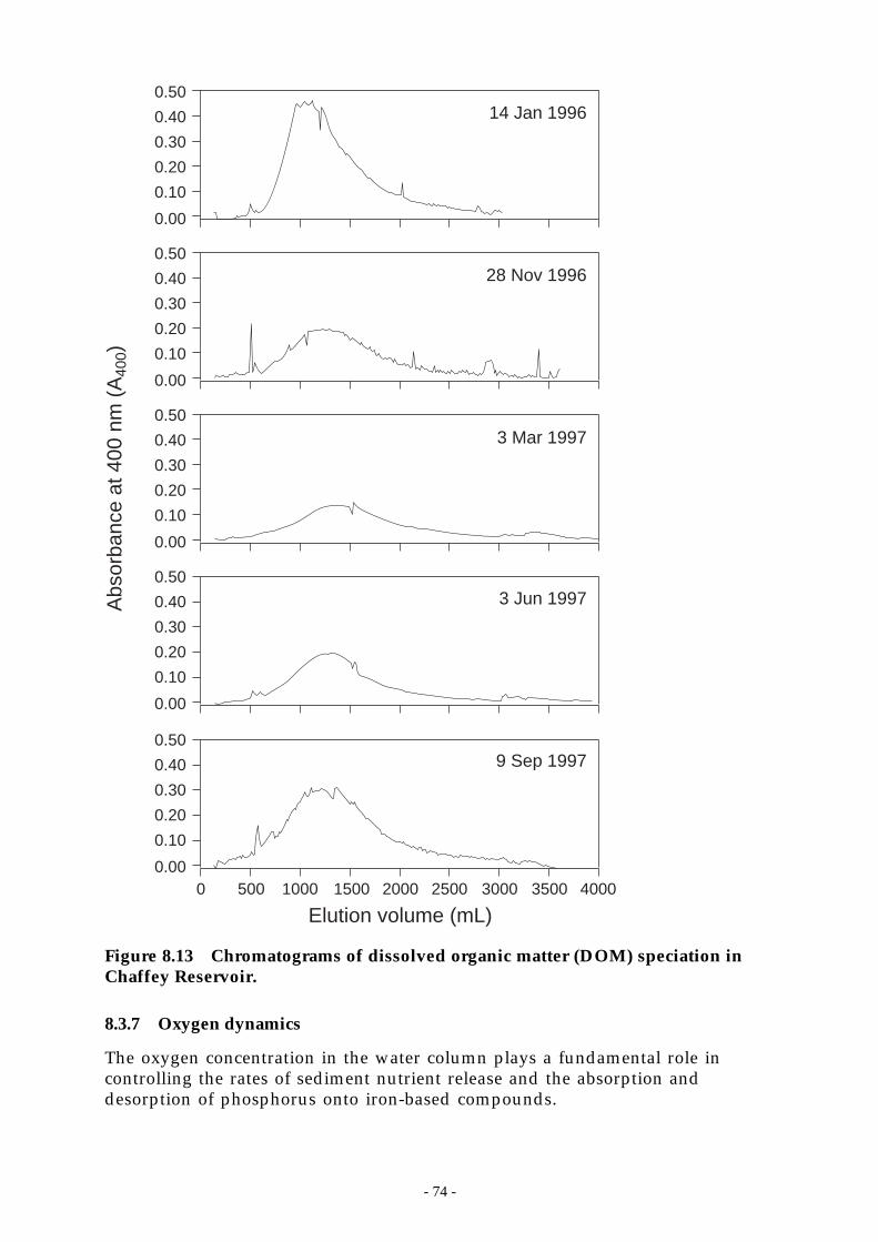
- 74 -

0 500 1000 1500 2000 2500 3500 40003000

Elution volume (mL)

0.50

0.40

0.30

0.20

0.10

0.00

0.50

0.40

0.30

0.20

0.10

0.00

0.50

0.40

0.30

0.20

0.10

0.00

0.50

0.40

0.30

0.20

0.10

0.00

0.50

0.40

0.30

0.20

0.10

0.00

Abs

orba

nce

at 4

00 n

m (

A40

0)14 Jan 1996

28 Nov 1996

3 Mar 1997

3 Jun 1997

9 Sep 1997

Figure 8.13 Chromatograms of dissolved organic matter (DOM) speciation inChaffey Reservoir.

8.3.7 Oxygen dynamics

The oxygen concentration in the water column plays a fundamental role incontrolling the rates of sediment nutrient release and the absorption anddesorption of phosphorus onto iron-based compounds.

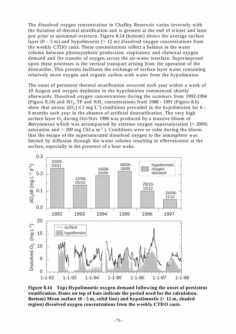
- 75 -

The dissolved oxygen concentration in Chaffey Reservoir varies inversely withthe duration of thermal stratification and is greatest at the end of winter and leastjust prior to autumnal overturn. Figure 8.14 (bottom) shows the average surfacelayer (0 – 5 m) and hypolimnetic (> 12 m) dissolved oxygen concentrations fromthe weekly CTDO casts. These concentrations reflect a balance in the watercolumn between photosynthetic production, respiratory and chemical oxygendemand and the transfer of oxygen across the air-water interface. Superimposedupon these processes is the vertical transport arising from the operation of thedestratifier. This process facilitates the exchange of surface layer water containingrelatively more oxygen and organic carbon with water from the hypolimnion.

The onset of persistent thermal stratification occurred each year within a week of10 August and oxygen depletion in the hypolimnion commenced shortlyafterwards. Dissolved oxygen concentrations during the summers from 1992-1994(Figure 8.14) and SO4, TP and NH4 concentrations from 1988 - 1991 (Figure 8.6)show that anoxic ([O2] ≤ 1 mg L-1) conditions prevailed in the hypolimnion for 6 -8 months each year in the absence of artificial destratification. The very highsurface layer O2 during Oct-Nov 1996 was produced by a massive bloom ofBotryococcus which was accompanied by extreme oxygen supersaturation (> 200%saturation and > 200 mg Chl-a m-3 ). Conditions were so calm during the bloomthat the escape of the supersaturated dissolved oxygen to the atmosphere waslimited by diffusion through the water column resulting in effervescence at thesurface, especially in the presence of a boat wake.

0

5

10

15

20

1-1-92 1-1-93 1-1-94 1-1-95 1-1-96 1-1-97 1-1-98

Dis

solv

ed O

2 (

mg

L-1)

0.0

0.1

0.2

0.3

1992 1993 1994 1995 1996 1997

dO2/

dt (

mg

L-1 d

-1)

hypolimnionsurface

hypolimneticoxygendemand

20/09 -03/11

10/08-05/10

16/08-20/09

08/08-19/09

29/10-10/12

26/08-11/11

Figure 8.14 Top) Hypolimnetic oxygen demand following the onset of persistentstratification. Dates on top of bars indicate the period used for the calculation.Bottom) Mean surface (0 - 5 m, solid line) and hypolimnetic (> 12 m, shadedregion) dissolved oxygen concentrations from the weekly CTDO casts.

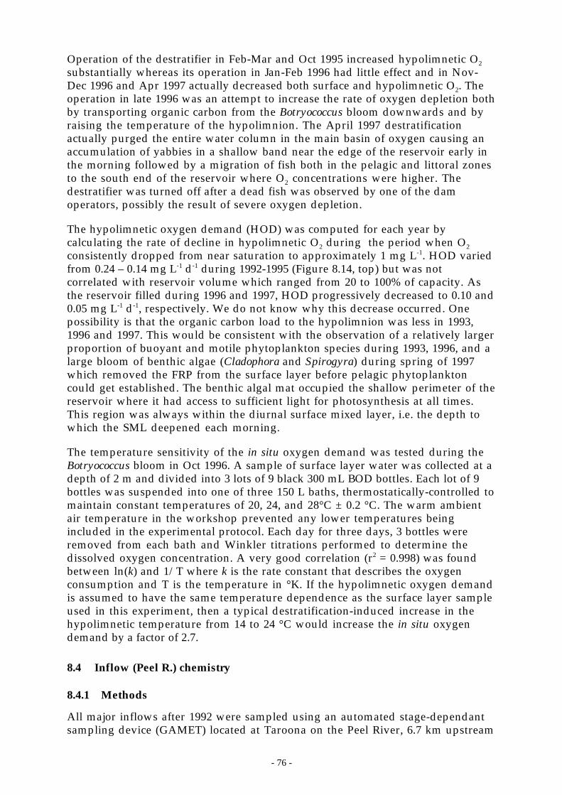
- 76 -

Operation of the destratifier in Feb-Mar and Oct 1995 increased hypolimnetic O2

substantially whereas its operation in Jan-Feb 1996 had little effect and in Nov-Dec 1996 and Apr 1997 actually decreased both surface and hypolimnetic O2. Theoperation in late 1996 was an attempt to increase the rate of oxygen depletion bothby transporting organic carbon from the Botryococcus bloom downwards and byraising the temperature of the hypolimnion. The April 1997 destratificationactually purged the entire water column in the main basin of oxygen causing anaccumulation of yabbies in a shallow band near the edge of the reservoir early inthe morning followed by a migration of fish both in the pelagic and littoral zonesto the south end of the reservoir where O2 concentrations were higher. Thedestratifier was turned off after a dead fish was observed by one of the damoperators, possibly the result of severe oxygen depletion.

The hypolimnetic oxygen demand (HOD) was computed for each year bycalculating the rate of decline in hypolimnetic O2 during the period when O2

consistently dropped from near saturation to approximately 1 mg L-1. HOD variedfrom 0.24 – 0.14 mg L-1 d-1 during 1992-1995 (Figure 8.14, top) but was notcorrelated with reservoir volume which ranged from 20 to 100% of capacity. Asthe reservoir filled during 1996 and 1997, HOD progressively decreased to 0.10 and0.05 mg L-1 d-1, respectively. We do not know why this decrease occurred. Onepossibility is that the organic carbon load to the hypolimnion was less in 1993,1996 and 1997. This would be consistent with the observation of a relatively largerproportion of buoyant and motile phytoplankton species during 1993, 1996, and alarge bloom of benthic algae (Cladophora and Spirogyra) during spring of 1997which removed the FRP from the surface layer before pelagic phytoplanktoncould get established. The benthic algal mat occupied the shallow perimeter of thereservoir where it had access to sufficient light for photosynthesis at all times.This region was always within the diurnal surface mixed layer, i.e. the depth towhich the SML deepened each morning.

The temperature sensitivity of the in situ oxygen demand was tested during theBotryococcus bloom in Oct 1996. A sample of surface layer water was collected at adepth of 2 m and divided into 3 lots of 9 black 300 mL BOD bottles. Each lot of 9bottles was suspended into one of three 150 L baths, thermostatically-controlled tomaintain constant temperatures of 20, 24, and 28°C ± 0.2 °C. The warm ambientair temperature in the workshop prevented any lower temperatures beingincluded in the experimental protocol. Each day for three days, 3 bottles wereremoved from each bath and Winkler titrations performed to determine thedissolved oxygen concentration. A very good correlation (r2 = 0.998) was foundbetween ln(k) and 1/T where k is the rate constant that describes the oxygenconsumption and T is the temperature in °K. If the hypolimnetic oxygen demandis assumed to have the same temperature dependence as the surface layer sampleused in this experiment, then a typical destratification-induced increase in thehypolimnetic temperature from 14 to 24 °C would increase the in situ oxygendemand by a factor of 2.7.

8.4 Inflow (Peel R.) chemistry

8.4.1 Methods

All major inflows after 1992 were sampled using an automated stage-dependantsampling device (GAMET) located at Taroona on the Peel River, 6.7 km upstream

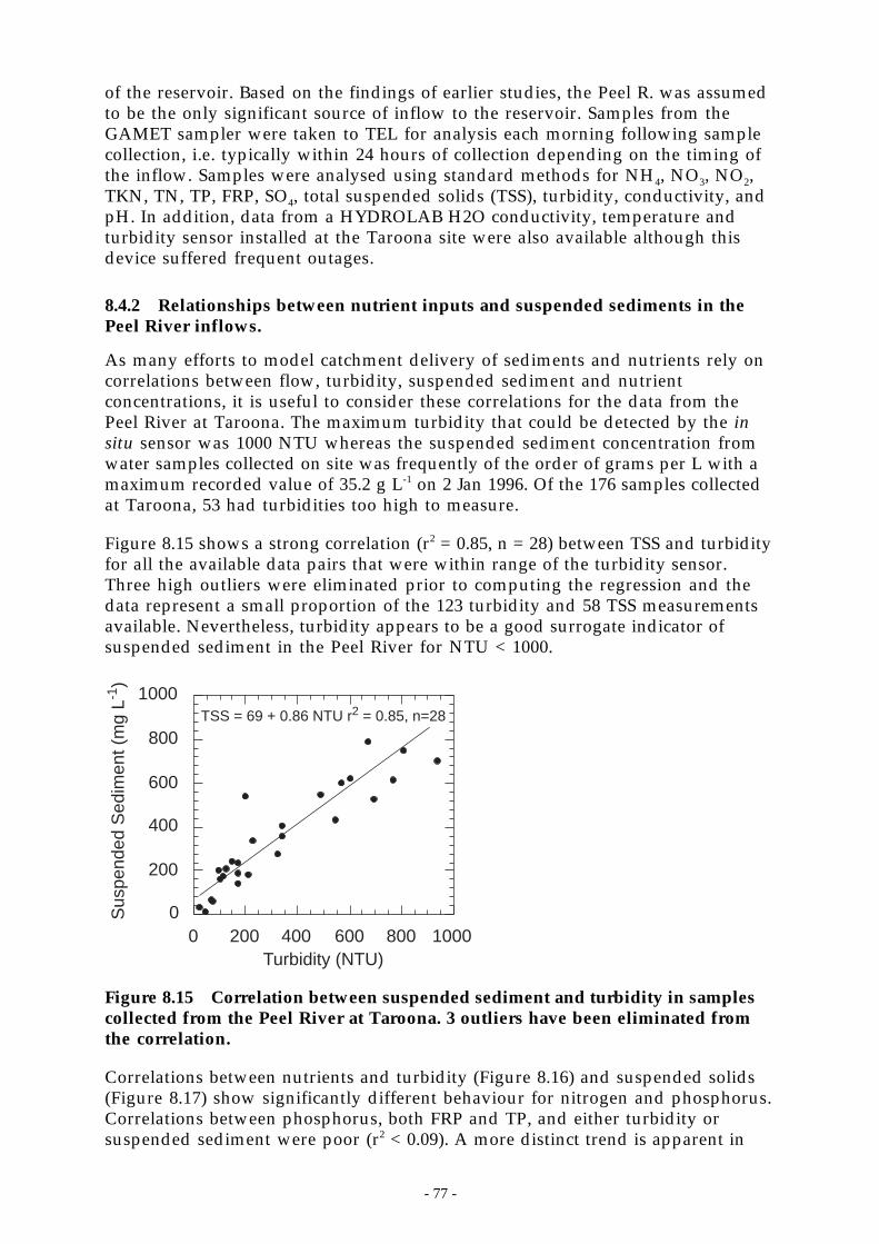
- 77 -

of the reservoir. Based on the findings of earlier studies, the Peel R. was assumedto be the only significant source of inflow to the reservoir. Samples from theGAMET sampler were taken to TEL for analysis each morning following samplecollection, i.e. typically within 24 hours of collection depending on the timing ofthe inflow. Samples were analysed using standard methods for NH4, NO3, NO2,TKN, TN, TP, FRP, SO4, total suspended solids (TSS), turbidity, conductivity, andpH. In addition, data from a HYDROLAB H2O conductivity, temperature andturbidity sensor installed at the Taroona site were also available although thisdevice suffered frequent outages.

8.4.2 Relationships between nutrient inputs and suspended sediments in thePeel River inflows.

As many efforts to model catchment delivery of sediments and nutrients rely oncorrelations between flow, turbidity, suspended sediment and nutrientconcentrations, it is useful to consider these correlations for the data from thePeel River at Taroona. The maximum turbidity that could be detected by the insitu sensor was 1000 NTU whereas the suspended sediment concentration fromwater samples collected on site was frequently of the order of grams per L with amaximum recorded value of 35.2 g L-1 on 2 Jan 1996. Of the 176 samples collectedat Taroona, 53 had turbidities too high to measure.

Figure 8.15 shows a strong correlation (r2 = 0.85, n = 28) between TSS and turbidityfor all the available data pairs that were within range of the turbidity sensor.Three high outliers were eliminated prior to computing the regression and thedata represent a small proportion of the 123 turbidity and 58 TSS measurementsavailable. Nevertheless, turbidity appears to be a good surrogate indicator ofsuspended sediment in the Peel River for NTU < 1000.

0

200

400

600

800

1000

0 200 400 600 800 1000

TSS = 69 + 0.86 NTU r2 = 0.85, n=28

Turbidity (NTU)

Sus

pend

ed S

edim

ent (

mg

L-1)

Figure 8.15 Correlation between suspended sediment and turbidity in samplescollected from the Peel River at Taroona. 3 outliers have been eliminated fromthe correlation.

Correlations between nutrients and turbidity (Figure 8.16) and suspended solids(Figure 8.17) show significantly different behaviour for nitrogen and phosphorus.Correlations between phosphorus, both FRP and TP, and either turbidity orsuspended sediment were poor (r2 < 0.09). A more distinct trend is apparent in

- 78 -

both the NOx , and TKN vs TSS data (r2 ~ 0.14 , Figure 8.17) when the highersuspended sediment concentrations (> 1000 mg L-1) are included – recall that theturbidity-based correlations are only valid to approximately 1000 mg L-1 of TSS.When individual inflow events were considered, the correlations were better (r2

> 0.6) yet distinctly different for rising and falling stages of the hydrograph andbetween comparable stages for different inflow events with the slopes of theregressions differing by at least a factor of 1.6.

The variable nature of Peel River chemistry suggests that the external nutrientload to Chaffey Reservoir depends on which sub-catchments upstream ofTaroona provide most of the runoff. This conclusion is based on the observationof good correlations for specific inflow events - which imply a consistentsediment source for each event - but a wide range of regression slopes whichimply different sediment sources for different events. The Peel River exhibitsremarkably high FRP concentrations (Figure 8.16). Identification of the source ofthis FRP would require detailed monitoring of the tributaries to the Peel Riverabove Taroona.

0 200 400 600 800

0.0

0.5

1.0

1.5

2.0

Inor

gani

c N

itrog

en (

mg

L-1)

Turbidity (NTU)0 200 400 600 800

0.0

0.1

0.2

0.3

0.4

FR

P (

mg

L-1)

Turbidity (NTU)

TNTKN

NOxNH3

Nitrogen (m

g L-1)

0

5

10

15

20

0

1

2

3

4

5

TP

(mg L

-1)

Figure 8.16 Correlations between turbidity and NOx, NH4, TKN, TN, FRP, andTP for all data where the turbidity was within detection limits (< 1000 NTU).

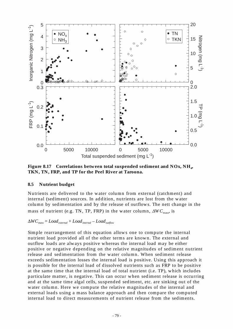
- 79 -

0.0

0.5

1.0

1.5

2.0

0 5000 100000.0

0.1

0.2

0.30

1

2

3

4

5

TNTKN

NOxNH3

Inor

gani

c N

itrog

en (

mg

L-1)

FR

P (

mg

L-1) T

P (m

g L-1)

Nitrogen (m

g L-1)

0

5

10

15

20

0 5000 10000Total suspended sediment (mg L-1)

Figure 8.17 Correlations between total suspended sediment and NOx, NH4,TKN, TN, FRP, and TP for the Peel River at Taroona.

8.5 Nutrient budget

Nutrients are delivered to the water column from external (catchment) andinternal (sediment) sources. In addition, nutrients are lost from the watercolumn by sedimentation and by the release of outflows. The nett change in themass of nutrient (e.g. TN, TP, FRP) in the water column, ∆WCmass, is

∆WCmass = Loadexternal + Loadinternal – Loadoutflow

Simple rearrangement of this equation allows one to compute the internalnutrient load provided all of the other terms are known. The external andoutflow loads are always positive whereas the internal load may be eitherpositive or negative depending on the relative magnitudes of sediment nutrientrelease and sedimentation from the water column. When sediment releaseexceeds sedimentation losses the internal load is positive. Using this approach itis possible for the internal load of dissolved nutrients such as FRP to be positiveat the same time that the internal load of total nutrient (i.e. TP), which includesparticulate matter, is negative. This can occur when sediment release is occurringand at the same time algal cells, suspended sediment, etc. are sinking out of thewater column. Here we compute the relative magnitudes of the internal andexternal loads using a mass balance approach and then compare the computedinternal load to direct measurements of nutrient release from the sediments.

- 80 -

When the inflow and outflow concentrations vary over time, the nett internalload of a nutrient during a time interval, ∆t, can be c o m p u ted as

Loadinternal = C(z)A(z)dz

0‘

H

t

t + ∆t

– QiCi – QoCo dtt

t + ∆t

H e r e Qi, Q o, Ci, Co a r e t h e inflow and outflow discharges and concentrations,respectively, H is the depth of the water column, A(z) is the surface area at heightz, C(z) is the concentration at height z, and t is the time. The first term on theright-hand side is simply ∆WCmass and the second term gives the net delivery orloss of nutrient due to inflows and release. A negative value for the internal loadrepresents a loss of nutrient to the sediments of the reservoir.

The calculations use both historical and contemporary data. Water columnchemical profiles collected at Stn 1 were assumed to be representative of thereservoir as a whole and inflow loads were computed from data collected fromthe Peel River at Taroona, 6.7 km upstream of the reservoir, but downstream ofall major tributaries but one.

The total Peel River nutrient load consists of base flow and ‘event’ flowcomponents. An inflow event is defined to occur whenever the water level at theTaroona gauging station exceeds 0.7 m (= 540 ML d-1), which is the thresholdrequired to trigger the automated sampler. To determine the nutrient load of aninflow event, a curve (typically a cubic spline) was fitted to the concentration datatime series from samples taken throughout the inflow event. The curve was thenused to interpolate in time between measured values to produce a concentrationtime series that matched the 15-minute resolution of the flow data. Finally, theproduct of the concentration and the flow rate was integrated over time for theduration of the inflow event to calculate the total mass of nutrient associatedwith the event.

Estimates of the amount of phosphorus and nitrogen exported downstream ofthe reservoir were made by muliplying the volume of water released by theaverage concentrations of TN, TP, and FRP in the water column at the depth ofthe outlet (Figure 4.4).

The basis for each mass balance has been defined as the period just after winteroverturn until the first complete mixing event the next year. This methodprovides a realistic description of the annual cycling of nutrients and a moreaccurate basis for comparison of the nutrient status of the water body from year toyear. The amount of nutrient present in dissolved form in the water columnduring summer is highly variable due to the unpredictability of the onset, andmagnitude, of permanent stratification in years when the destratifier has beenoperated. By contrast, the annual winter overturn is relatively consistent and thesystem, in terms of the nutrient dynamics, is essentially returned to itsequilibrium state or initial condition at this time.

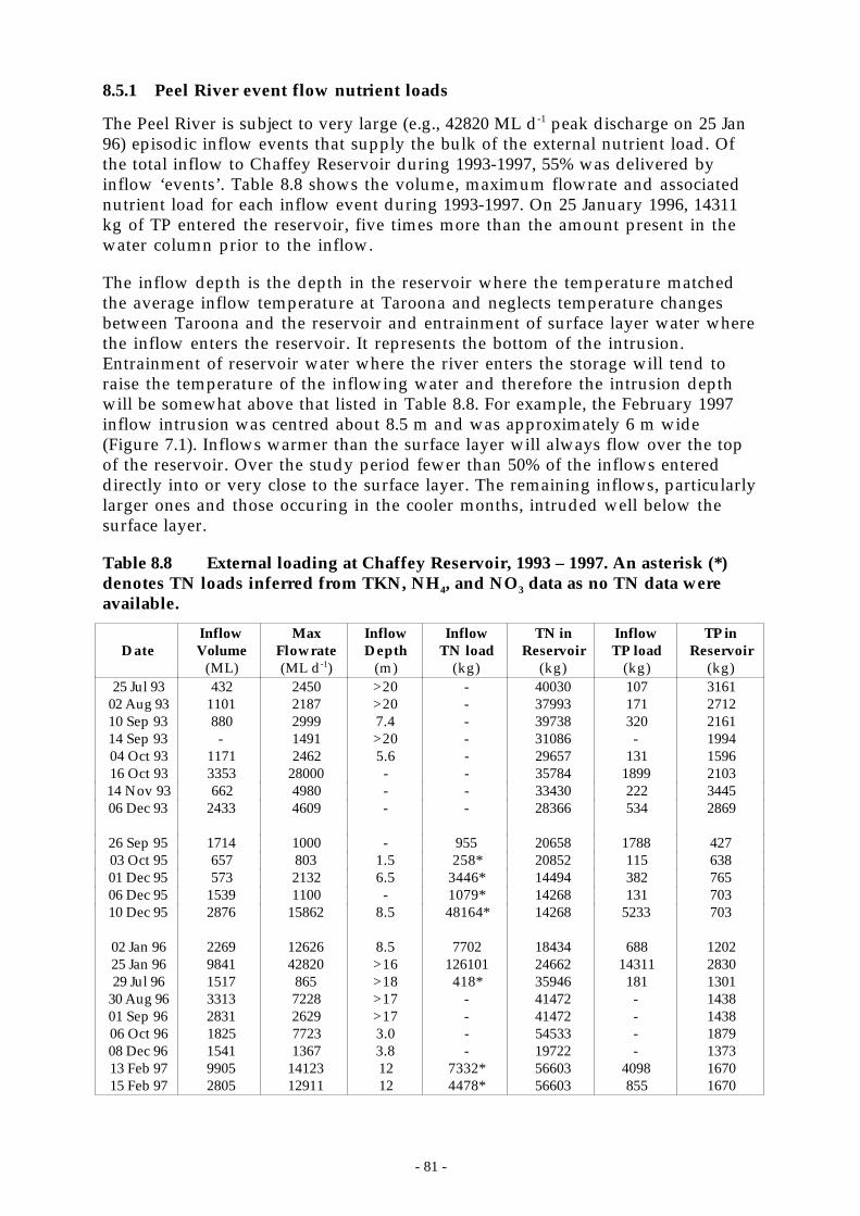
- 81 -

8.5.1 Peel River event flow nutrient loads

The Peel River is subject to very large (e.g., 42820 ML d-1 peak discharge on 25 Jan96) episodic inflow events that supply the bulk of the external nutrient load. Ofthe total inflow to Chaffey Reservoir during 1993-1997, 55% was delivered byinflow ‘events’. Table 8.8 shows the volume, maximum flowrate and associatednutrient load for each inflow event during 1993-1997. On 25 January 1996, 14311kg of TP entered the reservoir, five times more than the amount present in thewater column prior to the inflow.

The inflow depth is the depth in the reservoir where the temperature matchedthe average inflow temperature at Taroona and neglects temperature changesbetween Taroona and the reservoir and entrainment of surface layer water wherethe inflow enters the reservoir. It represents the bottom of the intrusion.Entrainment of reservoir water where the river enters the storage will tend toraise the temperature of the inflowing water and therefore the intrusion depthwill be somewhat above that listed in Table 8.8. For example, the February 1997inflow intrusion was centred about 8.5 m and was approximately 6 m wide(Figure 7.1). Inflows warmer than the surface layer will always flow over the topof the reservoir. Over the study period fewer than 50% of the inflows entereddirectly into or very close to the surface layer. The remaining inflows, particularlylarger ones and those occuring in the cooler months, intruded well below thesurface layer.

Table 8.8 External loading at Chaffey Reservoir, 1993 – 1997. An asterisk (*)denotes TN loads inferred from TKN, NH4, and NO3 data as no TN data wereavailable.

DateInflowVolume

(ML)

MaxFlowrate(ML d-1)

InflowDepth

(m)

InflowTN load

(kg)

TN inReservoir

(kg)

InflowTP load

(kg)

TP inReservoir

(kg)25 Jul 93 432 2450 >20 - 40030 107 3161

02 Aug 93 1101 2187 >20 - 37993 171 271210 Sep 93 880 2999 7.4 - 39738 320 216114 Sep 93 - 1491 >20 - 31086 - 199404 Oct 93 1171 2462 5.6 - 29657 131 159616 Oct 93 3353 28000 - - 35784 1899 210314 Nov 93 662 4980 - - 33430 222 344506 Dec 93 2433 4609 - - 28366 534 2869

26 Sep 95 1714 1000 - 955 20658 1788 42703 Oct 95 657 803 1.5 258* 20852 115 63801 Dec 95 573 2132 6.5 3446* 14494 382 76506 Dec 95 1539 1100 - 1079* 14268 131 70310 Dec 95 2876 15862 8.5 48164* 14268 5233 703

02 Jan 96 2269 12626 8.5 7702 18434 688 120225 Jan 96 9841 42820 >16 126101 24662 14311 283029 Jul 96 1517 865 >18 418* 35946 181 1301

30 Aug 96 3313 7228 >17 - 41472 - 143801 Sep 96 2831 2629 >17 - 41472 - 143806 Oct 96 1825 7723 3.0 - 54533 - 187908 Dec 96 1541 1367 3.8 - 19722 - 137313 Feb 97 9905 14123 12 7332* 56603 4098 167015 Feb 97 2805 12911 12 4478* 56603 855 1670

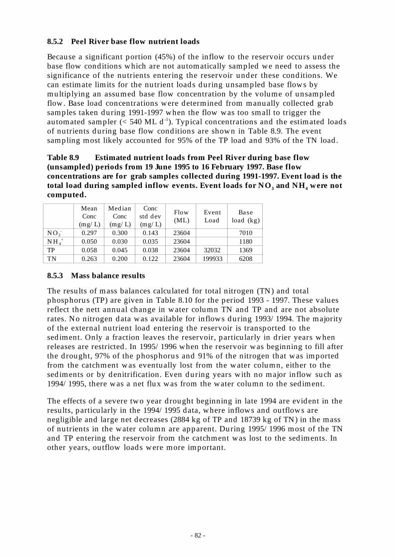
- 82 -

8.5.2 Peel River base flow nutrient loads

Because a significant portion (45%) of the inflow to the reservoir occurs underbase flow conditions which are not automatically sampled we need to assess thesignificance of the nutrients entering the reservoir under these conditions. Wecan estimate limits for the nutrient loads during unsampled base flows bymultiplying an assumed base flow concentration by the volume of unsampledflow. Base load concentrations were determined from manually collected grabsamples taken during 1991-1997 when the flow was too small to trigger theautomated sampler (< 540 ML d-1). Typical concentrations and the estimated loadsof nutrients during base flow conditions are shown in Table 8.9. The eventsampling most likely accounted for 95% of the TP load and 93% of the TN load.

Table 8.9 Estimated nutrient loads from Peel River during base flow(unsampled) periods from 19 June 1995 to 16 February 1997. Base flowconcentrations are for grab samples collected during 1991-1997. Event load is thetotal load during sampled inflow events. Event loads for NO3 and NH4 were notcomputed.

MeanConc

(mg/L)

MedianConc

(mg/L)

Concstd dev(mg/L)

Flow(ML)

EventLoad

Baseload (kg)

NO3- 0.297 0.300 0.143 23604 7010

NH4+ 0.050 0.030 0.035 23604 1180

TP 0.058 0.045 0.038 23604 32032 1369TN 0.263 0.200 0.122 23604 199933 6208

8.5.3 Mass balance results

The results of mass balances calculated for total nitrogen (TN) and totalphosphorus (TP) are given in Table 8.10 for the period 1993 - 1997. These valuesreflect the nett annual change in water column TN and TP and are not absoluterates. No nitrogen data was available for inflows during 1993/1994. The majorityof the external nutrient load entering the reservoir is transported to thesediment. Only a fraction leaves the reservoir, particularly in drier years whenreleases are restricted. In 1995/1996 when the reservoir was beginning to fill afterthe drought, 97% of the phosphorus and 91% of the nitrogen that was importedfrom the catchment was eventually lost from the water column, either to thesediments or by denitrification. Even during years with no major inflow such as1994/1995, there was a net flux was from the water column to the sediment.

The effects of a severe two year drought beginning in late 1994 are evident in theresults, particularly in the 1994/1995 data, where inflows and outflows arenegligible and large net decreases (2884 kg of TP and 18739 kg of TN) in the massof nutrients in the water column are apparent. During 1995/1996 most of the TNand TP entering the reservoir from the catchment was lost to the sediments. Inother years, outflow loads were more important.

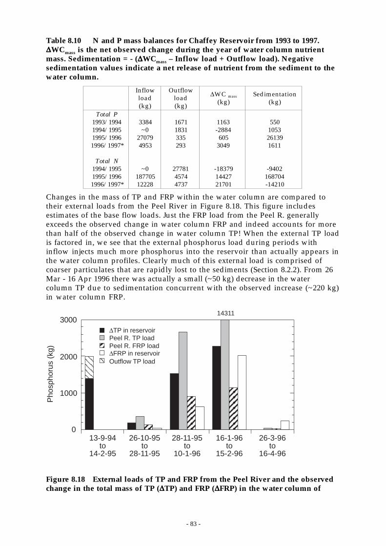
- 83 -

Table 8.10 N and P mass balances for Chaffey Reservoir from 1993 to 1997.∆∆∆∆WCmass is the net observed change during the year of water column nutrientmass. Sedimentation = - (∆∆∆∆WCmass – Inflow load + Outflow load). Negativesedimentation values indicate a net release of nutrient from the sediment to thewater column.

Inflowload(kg)

Outflowload(kg)

∆WC mass

(kg)Sedimentation

(kg)

Total P1993/1994 3384 1671 1163 5501994/1995 ~0 1831 -2884 10531995/1996 27079 335 605 261391996/1997* 4953 293 3049 1611

Total N1994/1995 ~0 27781 -18379 -94021995/1996 187705 4574 14427 1687041996/1997* 12228 4737 21701 -14210

Changes in the mass of TP and FRP within the water column are compared totheir external loads from the Peel River in Figure 8.18. This figure includesestimates of the base flow loads. Just the FRP load from the Peel R. generallyexceeds the observed change in water column FRP and indeed accounts for morethan half of the observed change in water column TP! When the external TP loadis factored in, we see that the external phosphorus load during periods withinflow injects much more phosphorus into the reservoir than actually appears inthe water column profiles. Clearly much of this external load is comprised ofcoarser particulates that are rapidly lost to the sediments (Section 8.2.2). From 26Mar - 16 Apr 1996 there was actually a small (~50 kg) decrease in the watercolumn TP due to sedimentation concurrent with the observed increase (~220 kg)in water column FRP.

0

1000

2000

300014311

13-9-94to

14-2-95

26-10-95to

28-11-95

28-11-95to

10-1-96

16-1-96to

15-2-96

26-3-96to

16-4-96

Pho

spho

rus

(kg)

Outflow TP load

∆TP in reservoirPeel R. TP loadPeel R. FRP load∆FRP in reservoir

Figure 8.18 External loads of TP and FRP from the Peel River and the observedchange in the total mass of TP (∆∆∆∆TP) and FRP (∆∆∆∆FRP) in the water column of

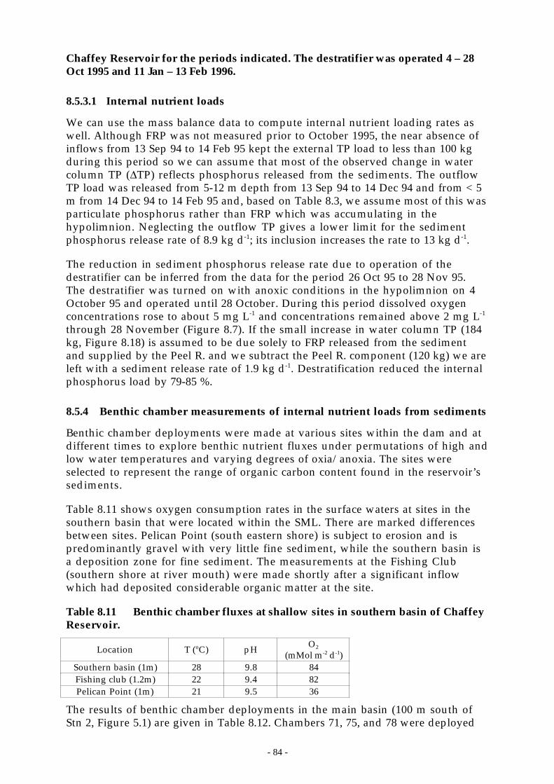
- 84 -

Chaffey Reservoir for the periods indicated. The destratifier was operated 4 – 28Oct 1995 and 11 Jan – 13 Feb 1996.

8.5.3.1 Internal nutrient loads

We can use the mass balance data to compute internal nutrient loading rates aswell. Although FRP was not measured prior to October 1995, the near absence ofinflows from 13 Sep 94 to 14 Feb 95 kept the external TP load to less than 100 kgduring this period so we can assume that most of the observed change in watercolumn TP (∆TP) reflects phosphorus released from the sediments. The outflowTP load was released from 5-12 m depth from 13 Sep 94 to 14 Dec 94 and from < 5m from 14 Dec 94 to 14 Feb 95 and, based on Table 8.3, we assume most of this wasparticulate phosphorus rather than FRP which was accumulating in thehypolimnion. Neglecting the outflow TP gives a lower limit for the sedimentphosphorus release rate of 8.9 kg d-1; its inclusion increases the rate to 13 kg d-1.

The reduction in sediment phosphorus release rate due to operation of thedestratifier can be inferred from the data for the period 26 Oct 95 to 28 Nov 95.The destratifier was turned on with anoxic conditions in the hypolimnion on 4October 95 and operated until 28 October. During this period dissolved oxygenconcentrations rose to about 5 mg L-1 and concentrations remained above 2 mg L-1

through 28 November (Figure 8.7). If the small increase in water column TP (184kg, Figure 8.18) is assumed to be due solely to FRP released from the sedimentand supplied by the Peel R. and we subtract the Peel R. component (120 kg) we areleft with a sediment release rate of 1.9 kg d-1. Destratification reduced the internalphosphorus load by 79-85 %.

8.5.4 Benthic chamber measurements of internal nutrient loads from sediments

Benthic chamber deployments were made at various sites within the dam and atdifferent times to explore benthic nutrient fluxes under permutations of high andlow water temperatures and varying degrees of oxia/anoxia. The sites wereselected to represent the range of organic carbon content found in the reservoir’ssediments.

Table 8.11 shows oxygen consumption rates in the surface waters at sites in thesouthern basin that were located within the SML. There are marked differencesbetween sites. Pelican Point (south eastern shore) is subject to erosion and ispredominantly gravel with very little fine sediment, while the southern basin isa deposition zone for fine sediment. The measurements at the Fishing Club(southern shore at river mouth) were made shortly after a significant inflowwhich had deposited considerable organic matter at the site.

Table 8.11 Benthic chamber fluxes at shallow sites in southern basin of ChaffeyReservoir.

Location T (oC) pH O2

(mMol m-2 d-1)Southern basin (1m) 28 9.8 84Fishing club (1.2m) 22 9.4 82Pelican Point (1m) 21 9.5 36

The results of benthic chamber deployments in the main basin (100 m south ofStn 2, Figure 5.1) are given in Table 8.12. Chambers 71, 75, and 78 were deployed

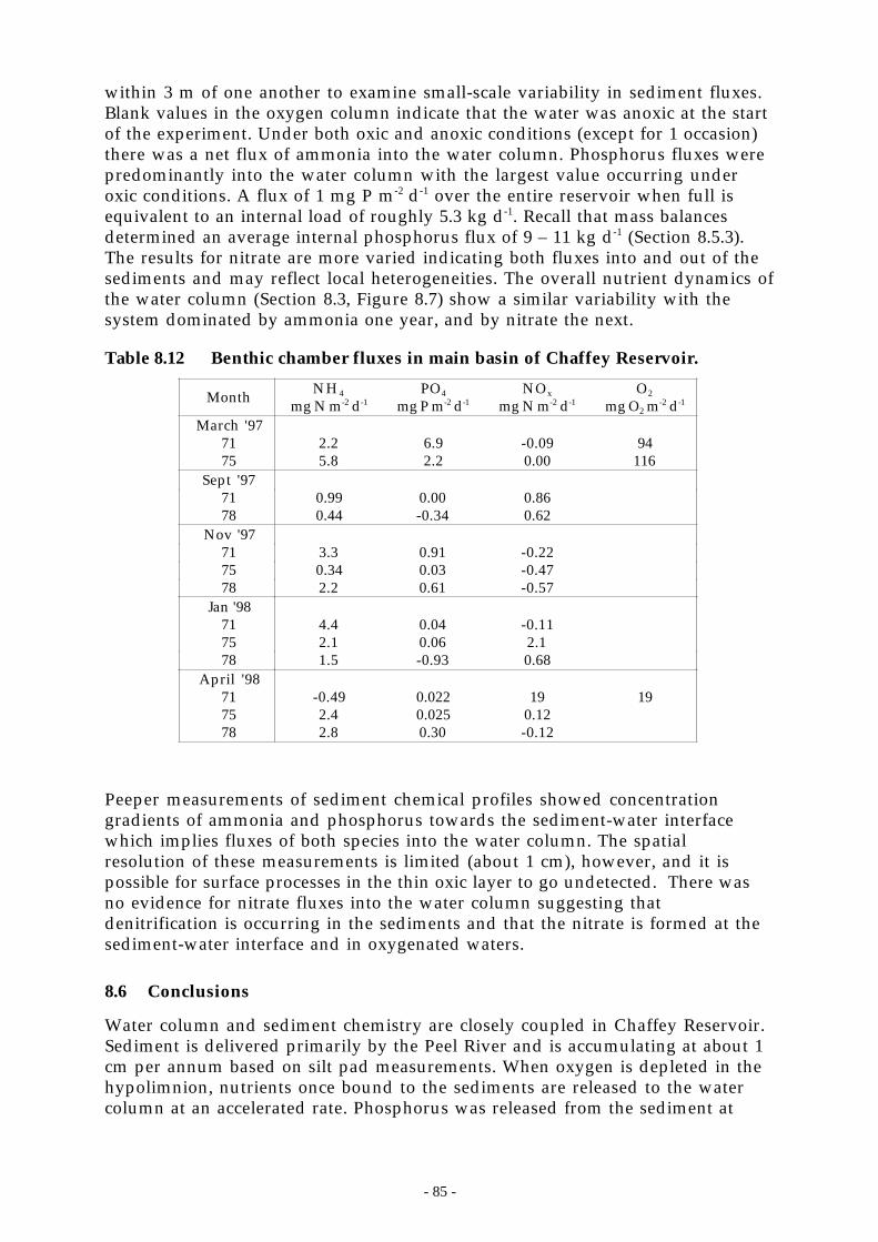
- 85 -

within 3 m of one another to examine small-scale variability in sediment fluxes.Blank values in the oxygen column indicate that the water was anoxic at the startof the experiment. Under both oxic and anoxic conditions (except for 1 occasion)there was a net flux of ammonia into the water column. Phosphorus fluxes werepredominantly into the water column with the largest value occurring underoxic conditions. A flux of 1 mg P m-2 d-1 over the entire reservoir when full isequivalent to an internal load of roughly 5.3 kg d-1. Recall that mass balancesdetermined an average internal phosphorus flux of 9 – 11 kg d-1 (Section 8.5.3).The results for nitrate are more varied indicating both fluxes into and out of thesediments and may reflect local heterogeneities. The overall nutrient dynamics ofthe water column (Section 8.3, Figure 8.7) show a similar variability with thesystem dominated by ammonia one year, and by nitrate the next.

Table 8.12 Benthic chamber fluxes in main basin of Chaffey Reservoir.

Month NH4

mg N m-2 d-1PO4

mg P m-2 d-1NOx

mg N m-2 d-1O2

mg O2 m-2 d-1

March '9771 2.2 6.9 -0.09 9475 5.8 2.2 0.00 116

Sept '9771 0.99 0.00 0.8678 0.44 -0.34 0.62

Nov '9771 3.3 0.91 -0.2275 0.34 0.03 -0.4778 2.2 0.61 -0.57

Jan '9871 4.4 0.04 -0.1175 2.1 0.06 2.178 1.5 -0.93 0.68

April '9871 -0.49 0.022 19 1975 2.4 0.025 0.1278 2.8 0.30 -0.12

Peeper measurements of sediment chemical profiles showed concentrationgradients of ammonia and phosphorus towards the sediment-water interfacewhich implies fluxes of both species into the water column. The spatialresolution of these measurements is limited (about 1 cm), however, and it ispossible for surface processes in the thin oxic layer to go undetected. There wasno evidence for nitrate fluxes into the water column suggesting thatdenitrification is occurring in the sediments and that the nitrate is formed at thesediment-water interface and in oxygenated waters.

8.6 Conclusions

Water column and sediment chemistry are closely coupled in Chaffey Reservoir.Sediment is delivered primarily by the Peel River and is accumulating at about 1cm per annum based on silt pad measurements. When oxygen is depleted in thehypolimnion, nutrients once bound to the sediments are released to the watercolumn at an accelerated rate. Phosphorus was released from the sediment at

- 86 -

roughly 10 kg d-1(~ 4.5-5 mg P m-2 d-1) and was mostly orthophosphate. Operationof the destratifier reduced the internal phosphorus load by 80%.

When the water column is anoxic, iron and manganese are presentpredominantly in colloidal form as FeS and MnS. Neither species has a highcapacity for binding phosphate. These colloids slowly settle out of the watercolumn resulting in a loss of Fe and Mn to the sediments.

Operation of the destratifier oxidises the bottom waters and Fe formerly presentas FeS is converted to FeOOH which subsequently scavenges phosphate. Thescavenging of phosphate is relatively rapid but incomplete (63%) with most of theremoval due to the oxidised Fe species. Manganese oxides appear to be relativelyineffectual in adsorbing P. There is insufficient Fe2+ to provide sufficient ironoxide to completely scavenge all the available P in the anoxic bottom waters ofthe dam. Consequently, operation of the destratification system once anoxia hasbeen established can raise – and not lower – concentrations of bioavailable (ortho-) phosphate at the surface.

The effectiveness of the destratification system in controlling surfaceconcentrations of P would be enhanced by the provision of additional Fe3+ to thesurface layers or by reduction of SO4 so that Fe is not removed in thehypolimnion as FeS.

Destratification increases the temperature of the hypolimnion which in turnincreases O2 demand. Sediment P release may subsequently increase if anoxicconditions are reestablished.

- 87 -

9 Trophic dynamics - algal species succession

The growth of phytoplankton requires light for photosynthesis and nutrients forthe manufacture of cell constituents. The biomass supporting capacity of a waterbody is likely to be the lower of the ‘ceilings’ imposed by the availability of theseresources (Reynolds 1997). It is important to distinguish between the cellreplication rate and the net rate of growth of the algal population; cell replicationcan occur at near maximal rates even if biomass is not accumulating providednutrients are recycled quickly within the euphotic zone. The cell replication ratedepends most strongly on light availability and temperature as the time scaleassociated with nutrient uptake is much shorter than that for photosyntheticfixation of CO2 (Reynolds and Irish 1997). Phytoplankton biomass also depends onloss factors such as death, grazing by zooplankton, sedimentation and hydraulicwashout as well as on the overall availability of nutrients.

Nutrient availability can vary temporally and spatially in the water column withstrong vertical gradients in N and P forming during periods of thermalstratification (Section 8.3). Biological consumption can lead to very low inorganicnutrient concentrations in the SML at the same time as inorganic nutrients areaccumulating in the hypolimnion as the result of sediment diagenesis. Re-supplyof nutrients to the SML often requires deepening of the layer to entrain relativelynutrient-rich water from below (Section 7.1, Figure 7.1).

The amount of light available for photosynthesis depends on the attenuation oflight in the water column, the depth of the SML and the amount of turbulence inthe surface layer, q*. In a weakly mixed environment (low q*), migratory orbuoyant phytoplankton can alter their position in the water column to optimiselight availability. As q* increases and the SML deepens, the mean light intensityis reduced providing an advantage to phytoplankton adapted to low-lightconditions. Increasing q* also reduces the rate at which sinking phytoplanktonsuch as diatoms are lost from the surface layer.

In this section we analyse the 11 year record of chemical, physical and algalabundance data and describe the annual and interannual trends in biomass andcommunity succession. We also consider the long term affects of destratification.In addition, we present the results of an intensive study of the algal andzooplankton communities between 1995 and 1997 that included measuring thelight and nutrient requirements of the major algal taxa at Chaffey Dam and theiradaptations to acquisition of these resources.

9.1 Methodology

Water samples were collected between 1987 and 1997 at a number of sites aroundthe reservoir and enumerated to genera by DLWC staff at the ArncliffeLaboratories. Sampling was undertaken at least monthly, but for most of theperiod weekly data were available. The samples were collected using an elbowgrab from about 0.25 m depth; therefore, the samples only representphytoplankton from the surface of the reservoir. Cell abundance for each taxa hasbeen converted to algal volume using mean cell dimensions and the appropriateshape formula. Cell dimensions were measured at MDFRC for the common taxabetween 1995 and 1997 and previous years were assumed to be equivalent.Dimensions for the less common taxa were taken as the mean of the range for

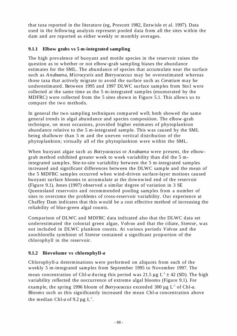
- 88 -

that taxa reported in the literature (eg, Prescott 1982, Entwisle et al. 1997). Dataused in the following analysis represent pooled data from all the sites within thedam and are reported as either weekly or monthly averages.

9.1.1 Elbow grabs vs 5 m-integrated sampling

The high prevalence of buoyant and motile species in the reservoir raises thequestion as to whether or not elbow-grab sampling biases the abundanceestimates for the SML. The abundance of species that accumulate near the surfacesuch as Anabaena, Microcystis and Botryococcus may be overestimated whereasthose taxa that actively migrate to avoid the surface such as Ceratium may beunderestimated. Between 1995 and 1997 DLWC surface samples from Stn1 werecollected at the same time as the 5 m-integrated samples (enumerated by theMDFRC) were collected from the 5 sites shown in Figure 5.1. This allows us tocompare the two methods.

In general the two sampling techniques compared well; both showed the samegeneral trends in algal abundance and species composition. The elbow-grabtechnique, on most occasions, provided higher estimates of phytoplanktonabundance relative to the 5 m-integrated sample. This was caused by the SMLbeing shallower than 5 m and the uneven vertical distribution of thephytoplankton; virtually all of the phytoplankton were within the SML.

When buoyant algae such as Botryococcus or Anabaena were present, the elbow-grab method exhibited greater week to week variability than did the 5 m-integrated samples. Site-to-site variability between the 5 m-integrated samplesincreased and significant differences between the DLWC sample and the mean ofthe 5 MDFRC samples occurred when wind-driven surface-layer motions causedbuoyant surface blooms to accumulate at the downwind end of the reservoir(Figure 9.1). Jones (1997) observed a similar degree of variation in 3 SEQueensland reservoirs and recommended pooling samples from a number ofsites to overcome the problems of cross-reservoir variability. Our experience atChaffey Dam indicates that this would be a cost effective method of increasing thereliability of blue-green algal counts.

Comparison of DLWC and MDFRC data indicated also that the DLWC data setunderestimated the colonial green algae, Volvox and that the ciliate, Stentor, wasnot included in DLWC plankton counts. At various periods Volvox and thezoochlorella symbiont of Stentor contained a significant proportion of thechlorophyll in the reservoir.

9.1.2 Biovolume vs chlorophyll-a

Chlorophyll-a determinations were performed on aliquots from each of theweekly 5 m-integrated samples from September 1995 to November 1997. Themean concentration of Chl-a during this period was 21.5 µg L-1 ± 42 (SD). The highvariability reflected the ooccurrence of extreme algal blooms (Figure 9.1). Forexample, the spring 1996 bloom of Botryococcus exceeded 300 µg L-1 of Chl-a.Blooms such as this significantly increased the mean Chl-a concentration abovethe median Chl-a of 9.2 µg L-1.

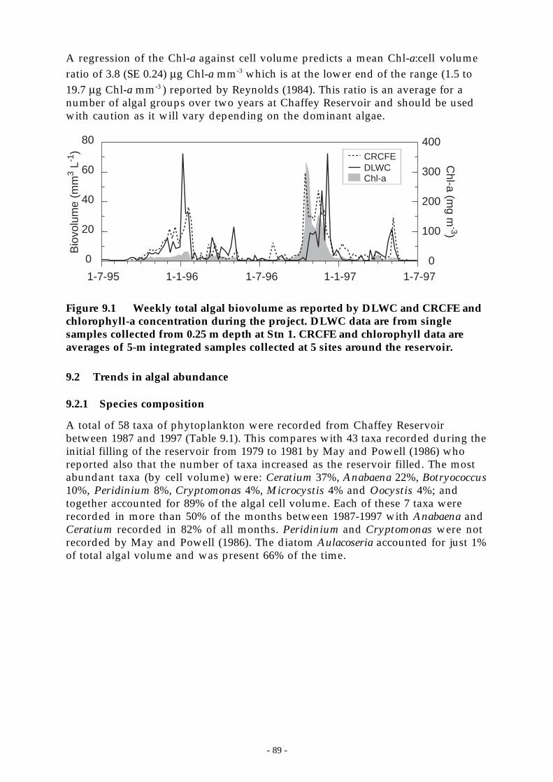
- 89 -

A regression of the Chl-a against cell volume predicts a mean Chl-a:cell volumeratio of 3.8 (SE 0.24) µg Chl-a mm-3 which is at the lower end of the range (1.5 to19.7 µg Chl-a mm-3 ) reported by Reynolds (1984). This ratio is an average for anumber of algal groups over two years at Chaffey Reservoir and should be usedwith caution as it will vary depending on the dominant algae.

Bio

volu

me

(mm

3 L-1

)

0

20

40

60

80

0

100

200

300

400

1-7-95 1-1-96 1-7-96 1-1-97 1-7-97

Chl-a (m

g m-3)

Chl-a

CRCFEDLWC

Figure 9.1 Weekly total algal biovolume as reported by DLWC and CRCFE andchlorophyll-a concentration during the project. DLWC data are from singlesamples collected from 0.25 m depth at Stn 1. CRCFE and chlorophyll data areaverages of 5-m integrated samples collected at 5 sites around the reservoir.

9.2 Trends in algal abundance

9.2.1 Species composition

A total of 58 taxa of phytoplankton were recorded from Chaffey Reservoirbetween 1987 and 1997 (Table 9.1). This compares with 43 taxa recorded during theinitial filling of the reservoir from 1979 to 1981 by May and Powell (1986) whoreported also that the number of taxa increased as the reservoir filled. The mostabundant taxa (by cell volume) were: Ceratium 37%, Anabaena 22%, Botryococcus10%, Peridinium 8%, Cryptomonas 4%, Microcystis 4% and Oocystis 4%; andtogether accounted for 89% of the algal cell volume. Each of these 7 taxa wererecorded in more than 50% of the months between 1987-1997 with Anabaena andCeratium recorded in 82% of all months. Peridinium and Cryptomonas were notrecorded by May and Powell (1986). The diatom Aulacoseria accounted for just 1%of total algal volume and was present 66% of the time.

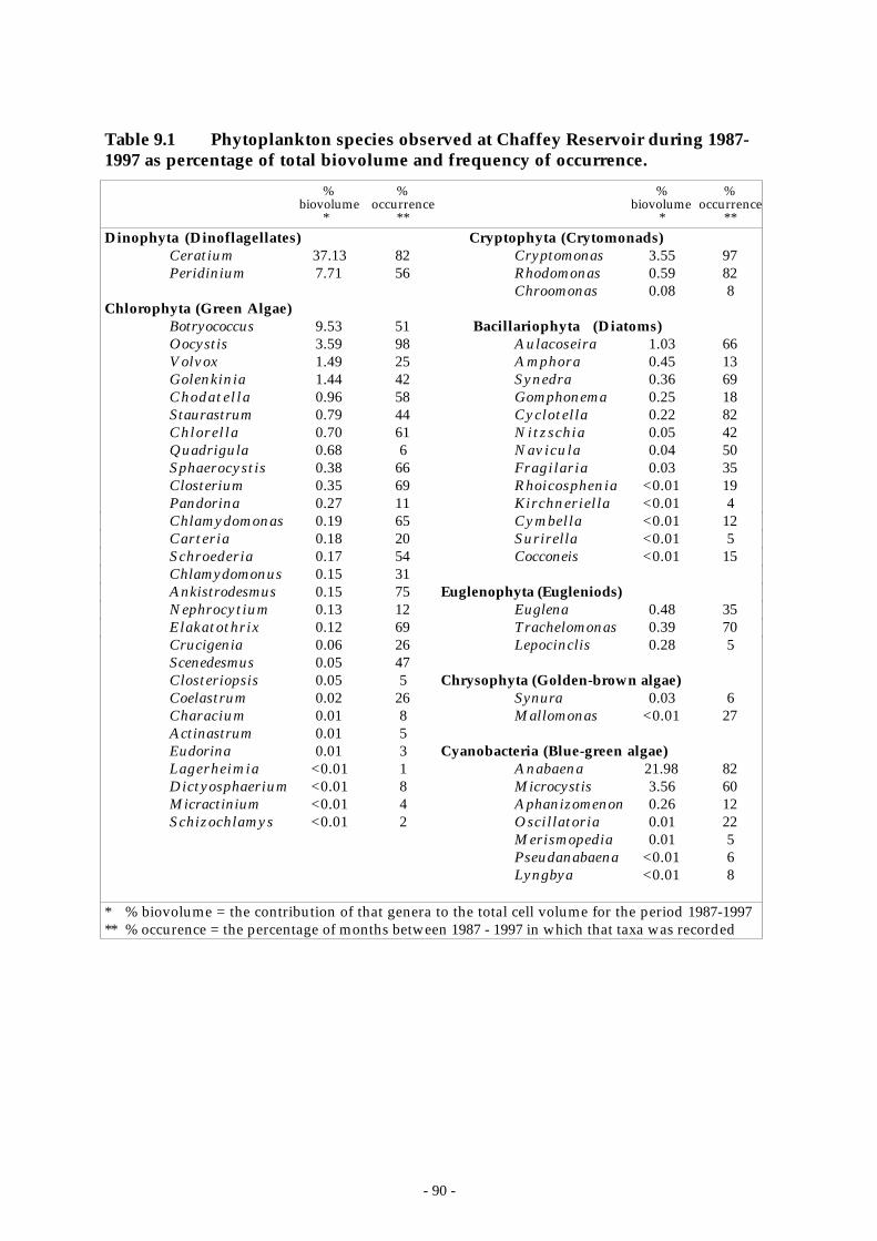
- 90 -

Table 9.1 Phytoplankton species observed at Chaffey Reservoir during 1987-1997 as percentage of total biovolume and frequency of occurrence.

%biovolume

*

%occurrence

**

%biovolume

*

%occurrence

**

Dinophyta (Dinoflagellates) Cryptophyta (Crytomonads)Ceratium 37.13 82 Cryptomonas 3.55 97Peridinium 7.71 56 Rhodomonas 0.59 82

Chroomonas 0.08 8Chlorophyta (Green Algae)

Botryococcus 9.53 51 Bacillariophyta (Diatoms)Oocystis 3.59 98 Aulacoseira 1.03 66Volvox 1.49 25 Amphora 0.45 13Golenkinia 1.44 42 Synedra 0.36 69Choda t e l l a 0.96 58 Gomphonema 0.25 18Staurastrum 0.79 44 Cyclotel la 0.22 82Chlore l l a 0.70 61 Nitzschia 0.05 42Quadrigula 0.68 6 Navicula 0.04 50Sphaerocystis 0.38 66 Fragi lar ia 0.03 35Closterium 0.35 69 Rhoicosphenia <0.01 19Pandorina 0.27 11 Kirchneriel la <0.01 4Chlamydomonas 0.19 65 Cymbel la <0.01 12Carteria 0.18 20 Surirella <0.01 5Schroederia 0.17 54 Cocconeis <0.01 15Chlamydomonus 0.15 31Ankistrodesmus 0.15 75 Euglenophyta (Eugleniods)Nephrocytium 0.13 12 Euglena 0.48 35Elakatothrix 0.12 69 Trachelomonas 0.39 70Crucigenia 0.06 26 Lepocinclis 0.28 5Scenedesmus 0.05 47Closteriopsis 0.05 5 Chrysophyta (Golden-brown algae)Coelastrum 0.02 26 Synura 0.03 6Characium 0.01 8 Mallomonas <0.01 27Actinastrum 0.01 5Eudorina 0.01 3 Cyanobacteria (Blue-green algae)Lagerhe imia <0.01 1 Anabaena 21.98 82Dictyosphaerium <0.01 8 Microcystis 3.56 60Micractinium <0.01 4 Aphanizomenon 0.26 12Schizochlamys <0.01 2 Oscillatoria 0.01 22

Merismopedia 0.01 5Pseudanabaena <0.01 6Lyngbya <0.01 8

* % biovolume = the contribution of that genera to the total cell volume for the period 1987-1997** % occurence = the percentage of months between 1987 - 1997 in which that taxa was recorded

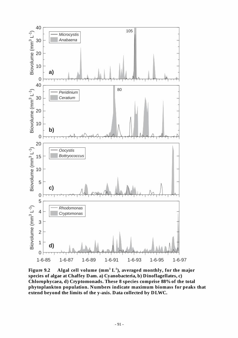
- 91 -

0

1

2

3

4

5

1-6-85 1-6-87 1-6-89 1-6-91 1-6-93 1-6-95 1-6-97

0

10

20

30

400

10

20

30

40

CryptomonasRhodomonas

AnabaenaMicrocystis

CeratiumPeridinium

0

5

10

15

20

BottryococcusOocystis

Bio

volu

me

(mm

3 L-1

)B

iovo

lum

e (m

m3 L

-1)

Bio

volu

me

(mm

3 L-1

)B

iovo

lum

e (m

m3 L

-1)

a)

b)

c)

d)

105

80

Figure 9.2 Algal cell volume (mm3 L-1), averaged monthly, for the majorspecies of algae at Chaffey Dam. a) Cyanobacteria, b) Dinoflagellates, c)Chlorophycaea, d) Cryptomonads. These 8 species comprise 88% of the totalphytoplankton population. Numbers indicate maximum biomass for peaks thatextend beyond the limits of the y-axis. Data collected by DLWC.

- 92 -

9.2.2 Interannual biovolume variability

During 1987-1997 total algal cell volume underwent periods of high and lowabundance with transitions between the two occurring on time scales of weeks toyears (Figure 9.2). There were no distinct seasonal trends; total algal abundanceranged from very low to high in each month of the year. The years with thehighest algal abundance generally had high algal abundance throughout the year,but in particular they had large, persistent blue-green algal and/or dinoflagellateblooms during the winter months. In contrast, years with low algal abundancedid not have blue-green algal or dinoflagellate blooms during the winter months.Algal abundance did not correlate with changes in dam capacity (Figure 6.4),unlike North Pine Dam in SE Queensland (Harris and Baxter, 1996).

The average annual algal volume was calculated for the period betweenturnover4 of the water column in one year with the corresponding period in thefollowing year. It includes contributions from mid-winter, spring and summerblooms and ranged from 3.5 mm3 L-1 in 1987-88, a period of almost continualoperation of the destratifier, to 28.5 mm3 L-1 in 1993-94.

The three largest blooms occurred during the winters of 1991, 1993, and 1994; withlarge populations of Ceratium, which dominated in 1991 and 1994, whileAnabaena and Microcystis dominated in 1993. The large winter blooms of algalspecies that thrive in stratified conditions is consistent with the observation thatthe daily and maximum SML depths can be quite shallow even in winter (Figure7.3) provided an adequate supply of nutrients was available. Large blooms ofCeratium, Anabaena, and Botryococcus also occurred in spring, summer andautumn.

Of the 11 years of algal abundance data, just 2 years (1991-1992 and 1993-1994)contributed 46% of the total algal volume. These two years witnessed the largestwinter blooms since the dam filled and in both cases there were significantinflows to the reservoir prior to the development of the blooms (Figure 6.3). Thevery high winter biomasses may reflect high external nutrient loads at thesetimes. Similarly, the large summer bloom of Ceratium in January 1996 followedsignificant external nutrient loading in the Peel R. during the previous month(Figure 8.18).

The response of the algal population to external nutrient loading events dependscritically on the level at which the inflow intrudes into the reservoir. This levelis determined by the ambient stratification and local climatic conditions at thetime of the inflow (Section 7.1). The algal population is unlikely to respond in theshort term to inflows that intrude below the euphotic zone.

9.2.3 Seasonal biovolume trends

Although the mean monthly biomass at Chaffey Dam did not show a seasonalpattern, analysis of the mean cell abundance and the rate of biomass increase(calculated for monthly averaged cell counts) for major taxa did show some

4 Turnover is assumed to have occurred on the first day of the calendar year when there was a rapidincrease in hypolimnetic O2 accompanied by a decrease in hypolimnetic P. This process usuallyoccurs between April and June, but can occur earlier in summer if artificial destratification isundertaken.

- 93 -

general intra-annual trends. In the rest of this section the term ‘growth’ refers to anet change in biomass of a species and includes losses such as respiration, grazingand sedimentation. It must not be confused with the specific growth rate whichrefers to the cell replication rate. A positive specific growth rate may apply to adeclining population if the loss rates exceed it.

9.2.3.1 Blue-green algae

Between 1987 and 1997 blue-green algae were observed in all months of the yearat least once (Figure 9.2a). Net positive increase of Anabaena biomass hasoccurred in all months of the year, but most frequently in February, March, May,July and September. The fastest increases occurred during March - May as thesurface layer deepened. Rapid biomass accumulation during autumn oftenresulted in a high cell abundance which sometimes persisted, albeit increasing ata slower rate, through winter. If Anabaena was present during November andDecember it was usually declining in abundance and Anabaena were leastabundant in December, January and February.

Microcystis biomass increased most rapidly during late summer and autumn.With the exception of November, which has 3 years in which biomass increased,the remaining months generally have low Microcystis abundance and negativegrowth rates.

9.2.3.2 Green algae

The growth of the Botryococcus population was positive during October for 6 ofthe 11 years, resulting in blooms during spring and summer in 4 of the 11 years(Figure 9.2c). High cell abundance may persist through autumn. Botryococcusbiomass increased slowly in autumn and winter, especially June when anypersistent blooms generally disappeared.

Oocystis exhibited a clear annual trend in cell abundance with relatively highabundance during late spring and summer and low abundance during wintermonths. Oocystis biomass increased the fastest during October and November.The rate of increase usually declined in December and January. Occasionallybiomass increased during autumn and winter, however, this was relatively slowand did not result in high algal abundance.

The major green algal taxa had their highest net growth rates and maximumbiomass between August and November, coincident with the strengthening ofwater column stability, increasing surface mixed layer temperature and increasingsolar insolation.

9.2.3.3 Dinoflagellates

The biomass of Ceratium could increase in all months of the year, however,mean abundance was much greater during the winter months with the exceptionof one large bloom occurring during December 1995 and January 1996 (Figure9.2b). Peridinium biomass generally increased during February, leading to a highabundance during autumn which declined by winter. There were largeinterannual differences in abundance of the dinoflagellates.

- 94 -

In temperate water bodies the dinoflagellates Peridinium and Ceratium aregenerally observed in high abundance during the later stages of stratification,where their relatively low surface-to volume ratios, large size and poor growthcapacity are offset by the ability to avoid grazing and to self regulate verticalposition in the water column to gain access to light and nutrient (e.g., Reynolds1997). In Chaffey Dam, their ability to flourish year round suggests that mixedlayer turbulence, at least in some years (e.g., 1991 and 1993) is low enoughthrough winter for Ceratium to be advantaged.

9.2.3.4 Cryptomonads

Cryptomonas and Rhodomonas were ubiquitous in the surface water throughoutthe year with Cryptomonas occurring in 97% of the months between 1987-1997(Table 9.1, Figure 9.2d). During periods of low algal abundance, crytomonads maydominate algal cell volume but do not reach a high biomass. The biomass ofcryptomonads may increase in any month of the year, but this was most likelyduring spring as the temperature in the surface layer increased along withincreases in solar insolation.

Cryptomonads are almost ubiquitous in surface waters and are relatively moreabundant in moderately enriched waters. Their motility means they are notsolely dependant on stratification or mixing for access to light and nutrient. Theyare considered to be a favourite food of many zooplankton and are thussusceptible to grazing pressure (Reynolds 1997).

9.2.3.5 Diatoms

Generally, there was very low abundance of diatoms at Chaffey Dam withAulacoseria, at 1% of the total biovolume, being the most abundant (Table 9.1).Aulacoseria biomass is likely to increase in late summer (February to April, 5 of11 years) with another period in August (4 of 11 years).

A large epiphytic diatom population, which included Aulacoseria,Gomphomena, Fragillaria and Cyclotella, developed in association with aCladophera dominated benthic mat during the spring of 1997. This populationwas not planktonic, and so did not appear in the water column samples.

In temperate water bodies diatoms are generally found relatively early in thestratification sequence, relying on water column turbulence to maintain theirposition in the surface mixed layer. At Chaffey Dam, they appear in late summerand autumn as the surface layer begins to deepen and occasionally in August.There is sufficient nutrient, including Si, in Chaffey Dam to support large diatompopulations and diatoms are almost always present in the record, though at verylow abundance. This suggests that diatom abundance is limited by either theavailability of light or, more likely, by high loss rates due to the strong persistentstratification.

9.2.3.6 Is there a generalised annual successional sequence at Chaffey Dam?

No clear successional sequence of phytoplankton was observed at Chaffey Dam,however, there was a periodicity of occurrence. During spring and early summerthe biomass of many of the major taxa increased but it was green algae such as

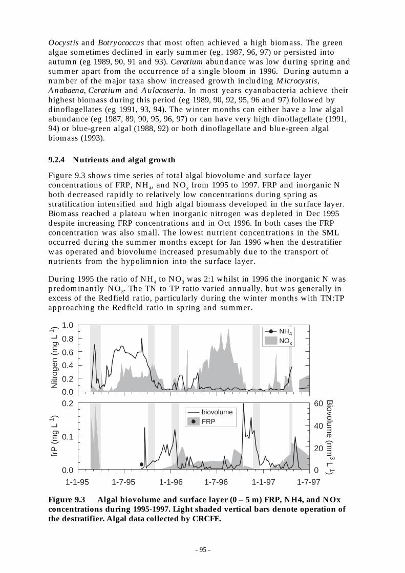
- 95 -

Oocystis and Botryococcus that most often achieved a high biomass. The greenalgae sometimes declined in early summer (eg. 1987, 96, 97) or persisted intoautumn (eg 1989, 90, 91 and 93). Ceratium abundance was low during spring andsummer apart from the occurrence of a single bloom in 1996. During autumn anumber of the major taxa show increased growth including Microcystis,Anabaena, Ceratium and Aulacoseria. In most years cyanobacteria achieve theirhighest biomass during this period (eg 1989, 90, 92, 95, 96 and 97) followed bydinoflagellates (eg 1991, 93, 94). The winter months can either have a low algalabundance (eg 1987, 89, 90, 95, 96, 97) or can have very high dinoflagellate (1991,94) or blue-green algal (1988, 92) or both dinoflagellate and blue-green algalbiomass (1993).

9.2.4 Nutrients and algal growth

Figure 9.3 shows time series of total algal biovolume and surface layerconcentrations of FRP, NH4, and NOx from 1995 to 1997. FRP and inorganic Nboth decreased rapidly to relatively low concentrations during spring asstratification intensified and high algal biomass developed in the surface layer.Biomass reached a plateau when inorganic nitrogen was depleted in Dec 1995despite increasing FRP concentrations and in Oct 1996. In both cases the FRPconcentration was also small. The lowest nutrient concentrations in the SMLoccurred during the summer months except for Jan 1996 when the destratifierwas operated and biovolume increased presumably due to the transport ofnutrients from the hypolimnion into the surface layer.

During 1995 the ratio of NH4 to NO3 was 2:1 whilst in 1996 the inorganic N waspredominantly NO3. The TN to TP ratio varied annually, but was generally inexcess of the Redfield ratio, particularly during the winter months with TN:TPapproaching the Redfield ratio in spring and summer.

Nitr

ogen

(m

g L-1

)

0.0

0.2

0.4

0.6

0.8

1.0

frP

(m

g L-1

)

0.0

0.1

0.2

0

20

40

60

Biovolum

e (mm

3 L-1)

FRPbiovolume

1-1-95 1-7-95 1-1-96 1-7-96 1-1-97 1-7-97

NOx

NH4

Figure 9.3 Algal biovolume and surface layer (0 – 5 m) FRP, NH4, and NOxconcentrations during 1995-1997. Light shaded vertical bars denote operation ofthe destratifier. Algal data collected by CRCFE.

- 96 -

9.2.4.1 Algal growth ‘events’

Prior to the commencement of artificial destratification in late February 1995 thereservoir was strongly stratified with low concentrations of inorganic N (<0.02mgL-1) and FRP (0.004 mgL-1) in the surface layer and very high concentrations ofFRP (0.415 mgL-1) and NH4 (1.1 mgL-1) in the anoxic hypolimnion. Chlorophyllconcentration in the surface layer was 20 _g L-1 and the algal community wascomprised of Oocystis sp. and Cryptomonas sp. with low numbers of Anabaenaand Microcystis. Whilst there was a low concentration of FRP in the surfacewater, algal bioassays and in situ physiological assays (Section 9.2.4.3, Wood andOliver 1995) indicated algal growth to be N-limited. Since, however, Anabaenahas the capacity to fix N2, its biomass would probably be limited by the availabilityof P. Destratification resulted in a rapid increase in the concentration of FRP andNH4 in the mixed layer with FRP concentration in the SML at the end of theperiod of artificial destratification (28 Mar 95) being 0.01 mg L-1. and NH4 rising to0.18 mg L-1 during the period of artificial destratification. During this periodchlorophyll concentration doubled and the algal community became dominatedby Anabaena and Microcystis .

In early January 1996 the SML FRP concentration was < 0.01 mg L-1 and inorganic-N was 0.035 mg L-1. An algal bioassay (10-1-96) indicated that algal biomass,dominated by Ceratium (Figure 9.2b), was limited by the availability of P (Table9.2). Anabaena and Microcystis were not present in the samples collected duringthis time. In late January, heavy grazing by Asplanchna (Section 9.4) reduced theCeratium population, which may have suffered also from poorer lightavailability caused by increased turbidity due to a large inflow from the Peel R.(25-1-96) and a signficant deepening of the SML (10 Feb 96 to 17 Feb 96). Operationof the destratifier (11-1-96 to 15 Feb 96) in addition to the inflow and SMLdeepening increased surface layer FRP to 0.095 mg L-1 and NH4 to 0.23 mg L-1 .Following this large increase in FRP and NH4 Microcystis and Anabaena firstappeared on 6 Feb 96 and 20 Feb 96 respectively, and cell number increased rapidlyuntil late March (Figure 9.4). Notice that the Microcystis responded two weeksearlier than did the Anabaena, presumably due to the pulse of NH4 in earlyFebruary. Anabaena growth appears to have responded to the pulse of NOx inearly March.

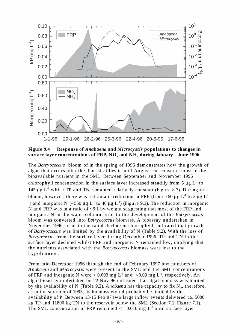
- 97 -

10-4

10-3

10-2

10-1

100

101

0.00

0.02

0.04

0.06

0.08

0.10

0.00

0.20

0.40

0.60

0.80

1-1-96 29-1-96 26-2-96 25-3-96 22-4-96 20-5-96 17-6-96

Biovolum

e (mm

3 L-1)

FRPMicrocystis

NOxNH4

Nitr

ogen

(m

g L-1

)fr

P (

mg

L-1)

Anabaena

Figure 9.4 Response of Anabaena and Microcystis populations to changes insurface layer concentrations of FRP, NOx and NH4 during January – June 1996.

The Botryococcus bloom of in the spring of 1996 demonstrates how the growth ofalgae that occurs after the dam stratifies in mid-August can consume most of thebioavailable nutrient in the SML. Between September and November 1996chlorophyll concentration in the surface layer increased steadily from 5 µg L-1 to145 µg L-1 whilst TP and TN remained relatively constant (Figure 8.7). During thisbloom, however, there was a dramatic reduction in FRP (from ~60 µg L-1 to 3 µg L-

1) and inorganic N (~550 µg L-1 to 40 µg L-1) (Figure 9.3). The reduction in inorganicN and FRP was in a ratio of ~9:1 by weight suggesting that most of the FRP andinorganic N in the water column prior to the development of the Botryococcusbloom was converted into Botryococcus biomass. A bioassay undertaken inNovember 1996, prior to the rapid decline in chlorophyll, indicated that growthof Botryococcus was limited by the availability of N (Table 9.2). With the loss ofBotryococcus from the surface layer during December 1996, TP and TN in thesurface layer declined whilst FRP and inorganic N remained low, implying thatthe nutrients associated with the Botryococcus biomass were lost to thehypolimnion.

From mid-December 1996 through the end of February 1997 low numbers ofAnabaena and Microcystis were present in the SML and the SML concentrationsof FRP and inorganic N were < 0.003 mg L-1 and <0.03 mg L-1, respectively. Analgal bioassay undertaken on 22 Nov 96 indicated that algal biomass was limitedby the availability of N (Table 9.2). Anabaena has the capacity to fix N2, therefore,as in the summer of 1995, its biomass would probably be limited by theavailability of P. Between 13-15 Feb 97 two large inflow events delivered ca. 5000kg TP and 11800 kg TN to the reservoir below the SML (Section 7.1, Figure 7.1).The SML concentration of FRP remained <= 0.010 mg L-1 until surface layer

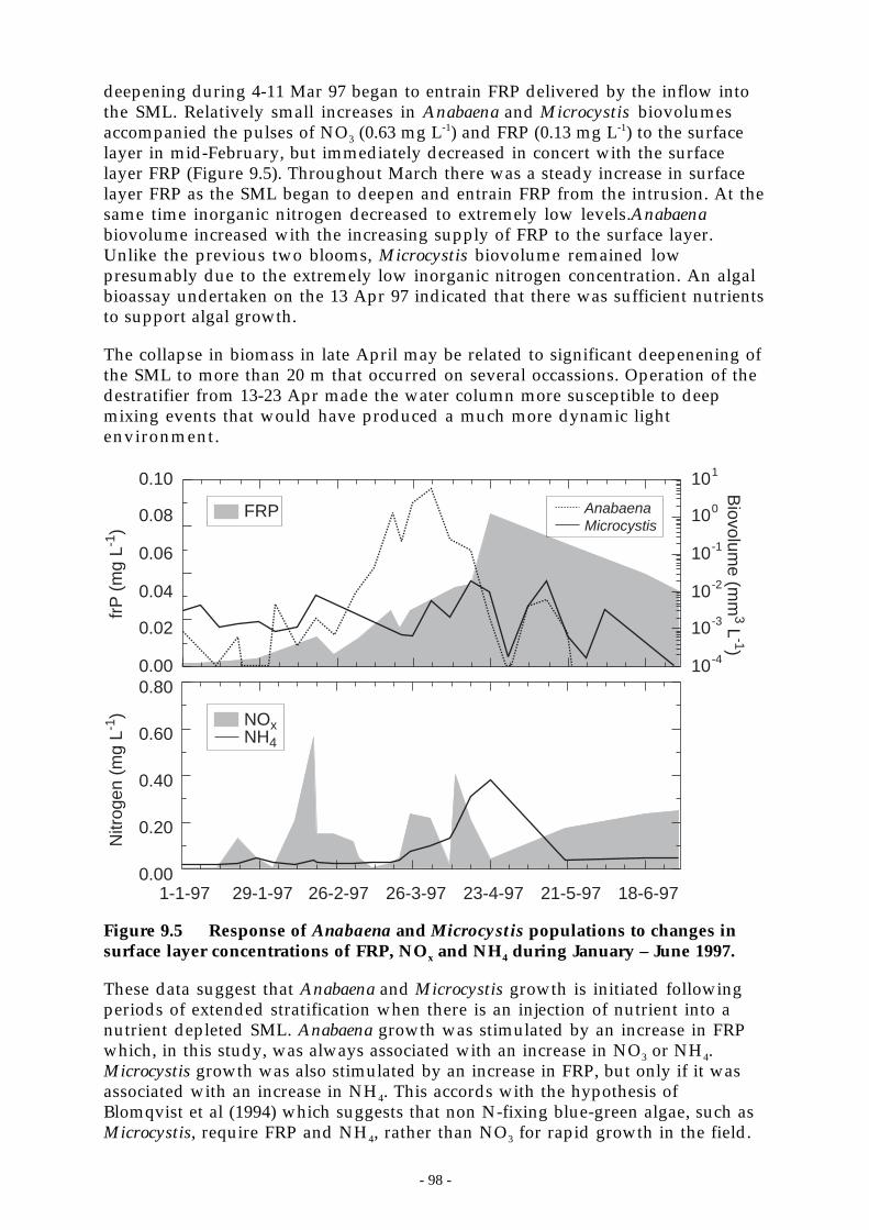
- 98 -

deepening during 4-11 Mar 97 began to entrain FRP delivered by the inflow intothe SML. Relatively small increases in Anabaena and Microcystis biovolumesaccompanied the pulses of NO3 (0.63 mg L-1) and FRP (0.13 mg L-1) to the surfacelayer in mid-February, but immediately decreased in concert with the surfacelayer FRP (Figure 9.5). Throughout March there was a steady increase in surfacelayer FRP as the SML began to deepen and entrain FRP from the intrusion. At thesame time inorganic nitrogen decreased to extremely low levels.Anabaenabiovolume increased with the increasing supply of FRP to the surface layer.Unlike the previous two blooms, Microcystis biovolume remained lowpresumably due to the extremely low inorganic nitrogen concentration. An algalbioassay undertaken on the 13 Apr 97 indicated that there was sufficient nutrientsto support algal growth.

The collapse in biomass in late April may be related to significant deepenening ofthe SML to more than 20 m that occurred on several occassions. Operation of thedestratifier from 13-23 Apr made the water column more susceptible to deepmixing events that would have produced a much more dynamic lightenvironment.

Nitr

ogen

(m

g L-1

)fr

P (

mg

L-1)

0.00

0.02

0.04

0.06

0.08

0.10

0.00

0.20

0.40

0.60

0.80

1-1-97 29-1-97 26-2-97 26-3-97 23-4-97 21-5-97 18-6-97

FRP

NOxNH4

AnabaenaMicrocystis

Biovolum

e (mm

3 L-1)

10-4

10-3

10-2

10-1

100

101

Figure 9.5 Response of Anabaena and Microcystis populations to changes insurface layer concentrations of FRP, NOx and NH4 during January – June 1997.

These data suggest that Anabaena and Microcystis growth is initiated followingperiods of extended stratification when there is an injection of nutrient into anutrient depleted SML. Anabaena growth was stimulated by an increase in FRPwhich, in this study, was always associated with an increase in NO3 or NH4.Microcystis growth was also stimulated by an increase in FRP, but only if it wasassociated with an increase in NH4. This accords with the hypothesis ofBlomqvist et al (1994) which suggests that non N-fixing blue-green algae, such asMicrocystis, require FRP and NH4, rather than NO3 for rapid growth in the field.

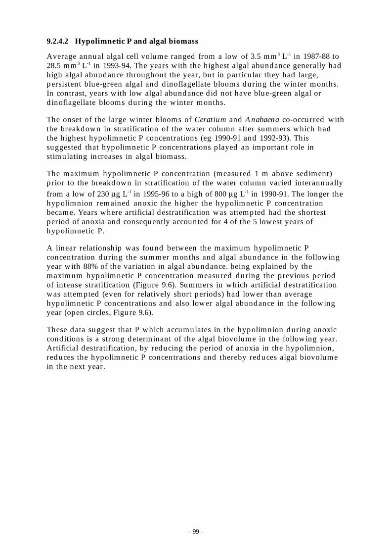
- 99 -

9.2.4.2 Hypolimnetic P and algal biomass

Average annual algal cell volume ranged from a low of 3.5 mm3 L-1 in 1987-88 to28.5 mm3 L-1 in 1993-94. The years with the highest algal abundance generally hadhigh algal abundance throughout the year, but in particular they had large,persistent blue-green algal and dinoflagellate blooms during the winter months.In contrast, years with low algal abundance did not have blue-green algal ordinoflagellate blooms during the winter months.

The onset of the large winter blooms of Ceratium and Anabaena co-occurred withthe breakdown in stratification of the water column after summers which hadthe highest hypolimnetic P concentrations (eg 1990-91 and 1992-93). Thissuggested that hypolimnetic P concentrations played an important role instimulating increases in algal biomass.

The maximum hypolimnetic P concentration (measured 1 m above sediment)prior to the breakdown in stratification of the water column varied interannuallyfrom a low of 230 µg L-1 in 1995-96 to a high of 800 µg L-1 in 1990-91. The longer thehypolimnion remained anoxic the higher the hypolimnetic P concentrationbecame. Years where artificial destratification was attempted had the shortestperiod of anoxia and consequently accounted for 4 of the 5 lowest years ofhypolimnetic P.

A linear relationship was found between the maximum hypolimnetic Pconcentration during the summer months and algal abundance in the followingyear with 88% of the variation in algal abundance. being explained by themaximum hypolimnetic P concentration measured during the previous periodof intense stratification (Figure 9.6). Summers in which artificial destratificationwas attempted (even for relatively short periods) had lower than averagehypolimnetic P concentrations and also lower algal abundance in the followingyear (open circles, Figure 9.6).

These data suggest that P which accumulates in the hypolimnion during anoxicconditions is a strong determinant of the algal biovolume in the following year.Artificial destratification, by reducing the period of anoxia in the hypolimnion,reduces the hypolimnetic P concentrations and thereby reduces algal biovolumein the next year.

- 100 -

0

10

20

30

0.0 0.2 0.4 0.6 0.8 1.0Hypolimnetic TP (mg L-1)

Mea

n A

nnua

l Bio

volu

me

(mm

3 L-1

)y = -3.21 + 35.1x r2 = 0.88

destratifier operated

Figure 9.6 Mean annual algal biovolume vs hypolimnetic TP just prior toturnover at the start of the algal growing year. Open circles denote years that thedestratifier was operated.

9.2.4.3 Algal physiology and bioassays

A number of algal bioassays and in situ physiological assays (NIFT, ∆Φmeasurement; Wood and Oliver 1995, Oliver and Whittington 1998) wereundertaken on samples of algae from the surface layer of Chaffey Dam (Table 9.2).Of the ten algal bioassays undertaken 3 indicated that algal growth was limited bythe availability of nutrient, twice by N and once by P (Feb 1995 - N, Jan 1996 - P,Nov 1996 - N). On one occassion the NIFT assay indicated that phytoplanktonwere limited by the availability of N (Feb 1995), which was in agreement with thealgal bioassay. On the other 2 occasions that bioassays indicated potential nutrientlimitation of growth the phytoplankton did not show any physiologicalsymptoms of nutrient limitation. Measurements of ∆Φ did not clearly indicatenutrient limitation of the phytoplankton community5. On each of the occasionswhen bioassays indicated nutrients were potentially limiting algal growth thewater column was strongly stratified.

Table 9.2 Summary of algal bioassays conducted on 0-3 m integrated watersamples from Chaffey Dam. Nutrient concentrations are of the initial watersample. NIFT refers to a positive result upon the addition of a nutrient (N or P).Bioassay control refers to the percentage increase in fluorescence in the controlflask during the time interval listed. Zero indicates that the control flask did notgrow. Limit nut. is the nutrient most likely to limit algal biomass. Ooc = Oocystis,Chod= Chodatella, Ana = Anabaena, Mer = Merismopedia, Mic = Microcystis, Cer= Ceratium, Sten = Stentor, Volv = Volvox, Bot = Botryococcus.

5 Severe nutrient limitation has been shown to reduce ∆Φ in laboratory cultured algae (Kolber et al.,1988). Other factors, including the previous light history of the phytoplankton can also decrease∆Φ. For the 6 experimental periods ∆Φ was measured to exclude the effects of light, there was noevidence of nutrient-limited reductions in ∆Φ.

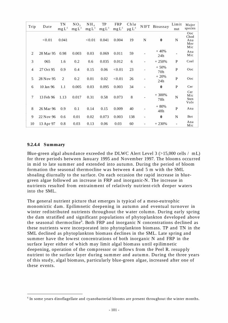
- 101 -

Trip Date TNmg L-1

NO3

mg L-1NH4

mg L-1TP

mg L-1FRP

mg L-1Chlaµg L-1 NIFT Bioassay Limit

nutMajorspecies

<0.01 0.041 <0.01 0.041 0.004 19 N 0 N

OocChodAnaMerMic

2 28 Mar 95 0.98 0.003 0.03 0.069 0.011 59 - + 40%24h - Ana

Mic

3 065 1.6 0.2 0.6 0.035 0.012 6 - + 250% P Coel

4 27 Oct 95 0.9 0.4 0.15 0.06 <0.01 23 - + 50%70h P Ooc

5 28 Nov 95 2 0.2 0.01 0.02 <0.01 26 - + 20%24h P Ooc

6 10 Jan 96 1.1 0.005 0.03 0.095 0.003 34 - 0 P Cer

7 13 Feb 96 1.13 0.017 0.31 0.58 0.073 8 - + 300%78h N

CerMicStenVolv

8 26 Mar 96 0.9 0.1 0.14 0.15 0.009 40 - + 80%48h P Ana

9 22 Nov 96 0.6 0.01 0.02 0.073 0.003 138 - 0 N Bot

10 13 Apr 97 0.8 0.03 0.13 0.06 0.03 60 - + 230% - AnaMic

9.2.4.4 Summary

Blue-green algal abundance exceeded the DLWC Alert Level 3 (>15,000 cells / mL)for three periods between January 1995 and November 1997. The blooms occurredin mid to late summer and extended into autumn. During the period of bloomformation the seasonal thermocline was between 4 and 5 m with the SMLshoaling diurnally to the surface. On each occasion the rapid increase in blue-green algae followed an increase in FRP and inorganic-N. The increase innutrients resulted from entrainment of relatively nutrient-rich deeper watersinto the SML.

The general nutrient picture that emerges is typical of a meso-eutrophicmonomictic dam. Epilimnetic deepening in autumn and eventual turnover inwinter redistributed nutrients throughout the water column. During early springthe dam stratified and significant populations of phytoplankton developed abovethe seasonal thermocline6. Both FRP and inorganic N concentrations declined asthese nutrients were incorporated into phytoplankton biomass. TP and TN in theSML declined as phytoplankton biomass declines in the SML. Late spring andsummer have the lowest concentrations of both inorganic N and FRP in thesurface layer either of which may limit algal biomass until epilimneticdeepening, operation of the compressor or inflows from the Peel R. resupplynutrient to the surface layer during summer and autumn. During the three yearsof this study, algal biomass, particularly blue-green algae, increased after one ofthese events.

6 In some years dinoflagellate and cyanobacterial blooms are present throughout the winter months.

- 102 -

9.3 Light limitation

9.3.1 The underwater light environment

The average light intensity experienced by phytoplankton is dependant upon theincident irradiance, the attenuation of light in the water column and the depth inthe water column of the phytoplankton. In this section we examine the role thatlight may play in regulating algal growth in Chaffey reservoir.

The vertical attenuation coefficient of downwelling radiation (kd) in the watercolumn was measured at Chaffey reservoir on a number of occasions using aLiCor cosine corrected underwater Quantum Sensor (Li-192B). Secchi depths (zSD)were measured weekly at two sites in the dam between 1995 and 1997. There weretwo distinct relationships between attenuation coefficient and secchi depth; oneprior to the dam refilling in late January 1996 and the other from February 1996till April 1997:

k zd SD= +0 239 1 20. . (r2 = 0.59) Feb 1995 to Jan 1996

k zd SD= +0 016 2 45. . (r2 = 0.997) Feb 1996 to Apr 1997

Calibrating the secchi depth data with kd indicates that the euphotic depth,zeu,where 1% of surface light remains ranged from about 1.0 m to 9.5 m with a meanof 3.9 m between 1995 and 1997. During periods when there was a highchlorophyll concentration in the water column the euphotic depth was shallow.

9.3.2 Light dose in the surface mixed layer

Vertical profiles of chlorophyll, in situ fluorescence and cell number have shownthat under most conditions, more than 90% of the phytoplankton resided abovethe seasonal thermocline (Figure 7.2). This suggests that access to light is asignificant determinant of the phytoplankton community structure. To examinethe role of light, it is necessary to compute the typical light dose experienced bythe phytoplankton at different times of years. This is assumed to be directlyproportional to the average daily light intensity in the SML.

Because the SML depth has a strong diurnal variation, the average light intensityexperienced by the phytoplankton has been calculated in two ways. The firstmethod was to calculate the average light intensity over 24 hours using thedeepest SML depth recorded (typically at dawn) in that 24 hour period. Thisapproximates the light climate experienced by an evenly distributed population ofneutrally buoyant algae in the diurnal mixed layer, taking account of the portionof the population that will be stranded at depth as the SML shoals during the day.The second method was to calculate the light intensity averaged over 24 hourswithin the SML (using 10 minute data). This is the light intensity that buoyantand motile algae would experience by remaining in the SML. The results of thesecalculations are shown in (Figure 9.7).

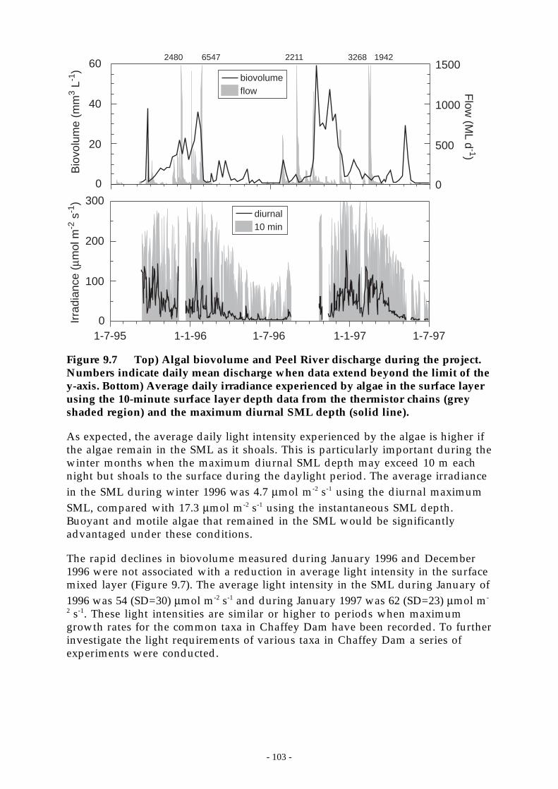
- 103 -

0

20

40

60

0

100

200

300

Irra

dian

ce (

µmol

m-2

s-1

)

1-7-95 1-1-96 1-7-96 1-1-97 1-7-97

Bio

volu

me

(mm

3 L-1

)

2480 6547 2211 3268 1942

0

500

1000

1500

Flow

(ML d

-1)

diurnal10 min

biovolumeflow

Figure 9.7 Top) Algal biovolume and Peel River discharge during the project.Numbers indicate daily mean discharge when data extend beyond the limit of they-axis. Bottom) Average daily irradiance experienced by algae in the surface layerusing the 10-minute surface layer depth data from the thermistor chains (greyshaded region) and the maximum diurnal SML depth (solid line).

As expected, the average daily light intensity experienced by the algae is higher ifthe algae remain in the SML as it shoals. This is particularly important during thewinter months when the maximum diurnal SML depth may exceed 10 m eachnight but shoals to the surface during the daylight period. The average irradiancein the SML during winter 1996 was 4.7 µmol m-2 s-1 using the diurnal maximumSML, compared with 17.3 µmol m-2 s-1 using the instantaneous SML depth.Buoyant and motile algae that remained in the SML would be significantlyadvantaged under these conditions.

The rapid declines in biovolume measured during January 1996 and December1996 were not associated with a reduction in average light intensity in the surfacemixed layer (Figure 9.7). The average light intensity in the SML during January of1996 was 54 (SD=30) µmol m-2 s-1 and during January 1997 was 62 (SD=23) µmol m-

2 s-1. These light intensities are similar or higher to periods when maximumgrowth rates for the common taxa in Chaffey Dam have been recorded. To furtherinvestigate the light requirements of various taxa in Chaffey Dam a series ofexperiments were conducted.

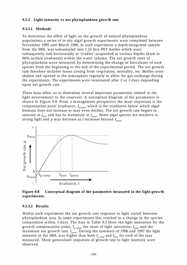
- 104 -

9.3.3 Light intensity vs net phytoplankton growth rate

9.3.3.1 Methods

To determine the effect of light on the growth of natural phytoplanktonpopulations a series of in situ algal growth experiments were completed betweenNovember 1995 and March 1996. In each experiment a depth-integrated samplefrom the SML was subsampled into 1.25 litre PET bottles which weresubsequently laid horizontally in ‘cradles’ suspended at various depths (dark to66% surface irradiance) within the water column. The net growth rates ofphytoplankton were measured by determining the change in biovolume of eachspecies from the beginning to the end of the experimental period. The net growthrate therefore includes losses arising from respiration, mortality, etc. Bottles wereshaken and opened to the atmosphere regularly to allow for gas exchange duringthe experiments. The experiments were terminated after 2 or 3 days dependingupon net growth rate.

These data allow us to determine several important parameters related to thelight environment in the reservoir. A conceptual diagram of the parameters isshown in Figure 9.8. From a management perspective the most important is thecompensation point irradiance, Iµcomp, which is the irradiance below which algalbiomass does not increase or may even decline. The net growth rate begins tosaturate at Iknet and has its maximum at Iµmax. Some algal species are sensitive tostrong light and µ may decrease as I increases beyond Iµmax.

Net

gro

wth

rat

e, µ

Irradiance, I

Iµ comp Iknet Iµmax0

µdark

µmax

+

-

Figure 9.8 Conceptual diagram of the parameters measured in the light-growthexperiments.

9.3.3.2 Results

Within each experiment the net growth rate response to light varied betweenphytoplankton taxa. In some experiments this resulted in a change in the speciescomposition within 3 days. The data in Table 9.3 show the light intensities for thegrowth compensation point, Iµ comp, the onset of light saturation, Iknet, and themaximum net growth rate, Iµmax. During the summers of 1996 and 1997 the lightintensity in the SML was higher than both Iµ comp and Iknet for each of the taxameasured. Three generalised responses of growth rate to light intensity wereobserved.

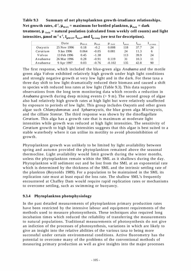
- 105 -

Table 9.3 Summary of net phytoplankton growth-irradiance relationships.Net growth rates, d-1, µµµµMAX = maximum for bottled plankton, µµµµdark = darktreatment, µµµµ field = natural poulation (calculated from weekly cell counts) and lightintensities, µµµµmol m-2 s-1, IµµµµMAX, Iknet, and ΙΙΙΙµµµµ comp (see text for description).

Date µMAX µdark µ field Iµmax Iknet Ι µ comp

Oocystis 25 Nov 1996 0.18 -0.2 0.008 118 37.7 24Ceratium 9 Jan 1996 0.064 -0.05 0.081 24 11.3 6Volvox 13 Feb 1996 0.45 -1.38 113 39.9 24

Anabaena 26 Mar 1996 0.28 -0.91 0.119 31 10.3 11Anabaena 9 Apr 1997 0.03 -0.76 -0.102 135 42.8 90

The first response, which included the blue-green alga Anabaena and the motilegreen alga Volvox exhibited relatively high growth under high light conditionsand strongly negative growth at very low light and in the dark. For these taxa athree day shift to low light dramatically reduced their biomass and caused a shiftto species with reduced loss rates at low light (Table 9.3). This data supportsobservations from the long term monitoring data which records a reduction inAnabaena growth during deep mixing events (> 9 m). The second group of algaealso had relatively high growth rates at high light but were relatively unaffectedby exposure to periods of low light. This group includes Oocystis and other greenalgae such Chlamydomonas and Sphaerocystis, the blue green alga Microcystis,and the cilliate Stentor. The third response was shown by the dinoflagellateCeratium. This alga has a growth rate that is maximum at moderate lightintensities while growth was reduced at high light intensities. The sensitivity ofCeratium growth to high light intensities suggests that this algae is best suited to astable waterbody where it can utilise its motility to avoid photoinhibition ofgrowth.

Phytoplankton growth was unlikely to be limited by light availability betweenspring and autumn provided the phytoplankton remained above the seasonalthermocline. Light availability would limit growth during the winter months,unless the phytoplankton remain within the SML as it shallows during the day.Phytoplankton will sediment out and be lost from the SML at an exponential ratewhich is determined by the thickness of the SML and the intrinsic settling rate ofthe plankton (Reynolds 1989). For a population to be maintained in the SML itsreplication rate must at least equal the loss rate. The shallow SML’s frequentlyencountered at Chaffey Dam would require rapid replication rates or mechanismsto overcome settling, such as swimming or buoyancy.

9.3.4 Phytoplankton photophysiology

In the past detailed measurements of phytoplankton primary production rateshave been restricted by the intensive labour and equipment requirements of themethods used to measure photosynthesis. These techniques also required longincubation times which reduced the reliability of transferring the measurementsto natural populations. Traditional measurements of photosynthesis do not givean indiction of the processes of photosynthesis, variations in which are likely togive an insight into the relative abilities of the various taxa to being moresuccessful under certain environmental conditions. Active fluorometry has thepotential to overcome many of the problems of the conventional methods ofmeasuring primary production as well as give insights into the major processes

- 106 -

of photosynthesis. A key outcome of this project has been to develop the use ofactive fluorometry for freshwater phytoplankton.

9.3.4.1 Methods

The technique of active fluorometry was used to provide information on themajor processes involved in photosynthesis of the commonly occurring algae atChaffey Reservoir including light capture and electron transport through thephotosynthetic apparatus. It measures two parameters, the effective absorptioncross section and the quantum yield of fluorescence. The effective absorptioncross section, σ, is a measure of the size of the antennae (comprised of pigmentmolecules) that the algae use to capture light. The quantum yield of fluorescence,∆Φ, provides a measure of the number of functional photosystem II reactioncentres which is where the light captured by the antennae is converted tochemical energy. In combination these parameters give an estimate of the grossrate of photosynthesis (Kolber & Falkowski 1993, Oliver & Whittington 1998);respiratory losses are not included.

Differences in σ and changes in ∆Φ reflect the conditions under which the algaeare growing. Large σ is hypothesised to occur in algae that grow under low lightconditions where more pigment improves the chances of capturing scarcephotons for photosynthesis. Smaller σ is expected in brigher environments.Changes in σ occur on a time scale of several hours to days. In contrast, ∆Φchanges rapidly (on the order of minutes) in response to changes in the ambientirradiance and more gradually as a result of stress such as chronic nutrientlimitation. Exposure to irradiances above some threshold (roughly 100-120 µmolquanta m-2 s-1 for many terrestrial plants and algae) reduces ∆Φ to below itsmaximum level, ∆ΦM. The amount of reduction increases with increasing lightintensity and duration of exposure. Non-light related stresses, such as nutrientlimitation, that put the algae in a sub-optimal physiological state cause ∆Φ < ∆ΦM

as well.

The photosynthetic rate of a number of the commonly occurring phytoplanktonfound at Chaffey Dam was estimated from the chlorophyll fluorescencemeasurements using the equation proposed by Kolber and Falkowski (1993). Thisrelationship was tested using a number of laboratory cultures. Estimates ofphotosynthesis from fluoresence measurements were compared with directmeasurements of photosynthesis using an oxygen electrode. There was a goodagreement between the two methods (see Oliver and Whittington 1998). Activelyfluorometry was then used to estimate photosynthetic parameters for a numberof key algae in the reservoir.

9.3.4.2 Species-specific photosynthetic parameters

The bloom forming blue-green algae in Chaffey Reservoir generally had smallercross sections than the eukaryotic algae. The exceptions were motile green algae,such as Volvox sp., which under stratified conditions could migrate toward thesurface. Most of the algae measured at Chaffey Reservoir had relatively smallabsorption cross sections compared with estimates in the literature. This resultsupports the hypothesis relating cross section to light environment and indicates

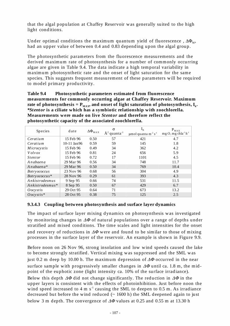
- 107 -

that the algal population at Chaffey Reservoir was generally suited to the highlight conditions.

Under optimal conditions the maximum quantum yield of fluorescence , ∆ΦM,had an upper value of between 0.4 and 0.83 depending upon the algal group.

The photosynthetic parameters from the fluorescence measurements and thederived maximum rate of photosynthesis for a number of commonly occurringalgae are given in Table 9.4. The data indicate a high temporal variability inmaximum photosynthetic rate and the onset of light saturation for the samespecies. This suggests frequent measurement of these parameters will be requiredto model primary productivity.

Table 9.4 Photosynthetic parameters estimated from fluorescencemeasurements for commonly occurring algae at Chaffey Reservoir. Maximumrate of photosynthesis = PMAX, and onset of light saturation of photosynthesis, Ik.*Stentor is a ciliate which has a symbiotic relationship with zoochlorella.Measurements were made on live Stentor and therefore reflect thephotosynthetic capacity of the associated zoochlorella.

Species date ∆ΦMAXσ

Å2 quanta-1IK

µmol quanta m-2 s-1PMAX

mg O2 mg chla-1 h-1

Ceratium 15 Feb 96 0.50 57 421 4.7Ceratium 10-11 Jan96 0.59 59 145 1.8Microcystis 15 Feb 96 0.49 34 362 4.2Volvox 15 Feb 96 0.81 24 656 5.9Stentor 15 Feb 96 0.72 17 1101 4.5Anabaena 29 Mar 96 0.56 34 748 11.7Anabaena* 29 Mar 96 0.50 34 769 10.4Botryococcus 23 Nov 96 0.68 56 304 4.9Botryococcus* 28 Nov 96 0.29 61 393 4.3Ankistrodesmus 9 Sep 95 0.66 74 531 11.5Ankistrodesmus* 8 Sep 95 0.50 67 429 6.7Oocystis 29 Oct 95 0.64 71 673 13.2Oocystis* 28 Oct 95 0.38 75 125 2.5

9.3.4.3 Coupling between photosynthesis and surface layer dynamics

The impact of surface layer mixing dynamics on photosynthesis was investigatedby monitoring changes in ∆Φ of natural populations over a range of depths understratified and mixed conditions. The time scales and light intensities for the onsetand recovery of reductions in ∆Φ were and found to be similar to those of mixingprocesses in the surface layer of the reservoir. An example is shown in Figure 9.9.

Before noon on 26 Nov 96, strong insolation and low wind speeds caused the laketo become strongly stratified. Vertical mixing was suppressed and the SML wasjust 0.2 m deep by 10.00 h. The maximum depression of ∆Φ occurred in the nearsurface sample with progressively smaller changes in ∆Φ until ca. 1.8 m, the mid-point of the euphotic zone (light intensity ca. 10% of the surface irradiance).Below this depth ∆Φ did not change significantly. The reduction in ∆Φ in theupper layers is consistent with the effects of photoinhibition. Just before noon thewind speed increased to 4 m s-1 causing the SML to deepen to 0.5 m. As irradiancedecreased but before the wind reduced (~ 1600 h) the SML deepened again to justbelow 3 m depth. The convergence of ∆Φ values at 0.25 and 0.55 m at 13.30 h

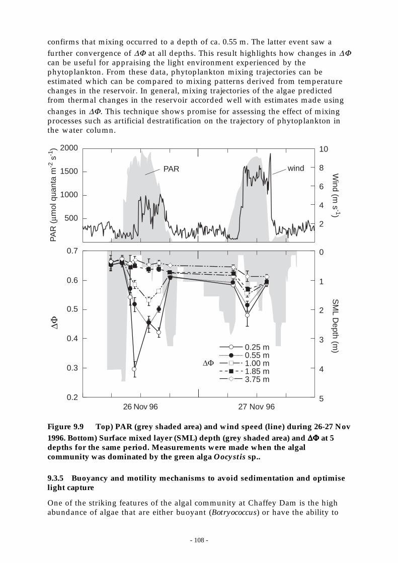
- 108 -

confirms that mixing occurred to a depth of ca. 0.55 m. The latter event saw afurther convergence of ∆Φ at all depths. This result highlights how changes in ∆Φcan be useful for appraising the light environment experienced by thephytoplankton. From these data, phytoplankton mixing trajectories can beestimated which can be compared to mixing patterns derived from temperaturechanges in the reservoir. In general, mixing trajectories of the algae predictedfrom thermal changes in the reservoir accorded well with estimates made usingchanges in ∆Φ. This technique shows promise for assessing the effect of mixingprocesses such as artificial destratification on the trajectory of phytoplankton inthe water column.

∆Φ

26 Nov 96 27 Nov 96

0.25 m0.55 m1.00 m1.85 m3.75 m

5

4

3

2

1

0

2

4

6

8

10

0.2

0.3

0.4

0.5

0.6

0.7

SM

L Depth (m

)W

ind (m s

-1)P

AR

(µm

ol q

uant

a m

-2 s

-1)

500

1000

1500

2000

∆Φ

PAR wind

Figure 9.9 Top) PAR (grey shaded area) and wind speed (line) during 26-27 Nov1996. Bottom) Surface mixed layer (SML) depth (grey shaded area) and ∆∆∆∆ΦΦΦΦ at 5depths for the same period. Measurements were made when the algalcommunity was dominated by the green alga Oocystis sp..

9.3.5 Buoyancy and motility mechanisms to avoid sedimentation and optimiselight capture

One of the striking features of the algal community at Chaffey Dam is the highabundance of algae that are either buoyant (Botryococcus) or have the ability to

- 109 -

migrate vertically in the water column by regulating buoyancy (Anabaena,Microcytis) or by swimming with the use of flagella (Cryptomonads,Dinoflagellates, Stentor, Volvox). These algae accounted for 88% of the total algalbiovolume between 1987-97. Several possible advantages of vertical migrationhave been postulated. These include a reduction in sinking losses, overcomingnutrient limitation by obtaining access to deeper reserves of nutrient andoptimisation of surface light intensity for growth (Harris et al. 1979, Ganf andOliver 1982, Jones 1991).

The success of buoyant blue-green algae in nocturnally mixed waterbodies wherethe maximum diurnal SML depth is much greater than the euphotic depthdepends on the ability of the filament or colony to position itself in a favourablelight climate to satisfy its energy demands when stratification is re-established.The rate of flotation is therefore an important aspect governing the survival ofblue-green algae.

9.3.5.1 Relationship between light, nutrients and buoyancy

Brookes et al. (1999) reported the results of experiments conducted during April1997 at Chaffey Dam that examined the relationships between light, nutrients andcell buoyancy in Anabaena, the dominant blue-green alga in the reservoir.Integrated depth-samples of lake water from 0.2-0.6 m were suspended at dusk on8 Apr 97 in PET bottles at various depths in the water column so that irradiancevaried from 67, 30, 10, 3 and 1 % of the surface irradiance the following day. Someof the bottles also had nutrients added to them as 0.1 mg L-1 P as phosphate and 1mg L-1 N as nitrate. At 08.00 h on 9 Apr 97, all of the Anabaena were positivelybuoyant in all of the samples. By sunset 39% and 9%, respectively, of the uppertwo samples (0.3 m and 0.9 m) which were exposed to high light no longerfloated. At 08.00 h on 10 Apr 97 only 4% of the filaments in the 0.3 m bottle werenot floating and by 17.00 h, 62% and 31% of the 0.3 and 0.9 m samples no longerfloated. The addition of nutrients resulted in an increased resistance to buoyancyloss with only 12% of the 0.3 m sample losing buoyancy by 17.00 on 10 Apr 97. Sixdays later, 0.4 m depth-integrated samples of the natural population taken every0.4 m were also uniformly buoyant at dawn with ca. 30% of the population in thetop 2 m losing buoyancy by 13.00 h and 15% of the population non-buoyant by16.00 h. Two days prior to the latter experiment, the destratifier was turned onand so the ambient conditions within the SML (i.e. nutrient concentrations,stratification, and circulation) in the reservoir had been modified slightly.Nevertheless, the 30% loss in buoyancy in the top 2 m was quite similar to theloss in buoyancy of the 0.9 m bottled sample on 10 Apr 97 (after 2 days).

The light-dependence of the flotation rate of the mixed Anabaena (87%) andMicrocystis (13%) population was studied by suspending samples of lake water inPET bottles at depths corresponding to 70, 30, and 1% of surface irradiance at 10.30h on 14 Apr 97 (Brookes et al. 1999, Table 9.5). The net population flotationvelocity ranged from 0.04 m h-1 (many individual colonies were sinking) fornutrient replete cells held at high light to 2.01 m h-1 for nutrient replete cells heldat very low light for 30 hours. The sinking rate for non-buoyant cells was notdetermined.

The flotation rate of Anabaena was dependent upon the colony size. By 08.00 h on15 Apr 97 differences in carbohydrate content between treatments were not yet

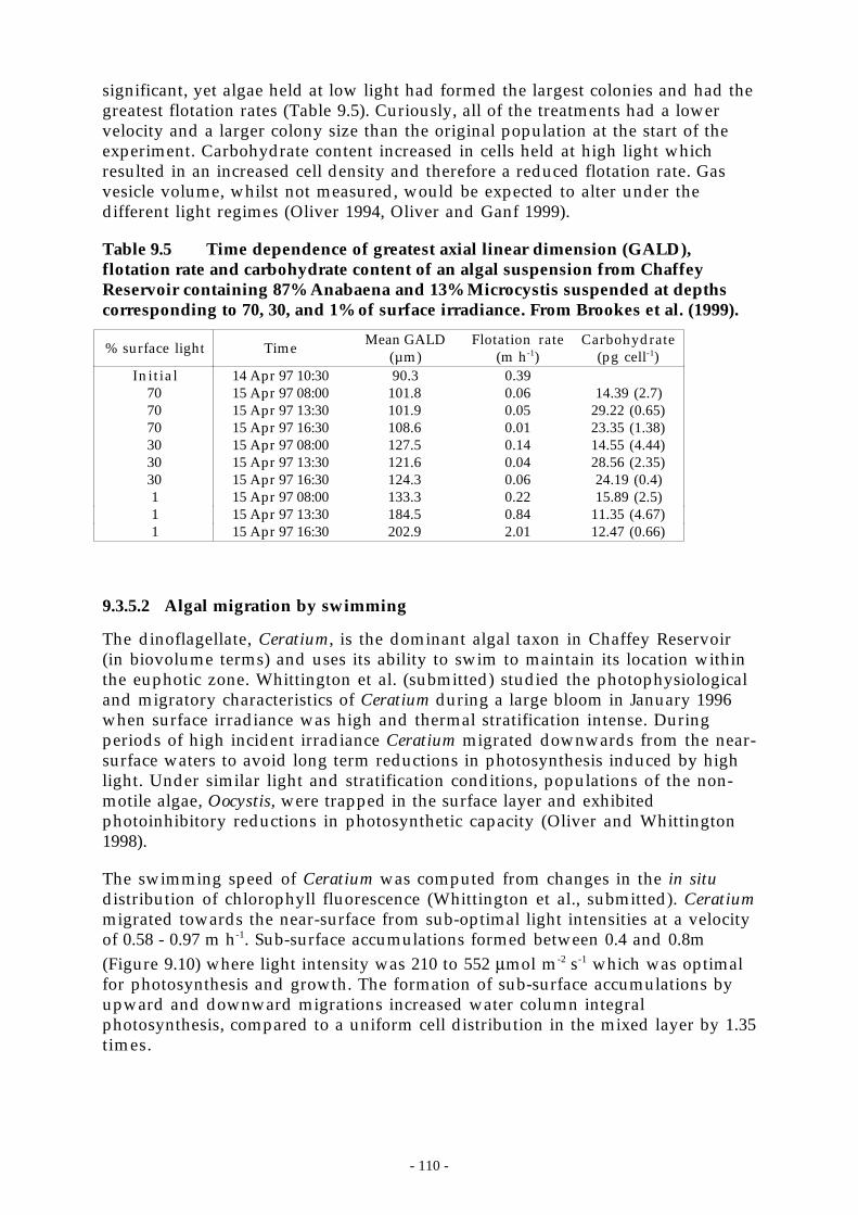
- 110 -

significant, yet algae held at low light had formed the largest colonies and had thegreatest flotation rates (Table 9.5). Curiously, all of the treatments had a lowervelocity and a larger colony size than the original population at the start of theexperiment. Carbohydrate content increased in cells held at high light whichresulted in an increased cell density and therefore a reduced flotation rate. Gasvesicle volume, whilst not measured, would be expected to alter under thedifferent light regimes (Oliver 1994, Oliver and Ganf 1999).

Table 9.5 Time dependence of greatest axial linear dimension (GALD),flotation rate and carbohydrate content of an algal suspension from ChaffeyReservoir containing 87% Anabaena and 13% Microcystis suspended at depthscorresponding to 70, 30, and 1% of surface irradiance. From Brookes et al. (1999).

% surface light Time Mean GALD(µm)

Flotation rate(m h-1)

Carbohydrate(pg cell-1)

Initial 14 Apr 97 10:30 90.3 0.3970 15 Apr 97 08:00 101.8 0.06 14.39 (2.7)70 15 Apr 97 13:30 101.9 0.05 29.22 (0.65)70 15 Apr 97 16:30 108.6 0.01 23.35 (1.38)30 15 Apr 97 08:00 127.5 0.14 14.55 (4.44)30 15 Apr 97 13:30 121.6 0.04 28.56 (2.35)30 15 Apr 97 16:30 124.3 0.06 24.19 (0.4)1 15 Apr 97 08:00 133.3 0.22 15.89 (2.5)1 15 Apr 97 13:30 184.5 0.84 11.35 (4.67)1 15 Apr 97 16:30 202.9 2.01 12.47 (0.66)

9.3.5.2 Algal migration by swimming

The dinoflagellate, Ceratium, is the dominant algal taxon in Chaffey Reservoir(in biovolume terms) and uses its ability to swim to maintain its location withinthe euphotic zone. Whittington et al. (submitted) studied the photophysiologicaland migratory characteristics of Ceratium during a large bloom in January 1996when surface irradiance was high and thermal stratification intense. Duringperiods of high incident irradiance Ceratium migrated downwards from the near-surface waters to avoid long term reductions in photosynthesis induced by highlight. Under similar light and stratification conditions, populations of the non-motile algae, Oocystis, were trapped in the surface layer and exhibitedphotoinhibitory reductions in photosynthetic capacity (Oliver and Whittington1998).

The swimming speed of Ceratium was computed from changes in the in situdistribution of chlorophyll fluorescence (Whittington et al., submitted). Ceratiummigrated towards the near-surface from sub-optimal light intensities at a velocityof 0.58 - 0.97 m h-1. Sub-surface accumulations formed between 0.4 and 0.8m(Figure 9.10) where light intensity was 210 to 552 µmol m-2 s-1 which was optimalfor photosynthesis and growth. The formation of sub-surface accumulations byupward and downward migrations increased water column integralphotosynthesis, compared to a uniform cell distribution in the mixed layer by 1.35times.

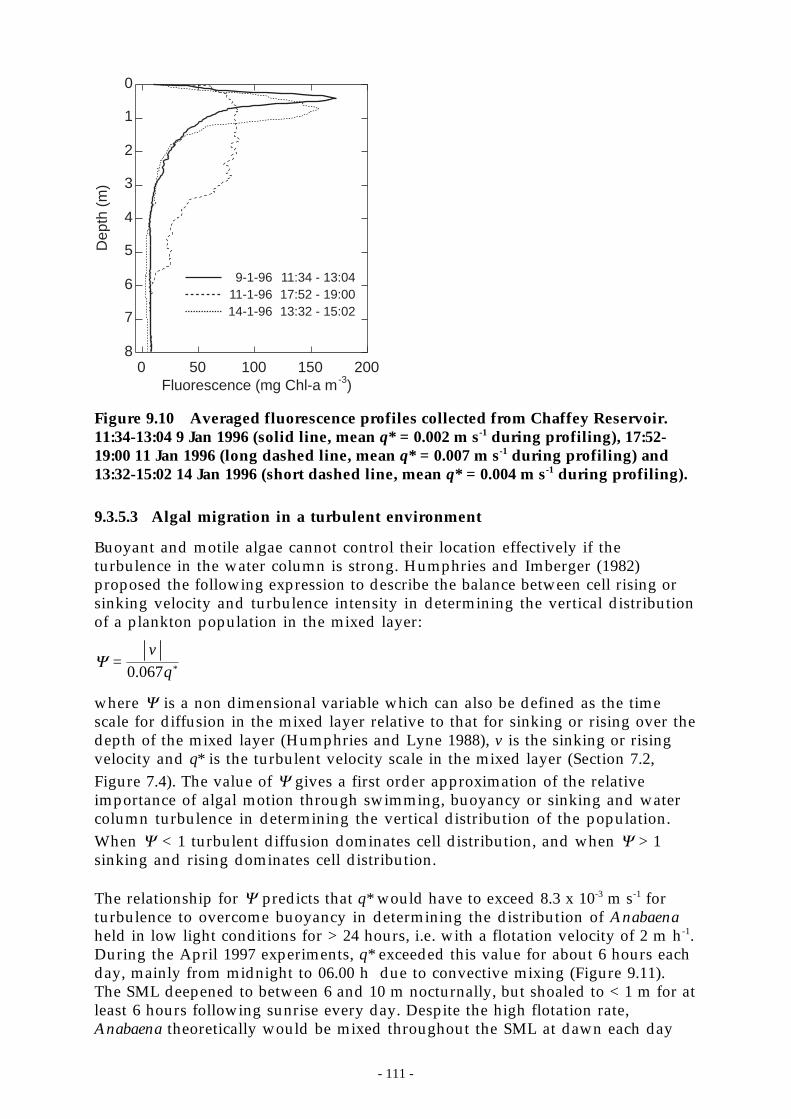
- 111 -

0 50 100 150 200

0

1

2

3

4

5

6

7

8

Fluorescence (mg Chl-a m-3)

Dep

th (

m)

9-1-96 11:34 - 13:0411-1-96 17:52 - 19:0014-1-96 13:32 - 15:02

Figure 9.10 Averaged fluorescence profiles collected from Chaffey Reservoir.11:34-13:04 9 Jan 1996 (solid line, mean q* = 0.002 m s-1 during profiling), 17:52-19:00 11 Jan 1996 (long dashed line, mean q* = 0.007 m s-1 during profiling) and13:32-15:02 14 Jan 1996 (short dashed line, mean q* = 0.004 m s-1 during profiling).

9.3.5.3 Algal migration in a turbulent environment

Buoyant and motile algae cannot control their location effectively if theturbulence in the water column is strong. Humphries and Imberger (1982)proposed the following expression to describe the balance between cell rising orsinking velocity and turbulence intensity in determining the vertical distributionof a plankton population in the mixed layer:

where Ψ is a non dimensional variable which can also be defined as the timescale for diffusion in the mixed layer relative to that for sinking or rising over thedepth of the mixed layer (Humphries and Lyne 1988), v is the sinking or risingvelocity and q* is the turbulent velocity scale in the mixed layer (Section 7.2,Figure 7.4). The value of Ψ gives a first order approximation of the relativeimportance of algal motion through swimming, buoyancy or sinking and watercolumn turbulence in determining the vertical distribution of the population.When Ψ < 1 turbulent diffusion dominates cell distribution, and when Ψ > 1sinking and rising dominates cell distribution.

The relationship for Ψ predicts that q* would have to exceed 8.3 x 10-3 m s-1 forturbulence to overcome buoyancy in determining the distribution of Anabaenaheld in low light conditions for > 24 hours, i.e. with a flotation velocity of 2 m h-1.During the April 1997 experiments, q* exceeded this value for about 6 hours eachday, mainly from midnight to 06.00 h due to convective mixing (Figure 9.11).The SML deepened to between 6 and 10 m nocturnally, but shoaled to < 1 m for atleast 6 hours following sunrise every day. Despite the high flotation rate,Anabaena theoretically would be mixed throughout the SML at dawn each day

Ψ =

v

0.067q*

- 112 -

but by midday all of these colonies would reach the surface where they would beexposed to strong irradiance. Even at the slower flotation speed of 0.84 m h-1 (1%light for 27 hours) the entire population below 4.5 m should still rise fast enoughto ensure an average exposure of ca. 10% of the surface irradiance each day. Itappears unlikely that Anabaena could remain at low irradiances long enough toproduce the higher flotation speeds observed in the bottle experiments at 1%light. This hypothesis is consistent with the natural population’s measuredrising speed of 0.39 m h-1 which suggests an average exposure to between 1 and30% of the surface irradiance.

9 10 11 12 13 14 15 16

SM

L de

pth

(m)

q* (

m s

-1)

0.000

0.005

0.010

0.015

April 1997

0.0

4.0

8.0

12.0

Figure 9.11 Turbulent velocity scale, q*, and SML depth during April 1997. Thehorizontal line in the upper plot is at q* = 8.3 x 10-3 m s-1.

Ceratium were able to form sub-surface accumulations whenever q* < 0.008 m s-1

within the SML. Figure 9.10 shows chlorophyll-fluorescence profiles horizontallyaveraged across the entire reservoir for three quite different meteorologicalconditions (Figure 9.12). On 9 Jan 1996 surface irradiance was low and winds weresufficiently light that q* was just 0.002 m s-1 and the maximum Ceratiumabundance was at 0.4 m. On 14 Jan, q* was 0.004 m s-1, winds were again light butsurface irradiance was much stronger resulting in a deeper fluorescence peak asthe Ceratium moved down to avoid inhibiting irradiances closer to the surface.Ceratium were not able to maintain their position during the afternoon of 11 Jan1996 when a stronger southerly wind of up to 6 m s-1 caused the SML to deepenbriefly to below 2.5 m and Ceratium to accumulate at the northern end of thereservoir. With q* = 0.007 m s-1, Ceratium were evenly distributed above 3 m(Figure 9.10). During the hour prior to profiling q* averaged 0.010 m s-1. Theincrease in fluorescence from 4.5 - 5.75 m depth shows the intrusion caused by theoperation of the destratifier on 11 Jan 1996.

The relationship of Humphries and Lyne (1988) and our measurements ofCeratium swimming speed predict that Ceratium can successfully exploit thestructured, stable epilimnia of the reservoir whilst q* is less than ca. 0.004 m s-1.Generally, the optimum light zone for Ceratium was deeper than 0.4 m, and soalgae below this depth were able to optimize growth by forming aggregationsbelow the SML regardless of q* in the SML when the SML was less than 0.4 m, an

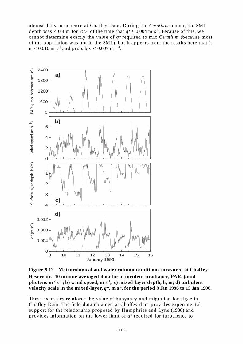
- 113 -

almost daily occurrence at Chaffey Dam. During the Ceratium bloom, the SMLdepth was < 0.4 m for 75% of the time that q* ≤ 0.004 m s-1. Because of this, wecannot determine exactly the value of q* required to mix Ceratium (because mostof the population was not in the SML), but it appears from the results here that itis < 0.010 m s-1 and probably < 0.007 m s-1.

9 10 11 12 13 14 15 16January 1996

q* (m

s-1

)W

ind

spee

d (m

s-1

)PA

R (µ

mol

pho

tons

m-2

s-1

)S

urfa

ce la

yer d

epth

, h (m

)

a)

b)

c)

d)

0

600

1200

1800

2400

0

2

4

6

1

2

3

4

0

0.004

0.008

0.012

Figure 9.12 Meteorological and water column conditions measured at ChaffeyReservoir. 10 minute averaged data for a) incident irradiance, PAR, µµµµmolphotons m-2 s-1 ; b) wind speed, m s-1; c) mixed-layer depth, h, m; d) turbulentvelocity scale in the mixed-layer, q*, m s-1, for the period 9 Jan 1996 to 15 Jan 1996.

These examples reinforce the value of buoyancy and migration for algae inChaffey Dam. The field data obtained at Chaffey dam provides experimentalsupport for the relationship proposed by Humphries and Lyne (1988) andprovides information on the lower limit of q* required for turbulence to

- 114 -

overcome buoyancy or migration in determining the distribution of algae in theSML. This is critical information if the aim is to light limit the growth of thesealgae by artificial mixing.

9.3.6 Sedimentation

In sharp contrast to the high abundance of motile and buoyant algae there wasgenerally a very low abundance of diatoms between 1987 and 1997. Althoughdiatom biovolume was low, diatoms were nearly always present in the watercolumn (Table 9.1). The observed growth of diatoms in unenriched algalbioassays and the growth of a large epiphytic diatom population in associationwith a Cladophora dominated benthic community during the spring (October) of1997 indicates that the water chemistry was suitable for their growth.

That significant diatom populations do not develop except when physicallysupported in the light field indicates that sedimentation may be controlling thegrowth of diatoms at Chaffey Dam. The exponential rate of sinking loss per unittime, ks, of plankton from a continuously mixed layer, hm is given by:

k vhs m= −1

where v is the sinking velocity. If a population is to be maintained in the mixedlayer then loss through settling must be counteracted by growth rate r, such that r- ks remains positive. Settling rates for Aulacoseria and Cyclotella from ChaffeyDam were not calculated but values taken from the literature suggest settlingrates for Aulacoseria in Maude Weir Pool on the Murumbidgee R. of 0.95 m d-1

(Sherman et. al, 1998) and for Cyclotella in Mt Bold Reservoir, SA, of 0.90 m d-1

(Oliver 1981). Given these settling rates and a mixed layer depth of 2 m, thegrowth rate would have to exceed 0.45 d-1 (~doubling every 1.5 days) for thepopulation to increase. This is a high growth rate but should be achievable fornutrient replete populations in Chaffey Dam. This calculation makes theassumption that the diatoms are entrained in a well-mixed surface layer. ForAulacoseria, with a settling rate of 0.95 m d-1, q* would have to exceed 1.6x10-4 ms-1

for entrainment which it does. However, the SML shoals to the surface on mostdays and therefore cells in the euphotic zone but below the SML will clear at thesettling rate, irrespective of the growth rate. If the SML shoaled to the surfacethere would be a loss of ca. 1/3 of the diatom population from the euphotic zoneeach day and replacement would require a growth rate of 1.1 d-1 (doubling time ofca. 0.6 d). This is close to the maximum growth rate under ideal conditions andnot likely to be sustainable in the field.

9.3.7 Can artificial destratification light limit algal growth?

Artificial destratification using the existing equipment in Chaffey Dam is unableto significantly alter the depth of the SML (see section 7.3), however, it doessignificantly weaken the intensity of stratification. This increases the chances of ameteorologically induced deepening of the SML (eg Feb 1996) and probably leadsto a more rapid breakdown in stratification during autumn. However, during thecourse of this study the average light intensity experienced by algae entrained inthe SML was not significantly reduced by the operation of the currentdestratification system.

- 115 -

During periods when the artificial destratification system was operating there wasevidence that algae from the SML were entrained in the bubble plume. Thesealgae then moved horizontally away from the bubble plume in the intrusionbelow the SML. On one occasion that this was observed the dominant alga wasCeratium. The net upward migration rate of Ceratium was ca. 2x10-4 m s-1 and theintrusion entered at ca. 6 m below the surface. At this swimming velocityCeratium initially located in the intrusion was able to re-enter the euphotic zonewithin 4 hours. In a similar fashion, buoyant blue-green algae would float fromthe intrusion back into the SML at a time scale in the order of hours. Theseexamples show that motile and buoyant algae can rapidly re-enter the SML fromthe intrusion associated with bubble plume. Unless the SML is significantlydeepened, entrainment of motile or buoyant algae in the intrusion will notsignificantly reduce the average light intensity experienced by the algalpopulation. Furthermore, in the case of Anabaena, as light limitation is imposedthe rising velocity increases and the minimum q* required to entrain colonies inthe mixed layer increases as well.

To determine the possible effect of artificial destratification on algal growth, theaverage light intensity in the SML was modelled assuming the SML to be held at11 m (artificial mixing) and using meteorological data from September 1995 toNovember 1997. Note that an 11 m SML depth is approximately the mean depthof the reservoir when full and is also approximately 3 times greater than themean euphotic depth of 3.9 m; the latter condition being associated with light-limited growth of Anabaena (Sherman et al. 1998). The mean SML depth cannotexceed the mean reservoir depth so the minimum light exposure of a uniformlydistributed phytoplankton is constrained by the mean reservoir depth. Theaverage light intensities in an 11 m SML during 1996 and 1997 would have been9.4 ± 6.7 µmol m-2 s-1 and 23.6 ± 16.5 µmol m-2 s-1 , respectively, compared to 112 ±88 µmol m-2 s-1 and 134 ± 79 µmol m-2 s-1 calculated using the actual SML depths.The model results imply that if artificial destratification was able to maintain anSML depth of at least 11 m and entrain the phytoplankton then the average lightintensity in the SML would be low enough to limit the growth of algae in ChaffeyReservoir year round (Table 9.3).

9.4 Zooplankton

To investigate the role of grazers in controlling algal abundance in the reservoirzooplankton abundance was determined from 10 m-integrated water samplescollected at 3 sites (A1, A2, A4, Figure 5.1) at the same time as the 5 m-integratedsamples were collected for phytolankton enumeration. A hose was loweredslowly through the top 10 m of the water column while lake water wascontinuously pumped into a bucket. The contents of the bucket were then passedthrough a zooplankton net with a 37 µm filter and preserved in alcohol. Sampleswere collected on 118 dates.

The following observations refer to net zooplankton, consisting of rotifers andmicrocrustacea (cladocerans and copepods). Sampling methods did not permitenumeration or evaluation of the protist component of the Chaffey zooplankton.

- 116 -

9.4.1 Summary & overview

Over the 1995-97 sampling period, 48 taxa of microfauna were recorded from theChaffey Dam zooplankton (30 Rotifera, 12 cladocerans, 5 copepods, 1 ostracod). InAustralia there are few published studies of similar resolution to providecomparison. However, from available data on Australian reservoir zooplankton,the Chaffey assemblage would seem to be at the lower end of the known reservoirspecies richness. In comparison, from only 18 collections over a three year periodin L. Mulwala (Yarrawonga Weir, Murray R., NSW), Shiel (1981) reported 98 taxaof microfauna (67 of rotifers, 21 cladocerans, 8 copepods), from 29 collections inDartmouth Dam over a comparable period, 61 taxa (38 rotifers, 15 cladocerans, 7copepods and 1 ostracod), from eleven collections in Eildon Dam over the sameperiod 48 zooplankton taxa (22 rotifers, 13 cladocerans, 11 copepods and 2ostracods), from 26 collections from Hume Dam over the same period 44 taxa (26rotifers, 10 cladocerans, 8 copepods). Collections from Lyell Reservoir reported byKobayashi (1992b) are not readily comparable in view of the 250 µm mesh sizeused in his 12 mo. study, nevertheless he recorded 10 rotifer taxa, 12 cladoceransand 5 copepods. Similarly, only the microcrustacean zooplankton inWallerawang Reservoir were reported by Kobayashi (1992a), where he recorded 12cladoceran and 3 copepod species.

The same species dominants in the Chaffey assemblage are reported from otherMurray-Darling Basin storages, and appear to be ubiquitous in south-easternAustralia. Bosmina, Ceriodaphnia, Daphnia and Diaphanosoma species are themost common cladocerans, Calamoecia and Boeckella species the commoncopepods. Their population dynamics and seasonal events in Chaffey are broadlysimilar to those reported from other south-eastern Australian reservoirs giventhe constraints imposed by drawdown and catchment-specific human activities(see below).

Zooplankton population densities in Chaffey reservoir are within rangesreported from the above studies, if on the low side for the microcrustaceancomponent. e.g. Kobayashi (1992a) reported a mean of 27.2 ind l-1 formicrocrustacea from Wallerawang, Geddes (1984) reported a range of 35-123microcrustacea l-1 (mean 66 l-1) from L. Alexandrina, Walker & Hillman (1977) arange of 10-60 microcrustacea l-1 from L. Hume. Asplanchna priodonta (Figure9.13) was the most numerous rotifer in the reservoir but there are few publishedrecords of rotifer population densities in Australian reservoirs with which tocompare. Shiel et al. (1987) reported ranges generally less than 200 ind. l-1 inMurray-Darling Basin storages, with occasional pulses of several thousand ind. l-1,and one recorded pulse of 24,000 ind. Synchaeta l-1 in Mt Bold Reservoir, S.A.,apparently in response to a Carteria bloom.

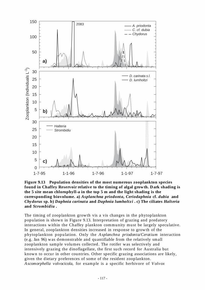
- 117 -

50

100

150

5

10

15

20

25

30

0

5

10

15

20

25

30

a)

b)

A. priodontaC. cf. dubiaChydorus

D. carinata s.l.D. lumholtzi

c)

1-7-95 1-1-96 1-7-96 1-1-97 1-7-97

HalteriaStrombidiu

Zoo

plan

kton

(In

divi

dual

s L-1

)2083

Figure 9.13 Population densities of the most numerous zooplankton speciesfound in Chaffey Reservoir relative to the timing of algal growth. Dark shading isthe 5 site mean chlorophyll-a in the top 5 m and the light shading is thecorresponding biovolume. a) Asplanchna priodonta, Ceriodaphnia cf. dubia andChydorus sp. b) Daphnia carinata and Daphnia lumholtzi . c) The ciliates Halteriaand Strombidiu .

The timing of zooplankton growth vis a vis changes in the phytoplanktonpopulation is shown in Figure 9.13. Interpretation of grazing and predatoryinteractions within the Chaffey plankton community must be largely speculative.In general, zooplankton densities increased in response to growth of thephytoplankton population. Only the Asplanchna priodonta/Ceratium interaction(e.g. Jan 96) was demonstrable and quantifiable from the relatively smallzooplankton sample volumes collected. The rotifer was selectively andintensively grazing the dinoflagellate, the first such record for Australia butknown to occur in other countries. Other specific grazing associations are likely,given the dietary preferences of some of the resident zooplankton.Ascomorphella volvocicola, for example is a specific herbivore of Volvox

- 118 -

colonies. It was present in the Chaffey zooplankton only when Volvox waspresent. Some rotifers (e.g. Gastropus, Synchaeta), selectively prey on monads andwere present in the Chaffey zooplankton when the preferred food item wasabundant. Bacteriovores, e.g. Conochilus, Filinia, Hexarthra, Pompholyx, et al.although generally in low numbers, provide evidence of bacteriovory in theplankton community.

The microcrustacean assemblage in Chaffey is problematic in that only smallspecies were abundant; larger-bodied zooplankton such as Daphnia andBoeckella, which predominate in other reservoirs, were not present in largenumbers, or were markedly seasonal. Fish predation was invoked by Kobayashi(1992b) to explain a similar size shift in both Lyell and Wallerawang reservoirs.Both reservoirs were stocked with planktivorous fish, such as brown andrainbow trout. Possibly, some food chain effect is operating on the Chaffeyzooplankton community, but in the absence of fish species information, density,stocking, etc. data, it is not possible at this point to determine if fish are depletingthe larger herbivorous zooplankton.

Circumstantial evidence points also to invertebrate predation structuring theChaffey zooplankton - large numbers of juvenile shrimp, which areplanktivorous, were noted in settling trap samples. These may be seasonal orperennial predators of larger zooplankton. Notonectids and other carnivorousaquatic stages of insects may also structure zooplankton communities, howeverevidence for their activities in Chaffey is lacking.

Intuitively, it is likely that the smaller (rotifer) component of the Chaffeyzooplankton is structured by the numerically dominant nauplii/copepoditestages of Thermocyclops, the size preference and food item choice of whichchanges with maturity. The calanoid Calamoecia, notably one of the smallestcentropagids, probably is omnivorous in juvenile stages, preying on ciliates,rotifers, and smaller instars. High mortality of copepods in Chaffey, as suggestedby low density of adults, despite juveniles usually being the most abundantzooplankters present, implies predation by a visual predator(s). Largerzooplankters in Chaffey also appear to be depleted by predation, possibly as aresult of the fish stocking that occurs at the dam.

9.5 Summary

During the springs of 1994, 95 and 96 biological consumption of FRP andinorganic-N in the SML reduced the concentration of these nutrients to levelslimiting algal biomass. At the same time, nutrients were accumulating in thehypolimnion. When commenced in summer, the short-term effect of artificialdestratification was to inject nutrients into the SML which then led to an increasein algal biomass, particularly Anabaena and Microcystis.

In the long term, oxygenation of the hypolimnion by artificial destratificationreduced the internal release of P from the sediments. There is clear evidence thatthe years in which artificial destratification was attempted had the shortestperiods of anoxia in the hypolimnion and the lowest concentrations ofhypolimnetic P. Since the hypolimnetic P concentration strongly determines thefollowing year’s algal biomass, operation of the destratification system does

- 119 -

reduce the average annual algal biomass. However, blooms of blue-green algaestill occurred even in the years with the lowest hypolimnetic-P.

The inability of the destratifier to deepen the SML prevented it from reducing theavailability of light sufficiently to stop blooms of blue-green algae. Theoreticalcalculations using the growth-irradiance curves for the phytoplankton in thereservoir suggest that for light to become limiting an SML depth of 11 m must bemaintained. This is close to the average depth of the reservoir when full. Becauseof the broad expanses of shallow water in the southern part of the reservoir, itseems unlikely that light limitation will be an effective strategy to control blue-green algal blooms in Chaffey Dam.

Furthermore, because the flotation speed of Anabaena increases with lightlimitation, the q* required to distribute them throughout the SML increases aswell. Climatic conditions may not be capable of maintaining a sufficient level ofturbulence in the water column.

- 121 -

10 Management implications

The strong correlation between hypolimnetic TP and the following year’s averageannual algal biovolume suggests that algal control strategies focusing on reducingthe supply of phosphorus to the water column are most likely to provide shortterm benefits. Being similar in magnitude, both external and internal sourcesneed to be addressed as reduced external loading will not improve the algalbloom problem during drought years. Conversely, reduced internal loads mayprovide only a small improvement during normal-to-wet years when thecatchment delivers very high quantities of FRP.

Although the algal physiological data suggest that light limitation of algal growthis theoretically possible, destratification within the time scale required to deepenthe surface mixing layer sufficiently to achieve this is likely to prove very costly.Using a conventional bubble plume destratifier, the air flow rate would probablyneed to be increased from 100 L s-1 to at least 1300 L s-1and probably more (Section4.2.2). The pipe network would have to increase in size vastly as the number ofindividual plumes increases from 10 to more than 100, ideally with at least 30 mseparation between plumes.

A rough idea of the cost of a new bubble-plume destratification system can beextrapolated from the experience of the South East Queensland WaterCorporation who in the late 1990’s installed a state-of-the-art system with anairflow rate of 400 L/s at North Pine Dam. This system had a capital cost of$400,000 and currently costs approximately $100,000 per annum to operate. Thecost of a new system should scale roughly linearly as the ratio of airflow ratesbetween the new and North Pine systems, i.e. a 1300 L s-1 system would have acapital cost of roughly $1.2m and and operating cost of $300,000 per annum.

Below, we describe briefly operational considerations regarding artificialdestratification, nutrient reduction strategies, and a speculative method for light-limiting algal growth.

10.1 Operational considerations for artificial destratification

10.1.1 Effects of the destratification system on water column chemistry

Destratification provides an effective means of increasing hypolimnetic oxygenconcentrations and thereby reducing sediment nutrient releases. The downwardmixing of oxygenated waters into the hypolimnion rapidly reduces theconcentrations of hydrogen sulphide and reduced iron and manganese and alsofacilitates scavenging of FRP by increasing the supply of Fe(OOH). Within theformer hypolimnetic zone oxygen becomes the electron acceptor rather thansulphate at the sediment surface, and sulphate reduction will only occur inanoxic areas deeper within the sediment. Essentially, the exposure of thesediments to oxygen will change the bacterial population from anerobic to aerobicpopulations and thus stop the anerobic route for release of nutrients into thewater column.

It is essential that operation of the destratifier commences before largeconcentrations of nutrients are allowed to accumulate in the hypolimnion.Otherwise, it provides an effective means of transporting these nutrients into the

- 122 -

surface layer where they can be utilized to fuel algal growth. If commencement ofdestratification is delayed until after significant quantities of reduced chemicalspecies and organic carbon accumulate in the water column, the short-term effectmay be to further exacerbate anoxia throughout the water column (Section 8.3.7).Furthermore, any reduction in the SML O2 concentration may retard nitrificationand denitrification, shifting the distribution of inorganic nitrogen species. Thishas implications for the balance of species in the euphotic zone.

Destratification clearly can reduce sediment nutrient release, but it also retardsthe loss of nutrients from the surface by sedimentation. The decision to destratifymust weigh the benefits of decreased internal nutrient loading against potentiallyhigher mean nutrient concentrations during the summer growing season.

10.1.2 Thermal effects of destratification

When the destratifier is operated the temperature of the hypolimnion isincreased by about 10 °C. The increased temperature increases the rates of all ofthe biologically mediated reactions, especially the consumption of O2 by thesediments and within the water column. Our measurments demonstrated thatwater column BOD increased by a factor of 2.7 for a 10 °C temperature increase.This has profound implications for the oxygen budget of the reservoir. Thesupply of oxygen across the air-water interface plus the in situ production byphotosynthesis must meet the demand for oxygen in the warmer reservoir. If thesupply of oxygen doesn’t match the downward transport and consumption, thendestratification can actually reduce the total amount of oxygen in the watercolumn.

Once destratification commences it must continue throughout the stratificationseason as the increased hypolimnetic temperatures will accelerate thedevelopment of anoxia and the ensuing release of phosphorus from thesediments in the event of the destratifier being turned off.

10.2 In-reservoir phosphorus reduction strategies

10.2.1 Selective withdrawal from the hypolimnion

Selectively releasing water from the hypolimnion removes nutrients from thewater column before they can reach the surface layer. The disadvantages includethe smell of H2S in the vicinity of the outlet and possible problems withmanganese deposition for down stream users of water taken from the river.

The relatively small quantities of water released from the dam under normalconditions may limit the effectiveness of this option due to insufficient removalof accumulated nutrients from the hypolimnion.

10.2.2 Destratification

By reducing the internal nutrient load, continuous (August – May) operation ofthe destratification system is likely to reduce the average algal biomass in the dambecause there will be less nutrient supplied to the SML from the hypolimnionduring epilimnetic deepening. It is also likely to reduce the intensity and

- 123 -

duration of blue-green algal blooms because it brings forward the date of initialoverturn of the water column.

Destratification will not completely eliminate the growth or formation of blue-green algae because the Peel R. can deliver quantities of nutrient to the reservoirsufficient to stimulate algal blooms (for example Feb 1997). These inflows arehigh in NO3 relative to NH4 and therefore likely to stimulate the growth ofAnabaena rather than Microcystis. Because the major inflows typically intrudebelow the SML (section 7.1), the phytoplankton population will not respond tothe associated nutrient load until the SML deepens enough to entrain water fromsuch an intrusion.

Operation of the destratifier will likely increase transport of nutrients from aninflow intrusion to the SML thereby promoting algal growth. Discontinuing theoperation of the destratifier in order to prevent this transport of nutrients willresult in anoxia in the hypolimnion within 30-60 days and the resumption of theassociated internal nutrient load. The internal nutrient load will increase theaverage algal biomass experienced during the following year. Clearly, operation ofa destratifier during years with significant spring or summer inflows is acomplicated issue that is particularly sensitive to the timing and chemistry ofinflow events.

10.2.3 Hypolimnetic oxygenation

Hypolimnetic oxygenation involves directly injecting pure oxygen or compressedair into the hypolimnion. The latter method is often referred to as ‘aeration’.Oxygen is dissolved directly into the hypolimnetic water to reduce the nutrientrelease from the sediments while at the same time not disturbing the thermalstratification. Preserving the stratification allows nutrients to be lost from theSML through particle sedimentation and slows the upwards transport ofdissolved nutrients from the hypolimnion to the SML. The elevated oxygenconcentration reduces sediment nutrient release.

Hypolimnetic oxygenation has the potential to decrease average annual biomassand summer-autumn biomass more than destratification. Allowing a springphytoplankton bloom reduces SML nutrient concentrations to limiting levelswhen the bloom species subsequently sediments out of the SML. This will resultin very low chl-a concentrations in summer and autumn. Hypolimneticoxygenation will prevent the subsequent remobilization of sediment nutrientsthereby reducing the resupply of nutrients to the SML during autumnaldeepening.

There are several oxygen delivery systems used in different reservoirs around theworld. Two main approaches are used: injection of pure oxygen gas through adiffuser (e.g. ‘seeper hose system’ developed by the Tennessee Valley Authority);and injection of water previously supersaturated with oxygen in a special mixingchamber (e.g. Speece Cone or Vitox™ systems). The appropriate system for aspecific reservoir depends particularly on the reservoir’s depth. Direct injection ofoxygen gas performs best in deeper reservoirs where dissolution of the oxygeninto hypolimnetic waters is maximised by longer contact times as the bubbles risethrough the hypolimnion. In shallower reservoirs where bubble contact time is

- 124 -

limited, a Speece Cone or Vitox system may be required to efficiently deliver theoxygen.

Hypolimnetic aeration in which compressed air released through a diffuser in thehypolimnion provides the oxygen source may be an attractive option, especiallyfor shallow reservoirs (depth < 10 m). A special chamber is used to confine theeffect of the bubbles to the hypolimnion so that the thermocline is not disturbed.The city of Norfolk, Virginia, uses this technique to control iron and manganesein their water supply reservoirs.

We can provide a rough estimate of the cost to oxygenate Chaffey Reservoir usinga seeper hose system using the oxygen demand figures from section 8.3.7. Theseeper hose system is attractive in that it has no moving parts – it is poweredentirely by the expansion of liquid oxygen to gaseous oxygen – and should offergreater reliability as compared to compressor-based systems. The capital andoperating cost estimates have been extrapolated from a similar calculation madefor the 167,000 ML Hinze Dam (Gold Coast, QLD) and are indicative only. Themedian areal oxygen demand in Chaffey Reservoir from 1992-1997 was 0.55 x 10-3

kg O2 m-2 d-1. Assuming the top of the anoxic region is at an elevation of 506 m

(i.e. the reservoir is full) gives a sediment area of 248 ha and a hypolimneticoxygen demand of 1364 kg d-1. Assuming a factor of safety of 3x gives a designoxygen supply rate of roughly 4000 kg d-1. The Hinze Dam system had a designoxygen supply rate of 15,000 kg d-1 with estimated capital cost of $1.5m andoperating costs of $3000 d-1. Assuming the cost scales linearly with oxygen supplyrate and that the system operates 210 days per year gives for Chaffey Reservoir acapital cost of $500,000 and an annual operating cost of $168,000. Continuousoperation for 210 days of the existing compressor at Chaffey Reservoir costsapproximately $145,000 for power alone. These figures suggest that hypolimneticoxygen may be a financially attractive alternative to conventional bubble-plumedestratification.

10.2.4 Sediment remediation

Sediment remediation will greatly reduce the remobilisation of nutrients fromthe current dam sediments. Possible remediation strategies include: dredging;injection of the sediments with CaNO3 (the Riplox method); and capping with anengineered clay such as Phoslock™. However, subsequent external loads ofsediments to the dam via the Peel River will replace the treated sediments as thesource of nutrients and require further remediation. This option is not viableunless a significant reduction in the external sediment load can be effected.

To cap with Phoslock the 240 ha of sediments regularly exposed to anoxicconditions would cost approximately $xxx,xxx.

10.2.5 Fe3+ dosing

Further reductions in water column FRP, and therefore average annual algalbiomass, may be achieved by increasing the supply of amorphous FeOOH giventhat there is insufficient Fe2+ to scavenge all the FRP in the water column. Thiseffect could be achieved by adding Fe3+ to the water column either throughinjection via the bubble plume or by distribution across the surface of the damreservoir. Note that it is necessary to maintain oxic conditions throughout the

- 125 -

water column, by either destratification or hypolimnetic oxygenation, in order forthis strategy to be effective. Iron dosing also may have to be repeated followingthe arrival of large external nutrient loads.

10.2.6 Sediment dessication and oxidation as control strategies for P release

As noted earlier (Section 8.2.7) this project has shown that sediments subject toprolonged exposure to air and drying suffer a decrease in the capacity to release Pon rewetting and being subjected to anoxia. The duration of this effect willdepend on the time required for bacteria to recolonize the sediments uponreinundation. This finding opens up opportunities to moderate P release inreservoir systems were there is scope to lower water levels and expose sediments.

Historically, Chaffey Reservoir has been operated to maintain the reservoir in afull or nearly full condition (Figure 6.4b). Assuming that only the sedimentsbelow 506 m (i.e. depth > 12 m) are regularly exposed to anoxic conditions andthereby provide a significant source of P (section 10.2.3), dessication of 50% of thesediment area below 506 m would require drawing the reservoir level down to501.5 m, i.e. just 7% of capacity. Given that the average annual inflow to thereservoir is 22,200 ML, the reservoir may not fill again for several years posing anunacceptable risk to supply for downstream users.

10.3 Catchment management

Catchment delivery of nutrients, in particular FRP and SO4, is a significantcontributor to the algal growth problem at Chaffey Reservoir. Identification of thesources of inorganic nutrients, particularly FRP and SO4 is essential prior to theimplementation of any large scale catchment management changes. This willrequire monitoring of flows and in-stream chemistry using stage-dependentsamplers on the major tributaries to the Peel River upstream of Taroona.

10.3.1 Control of sulphate entry into the Dam.

Considerable quantities of sulphate enter the dam during major flood events.Earlier work by Donnelly (1994) showed that the sulphate in the sediments hadan δ34S consistent with the source of sulphate being derived from the principalvariety of fertiliser applied in the catchment. While some more recent work(Candace Martin, unpub.) supports this proposition, our work suggests that theremay be an additional non-fertiliser source. The sulphate concentration in theDam varies between 15 and 25 mg L-1 depending on the season and the antecedentinflows. While this concentration is not sufficient to cause a significant increasein the rate of nutrient generation (Caraco et al, 1993), it is a major electronacceptor. In terms of oxidising capacity it is equal to, or perhaps surpasses, thedissolved oxygen content of the dam, with 2 moles of organic matter (nominallyCH2O) broken down per mole of sulphate. The significant drawdown in sulphateconcentration once the dam has stratified and its return to the originalconcentration after the autumnal overturn (Figure 8.6) are good evidence for itsactive involvement in the diagenic processes.

Lessening the sulphate concentration reduces the amount of sulphide producedunder anoxic conditions in the water column. This would:

- 126 -

• reduce the chemical oxygen demand during overturn of the hypolimnion

• decrease sulphide reduction of FeOOH and the concomitant release ofadsorbed phosphate

Donnelly (pers. com.) advocates the replacement of the gypsum in the standardfertiliser with elemental sulphur which would lead to a slower release of thephosphate in the fertiliser and a reduction in the external sulphate load to thereservoir. Sulphate reduction appears to “switch off” at a concentration of about10 mg L-1 which seems to be a reasonable target to aim for in the storage.

10.4 Light limitation strategies

10.4.1 Surface impellers to light-limit algal growth

Using impellers to pump surface layer water down below the thermocline mayprovide an alternative strategy to light-limit algal growth. In this scenario,impellers are designed to pump a known proportion of the surface layer, say 20%of the top 5 m of the water column per day, down into or below the thermocline.The idea is to decrease the residence time within the surface layer significantly,thereby producing a more dynamic light regime less suitable for buoyantcyanobacteria. At present it is not known to what depth the surface-layer watermust be delivered to prevent buoyant cells rising back into the SML in time toresume normal growth.

Low velocity impellers used in combination with a draft tube can move largequantities of water at a much lower cost than either bubble plume orconventional mixer systems. However, this method is highly speculative atpresent and unresolved issues include hardware reliability, public access, liabilityand the number of impellers required. The CRC for Water Quality and Treatmentis currently undertaking a trial of surface impellers at both Myponga and HappyValley reservoirs in South Australia.

- 127 -

11 Appendix A – Destratification experiments

11.1 The effect of Artificial mixing on phytoplankton abundance and communitycomposition.

Between February 1995 and April 1997 the compressor at Chaffey Dam wasoperated for 5 periods of between 11 and 36 days. Artificial mixing wasundertaken at different times of the year, with different water column chemistryand thermal structure and with different initial phytoplankton abundance andcommunity structure. The changes in algal community structure and biomassoccurring at the times when artificial destratification was attempted aresummarised in Table 4 and described below.

11.2 Trial 1. 22 Feb 95 to 29 Mar 95

Prior to the commencement of artificial destratification in late February 1995 thereservoir was strongly stratified with low concentrations of inorganic N (<0.02mgL-1) and FRP (0.004 mgL-1) in the surface layer and very high concentrations ofFRP (0.415 mgL-1) in the anoxic hypolimnion. Chlorophylla concentration ( [Chla]) in the surface layer was 20 µg L-1 and the algal community was comprised ofAnabaena circinalis, Oocystis sp. and Cryptomonas sp.. Whilst there was a lowconcentration of FRP in the surface water, algal bioassays and in situ physiologicalassays (Wood and Oliver 1995) both indicated algal growth to be limited by theavailability of N. Destratification resulted in a rapid increase in the concentrationof FRP in the mixed layer and over a 35 day period of destratification [Chla]doubled and the algal community became dominated by the N-fixing blue-greenalga, Anabaena circinalis. Anabaena persisted at a high abundance for 4 weeksafter aeration ceased. This trial reinforces the requirement to understand what islimiting the growth of algae prior to artificial mixing, since mixing is most likelyto increase algal growth in nutrient limited water bodies.

11.3 Trial 2 4 Oct 95 to 28 Oct 95

During the 2 weeks leading to the commencement of artificial mixing the diurnalmixed layer was between 2 and 4m, there was sufficient N and P to support algalgrowth (check this statement!) and chla concentration was increasing. Thephytoplankton community was dominated by the green algae, Oocystis. Duringthe 25 days of compressor operation the chlorophyll concentration did notsignificantly alter (12.7 ±6.3 µg L-1) and Oocystis remained the dominantphytoplankton. Oocystis concentration doubled in the month after thecompressor was turned off.

11.4 Trial 3 11-1-96 to 13 Feb 96

Prior to the commencement of artificial mixing there was a large population ofthe migratory dinoflagellate, Ceratium in the relatively shallow mixed layer priorto operation of the destratifier. Within 12 days of compressor operation there wasa dramatic decline in the abundance of Ceratium which was reflected in surfacelayer [Chla] declining from 38.7 ±31.8 µg L-1 (SD n=5) on 16-1-96 to 1.9 ±1.0 µg L-1

(SD n=5) on the 23-1-96. The very high CV was due to the extreme horizontalheterogeneity in Ceratium abundance. The spectacular decline in [Chla] was

- 128 -

coincident with the onset of artificial mixing. However, the decline in Ceratiumabundance was the direct result of intensive grazing by the rotifer, Asplanchnapriodonta. [Chla] remained low during the remaining period of destratificationbut did increase during February with the growth of Cryptomonas and thedinoflagellate Peridinium. During the last week of compressor operationMicrocystis aeruginosa and Anabaena circinalis appeared in the mixed layer andbecame the dominant algae during March and April.

11.5 Trial 4 24 Nov 96 to 24 Dec 96

Artificial destratification was attempted in late November 1996. Chlaconcentration in the mixed layer was 139 ±46 µg L-1 and the phytoplankton wasalmost exclusively dominated by the buoyant, colonial green algae, Botryococcus.There was a strong thermocline at ca. 4m with an anoxic hypolimnion. Mixedlayer inorganic N (0.03 mg L-1) and FRP (0.003 mg L-1) concentrations were lowand bioassay results indicated that phytoplankton growth was potentially limitedby the availability of N. During the period of artificial mixing Chla concentrationdeclined steadily to less than 10 µg L-1 after 30 days. Botryococcus disappearedduring the period of artificial mixing and was replaced by low numbers ofCeratium and Oocystis.

11.6 Trial 5 13 Apr 97 to 23 Apr 97

Artificial destratification was attempted in mid April as the epilimnion wasdeepening. Algal bioassay results indicated that prior to the commencement ofartificial mixing there was sufficient nutrient (inorganic N 0.16 mg L-1 ; FRP 0.03mg L-1) in the mixed layer to support phytoplankton growth. A bloom ofAnabaena which peaked between 1-8/4/97 at ca. 69000 cells mL-1 had declined bythe commencement of destratification to ca. 3500 cell mL-1 and continued todecline during artificial mixing. Chl remained low but the Anabaena wasreplaced by crytomonads and Peridinium, which continued to increase afterartificial mixing ceased.

11.7 Conclusions of short term mixing

The operation of the artificial mixing system at Chaffey Dam did not result in asystematic change in either phytoplankton abundance or composition. With thecurrent compressor installed in Chaffey Dam the most likely short term outcomeof its operation is to not affect phytoplankton abundance or communitycomposition. However, if there is a nutrient limited phytoplankton populationin the mixed layer and sufficient nutrient is transported from the hypolimnion tothe mixed layer it is likely that this will result in an increase in algal growth. Theincrease in Anabaena and Microcystis abundance observed during the first trial isan example of this.

- 129 -

12 Appendix B - Zooplankton observations by year

12.1 12 Sep 95 – 26 Dec 95 (n=17 dates x 3 sites)

Rotifera were rare in the sampling period. Nine taxa of Rotifera were recorded.With the exception of the omnivorous Asplanchna priodonta, all were at lowdensities - one or a few individuals per litre, and of negligible significance interms of numbers or biomass. A. priodonta pulsed briefly for two weekscoincident with it’s preferred food item, the dinoflagellate Ceratium. A similarlysmall pulse of a bacteriovore, Filinia longiseta, occurred over two weeks in Oct.-Nov., however at a maximum density of ca. 22 ind. l-1 this represents negligiblebiomass. Filinia is <200 µm body size.

Nine taxa of planktonic cladocerans were recorded, only one of which,Ceriodaphnia cf. dubia was persistent in appreciable numbers at all three sites.Daphnia lumholtzi and Diaphanosoma unguiculatum probably were presentthroughout the sampling period, but were in such low numbers or patchilydistributed that they were not collected on every sampling occasion, or at everysite. When they were collected they were in low numbers, generally only one or afew individuals per litre. All three taxa are small, <1 mm. Larger herbivorouscladocerans, e.g. Daphnia were notably absent during this period.

Copepoda were numerically dominant during the 1995 sampling period,primarily as nauplii and copepodites of the small centropagid Calamoecia lucasi,or of the cyclopoid Thermocyclops sp. Notably, occasional pulses of egg hatchingand nauplius production were not reflected by population increases inCalamoecia/Thermocyclops late instar copepodites or adults in succeeding weeks- the juveniles did not survive to maturity.

During the 1995 sampling period, mean zooplankton densities at the three siteswere low: Site 1: 112 ind l-1; site 2: 126 ind. l-1, site 4: 178 ind. l-1.

12.2 02 Jan 96 – 30 Dec 96 (n=52 dates x 3 sites)

Low diversity of Rotifera throughout 1996 was a feature of all three sites. Of 14rotifer taxa identified, only one, Asplanchna priodonta, reached high densities(>4000 ind. l-1) again coincident, or with a slight lag following, the dinoflagellateCeratium. Gut content analysis of A. priodonta during the Jan.-Feb. pulsedemonstrated that it was grazing primarily or exclusively on Ceratium. Hexarthramira, a bacteriovore/detritivore, probably was persistent throughout summer-autumn, but was collected only intermittently, as one or a few individuals perlitre, and rarely was concurrent at all three sites. Rotifers were notably absentfrom all three sites June-Dec.

Eleven taxa of cladocerans were recorded over the 12 mo. sampling period, noneof them perennially. C. cf. dubia was again the most abundant cladoceranplankter, with late-summer/spring maxima. It was not recorded at all May-Nov.Daphnia carinata s.l. and Diaphanosoma unguiculatum probably overwintered insmall numbers - individuals appeared sporadically in samples May-Sept. D.carinata s.l.¸ the largest herbivore present, reached appreciable numbers for only

- 130 -

three weeks in Feb. (max. <20 l-1). Also sporadic in low numbers were Bosminameridionalis (Jan.-Apr.), Ceriodaphnia cornuta (Mar.-Apr.). Chydorus sp., adetritivore/bacteriovore, appeared Oct-Dec., was the second most abundantcladoceran during this period.

Of the four taxa of Copepoda recorded over the 12 mo. period, both Calamoecialucasi and Thermocyclops sp. probably were perennial, again primarily asjuveniles. They were present on most sampling dates, although not at all sites,and in low numbers May-Dec. With the exception of the pulse of Asplanchnapriodonta in Jan., juvenile copepods were numerically abundant Jan-May. Theypersisted in low numbers over winter, but did not recover dominance in theSept.-Dec. period, when the group of cladoceransCeriodaphnia/Daphnia/Chydorus were numerically dominant. Again, the lownumbers of adults of both Calamoecia and Thermocyclops, generally occurring asonly a few individuals per litre, suggest that mortality of juvenile stages washigh. Notable also was the infrequent occurrence of the larger centropagidcalanoid grazers, Boeckella fluvialis and B. triarticulata. One or the other specieswas recorded intermittently as one or two individuals during Feb.-Dec.,suggesting that Boeckella could well have been perennial over the study period,but in such low numbers or patchy distribution that it was not sampled.

During the 1996 sampling period, mean zooplankton densities at the three sitesalso were low, given that high population densities of A. priodonta were reachedand dissipated in a short time frame: Site 1: 60 ind l-1; site 2: 140 ind. l-1, site 4: 75ind. l-1.

12.3 Jan 97 – 09 Dec 97 (n=49 dates x 3 sites)

Of nineteen taxa of Rotifera recorded during the 1997 sampling period, only A.priodonta again contributed significant numbers to the zooplankton, albeit atmuch lower densities than in the previous summer (max. <150 l-1). A. priodontapersisted in small numbers through until April, again coinciding withpopulation peaks in Ceratium. It did not appear in the zooplankton again untillate Dec. Hexarthra mira again appeared in autumn, persisting in low numbersthrough Apr.-May. It probably was perennial, given the occasional individualscollected later in the year, but in very low numbers. Keratella procurva alsoappeared intermittently, with continuous presence at all sites for two weeks mid-May with a peak of ca. 40 l-1 at site 4. There was also a two-week pulse ofPompholyx complanata mid winter, ca. 57 ind. l-1.

The bimodal summer-spring appearance of cladocerans was less pronounced in1997 than in the previous year, and compositional differences were evident.Ceriodaphnia cf. dubia and Daphnia carinata s.l. probably both were perennial,but in low numbers and patchy distribution throughout the year. Daphnialumholtzi was the most abundant cladoceran over the summer months, reaching25 ind. l-1 in Jan. Bosmina meridionalis occurred in small numbers Jan.-Feb.Other cladocerans were rare, isolated occurrences.

Copepoda again predominated, primarily as copepodites and nauplii. Calamoecialucasi and Thermocyclops sp. juveniles were the numerically dominantzooplankters in the reservoir, however adult Calamoecia were present only in

- 131 -

very low numbers (<5 l-1) and adult Thermocyclops largely present as occasionalindividuals. Boeckella spp. were recorded only as isolated individuals.

During the 1997 sampling period, mean zooplankton densities at the three siteswere again low: Site 1: 24 ind l-1; site 2: 29 ind. l-1, site 4: 26 ind. l-1.

- 133 -

13 References

Alperin, M.J., Blair, N.E., Albert, D.B., and Hoeler, T.M. 1993. The carbon isotopegeochemistry of methane production in anoxic sediments: 2 a laboratoryexperiment. In: Biogeochemistry of global changer ( Ed. R.G. Oremland ) pp594 -605. Chapman and hall. New York.

Asaeda, T. and Imberger, J. 1993. Structure of bubble plumes in linearly stratifiedenvironments. J. Fluid Mech. 249:35-57.

Baldwin, D. S. 1996a. The phosphorus composition of a diverse series ofAustralian sediments. Hydrobiol. 335:63-73.

Baldwin, D. S. 1996b. The effects of exposure to air and subsequent drying on thephosphate sorption characteristics of sediments from a eutrophic reservoir.Limnol. Oceanogr. 41: 1725-1732.

Baldwin, D. S., Ford, P. and Nielsen, D. L., 1998. Resolution of the SpatialVariability in Sediment Composition Within and Between Water-StorageReservoirs Using Non-parametric Statistical Techniques, Water Res, 32:826-830.

Banens, R.J. 1987. The geochemical character of upland waters of northeast NewSouth Wales. Limnol. Oceanogr. 32:1291-1306.

Beecham, R. 1995. Significance of fertiliser phosphorus in the water quality ofChaffey Dam. Master of Engineering thesis, University of New South Wales.

Berner, R. A. 1984. Geochimica Cosmochimica Acta. 48:605-615.

Berounsky, V.M. and Nixon, S.W. 1990. Temperature and seasonal cycle ofnitrification in coastal marine waters. Limnol. Oceanog. 35:1610-1617.

Blomqvist P., Petterson A., and Hyenstrand, P. 1994. Ammonium-nitrogen: A keyregulatory factor causing dominance of non-nitrogen-fixing cyanobacteria inaquatic systems. Archiv fur Hydrobiologie. 132:141-164.

Brookes, J.D., Ganf, G.G., Green, D. and Whittington,J. 1999. The influence of lightand nutrients on buoyancy, filament aggregation and flotation of Anabaenacircinalis. J. Plankton Res. 21:327-341.

Caitcheon, G.G., Donnelly, T.H. and Murray, A.S. 1994. Sources of phosphorusand sediment in the catchment of Chaffey Reservoir, New South Wales.Technical Memorandum 94/16, October 1994, CSIRO Div. Water Resources,Canberra.

Caraco, N.F., Cole, J.J. and Likens, G.E. 1989. Evidence for sulfate-controlledphosphorus release from sediments of aquatic systems. Nature. 341: 316-318.

Caraco, N.F., Cole, J.J. and Likens, G.E. 1993. Sulfate control of phosphorusavailability in lakes. Hydrobiologia. 253: 275-280

- 134 -

Davelaar, D. 1993. Ecological significance of bacterial polyphosphate metabolismin sediments. Hydrobiologia. 253: 179-192

Donnelly, T.H. 1993. The major sources of phosphate in the Chaffey catchment,NSW. CSIRO Div. Water Resources Consultancy Report No. 92/20, March 1993,37 pp.

Entwisle T.J., Sonneman, J.A. and Lewis, S.H. 1997. Freshwater Algae inAustralia. Sainty and Associates, Australia.

Finnigan, T.D. and Ivey, G.N 1999. Sub-maximal exchange between aconvectively forced basin and a large reservoir J. Fluid Mech. 378: 357-378.

Ganf, G.G. 1981. Effects of destratification on phytoplankton. In, Destratificatiionof lakes and reservoirs to improve water quality. Eds Burns, F.L. and Powling, I.J.pp283-287.

Ganf, G.G. and Oliver, R.L. 1982. Vertical separation of light and availablenutrients as a factor causing replacement of green algae by blue-green algae in theplankton of a stratified lake. J. Ecol. 70:829-822.

Gächter, R and Meyer, J. S. 1993. The role of micro-organisms in mobilisation andfixation of phosphorus in sediments. Hydrobiologia. 253: 103-121.

Gächter, R., Meyer, J. and Mares, A. 1988. Contribution of bacteria to the releaseand fixation of phosphorus in lake sediments. Limnol. Oceanogr. 33: 1542-1558.

Geddes, M.C. 1984. Seasonal studies on the zooplankton of Lake Alexandrina,River Murray, South Australia, and the role fo turbidity in determiningzooplankton community structure. Aust. J. Mar. Freshwat. Res. 35, 417-426.

Harris, G.P., Heaney, S.I. and Talling, J.F. 1979. Physiological and environmentalconstraints in the ecology of the planktonic dinoflagellate Ceratium hirundinella.Freshwater Biology. 9:413-428.

Harris, G.P. and Baxter, G. 1996. Interannual variability in phytoplankton biomassand species composition in North Pine Dam, Brisbane. Freshwater Biology. 35:545-560.

House, W.A., Denison, F.H. and Armitage, P.D. 1995. Comparison of the uptakeof inorganic phosphorus to a suspended and stream-bed sediment. Water Res. 29:767-779.

Humphries, S.E. and Imberger, J. 1982. The influence of the internal structure anddynamics of Burrinjuck Reservoir on phytoplankton blooms. Univ. W. Aust.,Environ. Dynam. Rep. ED-82-023.

Humphries, S.E. and Lyne, V.D. 1988. Cyanophyte blooms: the role of cellbuoyancy. Limnol. Oceanogr. 33:79-81.

Imberger, J. 1998. Flux Paths in a Stratified Lake: A Review. In J. Imberger [ed.],Physical Processes in Lakes and Oceans, American Geophysical Union. (Coastaland Estuarine Studies), p. 1–18.

- 135 -

ISO 1991. ISO/DIS 10260 – Water quality – measurement of biochemicalparameters – spectrometric determination of the chlorophyll-a concentration.International Organization for Standardization, Geneva.

Jaworski, N.A., Lear Jr, D.A. and Villa Jr, O. 1972. Nutrient management in thePotomac estuary. Am. Soc. Limnol. Oceanog. Spec. Symp. 1:246-273.

Jones, R.I. 1991. Advantages of diurnal vertical migrations to phytoplankton insharply stratified, humic forest lakes. Arch. Hydrobiol. 120:257-266.

Jones, G. 1997. Limnological study of cyanobacterial growth in three South-EastQueensland reservoirs. In: Managing Algal Blooms, Ed. Davis, J.R., CSIRO Land& Water, Canberra, pp 51-66.

Kobayashi, T. 1992a. A study of physicochemical conditions, phytoplankton andmicrocrustacean zooplankton in Wallerwang Reservior, New South Wales. Proc.Linn. Soc. N.S.W. 113, 27-41.

Kobayashi, T. 1992b. Plankton of Lyell Reservoir, New South Wales. Proc. Linn.Soc. N.S.W. 113, 245-261.

Kolber, Z., Zehr, J. and Falkowski, P.G. 1988. Effects of growth irradiance andnitrogen limitation on photosynthetic energy conversion in photosystem II. PlantPhysiology 88: 923-929.

Kolber, Z. and Falkowski, P.G. 1993. Use of active fluorescence to estimatephytoplankton photosynthesis in situ. Limnol. Oceanogr. 38: 1646-1665.

Kristjansson, J.K., Schonheit, P. and Schonheit, P. 1982. Different Ks values forhydrogen of methanogenic bacteria and sulfate reducing bacteria : an explanationfor the apparent inhibition of methanogenesis by sulfate. Arch. Microbiol. 131:278-282.

Lemckert, C.J. and Imberger, J. 1993. Axisymmetric intrusive gravity currents inlinearly stratified fluids. J. Hydraul. Eng. ASCE 119:662-679.

Lemckert, C.J. and Imberger, J. 1993. Energetic bubble plumes in arbitrarystratification. J. Hydraul. Eng. ASCE 119:680-703.

Lemckert, C.J., Schladow, G.S. and Imberger, J. 1993 Destratification. Somerational design rules. Report #ED-711-CL, Centre for Water Research, Universityof Western Australia. 8 pp.

Martin, V., Bowling, L. and Robinson, G. 1995. Chaffey Catchment NutrientStudy. New South Wales Dept. Land and Water Conservation Water QualityService Unit Report No. TS 95.173, November 1995. 66 pp.

May, V. and Powell, J.M. 1986. Algae of the Peel River and the newly constructedChaffey Dam, New South Wales, Australia. Cunninghamia 4:503-536.

McAuliffe, T.F. and Rosich, R.S. 1989. Review of Artificial Destratification OfWater Storages in Australia. Research Report No. 9, December 1989, Urban WaterResearch Association of Australia, Melbourne.

- 136 -

McDougall, T.J. 1978. Bubble plumes in stratified environments. J. Fluid Mech.85:655-672.

Middelburg, J.J., Klaver, G., Nieuwenhuize J., Wielmaker, A., de Haas, W., Vlug,T. and van der Nat, J.F.W.A. 1996. Organic matter mineralization in intertidalsediments along an estuarine gradient. Mar. Ecol. Prog. Ser. 132: 157 -168.

Mitchell, A. and Baldwin, D.S. 1998. The effects of desiccation/oxidation on thepotential for bacterially mediated P release from sediments. Limnol. Oceanogr.43:481-487.

Mitchell, I. 1993. Chaffey Dam Siltation Report. New South Wales Dept. Land andWater Conservation, Dam Safety Unit, Technical Services Division Report No.TS 93.054. 26 pp.

Monismith, S.G., Imberger, J. and Morison, M.L. 1990. Convective motions in thesidearm of a small reservoir. Limnol. Oceanogr. 35:1676-1702.

Muschal, M. 1995. A study of the biota of Chaffey storage. 1994. Report TS 95.116,Environmental Studies Unit, NSW Dept. of Land and Water Conservation. 38pp.

Nowicki, B.L. 1994. The effect of temperature, oxygen, salinity, and nutrientenrichment on estuarine denitrification rates measured with a modified nitrogengas flux technique. Estuarine, Coastal, and Shelf Science 38: 137-156.

Oliver, R.L. 1981. Factors controlling phytoplankton seasonal succession in Mt.Bold Reservoir, South Australia. PhD thesis, University of Adelaide.

Oliver, R.L. 1994. Floating and sinking in gas-vacuolate cyanobacteria. J. Phycol.30:161-173.

Oliver, R.L. and Ganf, G.G. (in press). "Freshwater blooms". In Whitton, B.A. andPotts, M. (eds.), Ecology of cyanobacteria: Their diversity intime and space. KluwerAcademic Publishers.

Oliver, R.L. and Whittington, J. 1998. Using measurements of variablechlorophyll-a fluorescence to investigate the influence of water movement onthe photochemistry of phytoplankton. In: Physical Processes in Lakes and Oceans,ed. Imberger, J., Coastal and Estuarine Series, AGU Monograph, 668 pp.

Prescott, G.W. 1982. Algae of the Western Great Lakes Area. Otto Koeltz SciencePublishers. Koenigstein, Germany.

Reynolds, C.S. 1984. The ecology of freshwater phytoplankton. CambridgeUniversity Press, Cambridge.

Reynolds, C.S. 1989. Physical determinants of phytoplankton succession. InPhytoplankton Ecology. Succession in Plankton Communities. Ed. U Sommer.Springer-Verlag, Berlin.

Reynolds, C.S. 1997. Vegetation Processes in the Pelagic: A model for EcosystemTheory. Ecology Institute, Oldendorf, Germany.

- 137 -

Roden, E.E. and Edmonds, J.W. 1997. Phosphate mobilization in iron-richanaerobic sediments: microbial Fe(III) oxide reduction versus iron-sulfideformation. Archiv. Hydrobiol. 139: 347-378.

Ruttenberg, K. 1992. Development of a sequential extraction method for differentP forms in marine sediments. Limnol. Oceanogr. 37:1460-1482.

Schladow, S.G. 1992. Bubble plume dynamics in a stratified medium and theimplications for water quality amelioration in lakes. Water Resour. Res. 28:313-321.

Schladow, S.G. 1993. Lake destratification by bubble-plume systems: designmethodology. J. Hydraul. Eng. ASCE. 119:350-368.

Schladow, S.G. and Fisher, I.H. 1995. The physical response of temperature lakesto artificial destratification. Limnol. Oceanogr. 40:359-373.

Schonheit, P., Kristjansson, J.K. and Schonheit, P. 1982. Kinetic mechanism forthe ability of sulfate reducers to out-compete methanogens for acetate. Arch.Microbiol. 1432: 285 - 288.

Sherman, B.S., Whittington, J. and Oliver, R.L. 1999. The impact of artificialdestratification on water quality in Chaffey Reservoir. Arch. Hydrobiol. (accepted).

Sherman, B.S., I.T. Webster, G.J. Jones and Oliver, R.L. 1998. Transitionsbetween Aulacoseira and Anabaena dominance in a turbid river weir pool.Limnol. Oceanogr. 43:1902-1915.

Shiel, R.J. 1981. Plankton of the Murray-Darling river system, with particularreference to the zooplankton. Ph.D. Thesis, University of Adelaide. 287 pp.

Shiel, R.J., C.J. Merrick and Ganf, G.G. 1987. The Rotifera of impoundments insoutheastern Australia. Hydrobiologia 147, 23-29.

Stumm, W. and Morgan, J.J. 1981. Aquatic Chemistry: an introductionemphasizing chemical equilibria in natural waters.p 468. Wiley, New York.

Sturman,J.J., Ivey.G.N. and Taylor J.R. 1996. Convection in a long box driven byheating and cooling on the horizontal boundaries J. Fluid Mech. 310:61-87.

Sturman.J.J, Oldham.C.E. and Ivey,.G.N. 1999. Steady convective exchange flowsdown slopes. Aquatic Sciences 61:1-19.van Berkel, J. and Beckett, R. 1997.Estimating the effect of particle surface coatings on the adsorption oforthophosphate using sedimentation field-flow fractionation. J. Liq. Chrom. &Rel. Technol. 20:2647-2667.

Vincent, W.F. and Downes, M.T. 1998. Nitrate accumulation in aerobichypolimnia: relative importance of benthic and planktonic nitrifiers in anoligotrophic lake. App. Envir. Microbiol. 42, 565 - 573.

Walker, K.F. and Hillman, T.J. 1977. Limnological survey of the River Murray inrelation to Albury Wodonga. A. W. D. C. Albury 256 pp.

Webster, I.T., Jones, G.J., Oliver, R.J, Bormans, M., and Sherman, B.S. 1996.Control strategies for cyanobacterial blooms in weir pools. Final report to the

- 138 -

National Resource Management Strategy Grant No. M3116. Centre forEnvironmental Mechanics Technical Report No. 119, 75 pp.

Wells, M.G., Griffiths, R.W. and Turner, J.S. 1999. Competition betweendistributed and localized buoyancy fluxes in a confined region J. Fluid Mech.391:319-336.

Whiticar, M.J., Faber, E., and Schoell, M. 1986. Biogenic methane formation inmarine and freshwater environments: CO2 reduction vs acetate fermentation -isotopic evidence. Geochim. Cosmochim. Acta, 50: 693 - 709.

Whittington, J., Sherman, B.S., Green, D., and Oliver, R.L. submitted. Is verticalmigration in Ceratium a strategy to optimise photosynthetic production or toavoid photoinhibition? (submitted to J. Plankton Res.)

Wood, M.D. and Oliver, R.L. 1995. Fluorescence transients in response to nutrientenrichment of nitrogen- and phosphorus- limited Microcystis aeruginosacultures and natural phytoplankton populations: A measure of nutrientlimitation. Australian J. Plant Physiol. 22:331-340.

Wüest A., and Gloor, M. 1998. Bottom Boundary Mixing: The Role of Near-Sediment Density Stratification. In J. Imberger [ed.], Physical Processes in Lakesand Oceans, American Geophysical Union. (Coastal and Estuarine Studies), p.485–502.

Young, C.G. 1993. Issues in the formulation of a water quality management planfor Chaffey Reservoir and its catchment. B.N.R. thesis, University of NewEngland, Armidale, NSW. 102 pp.

Zic, K., Stefan, H.G. and Ellis, C. 1992. Laboratory study of water destratification bya bubble plume. J. Hydraul. Res. 30:7-26.