
The cgeostat Software for Analyzing Complex-Valued … · WinGSLIB (Statios2001),SGeMS...
32
JSS Journal of Statistical Software July 2017, Volume 79, Issue 5. doi: 10.18637/jss.v079.i05 The cgeostat Software for Analyzing Complex-Valued Random Fields Sandra De Iaco Università del Salento Abstract Given a vectorial data set in two dimensions, a representation on a complex domain is often convenient. This representation is rarely considered in geostatistics, although interesting applications can be found in environmental sciences and meteorology (e.g., for wind fields). In such a case, some computational difficulties are related to the lack of software for estimating and modeling a complex covariance function, for predicting complex variables as well as for representing the output results. In this paper, the new Fortran software cgeostat for geostatistical analysis of complex-valued random fields is presented and an application is demonstrated. Keywords : complex variables, bivariate random fields, complex representation, complex co- variance function, prediction algorithm, GSLib. 1. Introduction Complex-valued random fields are often appropriate to model vectorial data with two com- ponents: This kind of data can be found in many areas of research, such as in hydrology and meteorology (i.e., in wind or stream studies). The formalism of complex-valued random fields can reflect the specific characteristics of the components of a vectorial random field: These components are associated with a physical phenomenon described by homogeneous quantities, characterized by the same unit of measure, such as wind velocity, force, electric or magnetic field, which are available at the same spatial points over the domain (De Iaco, Maggio, Palma, and Posa 2012). In this case, the corresponding realization of a vectorial field in two dimen- sions is an expression of a single entity, i.e., a complex number, where the decomposition in modulus and angle is natural and has a physical interpretation. Thus, a compact and unified formalism has to be suitably adopted for this kind of data. In other terms, the use of a complex formalism and consequently of complex kriging for prediction purposes is not an
Transcript of The cgeostat Software for Analyzing Complex-Valued … · WinGSLIB (Statios2001),SGeMS...

JSS Journal of Statistical SoftwareJuly 2017, Volume 79, Issue 5. doi: 10.18637/jss.v079.i05
The cgeostat Software for AnalyzingComplex-Valued Random Fields
Sandra De IacoUniversità del Salento
Abstract
Given a vectorial data set in two dimensions, a representation on a complex domainis often convenient. This representation is rarely considered in geostatistics, althoughinteresting applications can be found in environmental sciences and meteorology (e.g.,for wind fields). In such a case, some computational difficulties are related to the lackof software for estimating and modeling a complex covariance function, for predictingcomplex variables as well as for representing the output results. In this paper, the newFortran software cgeostat for geostatistical analysis of complex-valued random fields ispresented and an application is demonstrated.
Keywords: complex variables, bivariate random fields, complex representation, complex co-variance function, prediction algorithm, GSLib.
1. Introduction
Complex-valued random fields are often appropriate to model vectorial data with two com-ponents: This kind of data can be found in many areas of research, such as in hydrology andmeteorology (i.e., in wind or stream studies). The formalism of complex-valued random fieldscan reflect the specific characteristics of the components of a vectorial random field: Thesecomponents are associated with a physical phenomenon described by homogeneous quantities,characterized by the same unit of measure, such as wind velocity, force, electric or magneticfield, which are available at the same spatial points over the domain (De Iaco, Maggio, Palma,and Posa 2012). In this case, the corresponding realization of a vectorial field in two dimen-sions is an expression of a single entity, i.e., a complex number, where the decompositionin modulus and angle is natural and has a physical interpretation. Thus, a compact andunified formalism has to be suitably adopted for this kind of data. In other terms, the use ofa complex formalism and consequently of complex kriging for prediction purposes is not an

2 The cgeostat Software for Analyzing Complex-Valued Random Fields
arbitrary choice, but it is strictly motivated by the nature of the phenomenon. Nevertheless,geostatistical applications are usually concerned with scalar variables or only with the mag-nitude of vectorial variables, such as the norm of the wind vector (Haslett and Raftery 1989;Cressie and Huang 1999).The specific formalism of complex-valued random fields for vectorial data with two compo-nents, as well as various formulations of the predictor for bivariate random fields with arepresentation on a complex domain, were proposed by Lajaunie and Béjaoui (1991) andWackernagel (2003). In particular, Lajaunie and Béjaoui (1991) applied the complex krig-ing and spent some effort to describe valid covariance functions. They also compared thecomplex kriging to simple kriging or direct cokriging of the two components of the vectorialvariable. Some other contributions concern admissible complex covariance models, such asthe one given by De Iaco, Palma, and Posa (2003), where the complex covariance models aregenerated by starting from a real covariance model and its spectral representation, and byintroducing a shifting factor in order to translate the spectral density function.Even if a lot can still be done from a theoretical point of view, computational advances incomplex geostatistical analysis are also in great demand. In particular, for a wider use ofthe geostatistical theory of complex-valued random fields, some computational aspects oncomplex prediction should be developed.In the literature, there exist various packages which perform univariate and multivariate geo-statistical analysis in two and three dimensions, such as Geo-EAS (Englund 1991), GEOSAN(Dutter 1996), the specific routine for assessing the fit of a variogram model (Barry 1996), theGeostatistical Software Library GSLib (Deutsch and Journel 1998) and its version for WindowsWinGSLIB (Statios 2001), SGeMS (Remy, Boucher, and Wu 2009), as well as the commercialsoftware ISATIS (Geovariances 2015). Moreover, the R programming language (R Core Team2017) has various packages devoted to geostatistics, such as the gstat package for geostatisticalmodeling, prediction and simulation (Pebesma and Wesseling 1998; Pebesma 2004; Pebesmaand Bivand 2005), geoR (Ribeiro Jr. and Diggle 2001; Diggle and Ribeiro Jr. 2007), whichcontains functions for model-based geostatistics, as well as the geospt (Melo, Santacruz, andMelo 2015), RandomFields (Schlather, Malinowski, Menck, Oesting, and Strokorb 2015) andRGeostats (Renard, Desassis, Beucher, Ors, and Laporte 2014) packages, or ad-hoc routinesfor graphical interface in the ecological modeling software Bio7 (Austenfeld and Beyschlag2012) or for exploratory spatial data analysis (Laurent, Ruiz-Gazen, and Thomas-Agnan2012). Other contributions concern specialized routines and packages for spatio-temporalanalysis (De Cesare, Myers, and Posa 2002; De Iaco, Myers, Palma, and Posa 2010; Pebesma2012; De Iaco and Posa 2012; Gabriel, Rowlingson, and Diggle 2013). However, none of theabove mentioned packages provides tools for estimating and modeling the real and imaginaryparts of a complex covariance function as well as for predicting complex-valued random fields.In this paper, after introducing the framework of complex-valued random fields, a discussionon complex kriging and some details on complex covariance models are presented (Section 2).Then, the new software cgeostat, to be applied for spatial analysis of phenomena with a rep-resentation on a complex domain, is proposed (Section 3). This is a software package whichhas been written in Fortran by using the Geostatistical Software Library GSLib, given in theversion called GSLIB77. Note that these GSLib source codes can be freely downloaded fromthe website http://www.statios.com/Quick/gslib.html and their availability allows thebasic algorithms to be used for more advanced customized programs. The cgeostat softwarepackage presented in this paper includes the program ckriging for predicting complex vari-

Journal of Statistical Software 3
ables and some other programs for: representing complex data (clocmap), computing andplotting components of a sample complex covariance function (ccovaplt), fitting and com-puting components of a complex covariance model (cfitting and ccovamodel). The programckriging provides various options for prediction, such as complex kriging for a grid of pointsor blocks, cross-validation and jackknife; moreover the user can choose between simple krig-ing, if the expected value is known, and ordinary kriging, if the expected value is unknown.In Section 4, the new software is applied to study a complex-valued random variable andto provide predictions of the same variable at some unsampled locations on the basis of theavailable data. Note that cross-validation and jackknife options are also considered and somedescriptive and inferential statistics regarding prediction performance are discussed.
2. Theoretical framework on complex-valued random fieldsLet U and V be two real-valued random fields, which represent the components of the complex-valued random field, defined as follows
W (u) = U(u) + i V (u), u ∈ Rd, (1)
where i =√−1 and d is the dimension of the spatial domain (d ∈ N+, d ≤ 3). The random
field W is stationary of second order, if its expected value, denoted with m, exists andis constant for any u over the domain and the covariance function C depends on the lagseparation vector h, for any two points u and u + h, that is
C(h) = E[(W (u)−m)(W (u + h)−m)],
where the complex conjugation is denoted with ·. The above complex covariance function canbe explicitly written as,
C(h) = CRe(h) + iCIm(h), (2)
where the real part is defined by the sum of the covariances of U and V , i.e., CU (h) andCV (h), respectively, while the imaginary part is given by the difference between the relatedcross-covariances CVU (h) and CUV (h),
CRe(h) = CU (h) + CV (h), CIm(h) = CVU (h)− CUV (h). (3)
Note that the real part of (2) is an even function and, because of the convexity property(Chilés and Delfiner 1999), it is a covariance function, whereas the imaginary part of (2) isan odd function and is equal to zero in presence of isotropy and cannot be considered as acovariance function.Moreover, for a complex-valued random field W , which is stationary of second order, thepositive definiteness condition of C is given by:
k∑i=1
k∑j=1
C(ui − uj)aiaj ≥ 0,
for any n ∈ N+ and any choice of points ui ∈ Rd, and ai ∈ C, i = 1, . . . , n.

4 The cgeostat Software for Analyzing Complex-Valued Random Fields
2.1. Some details on complex covariance models
For prediction purposes, it is necessary to model CRe (defined as the sum of the covariancesCU and CV ) and CIm (defined as the difference of the two cross-covariances CVU and CUV )in a consistent way such that C is admissible, i.e., that it is a complex covariance function.In particular, De Iaco et al. (2003) showed that
C(h; c) = cos(h · c)C(h) + i sin(h · c)C(h), (4)
is a family of complex covariance functions, where C(h) is a real covariance function andc ∈ Rd, c 6= 0. In other words, given a real covariance function C(h) and the correspondingeven spectral density function f(s), complex covariance models can be obtained by shiftingthe function f(s), i.e., given a vector c 6= 0, the function f(s−c) is a not-even spectral densityfunction ∀c ∈ Rd, c 6= 0, hence, the spectral representation based on this translated functioncan be used to generate a complex covariance model.In this paper, the above complex covariance models are used for modeling the correlationstructure of the variables under study, since:
• the family of complex covariance models in (4) is generated by starting from real co-variance functions, thus various examples of complex covariance functions can be easilyobtained by using such a model;
• the fitting procedure is shown to be flexible enough.
As described in De Iaco, Posa, and Palma (2013), the family of complex covariance functions,given in (4), can be fitted by using an easy step by step procedure. After estimating thecovariance functions for U and V and the corresponding cross-covariances for different lags anddirections of the spatial domain (step I), the presence of anisotropy with type and directionof maximum continuity can be detected (step II). Then the components of the complexcovariance function in (2), i.e., the sum of the sample direct covariances and the difference ofthe sample cross-covariances for relevant directions, have to be computed (step III). At last,the shifting vector c has to be estimated, for example through least squares regression (stepIV), and an appropriate model for C can be easily chosen by inspecting the real part of thesample complex covariance function (step V).
2.2. Prediction of complex random fields
LetW be a second order stationary complex-valued random field, defined as in (1). Predictionof W at a location u0 can be performed through different forms of kriging, which can beconsidered as an extension of the ones known for random fields on a real domain: The simplecomplex kriging and the ordinary complex kriging can be used depending on whether theexpected value of W is known or not, as described below.Let the predictor of the complex random variable W (u0) at an unsampled location u0 be
WK (u0) =n∑
α=1ωαW (uα) = ω>W, (5)
whereW represents the vector [W (u1),W (u2), . . . ,W (un)]> of the complex random variablesW (uα) at the sampled locations uα and ω corresponds to the vector of the complex weights

Journal of Statistical Software 5
[ω1, ω2, . . . , ωn]>. In terms of the real and imaginary parts, predictor (5) can be written as
WK (u0) =n∑
α=1[ωReα U(uα)− ωIm
α V (uα)] + i[ωReα V (uα) + ωIm
α U(uα)]
= U>ωRe −V>ωIm + i(U>ωIm + V>ωRe),
where ωRe and ωIm are the vectors of the real and imaginary parts of the vector ω, whileU = [U(u1), U(u2), . . . , U(un)]> and V = [V (u1), V (u2), . . . , V (un)]> are, respectively, thevectors of the real and the imaginary part of W. It is easy to show that WK (u0) is unbiased
if and only ifn∑
α=1ωα = 1, which implies that
n∑α=1
ωReα = 1,
n∑α=1
ωImα = 0.
Under the unbiasedness condition, if it is required that the error variance is minimum, thenthe following complex ordinary kriging system, based on (2n + 2) equations and (2n + 2)parameters, is obtained
CRe CIm 1 0
CIm> CRe 0 1
1> 0> 0 00> 1> 0 0
ωRe
ωIm
MRe
M Im
=
cRe
cIm
10
, (6)
where CRe = [CRe(uα − uβ)](n×n), CIm = [CIm(uα − uβ)](n×n), with α, β = 1, 2, . . . , n,1 = [1](n×1), 0 = [0](n×1), cRe = [CRe(u0 − uα)](n×1) and cIm = [CIm(u0 − uα)](n×1), withα = 1, 2, . . . , n, while MRe and M Im are the components of the complex Lagrange multiplierM = MRe + iM Im .If the complex mean function m(u) = mU (u)+ imV (u), with mU (u) = E[U(u)] and mV (u) =E[V (u)], is known or separately estimated over the study area, the residuals U ′ and V ′ of thereal and imaginary parts can be obtained as follows
U ′(u) = U(u)−mU (u), V ′(u) = V (u)−mV (u).
Then, the residual complex random field W ′(u) = W (u)−m(u) can be defined as
W ′(u) = U ′(u) + i V ′(u).
Hence, complex simple kriging of W ′, based on 2n equations and 2n parameters, can beperformed by solving the following system CRe CIm
CIm> CRe
[ω′Re
ω′Im
]=
[cRe
cIm
], (7)
where CRe = [CRe(uα − uβ)](n×n) and CIm = [CIm(uα − uβ)](n×n), with α, β = 1, 2, . . . , n,while cRe = [CRe(u0 − uα)](n×1) and cIm = [CIm(u0 − uα)](n×1), with α = 1, 2, . . . , n. Note

6 The cgeostat Software for Analyzing Complex-Valued Random Fields
that the above components of the complex covariance function C are related to the variableW ′.As will be clarified in the following section, the complex covariance model in (4) and theabove systems (6) and (7) have been suitably implemented in the new software cgeostat.
Remarks
Some general aspects on complex formalism for bivariate data and a theoretical comparisonof complex kriging with respect to other techniques (such as separate kriging and complexcokriging) were proposed by Wackernagel (2003). Thus, any empirical comparison wouldreflect the already known theoretical results, as highlighted in De Iaco et al. (2013). As pointedout in the introduction, in addition to these aspects, the difference between complex formalismand other (univariate or multivariate) alternatives is not only formal, but conceptual, sinceany realization of a vectorial field in two dimensions (such as a wind field, streams, an electricor magnetic field) is expression of a single entity, i.e., a complex-valued function; for thisreason, the compact and unified complex formalism is suitably adapted for this kind of data.From a theoretical and practical point of view, the advantages of using complex formalism,whenever the phenomenon requires this formalism, are described below:
• Complex kriging is adequate for predicting vectorial data if the components, character-ized by homogeneous quantities, are correlated and the decomposition in modulus andangle is physically meaningful. An interesting discussion on the rotation and the scalingeffects produced, to vectorial data, by the complex kriging weights, can also be foundin De Iaco et al. (2013).
• The complex covariance completely characterizes the correlation structure of vectorialdata in two dimensions; this enables the computation of spatial correlations in an easierand more flexible way compared to bivariate techniques.
• Using complex kriging simplifies the prediction step, since the complex kriging systemdepends on 2n parameters (where n is the number of available data), while the “com-plex cokriging” system, which is equivalent to the well-known formalism used for thecokriging predictions of a real-valued random vector or multivariate random field oftwo components (bivariate cokriging), measured at the same sample locations (isotopiccase), depends on 4n parameters. If bivariate cokriging is used, it is not enough to havea model for the sum and the difference of direct and cross covariances, but a valid modelfor every direct and cross covariance function is also required.
3. Software for complex random fields analysis (tutorial)The principal problem when analyzing bivariate data, with a reasonable representation on acomplex domain, is the lack of software. Thus, customized GSLib (Deutsch and Journel 1998)Fortran programs for complex data representation (clocmap), estimation and plotting compo-nents of a sample complex covariance function (ccovaplt), fitting and computing a complexcovariance model (cfitting and ccovamodel), complex kriging prediction (ckriging) havebeen implemented and are presented in this paper.

Journal of Statistical Software 7
Note that the parameters (such as variables to be used, input/output files, options) have tobe set by the user through an ad-hoc file, named parameter file (see Appendix A for details).These Fortran programs, together with the GSLib library (see Appendix B for details ondependencies), and the corresponding executable programs are freely available, moreover adirectory with the parameter files, the input and output files used for the example given inthis article are also included.
3.1. Program clocmap
The program clocmap can be used to plot a location map for a complex-valued variable,measured at some spatial points over a two-dimensional domain. The data values for the twocomponents U and V are plotted by using the usual representation on a complex domain, thatis each pair of values is illustrated with an arrow whose modulus and direction depend on Uand V . If the program clocmap is applied to represent the complex kriging estimates for U andV , then their error variance (with the option to apply some transformation, such as the squareroot) can be also illustrated with a circle whose diameter is proportional to the magnitudeof the error variance. Moreover, the overlapping of the location map of the complex dataused to computed the estimates (called conditioning data) can be also considered. Differentcolors for the location map of the estimates and the location map of the conditioning datacan be chosen. Note that if the data set is referred to a 3D domain, a 2D representationcan be obtained by using an option in the program clocmap, where the user can specify the2D section, for a given coordinate z, to be plotted; in this way, the program can be used toproduce different profiles of the data corresponding to various sections.
Parameter, input and output files
In the following, the input and output files of the program clocmap and the associatedparameter file are described.There are two input files:
• The first file is mandatory and represents the data file with at least the two componentsof the complex data (and if necessary a third variable) for each location, in Geo-EASformat.
• The second one is optional and represents the data file with the conditioning data(sample data for the two components, which have been used for structural analysis), inGeo-EAS format; indeed, this is required only when the overlay option is set equal to 1.
These files are ASCII files (or text files), their extension is usually .dat and their names canbe arbitrarily fixed in the parameter file.Regarding the output, the program clocmap creates a postscript file.An example of a parameter file for the program clocmap is given below.
Parameters for clocmap***********************
START OF PARAMETERS:

8 The cgeostat Software for Analyzing Complex-Valued Random Fields
data19x24.txt \ file with data1 2 0 4 5 0 \ columns for coords X, Y, Z & vars U, V, E-9990. 1.0e21 \ trimming limits for U-9990. 1.0e21 \ trimming limits for V-9990. 1.0e21 \ trimming limits for E0 \ option overlay: 0 = no, 1 = yesXXXX.txt \ file with conditioning data1 2 0 4 5 \ columns for coords X, Y, Z & vars U, V1 \ color code for conditioning data U, Vclocmap19x24.ps \ file for postscript output50.0 290. \ xmn, xmx35.0 340. \ ymn, ymx0.0 \ z selection8 \ color code for vector U,V0 \ scaling: 0 = arithmetic, 1 = log10 (|u|>1, |v|>1)0.01 12.0 3 10 \ modulus scale & size: dmin, dmax, smin, smax0 \ 0 = no labels, 1 = label each location8 \ color code for variable E1 \ transform var.E: 0 = none, 1 = sqrt, 2 = log100.5 \ label size of var.E: 0.1 = sml, 1 = reg, 10 = bigLocation map of complex data \ title
In particular, apart from the parameters which are similar to the ones that are used in GSLib(Deutsch and Journel 1998), it is worth noting that:
• the parameter that specifies the color code might take an integer number from 1 to 8(1 = red, 2 = yellow, 3 = green, 4 = light blue, 5 = dark blue, 6 = violet, 7 = white,8 = black);
• the scaling parameter might be fixed equal to 0, if no scaling transformation is appliedto the components U and V , while it is fixed equal to 1 if the logarithmic transform isapplied;
• regarding the parameters that specify the size of the symbol according to the modulusscale, if data minimum (dmin) is set equal or greater than data maximum (dmax),minimum and maximum are found from the data. Moreover, if minimum size (smin) isset equal or greater than maximum size (smax), minimum size and maximum size areset equal to the data minimum and maximum;
• if the overlay option is set equal to 1, then the parameters regarding color, scale trans-formation and symbol size for the additional variable (usually the error variance, ifavailable) can be appropriately fixed.
Run clocmap
If the parameter file has been appropriately set, the user can run the program clocmap. Aftertyping the name of the parameter file, the program starts working.

Journal of Statistical Software 9
The output is saved as a postscript file, whose name is defined in the parameter file. Theghostscript program would be a useful supplement for visualizing the graphical output.Besides the error alerts which are common to all programs, specific error messages for theprogram clocmap may be issued:
• to point out if the columns indicated for the coordinates and the components U and Vare missing or not valid,
• to detect if the number of data to be stored exceeds the maximum limit (which is equalto 10000).
3.2. Program ccovaplt
After computing the direct and cross directional sample covariance functions by using theavailable program gamvm of the GSLib library, it is necessary to determine and plot thecomponents of the sample complex covariance function along different directions. Then theprogram ccovaplt can be applied.
Parameter, input and output files
In the following, the input and output files of the program ccovaplt and the associatedparameter file are described.First of all, the input files might be:
• the direct and cross sample covariance functions, determined for different directions, inthe format produced by the output of the program gamvm of the GSLib library;
• the components of the complex covariance model, in the format produced by the outputof the program ccovamodel (details of this program are given in Section 3.4).
These files are ASCII files (or text files) and their names can be arbitrarily fixed.The output of this program is a postscript file and its name is also specified in the parameterfile.The parameter file required by the program ccovaplt is given below.
Parameters for ccovaplt***********************
START OF PARAMETERS:plt_ccova_SE.ps \ file for postscript output4 \ number of covariances to plot0.0 100.0 \ distance limits (from data if max < min)-10.0 30.0 \ covariance limits (from data if max < min)Components of C -SE dir \ title for covariance function2 \ comp. on data to plot: none = 1, sum = 2, dif = 3covaU.txt \ 1 file with covariance datacovaV.txt \ 1 file with covariance data (only for type = 2, 3)

10 The cgeostat Software for Analyzing Complex-Valued Random Fields
3 1 1 0 4 \ covariance#, dash#(1-10), pts(1-0), line(1-0), colr3 \ comp. on data to plot: none = 1, sum = 2, dif = 3crosscovaVU.txt \ 1 file with covariance datacrosscovaUV.txt \ 1 file with covariance data (only for type = 2, 3)3 1 1 0 5 \ covariance#, dash#(1-10), pts(1-0), line(1-0), colr2 \ comp. on data to plot: none = 1, sum = 2, dif = 3ccovamodel_real.var \ 1 file with covariance dataXXX.txt \ 1 file with covariance data (only for type = 2, 3)3 0 0 1 4 \ covariance#, dash#(1-10), pts(1-0), line(1-0), colr1 \ comp. on data to plot: none = 1, sum = 2, dif = 3ccovamodel_im.var \ 1 file with covariance dataXXX.txt \ 1 file with covariance data (only for type = 2, 3)3 1 0 1 5 \ covariance#, dash#(1-10), pts(1-0), line(1-0), colr
In particular, apart from the comments given in the parameter file for the first 5 lines whichclearly explain what is required, it is worth noting that
• the parameter that specifies the computations on the data to plot, can be fixed:
– equal to 1, if the covariance values provided in the subsequent input file, are plottedwithout any computations;
– equal to 2, if the sum (lag by lag) of covariance values provided in the two subse-quent input files, has to be determined and plotted (this is convenient to obtainthe real component of the complex covariance);
– equal to 3, if the difference (lag by lag) of covariances provided in two subsequentinput files, has to be determined and plotted (this is convenient to obtain theimaginary component of the complex covariance).
• for each covariance function to plot, the following parameters have to be set:
– the serial number that identifies the covariance to plot, selected among the covari-ances recorded (collected) in the indicated “file with covariance data”;
– the style options for the line: dashed line (integer numbers from 1 to 10, accordingto the desired length of the dash), point between dashes (1 = yes, 0 = no), continu-ous line (1 = yes, 0 = no) and color (integer numbers from 1 to 8, according to thecolor codes which are 1 = red, 2 = yellow, 3 = green, 4 = light blue, 5 = dark blue,6 = violet, 7 = white, 8 = black).
Run ccovaplt
If the parameter file has been suitably specified, the user can run the program ccovaplt andtype the name of the parameter file.When the program has terminated, the output is saved as a postscript file, whose name isdefined in the parameter file.Moreover, the program ccovaplt produces a specific error message to acknowledge if thenumber of covariances exceeds the maximum value (equal to 10).

Journal of Statistical Software 11
3.3. Program ccfitting
After computing and representing the components of the empirical complex covariance func-tion along different directions, it is useful to estimate the translating vector c through non-linear least squares. The program cfitting can be applied to this end.Thus, the input files are the direct and cross sample covariance functions, determined fordifferent directions, in the format produced by the output of the program gamvm of the GSLiblibrary.The output of this program is an ASCII file (or text file) and its name is arbitrarily definedin the parameter file.The parameter file required by the program cfitting is given below.
Parameters for cfitting************************
START OF PARAMETERS:estimate.txt \ file for output2 \ number of direction to consider (>= 2)45 0.0 \ 1st direction (degree clockwise from North) dip3 \ number of lags to be consideredcovaU.txt \ 1 file with directional covariance for UcovaV.txt \ 1 file with directional covariance for V2 \ position of the covariance in the filescrosscovaVU.txt \ 1 file with directional cross-covariance for VUcrosscovaUV.txt \ 1 file with directional cross-covariance for UV2 \ position of the covariance in the files135 0.0 \ 2nd direction (degree clockwise from North) dip3 \ number of lags to be consideredcovaU.txt \ 1 file with directional covariance for UcovaV.txt \ 1 file with directional covariance for V3 \ position of the covariance in the filescrosscovaVU.txt \ 1 file with directional cross-covariance for VUcrosscovaUV.txt \ 1 file with directional cross-covariance for UV3 \ position of the covariance in the files
Note that the comments given in the parameter file are sufficiently informative about therequired parameters.
3.4. Program ccovamodel
Another program is ccovamodel which calculates the components of a complex covariancemodel at certain lags and writes the result in a format compatible with ccovaplt. Theparameter file required by this program is illustrated below.
Parameters for ccovamodel*************************

12 The cgeostat Software for Analyzing Complex-Valued Random Fields
START OF PARAMETERS:ccovamodel_real.var \ file for covariance output1 \ real part = 1, imaginary part = 24 20 \ number of directions and lags90.0 0.0 4.5 \ azm, dip, lag distance45.0 0.0 8.5 \ azm, dip, lag distance
135.0 0.0 4.5 \ azm, dip, lag distance0.0 0.0 4.5 \ azm, dip, lag distance
1 0.0 -0.0025962 0.0018629 0.0 \ nst, nugget effect, c1, c2, c33 21.5 45.0 0.0 0.0 \ it, cc, ang1, ang2, ang3
294.000 105.000 0.0 \ a_hmax, a_hmin, a_vert
The output of this program contains alternatively the real component or the imaginary com-ponent of the complex covariance model in (4) according to the specification given at thesecond line of the parameter file, which is set equal to 1 for the real part computation, orequal to 2 for the imaginary part computation. Moreover, apart from some parameters thatare similar to the ones used in GSLib (Deutsch and Journel 1998), such as the ones regardingthe lags and directions where to calculate the components of a complex covariance model, thefollowing details are also given:
• the parameter nst, which corresponds to the number of structures of C, used in (4);
• the parameter associated with the nugget effect;
• the parameters c1,c2,c3, which represent the components of the translating vector c;
• the parameter it, which corresponds to the model type of each structure (Table 1);
• the parameter cc, which corresponds to the contribution of each structure;
• the parameters ang1,ang2,ang3, which correspond to the spatial angles, and a_hmax,a_hmin,a_vert, which correspond to the ranges or scales of variability of each structure.
Run ccovamodel
After specifying the parameter file, the user can run the program ccovamodel and type thename of the ad-hoc parameter file.The output is saved in a text file whose extension (usually .var) is defined in the parameterfile.In the program ccovamodel, some specific error messages may be issued:
• to acknowledge if the indicated model component does not respect the prefixed code;
• to point out if the number of structures is not valid (that is equal or less than zero).
3.5. Program ckriging
The program ckriging can perform simple and ordinary complex kriging. According to whathas been presented in Section 2, the program ckriging allows the system of equations (7)

Journal of Statistical Software 13
Type of covariance Integer codemodel real part imaginary partSpherical 1 5Exponential 2 6Gaussian 3 7Hole effect 4 8
Table 1: Types of covariance models and the corresponding integer codes.
to be used in case of simple complex kriging. Alternatively, in case of ordinary complexkriging, the system of equations (6) can be used. The solutions of the systems (6) and (7)with respect to the parameter vector ω and the Lagrange multiplier M (in case of complexordinary kriging) require the knowledge of the complex covariance model. The parameters,required by the program ckriging for setting the correlation structure given in (4) and thekriging options, are clarified below.
Parameter, input and output filesIn the following, the input and output files of the program ckriging and the associatedparameter file are described.First of all, the input files are:
• the data file which contains information on the sample locations and the observed valuesfor the components U and V , in Geo-EAS format;
• the file for jackknife estimation in Geo-EAS format, in case the jackknife option is set.The jackknife file contains information on the locations where the estimation is requiredand the available true values for the components U and V to be used for comparison.
These files are ASCII files (or text files), their names can be arbitrarily fixed and theirextension is usually .dat.The output files are:
• the file which contains some descriptive and inferential statistics for the true data values(if available) and the estimates. Moreover, in case of cross-validation and jackknife, astatistical test on the differences between the means of the true values and the estimatedones for the components U and V is conducted and the p values for the null hypothesesthat the differences are equal to zero are computed;
• the debug file, with the usual GSLib debugging levels;
• the file which contains the estimated values for the two components U and V andthe estimation variance. Moreover, if the kriging option is set to cross-validation orjackknife, the true values for the components U and V and the estimation errors for thetwo components are also indicated in the output file, as shown in the output examplegiven below.
COMPLEX KRIGING10
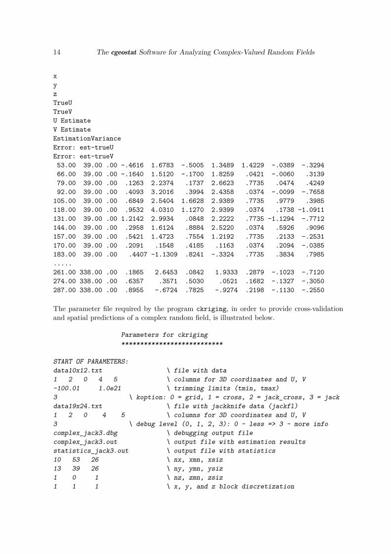
14 The cgeostat Software for Analyzing Complex-Valued Random Fields
xyzTrueUTrueVU EstimateV EstimateEstimationVarianceError: est-trueUError: est-trueV53.00 39.00 .00 -.4616 1.6783 -.5005 1.3489 1.4229 -.0389 -.329466.00 39.00 .00 -.1640 1.5120 -.1700 1.8259 .0421 -.0060 .313979.00 39.00 .00 .1263 2.2374 .1737 2.6623 .7735 .0474 .424992.00 39.00 .00 .4093 3.2016 .3994 2.4358 .0374 -.0099 -.7658
105.00 39.00 .00 .6849 2.5404 1.6628 2.9389 .7735 .9779 .3985118.00 39.00 .00 .9532 4.0310 1.1270 2.9399 .0374 .1738 -1.0911131.00 39.00 .00 1.2142 2.9934 .0848 2.2222 .7735 -1.1294 -.7712144.00 39.00 .00 .2958 1.6124 .8884 2.5220 .0374 .5926 .9096157.00 39.00 .00 .5421 1.4723 .7554 1.2192 .7735 .2133 -.2531170.00 39.00 .00 .2091 .1548 .4185 .1163 .0374 .2094 -.0385183.00 39.00 .00 .4407 -1.1309 .8241 -.3324 .7735 .3834 .7985.....261.00 338.00 .00 .1865 2.6453 .0842 1.9333 .2879 -.1023 -.7120274.00 338.00 .00 .6357 .3571 .5030 .0521 .1682 -.1327 -.3050287.00 338.00 .00 .8955 -.6724 .7825 -.9274 .2198 -.1130 -.2550
The parameter file required by the program ckriging, in order to provide cross-validationand spatial predictions of a complex random field, is illustrated below.
Parameters for ckriging***************************
START OF PARAMETERS:data10x12.txt \ file with data1 2 0 4 5 \ columns for 3D coordinates and U, V-100.01 1.0e21 \ trimming limits (tmin, tmax)3 \ koption: 0 = grid, 1 = cross, 2 = jack_cross, 3 = jackdata19x24.txt \ file with jackknife data (jackfl)1 2 0 4 5 \ columns for 3D coordinates and U, V3 \ debug level (0, 1, 2, 3): 0 - less => 3 - more infocomplex_jack3.dbg \ debugging output filecomplex_jack3.out \ output file with estimation resultsstatistics_jack3.out \ output file with statistics10 53 26 \ nx, xmn, xsiz13 39 26 \ ny, ymn, ysiz1 0 1 \ nz, zmn, zsiz1 1 1 \ x, y, and z block discretization

Journal of Statistical Software 15
3 8 \ #_min points, #_max points200.0 100.0 0.0 \ maximum search radii45.0 0.0 0.0 \ angles for search ellipsoid1 \ kriging type (0 = SK, 1 = OK)0.00 0.00 \ mean value(i), i = 1, 2 (nvar = 2)1 \ model for real part (= 1), imag part (= 2)1 0.0 -0.002596 0.001863 0.0 \ nst, c0, c1, c2, c33 21.5 45.0 0.0 0.0 \ it, cc, ang1, ang2, ang3
294.000 105.000 0.0 \ a_hmax, a_hmin, a_vert
Note that some parameters are clearly explained through the brief documentation reportedon the right side of the parameter file; on the other hand, some specific parameters, requiredby the program ckriging, are described in order of appearance in the following list:
• the kriging option: koption = 0 for complex kriging for a grid of points or blocks,koption = 1 for cross-validation with the data in datafl, koption = 2 or koption= 3 for jackknife with the data indicated in the jackknife file. If some data locationscoincide with some points in the jackknife file, then the option 2 of jackknife allowsthe coincident data to be removed one at a time and estimated from the remainingneighboring data as in cross-validation, while the option 3 of jackknife allows the coin-cident data to be included in the searching neighborhood (this option produces exactestimates);
• the name of the output file with the statistics regarding the available data and theestimated data;
• in the subsequent 3 lines, the definition of the grid in an ad-hoc coordinate system, whichis necessary for grid predictions (koption = 0); this is done in terms of the coordinatesat the center of the first node/block (xmn, ymn, zmn), the number of grid nodes/blocks(nx, ny, nz) and the size/spacing of the nodes/block (xsiz, ysiz, zsiz). Moredetails are given in the GSLib manual (Deutsch and Journel 1998);
• in the last 6 lines, the kriging type and the complex covariance model:
– the kriging type is set to 0 if simple kriging is performed; it is set to 1 if ordinarykriging is performed;
– in case of simple kriging, the known mean values for the two components must bedefined;
– the specifications of the complex covariance model in (4) can be provided for thereal part or alternatively for the complex part, since given the translating vector c,the complex part can be defined starting from the real part and vice versa; hence,the indicator is set to 1 if the specifications are given for the real part, while it isset to 2 if the specifications are given for the imaginary part;
– the parameter nst corresponds to the number of structures of C, used in (4);– the parameter c0 corresponds to the nugget effect;– the parameters c1, c2 and c3 represent the components of the translating vector c;– the parameter it corresponds to the model type of each structure (Table 1);

16 The cgeostat Software for Analyzing Complex-Valued Random Fields
– the parameter cc corresponds to the contribution of each structure of C;– the parameters ang1, ang2, ang3 correspond to the spatial angles and a_hmax,
a_hmin, a_vert correspond to the ranges or scales of variability of each structureof C.
In Table 1, the integer codes that can be used to specify the covariance models for the Cin (4) are provided. It is worth highlighting that the admissible complex covariance models,generated through Equation 4, have been implemented in the subroutine ccov3 which is calledby the program ckriging. Note that the same subroutine ccov3 is also called by the programccovamodel described in Section 3.4.
Run ckriging
If the parameter file has been suitably filled, then the user can run the program ckriging andtype the name of the prepared parameter file. The parameters set in the ad-hoc file are readand simultaneously displayed on the screen, then the input data files are read and saved in atemporary array, and some basic statistics are computed, as shown in the following template:
Variable 1 in data file: 4Number = 120.000000Average = 3.023375E-01Std. deviation = 1.861279Std. error = 1.699108E-01Minimum value = -3.611300Maximum value = 5.073600
Variable 2 in data file: 5Number = 120.000000Average = -4.459241E-02Std. deviation = 4.246270Std. error = 3.876297E-01Minimum value = -10.209100Maximum value = 7.186400
Variable 1 in jackknife file: 4Number = 456.000000Average = 1.856544E-01Std. deviation = 1.903301Std. error = 8.913024E-02Minimum value = -3.630000Maximum value = 6.635800
Variable 2 in jackknife file: 5Number = 456.000000Average = -9.362296E-03Std. deviation = 4.281832Std. error = 2.005152E-01Minimum value = -10.209100Maximum value = 8.978900
As soon as the program starts the kriging procedure, the note Working on the complex

Journal of Statistical Software 17
kriging is shown; moreover, a report on the working progress from time to time is alsoprovided on the screen, as given below:
Working on the complex krigingcurrently on estimate 12currently on estimate 24currently on estimate 36....currently on estimate 456
At the end, some descriptive statistics on the estimates of the two components are shown onthe screen and written to the debug file, then a closing message on the screen announces thatthe program has terminated, as shown in the following output template.
DESCRIPTIVE STATISTICS for est. values of U and V
Variable UEstimated 456 total blocksAverage = 2.409850E-01Std. deviation = 1.856171Std. error = 8.692319E-02Minimum value = -3.773563Maximum value = 5.201846
Variable VEstimated 456 total blocksAverage = 4.879891E-02Std. deviation = 4.252596Std. error = 1.991460E-01Minimum value = -10.384210Maximum value = 10.254780
TESTING HYPOTHESIS ON DIFFERENCE BETWEEN MEANS
P-value (H0: True mean_U = Est mean_U) = .6588P-value (H0: True mean_V = Est mean_V) = .8716
STATISTICS on the errors: True vs Est.
MAE for U = .4186RMSE for U = .6595
MAE for V = .6260RMSE for V = 1.0926
CKRIGING Version: 1.000 Finished
Stop - Program terminated.

18 The cgeostat Software for Analyzing Complex-Valued Random Fields
The output estimates and some statistics regarding available data and estimated data aresaved in two separate text files whose extensions (usually .out and .txt respectively) aredefined in the parameter file.As specified at the beginning, when the program ckriging is run, some error messages mightappear. In particular, for this specific program, some alerts may be issued
• to point out if the kriging option or the kriging type are not valid;
• to detect if the indicated model type of a basic structure does not exist (it is not one ofthe models in Table 1).
4. An application on complex dataIn the following case study, a vectorial data set with two components is interpreted as a finiterealization of a complex-valued random field W , with components U and V (or modulus anddirection in a polar system), and is analyzed by using the software cgeostat. A directory,called replication_materials, contains the executable files, the parameter files, the inputand output files used for the case study of this article.
4.1. Data set
The whole data set of the spatial vectorial values (data19x24.txt) refers to 456 locationsregularly distributed over a grid (19 × 24). However, a grid of (10 × 12) is selected and thecorresponding vectorial data (data10x12.txt) is used for structural analysis; the remainingdata is considered for comparison purposes in jackknife prediction.The vectorial representation of the available complex data over the (19 × 24) grid is pro-duced by applying the program clocmap with the parameter file clocmap19x24.par given inSection 3.1. On the other hand, the location map for the selected complex data is similarlyobtained by applying the program clocmap with the parameter file clocmap10x12.par givenbelow.
Parameters for CLOCMAP***********************
START OF PARAMETERS:data10x12.txt \ file with data1 2 0 4 5 0 \ columns for coords X, Y, Z & vars U, V, E-9990. 1.0e21 \ trimming limits for U-9990. 1.0e21 \ trimming limits for V-9990. 1.0e21 \ trimming limits for E0 \ option overlay: 0 = no, 1 = yesXXXX.txt \ file with conditioning data1 2 0 4 5 \ columns for coords X, Y, Z & vars U, V1 \ color code for conditioning data U, Vclocmap10x12.ps \ file for postscript output50.0 290. \ xmn, xmx35.0 340. \ ymn, ymx

Journal of Statistical Software 19
Figure 1: Location map of the available data set over a grid of a) (19× 24), b) (10× 12).
0.0 \ z selection8 \ color code for vector U, V0 \ 0 = arithmetic, 1 = log10 scaling(|u|>1, |v|>1)0.01 12.0 3 10 \ modulus scale & size: dmin, dmax, smin, smax0 \ 0 = no labels, 1 = label each location8 \ color code for variable E1 \ transform var.E: 0 = none, 1 = sqrt, 2 = log100.5 \ label size of var.E: 0.1 = sml, 1 = reg, 10 = bigLocation map of complex data \ title
The output files are shown in Figure 1.In the following, the complex covariance function is estimated and fitted, then complex pre-dictions, based on the selected complex covariance model, are computed over (19 × 24) gridnodes by using complex kriging implemented in the program ckriging.
4.2. Structural analysis and modeling
Given the class of models in (4), a suitable complex covariance function for the data understudy is found through
• the estimation of the covariance functions for components U and V of the complex ran-dom field W , denoted as CU and CV , and the corresponding cross-covariance functionsCUV and CVU for different lags and directions of the spatial domain;
• the estimation of the components, CRe and CIm , of the complex covariance functiongiven in (2), by computing the sum of the sample direct covariances CU and CV andthe difference of the sample cross-covariances CVU and CUV for relevant directions, andfitting of the parameter vector c;
• selection of an appropriate anisotropic covariance model C(·;θ) with parameter vector
20 The cgeostat Software for Analyzing Complex-Valued Random Fields
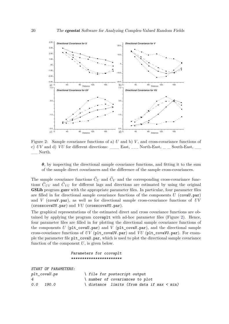
Figure 2: Sample covariance functions of a) U and b) V , and cross-covariance functions ofc) UV and d) VU for different directions: ___ East, _ _ _ North-East, _ _ South-East, ____ North.
θ, by inspecting the directional sample covariance functions, and fitting it to the sumof the sample direct covariances and the difference of the sample cross-covariances.
The sample covariance functions CU and CV and the corresponding cross-covariance func-tions CUV and CVU for different lags and directions are estimated by using the originalGSLib program gamv with the appropriate parameter files. In particular, four parameter filesare filled in for directional sample covariance functions of the components U (covaU.par)and V (covaV.par), as well as for directional sample cross-covariance functions of UV(crosscovaUV.par) and VU (crosscovaVU.par).The graphical representations of the estimated direct and cross covariance functions are ob-tained by applying the program ccovaplt with ad-hoc parameter files (Figure 2). Hence,four parameter files are filled in for plotting the directional sample covariance functions ofthe components U (plt_covaU.par) and V (plt_covaV.par), and the directional samplecross-covariance functions of UV (plt_covaUV.par) and VU (plt_covaVU.par). For exam-ple the parameter file plt_covaU.par, which is used to plot the directional sample covariancefunction of the component U , is given below.
Parameters for ccovaplt***********************
START OF PARAMETERS:plt_covaU.ps \ file for postscript output4 \ number of covariances to plot0.0 190.0 \ distance limits (from data if max < min)

Journal of Statistical Software 21
-3.0 5.0 \ covariance limits (from data if max < min)Directional Cov for U \ title for covariance function1 \ comp. on data to plot: none = 1, sum = 2, dif = 3covaU.txt \ 1 file with covariance dataXXX.txt \ 1 file with covariance data (only for type = 2, 3)1 0 1 1 8 \ covariance#, dash#(1-10), pts(1-0), line(1-0), colr1 \ comp. on data to plot: none = 1, sum = 2, dif = 3covaU.txt \ 1 file with covariance dataXXX.txt \ 1 file with covariance data (only for type = 2, 3)2 0 1 1 1 \ covariance#, dash#(1-10), pts(1-0), line(1-0), colr1 \ comp. on data to plot: none = 1, sum = 2, dif = 3covaU.txt \ 1 file with covariance dataXXX.txt \ 1 file with covariance data (only for type = 2, 3)3 0 1 1 2 \ covariance#, dash#(1-10), pts(1-0), line(1-0), colr1 \ comp. on data to plot: none = 1, sum = 2, dif = 3covaU.txt \ 1 file with covariance dataXXX.txt \ 1 file with covariance data (only for type = 2, 3)4 0 1 1 3 \ covariance#, dash#(1-10), pts(1-0), line(1-0), colr
In this case, the input files for the program ccovaplt correspond to the output files of theprogram gamv. The reader can find the other parameter files in the supplementary materialin directory replication_materials together with the case study results.Then the real and imaginary components of the complex covariance are estimated and mod-eled. In particular, given the class (4) of complex covariance models, the least squares tech-nique is first used for c1 and c2 estimation. The program cfitting with the parameter filegiven in Section 3.2, provides the least squares estimates for c1 and c2. Then the followingcomplex covariance model is fitted:
C(h; c,θ) = cos(h · c)C(h;θ) + i sin(h · c)C(h;θ), (8)
where C(h), with C(0) = 21.5, is a Gaussian covariance model with geometric anisotro-py, whose direction of maximum continuity is 45◦ with maximum range equal to 98 (cor-responding to an effective range of 294) and minimum range in the perpendicular direc-tion equal to 35 (corresponding to an effective range of 105), that is θ = (21.5, 294, 105),c = (−0.0025962, 0.0018629, 0.0). Note that the geometric characteristics of C(h) are fixedthrough visual inspection of the empirical direct and cross covariance functions. In particular,the real and imaginary parts of the complex covariance model are given below:
CRe(hx, hy; 45o) = 21.5 cos(−0.0025962hx + 0.0018629hy) exp[−(h/98)2],CRe(hx, hy; 135o) = 21.5 cos(−0.0025962hx + 0.0018629hy) exp(−(h/35)2),CIm(hx, hy; 45o) = 21.5 sin(−0.0025962hx + 0.0018629hy) exp(−(h/98)2),CIm(hx, hy; 135o) = 21.5 sin(−0.0025962hx + 0.0018629hy) exp(−(h/35)2),
where h =√h2x + h2
y.The program ccovamodel is applied to compute the real and imaginary parts of the com-plex covariance model. The parameter file used to produce the real component is given inSection 3.4, while the parameter file used to determine the imaginary part is illustrated below.

22 The cgeostat Software for Analyzing Complex-Valued Random Fields
Parameters for ccovamodel*************************
START OF PARAMETERS:ccovamodel_im.var \ file for covariance output2 \ real part = 1, imaginary part = 24 20 \ number of directions and lags90.0 0.0 4.5 \ azm, dip, lag distance45.0 0.0 8.5 \ azm, dip, lag distance
135.0 0.0 4.5 \ azm, dip, lag distance0.0 0.0 4.5 \ azm, dip, lag distance
1 0.0 -0.0025962 0.0018629 0.0 \ nst, nugget effect, c1, c2, c37 21.5 45.0 0.0 0.0 \ it, cc, ang1, ang2, ang3
294.000 105.000 0.0 \ a_hmax, a_hmin, a_vert
Both parameter files are filled in for computing the covariance model along 4 directions and20 lags. Note that the model specifications fixed in these parameter files are also used forcomplex kriging (see Section 4.3). As specified before, the output of this program containsalternatively the real component or the imaginary part of the complex covariance model (4)in accordance with the specification given at the second line of the parameter file, which is setequal to 1 for the real part computation, or equal to 2 for the imaginary part computation.The graphical representations of the sample directional components of the complex covariancefunction and the corresponding model are obtained by using the program ccovaplt. Fourparameter files are appropriately filled in, one for each direction. For example, the parame-ter file plt_ccova_SE.par is illustrated in Section 3.2 and it is prepared so that the sampledirectional components (real and imaginary) of the complex covariance function and the cor-responding model along the direction South-East are plotted. Note that, for a fixed direction,the sample real component is obtained by summing, lag by lag, the sample direct covariancefunctions for U and V , while the sample imaginary component is obtained by applying thedifference, lag by lag, of the sample cross-covariance function for VU with respect to the onefor UV . This reflects the theoretical equations given in (3). The reader can find the otherthree parameter files in the attached directory with the case study results. Figure 3 shows thereal and imaginary parts of the sample complex covariance function and the correspondingmodels computed for different directions.In Section 4.3, cross-validation, grid predictions and jackknife predictions are computed byapplying the above model characterizations.
4.3. Complex validation and predictionThe program ckriging is used for both cross-validation and prediction purposes (by usingthe grid option or the jackknife options) with the parameter files appropriately filled in.First of all, the complex covariance model for the corresponding random field is cross-validatedon the basis of the available data at the 120 spatial points located over a grid (10× 12). Theparameter file ckriging_cross.par used for cross-validation is presented below.
Parameters for ckriging***************************

Journal of Statistical Software 23
Figure 3: Real part of the sample complex covariance function (•) and its model (___)with the corresponding imaginary part (•) and its model (__ __) for different directions:a) East, b) North-East, c) South-East, d) North.
START OF PARAMETERS:data10x12.txt \ file with data (datafl)1 2 0 4 5 \ columns for 3D coordinates + 2 components-100.01 1.0e21 \ trimming limits (tmin, tmax)1 \ koption: 0 = grid, 1 = cross, 2 = jack_cross, 3 = jackXXX.txt \ file with jackknife data (jackfl)0 0 0 0 0 \ columns for 3D coordinates + 2 components3 \ debug level (0, 1, 2, 3)complex_cross.dbg \ debugging output filecomplex_cross.out \ output filestatistics_cross.out \ file for statistics10 53 26 \ nx, xmn, xsiz13 39 26 \ ny, ymn, ysiz1 0 1 \ nz, zmn, zsiz
1 1 1 \ x, y, and z block discretization3 8 \ #_min points, #_max points200.0 100.0 0.0 \ maximum search radii45.0 0.0 0.0 \ angles for search ellipsoid
1 \ kriging type (0 = SK, 1 = OK)

24 The cgeostat Software for Analyzing Complex-Valued Random Fields
0.00 0.00 \ mean value(i), i = 1, 2 (nvar = 2)1 \ model for real part (= 1), imag part (= 2)1 0.0 -.0025962 0.001862 0.0 \ nst, c0, c1, c2, c33 21.5 45.0 0.0 0.0 \ it, cc, ang1, ang2, ang3
294.00 105.00 0.0 \ a_hmax, a_hmin, a_vert
Note that
• the complex kriging option is set equal to 1, in order to produce cross-validation;
• the parameters related to jackknife predictions (such as the file name and the columnsfor the coordinates and the components U and V in the jackknife file) do not have tobe specified in this case;
• the file names which contain the debugging data, the cross-validation results and thecorresponding statistics are set equal to complex_cross.dbg, complex_cross.out andstatistics_cross.out, respectively;
• regarding the grid specifications, they are useful in GSLib algorithms for defining localsearch neighborhoods apart from the selected kriging option. In this case, the coordi-nates at the first point are (53, 39, 0), the grid nodes are 10 along the East direction,13 along the North direction and 0 in the vertical direction (indicating that a 2D grid isdefined) and the spacing between the nodes are, respectively, 26, 26 and 1. The size ofthis search network is usually much larger than the final estimation or simulation gridnode spacing (Deutsch and Journel 1998);
• regarding block discretization, the value 1 results in point kriging being performed;
• the characteristics of the search neighborhood are such that the estimation is performedby using from 3 to 8 sample data which fall in the ellipsoid whose maximum axis, alongthe direction of maximum continuity (corresponding to 45◦ clockwise from the azimuthdirection) is 200, and the minimum axis is 100. These values are fixed taking intoaccount the ranges of the covariance model;
• regarding the complex covariance model, the parameters are such that the fitted model(8) is considered.
Tables 2 and 3 illustrate some descriptive and inferential statistics for the original data valuesand the estimates, which are computed and saved in the output file statistics_cross.out.They can be compared and used to assess the estimation procedure and indirectly the fittedcovariance function.Indeed, a statistical test is conducted in order to verify that the differences between the meansof the true values and the estimated ones for the components U and V are nil. The p valuesof the test-statistics are determined (Tables 2 and 3) indicating that the null hypothesis isretained. Hence, the complex covariance function can be considered appropriate for modelingthe spatial correlation of the analyzed vectorial components, as also confirmed by computingthe mean absolute error (MAE) and the root mean square error (RMSE) between the truevalues and the estimated ones for the two components (Tables 2 and 3).

Journal of Statistical Software 25
Cross-validation Component X Component Ystatistics True Est. True Est.
Num. of data 120 120 120 120Mean 0.302 0.251 −0.046 0.007
Std. dev. 1.861 1.967 4.264 4.139Std. err. 0.170 0.180 0.388 0.378
Minimum −3.611 −4.020 −10.209 −9.689Maximum 5.074 5.976 7.186 6.884
Mean difference testHypoth. difference 0 0
p value 0.8361 0.9245MAE 1.0228 0.9781
RMSE 1.4027 1.3309
Table 2: Some statistics on cross-validation estimations.
Jackknife Component X Component Ystatistics True Est. Est. True Est. Est.
(op. 2) (op. 3) (op. 2) (op. 3)Num. of data 456 456 456 456 456 456
Mean 0.212 0.236 0.250 0.045 0.055 0.042Std. dev. 1.908 1.878 1.850 4.262 4.231 4.259Std. err. 0.089 0.088 0.087 0.200 0.198 0.199
Minimum −3.630 −4.020 −3.611 −10.209 −10.448 −10.448Maximum 6.636 5.976 5.246 8.979 9.200 9.200
Mean difference testHypoth. difference 0 0 0 0
p value 0.8465 0.7615 0.9709 0.9908MAE 0.6525 0.3834 0.8585 0.6011
RMSE 0.9422 0.6082 1.2578 1.0563
Table 3: Some statistics on jackknife estimations with the kriging options 2 and 3.
After cross-validation, the new program ckriging is applied to predict the variable understudy through complex ordinary kriging.First of all, the grid option is considered; in particular, the above discussed covariance modelis used for the estimation of the two components U and V over a grid (19×24). The parameterfile used for the grid prediction is given below.
Parameters for ckriging***************************
START OF PARAMETERS:data10x12.txt \ file with data (datafl)1 2 0 4 5 \ columns for 3D coordinates + 2 components-100.01 1.0e21 \ trimming limits (tmin, tmax)0 \ koption: 0 = grid, 1 = cross, 2 = jack_cross, 3 = jack

26 The cgeostat Software for Analyzing Complex-Valued Random Fields
XXX.txt \ file with jackknife data (jackfl)0 0 0 0 0 \ columns for 3D coordinates + 2 components3 \ debug level (0, 1, 2, 3)complex_grid.dbg \ debugging output filecomplex_grid.out \ output filestatistics_grid.out \ file for statistics19 53 13 \ nx, xmn, xsiz24 39 13 \ ny, ymn, ysiz1 0 1 \ nz, zmn, zsiz
1 1 1 \ x, y, and z block discretization3 8 \ #_min points, #_max points200.0 100.0 0.0 \ maximum search radii45.0 0.0 0.0 \ angles for search ellipsoid
1 \ kriging type (0 = SK, 1 = OK)0.00 0.00 \ mean value(i), i = 1, 2 (nvar = 2)1 \ model for real part (= 1), imag part (= 2)1 0.0 -.0025962 0.001862 0.0 \ nst, c0, c1, c2, c33 21.5 45.0 0.0 0.0 \ it, cc, ang1, ang2, ang3
294.00 105.00 0.0 \ a_hmax, a_hmin, a_vert
Successively, the entire data set (not used for structural analysis) is also considered for thejackknife options 2 and 3. The two parameter files used for jackknife predictions, which arenamed ckriging_jack2.par and ckriging_jack3.par, are equal to the previous one exceptfor the kriging option which is set equal to 2 for the former and 3 for the latter (the parameterfile is illustrated in Section 3.5).In Table 3, some descriptive and inferential statistics regarding the jackknife results, withboth options, are given. It is worth underlining that the estimation results over the grid(19×24) obtained through the grid option (koption = 0) are equal to the ones obtained withthe jackknife option 3 (koption = 3) over the same grid (19×24), except that this last optionprovides the comparisons with the true values.The statistical test on the mean difference of the two components confirms that the null hy-pothesis of zero means can be accepted with low margin of uncertainty, in terms of p values.Moreover, note that both MAE and RMSE highlight the capability of the algorithm to re-produce the vectorial random field. Thus, the jackknife results show that the method canrecover the unknown truth when every part of the model is correctly specified.Figure 4 shows the prediction map of the complex-valued random field for the study area,together with the error standard deviation (square root of the error variance), and the condi-tioning data (available data over the grid (10 × 12)), marked with red arrows. This locationmap is obtained by using the program clocmap with the parameter file clocmap_jack.pargiven below.
Parameters for CLOCMAP***********************
START OF PARAMETERS:complex_jack3.out \ file with data1 2 0 6 7 8 \ columns for coords X, Y, Z & vars U, V, E-9990. 1.0e21 \ trimming limits for U

Journal of Statistical Software 27
50. 100. 150. 200. 250.
35.
135.
235.
335.
Modulus
12.000
.01000
Error std. dev.
up to .1703
up to 1.031
Figure 4: Location map of the predicted values of the complex random field W , throughcomplex kriging (→), and the conditioning data over a grid (10 × 12) (→).
-9990. 1.0e21 \ trimming limits for V-9990. 1.0e21 \ trimming limits for E0 \ option overlay: 0 = no, 1 = yesdata10x12.txt \ file with conditioning data1 2 0 4 5 \ columns for coords X, Y, Z & vars U, V1 \ color code for conditioning data U, Vclocmap_jack.ps \ file for postscript output50.0 290. \ xmn, xmx35.0 340. \ ymn, ymx0.0 \ z selection8 \ color code for vector U, V0 \ 0 = arithmetic, 1 = log10 scaling(|u|>1, |v|>1)0.01 12.0 3 10 \ modulus scale & size: dmin, dmax, smin, smax0 \ 0 = no labels, 1 = label each location8 \ color code for variable E1 \ transform var.E: 0 = none, 1 = sqrt, 2 = log100.5 \ label size of var.E: 0.1 = sml, 1 = reg, 10 = big
\ title
5. SummaryIn this paper, some dedicated Fortran programs for geostatistical analysis of a finite realizationof a complex-valued random field are presented. Complex kriging and some other programs,for representing complex data, computing and plotting components of a sample complexcovariance function, computing and plotting components of a complex covariance model,
28 The cgeostat Software for Analyzing Complex-Valued Random Fields
have been implemented and an application on vectorial data with two components has beenproposed. In particular, these routines are customized programs generated, on the basis ofthe GSLib library (specifically the version GSLIB77), for analyzing complex-valued randomvariables on a spatial domain Rd (d ≤ 3).The new GSLib programs ckriging, clocmap, ccovaplt, cfitting and ccovamodel, providesome computational solutions, which had not been implemented in the GSLib library before.In particular, the program ckriging faces the problem of estimating a complex-valued randomfield. Differently from the original kriging program KT3D, the following computational aspectshave been considered in the program ckriging:
• complex kriging systems, given in (6) and (7), have been implemented;
• the program COVA3, which belongs to the GSLib library, has been modified in orderto include the admissible complex covariance model, defined in expression (4). Thismodified program has been renamed ccov3 and it has been included in the main programckriging.for. In this way, it has not been necessary to modify the GSLib library;
• simultaneous estimations of the two variables, which are the two components of thecomplex-valued random field, and the associated error variance are computed;
• another kriging option for jackknife estimation has been included: the option 3 ofjackknife allows the coincident data (the ones which coincides with the data locations)to be included in the searching neighborhood. This produces exact estimates associatedwith the jackknife points which are coincident with that data locations;
• at the end, some descriptive statistics on the estimates of the two components are shownon the screen and written in a text file; moreover the mean absolute errors and the meansquare errors for both components are computed, shown on the screen and written onthe same text file.
Similarly, the other programs provide innovative tools for analyzing and representing complexvariables and their correlation structure.In the future, various complex covariance models and different forms of predictors for com-plex variables can be considered. It is worth highlighting that the implementation in theR environment and the extension to a spatio-temporal context might be also interesting aswell as the idea of understanding if the complex-valued random fields models can adhere tosolutions of particular partial differential equations should be investigated in the future.
AcknowledgmentsI would like to really thank the editors and the reviewers for the interest demonstrated andthe precious suggestions which have contributed to improve the paper.
References
Austenfeld M, Beyschlag W (2012). “A Graphical User Interface for R in a Rich ClientPlatform for Ecological Modeling.” Journal of Statistical Software, 49(4), 1–19. doi:10.18637/jss.v049.i04.

Journal of Statistical Software 29
Barry R (1996). “A Diagnostic to Assess the Fit of a Variogram Model to Spatial Data.”Journal of Statistical Software, 1(1), 1–11. doi:10.18637/jss.v001.i01.
Chilés JP, Delfiner P (1999). Geostatistics: Modeling Spatial Uncertainty. John Wiley &Sons, New York.
Cressie N, Huang HC (1999). “Classes of Nonseparable, Spatio-Temporal Stationary Co-variance Functions.” Journal of the American Statistical Association, 94(448), 1330–1340.doi:10.2307/2669946.
De Cesare L, Myers DE, Posa D (2002). “Fortran Programs for Space-Time Modeling.” Com-puters & Geosciences, 28(2), 205–212. doi:10.1016/s0098-3004(01)00040-1.
De Iaco S, Maggio M, Palma M, Posa D (2012). “Advances in Spatio-Temporal Modelingand Prediction for Environmental Risk Assessment.” In B Haryanto (ed.), Air Pollution:A Comprehensive Perspective, chapter 14, pp. 365–390. InTech. doi:10.5772/51227.
De Iaco S, Myers DE, Palma M, Posa D (2010). “Fortran Programs for Space-Time Mul-tivariate Modeling and Prediction.” Computers & Geosciences, 36(5), 636–646. doi:10.1016/j.cageo.2009.10.004.
De Iaco S, Palma M, Posa D (2003). “Covariance Functions and Models for Complex-ValuedRandom Fields.” Stochastic Environmental Research and Risk Assessment, 17(3), 145–156.doi:10.1007/s00477-003-0129-5.
De Iaco S, Posa D (2012). “Predicting Spatio-Temporal Random Fields: Some ComputationalAspects.” Computers & Geosciences, 41(4), 12–24. doi:10.1016/j.cageo.2011.11.014.
De Iaco S, Posa D, Palma M (2013). “Complex-Valued Random Fields for Vectorial Data:Estimating and Modeling Aspects.” Mathematical Geosciences, 45(5), 557–573. doi:10.1007/s11004-013-9468-z.
Deutsch CV, Journel AG (1998). GSLib: Geostatistical Software Library and User’s Guide.Applied Geostatistics Series, 2nd edition. Oxford University Press, New York.
Diggle PJ, Ribeiro Jr PJ (2007). Model Based Geostatistics. Springer-Verlag, New York.
Dutter R (1996). Analysis of Spatial Data Using GEOSAN: A Program System for Geosta-tistical Analysis. University of Technology, Vienna, Austria. Handbook.
Englund E (1991). Geo-EAS 1.2.1: Geostatistical Environmental Assessment Software. User’sGuide. Environmental Monitoring Systems Laboratory, Office of Research and Develop-ment, U.S. Environmental Protection Agency, Las Vegas, Nevada.
Gabriel E, Rowlingson B, Diggle PJ (2013). “stpp: An R Package for Plotting, Simulatingand Analysing Spatio-Temporal Point Patterns.” Journal of Statistical Software, 53(2),1–29. doi:10.18637/jss.v053.i02.
Geovariances (2015). ISATIS Software. Geovariances, Avon, France.
Haslett J, Raftery AE (1989). “Space-Time Modelling with Long-Memory Dependence: As-sessing Ireland’s Wind-Power Resource.” Applied Statistics, 38(1), 1–50. doi:10.2307/2347679.
30 The cgeostat Software for Analyzing Complex-Valued Random Fields
Lajaunie C, Béjaoui R (1991). Sur le krigeage des functions complexes. Note N-23/91/G.Centre de Geostatistique, Ecole des Mines de Paris, Fontainebleau.
Laurent T, Ruiz-Gazen A, Thomas-Agnan C (2012). “GeoXp: An R Package for ExploratorySpatial Data Analysis.” Journal of Statistical Software, 47(2), 1–23. doi:10.18637/jss.v047.i02.
Melo C, Santacruz A, Melo O (2015). geospt: An R Package for Spatial Statistics. R packageversion 1.0-2, URL https://CRAN.R-project.org/package=geospt.
Pebesma EJ (2004). “Multivariable Geostatistics in S: The gstat Package.” Computers &Geosciences, 30(7), 683–691. doi:10.1016/j.cageo.2004.03.012.
Pebesma EJ (2012). “spacetime: Spatio-Temporal Data in R.” Journal of Statistical Software,51(7), 1–30. doi:10.18637/jss.v051.i07.
Pebesma EJ, Bivand RS (2005). “Classes and Methods for Spatial Data in R.” R News, 5(2),9–13.
Pebesma EJ, Wesseling CG (1998). “gstat: A Program for Geostatistical Modelling,Prediction and Simulation.” Computers & Geosciences, 24(1), 17–31. doi:10.1016/s0098-3004(97)00082-4.
R Core Team (2017). R: A Language and Environment for Statistical Computing. R Founda-tion for Statistical Computing, Vienna, Austria. URL https://www.R-project.org/.
Remy N, Boucher A, Wu J (2009). Applied Geostatistics with SGeMS: A User’s Guide.Cambridge University Press, New York.
Renard D, Desassis N, Beucher H, Ors F, Laporte F (2014). “RGeostats: The GeostatisticalPackage.” Mines Paris Tech.
Ribeiro Jr PJ, Diggle PJ (2001). “geoR: A Package for Geostatistical Analysis.” R News,1(2), 15–18.
Schlather M, Malinowski A, Menck PJ, Oesting M, Strokorb K (2015). “Analysis, Simulationand Prediction of Multivariate Random Fields with Package RandomFields.” Journal ofStatistical Software, 63(8), 1–25. doi:10.18637/jss.v063.i08.
Statios LLC (2001). WinGSLIB: Geostatistical Software Library, version 1.4 for Windows.
Wackernagel H (2003). Multivariate Geostatistics: An Introduction with Applications.Springer-Verlag, Berlin.

Journal of Statistical Software 31
A. Data files and parameter files
This appendix provides some GSLib standards in terms of the format of the data files andthe parameter files required by the executable files.There is no choice for the user to specify explicitly the input format (usually Geo-EAS format),however the accessibility of the source code allows this to be changed. Missing data arecodified with large negative or positive numbers (e.g., −9999, or 9999, or −1.0e21 or 1.0e21).It is important to highlight that the programs read numerical values and not alphanumericstrings. In the presence of alphanumeric variables, these can be transformed to integers oralternatively the source code can be modified.All the variables, options and names of input/output files are contained in a parameter file.In the parameter files, the parameter values can be appropriately stated on the left side, whilea brief documentation of the parameters are reported on the right side. The user can addas many lines of comments at the top of the parameter file as desired, but formatted inputstarts immediately after the string “START”. Example of parameter files are included in thepaper. Each program requires its own parameter file, whose name is given by the user froma keyboard entry. Indeed, consistently to the GSLib standards, when one of the providedprograms of the cgeostat software is run, the following question appears:
Which parameter file do you want to use?
Then, the user has to type the name of the parameter file, previously filled, with its absolutepath or relative to the current working directory. If no file name is typed, then the programwould look for the parameter file which has the same name as the program and the extension.par (for example, the program ckriging would automatically look for ckriging.par). Ifthe parameter file is not found a blank parameter file is created and the program stops.Otherwise if the parameter file is found, the parameter values are read from the parameterfile and are simultaneously displayed on the screen.A closing message on the screen announces that the program has terminated, as shown in thefollowing output template
Stop - Program terminated.
The input and output files are saved in the folder the users are working in, unless a differentpath is specified in the parameter file.When a serious error is encountered, an error alert is displayed on the screen and the programis stopped. Sometimes less serious problems or inconsistencies cause a warning to be displayedon the screen or in a debugging file, and the program will continue. In particular, when aprogram is run, some error messages might appear in order, for example, to acknowledge ifthe input files are missing or to indicate if the parameter file does not respect the prefixedstandard.However, it is possible to make a mistake that has not been foreseen. In that case, check theinput and compare it to the data. If you cannot solve the problem, send the parameter fileand data file to [email protected].

32 The cgeostat Software for Analyzing Complex-Valued Random Fields
B. Dependencies of the programs on the rest of the GSLibAs already specified, the new GSLib routines call some programs which belong to the GSLiblibrary. In particular, the programs in the library which are called by the new program, arelinked to the main program through the file gslib.lib, located in the subdirectory gslibunder the directory DOS (for Windows binary users), or through the file libgs.a, located inthe subdirectory gslib under the directories LIN and Mac (for Mac or Linux users).Moreover, in a preliminary step of structural analysis of a complex random field, direct andcross-covariance functions have to be estimated. As specified in the case study, this can bedone by using the original GSLib routine gamv.
Affiliation:Sandra De IacoDepartment of Management, Economics, Mathematics and StatisticsUniversità del Salento73100 Lecce, ItalyE-mail: [email protected]: http://www.economia.unisalento.it/personale_docente
Journal of Statistical Software http://www.jstatsoft.org/published by the Foundation for Open Access Statistics http://www.foastat.org/
July 2017, Volume 79, Issue 5 Submitted: 2014-01-13doi:10.18637/jss.v079.i05 Accepted: 2016-07-10