November 2009

The Carry Trade and Fundamentals:

Nothing to Fear But FEER Itself∗

Abstract

The carry trade is the investment strategy of going long in high-yield target currencies and short in low-yield funding currencies. Recently, this naıve trade has seen very high returns for long periods, followedby large crash losses after large depreciations of the target currencies. Based on low Sharpe ratios andnegative skew, these trades could appear unattractive, even when diversified across many currencies. Butmore sophisticated conditional trading strategies exhibit more favorable payoffs. We apply novel (withineconomics) binary-outcome classification tests to show that our directional trading forecasts are informa-tive, and out-of-sample loss-function analysis to examine trading performance. The critical conditioningvariable, we argue, is the fundamental equilibrium exchange rate (FEER). Expected returns are lower,all else equal, when the target currency is overvalued. Like traders, researchers should incorporate thisinformation when evaluating trading strategies. When we do so, some questions are resolved: negativeskewness is purged, and market volatility (VIX) is uncorrelated with returns; other puzzles remain: themore sophisticated strategy has a very high Sharpe ratio, suggesting market inefficiency.

Oscar Jorda and Alan M. TaylorDepartment of EconomicsUniversity of CaliforniaDavis CA 95616e-mail (Jorda): ojorda@ucdavis.edue-mail (Taylor): amtaylor@ucdavis.eduKeywords: uncovered interest parity, efficient markets hypothesis, exchange rates.

JEL codes: C44, F31, F37, G14, G15, G17

∗Taylor has been supported by the Center for the Evolution of the Global Economy at UC Davis andJorda by DGCYT Grant (SEJ2007-63098-econ); part of this work was completed whilst Taylor was a Houblon-Norman/George Fellow at the Bank of England; all of this research support is gratefully acknowledged. We thankTravis Berge and Yanping Chong for excellent research assistance. We acknowledge helpful comments from VineerBhansali, Richard Meese, Michael Melvin, Stefan Nagel, Michael Sager, Mark Taylor, and seminar participants atThe Bank of England, Barclays Global Investors, London Business School, London School of Economics, the 3rdannual JIMF-SCCIE conference, the NBER IFM program meeting, and PIMCO. All errors are ours.

What is the fate of the efficient markets hypothesis (EMH)? Speaking to The Economist afterthe recent asset market turmoil, Richard Thaler has noted that the hypothesis always had twoparts. Part one, the “no-free-lunch part” and part two, the “price-is-right” part. He affirmed thatthe asset price bubble and bust have effectively demolished part two—and yet, by erasing manycumulative gains and exposing the weakness of many investment strategies, may have bolsteredsupport for part one, at least as a long-run proposition.1

In this paper, we re-examine the EMH using one of the most salient and well-trodden testinggrounds, the foreign exchange market and the ongoing debate over the carry trade that hasreignited once again. Once a relatively obscure corner of international finance, the naıve carrytrade (borrowing in low interest rate currencies and investing in high interest rate currencies,despite the exchange rate risk) has drawn increasing attention in recent years, within and beyondacademe, and especially as the volume of carry trade activity multiplied astronomically.

Inevitably, press attention has often focused on the personal angle. In 2007, The New YorkTimes reported on the disastrous losses suffered by the “FX Beauties” club and other Japaneseretail investors during an episode of yen appreciation; one highly-leveraged housewife lost herfamily’s entire life savings within a week.2 By the fall of 2008 attention was grabbed by an evenmore brutal squeeze on carry traders from bigger yen moves—e.g., up 60% against the AUD over 2months, and up 30% against GBP (including 10% moves against both in five hours on the morningof October 24). Money managers on the wrong side saw their funds blowing up, supporting theJune 2007 prediction of Jim O’Neill, chief global economist at Goldman Sachs, who had said ofthe carry trade that “there are going to be dead bodies around when this is over.”3

Economists have also been paying renewed attention to the carry trade, revisiting old questions:Are there returns to currency speculation? Are the returns predictable? Is there a failure of marketefficiency? We are still far from a consensus, but the present state of the literature, how it gotthere, and how it relates to the interpretations of the current market turmoil, can be summarizedin a just few moments, so to speak.4

The first point concerns the first moment of returns. There have been on average positivereturns to naıve carry trade strategies for long periods.5 Put another way, the standard findingof a “forward discount bias” in the short run means that exchange rate losses will not fully offset

1 “Efficiency and beyond,” The Economist, July 16th, 2009.2 Martin Fackler, “Japanese Housewives Sweat in Secret as Markets Reel,” New York Times, September 16,

2007.3 Ambrose Evans Pritchard. “Goldman Sachs Warns of ‘Dead Bodies’ after Market Turmoil,” Daily Telegraph,

June 3, 2007.4 For a full survey of foreign exchange market efficiency see Chapter 2 in Sarno and Taylor (2002), on which we

draw here.5 We prefer to focus on the period of unfettered arbitrage in the current era financial globalization—that is,

from the mid 1980s on, for major currencies. Staring in the 1960s the growth of the Eurodollar markets hadpermitted offshore currency arbitrage to develop. Given the increasingly porous nature of the Bretton Woods eracapital controls, and the tidal wave of financial flow building up, the dams started to leak, setting the stage forthe trilemma to bite in the crisis of the Bretton Woods regime in 1970–73. Floating would permit capital accountliberalization, but the process was fitful, and not until 1990s was the transition complete in Europe (Bakker andChapple 2002). Empirical evidence suggests significant barriers of 100bps or more even to riskless arbitrage in the1970s and even into the early 1980s (Frenkel and Levich 1975; Clinton 1988; Obstfeld and Taylor 2004). Takingthese frictions as evidence of imperfect capital mobility we prefer to exclude the 1970s and the early 1980s from ourempirical work. Other work, e.g. Burnside, Eichenbaum, Kleshchelski, and Rebelo (2008a,b) includes data back tothe the 1970s.

1

the interest differential gains of the naıve carry strategy.6 This finding is often misinterpreted asa failure of uncovered interest parity; but UIP is an ex-ante, not an ex-post, condition—and theevidence, albeit limited, shows that average ex-ante exchange rate expectations (e.g., from surveysof traders) are not so far out of line with interest differentials.7 Rather, expectations themselvesseem to be systematically wrong. In this view, ex-post profits appeared to be both predictable andprofitable, contradicting the risk-neutral efficient markets hypothesis. Indeed, our paper builds onthis tradition using both regression and trading-algorithm approaches.8 However, over periods ofa decade or two it is quite difficult to reject ex-post UIP, suggesting that interest arbitrage holdsin the long run, and that the possible profit opportunities are a matter of timing.9

The second point concerns the second moment of returns. If positive ex-ante returns are notarbitraged away, one way to rationalize them might be that they are simply too risky (volatile)to attract additional investors who might bid them away. This explanation has much in commonwith other finance puzzles, like the equity premium puzzle. The annual reward-to-variability ratioor Sharpe ratio of the S&P 500, roughly 0.4, can be taken as a benchmark level of risk adjustedreturn. But anecdotal evidence suggests that investors have little interest in strategies with annualSharpe ratios below 1, and that this hurdle applies to a currency strategy as much as any other.10

Historical data show that for all individual currency pairs, this hurdle has not been met usingnaıve carry trade strategies. Obviously, diversification in a portfolio across many currency pairscan improve performance, since returns on different currencies are not perfectly correlated. Buteven then, the data show that the hurdle of 1 is hard to beat in the long run for the G10 universeof currencies. Thus, the seemingly excess returns to the naıve carry strategy may be explicable,at least in part, as compensation for volatility.11,12

Finally, we turn to the third point of near consensus, on the third moment of returns. Naıve6 Seminal studies of the forward discount puzzle include Frankel (1980), Fama (1984), Froot and Thaler (1990),

and Bekaert and Hodrick (1993).7 Seminal works on survey expectations include Dominguez (1986) and Froot and Frankel (1987, 1989). For an

update see Chinn and Frankel (2002).8 A standard test of the predictability of returns (the “semi-strong” form of market efficiency) is to regress

returns on an ex ante information set. The seminal work is Hansen and Hodrick (1980). Other researchers deploysimple profitable trading rules as evidence of market inefficiency (Dooley and Shafer 1984; Levich and Thomas1993; Engel and Hamilton 1990).

9 Support for long-run UIP was found using long bonds by Fujii and Chinn (2000) and Alexius (2001), andusing short rates by Sinclair (2005).

10 Lyons (2001).11 It is an open question whether expanding the currency set to include minor currencies, exotics, and emerging

markets can add further diversification and so enhance the Sharpe ratio, or whether these benefits will be offsetby illiquidity, trading costs, and high correlations/skew. Burnside, Eichenbaum, Kleshchelski and Rebelo (2006)compute first, second, and third moments for individual currencies and portfolio-based strategies for major cur-rencies and some minor currencies. In major currencies the transaction costs associated with bid-ask spreads areusually small, although 5–10 bps per trade can add up if an entire portfolio is churned every month (i.e., 60–120bps annual). Burnside, Eichenbaum, and Rebelo (2007) explore emerging markets with adjustments for transactioncosts. Both studies conclude that there are profit opportunities net of such costs, but the Sharpe ratios are low.Moreover, Sager and Taylor (2008) argue that the Burnside et al. returns and Sharpe ratios may be overstated.Pursuing a different strategy, however, using information in the term structure, Sager and Taylor are able to attainSharpe ratios of 0.88 for a diversified basket of currencies in back testing.

12 In this paper we proceed in a risk-neutral framework, a widely-used benchmark, in contrast to the more recentand contentious use of consumption-based asset pricing models in the carry trade context. Lustig and Verdehlan(2007) claimed that the relatively low naıve carry trade returns may be explicable in a consumption-based modelwith reasonable parameters. Burnside (2007) challenged the usefulness of this approach. Returns to our systematictrading rules have very different moments, however, with mean returns twice as large as the typical naıve strategy,leaving a considerable premium to be explained in either framework.

2

carry trade returns are negatively skewed. The lower-tail risk means that trades are subjectto a risk of pronounced periodic crashes—what is often referred to as a peso problem. Such adescription applies to the aforementioned disaster events suffered by yen carry traders in 2007 and2008 (and their predecessors in 1998). However, many competing investments, like the S&P500, arealso negatively skewed, so the question is once more relative. And once again echoing the centrallimit theorem, this time for higher moments, while individual currency pairs may exhibit highskew, we know that diversification across currency pairs can be expected to drive down skewnessin a portfolio. But for naıve strategies some negative skew still remains under diversification, andit is then unclear whether excess returns are a puzzle, or required compensation for skew (and/orvolatility).13

Returning to Thaler’s summary of the EMH, the awful recent performance of naıve carry tradesfits with his perspective as applied to the FX market. But we will show that more sophisticatedFX trading strategies could, and did, avoid crashes, so the free lunch issue remains open to debate.Specifically, the contribution of our paper is as follows:

• We start from common ground and confirm all of the above findings for our data; naıve carrytrades are profitable but, even when diversified, they have low Sharpe ratios and negativeskew.14

• We show that an important explanatory variable has been omitted from influential priorstudies; the deviation from the fundamental equilibrium exchange rate (FEER) is an impor-tant predictor of exchange rates.

• Moreover, carry returns may be better explained in a nonlinear model, and our preferrednonlinear model draws together extant ideas from the UIP and PPP literature. The nonlinearmodel’s regimes weigh two signals, a “greed” factor (potential carry trade interest gains plusmomentum) and a “fear” factor (potential mean reversion to FEER).

• Inclusion of the FEER control variable improves not only the statistical performance ofthe model, it also enhances the financial performance of trading rules based on the model,and much more so than diversification alone. For simplicity and comparability we applythe model to equal-weight portfolio strategies among G10 currencies, which is the standardbacktesting laboratory. Trading on a long-short directional signal for each currency weachieve Sharpe ratios well in excess of 1 over long periods, and attain zero or even positiveskew.

• To support the claim that our directional forecasts beat a coin toss or rival strategies likenaıve carry, we do out-of-sample testing using innovative loss functions (Giacomini and

13 Brunnermeier, Nagel and Pedersen (2008) focus on the “rare event” of crash risk as an explanation for carrytrade profits. Burnside, Eichenbaum, Kleshchelski, and Rebelo (2008a) argue that peso problems cannot explaincarry trade profits, although in a different version of the same paper (2008b), they argue to the contrary.

14 Note that throughout this article we implicitly assume that the end investor dislikes negative skew, all elseequal. Of course, due to well known principal-agent problems arising from asymmetric compensation structures,asset managers may be quite happy to embrace large negative skew if they can obtain larger returns and associatedperformance fees in the short run before their fund blows up.

3

White 2006). We also employ (as far as we know, for the first time in economics) a set ofpowerful tools that have been widely used in other fields, such as medical statistics: thereceiver operating characteristic curve, or ROC curve, and its associated hypothesis tests.For applications in finance we apply an extension of the ROC curve, called ROC* (Jordaand Taylor 2009), which allows for directional predictions to be weighted by on returns, inthe spirit of gain-loss performance measures (Bernardo and Ledoit 2000).

• We also compare our approach to rival crash protection strategies. One suggestion is thatcarry trade skew is driven by market stress and liquidity events (Brunnermeier et al. 2008);but we find that VIX signals provide no additional explanatory or predictive power in ourpreferred forecasting framework. Another approach suggests that options provide a way tohedge downside risk (Burnside, Eichenbaum, Kleshchelski, and Rebelo, 2008ab); but thesestrategies are very costly to implement compared to our trading rule.

• Finally we perform out-of-sample tests and explore real-world trading strategies for the yearsup to and including the 2008 financial crisis, looking at our model performance and actualexchange traded funds. The naıve models and crude ETFs crashed horribly in 2008, wipingout years of gains. More sophisticated ETFs resembling our preferred model weathered thestorm remarkably well with barely any drawdown.

To conclude, we find that in the past, whilst naıve carry strategies may not have offeredadequate compensation for risk (volatility and skew), more sophisticated strategies that accountedfor long-run real exchange rate fundamentals could have easily surmounted that hurdle. Thisprovides support for currency strategies that augment carry and momentum signals with a valuesignal based on real fundamentals. Many sophisticated funds with limited access have pursuedsuch strategies in the past, but the recent arrival of simple, passive ETFs with these same featuresraises the question of how much “true alpha” active currency managers create. It also begs thequestion how long any such excess returns might persist before being arbitraged away.15

In addition to extending a growing econometric literature on the nature of carry trade dynam-ics, our paper also provides a touchstone for ongoing theoretical work that attempts to characterizethe form and extent of deviations from the efficient markets hypothesis. Our work is sympatheticto a well-established view that asset prices can deviate from their fundamental value for sometime, before a “snap back” occurs (Poterba and Summers 1986; Plantin and Shin 2007). Recenttheory has focused on what might permit the deviation, and what then triggers the snap. In FXmarkets, work in this vein includes models of noise traders, heterogeneous beliefs, rational inat-tention, liquidity constraints, herding, “behavioral” effects, and other factors that may serve tolimit arbitrage (e.g., Shleifer and Vishny 1997; Jeanne and Rose 2002; Baccheta and van Wincoop2006; Fisher 2006; Brunnermeier et al. 2008; Ilut 2008).

15 Pojarliev and Levich (2007, 2008) argue that active managers deliver less alpha than claimed, and that muchof their returns can be described as quasi-beta with respect to style factors like carry, momentum, and value thatare now captured in passive indices and funds.

4

1 Statistical Design

Our primary objectives are to investigate the dynamic links between the excess returns to carrytrade and deviations from FEER; to generate forecasts with which to construct out-of-sampleformal predictive evaluation; and hence to construct carry trade strategies whose out-of-samplereturns can be evaluated for profitability and risk.

The data for the analysis consists of a panel of nine countries (Australia, Canada, Germany,Japan, Norway, New Zealand, Sweden, Switzerland, and the United Kingdom) set against theU.S. over the period January 1986 to December, 2008, observed at a monthly frequency (i.e.,the “G10” sample).16 The variables in this data-set include the end-of-month nominal exchangerate expressed in U.S. dollars per foreign currency units and whose logarithm we denote as et;the one-month London interbank offered rates (LIBOR) denoted as it for the U.S. and i∗t for anyof the eight counterparty countries; and the consumer price index, whose logarithm is denotedas pt for the U.S. and p∗t otherwise. Data on exchange rates and the consumer price index areobtained from the IFS database whereas data on LIBOR are obtained from the British Banker’sAssociation (www.bba.org.uk) and Global Financial Data (globalfinacialdata.com).

The primary variable of interest to us can be thought of as momentum, denoted mt. Momentumrefers to the ex-post nominal excess returns of a carry trade, specifically approximated by

mt+1 = ∆et+1 + (i∗t − it). (1)

In the absence of barriers or limits to arbitrage, and assuming that the efficient markets hypothesis(EMH) holds, the ex-ante value of momentum should be zero, that is Etmt+1 = Et∆et+1 + (i∗t −it) = 0.

Momentum can also be expressed in terms of real excess returns as

mt+1 = ∆qt+1 + (r∗t − rt) (2)

where rt = it − πt+1 with πt+1 = ∆pt+1, and similarly for r∗t and π∗t+1; and qt+1 = q + et+1 +(p∗t+1 − pt+1) so that ∆qt+1 = ∆et+1 +

(π∗t+1 − πt+1

)and the equivalence between (1) and (2) is

readily apparent. Under the assumption of (weak) purchasing power parity, q is the mean FEERto which qt reverts, so qt − q is a stationary variable and hence a cointegrating vector. In a moregeneral setting, and in the out-of-sample analysis below, q may be time varying, when there isdrift in the FEER due to productivity effects or other factors.

The dynamic interactions between nominal exchange rates, inflation and nominal interest ratedeviations are the constituent elements of a system whose linear combinations explain the dynamic

16 Data for the Germany after 1999 are constructed with the EUR/USD exchange rate and the fixed conversionrate of 1.95583 DEM/EUR.

5

behavior of momentum and FEER conveniently.17 Specifically, we consider the system

∆yt+1 =

∆et+1

π∗t+1 − πt+1

i∗t − it

. (3)

Under the assumption of purchasing power parity, et+1 and (p∗t+1 − pt+1) may be I(1) variables,but they are cointegrated; therefore, a natural representation of the dynamics of ∆yt+1 in (3) iswith a vector error correction model (VECM). Although including (i∗t − it) in expression (3) mayappear peculiar because it is information known at time t+1, expression (3) focuses on forecastingmt+1 with the specification for the first equation in the VECM for ∆yt+1.

2 A Trading Laboratory for the Carry Trade

In this section we construct forecasting models for the returns to carry trades.

2.1 Statistical Properties of Exchange Rates and FEER

Our forecasting model hinges on the error correction representation of the equation for ∆eit inthe system of expression (3), where we take qt+1 = q + et+1 + (p∗t+1 − pt+1) to be a cointegratingvector.18 A natural impulse is to determine the stationarity properties of the constituent elementsof expression (3) so as to verify that qt+1 is a proper cointegrating vector. Such steps are naturalwhen the objective of the analysis is to directly examine whether purchasing power parity holds inthe data; when one is interested in determining the speed of adjustment to long-run equilibrium;and hence to ensure that the estimators and inference are constructed with the appropriate non-standard asymptotic machinery. However interesting it is to investigate these issues, they are ofsecond order importance for our analysis given our stated focus on predictive ability and derivationof profitable investment strategies—the Beveridge-Nelson representation of the first equation inexpression (3) is valid regardless of whether there is cointegration. For this reason, we provide afar less extensive analysis of these issues for our panel data than is customary and refer the readerto the extensive literature on panel PPP testing (e.g., see Taylor and Taylor 2004).

Instead, we investigate the properties of qt+1 directly with a battery of cointegration teststhat pool the data to improve the power of the tests (while accounting for different forms ofheterogeneity in cross-section units) and based on Pedroni (1999, 2004). The results of these testsare summarized in Table 1, with the particulars of each test explained therein. Broadly speaking,while not overwhelming, it seems reasonable to conclude that the data support our thinking ofqt+1 as a valid cointegrating vector.

While the results of Table 1 are informative regarding the relative strength of PPP, we willshow momentarily that there is valuable predictive information contained in real exchange rate

17 It would be straightforward to augment this model with an order-flow element, as in the VAR system of Frootand Ramadorai (2005).

18 Note that in all estimations in this paper, q is absorbed in country specific intercept terms, so we are testingrelative PPP not absolute PPP.

6

Table 1: Panel Cointegration TestsConstant Constant + Trend

Raw Demeaned Raw DemeanedTest stats p stats p stats p stats p

Panelv 2.50∗∗ 0.017 3.82∗∗ 0.000 0.14 0.395 2.04∗ 0.050ρ -1.68∗ 0.097 -2.22∗∗ 0.034 -0.56 0.340 -1.78∗ 0.079PP -1.59 0.113 1.68∗ 0.097 -1.09 0.220 -1.71∗ 0.093ADF 0.99 0.245 -0.54 0.345 1.27 0.179 -0.39 0.370

Groupρ -0.51 0.350 -1.71∗ 0.092 0.48 0.356 -2.12∗∗ 0.042PP -0.98 0.246 -1.65 0.103 -0.40 0.368 -2.06∗∗ 0.048ADF 7.31∗∗ 0.000 0.59 0.335 7.16∗∗ 0.0009 0.74 0.303

Notes: We use the same definitions of each test as in Pedroni (1999). The tests are residual-based. We

consider tests with constant term and no trend, and with constant and time trend. The first 4 rows

describe tests that pool along the within-dimension whereas the last 3 rows describe tests that pool along

the between-dimension. The tests allow for heterogeneity in the cointegrating vectors, the dynamics of

the error process and across cross-sectional units. ** indicates rejection of the null of no-cointegration at

the 5% level, or * 10% level. The sample is January 1986 to December 2008.

fundamentals for use in one period-ahead forecasts, which might form the basis of a tradingstrategy. Hence, we try various forecasting models, from naıve models (e.g., simple carry trades)to more sophisticated models (e.g., nonlinear models of UIP and PPP dynamics). The modelsare then evaluated in two ways: first from a statistical standpoint, by looking at the in-samplefit and out-of-sample predictive power; and second from a trading standpoint, by examining howimplementing these strategies would have affected a currency manager’s returns, volatility, Sharperatios, and skewness for the sample period.

2.2 Two Naıve Models

Table 2 presents the one-month ahead forecasts of the change in the log nominal exchange ratebased on two naıve models. Model 1, denoted “Naıve,” imposes the assumption that the exchangerate follows a random walk. All regressors are omitted so there is, in fact, no estimated model.This is simply the benchmark or null model.

However crude it may be, this is still a model that one might use as a basis for trading—long high yield, short low yield—so panels (b)–(d) explore the performance characteristics of thepooled set of trades based on such a strategy, for all 9 currencies against the U.S. dollar and all276 months (2484 observations). The findings are as expected. Predicted profits are about 20basis points (bps) per month, positively skewed, but with a similar standard deviation. Monthlyforecast errors are a serious problem, with a large standard deviation of 300 bps, and a largenegative skew of −0.73 due to “rare event” crashes. As a result actual trading profits are 26 bpsper month, with a standard deviation of 300 bps—implying a truly awful monthly Sharpe ratioof less than 0.1. The pooled trades also have a serious negative skew of −0.67.

Model 2, denoted “Naıve ECM,” augments the Naıve model: we embrace the idea that real ex-change rate fundamentals may have predictive power, in that currencies overvalued (undervalued)

7

Table 2: Two Naıve ModelsModel (1) (2)

Naıve Naıve ECM

(a) Model parameters

Dependent variable ∆eit ∆eit

log(qit − qi) — -0.0235**(0.0047)

R2, within - .0119F — F(1,2447) = 25.39Fixed effects — YesPeriods 276 276Currencies (relative to US$) 9 9Observations 2484 2484

(b) Trading performance †Predicted profits

Mean 0.0022 0.0029Std. dev. 0.0018 0.0025Skewness 2.2348 1.5876C.v. 0.8247 0.8766

Forecast errorsMean 0.0005 0.0004Std. dev. 0.0299 0.0296Skewness -0.7278 -0.3705C.v. 62.1150 71.6838

Actual profitsMean 0.0026 0.0033Std. dev. 0.0299 0.0298Skewness -0.6743 -0.0043C.v. 11.3310 8.9930† Statistics for trading profits are net, monthly, pooled.

Note: C.v. = coefficient of variation = ratio of standard deviation to mean. Standard errors in parentheses;

** (*) denotes significant at the 95% (90%) confidence level. Estimation is by ordinary least squares. In

column (1), there is no model estimation as coefficients are assumed to be zero and e follows a random

walk.

relative to FEER might be expected to face stronger depreciation (appreciation) pressure. Nowin panel (a) the one-month-ahead forecast equation has just a single, lone time-varying regressor,the lagged real exchange rate deviation, plus currency-specific fixed effects which are not shown.The coefficient on the real exchange rate term of −0.02 is statistically significant and indicatesthat reversion to FEER occurs at a convergence speed of about 2% per month on average, whichimplies that deviations have a half-life of 36 months—well within the consensus range of the PPPliterature.

In panel (b) the potential virtues of a FEER based trading approach start to emerge, but onlyweakly. From a trader’s perspective, the results are little better with Model 2: forecast profits arehigher and more positively skewed. But we also see the flipside: forecast errors are smaller andthe negative skew of the error is reduced, although it is still an irksome −0.37. Thus, althoughpooled actual ex-post returns in Model 2 have the same mean and volatility (and hence the samefeeble Sharpe ratio) as in Model 1, their skewness has been cut from −0.73 to −0.37: a gain, ifonly a modest one.

8

By focusing mainly on unconditional naıve carry trade returns, some influential academicpapers have concluded that crash risk and peso problems are important features of the FX market.Table 2 may be extremely naıve, but it suffices to launch the start of a counterargument. Itshows that an allowance for real exchange rate fundamentals can limit adverse skewness fromthe carry trade, and it is indeed well known that successful strategies do just that, as we shallsee in a moment. However, we do not stop here, since we have the tools to explore superiormodel specifications that deliver trading strategies with even higher ex post actual returns, lowervolatilities, and negligible (or positive) skew.

2.3 Two Linear Models

Table 3 displays the one-month-ahead forecasts from the richer flexible-form exchange rate modelsdiscussed in the previous section. Model 3 is based on a regression of the change in the nominalexchange rate on the first lag of the change in the nominal exchange rate, inflation, and the interestrate differentials (this model is labeled VAR since it would correspond to the first equation of avector autoregressive model for ∆yt+1 in expression 3). Model 4 extends the specification ofModel (3) with the real exchange term and is therefore labeled VECM, by analogy with vectorerror-correction.

As with the Naıve ECM (Model 2) a plausible convergence speed close to 3% per month isestimated. Other coefficients conform to standard results and folk wisdom. The positive coefficienton the lagged change in the nominal exchange rate of 0.12 suggests a modest but statisticallysignificant momentum effect. The positive coefficient on the lagged interest differential, closer to+1 than −1, conforms to the well known forward discount puzzle: currencies with high interestrates tend to appreciate all else equal. The positive coefficient on the inflation differential conformsto recent research findings that “bad news about inflation is good news for the exchange rate”(Clarida and Waldman 2007): under Taylor rules, high inflation might be expected to lead tomonetary tightening and future appreciation.

We can see that these models offer some improvement as compared to the Naıve ECM (Model2). The R2 is higher and the explanatory variables are statistically significant. They also performbetter than either naıve model as judged by actual returns. Their pooled mean forecast and actualreturns are about half as high again. For actual returns, the coefficients of variation (the ratio ofthe sample variance to sample mean) are lower. Hence, their Sharpe ratios are higher, althoughstill very small. For the VAR the monthly Sharpe is 0.15 (0.53 annualized), and for the VECM itis 0.18 (0.63 annualized).

Even more notable, negative skews are much lower. VAR delivers an actual pooled returnskew of −0.15 and the VECM actually turns in a slightly positive skew of 0.12. Statistically theVECM is preferred with R2 and F -statistic twice as large, and the coefficient on the lagged realexchange rate highly significant. From a trading standpoint its performance is also a little better,with mean returns and Sharpe ratio up slightly. Still, 50 bps per month and an annualized Sharpeof 0.63 may be viewed as somewhat disappointing. However, the key finding is that when tradesare made conditional on deviations from FEER, actual trading returns have a skew that is zero

9

Table 3: Two Linear ModelsModel (3) (4)

VAR VECM

(a) Model parameters

Dependent variable ∆eit ∆eit

∆ei,t−1 0.1218** 0.1333**(0.0267) (0.0268)

ii,t − i∗i , t− 1 0.2889 0.7555**(0.3529) (0.3506)

log(πit − π∗it) 0.2325 0.1690**(0.1603) (0.0047)

log(qit − qi) – -0.0277**(0.0047)

R2, within 0.0164 0.0319F F(3,2427) = 8.66 F(4,2426) = 14.36Fixed effects Yes YesPeriods 276 276Currencies (relative to US$) 9 9Observations 2484 2484

(b) Trading performance†Predicted profits

Mean 0.0038 0.0047Std. dev. 0.0033 0.0041Skewness 1.9779 1.7716C.v. 0.8566 0.8817

Forecast errorsMean 0.0007 0.0005Std. dev. 0.0294 0.0292Skewness -0.2196 0.0297C.v. 42.3705 53.5159

Actual profitsMean 0.0045 0.0052Std. dev. 0.0295 0.0294Skewness -0.1464 0.1195C.v. 6.5361 5.6245† Statistics for trading profits are net, monthly, pooled.

Note: C.v. = coefficient of variation = ratio of standard deviation to mean. Standard errors in parentheses;

** (*) denotes significant at the 95% (90%) confidence level. Estimation is by ordinary least squares.

or mildly positive.

2.4 A Nonlinear Model

Are these the best models we can find? We think not, due to the limitations of linear models. Wepresent two arguments that force us to reckon with potential nonlinearities in the exchange ratedynamics.

The first possible reason for still disappointing performance in the VECM (Model 4) is thatthe model places excessively high weight on the raw carry signal emanating from the interestdifferential in some risky “high carry” circumstances. This may lead to occasional large losses,even if it is not enough to cause negative skew. Recall that naıve Model (2) placed zero weight on

10

this signal as part of an exchange rate forecast, whereas here the weight is 0.76. We conjecturethat the true relationship may be nonlinear. Here we follow an emerging literature which suggeststhat deviations from UIP are corrected in a nonlinear fashion: that is, when interest differentialsare large the exchange rate is more likely to move against the naıve carry trade, and in line withthe efficient markets hypothesis (see, inter alia, Coakley and Fuertes 2001; Sarno, Valente andLeon 2006).

The second possible reason for disappointing performance might be related not to nonlinearUIP dynamics, but rather nonlinear PPP dynamics. Here it is possible that VECM places toolittle weight on the real exchange rate signal in some circumstances, e.g. when currencies areheavily over/undervalued and thus more prone to fall/rise in value. Here again, we build on anincreasingly influential literature which point out that reversion to Relative PPP, largely drivenby nominal exchange rate adjustment, is likely to be more rapid when deviations from FEER arelarge (see, inter alia, Obstfeld and Taylor 1997; Michael, Nobay and Peel 1997; Taylor, Peel, andSarno 2001).

To sum up, past empirical findings suggest that the parameters of the Naıve ECM Model(2) may be expected to differ between regimes with small and large carry trade incentives, asmeasured by the lagged interest rate differential; and also to differ between regimes with smalland large FEER deviations, as measured by the lagged real exchange rate. In addition to thesearguments for a nonlinear model, the important role of the third moment in carry trade analysesalso bolsters the case, given the deeper point made in the statistical literature that skewness cannotbe adequately addressed outside of a nonlinear modeling framework (Silvennoinen, Terasvirta andHe, 2008).

To explore these possibilities we extend the framework further to allow for nonlinear dynam-ics. We first perform a test against nonlinearity of unknown form and find strong evidence ofnonlinearity derived from the absolute magnitudes of interest differentials and real exchange ratedeviations. We then implement a simple nonlinear threshold error correction model (TECM).For illustration, we employ an arbitrarily partitioned dataset with thresholds based on medianabsolute magnitudes.

Table 4 presents the nonlinearity tests using Model (4) in Table 3, the VECM model, wherethe candidate threshold variables are the absolute magnitudes of the lagged interest differential|ii,t−1 − i∗i,t−1| and the lagged real exchange rate deviation |qi,t−1 − qi|. Although more specificnonlinearity tests tailored to particular alternatives would be more powerful, we are already able toforcefully reject the null with generic forms of neglected nonlinearity by simply taking a polynomialexpansion of the linear terms based on the threshold variables. This type of approach is oftenused in testing against linearity when a smooth transition regression (STAR) model is specifiedbut it is clearly not limited to this alternative hypothesis (see Granger and Terasvirta 1993). Theregression test takes the form of an auxiliary regression involving polynomials of each variable, upto the fourth power.

The results in Table 4 show the hypothesis of linearity can be rejected at standard signifi-cance levels for specifications based on whether either or both threshold variables are consideredsimultaneously. Thus our VECM Model (4) in Table 3 appears to be misspecified, and so we are

11

Table 4: Nonlinearity TestsHypothesis tests Test statistic

H0: Nonlinear in |ii,t − i∗i , t− 1| and | log(qit − qi)| versus:

(a) H1: Nonlinear in | log(qit − qi)| and F (44,2337) = 4.28linear in |ii,t − i∗i , t− 1| p = 0.0000

(b) H2: Nonlinear in |ii,t − i∗i , t− 1| and F (52,2337) = 1.42linear in| log(qit − qi)| p = 0.0262

(c) H3: Linear in |ii,t − i∗i , t− 1| and F (96,2337) = 28.04linear in | log(qit − qi)| p = 0.0000

Notes: p refers to the p-value for the LM test of the null of linearity against the alternative of nonlinearity

based on a polynomial expansion of the conditional mean with the selected threshold arguments. See

Granger and Terasvirta (1993).

moved to develop a more sophisticated yet parsimonious nonlinear model. For illustration, we usea simple four-regime TECM, where the regimes are delineated by thresholds values taken to bethe median levels of the absolute values of the regressors Iit = |ii,t−1−i∗i,t−1| and Qit = |qi,t−1− qi|, which for simplicity will be denoted by θi and θq respectively.

Estimates of this model, denoted Model (5) in Table 5, show that from both an econometricand a trading standpoint, the performance of the nonlinear model is outstanding. It also accordswith many widely recognized state-contingent FX market phenomena.

We see from Panel (a) in Table 5 that the estimated model coefficients differ sharply across thefour regimes. The null of no differences across regimes is easily rejected. In Column 1 of Table 5 wesee that the model performs rather poorly in the regime where both interest differentials and realexchange rate deviations are small. Still, there is weak evidence for a self-exciting dynamic with avery strong forward bias: the coefficient on the interest differential is large (+2.5) consistent withtraders attracted by carry incentives bidding up the higher yield currency. However, for smallinterest differentials, we can see from Column 3 in Table 5 that this effect disappears, once largereal exchange rate deviations emerge. Still, the fit of the model remains quite poor in Column 3also.

In Column 2 of Table 5, where the interest differential is above median, this self-excitingproperty is also manifest clearly, with a coefficient of +1.8 that is statistically significant at the5% level. The results strongly suggest that wide interest differentials take exchange rates “up thestairs” on a gradual appreciation away from fundamentals.

Of course, for given price levels or inflation rates, such dynamics quickly cumulate in ever-largerreal exchange rate deviations, moving the model’s regime to Column 4 in Table 5, where the fitof the model is best, as shown by a high R2 and F -statistic. And here the dynamics dramaticallychange such that the exchange rate can rapidly descend “down the elevator”: the lagged realexchange rate carries a highly significant convergence coefficient of 3.6% per month, workingagainst previous appreciation of the target currency, and reverse exchange rate momentum thensnowballs, with the lagged exchange rate change carrying a now significant and large coefficientof 0.2.

In addition to being the preferred model based on statistical tests, does the nonlinear TECMModel (5) in Table 5 deliver better trading strategies? Panels (b)–(d) in that table suggest so.

12

Table 5: Noninear ModelModel (5)

NECM

(a) Model parameters Qit < θq Qit < θq Qit > θq Qit > θq

(by regime) Iit < θi Iit > θi Iit < θi Iit > θi

Dependent variable ∆eit ∆eit ∆eit ∆eit

∆ei,t−1 0.0637 0.1228** 0.1029* 0.2027**(0.0417) (0.0494) (0.0574) (0.0567)

ii,t − i∗i , t− 1 2.5033** 1.7790** 0.8707 -0.5734(1.1577) (0.6379) (1.3585) (0.7811)

log(πit − π∗it) 0.6731 0.3836 -0.5269 0.1331(0.4101) (0.3880) (0.3945) (0.2173)

log(qit − qi) -0.0572** -0.0564** -0.0146** -0.0364**(0.0011) (0.0265) (0.0072) (0.0077)

R2, withinF F(4,642) F(4,549) F(4,554) F(4,641)

= 4.63 = 4.29 = 1.90 = 8.60Fixed effects Yes Yes Yes YesPeriods 276 276 276 276Currencies (relative to US$) 9 9 9 9Observations (by regime) 655 562 567 654

(b) Trading performance †Predicted profits

Mean 0.0057Std. dev. 0.0052Skewness 2.1205C.v. 0.9153

Forecast errorsMean -0.00002Std. dev. 0.0289Skewness 0.2573C.v. -1626.59

Actual profitsMean 0.0057Std. dev. 0.0293Skewness 0.3674C.v. 5.1769

† Statistics for trading profits are net, monthly, pooled.

Note: C.v. = coefficient of variation = ratio of standard deviation to mean. Standard errors in parentheses;

** (*) denotes significant at the 95% (90%) confidence level. Estimation is by ordinary least squares.

Compared to the VECM Model (4) in Table 3, predicted and actual pooled profits are higher still,and nearing 60 bps per month. The pooled actual returns Sharpe ratio is now 0.19 monthly (0.67annualized). This model’s annual Sharpe ratio is the best yet, although it is still well below theannual 1.0 Sharpe ratio benchmark commonly cited as the relevant hurdle for investors. Finallywe note that the TECM actual returns are strongly positively skewed: again, crashes are largelyavoided.

13

Table 6: Portfolio PerformanceMonthly trading profits for equal-weight portfolios

(1) (2) (3) (4) (5)Naıve Naıve ECM VAR VECM TECM

Observations 276 276 276 276 276Mean 0.0026 0.0034 0.0045 0.0052 0.0057Std. dev. 0.0154 0.0163 0.0159 0.0169 0.0155Skewness -1.8793 0.2472 -0.1019 1.0994 1.0704Kurtosis 11.3818 3.9371 4.0890 8.1154 8.1316C.v. 5.8764 4.8622 3.5318 3.2354 2.7357

Sharpe ratio, annualized* 0.5895 0.7125 0.9808 1.0707 1.2663

* Statistics for trading profits are net, monthly, except for annualized Sharpe ratio.

Note: C.v. = coefficient of variation = ratio of standard deviation to mean.

2.5 Portfolio Strategies

The performance of a pooled set of trades for the naıve, linear, and nonlinear models showshow model performance can be improved. But these statistics bear no relation to actual marketactivity. In reality, traders do not pick a random currency pair each period in which to trade.Instead, currency funds invest in a portfolio of currencies. This allows funds to take advantage ofgains from diversification: standard statistical intuition (cf. the Central Limit Theorem) tells usthat variance and skewness can be curtailed by taking an average of draws that are imperfectlycorrelated.19

As a practical matter for many trading strategies studied in the academic literature, and someused in practice, the portfolio choice is restricted—for reasons of simplicity, comparability, diver-sification and transparency. The simplest restriction is to employ simple equal-weight portfolioswhere a uniform bet of size $1/N is placed on each of N FX-USD pairs, so that the only forecast-based decision is the binary long-short choice for each pair in each period. Granted, lifting thisrestriction to allow adjustable portfolio weights must, ipso facto allow even better trading perfor-mance, at least on backtests. But from our standpoint of presenting a puzzle—rejecting the nullof the efficient market hypothesis, and showing a strategy with high returns and Sharpes, andlow skewness—meaningful forecasting success even when restricted to an equal-weight portfolio isevidence enough to support our story.

Table 6 illustrates the gains from diversification strategies and shows how these gains deliververy promising returns in cases where our FEER based models are employed. In each panel wereport mean, standard deviation, skewness, coefficient of variation, and annual Sharpe ratios forthe naıve models, the linear models, and the nonlinear model. The panels cover various portfolioconstruction rules. In all cases the U.S. dollar is the base currency, as before.

Here we hypothetically wager $1/N on each currency trade, for the N currencies, with thelong-short direction for each currency given by the model’s predicted return. This is called theequal-weight portfolio. For these portfolios we construct summary statistics as before, plus anannual Sharpe ratio. The performance of the portfolio-based trading strategies is revealing. It isclear that some of the advantage of the VAR and the VECM models (3) and (4) over the naıve

19 A numerical illustration is provided by Burnside, Eichenbaum and Rebelo (2008).

14

models starts to wane once many currencies are traded, but the nonlinear TECM retains someclear advantages by better avoiding currencies with high unconditional crash potential.

Consider first the Naıve Model (1) in Table 2 and the VAR Model (3) in Table 3, without anyreal FEER fundamental. Gains from diversification are obvious right away as compared with thepooled data presented earlier. Under equal-weight portfolios, the Naıve Model attains an annualSharpe of 0.59 but the VAR now has an annual Sharpe of 0.98. However, these portfolio strategiesare still rather undesirable given their low returns of 26–34 bps per month and negative skew.

In contrast, the linear models of the Naıve ECM Model (2) in Table 2 and the VECM Model(4) in Table 3 do a very good job in the portfolio setting in purging unwanted skewness from actualreturns. The Naıve ECM has weak positive skew, and VECM has weak negative skew. Returnsare 45–52 bps per month, and the annualized Sharpe ratios are 0.71 and 1.07 respectively, thusclearing the mythical 1.0 hurdle.

The superiority of the TECM model is now very clear, as shown by the final column of Table6. In equal weight form, it outshines all other models on mean return (57 bps per month) andannualized Sharpe (1.27).20,21

2.6 Exploring the Performance Improvements

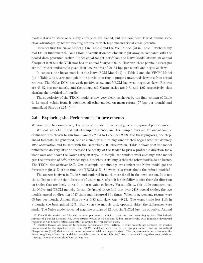
We now start to examine why the proposed model refinements generate improved performance.We look at both in and out-of-sample evidence, and the sample reserved for out-of-sample

evaluation was chosen to run from January 2004 to December 2008. For these purposes, one step-ahead forecasts are generated, one at a time, with a rolling window that begins with the January1986 observation and finishes with the December 2003 observation. Table 7 shows that the modelrefinements do very little to increase the ability of the trader to pick a profitable direction for atrade over and above the Naıve carry strategy. In sample, the random walk exchange-rate modelgets the direction of 58% of trades right, but what is striking is that the other models do no better.The TECM also achieves 58%. Out of sample, the findings are similar: the Naıve model got thedirection right 51% of the time, the TECM 53%. So what is so great about the refined models?

The answer is given in Table 8 and explored in much more detail in the next section. It is notthe ability to pick the right direction of trades more often; it is the ability to pick the right directionon trades that are likely to result in large gains or losses. For simplicity, this table compares justthe Naıve and TECM models. In-sample (panel a) we find that over 2438 pooled trades, the twomodels agreed on direction 1547 times and disagreed 891 times. When in agreement, returns were65 bps per month, Annual Sharpe was 0.83 and skew was −0.23. The worst trade lost 11% ina month, the best gained 12%. But when the models took opposite sides, the differences werestark. The Naıve model collected negative returns of 42 bps, the TECM just the opposite. Annual

20 Even if the entire portfolio churns once per month, which it does not, and assuming typical G10 bid-askspreads of 2 bps for a round trip, these returns would be 55 bps and 82 bps, respectively, with miniscule downwardrevisions in the Sharpe ratios even after allowance for transaction costs.

21 Further tweaks are possible to enhance performance even further. If equal weights are replaced by weightsproportional to the signal strength, the TECM model achieves returns (84 bps per month) and an annualizedSharpe ratios (1.48) that are even more impressive, without negative skew. The improvements occur because thelinear weighting allows the model to re-weight towards more high risk/return trades with negative skew, withoutturning the overall skew significantly negative.

15

Table 7: Fraction of Profitable Trading Positions Correctly Called (%)(a) In sample

Naıve Naıve ECM VAR VECM TECMAustralia 62.9 57.5 56.6 55.5 55.9Canada 57.8 52.0 56.6 55.9 54.8Germany 52.0 53.1 55.9 54.0 56.3Japan 58.2 53.8 61.0 59.9 56.3New Zealand 63.3 59.3 62.1 57.7 58.8Norway 57.1 55.3 57.4 56.6 58.1Sweden 62.7 50.6 66.2 66.2 62.4Switzerland 53.8 54.5 58.1 55.1 58.1UK 53.1 54.9 49.3 53.3 53.9

Pooled 57.9 54.6 58.1 57.1 57.1

(b) Out of sample

Naıve Naıve ECM VAR VECM TECMAustralia 55.0 48.3 53.3 45.0 58.3Canada 43.3 51.7 50.0 46.7 51.7Germany 45.0 46.7 48.3 51.7 45.0Japan 56.7 56.7 65.0 66.7 56.7New Zealand 61.7 60.0 60.0 60.0 60.0Norway 46.7 46.7 58.3 58.3 48.3Sweden 53.3 53.3 56.7 60.0 60.0Switzerland 53.3 55.0 53.3 53.3 55.0UK 45.0 50.0 51.7 51.7 45.0

Pooled 51.1 52.0 55.2 54.8 53.3Note: In sample is 1987 to 2008, out of sample is 2004 to 2008 recursive.

Table 8: When Does the TECM Model Outperform the Naıve Model?(a) In sample N mean s.d. Sharpe skew min max

All trades pooledNaıve 2438 0.0026 0.0297 0.3032 -0.6926 -0.1773 0.1180TECM 2438 0.0057 0.0293 0.6691 0.3674 -0.1100 0.1773

Models agreeNaıve 1547 0.0065 0.0270 0.8345 -0.2272 -0.1100 0.1180TECM 1547 0.0065 0.0270 0.8345 -0.2272 -0.1100 0.1180

Models disagreeNaıve 891 -0.0042 0.0329 -0.4387 -0.9740 -0.1773 0.0744TECM 891 0.0042 0.0330 0.4427 0.9694 -0.0744 0.1773

(b) Out of sample N mean s.d Sharpe skew min max

All trades pooledNaıve 539 -0.0025 0.0315 -0.2721 -1.0580 -0.1773 0.1038TECM 539 0.0028 0.0315 0.3033 0.7006 -0.1056 0.1773

Models agreeNaıve 373 0.0002 0.0278 0.0254 -0.3700 -0.1056 0.1038TECM 373 0.0002 0.0278 0.0254 -0.3700 -0.1056 0.1038

Models disagreeNaıve 166 -0.0085 0.0379 -0.7765 -1.4338 -0.1773 0.0736TECM 166 0.0085 0.0379 0.7765 1.4338 -0.0736 0.1773

Note: In sample is 1987 to 2008, out of sample is 2004 to 2008 recursive. The Sharpe ratio is annualized.

Other statistics are monthly.

16

Sharpes were −0.44 versus 0.44. Skew was −0.97 versus 0.97. Naıve suffered a worst trade of 17%,but the TECM had that on the plus side. TECM’s worst month was only a 7% loss, and that wasNaıve’s best. These results explain why overall, the TECM did better: it avoided crashes, andwhen extreme returns were likely it was better able to pick the right side of the trade. Overallreturns in TECM were 57 versus 26 bps per month for Naıve, Annual Sharpe was 0.67 versus 0.30,and skew was +0.37 versus −0.69.

The out-of-sample results in Table 8 panel (b) apply to the period of the credit crunch andgreat carry trade crash of 2008. These results only amplify the point further. Mean returns werenot that different here, 28 versus −25 bps per month but they were at least up for TECM. Sharpewas +0.30 versus −0.27. Skew was the dramatically different factor in the crisis period: +0.70 forTECM versus −1.17 for the Naıve model.

To sum up, after several stages of refinement, our preferred TECM model surmounts theobjections usually raised to justify excess returns to carry trades. The crudest, naıve long-shortcarry trade strategies, even with currency diversification, deliver Sharpe ratios well below investors’benchmark 1.0 threshold and crash-ridden returns displaying marked negative skew. But byconditioning on the real exchange rate and allowing for nonlinearity, our TECM portfolios deliverhigh returns with a Sharpe ratio 25%–50% above the conventional hurdle for an unexploited riskyarbitrage opportunity.

3 Predictive Ability Evaluation

Is this all too good to be true? Out-of-sample predictive ability testing is the gold standardby which the success or failure of many models in economics is judged. The literature on theability to predict exchange rates spawned by Meese and Rogoff (1983) has been particularlysavage on the field: time and again the invincible random walk has emerged victorious againstan onslaught of ever more sophisticated economic/econometric models of the exchange rate. Themodels investigated in the previous section are promising suitors but they must now face rigorousscrutiny.

The approach that we pursue in this section builds on some standard predictive ability measuresand brings in other techniques that are quite new in economics. Moreover, rather than justevaluating the ability to predict exchange rates per se, we are interested in evaluating a model’sability to generate attractive profits that have high Sharpe ratios and low skewness.

Recall our definition of ex-post nominal excess returns of a long FX position,

mt+1 = ∆et+1 + (i∗t − it)

which we labeled momentum and let mt+1denote the one-period ahead forecast. Since (i∗t − it)is known at time t, then the only source of uncertainty comes from the prediction of ∆et+1. Inpractice, the position an actual trader takes (i.e., determining which currency to borrow in andwhich to invest in) depends on the sign of mt+1 for which we define the dichotomous variabledt+1. This variable takes the value of 1 if mt+1 > 0 and −1 otherwise, so that realized returns can

17

be defined asµt+1 = dt+1mt+1.

Setting the forecasting problem up as a binary choice or direction problem makes sense on acouple of dimensions. First, as a statistical matter, making successful continuous exchange rate(and hence, return) forecasts is a harder challenge, as those working in the Meese-Rogoff traditionhave shown; but a directional forecast sets a lower bar, one that recent work suggests could besurmountable (Cheung, Chinn, and Garcia Pascual 2005). Second, it is all that is needed evenin the case of equal-weight currency portfolios. Thirdly, directional forecasting is important fortraders. Like other funds, currency strategies face the risk of redemptions or closure if negativereturns are frequent and/or large. It is nice to pick the bigger winners, rather than just small ones,but not if the strategy risks blowing up. The point is only amplified when funds are leveraged.Thus from a trader’s point of view, what is often most important is the ability to correctly predictthe profitable direction of the carry trade and for this reason we introduce methods designed toevaluate a model’s ability to correctly classify the data according to direction.

In this section we examine the directional predictive ability of our preferred models in twoways. First, we evaluate the quality of the binary signal itself using new techniques from signaldetection theory. We then evaluate the performance of trading strategies based on the binarysignal, using loss-function methods that can go beyond the prevalent RMSE criterion and insteadbe adapted to metrics of investment performance of interest to traders, like returns, Sharpe, andskewness.

3.1 Hits and Misses: The ROC Curve

Forecasts of a binary outcome are called classifiers. The biostatistics and engineering literaturesprovide techniques, rarely used in economics, for the statistical evaluation of models for classifica-tion (see Pepe, 2003 for a survey). Specifically, the receiver operating characteristic (ROC) curvecharacterizes the quality of a forecasting model and its ability to anticipate correctly the occur-rence and non-ocurrence of pre-defined events.22 For greater detail, we refer readers to anotherpaper where we discuss and develop ROC techniques to evaluate investment performance (Jordaand Taylor 2009).

In our problem the directional outcome variable is dt+1 = sign(mt+1) ∈ {−1, 1}, the ex-postprofitable direction of the currency investment. Let the variable δt+1 to be a scoring classifier suchthat for a given threshold c, δt+1 > c is taken to indicate dt+1 = 1, and δt+1 ≤ c corresponds todt+1 = −1 instead. Our classifier will be the predictions of the conditional means obtained withthe models in Tables 2–5, so that δt+1 = mt+1 but in what follows we maintain the more genericnotation δt+1.

Let TP (c) denote the true positive rate defined as P [δt+1 > c|dt+1 = 1], sometimes also calledsensitivity or recall rate, and in the more familiar Neyman-Pearson nomenclature, 1 minus the

22 The origin of the ROC curve can be traced back to radar signal detection theory developed in the 1950s and1960s (Peterson and Birdsall, 1953), and its potential for medical diagnostic testing was recognized as early as 1960(Lusted, 1960). More recently, ROC analysis has been introduced in psychology (Swets, 1973), in atmosphericsciences (Mason, 1982), and in the machine learning literature (Spackman, 1989).

18

Type II error, or the power of the test (the test here being the ability to correctly identify dt+1 withh(δt+1), for any strictly monotonic function h(.)). Let FP (c) denote the false positive rate definedas P [δt+1 > c|dt+1 = −1] which is 1 minus the specificity or the Type I error, or the size of thetest. Then the ROC curve is defined as the plot of TP (c) against FP (c) for values of c ∈ (−∞,∞).Notice that when c = ∞, TP (c) = FP (c) = 0 and when c = −∞ then TP (c) = FP (c) = 1 sothat the ROC curve can be displayed in [0, 1]× [0, 1] space.

The 45-degree diagonal line corresponds to the ROC curve of a uninformative classifier, where,for any given observation, at any threshold, there is a 50-50 chance of correctly classifying thedirection of trade. In this context, the 45-degree line corresponds to the natural null of the efficientmarkets hypothesis: on average, profitable trades cannot be predicted better than a coin toss andthe classifier contains no information at any threshold. This is a natural benchmark in our analysis.Intuitively, the “better” a classifier is, the closer the ROC curve is to the ideal classifier that hugsthe left and top edges of the unit square (and the further away it is from the 45-degree line). Wenow apply a formal test based on this intuition.

The area under the curve (AUC) measures the probability that the classifier for an observationwhose outcome is dt+1 = 1 attains a higher value than that for an observation whose outcomeis dt+1 = −1, that is P [δ

+

t+1 > δ−t+1] and where the superscript denotes the sign of the true

outcome. Thus, the AUC ranges from 0.5 to 1, since for a simple coin toss the probabilitydescribed previously would be 0.5. (Should any classifier deliver an AUC less than 0.5, its forecastcould simply be inverted!)23

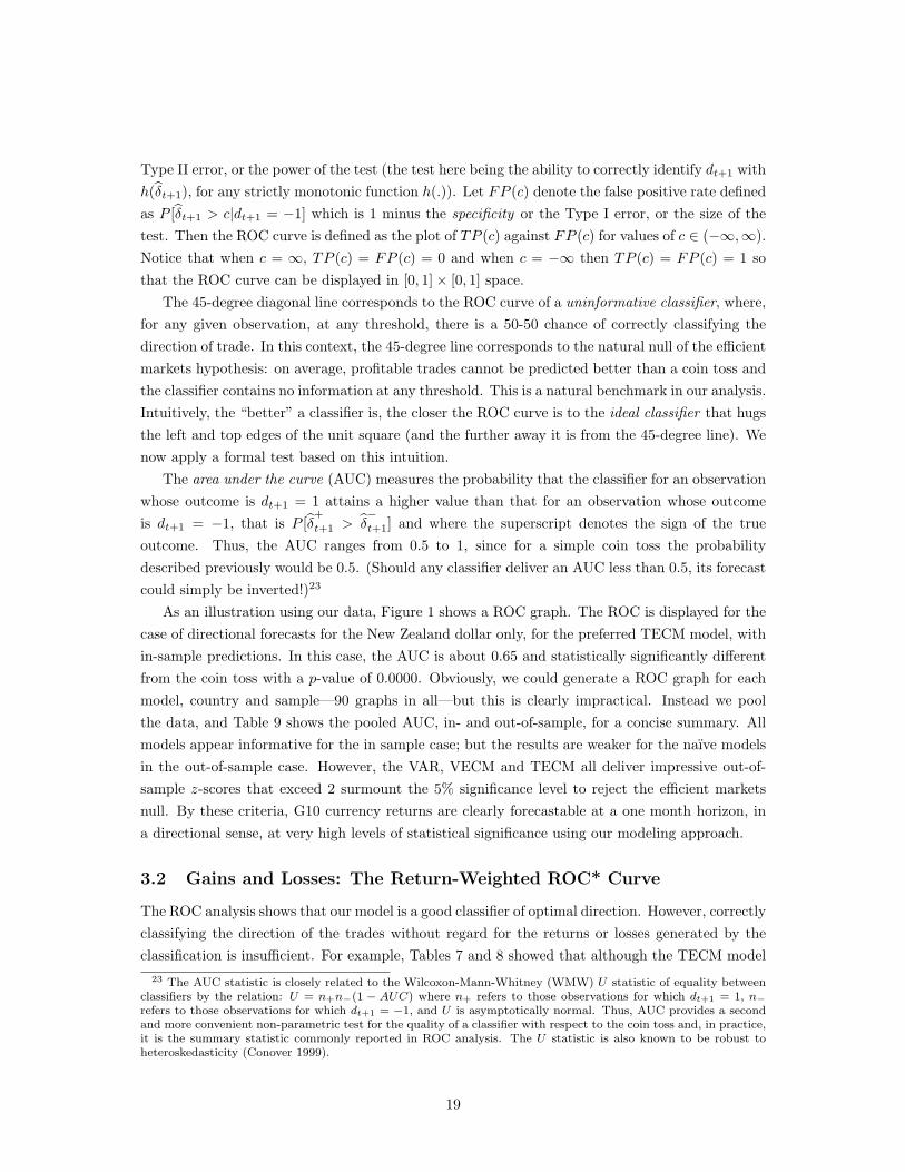
As an illustration using our data, Figure 1 shows a ROC graph. The ROC is displayed for thecase of directional forecasts for the New Zealand dollar only, for the preferred TECM model, within-sample predictions. In this case, the AUC is about 0.65 and statistically significantly differentfrom the coin toss with a p-value of 0.0000. Obviously, we could generate a ROC graph for eachmodel, country and sample—90 graphs in all—but this is clearly impractical. Instead we poolthe data, and Table 9 shows the pooled AUC, in- and out-of-sample, for a concise summary. Allmodels appear informative for the in sample case; but the results are weaker for the naıve modelsin the out-of-sample case. However, the VAR, VECM and TECM all deliver impressive out-of-sample z-scores that exceed 2 surmount the 5% significance level to reject the efficient marketsnull. By these criteria, G10 currency returns are clearly forecastable at a one month horizon, ina directional sense, at very high levels of statistical significance using our modeling approach.

3.2 Gains and Losses: The Return-Weighted ROC* Curve

The ROC analysis shows that our model is a good classifier of optimal direction. However, correctlyclassifying the direction of the trades without regard for the returns or losses generated by theclassification is insufficient. For example, Tables 7 and 8 showed that although the TECM model

23 The AUC statistic is closely related to the Wilcoxon-Mann-Whitney (WMW) U statistic of equality betweenclassifiers by the relation: U = n+n−(1 − AUC) where n+ refers to those observations for which dt+1 = 1, n−refers to those observations for which dt+1 = −1, and U is asymptotically normal. Thus, AUC provides a secondand more convenient non-parametric test for the quality of a classifier with respect to the coin toss and, in practice,it is the summary statistic commonly reported in ROC analysis. The U statistic is also known to be robust toheteroskedasticity (Conover 1999).

19

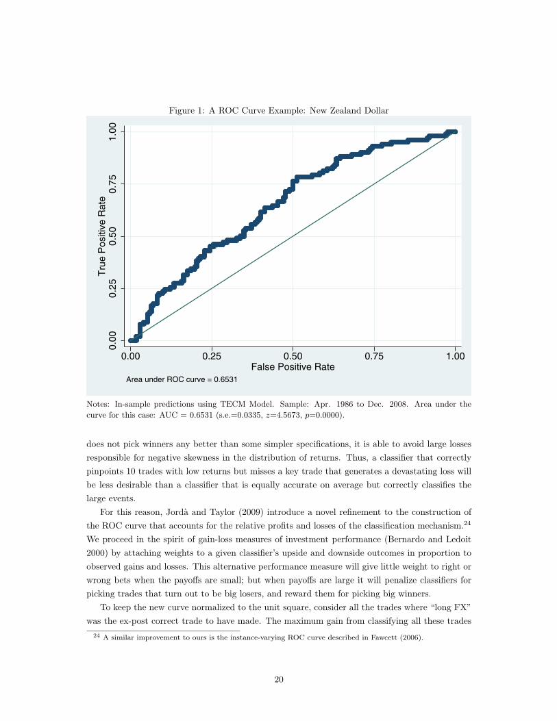
Figure 1: A ROC Curve Example: New Zealand Dollar0

.00

0.2

50

.50

0.7

51

.00

Tru

e P

ositiv

e R

ate

0.00 0.25 0.50 0.75 1.00False Positive Rate

Area under ROC curve = 0.6531

Notes: In-sample predictions using TECM Model. Sample: Apr. 1986 to Dec. 2008. Area under the

curve for this case: AUC = 0.6531 (s.e.=0.0335, z=4.5673, p=0.0000).

does not pick winners any better than some simpler specifications, it is able to avoid large lossesresponsible for negative skewness in the distribution of returns. Thus, a classifier that correctlypinpoints 10 trades with low returns but misses a key trade that generates a devastating loss willbe less desirable than a classifier that is equally accurate on average but correctly classifies thelarge events.

For this reason, Jorda and Taylor (2009) introduce a novel refinement to the construction ofthe ROC curve that accounts for the relative profits and losses of the classification mechanism.24

We proceed in the spirit of gain-loss measures of investment performance (Bernardo and Ledoit2000) by attaching weights to a given classifier’s upside and downside outcomes in proportion toobserved gains and losses. This alternative performance measure will give little weight to right orwrong bets when the payoffs are small; but when payoffs are large it will penalize classifiers forpicking trades that turn out to be big losers, and reward them for picking big winners.

To keep the new curve normalized to the unit square, consider all the trades where “long FX”was the ex-post correct trade to have made. The maximum gain from classifying all these trades

24 A similar improvement to ours is the instance-varying ROC curve described in Fawcett (2006).

20

Table 9: Area Under the ROC CurveModel AUC s.e. z-score p-value

(a) In SampleNaıve 0.5905 0.0115 7.85 0.0000Naıve ECM 0.5604 0.0116 5.19 0.0000VAR 0.5996 0.0115 8.67 0.0000VECM 0.5935 0.0115 8.11 0.0000TECM 0.6084 0.0114 9.47 0.0000

(b) Out of sampleNaıve 0.5170 0.0249 0.68 0.4949Naıve ECM 0.5245 0.0249 0.99 0.3236VAR 0.5654 0.0247 2.65 0.0081VECM 0.5778 0.0246 3.17 0.0015TECM 0.5541 0.0247 2.19 0.0284

Notes: In sample is 1987 to 2008, out of sample is 2004 to 2008 with recursive estimation. The AUCstatistic is a Wilcoxon-Mann-Whitney U -statistic with asymptotic normal distribution and its valueranges from 0.5 under the null to a maximum of 1 (an ideal classifier). See Jorda and Taylor (2009).

correctly with dt+1 = 1 would beBmax =

∑dt+1=1

mt+1.

Now consider all the trades where “short FX” was the ex-post correct trade to have made. Sim-ilarly, the maximum loss from misclassification of these trades, and going long in them, wouldbe

Cmax =∑

dt+1=−1

mt+1.

We can now redefine, or rescale, the true positive and false positive rates TP (c) and FP (c) interms of the upside and downside returns m actually achieved, relative to the maximally attainablegains and losses thus defined. For any given threshold c, this leads to new statistics as follows:

TP ∗(c) =

∑bdt+1=1|dt+1=1mt+1

Bmax; and FP ∗(c) =

∑bdt+1=1|dt+1=−1mt+1

Cmax

The plot of TP ∗(c) versus FP ∗(c) is then, by construction, limited to the unit square, andgenerates what we term a returns-weighted ROC curve, which is denoted the ROC* curve. As-sociated with the ROC* curve is a corresponding return-weighted AUC statistic, denoted AUC*.Intuitively, if AUC* exceeds 0.5 this is evidence that the classifier outperforms the coin toss nullfrom a return-weighted or gain-loss perspective. Detailed derivation of these statistics and theirproperties are provided in Jorda and Taylor (2009), along with techniques for inference.

Using these return-weighted statistics strongly reinforces our argument that classifiers basedon our more refined models (VECM/TECM) are informative; in contrast the performance of themore naıve models are not statistically distinguishable from the coin-toss null. Table 10 collectssummary AUC* statistics for the same in- and out-of-sample periods discussed in Table 9.

The AUC* statistics are higher than the corresponding AUC statistics reported in Table 9,and the z-scores attained are much higher too. The VECM and TECM appear to perform better

21

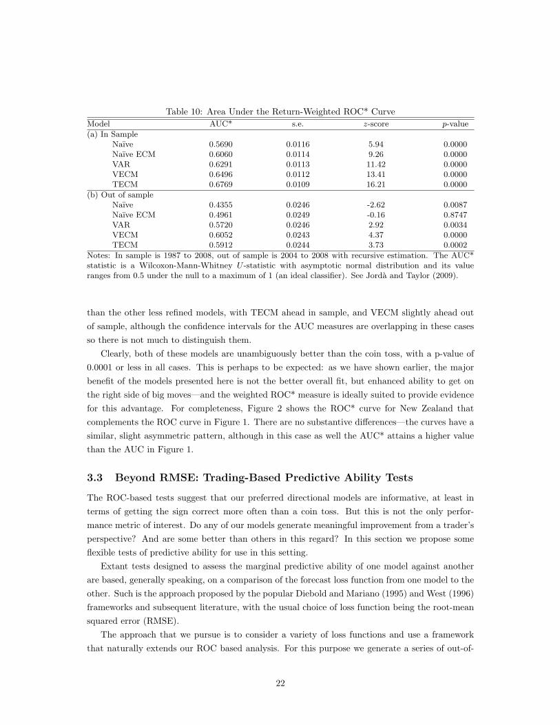
Table 10: Area Under the Return-Weighted ROC* CurveModel AUC* s.e. z-score p-value

(a) In SampleNaıve 0.5690 0.0116 5.94 0.0000Naıve ECM 0.6060 0.0114 9.26 0.0000VAR 0.6291 0.0113 11.42 0.0000VECM 0.6496 0.0112 13.41 0.0000TECM 0.6769 0.0109 16.21 0.0000

(b) Out of sampleNaıve 0.4355 0.0246 -2.62 0.0087Naıve ECM 0.4961 0.0249 -0.16 0.8747VAR 0.5720 0.0246 2.92 0.0034VECM 0.6052 0.0243 4.37 0.0000TECM 0.5912 0.0244 3.73 0.0002

Notes: In sample is 1987 to 2008, out of sample is 2004 to 2008 with recursive estimation. The AUC*statistic is a Wilcoxon-Mann-Whitney U -statistic with asymptotic normal distribution and its valueranges from 0.5 under the null to a maximum of 1 (an ideal classifier). See Jorda and Taylor (2009).

than the other less refined models, with TECM ahead in sample, and VECM slightly ahead outof sample, although the confidence intervals for the AUC measures are overlapping in these casesso there is not much to distinguish them.

Clearly, both of these models are unambiguously better than the coin toss, with a p-value of0.0001 or less in all cases. This is perhaps to be expected: as we have shown earlier, the majorbenefit of the models presented here is not the better overall fit, but enhanced ability to get onthe right side of big moves—and the weighted ROC* measure is ideally suited to provide evidencefor this advantage. For completeness, Figure 2 shows the ROC* curve for New Zealand thatcomplements the ROC curve in Figure 1. There are no substantive differences—the curves have asimilar, slight asymmetric pattern, although in this case as well the AUC* attains a higher valuethan the AUC in Figure 1.

3.3 Beyond RMSE: Trading-Based Predictive Ability Tests

The ROC-based tests suggest that our preferred directional models are informative, at least interms of getting the sign correct more often than a coin toss. But this is not the only perfor-mance metric of interest. Do any of our models generate meaningful improvement from a trader’sperspective? And are some better than others in this regard? In this section we propose someflexible tests of predictive ability for use in this setting.

Extant tests designed to assess the marginal predictive ability of one model against anotherare based, generally speaking, on a comparison of the forecast loss function from one model to theother. Such is the approach proposed by the popular Diebold and Mariano (1995) and West (1996)frameworks and subsequent literature, with the usual choice of loss function being the root-meansquared error (RMSE).

The approach that we pursue is to consider a variety of loss functions and use a frameworkthat naturally extends our ROC based analysis. For this purpose we generate a series of out-of-

22

Figure 2: A ROC∗ Curve Example: New Zealand Dollar0

.2.4

.6.8

1R

etu

rn W

eig

hte

d T

rue

Po

sitiv

e R

ate

0 .2 .4 .6 .8 1Return Weighted False Positive Rate

Notes: In-sample predictions using TECM Model. Sample: Apr. 1986 to Dec. 2008. Area under the

curve for this case: AUC* = 0.6631 (s.e.=0.0347, z=4.6941, p=0.0000)

sample, one-period ahead forecasts from a rolling sample of fixed length. It is clear that in thistype of set-up, estimation uncertainty never vanishes and for this reason we adopt the conditionalpredictive ability testing methods introduced in Giacomini and White (2006). These tests have theadvantage of permitting heterogeneity and dependence in the forecast errors, and their asymptoticdistribution is based on the view that the evaluation sample goes to infinity even though theestimation sample remains of fixed length.

Specifically, let {Lit+1}T−1

t=R denote the loss function associated with the sequence of one step-ahead forecasts, where R denotes the fixed size of the rolling estimation-window from t = 1 toT − 1, and let i = 0, 1 (with the index 0 indicating forecasts generated with the unit root nullmodel and the index 1 indicating the alternative model). Then, the test statistic

GW1,0 =∆L

σL/√P

d→ N(0, 1) (4)

23

provides a simple test of predictive ability, where

∆L =1P

T−1∑t=R

(L1

t+1 − L0t+1

);

and

σL =

√√√√ 1P

T−1∑t=R

(L1

t+1 − L0t+1

)2(since E(∆L) = 0 under the null. See theorem 1 in Giacomini and White, 2006); and whereP = T −R+ 1.

The flexibility in defining the loss function permitted in the Giacomini and White (2006)framework is particularly useful for our application. The framework extends naturally to a panelcontext, where the forecasts for N different currencies over P periods are pooled together. Inthat case, assuming independence across units in the panel we may implement the above test withthe observation count P replaced by NP . Because one may suspect that the panel units are notindependent, we implement a cluster-robust covariance correction however.

The traditional summary statistic of predictive performance is the well-known root-meansquared error

RMSEi =

√√√√ 1P

T−1∑t=R

(mit+1 −mt+1)2; i = 0, 1

where mit+1 = Et(mt+1|Model= i) for i = 0, 1. Thus, one can assess whether differences in RMSE

between models are statistically significant by choosing

Lit+1 =

(mi

t+1 −mt+1

)2; i = 0, 1.

But even if RMSE is a major focus of the academic literature, it is of little interest to those infinancial markets, since models with good (poor) fit measured by RMSE could still generate poor(respectively, good) returns. So what about investors’ preferred performance criteria? Fortunately,the flexibility of the framework allows one to consider loss functions based on alternative metrics.Three natural ways to assess the advantages of different models from the perspective of the tradesthey generate are as follows:

First, the average return, defined for the evaluation sample as

RTNi =1P

T−1∑t=R

µit+1; i = 0, 1.

Second, the Sharpe ratio, defined for the evaluation sample as

SRi =1P

∑T−1t=R µi

t+1√1P

∑T−1t=R

(µi

t+1 − µi)2

; i = 0, 1.

24

Table 11: Forecast Evaluation: Loss-Function Statistics for Pooled DataRMSE RTN SR SK(×100) (annual %) (annual) (monthly)

(a) In sample, 1987–2008

Naıve 2.93 3.23 1.08 -0.77NECM 2.91 4.16 1.32 0.06VAR 2.89 5.42 1.83 -0.26VECM 2.87 6.46 2.19 0.24TECM 2.83 7.35 2.42 0.34

(b) Out of sample, 2004–2008

Naıve 2.23 -2.84 -1.01 -1.00NECM 2.22* -0.80 -0.21 -0.36VAR 2.21 2.23* 0.72 -0.17*VECM 2.20 3.70* 1.22 0.44*TECM 2.20 3.27* 0.92 0.64*

Notes: * indicates the GW statistic against the Naıve null based on the corresponding loss function,is significant at the 95% confidence level. To correct for cross-sectional dependence, a cluster-robustcovariance correction is used. See text.

Third, and finally, the skewness of realized returns

SKi =

√P (P − 1)P − 2

1P

∑T−1t=R

(µi

t+1 − µi)3

(1P

∑T−1t=R

(µi

t+1 − µi)2)3/2

; i = 0, 1.

where µi = 1P

∑T−1t=R µi

t+1 for i = 0, 1. Thus, this Sharpe ratio measures the out-of-samplerisk/return profile of the carry trade strategies implied by competing forecasting models, whereasthe skewness coefficient allows us to assess the models’ ability to avoid infrequent but particularlylarge negative returns. The associated loss functions are derived as in the case of the RMSE andsummarized in the appendix for completeness.

Table 11 summarizes the full in-sample and the out-of-sample loss functions: RMSE (in per-cent); Annualized Return (in percent); Annualized Sharpe Ratio; and the monthly Skewnesscoefficient for each of the models in Tables 2, 3, and 5; that is the Naıve (null); the Naıve ECM;the VAR, the VECM; and the TECM models. For panel (b), which contains the out-of-sampleresults, an asterisk indicates that the Giacomini-White (2006) statistic associated to the loss func-tion in that column is significant at the conventional 95% confidence level (as compared to theNaıve model in row 1). Results for pooled month-year observations are shown. The results incolumn 1 show that the difference in the models as judged by RMSE are miniscule. However,measured by metrics that matter to traders, the differences are considerable. For example, in ourpreferred model, in-sample the difference in annual mean returns is +3.23 for Naıve versus +7.35percent for TECM. Out-of-sample the period includes the period of carry trade crashes, and thedifference is −2.84 versus +3.45 percent (panel b). Annual Sharpe Ratios for pooled returns areboosted from +1.08 to +2.42 in-sample, and from −1.01 to +0.92 in the turbulent out-of-sampleperiod. Skewness improves from −0.77 to +0.34 in-sample, and from −1.0 to +0.64 out-of-sample.There is little doubt which of these returns a currency hedge fund manager would have preferred.

25

The GW tests also show that, with the exception of skewness, these performance improvementsare statistically significant, out-of-sample, relative to the Naıve model.

4 Alternative Crash Protection Strategies

In this section we compare the merits of our fundamentals-based model with the recent literature,where two alternative crash protection strategies have emerged. The first is a contract-basedstrategy: Burnside, Eichenbaum, Kleshchelski, and Rebelo (2008ab) explore a crash-free tradingstrategy where FX options are used to hedge against a tail event that takes the form of a collapsein the value of the high-yield currency. The second is a model based strategy: Brunnermeier et al.(2008) argue that an important cause of carry trade crashes is the arrival of a state of the worldcharacterized by an increase in market volatility or illiquidity.

4.1 Options

In Burnside, Eichenbaum, Kleshchelski, and Rebelo (2008ab) a naıve carry trade strategy is thestarting point. Traders go long the high yield currencies and short the low yield currencies. Thefocus is also on major currencies, as here, although the sample window goes back to the 1970sera of capital controls, and applies to a larger set of 20 currencies. Returns may be computed forindividual currencies, portfolios, of for subsets of currencies (e.g., groups of 1, 2 or 3 highest yieldcurrencies against similar groups of lowest yield currencies). However, each naıve strategy can beaugmented by purchase of at-the-money put options on the long currencies.25

This augmentation leads to positive skew by construction. It averts tail risk, but at a price.How large is that price? For the 1987/1 to 2008/1 period a naıve unhedged equally-weighted carrytrade had a return of 3.22% per annum with an annualized Sharpe ratio of 0.54 and a skewness of-0.67. This compares with the U.S. stock market’s 6.59% return, 0.45 Sharpe ratio, and skewnessof -1.16 over the same period. Normality of returns is rejected in both cases.

Implementing the options-based hedged carry trade boosts the Sharpe ratio a little, eliminatesthe negative skew, but at a significant cost. Added insurance costs of 0.71% per annum mean thatthe hedged strategy lowers returns to only 2.51% annually, has a Sharpe of 0.71, and a significantpositive skew of 0.75. Thus on an annualized basis the hedged strategy costs 80 bps, and still failsto bring the Sharpe close to the mythical 1.0 hurdle.

In contrast, let us now compare our similar equal-weight naıve carry trading strategy with ournonlinear fundamentals-based return-forecast strategy, in Table 6, panel (a). Comparing Models(1) and (5), our strategy increases returns from 29 to 46 bps per month, and still eliminatesnegative skew. For comparison, on an annualized basis, the return rises from 3.45% to 5.55%, again of 210 bps, with a Sharpe ratio of 1.34. Unlike the options-based strategy, our approach canincrease returns and lower skew at the same time.

We make some further observations. To be fair, we recognize that the strategies implementedby Burnside, Eichenbaum, Kleshchelski, and Rebelo (2008ab) are crude and mainly illustrative.

25 This strategy is also studied by Bhansali (2007).

26

The options they employ are at-the-money, and push skew into strong positive territory. Inreality, investors might purchase option that are more out-of-the-money; at much lower costs, thiscould protect against only the large crashes, yet still eliminate the worst of the negative skew(Jurek 2008). Nonetheless, even if lower cost option strategies are found, our results suggest thatthere is a better no-cost way to hedge against crashes by using data on deviations from long-runfundamentals, and this information also serves to boost absolute returns and Sharpe ratios too.Moreover, options contracts have other drawbacks, many of which were shown to be salient issuesafter the financial crash of 2008. Option prices embed volatility, so in periods of turmoil the priceof insurance can rise just when it is most needed, depending on the implied FX volatility (Bhansali2007). And as with all derivatives, options carry counterparty risk. In addition, options price andposition data from exchanges may not be representative, since this activity represents only atiny fraction of FX option trading, the vast majority being over-the-counter. Also, like forwardsand futures derivatives, options carry bid-ask spreads that can explode such as to make marketsdysfunctional in crisis periods. Finally, whilst Burnside, Eichenbaum, Kleshchelski, and Rebelo(2008ab) show the viability of an options-based strategy for 20 widely-traded major currencies,FX derivative markets are thin to nonexistent for many emerging market currencies, and bid-ask spreads can be wide, so in those markets currency strategists may have to seek alternativeplain-vanilla approaches, like ours, that might help avert currency crash risk.

4.2 VIX Signal

In Brunnermeier et al. (2008) it is argued that various forms of generalized asset market distress,by reducing risk appetite, may be significant contributors to carry trade crashes. The logic of theargument is that such conditions may prompt a pull back from all risky asset classes, leading toshort-run losses via order flow effects, or the price impact of trades. To provide empirical supportfor this proposition the authors show that, on a weekly basis, changes in the VIX volatility index(a proxy for distress) correlate with the returns to naıve carry trade strategies—that is, tradingstrategies which do not condition on any information except the interest differential. An increase inVIX was found to correlate with lower carry trade returns, all else equal, suggesting that liquidityrisk might partially explain the excess returns. However, lagged changes in VIX had little or nopredictive power for next periods returns. This prompts us to explore whether the same argumentshold true in our sample, and if we detect any difference when we use our preferred trading strategy.We found that in our data, using the same 1992–2006 sample period, at a monthly frequency, therewas no evidence that the change in VIX was correlated with returns contemporaneously, nor thatit helped predict next period’s returns.

Specifically, in the spirit of Brunnermeier et al. (2008), we computed loadings of the returnson the contemporaneous and lagged change in VIX. We first regressed the actual (signed) returnsof trades based on the naıve model on the contemporaneous change in VIX for all months andall currencies in our data over their sample period 1992–2006. We then did the same for thelagged change in VIX. We then re-ran both regressions using the actual (signed) returns of ourpreferred TECM model. In none of the four regression was the slope coefficient significant, and

27

in all cases it actually had the “wrong” positive sign, suggesting that rising VIX was slightlypositively correlated with profits this month, or next month.

We make some further observations. To be fair, we should note that Brunnermeier et al. (2008)present these results at a weekly frequency. In our dataset, we have to work at monthly frequencygiven the underlying price index data used to construct the real exchange rate fundamental signal.We conjecture that the VIX signal may have stronger correlations with current or future returns atweekly or even fortnightly frequency, even when placed in a model like ours augmented to accountfor real exchange rate fundamentals, although further research is warranted in this area.

If the sample is extended using our full dataset, including through the volatile crisis periodin 2007–2008, the coefficients are not stable and we do sometimes find a statistically significantrole for VIX signals in predicting negative actual (signed) returns of the naıve Model 1, althoughthis episode is outside the window considered by Brunnermeier et al. (2008). But this resultdisappears, and the sign even reverses, when we include the real exchange rate term and use ourpreferred TECM model, suggesting that the real exchange rate deviation alone may serve as anadequate crash warning. In fact, in these models the sign of the coefficient on the change inVIX was often positive and significant, suggesting potentially the opposite interpretation: whenVIX is rising, arbitrage capital may be being withdrawn, but this has a tendency to leave moreprofits on the table for the risk tolerant, or “patient capital,” and for traders pursuing profitablefundamental-based strategies with inherent skew protection of the sort developed here.

5 Reality Check: Exchange Traded Funds

Beyond out-of-sample forecasting, an alternative way to judge our preferred modeling and tradingstrategies against the naıve benchmark is to compare the recent performances of different currencyfunds in the real world. When comparing the merits of naıve versus fundamentals-based strategies,the relative performance of these funds in the financial crisis 2008 proves to be very revealing.

First, we seek a fund representative of the naıve long-short approach, the basic carry strategiesof Burnside, Eichenbaum, and Rebelo (2008), and the same authors with Kleshchelski (2008ab),henceforth BER/K. For this purpose we focus on the Deutsche Bank G10 Currency Harvest USDIndex (AMEX: DBCFHX, Bloomberg: DBHVG10U). This index has been constructed back toMarch 1993 using historical data. Since April 2006 this index has been made available to retailinvestors—in the United States, for example, it trades as the Powershares DB G10 CurrencyHarvest Fund (AMEX: DBV). These indices track a portfolio based on 2:1 leveraged currencypositions selected from ten major “G10” currencies with the U.S. dollar as a base. For every $2invested, the index goes long (+$1) in the three currencies with the highest interest rates, andshort ($-1) in the three with the lowest interest rates, and with 0 invested in the other three,with $1 placed in Treasuries for margin. The portfolio is reweighted only every quarter and isimplemented via futures contracts. If the U.S. dollar is one of the long or short currencies, thatposition makes no profit in the base currency and is dropped, so leverage falls to 1.66.

This ETF’s naıve approach to forecasting any currency pair via the carry signal matches theBER/K approach. The main differences are that the index is not equal weight and tries to pick

28

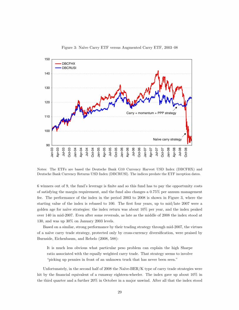
Figure 3: Naıve Carry ETF versus Augmented Carry ETF, 2003–08

90

100

110

120

130

140

150

Jan-

03

Apr

-03

Jul-0

3

Oct

-03

Jan-

04

Apr

-04

Jul-0

4

Oct

-04

Jan-

05

Apr

-05

Jul-0

5

Oct

-05

Jan-

06

Apr

-06

Jul-0

6

Oct

-06

Jan-

07

Apr

-07

Jul-0

7

Oct

-07

Jan-

08

Apr

-08

Jul-0

8

Oct

-08

DBCFHXDBCRUSI

Naïve carry strategy

Carry + momentum + PPP strategy

Notes: The ETFs are based the Deutsche Bank G10 Currency Harvest USD Index (DBCFHX) and

Deutsche Bank Currency Returns USD Index (DBCRUSI). The indices predate the ETF inception dates.

6 winners out of 9, the fund’s leverage is finite and so this fund has to pay the opportunity costsof satisfying the margin requirement, and the fund also changes a 0.75% per annum managementfee. The performance of the index in the period 2003 to 2008 is shown in Figure 3, where thestarting value of the index is rebased to 100. The first four years, up to mid/late 2007 were agolden age for naıve strategies: the index return was about 10% per year, and the index peakedover 140 in mid-2007. Even after some reversals, as late as the middle of 2008 the index stood at130, and was up 30% on January 2003 levels.

Based on a similar, strong performance by their trading strategy through mid-2007, the virtuesof a naıve carry trade strategy, protected only by cross-currency diversification, were praised byBurnside, Eichenbaum, and Rebelo (2008, 588):

It is much less obvious what particular peso problem can explain the high Sharperatio associated with the equally weighted carry trade. That strategy seems to involve“picking up pennies in front of an unknown truck that has never been seen.”

Unfortunately, in the second half of 2008 the Naıve-BER/K type of carry trade strategies werehit by the financial equivalent of a runaway eighteen-wheeler. The index gave up about 10% inthe third quarter and a further 20% in October in a major unwind. After all that the index stood

29

below its January 2003 level of 100, and four and a half years of gains had been erased.Could a more sophisticated carry trade strategy have avoided this carnage, whilst still pre-

serving positive returns overall? Yes. To see this we now look for a different index which matchesbetter with our more sophisticated trading strategy. We focus on the Deutsche Bank CurrencyReturns USD Index (Bloomberg: DBCRUSI). This investible index operates on the same set of“G10” currencies but amalgamates three different trading signals for each currency, where againthe signals are +1 (long), 0 (no position), and –1 (short). The first signal is the same as before: thenaıve carry trade signal based purely on the interest rate, the 3-month LIBOR rate (The “CarryIndex”), updated every three months. The second signal is based a calculation of the deviation ofthat currency from its FEER level, based on continuously updated common-currency price levelsfrom the OECD (The “Valuation Index”) updated every three months. The third signal is basedon momentum, and takes into account the USD return to holding that currency in the previousperiod (The “Momentum Index”) updated every month. Clearly this augmented carry strategyis much closer in spirit to our augmented models, given its mix of signals. In our model “carry”corresponds to the lagged interest differential; “momentum” corresponds mostly to the laggedexchange rate change (given persistence in the interest differential); and “valuation” correspondsto our monthly real exchange rate deviation.

The Deutsche Bank Currency Returns index is not currently available as an exchange tradedfund in the U.S., but it is traded as an ETF in Frankfurt. A test of our approach is to ask:did investors in this more sophisticated fund fare better in 2008 than those invested in the naıveDBV fund. As Figure 3 shows, they did much better. On the 2003–07 upswing this index wasless volatile, but returns were still strong, up about 28% at the peak. Momentum signals gotthe money quickly out of crashing currencies (and back in when they rose), and valuation signalshedged against dangerously overvalued currencies (and jumped in otherwise), tempering the naıvecarry signal. The real test was in 2008. The index did remarkably well: performance was absolutelyflat returns, and kept 20% of the cumulative gains locked in. Looking at the three components ofthis strategy, a 30%+ loss on the carry signal in 2008, was offset by a 10% gain on the PPP signaland a 20% gain on the momentum signal.

Notice how the relative performance of these ETFs closely matches the results of our tradingstrategies as shown back in Table 7. In the out of sample results the Naıve-BER/K type modelshowed a loss of 2.84% per year from 2004 to 2008. Our more sophisticated VECM showed a gainof 4.15% per year. That differential of 7% per year would cumulate to a roughly 30% divergencein index values over a four year period. Despite some differences in methods between our modelsimulations and the ETFs, this is almost exactly the cumulative divergence seen for the real-worldETFs in Figure 3.

Fundamentals matter. Comparing the two ETFs makes clear the gains from using a moresophisticated currency strategy incorporating a FEER measure. Although academic research hasfocused on the naıve strategies, it is no secret in the financial markets that more refined models,taking into account the signals discussed here and many others, are actively employed by seriousfund managers and are now leaking out into traded products.26

26 For example, in addition to the Deutsche Bank ETs, see also the FX Currents from Goldman Sachs.

30

6 Conclusion

The international financial crisis of the second half of 2008 effectively undid the majority of thepersistent carry trade returns observed during the previous five to ten years. Strategies based onarbitraging interest rate differentials across countries under the belief that it was equiprobable forexchange rates to appreciate or depreciate displayed consistently positive average returns. Butthese returns were volatile and subject to occasional crashes (negative skewness). It can be arguedthen, that the observation of persistent carry trade returns does not violate the efficient marketshypothesis.

This paper instead shows that more sophisticated strategies that incorporate information aboutthe fundamental equilibrium exchange rate can deliver positive returns with high Sharpe ratiosand zero or even mildly positive skewness. We do not claim to be better at forecasting exchangerates than the ubiquitous random walk model in Meese and Rogoff (1983). We claim that we canpredict better than the toss of a coin the direction of the carry trade that will produce positivereturns. Our results indicate that this is no in-sample fluke and in fact, a thorough out-of-sampleanalysis that includes the turbulent period of the second-half of 2008, reaffirms the robustness ofour claims. Moreover, the historical performance of real-world ETFs during this period (discussedin the previous section) corroborates our findings.

In addition to these findings, our paper makes two contributions to the empirical assessmentof the directional predictive potential of alternative investment strategies. On the one hand, weadapt formal predictive ability tests with loss functions that better represent those characteristicsthat are most important to an investor, which do not necessarily correspond with those that havebeen traditionally important to an econometrician. Moreover, we introduce in this paper newtechniques commonly used in biostatistics, the ROC curve and associated statistics, that are ofconsiderable utility for investors. In a companion paper we have extended the discussion of thetechniques introduced here in several dimensions. For instance, among some of the topics we cover,we discuss how to evaluate more sophisticated trading strategies that allow for long-short-cashpositions (Jorda and Taylor 2009).

We believe that there is more work to be done that builds on the foundations of this paper. Inthis paper we have considered simple portfolio strategies based on equal- or return-tuned-weights,but clearly strategies that exploit the time-varying correlation structure across countries beg formore sophisticated portfolio designs. Similarly, a lesson from the ROC analysis introduced in thispaper is that directional prediction can be fine-tuned to reflect the marginal trade-offs betweenreturn, volatility, and skew encapsulated in each investor’s preferences.

However, both of these extensions naturally beg the question: Whither the efficient marketshypothesis?

31

Appendix

The loss functions of the Giacomini-White (2006) statistic in expression (4) corresponding to each of the

three trading-based metrics are, for returns:

Lit+1 = bµi

t+1; i = 0, 1;

for the Sharpe ratio

Lit+1 =

bµit+1q

1P

PT−1t=R

`bµit+1 − µi

´2 ; i = 0, 1;

and for skewness, we use Pearson’s second definition of skewness to provide a comparable scale with the

returns- and Sharpe ratio-based loss functions, specifically

Lit+1 =

3`bµi

t+1 − µi(0.50)´q

1P

PT−1t=R

`bµit+1 − µi

´2 ; i = 0, 1

where µi(0.50) refers to the median of bµit+1 for t = R, ..., T − 1. The cluster correction that we use for

the panel consists in computing the covariance matrix of the loss function difference across countries and

standardizing by the inverse of its Cholesky decomposition.

References

Alexius, Annika. 2001. Uncovered Interest Parity Revisited. Review of International Economics 9(3):

505–17.

Bakker, Age, and Bryan Chapple. 2002. Advanced Country Experiences with Capital Account Liberal-

ization. Occasional Paper 214, Washington, D.C.: International Monetary Fund.

Bacchetta, Philip, and Eric van Wincoop. 2006. Can Information Heterogeneity Explain the Exchange

Rate Determination Puzzle? American Economic Review 96(3): 552–76.

Bekaert, Geert, and Robert J. Hodrick. 1993. On Biases in the Measurement of Foreign Exchange Risk

Premiums. Journal of International Money and Finance 12(2): 115–38.

Bernardo, Antonio E., and Ledoit, Olivier. 2000. Gain, Loss and Asset Pricing. Journal of Political

Economy 108(1): 144–72.

Bhansali, Vineer. 2007. Volatility and the Carry Trade, Journal of Fixed Income 17(3): 72–84.

Brunnermeier, Markus K., Stefan Nagel, and Lasse H. Pedersen. 2008. Carry Trades and Currency

Crashes. NBER Working Papers 14473.

Burnside, A. Craig. 2007. The Cross-Section of Foreign Currency Risk Premia and Consumption Growth

Risk: A Comment. NBER Working Papers 13129.

Burnside, A. Craig, Martin Eichenbaum, Isaac Kleshchelski, and Sergio Rebelo. 2006. The Returns to

Currency Speculation. NBER Working Papers 12489.

Burnside, A. Craig, Martin Eichenbaum, Isaac Kleshchelski, and Sergio Rebelo. 2008a. Do Peso Problems

Explain the Returns to the Carry Trade? CEPR Discussion Papers 6873, June.

Burnside, A. Craig, Martin Eichenbaum, Isaac Kleshchelski, and Sergio Rebelo. 2008b. Do Peso Problems

Explain the Returns to the Carry Trade? NBER Working Papers 14054.

Burnside, A. Craig, Martin Eichenbaum, and Sergio Rebelo. 2007. The Returns to Currency Speculation

in Emerging Markets. NBER Working Papers 12916.

32

Burnside, A. Craig, Martin Eichenbaum and Sergio Rebelo. 2008. Carry Trade: The Gains of Diversifi-

cation. Journal of the European Economic Association 6(2-3): 581–88.

Cheung, Yin-Wong, Menzie D. Chinn, and Antonio Garcia Pascual. 2005. Empirical Exchange Rate

Models of the Nineties: Are Any Fit to Survive? Journal of International Money and Finance 24(7):

1150–75.

Chinn, Menzie D., and Jeffrey A. Frankel. 2002. Survey Data on Exchange Rate Expectations: More

Currencies, More Horizons, More Tests. In Monetary Policy, Capital Flows and Financial Market

Developments in the Era of Financial Globalisation: Essays in Honour of Max Fry, edited by W.

Allen and D. Dickinson. London: Routledge, 145–67.

Clarida, Richard, and Daniel Waldman. 2007. Is Bad News About Inflation Good News for the Exchange

Rate? NBER Working Papers 13010.

Clinton, Kevin. 1998. Transactions Costs and Covered Interest Arbitrage: Theory and Evidence. Journal

of Political Economy 96: 358–70.

Coakley, Jerry, and Ana Marıa Fuertes. 2001. A Non-linear Analysis of Excess Foreign Exchange Returns.

Manchester School 69(6): 623–42.

Conover, W. J. 1999. Practical Nonparametric Statistics. 3rd edition. New York: John Wiley and Sons.

Diebold, Francis X., and Roberto S. Mariano. 1995. Comparing Predictive Accuracy. Journal of Business

and Economic Statistics 13(3): 253–63.

Dominguez, Kathryn M. 1986. Are Foreign Exchange Forecasts Rational? New Evidence from Survey

Data. Economics Letters 21(3): 277–81.

Dooley, Michael P., and Jeffrey R. Shafer. 1984. Analysis of Short-Run Exchange Rate Behavior: March

1973 to 1981. In Floating Exchange Rates and The State of World Trade and Payments, edited by

David Bigman and Teizo Taya, 43–70.

Engel, C., and James D. Hamilton. 1990. Long Swings in the Dollar: Are They in the Data and Do

Markets Know It? American Economic Review 80(4): 689–711.

Fackler, Martin. 2007. Japanese Housewivwes Sweat in Secret as Markets Reel. New York Times,

September 16, 2007.

Fama, Eugene F. 1984. Forward and Spot Exchange Rates. Journal of Monetary Economics 14(3):

319–38.

Fawcett, Tom. 2006. ROC Graphs with Instance-Varying Costs. Pattern Recognition Letters 27(8):

882–91.

Fisher, Eric O’N. 2006. The Forward Premium in a Model with Heterogeneous Prior Beliefs. Journal of

International Money and Finance 25(1): 48–70.

Frankel, Jeffrey A. 1980. Tests of Rational Expectations in the Forward Exchange Market. Southern

Economic Journal 46(4): 1083–1101.

Frankel, Jeffrey A., and Kenneth A. Froot. 1987. Using Survey Data to Test Standard Propositions

Regarding Exchange Rate Expectations. American Economic Review 77(1): 133–53.

Frenkel, Jacob A., and Richard M. Levich. 1975. Covered Interest Rate Arbitrage: Unexploited Profits?

Journal of Political Economy 83(2): 325–38.

Froot, Kenneth A., and Jeffrey A. Frankel. 1989. Forward Discount Bias: Is It an Exchange Risk

Premium? The Quarterly Journal of Economics 104(1): 139–61.

Froot, Kenneth A., and Tarun Ramadorai. 2008. Institutional Portfolio Flows and International Invest-

ments. Review of Financial Studies 21(2): 937–71.

33

Froot, Kenneth A., and Richard H. Thaler. 1990. Foreign Exchange. Journal of Economic Perspectives

4(3): 179–92.

Fujii, Eiji, and Menzie D. Chinn. 2000. Fin de Siecle Real Interest Parity. NBER Working Papers 7880.

Giacomini, Raffaella, and Halbert White. 2006. Tests of Conditional Predictive Ability. Econometrica

74(6): 1545–78.

Granger, Clive W. J., and Timo Terasvirta. 1993. Modelling Nonlinear Economic Relationships. Oxford:

Oxford University Press.

Hansen, Lars Peter, and Robert J. Hodrick. 1980. Forward Exchange Rates as Optimal Predictors of

Future Spot Rates: An Econometric Analysis. Journal of Political Economy 88(5): 829–53.

Ilut, Cosmin. 2008. Ambiguity Aversion: Implications for the Uncovered Interest Rate Parity Puzzle.

Northwestern University. Photocopy.

Jeanne, Olivier, and Andrew K. Rose. 2002. Noise Trading And Exchange Rate Regimes. Quarterly

Journal of Economics 117(2): 537–69.

Jorda, Oscar, and Alan M. Taylor. 2009. Investment Performance of Directional Trading Strategies.

University of California, Davis. Photocopy.

Jurek, Jakub W. 2008. Crash-Neutral Currency Carry Trades. Princeton University. Photocopy.

Levich, Richard M., and Lee R. Thomas, III. 1993. The Significance of Technical Trading-Rule Profits in

the Foreign Exchange Market: A Bootstrap Approach. Journal of International Money and Finance

12(5): 451–74.

Lusted, Lee B. 1960. Logical Analysis in Roentgen Diagnosis. Radiology 74: 178–93.

Lustig, Hanno, and Adrien Verdelhan. 2007. The Cross Section of Foreign Currency Risk Premia and

Consumption Growth Risk. American Economic Review 97(1): 89–117.

Lyons, Richard K. 2001. The Microstructure Approach to Exchange Rates. Cambridge, Mass.: MIT Press.

Mason, Ian B. 1982. A Model for the Assessment of Weather Forecasts. Australian Meterological Society

30: 291–303.

Meese, Richard A., and Kenneth Rogoff. 1983. Empirical Exchange Rate Models of the Seventies. Journal

of International Economics 14(1–2): 3–24.

Michael, Panos, A. Robert Nobay, and David A. Peel. 1997. Transactions Costs and Nonlinear Adjustment

in Real Exchange Rates: An Empirical Investigation. Journal of Political Economy 105(4): 862–79.

Obstfeld, Maurice, and Alan M. Taylor. 1997. Nonlinear Aspects of Goods-Market Arbitrage and Adjust-

ment: Heckscher’s Commodity Points Revisited. Journal of the Japanese and International Economies

11(4): 441–79.

Obstfeld, Maurice, and Alan M. Taylor. 2004. Global Capital Markets: Integration, Crisis, and Growth.

Cambridge: Cambridge University Press.

Pedroni, Peter. 1999. Critical Values for Cointegration Tests in Heterogeneous Panels with Multiple

Regressors. Oxford Bulletin of Economics and Statistics 61: 653–70.

Pedroni, Peter. 2004. Panel Cointegration: Asymptotic and Finite Sample Properties of Pooled Time

Series Tests with an Application to the PPP Hypothesis. Econometric Theory 20(3): 597–625.

Pepe, Margaret S. 2003. The Statistical Evaluation of Medical Tests for Classification and Prediction.

Oxford: Oxford University Press.

Pesaran, M. Hashem, Yongcheol Shin, and Ronald P. Smith. 1999. Pooled Mean Grouped Estimation of

Dynamic Heterogeneous Panels. Journal of the American Statistical Association 94: 621–24.

Peterson, W. Wesley, and Theodore G. Birdsall. 1953. The Theory of Signal Detectability: Part I. The

General Theory. Electronic Defense Group, Technical Report 13, June 1953. Available from EECS

34

Systems Office, University of Michigan.

Plantin, Guillaume, and Hyun Song Shin. 2007. Carry Trades and Speculative Dynamics. Princeton

University. Photocopy.

Pojarliev, Momtchil, and Richard M. Levich. 2007. Do Professional Currency Managers Beat the Bench-

mark? NBER Working Papers 13714.

Pojarliev, Momtchil, and Richard M. Levich. 2008. Trades of the Living Dead: Style Differences, Style

Persistence and Performance of Currency Fund Managers. NBER Working Papers 14355.

Poterba, James M., and Lawrence H. Summers. 1986. The Persistence of Volatility and Stock Market

Fluctuations. American Economic Review 76(5): 1142–51.

Pritchard, Ambrose Evans. 2007. Goldman Sachs Warns of Dead Bodies After Market Turmoil. The

Daily Telegraph, June 3, 2007.

Sager, Michael, and Mark P. Taylor. 2008. Generating Currency Trading Rules from the Term Structure

of Forward Foreign Exchange Premia. University of Warwick, October. Photocopy.

Sarno, Lucio, and Mark P. Taylor. 2002. The Economics of Exchange Rates. Cambridge: Cambridge

University Press.

Sarno, Lucio, Giorgio Valente, and Hyginus Leon. 2006. Nonlinearity in Deviations from Uncovered

Interest Parity: An Explanation of the Forward Bias Puzzle. Review of Finance 10(3): 443–82.

Shleifer, Andrei, and Robert W. Vishny. 1997. A Survey of Corporate Governance. Journal of Finance

52(2): 737–83.

Silvennoinen, Annastiina, Timo Terasvirta, and Changli He. 2008. Unconditional Skewness from Asym-

metry in the Conditional Mean and Variance. Department of Economic Statistics, Stockholm School

of Economics. Photocopy.

Sinclair, Peter J. N. 2005. How Policy Rates Affect Output, Prices, and Labour, Open Economy Issues,

and Inflation and Disinflation. In How Monetary Policy Works, edited by Lavan Mahadeva and Peter

Sinclair. London: Routledge.

Spackman, Kent A. 1989. Signal Detection Theory: Valuable Tools for Evaluating Inductive Learning. In

Proceedings of the Sixth International Workshop on Machine Learning. Morgan Kaufman, San Mateo,

Calif., 160–63.

Swets, John A. 1973. The Relative Operating Characterstic in Psychology. Science 182: 990–1000.

Taylor, Alan M., and Mark P. Taylor. 2004. The Purchasing Power Parity Debate. Journal of Economic

Perspectives 18(4): 135–58.

Taylor, Mark P., David A. Peel, and Lucio Sarno. 2001. Nonlinear Mean-Reversion in Real Exchange

Rates: Toward a Solution to the Purchasing Power Parity Puzzles. International Economic Review

42(4): 1015–42.

West, Kenneth D. 1996. Asymptotic Inference about Predictive Ability. Econometrica 64(5): 1067–84.

35