The California Cooperative Remote Sensing Project: Final ... · THE CALIFORNIA COOPERATIVE REMOTE...
106
NASA Technical Memorandum 100073 The California Cooperative Remote Sensing Project: Final Report Christine A. Hlavka and Edwin J. Sheffner (liASA-TlI-100G73| _£]_ E&LI]FO_Illil CGGPB_RA_ZVE IEfBO_E SBliSIiiG }]B(J_,Ct Final Ee_o[t (ililSJ) $_ P CSCL 08B G3/_ 3 B89-13824 July 1988 rU/ A National Aeronautics and Space Administration https://ntrs.nasa.gov/search.jsp?R=19890004453 2020-04-08T12:02:54+00:00Z
Transcript of The California Cooperative Remote Sensing Project: Final ... · THE CALIFORNIA COOPERATIVE REMOTE...

NASA Technical Memorandum 100073
The California CooperativeRemote Sensing Project:Final Report
Christine A. Hlavka and Edwin J. Sheffner
(liASA-TlI-100G73| _£]_ E&LI]FO_Illil CGGPB_RA_ZVEIEfBO_E SBliSIiiG }]B(J_,Ct Final Ee_o[t (ililSJ)$_ P CSCL 08B
G3/_ 3
B89-13824
July 1988
rU/ ANational Aeronautics andSpace Administration
https://ntrs.nasa.gov/search.jsp?R=19890004453 2020-04-08T12:02:54+00:00Z


NASA Technical Memorandum 100073
The California CooperativeRemote Sensing Project:Final Report
Christine A. Hlavka, Ames Research Center, Moffett Field, California
Edwin J. Sheffner, TGS Technology, Inc., Moffett Field, California
July 1988
I_IASANational Aeronautics andSpace Administration
Ames Research CenterMoffett Field, California 94035


TABLE OF CONTENTS
SUMMARY ........................................................................ I
I. INTRODUCTION ............................................................... 3
2. BACKGROUND ................................................................. 5
2.1 Landsat Data .......................................................... 5
2.2 The USDA Use of Landsat Data .......................................... 6
2.2.1 The June Enumerative Survey .................................... 6
2.2.2 EDITOR Data Processing ......................................... 6
2.2.2.1 JES data encodement ................................... 7
2.2.2.2 Landsat data processing ............................... 8
2.2.2.3 Estimation ............................................ 9
2.2.3 EDITOR History ................................................. 11
2.3 CDWR Use of Landsat Data .............................................. 12
3. THE COOPERATIVE AGREEMENT .................................................. 15
3.1 Project Goals and Participating Organizations ......................... 15
3.1.1 Planning Sessions .............................................. 16
3.1.2 Ground Surveys ................................................. 16
3.1.3 Landsat Data ................................................... 17
3.1.4 Landsat Data Processing ........................................ 17
3.1.5 Software Support ............................................... 17
3.1.6 Data Communications ............................................ 19
3.1.7 Landsat Data Products .......................................... 21
3.2 Early Research Tasks .................................................. 21
3.2.1 The Small Grains Task .......................................... 21
3.2.2 The Multi-Crop Task ............................................ 23
3.3 Development of MIDAS .................................................. 24
3.3.1 Workstation Configuration ...................................... 25
3.3.2 Workstation Communications ..................................... 25
3.3.3 Workstation Software ........................................... 27
3.3.3.1 CIE and ELAS .......................................... 27
3.3.3.2 PEDITOR ............................................... 27
3.4 Plan for the 1985 Inventory ........................................... 28
3.4.1 Technical Approach ............................................. 28
3.4.2 Role of Participating Organizations ............................ 30
3.4.3 Preparations ................................................... 31
3.4.3.1 PEDITOR testing ....................................... 31
3.4.3.2 Code written for CCRSP ................................ 32
3.4.3.3 Current year photography .............................. 32
4. THE 1985 INVENTORY ......................................................... 33
4.1 The Test Site ......................................................... 33
4.2 Ground Data Acquisition ............................................... 36
PRI_CED[NG PAGE BLANK NO_ FILMI_ iii

4.2.1 June Enumerative Survey........................................ 364.2.2 Transect Survey................................................ 364.2.3 Preparation of the Survey Data................................. 38
4.3 Landsat Data Preparation .............................................. 394.3.1 Landsat Data Acquisition ....................................... 394.3.2 Reformatting of Landsat Scenes................................. 404.3.3 Formatting Landsat Coverage of SegmentData.................... 42
4.4 Landsat Data Processing and Interpretation ............................ 424.4.1 Training for Classification .................................... 424.4.2 Statistics File Editing ........................................ 434.4.3 Classification and Aggregation ................................. 44
4.5 Estimation ............................................................ 454.5.1 The Original Landsat Estimates ................................. 454.5.2 Revised Estimates .............................................. 494.5.3 Experimental Estimates ......................................... 52
4.6 Landsat MapProducts .................................................. 634.7 Data System Performance............................................... 65
4.7.1 PEDITORSoftware ............................................... 664.7.2 Other MIDASSoftware ........................................... 664.7.3 MIDASHardware................................................. 674.7.4 BBN/EDITOR..................................................... 674.7.5 Networking ..................................................... 67
5. ANALYSISOF INVENTORYDATA................................................. 695.1 Data System Performance............................................... 695.2 Accuracy Assessment................................................... 70
6. CONCLUSIONSANDRECOMMENDATIONS............................................ 736.1 Data Processing ........................................................ 73
6.1.1 Implementation of PEDITOR....................................... 736.1.2 Processing Environment.......................................... 746.1.3 Data System Recommendations..................................... 74
6.2 Use of Landsat Data................................................... 756.2.1 Acreage Estimates .............................................. 756.2.2 Landsat MapProducts ........................................... 77
APPENDIXA - PEDITORMODULESANDFUNCTIONSAS OF2/20/87 ....................... 79
APPENDIXB - RECOMMENDATIONSFORTHE1985 INVENTORY............................ 81
APPENDIXC - ROBUSTREGRESSIONESTIMATION...................................... 87
REFERENCES..................................................................... 92
iv

LIST OF TABLES AND FIGURES
Table I:
Table 2:
Table 3:
Table 4:
Table 5:
CCRSP Hardware and Software Systems .................................. 18
1985 Inventory--Data Processing of ARC ............................... 34
California Area Frame Strata Definitions ............................. 37
Landsat Acquisitions for 1985 Central Valley Inventory ............... 41
1985 California JES Area Frame Population and Sample Sizes ........... 46
Table 6: Regression Parameters for Acreage Estimates (a) AD42
Table 6: Continued (b) AD43
Table 6: Concluded (c} AD44
Table 7: Comparison of Several Types of Landsat Estimates for Rice
and Walnuts with CCLRS Estimates
Table 8A: Landsat Acreage Estimates: Alfalfa ................................... 53
Table 8B: Landsat and CCLRS Acreage Estimates:
Table 8C: Landsat and CCLRS Acreage Estimates:
Table 8D: Landsat and CCLRS Acreage Estimates:
Table 8E: Landsat and CCLRS Acreage Estimates:
Table 8F: Landsat and CCLRS Acreage Estimates:
Table 8G: Landsat and CCLRS Acreage Estimates:
Table 8H: Landsat and CCLRS Acreage Estimates:
Table 8I: Landsat and CCLRS Acreage Estimates:
Table 8J: Landsat and CCLRS Acreage Estimates:
Table 9:
Almonds ........................ 54
Corn ........................... 55
Cotton ......................... 56
Grains (Wheat and Barley) ...... 57
Grapes ......................... 58
Rice ........................... 59
Tomatoes ....................... 60
Treefruit ...................... 61
Walnuts ........................ 62
Robust Estimates of Regression Parameters
Figure I: CCRSP Network ........................................................ 20
Figure 2: MIDAS System Configuration ........................................... 26
Figure 3: Central Valley Inventory - Data Processing Steps ..................... 29
Figure 4:1985 Central Valley Inventory - Study Site and Landsat Frame
Locations ............................................................ 35


pRaiSING PAGE WLANK Nf_ PILM]_ ",__Li\_
viii ORIGINAE PA_
COLOR PHOTOGRAPH


THE CALIFORNIA COOPERATIVE REMOTE SENSING PROJECT:
FINAL REPORT
Christine A. Hlavka
NASA Ames Researh Center
and
Edwin J. Sheffner
TGS Technology, Inc.
SUMMARY
The U.S. Department of Agriculture (USDA), the California Department of Water
Resources (CDWR), the Remote Sensing Research Program of the University of Califonia
(UCB) and the National Aeronautics and Space Administration (NASA) completed a 4-yr
cooperative project on the use of remote sensing in monitoring California agricul-
ture. This report is a summary of the project and the final report of NASA's con-
tribution to it. The cooperators developed procedures that combined the use of
Landsat Multispectral Scanner imagery and digital data with ground survey data for
area estimation and mapping of the major crops in California. An inventory of the
Central Valley was conducted as an operational test of the procedures. The satel-
lite and survey data were acquired by USDA and UCB and processed by CDWR and NASA.
The inventory was completed on schedule--demonstrating the plausibility of the
approach, although further development of the data processing system is necessary
before it can be used efficiently in an operational environment.
(Photograph at left shows crop-specific classification of the entire California
Central Valley completed using Landsat digital data. A 35mm slide of this
photograph is included in this paper and is located in the envelope attached to the
inside back cover.)


I. INTRODUCTION
If California were a separate nation, it would have the fifth largest economy
in the world. The foundation of the California economy is agriculture. Exploiting
the advantages of a virtual year long growing season, massive irrigation projects,
abundant tillable land and a variety of soil types and microclimates, Californians
grow commercially over 200 different crops.
The agricultural resource is monitored closely. The responsibility lies with
several state and federal agencies including the California Department of Water
Resources (CDWR) and the National Agricultural Statistics Service (NASS), formerly
the Statistical Reporting Service (SRS), of the U.S. Department of Agriculture
(USDA). A tally of irrigated lands and estimates of water use is annually compiled
by CWR. Because water demand varies with crop type, CDWR conducts crop inventories
as well. Annual crop inventories are conducted by NASS as part of its mandate from
Congress to collect and distribute state and national agricultural statistics. Both
agencies support research on methods to improve data collection and processing
procedures so that the required information can be obtained more efficiently and
with greater accuracy.
In 1982 a cooperative agreement was signed by CDWR, NASS, the Remote Sensing
Research Program of the University of California, Berkeley (UCB) and the National
Aeronautics and Space Administration (NASA) - Ames Research Center (ARC). The long-
range (4-yr) goal of the joint research project was to develop procedures for area
estimation and mapping of the major crops in California using Landsat digital data
as the primary data source. The principal funding agency was NASS.
The joint research project was conducted in four stages, each stage correspond-
ing, generally, to a fiscal year (FY):
FY83 - Evaluation of inventory techniques
FY84 - Design of inventory experiment
FY85 - Perform operational test of inventory procedure
FY86 - Evaluate procedure performance
The following report is a summary of the work done under the auspices of the
cooperative agreement. The 1985 inventory experiment and the work performed at ARC
in support of it are emphasized. The joint research project was truly coopera-
tive. Participants met regularly, worked together closely, and shared responsibil-
ity. Although a Joint report on results would have been appropriate, at the request
of NASS, separate reports on the 1985 inventory are being submitted by ARC, UCB, and
CDWR. This report focuses on the contributions and responsibilities of the staff at
ARC--specifically, the Ecosystem Science and Technology Branch (ECOSAT: NASA code
SEE).
In the course of preparing for the 1985 inventory, many specific research tasks
were completed. Some tasks had significance beyond the context of the cooperative
agreement and have been reported on separately. Those tasks are referred to in the

report, and the results are summarized. The reader should consult the referencesfor a more detailed report on specific accomplishments.
The body of the report is divided into five sections. The "Background" pro-vides a description of Landsat and a summaryof how NASSand CDWRprocessed andapplied Landsat data prior to the cooperative agreement. "The Cooperative Agree-ment" describes how the agencies worked together, the goals of the project, thetasks assigned to ARCand the evolution of research within the project. Section 4,"The 1985 Inventory," is a review of the design, implementation and evaluation ofthe 1985 inventory experiment. The report ends with "Conclusions and Recommenda-tions," as seen from the perspective of ARC.
The California Cooperative RemoteSensing Project involved a great many
people. The project was conceived and supported by Bill Caudill (NASS), Bob
MacGregor (CCLRS), Glen Sawyer (CDWR) and Ethel H. Bauer (ARC). Management and
technical assistance was provided by Bill Pratt (NASS), Richard Sigman (NASS),
Randall W. Thomas (UCB), Ron Radenz (CCLRS), Dave Kleweno (CCLRS), George May
(CCLRS) and James G. Lawless (ARC). The core programming staff included Martin Ozga
(NASS), Martin Holko (NASS), Anthony Travlos (UCB), Paul Ritter (UCB), Robert Slye
(NASA), and Gary Angelici (Sterling Software). The primary responsibility for data
collection, processing and analysis for the 1985 inventory fell to Jay Baggett
(CDWR). He was aided by Catherine Brown (UCB), Louisa Beck (UCB), Charles Ferchaud
(CDWR) and others.
Assistance with the preparation of the manuscript was provided by Honoris
Ocasio (TGS Technology).
The authors wish to express their appreciation for the efforts of all those who
contributed to this undertaking.
4

2. BACKGROUND
The efforts of the four organizations involved in the CCRSPwere not joined bychance but were based on a recent history of commoninterests and cooperative workin remote sensing and application of satellite data.
2.1 Landsat Data
Landsat is the nameof a series of earth observing satellites developed by NASAto monitor renewable and nonrenewable resources. All Landsat satellites are polarorbiting and provide repeat, daytime observations of any area on Earth every
16 days. The multispectral scanner (MSS} aboard Landsat collects imagery from
reflected light from the earth's surface in four ranges of wavelengths in the elec-
tromagnetic spectrum. These spectral bands are: MSS4: 0.4 _m to 0.5 _m (visual
green); MSSS: 0.6 _m to 0.7 _m (visual red); MSS6: 0.7 _m to 0.8 _m (near infra-
red)_ and MSS7: 0.8 _m to 1.1 _m (near infrared). Bands MSS5, MSS6, and MSS7 are
particularly useful in observations of vegetation because chlorphyll absorbs red
light and the mesophyllic tissue in plant leaves reflects near infrared radiation.
Approximately 10 million picture elements, or pixels, make up a Landsat scene. Each
pixel represents the reflectance from 0.8 acre on the ground, and the full scene
roughly covers a square area of about 10,O00 square miles.
The location of a scene is specified by path and row numbers. A path is traced
out by the north to south orbital motion of the satellite during daylight hours on a
given day within the 16-day cycle. These paths, which overlap slightly and cover
the globe, are cut into rows of scenes, so that each row corresponds to an interval
in latitude.
Landsat scenes of the United States (U.S.) are distributed through the Eros
Data Center, and may be obtained as photo products or in digital form on computer-
compatible tapes (CCTs). Scenes on tape are encoded in four brightness levels,
corresponding to the four MSS bands, for each pixel. The tapes are formatted in
such a way that the locations of the brightness levels for each pixel, in terms of
file number on the tape, record number and byte, are a function of the Landsat scene
coordinates (Space Oblique Mercator, or SOM). These coordinates are essentially the
scan number within the scene, and position within the scan line. The SOM coordi-
nates can be calibrated to latitude and longitude, or to Universal Transverse Merca-
tor (UTM) coordinates by using information about the location and attitude of Land-
sat relative to the earth contained on the tape (ref. I). Greater precision is
achieved from calibrations based on regression analysis of sample points whose
location are known in both SOM and ground coordinates. The calibration-control-
point information is usually obtained by the user of the data by measurements on the
Landsat imagery and on high-quality maps, such as the 7.5-min quadrangles at
1:24,000 scale available from U.S. Geological Survey (USGS). Landsat tapes of some
areas also contain some control-point information (refs. 1,2). Because the orbit
and attitude of Landsat are not perfectly stable, the calibration may differ
5

slightly between acquisitions of a scene. If more than one Landsat acquisition is
used in a study of an area, the SOM coordinates of one acquisition are chosen as the
standard coordinates for the study and other Landsat acquisitions are "registered"
to the standard. This means that the coordinates of the other scenes are calibrated
to the standard, and the file(s) containing brightness data are then reformatted, or
"resampled," so that the coordinate systems of all Landsat acquisitions are now the
same. Sometimes other geographical data used in the study is also registered to the
standard SOM coordinate system.
The features of the Landsat system: the spatial resolution, the repeat cover-
age, the spectral resolution, the coverage per scene, the reasonable cost, and the
availability of the data in both photographic and digital formats, make the data
potentially useful in an agricultural inventory.
2.2 The USDA Use of Landsat Data
The USDA, through NASS (SRS), began using Landsat data in the mid 1970's.
Landsat imagery is used routinely now as an aid in development of sampling frames
for crop and livestock inventories, and Landsat digital data have been used to
improve the precision of crop-acreage estimates. Both activities have been in
support of the June Enumerative Survey (JES)--the primary mechanism for obtaining
large area crop estimates in the U.S.
2.2.1 The June Enumerative Survey
The JES is a survey conducted annually by state (ref. 3). Plots are selected
for survey by a stratified random sample (refs. 3,4). Each state is divided into
strata based on land use. Strata boundaries are first drawn on enlargements of
Landsat imagery and/or aerial photography then transferred to medium-scale maps,
usually county highway maps. The area in square miles of each stratum within a
county is tabulated.
A random sample of segments, parcels of land usually one square mile in area,
is drawn from those strata containing a significant amount of agriculture. Segment
boundaries are located on large-scale aerial photography. The photographs are given
to enumerators who visit the sites during the JES. The enumerators draw in the
field boundaries on the aerial photography and identify the contents of the field
primarily through interviews with farmers, and secondarily through windshield sur-
veys. The crop/land-use type may be a crop {e.g., wheat, sorghum, tree fruit,
etc.), natural feature (e.g., grass, pasture, etc.), or nonagricultural land use
(e.g., commercial, industrial, urban, farmstead). The survey data is used to
develop acreage estimates for major crops, by proration by area, i.e. direct expan-
sion (ref. 4).
2.2.2 EDITOR Data Processing
In the latter half of the 1970's, USDA developed a procedure for generating
improved area estimates using Landsat digital data in conjunction with the JES data

(ref. 5). Landsat imagery is interpreted by computer using a statistical classifi-cation algorithm to label pixels according to crop type or land use. The inter-preted imagery is then integrated with digitized geographic boundaries, i.e., JESstratum and segmentboundaries, to create tables of pixel counts by crop type/landuse. The tables are then correlated and integrated with the JES data to form acre-age estimates. The agency uses the Landsat esti_tes to supplement the prorationestimates.
Becauseof the volume of data in a Landsat scene (about 40 million pieces ofinformation) and the combination of data sources involved in the procedure,automated data processing was a prerequisite for area estimation with Landsat.EDITORis a software system developed by USDAto perform the data processingrequired for the Landsat acreage-estimation procedure° EDITORis based on proce-dures developed at Purdue University and implementedwith an image-processing systemcalled LARSYS. LARSYStechniques were adapted for use with JES survey data tocreate EDITOR.
EDITORis a modular system orginally written in Sail, Fortran, Rational Fortran(Ratfor), and Macro prograrmning languages (refs. 6,7). Data are passed betweenmodules by writing and reading files. A feature of EDITOR,possibly unique at thetime of its creation, is the ability to process a variety of types of data coded intext or binary format.
Three categories of data are manipulated in EDITOR- ground data, Landsat dataand statistical data. Ground data consists of information on the location, size,contents and condition of specific fields, and the numberof ground sample segmentsby county, stratum and analysis district. The ground data is maintained in formatssuitable for data processing. Landsat digital data is stored on tape as full orhalf scenes, or is stored on disk in files containing all the data for the segmentsbeing analyzed, the data for specified crop types only, or files in which the datahas been classified. Statistical data is generated by operations on the ground dataand Landsat data.
EDITORwasused by NASSwith sometechnical support provided by ARC. Portionsof EDITORwere also used at ARCfor research on applications of remote sensing.
The data flow within EDITORis summarizedbelow. The EDITORapproach to dataprocessing and a version of the EDITORsoftware were used by CCRSP(refs. 5-8).
2.2.2.1 JES data encodement- Much of the manipulation of ground data files is
completed prior to integration with Landsat data. The data collected by the JES
enumerators, i.e. the per field information collected from the ground sample seg-
ments, are encoded in ground truth files. These files are created in a binary
format on a system outside of EDITOR, and are read by EDITOR modules when the acre-
age estimates are calculated.
Additional files required for the integration of Landsat data with the JES
survey are created and used within EDITOR. The boundaries of the JES strata within
each county are digitized, a process that converts the information marked on a map

to a digital format. The boundaries of each stratum are treated as polygons. Alatitude and longitude for each vertex of a polygon is recorded along with a labelassociating the polygon with a stratum. Files containing polygon data are referredto as "network files." Longitude and latitude coordinates are calibrated to LandsatSOMcoordinates so that the pixels in the scene can be associated with strata. Thenetwork files are reformatted to form EDITOR"mask files" so that counts of Landsatpixels within boundaries can be made. In a similar manner, the boundaries and croptype/land use for each field in the JES segments are digitized and encoded in maskfiles.
2.2.2.2 Landsat data processing- Landsat data is processed to generate pixel
counts for each crop type to be included in the acreage report. The estimation
technique requires pixel counts both by segment and by stratum. The computationally
intensive steps required to generate pixel counts by stratum are performed on a
supercomputer.
For the sake of computational efficiency, the Landsat data is prepared in two
formats for processing in the EDITOR system. The computer is then "trained" to
recognize crop/land-use type on the JES segments. The Landsat imagery is inter-
preted by the computer and classified imagery is generated. Finally, pixels are
counted on the classified imagery with reference to the mask files. These steps in
Landsat data processing are described in the following text.
The first type of reformatting is for processing steps associated with JES
strata and is performed with software outside of EDITOR. The information in Landsat
computer compatible tapes is rearranged so that the brightness values associated
with pixels on each scan line on a scene are contained in a single record. Some-
times data from two Landsat observations of a scene are used. As mentioned in
section 2.1, the Landsat coordinates vary between two observations. This problem is
corrected for by a process called "registration," in which the coordinates of one
observation are calibrated to the coordinates of the other. The USDA procedure
involves location of control points on both observations of the scene. The first
few points are located manually, and then a hundred or so are located with an
automated technique on a supercomputer. The brightness for both dates is then
interleaved so that eight numbers are associated with each pixel.
After the Landsat scene has been reformatted, the data are extracted for the
segments located in the scene. The segment(s) specific digital data is the input
for the the second type of reformatting, termed "packing." Packing is one of the
unique features of EDITOR. A packed file contains a compressed version of a multi-
dimensional histogram, i.e., the number of pixels for each vector of brightness
values by segment or by crop/land-use type (as identified by JES enumerators).
The computer is "trained" to recognize crop/land-use type by a process called
"clustering" performed on Landsat data packed by crop/land-use type. A cluster can
be thought of as a subtype of the crop/land-use type. Each cluster is determined by
a combination of factors that affect the appearance of a patch of ground on Landsat
imagery. These factors include agricultural practices and soil color. The probabi-
listic distribution of brightnesses for each crop/land-use type is modeled as a
8

mixture of multivariate normal (Gaussian) distributions (ref. 9) in which each
normal distribution represents a cluster. In EDITOR, an algorithm called CLASSY
(ref. 10) divides the pixels into groups, or clusters, so that the shape of the
multidimensional histogram, or scattergram, of brightness values for the cluster
conform to the that expected for a normal distribution. The number of pixels, band
means, and covariance matrix of each cluster are evaluated and assembled, with the
crop/land-use type and a number label for the cluster, in a cluster statistics
file. A separate cluster statistics file is developed for each Landsat path,
because the acquisition dates differ among paths. Each Landsat path is considered a
separate "analysis district."
Classification of Landsat imagery is performed by maximum likelihood discrimi-
nation (refs. 7,9,11). Each pixel is labeled with the number of the cluster it most
closely resembles. Resemblance to a cluster is defined as the likelihood of obser-
vation of the brightness values of the pixel if it belonged to the cluster, that is,
if the combination of crop/land-use type and other conditions associated with the
cluster were true for that pixel. The likelihood is highest near the cluster
mean. In subsequent steps, to derive acreage estimates and map products, pixels are
associated with a crop/land-use type, i.e, the type associated with the cluster
number in the cluster statistics file.
"Aggregation" is the tabulation by cluster number of all the pixels in the area
defined by a EDITOR mask file. Aggregation is performed to get pixel counts on
strata within each county of a survey, and within each JES segment. The aggrega-
tions are used to compute acreage estimates.
2.2.2.3 Estimation- Regression estimates (ref. 4, Chapter 7) make use of two
sources of information about the geographical distribution of crops: sampled crop
acreages collected as part of JES, and counts of Landsat pixels labeled by crop on
classified imagery. Estimation on a regional scale is performed in three steps in
EDITOR. A linear relationship between Landsat pixel counts and ground acreage is
developed by regression analysis of the classified segment data and JES statis-
tics. The relationship is then applied to pixel counts on classified, full frame,
Landsat imagery. In the final step, the estimates for all analysis districts are
combined to create a state level estimate for each crop of interest (ref. 12).
Estimation on the county scale is performed by a single module in EDITOR. The
estimates are described in the following text.
If the land-use map were perfectly accurate, then crops' acreages could be
calculated by multiplying the pixels counts by the pixel area (0.8 acres/pixel).
Because there is significant errors in the classification, regression is used to
estimate the relationship between pixels and acres. Regional estimates are derived
by least squares estimates of mean acreage Yh for a given crop per segment (square
mile) on each land use stratum h within each Landsat analysis district, or path, as
follows:
Est(Yh) = Yh + bh × (Xh - Xh) (la)

or, equivalently as:
with:
Est(Y h) : bO + b I × Xh (Ib)
and:
bo : Yh - bh x x h
b I : b h
where xh and Xh are JES sample and population (entire strata within the analysis
district) pixel counts per segment, Yh is the mean JES sample acreage, and bh is
derived from least squares estimation. The estimate of total acreage is computed as
N x Est(Yh) where N is the area of stratum h in square miles, that is, the
number of segments required to cover the stratum.
This type of estimate is generally more accurate than direct expansion wherein
total acreage is estimated by (N/n) x Yh' because Landsat pixels counts are used to
correct for the difference in crop prevalence between the sample and the population
(stratum/path) as a whole.
The improvement in accuracy depends on the correlation r between pixels and
acreage, that is, the variance of Est(Y h) is approximately
[(I - n/N)/N][I - r2]Vary which can be compared to a variance of [(I n/N)/N] [Vary]for a direct expansion e_timate.
These estimates are then summed over strata and analysis districts to form the
regional crop estimates. The standard error for each estimate is computed using the
standard formula (ref. 4, Chapter 7). Each estimate is statistically independent of
the others, therefore the standard error for the regional estimates are computed by
root mean squares of sums of standard errors for the district/stratum estimates.
Equation (I) defines a linear relationship between the Est(Y h) and Xh. A low
value (less than 0.8) of the slope term bh compensates for a tendency for other
crops or types of land use to be identified as the crop of interest in the Landsat
classification. Conversely, a tendency for the Landsat classification to
under-identify the crop is corrected by a high value for bh. Usually, bh is
computed on each stratum/path, thus allowing for possibly different patterns of
confusion among crops and land use types.
County estimates are derived using a modification of standard least squares
regression developed by Battese and Fuller (refs. 13-15), with NASS support and
collaboration. The intercept in equation (I) is altered on a per county basis, in
the estimation of parameters for a linear model of the relationship between acreage
Y and pixels X includes a "county effect." In ordinary least squares regression,
the regression line goes through the means point x,y, as in equation (I). The
10

Battese-Fuller (B-F) line, lies between the line in equation (I) and a parallel
straight line going through county means point:
Y : Yh,c + bh × (Xh,c - Xh,x,c) (2)
The position of the B-F line is determined by a factor d as follows:
Est(Yh,c) : Yh + bh x (Xh, c - Xh, c) + d × D(3)
where D is the vertical distance between lines (I) and (2). The factor d is
computed to minimize the standard error of the estimate. This value of d turns
out to be the proportion of the variance(VAR) in the residuals of equation (I) due
to "county effect":
d : VAR(between counties)/VAR(total) (4)
The value of Est(Y h) is computed using equation (3) and then adjusted so that
the estimates of total acreage for the counties in an analysis district add up to
the regional estimate. County estimates are formed by summing district/stratum B-F
estimates in the same way the regional estimates are computed.
2.2.3 EDITOR History
The first Landsat satellite was launched in 1972. The following year, NASS
began development of EDITOR. The system was completed in 1978. EDITOR was used
first, and has been most successful, for crop area estimates in the Midwestern
states. Large field size, relatively short growing seasons, and the small number of
crops grown make the Midwest particularly suitable for inventories with Landsat
data. One acquisition per Landsat scene is sometimes sufficient to be able to
identify the crop(s) being surveyed. The NASS program with EDITOR expanded so that
by 1983 Landsat based estimates for seven states were being generated annually.
EDITOR was written at the Center for Advanced Computation at the University of
Illinois in association with NASS and ARC. It has undergone amendment and modifica-
tion since 1978 at NASS and ARC, but the basic processing steps have not changed.
In the early 1980's EDITOR was operated by NASS on a PDPIO computer at Bolt,
Berenek, and Newman (BBN) in Cambridge, Massachusetts. The more computationally
intensive procedures were performed on the Cray computer at ARC. At that time, the
agency made a decision to rewrite the software resident on the BBN system so that it
could be operated on a number of different machines. Because ARC was familiar with
EDITOR, NASS contracted with NASA to undertake the bulk of the recoding. Work on
the new code, called PEDITOR for portable EDITOR, began in 1983.
PEDITOR was completed to the satisfaction of NASS in 1985. It was installed on
an IBM system for agency use with a link to a commercially operated Cray computer.
All, or part, of PEDITOR has been implemented on a VAX 11/780 (VMS), a SUN2 worksta-
tion (UNIX), and the MIDAS workstations (XENIX) at ARC, UCB, and CDWR. PEDITOR was
used by CCRSP for the Central Valley inventory in 1985. Much is written about
11

PEDITORand the MIDASworkstation in the following pages. The PEDITORand MIDASprojects occurred concurrently with CCRSP,and several staff membersfrom NASS,ARCand UCBworked on more than one of the projects. However, the three projects wereadministratively and managerially separate. The decisions taken by CCRSP,discussedbelow, to use PEDITORas the primary data processing package for the 1985 inventoryand to attempt to perform most of the data processing on MIDASmeant that the fateof the three projects becameintertwined. PEDITORand MIDASare discussed in somedetail in this report because it is impossible to evaluate the results of the 1985inventory without knowledgeof the history and operational characteristics of thehardware and software systems used.
2°3 CDWRUse of Landsat Data
Amongits manyachievements, California is the most populous state, the mostexpensive state in which to live, and the state with the most comprehensive programof water management. Water managementis mandatedby the needs of agriculture andthe peculiar propensity of Californians to settle where the water isn't--approximately 75%of the state's population lives south of the Tehachapi Mountainsin a region that recieves only 10%of the state's annual precipitation. Since 1957,the state has operated under a m_ster plan for the development and allocation of itswater resources. The CDWRwas assigned the task by the State Legislature of period-ically updating and supplementing the plan.
CDWRoperates an ongoing inventory program to meet its information needs. Thedepartment generates land-use mapsat 1:24,000 scale that include crop-coverageinformation in agricultural areas. The size of the state and cost of gatheringinformation preclude compilation of new land use mapsevery year. In fact, thestate is covered on a 7-yr cycle, wherein several counties are mappedeach year.
CDWRbeganwork in the late 1970's with the RemoteSensing Research Program atUCB,the RemoteSensing Unit of the Department of Geographyat the University ofCalifornia, Santa Barbara, and ARCto develop crop survey methods using Landsatimagery. The project, knownas the Irrigated Lands Project (ILP), consisted of fourtasks directed toward development of procedures for:
I. Estimation of irrigated land area using manual interpretation of Landsatphotoproducts,
2. Estimation of irrigated lands using automated classification of Landsatdigital data,
3. Crop-type mapping by manual interpretation of Landsat data, and
4. Crop-type mapping by automated classification of Landsat digital data.
The four tasks were reported on in the fall of 1982 (refs. 16,17).
12

The procedure for estimation of irrigated lands with Landsat digital data metaccuracy specifications set by CDWR.The manual technique was adopted first fordepartmental use, and the automated technique is becoming operational.
The multi-crop identification procedure using Landsat digital data was anextension of the procedure for identifying irrigated land. However, the irrigated-lands inventory was carried out for the entire state, and the multi-crop researchwas limited to a pilot test in a localized area.
The test site for the automated multicrop classification procedure was a 30-min
block in the Sacramento Valley. The area was stratified according to the prevalence
of irrigation as observed on a series of dates covering the growing season. Landsat
digital data within each stratum was classified in order to identify the crops grown
in each field within the test site. The results of the test indicated that the
procedure worked well for some crops and crop groups (e.g., rice, small grains, and
orchards), and that additional work might prove fruitful.
13


3. THE COOPERATIVE AGREEMENT
3.1 Project Goals and Participating Organizations
In early 1982, the converging interests of NASS and CDWR stimulated the growth
of a Joint research project. Both agencies wished to continue to pursue the use of
Landsat digital data and imagery for crop identification and area estimation in
California. The interests of NASS focused on how much was grown at state and county
levels, while CDWR was concerned with the local and statewide distribution of crops
as well. The California office of NASS, the California Crop and Livestock Reporting
Service (CCLRS), was familiar with, and supported, the research goals of the
national office and recognized the potential for sharing information with CDWR. The
possibility that a single procedure could generate products satisfying the needs of
both agencies enhanced interest in the project.
The California Cooperative Remote Sensing Project (CCRSP) was administered
under a "memorandum of understanding" (MOU) or cooperative agreement. The goal of
the program was to, "... determine the extent to which agricultural remote sensing
data can be used in the various State and Federal information programs in Califor-
nia, and to explore the possibility of sharing this technology in continuing State
and Federal programs." The inclusion of UCB and ARC was because of their expertise
in applications of remote sensing and their history of collaboration with NASS and
CDWR. The MOU for a 4-yr project was signed in the spring of 1982. The bulk of the
funding to support the work was to be provided by NASS.
The obligations of the four participants were specified in the MOU. Ames
Research Center agreed to:
I. Cooperate and consult with other organizations at all stages of the
project.
2. Participate in research and development of remote sensing techniques appli-
cable to California agriculture.
3. Perform Landsat MSS full-frame classifications.
4. Provide software support for CDWR digitizing equipment.
5. Provide software support for putting CDWR files into suitable format and
transferring them to BBN for processing.
6. Provide high-altitude flight data.
7. Provide photo and map products.
8. Test the EDITOR code as developed within the cooperative project.
p'B,]_C]_]_U'4GPAGE BC,ANK NOT P]].,MI_)
15

The major components involved in the project are described in the following
subsections. The roles of the coop members are outlined, with elaboration on ARC's
participation.
3.1.1 Planning Sessions
All decisions about the operation of CCRSP were made by representatives from
the participating organizations during regularly scheduled meetings. Project meet-
ings were held approximately every other month during the first three stages of the
project. The meeting schedule varied in the 6 mo proceeding the 1985 inventory and
during the analysis phase. During periods of intense effort, meetings were held as
often as every other week.
The meetings were chaired by the representative from NASS. David Kleweno
filled that role from the start of CCRSP until the summer of 1984. He was replaced
by George May who worked as project coordinator until January 1986. No representa-
tive from NASS attended the meetings after January 1986. During the final year of
CCRSP, project meetings were chaired by Randall Thomas of UCB, but no individual was
designated as project coordinator.
The CCRSP meetings were used for presentation of progress reports, discussion
of issues, assignment of tasks, and planning sessions. Perhaps the greatest benefit
derived from the meetings was the opportunity they gave the sponsoring agencies,
particularly NASS, to maintain the focus on their priorities. It was of value to
the CCRSP research staff to receive ongoing evaluation and direction from the
ultimate users of the research. These benefits were lost the final year of CCRSP
because NASS was unable to send a representative to the meetings.
In addition to the regularly scheduled meetings of CCRSP, project reviews were
held semi-annually, usually around the first of the year, and early summer. How-
ever, no review was held between September 1984 and the final review in October1986.
3.1.2 Ground Surveys
Ground surveys were required at various times during the course of the pro-
ject. The surveys were conducted by CDWR, UCB, and CCLRS.
The CDWR provided ground data to the program from surveys conducted prior to
CCRSP and from surveys designed for CCRSP. The small grains task undertaken early
in CCRSP (see 3.2.1) used ground data from CDWR provided on 7.5' quadrangle maps.
The data were collected as part of the on-going, field-level data-collection effort
of the agency.
Ames Research Center assisted ground survey efforts by providing high altitude
photography. The photography came from the High Altitude Missions Branch at ARC
which acquires aerial photography and other airborne sensor data for research pro-
jects. The data are collected by U-2 and ER-2 aircraft operated by NASA. One of
the products generated by the branch, high altitude, color-infrared photographic
16

transparencies at a scale of 1:126,O00, is particularly useful for field location
and crop identification. High altitude photography was used by CDWR and UCB for
work done within CCRSP prior to the 1985 inventory, and it was used by USDA enumera-
tors during the 1985 JES (see 3.4.3).
3.1.3 Landsat Data
Landsat digital data and hard copy imagery was required during all phases of
CCRSP. NASS ordered the Landsat data from the EROS Data Center.
Digital data for research prior to the 1985 inventory, and the 1985 inventory
data, were sent to ARC where they were entered into the CCT library of ECOSAT.
Photoproducts of the imagery prior to the 1985 inventory were also sent to ARC.
Photoproducts for the 1985 invnetory were sent to CDWR where they was used for
scene-to-scene registration and for general reference. The photoproducts were
1:1,OO0,0OO scale black and white transparencies or prints of individual Landsat
bands, usually MSS bands 5 and 7, for each scene of interest.
3.1.4 Landsat Data Processing
ARC is the site of one of the most advanced computational facilities in the
U.S. The capabilities of the systems available to the ARC staff far exceeded those
available to the other CCRSP participants. Although network links made it possible
for personnel from CDWR or UCB to operate the machines at ARC from off-site loca-
tions, there were numerous instances during the project when processing was done by
ARC personnel to complete the processing more efficiently. CCRSP data processing
needs were assigned the highest priority by ECOSAT staff.
The most computationally intensive computer processing required by CCRSP was
full-frame classification. When performing a maximum likelihood classification of a
pixel with EDITOR, the discriminant function for each class (cluster), a quadratic
function in the Landsat reflectance values, is computed. The total number of arith-
metic operations is approximately proportional to:
pB2C
where: P : number of pixels in the scene( about 10 million)
B = number of bands in the Landsat data set( four or more)
C = number of classes(clusters, as many as 255 for CCRSP)
Because of the billions of arithmetic operations required, full-frame classifi-
cation could be done efficiently only on a supercomputer; for CCRSP, the Cray X-MP
at ARC.
3.1.5 Software Support
The CCRSP required sophisticated data handling for preparation, operation and
evaluation of the inventory. Table I is a summary of the sites, systems, and soft-
ware used frequently during the course of the project.
17

TABLE I.- CCRSP HARDWARE AND SOFTWARE SYSTEMS
Site
BBN a
ARC b
RSRP c
CDWR d
System
PDPIO/20
Cray X-MP
VAX 11/780
MIDAS
SUN
NOVA
MIDAS
MIDAS
Operating
system
Tenex
COS
VMS
XENIX
UNIX
XENIX
XENIX
Software
EDITOR
PEDITOR
CLASSY
CLUSTER
WARP
BCORR
COMPILE
AGGR
AMERGE
PEDITOR(partial)
REFORM
PEDITOR
ELAS
CIE
PEDITOR(partial)
DIANA
PEDITOR
ELAS
CIE
PEDITOR
ELAS
CIE
aBolt, Berenek, and Newman, Cambridge, Massachusetts
bAmes Research Center, Mountain View, California
CRemote Sensing Research Program, Berkeley, California
dCalifornia Department of Water Resources,
Sacramento, California
18

No analyst or research group was familiar with all the systems when CCRSP
began. Indeed, some of the systems, such as MIDAS, didn't exist. Analyst training
occurred concurrently with the development of the program. In general, the flow of
training information descended the hierarchy of experience within CCRSP, particu-
larly experience with EDITOR/PEDITOR software, and passed from NASS to ARC to CDWR
and UCB.
EDITOR, now PEDITOR, emerged as the primary software system for the inven-
tory. It is a complex package that contains a large number of somewhat inflexible,
operationally independent programs. The system performs all functions needed to
create an area estimate.
EDITOR training for ARC analysts began in the spring of 1982 and continued
through 1984. It was aided by a short training program conducted by NASS in
Washington and an EDITOR operations manual compiled by Martin Holko of NASS
(ref. 18). Ames Research Center's experience with EDITOR was also aided by partici-
pation in an agricultural inventory of the Snake River Plain in Idaho. The inven-
tory was performed in 1983-84, and EDITOR was used for data processing (ref. 19).
Ames Research Center assisted other participants in CCRSP with their data
processing requirements as needed. The assistance included consultation on EDITOR/
PEDITOR processing, ELAS and CIE training on MIDAS, system operations on the
VAX 11/780 in ECOSAT, and Cray Job setup and submittal. The bulk of the assistance
provided by ARC occurred during the first stage of the project, when much of the
data processing was done at BBN, and during the 1985 inventory, when ARC was the
site for all of the large-scale data processing.
3.1.6 Data Communications
Data communication links were crucial to the operation of CCRSP. ARC was the
hub of a network linking all CCRSP participants. The network was provided to trans-
fer data for processing, maintain an electronic mail service, and to update PEDITOR
software. The CCRSP network is illustrated in figure I.
Data communications within CCRSP were maintained Jointly by ARC and UCB.
primary network software was Kermit, supplemented by Decnet, Arpanet, UUCP,and
Telenet when and where appropriate.
The
As CCRSP began, it was assumed that much of the data would be processed at
BBN. Software was needed by CDWR to generate files in, and convert files to, EDITOR
format. Additionally, CDWR needed file transfer and communication capabilities with
BBN for data processing. Ames Research Center provided CDWR with two network links
to BBN. Both links required connection over public access telephone lines. One
link, Telenet, was accessible directly from Sacramento; the other link, Arpanet,
required access to ARC via a telephone line and a subsequent connection to a Arpanet
node.
19

LANDSAT DATA PREPARATION
LANDSAT DATA ACQUISITION
,1DATA REFORMATTING
SCENE--TO--SCENE REGISTRATION
,lSIX--BAND TAPE COMPILATION
GROUND DATA PREPARATION
GROUND DATA COLLECTION
JES DATA--TRANSECT DATA
GROUND DATA FILES
SEGMENT DIGITIZATION
SEGMENT REGISTRATION
,lSEGMENT MASK GENERATION
CLUSTERING
= DATA PACKING =
CLUSTERING
1STATISTICS FILE EDITING
CLASSIFICATION AND AGGREGATION
STRATA MASK GENERATION
STRATA MASK EDITING
I
SAMPLE CLASSIFICATION 4
I
FULL FRAME CLASSIFICATIONs---'-"
AGGREGATION =
I
ESTIMATION
REGRESSION WITH JES SAMPLE
REGIONAL AND COUNTY ESTIMATION
Figure I: CCRSP Network
2O

3.1.7 Landsat Data Products
Photo and mapproducts was supplied by ARCto the CCRSPparticipants at varioustimes during the project. These included 1:24,000 scale quadrangle mapsof smallgrains generated by the two small-grains classification techniques described insection 3.2.1, aerial photography enlarged for use by field enumerators, and amosaic of the Central Valley classification.
3.2 Early ResearchTasks
The first phase of CCRSPwasan evaluation of existing inventory techniques.The evaluation was considered a prerequisite for design of the 1985 inventory. WhenCCRSPbegan, the only large-scale, multicrop inventories in the U.S. based on Land-sat digital data were in the Midwest. The California environment and Californiaagriculture differ substantially from the Midwest (e.g., greater variety of crops,longer growing season, greater variety in topography and soils). There was no basis
of assuming that inventory procedures developed and tested in the Midwest would be
appropriate in California. The 1985 inventory was intended to produce both acreage
estimates and map products; no previous large-scale inventories had attempted both
from a single procedure. The early research tasks also provided the participants,
other than NASS, with an opportunity to become acquainted with the algorithms and
approach to data processing of EDITOR.
Two early research tasks were the development of a procedure for identification
and mapping of small grains, and an evaluation of techniques for multi-crop
labelling.
3.2.1 The Small Grains Task
CDWR had experimented with a manual technique for mapping small grains (wheat,
oats, barley) with Landsat data. The technique was based on the phenology of small
grains and the appearance of the phenological stages in Landsat imagery.
The phenology of grain is distinctive because it is an early crop. In Califor-
nia, grain is prepared and planted in late fall. The field remains bare until the
grain emerges in winter. It grows to full height in early spring, then matures and
is harvested in late spring or early summer. The CDWR technique involved labeling a
field on Landsat photoproducts according to whether or not it appeared covered with
green vegetation on three observation dates. If a field was labeled as bare on a
fall observation date, green in early spring, and bare or stubble covered in early
summer, the field was labeled grain.
Because the results of the CDWR technique were promising, an early research
task for CCRSP was to test methods for automated identification of small grains in
California using logic similar to the manual technique. The research on identifica-
tion of grains was considered useful because it addressed two issues related to
identification of multiple crops, i.e., what labelling techniques work well in
21

California, and how many dates of Landsat imagery are required for successful crop
identification in the California environment.
The number of Landsat observations that would be required for a multicrop
inventory was vital information because of the cost of acquiring the imagery and the
adjustments that would have to be made in analysis procedures if more than two
observations were needed. The EDITOR procedure, for example, was not equiped to
process more than eight bands (four bands from two Landsat acquisitions) of data.
It was postulated that the long growing season in California would mandate the use
of three or more Landsat observations for accurate crop identification. The CDWR
experience with manual labelling of grains supported that assumption.
The small grains research was accomplished with Landsat data from five observa-
tions taken during the 1981 growing season. The earliest Landsat acquisition was
14 November 1980, the last acquisition was 6 July 1981. The test site was Yolo
County in the southern part of the Sacramento Valley. The JES segments were
selected as training areas for the classifiers. The crop/land-use identifications
for the fields within the segments came from current year CDWR inventory data.
Classifications were generated for all two, three and four date combinations, and
for the five dates taken together. The classification techniques mimiced the logic
for the manual CDWR approach in that initial classifications were made on Landsat
data from the individual observations, and final class (grain/nongrain) assignments
were a function of the combination of single-date classes.
Classification accuracy was measured using the percent of pixels in the JES
segments identified correctly. EDITOR contained software to generate the statis-
tics. The classifications were also evaluated for per-field accuracy by visually
comparing Landsat map products with CDWR iand-use maps. Grain acreage estimates
were developed and compared to CDWR figures from its comprehensive land use maps of
the test site.
Two of the grain identification methods were developed and tested at
ARC--"layered classification" and "band ratio thresholding" (ref. 20). In the
layered classification approach, a separate maximum likelihood classification was
generated for each date. All pixels were labelled grain or nongrain. The single-
date classifications were combined, i.e, layered, to produce a composite classifica-
tion in which each pixel was given a unique number depending on which dates it was
labeled grain. With each combination of dates, pixels labeled grain on all dates
were labeled as grain; pixels labeled grain on no dates were labeled "nongrain."
The labels for "mixed" classes were assigned at the discretion of the analyst.
The band-ratio thresholding technique used an adaptation of the technique for
automated mapping of irrigated lands developed in the ILP (section 2.2) to take the
place of the manual interpretation involved in the small grains procedure developed
by CDWR. It has been shown that the ratio of a near infrared band (MSS7) to the
visual red band (MSS5) is well correlated with the amount of green biomass
(ref. 16). The ILP technique (task 2, section 2.3) labeled all pixels with band-
ratio values above a cut-off value of 1.0 as covered with green vegetation on the
date of Landsat observation. The band ratio thresholding technique was a modified
22

version of the ILP technique, wherein a threshold value was selected for each date
in such a way as to minimize errors of omission in the identification of grain.
Layered classification and band-ratio thresholding were compared to an approach
developed by UCB. The UCB approach used Kauth transformed data in the analysis
(ref. 21). The three techniques produced similar results in terms of acreage
estimates and measures of map accuracy, but the band-ratio threshold approach pro-
duced more visually pleasing maps and better definition of field patterns. Three
dates of Landsat observations produced better results that one or two dates, but no
important improvements were achieved with four or five observations.
The experiments at ARC were completed in 1982 and were reported by Sheffner
et al. (ref. 20). The experiments on small grain conducted by UCB continued. The
technique UCB developed, called polygon vector analysis, was reported on during the
CCRSP semi-annual review in Berkeley in February 1984.
3.2.2 The Multi-Crop Task
The results of the small grains experiment indicated that classification tech-
nique was probably not critical to the accuracy of Landsat map products or
estimates. The EDITOR approach, maximum likelihood classification on combined
imagery from all Landsat acquisitions, was, therefore, chosen as the method for
multi-crop survey and mapping within the CCRSP. Given the schedule of the project,
it was prudent to choose a technique which was fully implemented unless another
technique was clearly superior.
Two key issues remained to be addressed prior to completion of the design of
the 1985 inventory experiment. Although the small grains work indicated that three
Landsat acquisitions were optimum for grains classification, the number of acquisi-
tions needed for multiple crops remained unresolved. It was also of interest to
determine whether a transformation of Landsat data, the brightness values in the
four F_S bands, would lead to better classification accuracies. In 1983-84, a
series of experiments were conducted to settle these and other issues. The experi-
ments were designed by UCB and were carried out in conjunction with ARC.
An expanded version of the small-grains data set was used for testing (sec-
tion 3.2.1). Approximately 60 JES segments were used in the analysis. Classifica-
tion of the data within the segments was done using all two-, three-, and four-date
combinations and all five dates. For each classification, the correlation with CDWR
ground data was determined. All data processing was done with EDITOR.
The combination of an early spring date and two summer dates produced the most
accurate classifications. No significant improvement was achieved with an addi-
tional acquistions (one to two) either earlier or later in the growing season.
Tests on acquisitions were run concurrently with tests on data compression
options. The data-compression tests were necessary because of the eight-channel
limit in EDITOR/PEDITOR processing. Extending the channel limit would have resulted
in costs for software development and data processing. Three data-compression
options were tested. The options were:
23

0RTGINAL pA_I_ IS
Of POOR 0t_ALITY
I. Four MSS bands from two acquisitions (no compression)
2. MiSS bands 5 and 7 only (two, three, and four dates)
3. Linear combinations of MSS bands designed to measure vegetation gree:
and scene brightness (Kauth transformation)
Option I was investigated by NASS (ref. 22). Options 2 and 3 were tested by
UCB and ARC. For the latter two options, all MSS5 and MSS7 classification and
estimation tasks were performed by ARC personnel. The Kauth transformations were
applied to the Landsat data at ARC using the Video Image Communications and
Retrieval (VICAR) software package, developed at the Jet Propulsion Laboratory in
Pasadena, on an IBM-360. Ames Research Center also assisted UCB with data proces-
sing on the Kauth transformed data set.
The tests showed that MSS bands 5 and 7 generated results comparable to the
other data compressions indicating that transformations or extention of the eight
channel limit were not neccessary.
The use of JES samples to train the Landsat classifier and to develop the
regression lines used for estimates with the classified Landsat data tends to bias
estimates of classification accuracy and derived acreage estimates. This bias is
due to the fact that accuracy, and correlation with ground "truth," is generally
higher on areas used to train the classifier than on the image as a whole. The two-
date study by NASS (ref. 22) included an investigation of the magnitude of this
bias. The JES segments used were split into two non-overlapping sets, "set A" and
"set B." Two separate classifications were made (one used set A for training and
the other used set B). Correlation to ground "truth" was measured with each set, a
total of four correlations (two for each classification). Correlations were sub-
stantially higher when the same set of segments was used for training and correla-
tion than when one set was used for training and the other set was used for correla-
tion. The result may have been due to the small sample sizes involved.
As a result of the NASS test, the plan for the 1985 inventory specified sepa-
rate ground-sample units for development of the classifier and accuracy assessment.
3.3 Development of MIDAS
Microprocessor Image Display and Analysis (MIDAS) is a prototype,
microprocessor-based workstation developed at ARC under the sponsorship of NASS and
the U.S. Geological Survey. The sponsoring agencies wished to determine if a
workstation could perform most of their Landsat-related data processing, including
both computation and interactive display of imagery.
MIDAS was designed to take advantage of the then new technology in 16-bit
microprocessors. The workstation was built with "off-the-shelf" components. MIDAS
was one of the first attempts to assemble a workstation that was reasonably priced
and that would provide an analyst access to software tools and machine memory
24

capacity available, previously, only in larger, multi-user devices. The first MIDAS
workstation was operational in 1983 (ref. 23). Within a year, seven MIDAS systems
were assembled and distributed to CCRSP participants.
3.3.1 Workstation Configuration
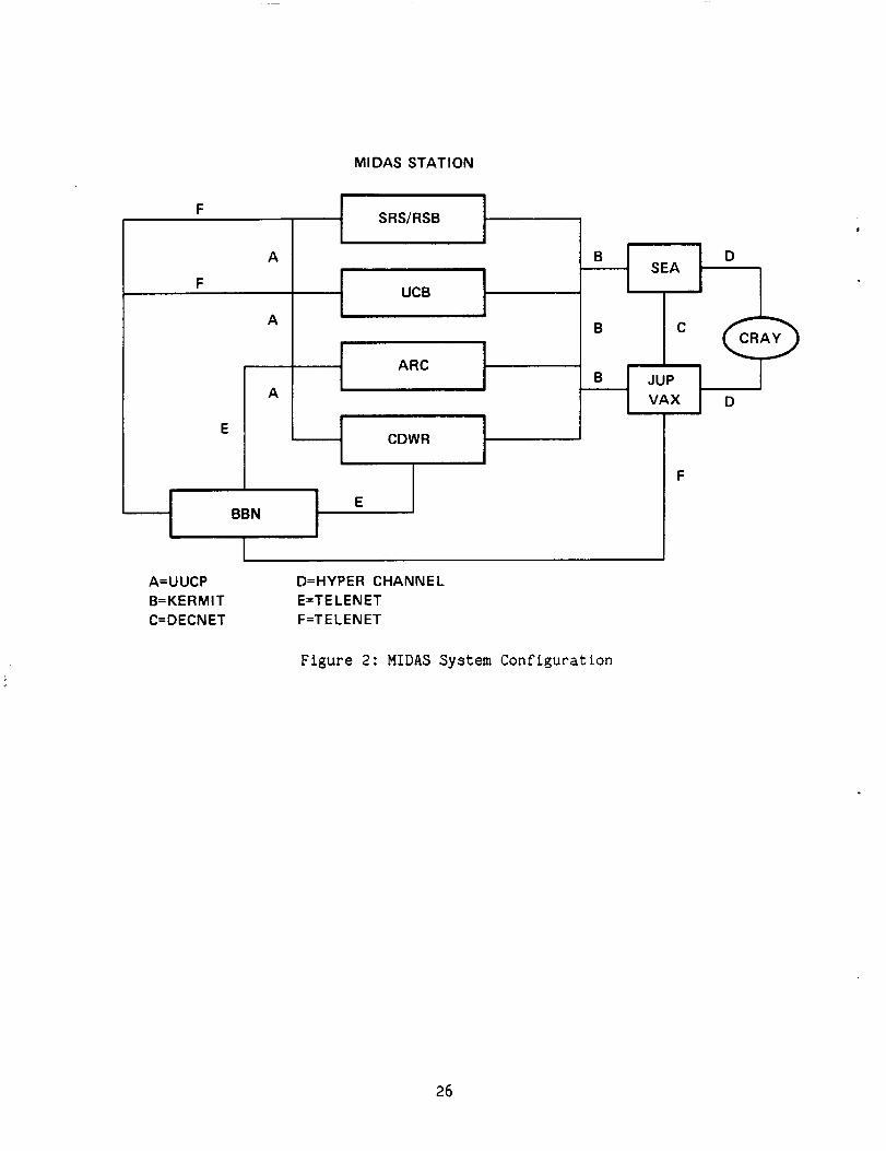
The MIDAS system configuration is shown in figure 2. Four workstations were
assembled at ARC. The ARC systems contained a MC680OO CPU board, a 1024 × 1024 × I
graphics board, 512K error-correcting multibus RAM, a disk controller board, an
ETHERNET controller board, and a 1024 × 800 black and green monitor. Each system
was equiped with an 80 MB Winchester-type disk drive except for one workstation
which has a 160 MB disk. These components allowed the workstation to function as a
microcomputer with a large amount of data storage, as required for processing geo-
graphical information. Two of the four ARC systems contained components for the
interactive display of Landsat imagery, i.e., a color frame-buffer interface board
linked to a 512 × 512 × 24 color frame buffer with pan and zoom, color lookup
tables, two graphics overlay planes, high-speed hardware vector generator, a pixel
arithmetic unit, a hardware character generator, an 11" × 11" graphics tablet and a
19" high-resolution red/green/blue color monitor (ref. 23).
Three other MIDAS workstations were assembled by A. Travlos (UCB). One each
was installed at UCB, CDWR and the Survey Research Branch of NASS in Washington.
All three were equiped were equiped with a display device, as described above, and a
16OO bpi tape drive. The workstation at UCB has a 160 MB disk.
The seven MIDAS workstations were in place by the end of 1984.
3.3.2 Workstation Communications
Communication among the MIDAS workstations is accomplished in two ways. The
MIDAS workstations at ARC are linked by ETHERNET, a high-speed, direct cable link-
age. One of the ARC workstations, designated "FOO," has access to a modem for
communication with off-site systems. All off-site MIDAS workstations have a similar
capability. The workstations at CDWR, NASS, UCB and ARC (FOO) "talk" to each other
over public phone lines using either the UUCP utility in XENIX, for electronic mail,
or Kermit, a public domain software developed at Columbia University, for file
transfer and communication, to conduct the communication.
Prior to, and during, the 1985 inventory, the MIDAS stations needed access to
BBN. Access was required for file transfer and data processing. The electronic
linkages comprising the CCRSP network are illustrated in figure I. Kermit was used
for most communications among MIDAS stations at different CCRSP sites. Arpanet, a
system maintained by the Defense Advanced Research Projects Agency (DARPA) for
communications among government and university research centers was used for most of
the communications between MIDAS and BBN (ref. 24). Arpanet supported communica-
tions between the VAX network at Ames, which includes the VAX in ECOSAT, or the VAX
network at UCB, and the BBN system in Boston. A MIDAS station at ARC or UCB could
communicate with BBN by connecting to a VAX using Kermit and then linking the VAX to
BBN using Arpanet. Some backup methods of communications, involving Telenet and
25
MI DAS STATION
I SRS/RSB
I UCB
ARC
A
F
A
A
CDWR
A=UUCP
B=KERMIT
C=DECNET
BBN t E
ID=HYPER CHANNEL
E=TELENET
F=TELENET
SEA
B C
VAX D
Figure 2: MIDAS System Configuration
26

public telephone lines, were included in the system of linkages illustrated in
figure I to provide backup access to BBN.
3.3.3 Workstation Software
MIDAS has a XENIX operating system and is equiped with three software packages
for digital data manipulation: Classified Image Editor (CIE), Earth Resources
Laboratory Applications Software (ELAS), and PEDITOR.
3.3.3.1 CIE and ELAS- CIE was written at ARC by Walt Donovan. It is a special
purpose package designed for the display and editing of single band images, espe-
cially classified images. The classified image appears as a map on a color graphics
terminal. The image may be displayed in shades of grey or in color. Color assign-
ments are made by associating a color name with a class number or numbers, or a
range of grey levels. Usually all clusters corresponding to a crop type or land use
are displayed in one color. A color key is displayed along side of the map and is
updated as color assignments are made. CIE was used by CCRSP to edit classifica-
tions before hard copies of the data were generated.
ELAS is a general purpose image-processing system developed at the National
Space Technology Laboratory. When MIDAS was brought on line, ELAS was implemented
on the new workstations by William Erickson, which was the first implementation of
ELAS on a UNIX-like operating system. ELAS includes modules for simultaneous dis-
play of up to three bands of imagery. ELAS was used by CCRSP to display Landsat MSS
bands 4, 5, and 7 so that the imagery would look similar to a high altitude, color
infrared photograph.
3.3.3.2 PEDITOR- The rationale behind the development of PEDITOR is described
in section 2.2.3. The conversion of EDITOR code to PEDITOR began in 1983 and was
completed in the fall of 1985. Most of the EDITOR code operational on the BBN
system was rewritten in Pascal. The format of the new code was chosen to make the
code as transportable as possible.
Appendix A lists the PEDITOR modules and includes a brief description of each
module's function. Approximately 80% of PEDITOR code was written, i.e. converted
from the EDITOR system, at ARC. Some modules and libraries were written at UCB and
some, such as the modules to "pack" data and perform the estimation calculations,
were written at NASS. The code was tested by NASS and ARC prior to, and during, the
inventory. The tests performed are described in section 3.3.5.
The MIDAS stations at ARC designated "FOO" was the depository for the official
version of PEDITOR. As modules, libraries, and standard reference files were com-
pleted or updated at UCB, NASS, or ARC they were transferred to FOO. The ease of
communications among the workstations made it possible to distribute PEDITOR code
electronically. In 1984, UCB assumed the responsibility to distribute PEDITOR
updates to all workstations and BBN. Upgrades or reloads involving more than one or
two modules or other files were sometimes accomplished by writing the files contain-
ing the code to magnetic tape and reading the tape at the remote sites.
27

3.4 Plan for the 1985 Inventory
A list of recommendations for the 1985 inventory was compiled by UCB, based on
the findings of the CCRSP research. These were reviewed at one of the regular CCRSP
meetings and subsequently presented to management of the CCRSP organizations and
CCLRS at the semi-annual review of CCRSP in Berkeley in September 1984. The list is
reproduced in Appendix B. A preliminary list of crops to be reported on and a
prioritization of study sites were made based on the recommendations and the inter-
ests of NASS, CCLRS and CDWR. The UCB recommendations and preliminary decisions
made at the September meeting were then reviewed in Washington by NASS. Most of the
technical recommendations made by UCB for the inventory were approved, and NASS
wrote an implementation plan for the inventory. The plan included a revised list of
crops, choice of study site, technical methodology, pro-inventory preparations, and
a work schedule.
The primary goal of the inventory was an operational test of the use of Landsat
data to develop estimates and to map major crops in California. The study site was
the Central Valley, specifically, 19 counties within the Central Valley. Acreages
estimates were to be reported for 10 major crops in Central California: alfalfa,
almonds, corn, cotton, grain (wheat and barley}, grapes, rice, deciduous
tree-fruit(citrus, olives, kiwi, etc.), tomatoes, and walnuts. These acreages were
to be reported at the regional level by January 1986, and at the county level by
March 1986o The schedule was designed to test the feasability of obtaining Landsat-
based estimates in a timely manner, i.e., in time to have an impact on the annual
acreage estimates issued by CCLRS. Map products showing the distribution of the
crops and major land-use types would be produced from the classification of the
Landsat imagery and evaluated in terms of accuracy and utility in support of CDWR
land-use inventories.
The secondary objective of the inventory was a test of MIDAS. The procedures
for the inventory were a modified version of standard EDITOR processing. A signifi-
cant difference was that most of the processing be done on MIDAS with PEDITOR. All
CCRSP participants were equiped with MIDAS stations by 1984. CDWR and NASS, espe-
cially CCLRS, appeared interested in developing the operational potential of the
workstation. In response to the presence of MIDAS and the then imminent completion
of PEDITOR, MIDAS was selected as the system of choice for the inventory. The
decision to use MIDAS was made with the understanding that BBN would be available to
assume the data processing burden should MIDAS prove inadequate for the job.
3.4.1 Technical Approach
The data processing steps involved in the Central Valley inventory are summa-
rized in figure 3. The inventory design differed from typical NASS processing in
five ways:
I. Use of three Landsat observations over the study site, rather than one or
two,
2. Use of Landsat bands 5 and 7 only from each acquisition,
28

I
A-ETHERNET CONTROLLER
B-SERIAL I/O INTERFACE
C-TAPE DRIVE CONTROL
D-2181 DISK CONTROL
E-512K RAM
F-COLOR GRAPHICS INTF
G-MC68000, 256K RAM
SERIAL I/O
H-1024 x 800 GRAPHICS
CONTROL
IEEE-796 MULTIBUS
D@
A1-ETHERNET TRANSCEIVER
B1-LINE PRINTER
C1-TAPE DRIVE
D1-80 MB DISK
B2-MODEM
D
F1-COLOR GRAPHICS CONTROL
F3-G RAPHICS TABLET
G1-KEYBOARD
HI-GRAPHICS DISPLAY
F2-COLOR MONITOR
G2-OPERATOR
CONSOLE
Figure 3: Central Valle F Inventory - Data Processing Steps
29

3. Transect ground data collection - typical processing used JES data only,
4. Map product generation - map product capabilities were included at the
request of CDWR, including detailed accuracy assessment on of the JES segments, and
5. Evaluation of the accuracy of JES survey data°
Three dates of Landsat data were to be used because the results of preparatory
research by CCRSP (section 3.2.2) indicated that three dates would yield the best
results for an inventory of California agriculture. One spring and two summer
Landsat observations would be acquired for each of the seven frames required to
cover the study site. The analysis would be done using MSS bands 5 and 7 from each
date.
Two issues related to sample allocation were addressed in the design of the
inventory. There were indications from research by NASS that bias was introduced
into the estimates when the same ground sample segments were used to train the
classifier and develop the estimates (section 3.2.2). There was concern by UCB that
the number of ground sample segments in the JES might not be adequate to sample the
spectral variation in California agriculture and was, therefore, inadequate to train
the classifier. Both issues were resolved by drawing upon the resources of CDWR to
conduct an additional survey.
In the 1983-84 growing season, CDWR conducted a systematic sample of a section
of the Sacramento Valley to determine if such a technique would sample adequately
the variation of crop types present. The survey was conducted as an independent
test, and the data collected was not used in any other task. Details of the sampl-
ing scheme are described in section 4.2.2. The survey results indicated that the
systematic sample provided sufficient data on the crop types of interest to train
the computer to recognize them in the Landsat imagery. It was decided by CCRSP to
use the CDWR survey technique to gather data for training the classifier (cluster
statistics file) and reserve the JES data for acreage estimation and accuracy
assessment.
Map products were to be generated from classified Landsat imagery because CDWR
typically delineates survey information on maps. The accuracy of Landsat classifi-
cation would be evaluated within that agency by comparison of the Landsat crop map
with other crop maps.
3.4.2 Roles of the Participating Organizations
The inventory plans called for most tasks to be completed by NASS and CDWR.
NASS, through CCLRS, was responsible for the JES data set. Preparation of the data
set included collection, tabulation and digitization of the 600 JES ground sample
segments in the study site. George May was transferred by NASS to Sacramento to
take charge of the NASS/CCLRS tasks in CCRSP. May also chaired the meetings of the
CCRSP working group and was the unofficial manager of the inventory project until
his resignation from USDA in December, 1985.
30

The primary data processing role in the inventory was taken on by CDWR.Mostof the data processing was intended for the MIDASworkstation at CDWR. That sitewas selected because becauseCDWRand CCLRSwanted an operational demonstration ofits capability, and CDWRwas commited to continuing MIDASoperations after thecompletion of the inventory. In addition to the data processing load assigned toCDWR,the agency also took on the planning, coordination, collection, tabulation,and digitization of the transect data--the training data for the Landsat classifica-tion. The ground data collected for the inventory by CDWRwas an extention of workdone by the agency for the preliminary studies reported in section 3.3.2.
The ground data collection effort for the transect data, software support, dataprocessing assistance, and technical advice was provided by UCB. Uponcompletion ofthe inventory, UCBwas to review the inventory procedures and assist with theassessmentof the quality of the crop mapsand acreage estimates generated.
AmesResearch Center was required to continue support activities, as describedin section 3.1, in particular, assistance with software, provision of U-2 photog-raphy, and execution of processing steps on the Cray X-MP. In addition, ARCwasresponsible for reformatting Landsat data tapes for processing within the EDITOR/PEDITORsystem and the development of acreage estimates following tabulation of theground survey and Landsat data.
3.4.3 Preparations
The inventory implementation plan included schedules and assignments for tasksthat needed to be addressed prior to the actual inventory. These included comple-tion and testing of PEDITOR,completion of non-PEDITORsoftware related to theinventory such as software to generate six-band Landsat data files (MSS5and MSS7from each of three dates), acquisition of current year photography of the JES seg-ments, and preparation for transect data collection.
3.4.3.1 PEDITOR testing- PEDITOR was tested by NASS and ARC. Testing by NASS
was performed at BBN with a four-channel Landsat data set. By the summer of 1985,
NASS confirmed, to the agency's satisfaction, the operation of all modules completed
at that time and declared PEDITOR operational. Additional tests were performed by
CCRSP to confirm proper function with a Landsat data set containing more than four
bands and to confirm the proper function of PEDITOR on MIDAS.
Tests of PEDITOR for CCRSP were begun by ARC in the spring of 1985. The test
data set was the 1982 Yolo County data set that had been used for the multi-crop
research described in section 3.2. The data set included an eight-channel tape of
Landsat data (MSS bands 5 and 7 from four dates) and approximately 60 JES seg-
ments. A copy of the data set was available at BBN.
The tests were performed in two stages. In the first stage, identical data was
processed through a PEDITOR module at BBN and on a MIDAS workstation at ARC. If no
run-time errors were encountered on either system, and the results were identical,
the proper operation of the module on MIDAS was confirmed. An error in the logic of
a module would produce erroneous results even though the module appeared to operate
31

correctly. Secondstage testing was done to verify the computations. Verification
was achieved by comparing the results obtained with PEDITOR on MIDAS with results
obtained using functionally similar ELAS modules or other software, and by cross-
checking the output from one PEDITOR modules.
The _nner of testing described was used to verify the correct operation of the
PEDITOR modules and MIDAS for the inventory data processing steps up to and includ-
ing classification. Testing of the estimation modules was delayed until the fall of
1985 when they were completed by NASS. By that time, the inventory was well under-
way, and the inventory data set served as the test data set.
_.4._.2 Code written for CCRSP- A limited amount of new computer code was
developed at ARC for the 1985 inventory experiment. The program COMPILE was the
most significant piece of code added. It was written to generate a 6-band tape of
MSS bands 5 and 7 from multiple registered Landsat acquisitions (section 4.1.4).
Modifications to some PEDITOR code was also required for the inventory. The
most common change was to enlarge an array because of the large number of segments
used in the survey for the training data and the large number of spectral classes
resulting from clustering three dates of Landsat imagery.
The PEDITOR modules involved in classification were installed on the ECOSAT VAX
at ARC to take advantage of the greater speed of the VAX, compared to the MIDAS
workstation, and the facilities available to submit files directly to the front-end
computer for the Cray°
3.4.3.3 Current year photography- An ARC U-2 flight in October, 1984 acquired
color infrared photography of the entire Central Valley. The photography was used
in both the JES and the transect survey. The best time to acquire photography for a
current year survey of the Central Valley is in the early spring of the survey
year. By that time, virtually all field boundaries for spring and summer plantings
have been defined. However, because of the large number of prints needed and the
need to have the prints marked with segment boundaries prior to the June survey, the
October 1984 flight data was used. It was assumed that minimal field boundary
changes would occur after the October date.
The U-2 photography was acquired as 9"x9" color transparencies. Samples from
the transparencies were enlarged, converted to color prints and submitted to CDWR
and CCRLS in Sacramento for comment. The scale and resolution of the product were
acceptable to both agencies, but CCLRS preferred the prints in black and white so
that tract and field boundaries and other enumerator marks added to the the photog-
raphy in color would not cause confusion.
Enlargements were made at ARC for approximately 300 segments. The prints were
delivered to CCLRS in early spring of 1985. They were annotated with segment bound-
aries in Washington D.C. and were used by the enumerators in the JES.
32

4. THE 1985 INVENTORY
The following account of the 1985presents a general description of events anddetails of the steps in which ARCwas a substantial contributor (Table 2). Theaccount begins with a description of the study site because geography effected muchof the work and the results obtained. Data collection, data processing, acreageestimation and mapproducts are discussed in turn. The account concludes with asummaryof system performance.
This section of the report is intended to be a comprehensive guide to the dataprocessing for the 1985 inventory. The processing was documented in the CCRSPPEDITORProcedural Manual written by CCRSPparticipants and available through UCB.
4.1 The Test Site
The test site and location of the Landsat frames which cover it are shown infigure 4. The Central Valley is the heartland of California agriculture. It is anelongated basin that stretches from the foothills of the Tehachapi Mountains southof Bakersfield north north-west approximately 400 miles to the southern extention ofthe CascadeMountains north of Redding. The width of the Valley varies between40 and 80 miles. It is boundedon the east by the Sierra NevadaMountains and onthe west by the North Coast and Central Coast Ranges. The flatness of the Valleyfloor is broken only by the Sutter Buttes north of Sacramentoand the low-lyingDunniganand MontezumaHills on the western edge of the SacramentoValley. Water isthe key to the formation of the Central Valley and to its current economic health.The floor of the Central Valley is underlain by sediments deposited in the basin bythe drainage of the San Joaquin River and its tributaries in the south and theSacramentoRiver and its tributaries in the north. Becauseof the summerdrought inthe Valley, typical of a Mediterranean climate, most agriculture is irrigated.
The Central Valley was selected as the test site because a large proportion ofthe major crops grown in California are farmed there. Over 90%of the corn, cotton,grain sorghum, and nut crops, and 100%of the rice harvested in California comefromthe Central Valley. The Central Valley was an appropriate size for the test. It issmall enough for implementation of a transect survey, and large enough to represent
a good operational test of an inventory design involving Landsat.
The diversity of crops grown in the test site affected the inventory in two
ways. First, a larger than normal sample size was required to garner adequate
training for the classifier. Second, a given crop tended to occur in a minority of
segments with many crops concentrated in a subregion of a land-use stratum within a
Landsat analysis district resulting in imprecision in expansion estimates based on
JES segments. Regression on Landsat pixels to correct the estimate of the mean
acreage per square mile could potentially lead to great improvement in the accuracy
of acreage estimates provided there was a high correlation between pixels and acre-
age and sufficient data in the JES survey to develop a regression line.
33

TABLE 2.- 1985 INVENTORY--DATA PROCESSING AT ARC
Processing stage
Landsat data preparation
Clustering
Classification/
aggregation
Estimation
Map product
generation
Function
Reformat tapes
Scene registration
Confirm registration
Map calibration
Digitized segments
Register segments
Reformat training data
Cluster
Stat file edit
Classify segments
Full frame classify
Aggregate
Regression
Large scale
Recode data
Generate maps
Job setup
M/P
M/P
M/E
M/P
M/P
M/E
M/P
M/P
M/P/E
M/P
M/P
M/P
M/P
M/P
M/E
M/E
Job execution
C/S
C/M
M/E
M/P
M/P
M/P
M/P
C/Ed
M/P/E
C/Ed
C/Ed
C/M/P
M/P
M/P
M/E
M/E
Key: M : MIDAS
Ed : EDITOR
C : CRAY
S : stand alone programs
P : PEDITOR
E = ELAS
34

/
I
I
sL_,NTA CRUZ
I,//L_._
III
L.
EL DORADO
%%
TUOLUMNE MONO_
%
OBISPO
SANTABARBARA
/
/.J
If
/!
_os/ANGELES
/
0 20 40 60 80 100|
MILES
%%
INYO
%%
\\
%%
SAN BERNARDINO,
RIVERSIDE
!
J DIEGO IMPERIAL
J ,--_i
INVENTORY COUNTIES
LANDSAT FRAME BOUNDARY
Figure 4:1985 Central Valley Inventory - Study Site and Landsat Frame Locations
35
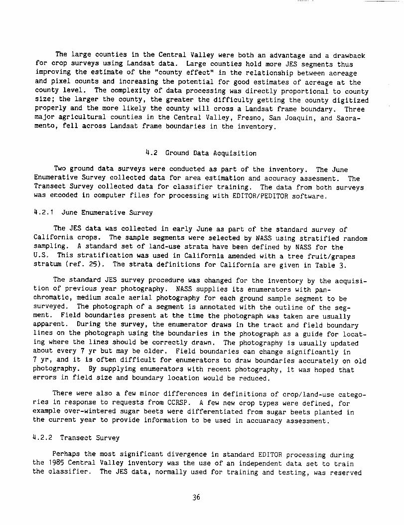
The large counties in the Central Valley were both an advantage and a drawback
for crop surveys using Landsat data. Large counties hold more JES segments thus
improving the estimate of the "county effect" in the relationship between acreage
and pixel counts and increasing the potential for good estimates of acreage at the
county level. The complexity of data processing was directly proportional to county
size; the larger the county, the greater the difficulty getting the county digitized
properly and the more likely the county will cross a Landsat frame boundary. Three
major agricultural counties in the Central Valley, Fresno, San Joaquin, and Sacra-
mento, fell across Landsat frame boundaries in the inventory.
4.2 Ground Data Acquisition
Two ground data surveys were conducted as part of the inventory. The June
Enumerative Survey collected data for area estimation and accuracy assesment. The
Transect Survey collected data for classifier training. The data from both surveys
was encoded in computer files for processing with EDITOR/PEDITOR software.
4.2.1 June Enumerative Survey
The JES data was collected in early June as part of the standard survey of
California crops. The sample segments were selected by NASS using stratified random
sampling. A standard set of land-use strata have been defined by NASS for the
U.S. This stratification was used in California amended with a tree fruit/grapes
stratum (ref. 25). The strata definitions for California are given in Table 3.
The standard JES survey procedure was changed for the inventory by the acquisi-
tion of previous year photography. NASS supplies its enumerators with pan-
chromatic, medium scale aerial photography for each ground sample segment to be
surveyed. The photograph of a segment is annotated with the outline of the seg-
ment. Field boundaries present at the time the photograph was taken are usually
apparent. During the survey, the enumerator draws in the tract and field boundary
lines on the photograph using the boundaries in the photograph as a guide for locat-
ing where the lines should be correctly drawn. The photography is usually updated
about every 7 yr but may be older. Field boundaries can change significantly in
7 yr, and it is often difficult for enumerators to draw boundaries accurately on old
photography. By supplying enumerators with recent photography, it was hoped that
errors in field size and boundary location would be reduced.
There were also a few minor differences in definitions of crop/land-use catego-
ries in response to requests from CCRSP. A few new crop types were defined, for
example over-wintered sugar beets were differentiated from sugar beets planted in
the current year to provide information to be used in accuaracy assessment.
4.2.2 Transect Survey
Perhaps the most significant divergence in standard EDITOR processing during
the 1985 Central Valley inventory was the use of an independent data set to train
the classifier. The JES data, normally used for training and testing, was reserved
36

TABLE 3.- CALIFORNIA AREA FRAME STRATA DEFINITIONS a
Stratum 13b
Stratum 17b
Stratum 19b
Stratum 20 b
Stratum 31
Stratum 32
Stratum 41
Stratum 43
Stratum 44
Stratum 45
Stratum 50
Stratum 62
Fifty percent or more cultivated, mostly general crops with less
than 10 percent fruit or vegetables.
Fifty percent or more cultivated, mostly fruit, tree nuts, or
grapes mixed with general crops.
Fifty percent or more cultivated, mostly vegetables mixed with
general crops.
Fifteen to fifty percent cultivated, extensive cropland and hay.
Agri-urban, more than 20 dwellings per square mile, residential
mixed with agriculture.
City, more than 20 dwellings per square mile, heavily
residential/commercial, virtually no agriculture.
Privately owned range, less than 15% cultivated.
Desert range, barren areas with less than 15% cultivated,
virtually no crops or livestock.
Public grazing lands, Bureau of Land Management or Forest Service
grazing allotments.
Public land not in grazing.
Nonagricultural, includes state and national forests, wildlife
refuges, military reservations, and similarly designated land.
Known water (not sampled), larger than I sq. mile.
aFrom M. L. Holko, "1982 Results of the California Cooperative Remote Sensing
Project," SRS staff report No. AGES840305, March 1982.
bMaJor crop strata--other strata not used for crop estimation in this study.
37

for estimation and accuracy assessment. A separate set of sample gound data was
collected to train the classfier. The new ground data was collected by driving
transects through the agricultural areas of interest. The data set is referred to
as the Transect Survey.
The Transect Survey was operated by CDWR, NASS and UCB personnel. Approx-
imately 2500 segments were selected and visited in mid-spring and mid-summer.
Segment selection was designed to achieve a comprehesive representation of crops and
crop conditions affecting crop appearance, as well as representation of types of
land use present in the agricultural land use strata in the California. The ground
sample units were picked through a systematic sample as follows:
I. CDWR land use maps were used to quantify crop mix on a 2.5 min block basis°
2. Areas characterized by homogenous soil color and other factors affecting
the appearance of agricultural fields on imagery were identified on 1984 Landsat
photoproducts.
3. The above information, supplemented with 1985 U-2 photography, was used to
locate transects that would maximize contact with crops of interest and sample areas
with different appearance factors.
4. The transects were drawn on road maps and assignments for the gathering of
field observations were made by county.
5. Along the transects, stops were made every 2 miles and all fields adjacent
to the stop and above a minimum size were included in the survey.
Field enumerators drew field boundaries on a map and recorded field contents,
i.e. crop type or land use. High altitude photography acquired by ARC in 1985 was
used to check the data before it was encoded.
4.2.3 Preparation of the Survey Data
The tabulated data collected by JES enumerators required key punching and entry
on magnetic tape. The task was completed by NASS. The tapes were returned to
CDWR. The ground data were loaded on MIDAS and distributed to other CCRSP sites.
The field observations collected by CDWR and UCB staff for the transect survey were
entered into computer files at CDWR interactively.
The strata network files delineating the California JES sampling frame for 16
of the 19 counties in the Central Valley test site were supplied by NASS. Strata
maps were sent to ARC for Kern, Kings and Tulare Counties. The maps were digitized
on a tablet at ARC using PEDITOR software at BBN. All 19 strata network files were
converted to mask files using PEDITOR on a MIDAS workstation at ARC.
Field boundaries were digitized into segment files at CDWR and CCLRS. The JES
segments were digitized at CCLRS. The task was made easier by the need to digitize
interior field boundaries for only the 10% sample of the JES segments that were to
be used for accuracy assessment. The transect segments were digitized at CDWR using
38

the Osborne I. As the ground data was digitized and segment network files created,the files were transferred to MIDAS,and copies were sent to BBN.
Segmentregistration is a two-step process. The first step is the generationof a calibration file for each Landsat scene relating latitude and longitude toLandsat SOMcoordinates. The calibration file is created on a digitizing tablet bylocating control points on 1:250,000 mapsand on 1:1,000,000 Landsat photoproductsobtained form EROSData Center. About 20-30 control points are needed. After thepoints are located, least squares analysis is performed on the points, and a cali-bration file is generated. The calibration files for CCRSPwere all created atCDWR.
The latitude/longitude coordinates in the segment network file are inexact dueto small errors in claibration whenthe segments are digitized. The next step inregistration corrects for the small error introduced. The calibration file is usedto identify a block of data in the Landsat scene containing the segment. A grey-scale plot of one band of Landsat data from the block containing the segment isgenerated. A plot that shows the field boundaries of the segment, drawn at the samescale as the grey-scale plot, is also produced. The second plot, a vector plot,contains tic marks that allow it to be placed correctly on the grey scale plot. Thevector plot is overlayed on the grey-scale plot and shifted until the field bound-aries in the segment plot appear to lie in the proper location in the Landsat datagray scale. The shift required for each segment is the number of pixels the segment
plot was moved, in the x and y directions, from the location predicted by the
calibration file to its proper location. The x and y shifts are recorded and
entered into a text file, with segment number, to be used for mask generation.
The intention of CCRSP was to generate all plots on MIDAS, however, the vector
plots were generated by NASS in Washington because of the unexpected length of time
required to create the plots on MIDAS. Most of the segment shifting was done at
CDWR with help from UCB and ARC. Segment registration proceeded smoothly even
though, for 90% of the JES segments, internal fields boundaries were not available
to match the vector and grey scale plots. Upon completion of segment shifting, mask
files were created using the appropriate calibration file, segment network file and
file of segment shifts. All segment mask generation for the inventory was done at
CDWR.
4.3 Landsat Data Preparation
Acquisition and preparation of the Landsat data started at about the same time
in the spring as ground data collection but wasn't completed until the end of Oct-
ober 1985. Because of the quantity of data that had to be manipulated, and the need
to store the data on tape, all Landsat data preparation was done at ARC.
4.3.1 Landsat Data Acquisition
The Landsat data was ordered by NASS. The EROS catalogue containing the scene
information was checked regularly as the time window for acquisitions was entered.
39

The window extended from March through September. The intent was to obtain a spring
acquisition, an early summer acquisition, and a late summer acquisition for each of
the seven frames required for the inventory. Within that window, acquisitions were
selected to maximize data quality and minimize percent cloud cover. Data was
ordered as computer compatible tape and 1:1,000,000 black and white prints. The
tapes were the primary data source. The prints were needed for the preliminary work
in scene-to-scene registration and for general reference.
The frames came from three Landsat paths. The acquisitions selected are listed
in Table 4. The worst cloud problem was in frame path 44, row 33 where part of
Sacramento County between the cities of Sacramento and Lodi was obscured by cloud or
cloud shadow on the 5 May 85 acquisition. Some patchy clouds were also unavoidable
on path 42.
The data tapes were sent to CCLRS first and forwarded to ARC for processing.
The first two acquisitions for each of the seven frames was received at ARC by early
August. The last acquisition was received by early October.
4.3.2 Reformatting of Landsat Scenes
The Landsat digital data arrived from CCLRS in EROS band interleaved (BIL)
format on 6250 bpi tapes. The data left ARC reformatted into six-band data sets in
the two formats described in section 2.2.2oi and suitable for processing at BBN or
on a MIDAS workstation.
The first step in preparation of the data was to reformat the EROS raw data
tapes so that the data would be compatible with the registration software on the
Cray. The second step was to register the data. Before the scenes could be regis-
tered, a base date had to be selected.
The second acquisition in each frame was chosen as the base (primary) date,
i.e., the Landsat SOM coordinates on the second date were chosen as the coordinates
for the six-band data sets.
The reformatted data was registered using the block correlation technique
(ref. 7). The initial overlay was performed at CDWR. ARC took advantage of the
automated block editing in the latest version of BCORR to eliminate manual editing
of the correlation blocks. Sample sections were extracted and displayed from each
pair of registered scenes to verify that the registration was correct.
The third acquisition of all frames was received at ARC in late September. By
early October, the scenes were registered to the primary dates, and all frames were
ready for the final processing step, creation of the six-band data set.
The program COMPILE created the new tapes. The frames were split into an
eastern and western half so that no tape file contained more than 1950 columns.
There was a 100-column overlap between the halves. Splitting the data was necessary
because BBN could not read records longer than 20,000 bytes, and MIDAS could not
read a tape file that extended beyond a single reel of tape. The COMPILE program
40

TABLE 4.- LANDSAT ACQUISITIONS FOR 1985
CENTRAL VALLEY INVENTORY
Path/row
(frame)
42/35
42/36
43/34
43/35
44/32
44/33
44/34
Acquisition date
20 MAR 85
2 JUL 85
12 SEP 85
20 MAR 85
2 JUL 85
12 SEP 85
14 MAY 85
17 JUL 85
18 AUG 85
14 MAY 85
17 JUL 85
18 AUG 85
5 MAY 85
8 JUL 85
25 AUG 85
5 MAY 85
8 JUL 85
25 AUG 85
5 MAY 85
8 JUL 85
25 AUG 85
Scene ID
50384-18043
41082-17582
50560-18032
50384-18045
41082-17585
50560-18034
50439-18100
50503-18094
50535-18093
50439-18102
50503-18101
50535-18095
50430-18152
50494-18151
50542-18144
50430-18154
50494-18153
50542-18151
50430-18161
50494-18160
50542-18153
41

read the three registered scenes for a frame, extracted MSS bands 5 and 7 from each
half scene, and wrote a new six-band tape in BBN format at 1600 bpi. BBN format
(pixel interleaved, 664 byte header) was chosen so that the data set would be com-
patible with BBN and MIDAS.
4.3.3 Formatting Landsat Coverage of Segment Data
The Landsat coverage of the JES and Transect Survey segments was processed to
form compact data files by packing portions of data from the half scene tapes. In
the standard EDITOR procedure (section 2.2.2.1), one packed file is created for each
crop/land-use type within a Landsat analysis district (Landsat path°) The inven-
tory, however, generated multiple packed files for each crop/land-use type because
of the large number of training segments and a 300 segment limit on the number of
segments in a packed file. Two packed files were required for each crop/land-type
use in two of the analysis districts, and three packed files were required in the
third.
CDWR intended to create all the packed files in Sacramento but was precluded
from doing so by the slow speed of the MIDAS station and the propensity for the
system to crash if more than five crop/land-use types were packed at one time.
Because of the interest in completing the estimates on schedule, some of the packed
files were created at UCB and ARC.
4.4 Landsat Data Processing and Interpretation
Maximum likelihood classification was performed to label each pixel in the six-
band data sets with a crop type or land-use category. The data was clustered first
to estimate the distribution parameters for the crop/land-use types. Following
classification, pixel counts on JES segments were tabulated, and the tabulations
were used to compute crop acreage estimates and to gauge the accuracy of the classi-
ficationo
4.4.1 Training for Classification
The classifier for each analysis district was trained to recognize crops and
land-use types by clustering the brightness data contained in the sample segments of
the Transect Survey. Virtually all clustering for the inventory was done with the
CLASSY algorithm on the Cray X-MP at ARC. The intent of the inventory was to set up
and submit the CLASSY jobs from CDWR. As in packing, however, the press of time
forced a change in plans. The files packed at UCB and CDWR were sent to ARC where
the clustering jobs were set up and submitted.
Job set up for clustering was accomplished using a PEDITOR module on the SEA
VAX. The module, CRAY, automatically formats Cray Job control language when the
user identifies the type of job to run and other parameters required for the partic-
ular Job type. The output from the CRAY module is a text file that can be submitted
directly to the Cray, via DECNET, from the SEA VAX. Multiple-packed files were
submitted in a single job, but each file was clustered individually.
42

The output from the CLASSYprogram was a text file containing the statistical
information on the data clustered. The output file was returned automatically to
the SEA VAX. The CRAY module was used, again, to reformat the data in the output
file. After reformatting, every crop/land-use type clustered had a separate statis-
tics file in PEDITOR format. The statistics files were written to tape and mailed
back to CDWR or UCB as appropriate, for the next step in processing, editing the
statistics files.
4.4.2 Statistics File Editing
The statistics files for each Landsat analysis district were combined and
edited. Editing was required because, for all analysis districts, the number of
clusters in the combined statistics file exceeded 255, the maximum number of
clusters the classifier could process. Editing was also advisable because of the
following:
I. Some clusters were associated with a small number of data points. The
significance of these clusters and the stability of the statistics, particularly the
covariance matrices, were thus in doubt.
2. Improvements in the quality of the classifications might result from cor-
recting for imperfections in the training data. The transect data might have con-
tained a few errors, undetected mistakes in the deliniation of fields or in record-
ing of crop/land-use type. Some fields could be atypical or highly variable in
appearance.
3. In a few cases, the training data was drawn from areas near an edge of the
Landsat path, with no valid reflectance data on one or more observation dates.
These points had values of 255 on some channels.
The stategy for editing clusters was agreed upon after several discussions at
CCRSP meetings. Responsibility for this work was split among members. Path 42 was
assigned to CDWR and USDA, Path 43 to ARC, and Path 44 to UCB. The task required
some descretion, but the following criteria were used by all cluster editors to
remove clusters:
I. Clusters with less than 100 points,
2. Clusters with three or more channels with very high variance (17 or more
grey levels in the standard deviation in brightness detected by the Landsat
scanner),
3. Clusters with a mean of 255 in one or more channels, indicating invalid
Landsat data,
4. Clusters that were similar to a large number of other clusters.
The clusters were removed in the order shown above. In the last step, the
Swain-Fu distance (refs. 11,26) was calculated for all cluster pairs and was the
criterion for removing clusters. The Swain-Fu distance measures spectral
43

similarity, or degree of overlap, between two clusters using a formula which normal-
izes the ordinary Euclidean distance between cluster means by a factor related to
the cluster shapes and volumes, as indicated by the cluster statistics. Clusters
that were less than 0.6 in Swain-Fu distance from more than 20 other clusters were
scrutinized carefully. Some clusters were similar to 50 or 60 other clusters. Most
of similar cluster pairs were of the same crop/land-use type. Clusters that were
similar to clusters associated with dissimilar crop/land-use types, that is, areas
in the transect segments that should have looked different on the Landsat data on
one or more of the three observation dates, were the first to be eliminated. The
final statistics files for paths 42, 43, and 44 contained 223, 169, and 231 clusters
repectively.
4.4.3 Classification and Aggregation
The classification job control files were created on the ECOSAT Vax with PEDI-
TOR software, and the Landsat data were classified on the Cray at ARC. Two classi-
fications were performed per analysis district. The same classifier, i.e. the same
cluster statistics file, was used for both classifications. A "small-scale" classi-
fication was performed first on packed JES segments and "large-scale" classification
on the half-scene tapes. "Large-scale" classification and aggregation, tabulation
of pixel counts by crop/land-use label and stratum, were performed sequentially as
two parts of the same Cray job.
Aggregation requires mask files of the strata. The program will abort if the
strata mask window extends beyond any edge of the classification. Because most
strata mask files extend across Landsat image boundaries, the mask files must be
edited, i.e., split along frame boundaries before use in aggregation. That type of
mask splitting is a standard EDITOR processing step, and the strata mask files for
the 1985 inventory were split in that manner. However, additional editing of the
strata mask files was required for the 1985 inventory, because several of the frames
were split into two halves as described in section 4.3.2.
Strata mask-file editing for CCRSP was accomplished at ARC the week of 9 Decem-
ber 1985. Personnel from CDWR came to ARC to complete the processing. The masks
were edited to exclude the parts of each frame that were outside the three-date
overlap zone, and split to accomodate masks that crossed analysis district bound-
aries. Some of the processing was done on MIDAS. Errors in the software, and the
slowness of the system compelled the analysts to perform some operations at BBN.
Following completion of the strata mask editing, large-scale classification and
aggregation proceeded. Each half frame was classified with the appropriate statis-
tics file and the labelled pixels were aggregated with the strata mask files. The
data processing was done on the Cray with job set-up on the SEA VAX. The outputs
from the Job were a tape of the half-frame classification and a text file of the
pixel counts by crop/land-use type and stratum aggregations. The tape was stored
for later copying and distribution to CCRSP participants. The text file was refor-
matted using the CRAY module in PEDITOR. The text file was split, by county, into
individual aggregation files and each file was written to disk in PEDITOR format.
Each aggregation file contained a tabulation, by class and stratum, of the pixels
44

classified within the area delineated by the mask, a county or portion of a countywithin a half scene. The aggregation files were used in estimation.
4.5 Estimation
Several techniques were used to include Landsat pixels in the computation ofacreage estimates. The primary techniques were those developed in EDITORanddescribed in section 2.2.2.3. Those techniques were used to generate the estimatesreported for deadlines established in inventory plan (section 3.4) and for revisionsmadeat a later date. Additionally, two experimental procedures were tested - ratioestimation (ref. 4, Chapter 6) and robust regression (ref. 18, Chapter 5).
Most of the data processing for estimation was performed on a MIDASworkstationat ARCusing PEDITORsoftware. The county estimates were generated using the EDITORprograms at BBNbecause they had not been included in PEDITOR,and therefore werenot available on MIDAS. Files were transfered to and from BBNusing Kermit betweenSEAVAXand MIDASstations at ARC,and FTPbetween the SEAVAXand BBN.
Personnel at ARCrelied upon NASSstaff, in particular Martin Ozgaand MaryanneCummins,for guidance during the data processing for estimation because of ARC'slack of experience with someof the modules, and the tendency for features andperformance of the software to change from year to year. The procedures were docu-mented as they were used in the work reported here.
Experimental estimates were generated on the ECOSATVAX. Programs in theBiomedical Data Programs (BMDPStatistical Software, Department of Biomathematics,University of California, Los Angeles) were used to examine the frequency of occur-rence of selected crops in the agricultural strata and for computation for ratioestimates. A Fortran program, using a subroutine from the IMSL Library (Interna-tional Mathematical and Statistical Libraries, Inc., Houston, Texas) was used fordevelopment of robust regression estimates with inventory data and for testing theperformance of the robust procedure with simulated data, as described in Appendix C.
4.5.1 The Original Landsat Estimates
Standard EDITOR/PEDITORprocedures were followed to develop estimates describedin section 2.2.2.3. Two decisions were madeby the analyst. The first decision wasselection of land-use stata to be included in the estimates. As indicated inTable 5, the most important land-use strata were 13, 17, and 19. Stratum 20 wasincluded for grain acreage. The second decision was the choice of type of estimatorfor each stratum (within an analysis district)--regression with Landsat data orproration with JESdata only. Proration was used for strata without sufficient JESdata for development of a regression line, or in cases where the regression lineseemed"unreasonable." An ideal regression line would have a zero Y-axis interceptand a slope of 0.8. As can be seen in Tables 6A-6C, manyof the regression lineswere very different from the ideal. It was not clear whether the variance inregression line parameters was the result of consistant patterns of omission orcommission in the classifications of Landsat or the result of other factors such as
45

TABLE 5.- 1985 CALIFORNIA JES AREA FRAME POPULATION (N)a
AND SAMPLE (m)b SIZES
Stratum
13
17
19
2O
31
32
41
43
44
45
5o
62
AD42
N/m
2095/67
AD43
N/m
956/25
AD44
N/m
2336/73
ADDE c
N/m
385/23
1637/61
49/I
604/15
O/I
O/0
O/3
o/0
o/0
0/0
o/o
o/0
1898180
1510/37
332/8
O/2
0/O
O/2
0/0
o/0
0/O
o/o
o/0
917/40
606/7
607/13
O/2
0/2
O/2
O/O
0/0
45/0
O/0
O/O
o/1399/13
64/50/2
o/1o/14o/o
o/5o/1o/1
o/o
asize in # segments as represented in the frame unit
file developed by CCRSP. Strata with little acreage in
agriculture were not included.
bsize in # segments in the JES sample used in develop-
ment of regression lines, except for analysis district
ADDE.
CAn artificial district. In the frame unit file, N
represents size of regions in paths 43 and 44 covered
by cluds or smoke on the date of one or more Landsat
passes. In the segment catalogue file, m represents
segments listed as located in ADDE because of cloud or
smoke cover, data processing problems, or outside of
Landsat coverage (Kern County).
46
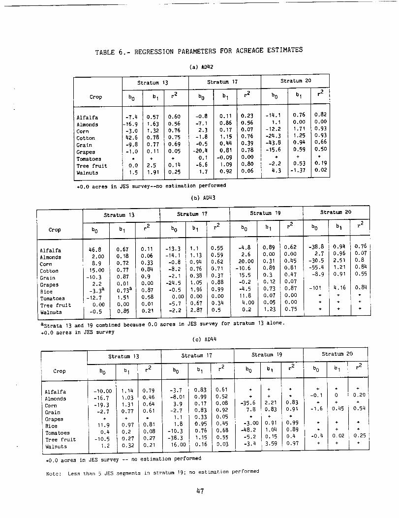
TABLE 6.- REGRESSION PARAMETERS FOR ACREAGE ESTIMATES
(a) AD42
Stratum 13
Crop
Alfalfa
Almonds
Corn
Cotton
Grain
Grapes
Tomatoes
Tree fruit
Walnuts
b0 b I r2
-7.4 O.57 O.60
-16.9 1.63 0.56
-3.O 1.32 0.76
42.6 0.78 0.75
-9.8 0.77 0.69
-1.0 0.11 0.05
0.0 2.5 0.14
1.5 1.91 0,25
Stratum 17
b0 b1 r 2
-0.8 O. 11 0.23
-7.1 O. 86 O. 562.3 O. 17 0.07
-1.8 1.15 0.76
-O.5 0.44 0.39-20.4 0.81 0.78
O. 1 -0.09 O.O0
-6.6 1 .O9 0.801.7 0.92 0.06
Stratum 20
b0 b 1
-14.1
1.1-12,2
-24.3
-43.8
-15.6
÷
-2.2
_.3
0.76
0.00
1.71
1.25
0.940.59
+
0.53I-I .37
+O.O acres in JES survey--no estimation performed
(b) AD43
r 2
0.82
0.00
O.93
0.93
0.66
0.50
+
O.19
0.02
Crop
Stratum 13
b 0 b 1 r 2
Alfalfa 46.8 0.67 0.11
Almonds 2.00 0.18 0.06
Corn 8.9 0.72 0.33
Cotton 15.00 0.77 0.84
Grain -10.3 0.87 0.9
Grapes 2.2 0.01 0.00Rice -3.3a 0.73a 0.87
Tomatoes -12.7 1.51 0.58
Tree fruit 0.00 0.00 O.01
Walnuts -0.5 0.85 0.21
Stratum 17
bO b 1 r 2
-13.3 1.1 0.55
-14.1 1.13 0.59
-0.8 0.94 0.62
-8.2 0.76 O.71
-2.1 0.38 O.37
-24.5 1.05 0.88
-0.5 1.96 0.99
0.00 0.00 0.00
-5.7 0.67 0.34
-2.2 2.87 0.5
astrata 13 and 19 combined because 0.0 acres
+O.O acres in JES survey
Stratum 19
b 0 b 1 r 2
-4.8 0.89 0.62
2.6 0.00 0.00
20.00 0.31 0.45
-10.6 0.89 0.8115.5 0.3 0,47
-0.2 O. 12 0.07
-4.5 0.73 0.87
11.8 0.07 0.004.00 0.05 0.00
0.2 1.23 0.75
in JES survey for stratum 13 alone.
(e) AD44
Stratum 20
b0 bI r2
-38.8 0.94 0.76
2.7 0.96 0.O7
-30.5 2.51 O.8
-55.4 1.21 0.84
-8.9 0.91 0.55
-101 4.16 0.84
÷ ÷ +
÷ ÷ ÷
Stratum t3
Crop
Alfalfa
Almonds
Corn
Grain
GrapesRice
Tomatoes
Tree fruit
Walnuts
b 0 b 1 r 2
-10.00 1.14 0.79-16.7 I .03 0.46
-19.3 1.31 0.64-2.7 0.77 O.61
11.9 0.97 0.81
0.4 0,2 0,08
-10.5 0.27 0.27
1.2 0.32 0.21
Stratum 17
b 3 b 1 r 2
-3.7 0.83 0.61
-8.01 0.99 0.52
3.9 0.17 0.08
-2.7 0.83 0.92
I.I O.33 o.o5
1.8 0.95 0.45
-10.3 0.76 0.68
-38.3 1.15 0.5516.00 0.16 0.03
Stratum 19
b0 b 1 r 2
Stratum 20
b0 b 1 r 2
+ + + + + +
÷ ÷ + -0.1 0 0.20
-35.6 2.21 0.83 + + +7.8 0.83 0.91 -1.6 0.45 0.54
+ + +
-3.00 O.91 0.99 ÷ + +
-48.2 1.O4 0.89 + + +
-5.2 0.15 0.4 -0.4 0,02 0.25-3.4 3.59 0.97 + + +
+0.0 acres in dES survey -- no estimation performed
Note: Less than 5 JES segments in stratum 19; no estimation performed
47
insufficient sampling or outliers, i.e., atypical segments. Large values of R2 in
some cases were an indication that the former hypothesis was sometimes correct.
Further analysis and investigation was not possible due to time constraints, there-
fore the rather conservative decision was made to use proration (direct expansion)
if the regression line slope was less than 0.5 or greater than 1.5. Estimates for
tomatoes, walnuts, and, in some analysis districts, corn, rice, and almonds were
largely based on proration.
Acreages in cloud- or smoke-obscured areas in Fresno and Sacramento Counties
were estimated by proration on JES data alone. The cloud-obscured areas were iden-
tified by defining a cloud stratum and using it in addition to the land-use strata
defined for the JES.
Estimates of the crops by analysis district were developed using both MIDAS/
PEDITOR and BBN/USDA-EDITOR. All modules for the computations involved had been
installed and tested on MIDAS/PEDITOR, but some modules could be executed on the BBN
system more rapidly. The BBN system was therefore used for some steps in the proce-
dure in order to save time. The analysis district estimates were reported in
January 1986. As mentioned earlier, county estimates were developed at BBN, and
these were reported in early March.
All estimates were reviewed with Ron Radenz of the CCLRS, and by other CCLRS
staff members. The table of Landsat estimates for a crop included, for each of the
19 counties in the test site, the estimate of total acreage and of root mean square
error (RMSE) and a breakdown of the numbers by method of estimation, regression and
proration. The Landsat estimates of acreages by county were compared with 1985
preliminary planted and preliminary harvested acreages developed at the CCLRS for
corn, wheat, rice, and cotton, and with acreage estimates for grapes, almonds, and
walnuts listed in 1984 California Fruit and Nut Acreage (ref. 27). The quality of
the Landsat estimates was also judged by examining the RMSE included in the tables
created by PEDITOR. It was noted that there was good agreement between the Landsat
estimates and the CCLRS numbers in many cases, but considerable disagreement in
others. Several major cases of disagreement occurred for crop estimates for Kern
and Tulare Counties in the southern part of the Central Valley, where the differ-
ences between the Landsat acreages and the CCLRS acreages were several RMSE's. The
Landsat estimate of rice in Merced County was only about a tenth that reported by
the CCLRS and several RMSEs below the CCLRS number.
Other cases of disagreement occurred when the Landsat estimate was primarily
based on proration, that is, when the prorated part of the acreage estimate was
larger than the regression part. Estimates involving a large component from prora-
tion had large estimates of RMSE. This was because the difference between crop
prevalence in a county/stratum and crop prevalence in the stratum as a whole was not
accounted for in the prorated acreage estimate, because there usually only a few and
sometimes no JES segments in a county/stratum for estimating this difference. There
was, however, sufficient data to estimate the variation in crop prevalence among
counties, and this was included in the estimate of RMSE. The Landsat acreages
therefore tended to be inaccurate as shown by comparison with CCRLS acreages, but in
general, estimates of precision for these estimates were accurate, i.e., the
48

magnitude of the difference between the Landsat estimate and the CCLRSacreage wasthe same or smaller than the RMSE.
The regression part of the total county estimate was negative in a few cases,
due to a negative intercept in the regression line and a small number of pixels for
the crop. This anomaly was a possible contributor to underestimated acreages such
as that for Merced rice and lead to a negative estimate for the rice acreage in
Solano County {compared to a report of zero acres in the CCRLS report).
The conclusion of the meeting with Radenz was that while some of the estimates
looked good and the inclusion of RFLSE's for the estimates was a potentially useful
feature of the Landsat acreage report, the cases of inaccuracy were a problem. It
was agreed that these problems would be investigated so that they could be
understood and perhaps rectified. The emphasis was to be on cotton, rice, and
grapes, because CCRLS had confidence in its acreage reports for these crops and the
accuracy of Landsat estimates could be assessed. The CCLRS estimates for grapes
were particularly accurate because a special survey had been made the previous year
(ref. 28).
4.5.2 Revised Estimates
The problems noted above with some of the estimates were addressed at ARC by
reworking the county estimates using the original input data, because it was judged
that some of the problems were due to ineffective estimation techniques. The Land-
sat classification in Merced County was viewed on the MIDAS system color monitor
using ELAS software. Pixels which had been labelled rice were concentrated in areas
known to be the primary rice-growing region in the county. There were 6547 rice
pixels, equivalent to over 5,000 acres in terms of the area represented by these
pixels, which was much closer to the CCLRS figure {10,100 acres) than the original
Landsat estimate (1063 acres). The classification was therefore Judged to be gen-
erally accurate in delineation of rice fields, and that the problem with the
estimate was not due to bad data. As noted above, other estimates derived primarily
by proration or involving regression with a negative intercept tended to be inaccu-
rate, suggesting that changes in estimation technique might lead to better results.
Some revisions to the original county estimates reported in early March were
made. Experimental estimation techniques were tested and will be described below.
These were restricted to Paths 43 and 44, because of concern about the quality of
data, in particular potential problems in the classified Landsat imagery caused by
procedural errors in Path 42. Much of the Landsat data analysis had been reviewed
by CDWR and UCB as part of the accuracy assessment task summarized in section 6. A
review of the cluster statistics file for path 42 indicated that some clusters might
have been mislabeled, that is, associated with crop different than that reported in
the JES survey for fields with the pixels used for development of cluster statis-
tics. Some problems were noted with data for Paths 43 and 44, but these were
judged, at least by ARC personnel, to be minor in effect, and the all the new
estimates described in this report were based on the same data as the original
estimates.
49

A few experiments were conducted in order to discover the best rules for deci-
sions in construction of a revised set of county estimates. New estimates were
created only for counties in Paths 43 and 44, because of concern over the effect of
analyst error in classification of Path 42, and only for crops for which CCLRS
acreages were available, so that the quality of the results could be judged. New
estimates were created, wherein pixel counts for the major agricultural areas,
strata 13, 17, and 19, were always included in computations. To ensure that there
were a sufficient number of JES segments to develop the regression equations, strata
were grouped. The grouping was based on CDWR's judgement from familiarity with the
geography of the Central Valley and with the JES data, and on measurements of crop
frequencies in segments within strata. Strata 13 and 19 were similar to one another
in terms of physical geography and crop mixes and were therefore grouped to form a
new combined stratum. Stratum 17 was always included in the estimates separately
because the crop mix, dominated by vines and orchards, was distinctive. Stratum 20,
when included in an estimate, was also kept separate, as it was primarily rangeland.
Ratio estimates (see section 4.5.3) were developed for walnuts and rice to
explore both the effect of including Landsat data from additional strata and of
eliminating the possibility of a negative intercept in the regression line. Regres-
sion estimates for these crops were also made on the grouped strata. The results
are shown in Table 7. The ratio estimates were similar to regression estimates.
The new rice estimates were somewhat better than the original estimates, except that
the new estimates for rice in San Joaquin County, where the quality of the classifi-
cation might have been effected by a few thin clouds on the July acquisition of
Landsat imagery, were much higher than the CCRLS estimate. The new walnut estimates
were much closer to those in the 1984 Fruit and Nut Report than the estimates com-
pleted earlier were, because stratum 17 was prorated in the original estimates
making the estimates depended on the prevalence of walnuts in the JES segments.
Ratio or regression estimates made a major difference because the prevalence of
walnuts, as indicated by pixel counts, was much higher in stratum 17 as a whole than
in the JES segments.
The results of the experiments with walnuts and rice indicated that better
estimates for other crops might be obtained by using regression instead of proration
wherever possible, that is, on grouped strata with sufficient numbers of segments.
New regression estimates were made rather than ratio estimates because of more
developed software and because a good estimator for the variance of ratio estimates
at the county level had not been developed. If the estimate of acreage within a
stratum was negative, it was replaced with an estimate of zero.
In keeping with the philosophy of maximal use of Landsat pixel counts, the use
of stratum 20 was reexamined. Although stratum 20 contains mostly native vegeta-
tion, pasture, and grain fields in hilly areas in the Central Valley, other crops
were grown there in the 1985 growing season. Personnel involved in the CCRSP had
noted almond orchards in some upland areas in the Central Valley during an observa-
tional tour of crops in the area. The statewide estimates of corn, grapes, almonds,
and walnuts in the JES report [George May, personal communication] indicated that
more than 5% of these crops were grown in stratum 20. Estimates were generated for
5O

TABLE 7.- COMPARISON OF SEVERAL TYPES OF LANDSAT ESTIMATES
FOR RICE AND WALNUTS WITH CCLRS ESTIMATES
Landsat Estimates CCLRS(4)
Ist est. (I) 2nd est. (2) I ratio est. (3) PHV
Rice Acreage Estimates for Counties in Landsat Pathes 43 and 44
Butte
Colusa
Contra Costa
Glenn
Madera
Merced
Placer
San Joaquin
Solano
Stanlslaus
Sutter
Tehama
Yolo
Yuba
14 County Total
73897
114465
67883
1400
I063
5129
30890
1797
77922
1435
17261
26155
391496
73868
1135991645
678230
49634511
100340
0779201420
20081
245314OO395
76954
113262
654
692O9393
55283350
92051888
95760262
133328683
23523395201
72000
97000
68000
200
11000
4000
4000
2500
72000
1600
2500027OO0
384300
Walnut Acreage Estimates for Counties in Landsat Pathes 43 and 44
Butte
Colusa
Contra Costa
Glenn
Madera
Merced
Placer
San JoaquinSolano
Stanislaus
Sutter
Tehama
Yolo
Yuba
14 County Total
31842683
8743146
4102
6737613
11810
155775342628
23OO
2854
1360
51382
535252401616
31752514
8496242
310381472
35658
55933326
34111877
109010
129872607
494
6856
235412740
332
228341614
26419
628510488
29744532
1133516
148794593
455251401822
8662
94428568
310224770
1395711242
6714
5744
134689
(I)
(2)
(3)
The preliminary estimate using Landsat data, reported in March 1986, Fuller-
Battese regression on Landsat on some strata, proration on other strata.
Using Landsat, Fuller Battese regression on all land use strata with
agriculture achieved by defining the regression line slope and intercepts on
grouped strata; one group was general crops strata (13, 19), the othergroup -- the tree crop stratum (17).
Using ratio estimation (as in Cochran, Sampling Techniques), with the ratio
multiplier defined for the grouped strata used in the 2nd estimate.
(4) Preliminary Planted Acreage from CCLRS, see Note I for Table 8C.
51

these crops both without and, in cases where there were at least two JES pixels with
acreage in the crop of interest, with stratum 20. Inclusion of stratum 20 improved
estimates of almonds and corn. There were not sufficient JES data to include
stratum 20 for walnuts and grapes. Visual examination and review of pixel counts in
stratum 20 revealed a very significant problem with errors of commission in the
discrimination of grapes on the Landsat imagery so that a good estimate of grape
acreage in this stratum with Landsat data might not have been possible even if more
JES data were available.
For most crops, the new regression estimates were very similar to the original
estimates. The original estimates were, therefore, reported at the final CCRSP
review and are shown in Table 8. As expected, the estimates for walnut acreage were
much higher than in the original estimates. The newer estimates for grapes in
analysis district 44, rice in stratum 43, and tomatoes in analysis district 44 were
closer to CCLRS estimates. These estimates are shown in Table 8.
The best estimates for a given crop were the estimates which included the use
of Landsat data to estimate acreage in the most important stratum for the crop, and
the estimates selected for Tables 8A-8H conform to this rule. Estimates for grapes
and tree crops included regression on Landsat pixels in stratum 17. The best
estimates for field and row crops included regression on stratum 13, or on strata 13
and 19 combined.
4.5.3 Experimental Estimates
The ratio estimate was tested on two crops, rice and walnuts, because the small
number of fields in the JES containing these crops led to regression lines with
negative intercepts, and sometimes negative county estimates. The estimate of the
county mean was of the form:
Est(Yc, h) = R × Xc,h(5)
with:
R : yh/Xh(6)
In cases where there was insufficient data for regression, or development of a
ratio estimate, strata were pooled as stated in the previous section. The results,
shown in Table 7, were similar to those achieved by regression on the same stratum
groups, as shown by examination of Tables 8A-SH and discussed in the sec-
tion 4.5.2. The sum of acreage estimates for all the counties within analysis
districts 43 and 44 were closer to the sum of CCRLS estimates when the ratio estima-
tor was used.
Some experiments with a robust regression estimator were carried out. The
ordinary least squares (OLS) regression line is often strongly affected by a few
outlier points. In agricultural inventories that use Landsat, outliers may have
occurred due to errors in JES information or to some condition in a field, such as
infestation with weeds or disease, that leads to an atypical spectral response in
52

TABLE 8A.- LANDSAT ACREAGE ESTIMATES:
ALFALFA
Estimation technique by Landsat path:
P42--s/re a for strata 12,20; prb for stratum 17
P43--s/re for strata 13, 17, 19, 20
P44--s/re for strata 13, 17; pr for strata 19, 20
County
Butte
Colusa
Contra Costa
Fresno
Glenn
Kern
Kings
Madera
Merced
Placer
Sacramento
San Joaquin
Solano
Stanislaus
Sutter
Tehama
Tulare
Yolo
Yuba
Estimate
3246
7908
82386
21401
65320
36281
33797
79036
Standard
error
1944
2922
13795
2374
10448
8820
9723
10422
9639
10247
58566
8O48
60O92
3704
49O5
52760
16144
2229
5059
1568
6964
1282
8892
1661
607
6114
2636
813
aLeast squares regression on a single
variable
bproration on JES survey data (Landsat
not used)
53

TABLE 8B.- LANDSAT AND CCLRS ACREAGE ESTIMATES:
ALMONDS
Estimation technique by Landsat path:
P42--s/re a for stratum 17; prb for strata 13, 19, 20
P43--s/re for strata 17, 20; pr for strata 13, 19
P44--s/re for strata 13, 17; pr for strata 19, 20
County
Butte
Colusa
Contra Costa
Fresno
Glenn
Kern
Kings
Madera
Merced
Placer
Sacramento
San Joaquin
Solano
Stanislaus
Landsat
Estimate
41050
6981
36023
13899
34003
16670
30360
65829
630
588138671
1565
62996
Standard
error
4471
3659
7828
3440
8453
11132
15821
12259
12272
3430
4824
1746
175O8
Sutter
Tehama
Tulare
Yolo
Yuba
6599
10404
37135
7586
5839
2812
2OO37601
3734
1613
CCLRS e
38820
14055
2267
31204
12333
83926
4922
33174
65854
152
23
37631
2900
64545
4973
7627
11187
10184
1823
aLeast squares regression on a single variable
bproration on JES survey data (Landsat not used)
CEstimates from L. O. Larson, L. S. Williams, and
S. Severson, California Fruit and Nut Acreage,
California Crop and Livestock Reporting Service,
July, 1985.
54

TABLE 8C.- LANDSAT AND CCLRS ACREAGE ESTIMATES:
CORN
Estimation technique by Landsat path:
P42--s/re a for stratum 13; prb for strata 17, 19, 20
P43--s/re for strata 13, 17; pr for strata 19, 20
P44--s/re for strata 13; pr for strata 17, 19, 20
County
Butte
Colusa
Contra Costa
Fresno
Glenn
Kern
Kings
Madera
Merced
Placer
Sacramento
San Joaquin
Solano
Stanislaus
Sutter
Tehama
Tulare
Yolo
Yuba
Landsat
Estimate
59889228
78535
14018
14346
23350
13470
43269
1923
38751
52173
14878
53613
17705
1826
47O50
40308
2369
Standard
error
3659
5546
_m
37503
45187786
7632
3529
19680
1896
9454
31501
4O47
6518
10213
1082
5763
12513
1689
CCLRS c
30OO
14000
Qa_
200OO
10000
9000
27000
18OOO
51000
3OO
62000
96000
53OOO6OOOO
9OOO
2000
5OOOO
44000
30oo
55

TABLE8D.- LANDSATANDCCLRSACREAGEESTIMATES:COTTON
Estimation technique by Landsat path:
P42--s/re a for strata 13, 17, 20; prb for stratum 19
P43--s/re for strata 13, 17, 19, 20
P44--no estimates, very little cotton grown in P44
County
Kern
Kings
Madera
Merced
Tulare
Landsat
Estimate
286236
238973
43025
75741
129420
Standard
error
10292
11951
11469
10566
8241
CCLRS c
310000
270000
45O0O
65OOO
16000O
aLeast squares regression on a single variable
bproration on JES survey data (Landsat not used)
Cpreliminary estimates of planted acreage developed
by the California Crop and Livestock Reporting
Service for the 1985 growing season--obtained
through private communication with Ron Radenz.
56

TABLE 8E.- LANDSAT AND CCLRS ACREAGE ESTIMATES:
GRAINS (WHEAT AND BARLEY)
Estimation technique by Landsat path:
P42--s/re a for strata 13, 17, 20; prb for stratum 19
P43--s/re for strata 13, 17, 19, 20
P44--s/re for strata 13, 17, 19, 20
Landsat
County
Butte
Colusa
Contra Costa
Fresno
Glenn
Kern
Kings
Madera
Merced
Placer
Sacramento
Estimate
21935
45537
99243
Standard
error
3412
2946
24059
31239
65917
74420
35911
47991
4526
29034
4116
14752
149O3
13273
7O42
2587
21179
San Joaquin
Solano
Stanislaus
Sutter
Tehama
Tulare
Yolo
Yuba
45777
42484
24865
37613
8899
42714
77954
3313
6104
3492
4204
3528
1522
9940
5198
2933
CCLRS c
19800
27500
88500
34800
55000
63000
31700
3O8O0
8OO
28900
45200
350OO
8100
66500
8000
45700
773OO
2200
aLeast squares regression on a single variable
bproration on JES survey data (Landsat not used)
Cpreliminary estimates of planted acreage (wheat
only) developed by the California Crop and Live-
stock Reporting Service for the 1985 growing
season. Obtained from Ron Radenz.
57

TABLE8F.- LANDSATANDCCLRSACREAGEESTIMATES:GRAPES
Estimation technique by Landsat path:P42--s/re a for stratum 17, 20; prb for strata 13, 19P43--s/re for stratum 17; prb for strata 13, 19, 20P44--s/re for stratum 17
Landsat
County
Butte
Colusa
Contra Costa
Fresno
Estimate
2011
3351203
231333
Standard
error
884
33
5O8
24790
Glenn
Kern
KingsMadera
Merced
Placer
Sacramento
San Joaquin
528
45937
5623
77459
32019
0
3859
73491
747
4911
1372
5487
13535
0
2242
21207
Solano
Stanislaus
Sutter
Tehama
Tulare
Yolo
Yuba
352
30548
1316
515
67O66
219
565
289
4383
949
768
4318
385
473
CCLRS c
246
147
962
214097
1456
93236
4085
87225
18541
126
3705
55355
1233
20574
12
162
84538
1272
359
aLeast squares regression on a single variable
bproration on JES survey data (Landsat not used)
CAcreage summarized in the 1984 California Fruit
and Nut Acreage, report from a special survey
undertaken at industry request and supported by
the Winegrowers of California, the California
Rainsin Advisory Board, and the California Table
Grape Commission, with matching funds from USDA.
The complete report is California Grape Acreage
1985, May 1986, by J. Tippett, R. Radenz,
D. Kleweno, and K. Hintzman.
58

TABLE8G.- LANDSATANDCCLRSACREAGEESTIMATES:RICE
Estimation technique by Landsat path:P42--no estimates, very little rice grown in P42
P43--s/re a for strata 13/19, 17
P44--s/re for strata 13, 17, 19; prb for stratum 20
County
Butte
Colusa
Contra Costa
Glenn
Madera
Merced
Placer
Sacramento
San Joaquin
Solano
Stanislaus
Sutter
Tehama
Yolo
Yuba
Landsat
Estimate
73879
114465
67888
178
4789
5129
108833089
0
54777922
1435
17261
26155
Standard
error
6186
8704
7269
363
1572
1543
5508
3320
4266
945
6524
77O
9800
3429
CCLRS c
72000
97000
6800O
20011000
4000
9400
4OOO
0
25O0
72000
1600
25000
27000
59

TABLE 8H.- LANDSAT AND CCLRS ACREAGE ESTIMATES:
TOMATOES
Estimation technique by Landsat path:
P42,43--no estimates using Landsat because no significant
correlation between pixels and JES acreage
P44--s/re for strata 13/19, 17
County
Butte
Colusa
Contra Costa
Glenn
Placer
Sacramento
San Joaquin
Solano
Sutter
Tehama
Yolo
Yuba
Landsat
Estimate
1887
6531
3809
3083
93
3844
21451
13263
15988
1540
29983
2268
Standard
error
2870
38O4
1876
3273
709
4897
13167
2324
4318
1010
5973
1611
CCLRS d
10100
5150
3900
29100
11500
15600
43500
aLeast squares regression on a single variable
bproration on JES survey data (Landsat not used)
CSee note I, Table 8C.
dsee note I. Processing tomatoes only except for
San Joaquin County which includes 5700 acres of
fresh tomatoes.
60

TABLE 8I.- LANDSAT ACREAGE ESTIMATES:
TREEFRUIT
Estimation technique by Landsat path:
P42--s/re a for strata 17, 20; prb for strata 13, 19
P43--s/re for stratum 17; pr for strata 13, 19, 20
P44--s/re for stratum 17; pr for strata 13, 19, 20
County
Butte
Colusa
Contra Costa
Fresno
Glenn
Kern
Estimate
Landsat
37645
10724
wQ_
76365
21833
41009
Standard
error
2491
1222
83851612
10237
Kings
Madera
Merced
Placer
Sacramento
San Joaquin
Solano
Stanislaus
Sutter
Tehama
Tulare
Yolo
Yuba
7150
1O739
25563
1423
5097
2689O
9683
24402
37346
2486O
155654
11031
22281
3118
1953
4914
1442
1149
7205
1459
2877
3257
1749
8314
2614
1478
aLeast squares regression on a single
variable
bproration on JES survey data (Landsat
not used)
bl

TABLE8J.- LANDSATANDCCLRSACREAGEESTIMATES:WALNUTS
Estimation technique by Landsat path:
P42--s/re a for stratum 17; prb for strata 13, 19, 20
P43--s/re for stratum 17; pr for strata 13/19, 17
P44--s/re for stratum 17; pr for strata 13/19, 17
County
Butte
Colusa
Contra Costa
Fresno
Glenn
Kern
KingsMadera
Merced
Placer
Sacramento
San Joaquin
Solano
Stanislaus
Sutter
Tehama
Tulare
Yolo
Yuba
Landsat
Estimate
5353
5241
1616
11296
3176
5028
3789
2514
8496
243
1834
11810
1473
35658
5594
3326
15297
3412
1877
Standard
error
2075
1604
667
6667
1785
2289
1136
1465
2301
227
549
6379
946
3059
1881
1601
2226
2148
916
CCLRS c
14897
4593
4552
3285
5140
1367
4794
1822
8662
944
205
28568
3102
24770
13957
11242
26163
6714
5744
aLeast squares regression on a single variable
bproration on JES survey data (Landsat not used)
CEstimates from L. O. Larson, L. S. Williams, and
S. Severson, California Fruit and Nut Acreage,
California Crop and Livestock Reporting Service,
July, 1985.
62

the Landsat pixels contained in the field. When outliers are present, LS regression
sometimes yields poor estimates. An alternative regression line, where outliers are
down-weighted, might lead to improved estimates. Such a robust estimator, described
in Appendix C, was developed following Huber (ref. 18).
The Huber robust estimator was tested on simulated data, created using random
number generators, and on selected data from the 1985 inventory. The simulations
showed that if the distribution of deviations from a straight-line relationship
between pixels and acreage was a mixture of two normal (Gaussian) distributions with
different variances, the small variance corresponding to the more common segments
and the larger variance to outlier segments, the robust estimator was more precise
than the least square regression estimate.
Table 9 shows regression parameters derived by robust estimation and by least
squares for selected crops in AD43 and AD44. The behavior of the robust estimator
was dominated by statistics for JES segments that did not contain the crop to be
estimated, according to JES data, but often contained a substantial number of pixels
assigned to the crop. Each crop was contained in a minority of the sampled segments
in the survey. That minority contained most of the segments flagged as outliers
and, subsequently, down-weighted in the computation of the crop-specific regression
parameters. In most cases, the down-weighting of these outliers led to a decreased
y-axis intercept bo, a higher slope bl, and a small increase in R2. In all
cases, the differences between the robust parameters and the LS parameters were
within one standard deviation and, therefore, not significant. In a few cases,
the R2 value was smaller for the robust regression line. This occurred in cases
where the LS R2 was already low--less than 0.50. The decrease was due to an
effective decrease in the range of the data caused by down-weighting some of the
data points.
4.6 Landsat Map Products
The agency in CCRSP most interested in map products was CDWR. Copies of the
registered data set, and the classified images from the seven frames were sent to
CDWR from ARC as they became available; CDWR has experimented with generating map
products from those materials.
A mosaic of the seven frames of classified imagery was assembled at ARC and
distributed to the CCRSP participants. The classifications were edited before the
mosaic was compiled. Urban areas, major north/south highways and major rivers
(following the California definition i.e., any creek, run, stream, or gulch with
moving water year-round is a major river), and locations with cloud cover were
redrawn on the classification.
The editing was done to increase the accuracy and interpretability of the
classification. The features redrawn were generally mis-classified, because they
were not agricultural and there was insufficient training data for them.
63

TABLE 9.- ROBUST ESTIMATES OF REGRESSION PARAMETERS
Stratum 13/19
b0 bI r2 no I nnz 2
AD43:
Almonds
Corn
Cotton
GrapesRice
Walnuts
AD44:
Almonds
Corn
GrapesRice
Tomatoes
Walnuts
÷
23.2, 18.23
-0.7, 0.8
+
+
-0.6, -1.8
-15.8, -8.9
-23.2, -19.5+
10.3, 2. I-8.9, -4.31.6, 0.2
÷
0.32, 0.353
0.84, 0.85+
+
1.18, 1.25
1.02, 0.57
1.44, 1.27+
0.97, 0.98
0.39, 0.27
0.33, O.O6
+ + +
0.40, 0.483 7/62 6/32
0.81, 0.86 5162 4/24+ ÷ ÷
+ ÷ +
0.63, 0.86 8/62 4/8
0.46, 0.33
0.65, 0.66+
0.82, 0.89
0.23, 0.15
0.19, 0.04
6/8O 5/5
8180 5/27
+ +
10/80 7/32
9/80 9/15
11/80 10/lO
Stratum 17
b0 bI r2
AD43:Almonds
Corn
Cotton
Grapes
Rice
Walnuts
AD44:
Almonds
Corn
GrapesRice
Tomatoes
Walnuts
-14.1, -15.03
-0.8, -3.0
-8.2, -7.7
-24.4, 24.6
+
-2.2, 0.61
-8.0, -10.2
3.9, 1.2+
-I0.3, -I0.8
16.0, 15.3
1.14, 1.233
0.94, 0.95
0.77, 0.75
1.06, 1.05
+
2.87, 0.35
0.62, 0.71
0.71, 0.75
0.88, 0.90
+
0.50, 0.04
no 1 nnz 2
0.99, 0.92
0.17, 0.07+
+
0.76, 0.77
0.16, 0.15
0.59, 0.673 6/62 I 4/1811/80 j 9/1711/80 I 6/20
9/80 I 6/38
+ +
12/80 f 10/16
0.52, 0.55 5/40 I 4112
0.08, 0.04 5/40 I 5/5+ + ÷
+ + I ÷
0.68, 0.73 5/40 I 4/5
0.03, 0.03 3/40 3/19 i
+Insufficient data for robust estimation; <5 segments with Crop or <8
segments in sample
INumber of outliers as a fraction of sample
2Number of non-zero outliers as a fraction of sample non-zero segments
3First number is LS parameter, second number is robust parameter
64

The images were edited as follows: A band of Landsat imagery (usually MSS5)
from the primary scene in each frame was loaded on MIDAS and displayed using CIE
software (section 3.3.3). Viewing the displayed image, and using a cursor and bit
pad, polygons were inscribed around the features of interest. A roll of high alti-
tude photography and a roadmap of the Central Valley were consulted to locate the
boundaries of the features as accurately as possible. The polygons outlined were
stored on disk. The classified image was then displayed and the polygons redis-
played with it. CIE was used to change the digital values of the pixels within the
polygons to a new value representing the feature in that location. For example, all
pixels in the areas identified as urban were assigned the digital value 250. The
pixels values were altered in the image first, and, after confirmation that the new
value was correct, the pixel values on the disk file were changed similarly.
After all the frames were edited, hard copy imagery was produced. The classi-
fied images were split into 512 × 512 pixel pieces, each piece was sampled from a
1024 x 1024 block of imagery. The pieces were enlarged by a factor of two and
written to photographic negatives using a Dicomed film writer. Thirty-six prints
were required for coverage of the entire Central Valley. The final product was
generated by assembling a mosaic of the prints, cutting off the area outside the
Central Valley physiographic province, and photographing the mosaic.
4.7 Data System Performance
The hardware and software applied to the 1985 data constituted what is referred
to below as the data system. The software included the PEDITOR, ELAS and CIE soft-
ware packages, special purpose, single function programs, and communications soft-
ware (Kermit and Arpanet). Data processing was performed on MIDAS workstations, the
VAX 11/780 in the ECOSAT branch at ARC, the Cray X-MP at ARC and a PDP20 at BBN.
The demands placed on the data system differed during the inventory and evalua-
tion phases of the 1985 test. The inventory phase requirements were primarily
operational. The functional requirements of the software were known in advance.
The machines of preference were selected, and emphasis was on processing the data as
quickly as possible. Flexibility and experimentation became guiding principles for
the evaluation phase. An outline for the evaluation was prepared before the inven-
tory, but changes in the availability of data for the evaluation forced the analysts
to design new tests and make unanticipated demands on the data system.
The data system was adequate to meet the goals of the 1985 inventory, but the
data processing was accomplished with difficulty. At a meeting of the CCRSP partic-
ipants after the conclusion of the inventory phase, it was generally agreed that the
data system employed for the inventory was not operational. Problems encountered
with the data system fell into six categories. Some problems were directly related
to the structure and operation of the data system, others developed from the manner
in which the data system was used. The categories were:
65

I. Uniformity of PEDITORcode
2. Flexibility of PEDITORcode
3. Analyst training
4. System speed
5. Disk space
6. Software/hardware errors (bugs)
Data system performance during the inventory phase is described in sections 4.8.1 to
4.8.5. The performance during the evaluation phase is described in section 5.
4.7.1 PEDITOR Software
A protocol for distibution of PEDITOR code to all CCRSP participants was estab-
lished by UCB and presented at the project review in October 1984. The protocol was
accepted, and UCB was assigned the responsibility to implement it. A distibution
protocol was necessary because new PEDITOR modules were being completed at a rapid
pace by programmers at NASS, ARC, and UCB between the fall of 1984 and the start of
the inventory° In addition, as the completed code was tested and bugs were uncov-
ered, code fixes were broadcast to all users, and the code was recompiled as
necessary.
The distribution of changes to PEDITOR became erratic during the inventory.
The breakdown was caused by a number of factors. PEDITOR was completed, to the
satisfaction of NASS, in the summer of 1985. The version that resided at BBN was
transferred to Washington and became the mainframe version operated by NASS on the
Martin-Marietta system in Florida. With that event, and the cessation of USDA
operations at BBN, an on-going need for the distribution of changes in the code was
no longer clear. Bug reports were not regularly available to all users, and each
progra_ner fixed any bugs and distributed new codes as he or she deemed appropriate.
The effect of the breakdown in distribution of the code was exactly what the
protocol was implemented to avoid i.e., a different PEDITOR at each node of CCRSP.
The differences were often significant. PEDITOR modules that did not function
correctly at CDWR, for example, worked correctly at ARC. Fixing bugs became much
more difficult as the programmer had to determine which versions of the module and
related libraries were being accessed before making a correction. The lack of a
uniform PEDITOR code contributed to nagging delays in data processing during the
inventory and became a more significant problem later.
4.7.2 Other MIDAS Software
ELAS and CIE were complimentary to the 1985 inventory. Both software packages
were used for tasks during the evaluation phase of CCRSP. Problems encountered with
ELAS were few and were generally due to inherent weaknesses or limitations in the
modules. CIE was used marginally but without difficulty.
66
4.7.3 MIDAS Hardware
The lack of a test data set similar in size and complexity to the inventory
data set proved to be unfortunate. Although MIDAS performed well with test data,
system performance degraded substantially during the inventory. The degradation was
noted particularly in system speed, but system operations were also adversely
affected by disk size and undefined system bugs. It is likely that, had the opera-
tional characteristics of MIDAS been better understood prior to the inventory, a
recommendation to perform the data processing at BBN would have been made.
MIDAS is slow. The system was designed to perform the functions typically
encountered during digital image processing. However, it was agreed during the
planning for the inventory that certain functions, e.g., classification of large
areas, while possible on MIDAS, would have to the completed on a more powerful
machine in order to meet the reporting schedule of the inventory.
The size of the 1985 data set slowed, substantially, the processing of vir-
tually all PEDITOR functions on MIDAS. Generally, operations intended for MIDAS
were completed on MIDAS, but the speed of the system forced the sharing of some
operations with other MIDAS workstations and completing a few operations on another
system. For example, data packing, intended for the CDWR MIDAS, was split between
the MIDAS workstations at CDWR and ARC. The output from CLASSY was reformatted into
crop-specific statistics files, and the output from Aggregation was reformatted into
county-specific aggregation files, on the ECOSAT VAX rather than a MIDAS
workstation.
Disk storage capacity on MIDAS adversely affected the operations of the
system. About 30 MB of storage was available for inventory data. The storage
capacity was sufficient, at best, for the data from one analysis district. Conse-
quently, substantial offloading and loading of data was required. The time required
for data management had a significant impact on the efficiency of operations during
the inventory and evaluation phases.
4.7.4 BBN/EDITOR
Data processing on BBN/EDITOR was confined to estimation and strata mask edit-
ing. No serious problems were encountered with the BBN operations. At certain
times of the day, delays in response time, probably caused by congestion in the
network, slowed processing. NASS phased out its BBN account in 1986, therefore
PEDITOR at BBN ceased to be available by the summer of 1986 and was not an alterna-
tive for data processing during the evaluation phase of CCRSP.
4.7.5 Networking
A MIDAS-VAX-Cray network was established to facilitate data processing during
the inventory. The crucial link was the connection between the CDWR MIDAS and
ARC. The link was accomplished with Kermit software. Kermit worked as expected; it
was accurate but slow. While planning the inventory, it was felt that jobs for the
Cray could be set up at CDWR, transferred to the SLE VAX, submitted to the Cray and
67

the output file transferred back to CDWR. Most of the Cray processing was actually
set up at ARC either by ARC personnel or by off-site personnel logging on to the SLE
VAX. Most files were transfered by tape. Only relatively small text files were
moved routinely among systems by Kermit.
68

5. ANALYSIS OF INVENTORY DATA
Evaluation of the inventory results began in March 1986 after delivery of the
county level estimates to CCLRS. Ames Research Center supported the evaluation
tasks with data processing and software assistance as required.
5.1 Data System Performance
Significant problems encountered during the data evaluation phase precluded as
thorough an analysis of the data as desired or planned. Some problems were related
directly to the operation of the data system.
Many of the problems with the data system described in section 4.7 had a
greater negative impact on the evaluation than on the inventory. For example, the
inflexibility of PEDITOR software was a minor problem for the inventory but caused
dismay during the evaluation when attempts were made to process data in an unortho-
dox manner.
The cornerstone of the evaluation design was the 10% sample of JES segments in
which internal field boundaries had been digitized. The sample was compiled by NASS
personnel in Sacramento. Examination of the test data set in the spring of 1986
uncovered inconsistencies, omissions and apparent errors in many of the segments.
Attempts to confirm the accuracy of all the segments and to reconstruct the flawed
segment data proved to be impossible, because the field data entered by the JES
enumerators on the aerial photographs had already been erased. The questionable
validity of the 10% sample set off a search for alternate test data. Using either
the transect data or the remaining JES data required manipulating PEDITOR modules in
a manner beyond their original intent. Such manipulations proved to be difficult,
if not impossible, and sometimes generated data of no value.
The inflexibility of PEDITOR software was compounded by inadequate analyst
training. An analyst can be trained to perform standard PEDITOR processing with a
modicum of effort. To understand the intricacies of the code and to be able to
manipulate the code to its fullest extent requires interest, skill, and substantial
experience. Most of the data processing burden for the inventory fell to CDWR.
Prior to the inventory, no CDWR staff member had performed any area estimation with
PEDITOR. With the assistance of CCLRS, ARC, and UCB, all of whom had personnel with
some EDITOR/PEDITOR experience, CDWR was able to complete the inventory. The data
processing burden for the evaluation phase fell to CDWR and UCB. The experience
with PEDITOR that both agencies gained during the inventory proved to be inadequate
when faced with the data processing needs of the evaluation. Lack of a thorough
understanding of the code contributed to errors that delayed and limited the effec-
tiveness of the analysis.
The evaluation process uncovered a number of software/hardware bugs or
unexpected features. The errors encountered were often difficult to resolve,
because it was uncertain if the cause of the error was analyst inexperience, a
69

genuine bug in the software, a peculiarity of MIDAS hardware, or use of an outdated
version of a module or related library. Correcting an error was often an intensive
undertaking that was usually organized in an informal manner, often required a
significant amount of programmer and analyst time, and was not always successful.
The greatest impedence to a quick resolution of several of the data system problems
was the lack of uniform PEDITOR code among the workstations.
Data system problems were not confined to the workstations° Early in the
evaluation phase, some inconsistencies were noted in the output from the CLASSY
clustering algorithm implemented on the Cray X-MP at ARC. An error was traced to a
bug in the preprocessor accessed by CLASSY. Data sets read from disks were inter-
preted incorrectly if larger than one Cray block° The error had escaped detection
because it occurred only in relatively large files and only with six-channel input
data.
Because the error in the preprocessor affected the output from clustering and,
consequently, the cluster statistics files, it cast doubt on the validity of the
final classification and area estimates° New classifications and estimates were
generated. The original and corrected results were presented at the project review
in October 1986.
5.2 Accuracy Assessment
The University of California, Berkeley and CDWR worked together to assess the
accuracy of the ground survey data and classified Landsat imagery. The analysis of
the classified imagery led to an examination of some of the data processing algo-
rithms and procedural steps in EDITOR. Ames Research Center provided data proces-
sing support for accuracy assessment as needed. The results from accuracy assess-
ment are summarized here, because they affected the acreage estimation work at
ARC. The estimates are described in section 4.5. Cathy Travlos (UCB) and Jay
Baggett (CDWR) conducted the accuracy assessment and reviewed the EDITOR proces-
sing. Visual examination of the classified Landsat data on a MIDAS color graphics
monitor, and comparison with recent CDWR land-use maps showed that, in most areas,
the quality of the classified imagery was good. Field labels were accurate and most
fields were well defined. The classification appeared better in the Sacramento
Valley than in the San Joaquin Valley. Many errors in the classification were
explained by similarities in appearance and phenology among crop/land-use categories
as "seen" by Landsat. For example, confusion in the classification between wild
grasses and grains was attributed to the similar appearance of the two land-cover
types and their concurrent growth stages. Similarly, native riparian vegetation
sometimes was confused with tree crops, because one species in the riparian vegeta-
tion, a native walnut, was similar in appearance and phenology to the commercially
grown English walnut.
Other errors in the classification were more difficult to explain. Confusion
between grapes and other crops, including cotton, was noted with concern, because it
was unexpected. The confusion may have been caused by the presence in the vineyard
of some understory with a phenology similar to that of cotton or by some condition,
70

such as excessive salinity in cotton fields, that caused deficient plant develop-ment. No explanation could be verified.
Procedural errors and software errors were also uncovered. There appeared tobe inaccurate crop reporting in the JES in at least one county, Colusa County. Forcertain segments, the Landsat classification and the CDWRsurvey work were in agree-ment, but the JES labelled the fields differently. Numerousbugs in the softwarewere encountered during the course of the inventory. Most of the bugs were due tothe size of the data set and did not affect the estimates.
71


6. CONCLUSIONSANDRECOMMENDATIONS
Twoobjectives of CCRSP were to conduct a current year, Landsat-based, inven-
tory of the Central Valley and to supply acreage estimates, from the inventory, to
CCLRS in a timely manner. Those objectives were met. A secondary objective of
CCRSP was to perform the data processing on a MIDAS-VAX-Cray network and evaluate
the operational characteristics of the system. The program demonstrated the feas-
ability of doing large-scale (multiple Landsat frame) area estimation when most data
processing functions were performed on a microprocessor. The system that was used,
however, is not operational, and will not be operational until a number of problems
are resolved.
6.1 Data Processing
With the exception of the county estimation program (ESTCO), all data proces-
sing for the 1985 inventory could be performed on a MIDAS workstation and Cray XMP.
6.1.1 Implementation of PEDITOR
In the midst of the 1985 inventory, PEDITOR began to evolve into two different
systems. The workstation version of PEDITOR resided, officially, on a MIDAS work-
station at ARC. A mainframe PEDITOR was implemented by NASS on an IBM system at
Martin-Marietta in Florida. Both systems evolved from a common source but changed
in response to different operating environments and analyst needs. The mainframe
system was optimized for operations, but the workstation system was nurtured in an
experimental environment. Most differences between the systems are minor; the basic
data flow remains the same. It is likely, however, that some bugs, recognized and
corrected on one system, have not been changed on the other. Currently, there is no
ongoing communication between the programmers developing the workstation version and
the programmers working the mainframe version, nor is there managerial direction on
how the two systems should evolve.
Because of the workstation/mainframe divergence, no standard version of PEDITOR
exists. However, it may be appropriate to maintain two PEDITORS. As long as there
is a need for an operational, mainframe system, it is reasonable to optimize the
operational efficiency of the software for that purpose. But if PEDITOR is wanted
as an experimental tool, the software should have greater flexibility and be more
interactive than is practical in an operational system. If two systems are main-
tained, there must be centralized oversight so that successful modifications to the
experimental version will be incorporated into the operational version.
Whatever the outcome of the workstation/mainframe divergence in PEDITOR, a
standard version of PEDITOR must be distributed and maintained on the worksta-
tions. The existing differences among the PEDITORs at CDWR, ARC, UCB, and NASS make
operation of the system exceedingly difficult. The differences became crucial
during the evaluation phase of CCRSP and were particularly troublesome at CDWR. A
number of "quick fixes" were introduced into the CDWR PEDITOR. As a result, the
PRI_CEDING PAGE _ANK NO_ F_L,M]_) 73

CDWR system is probably different from any of the others. Correcting the problem
will require two tasks: distribution and implementation of a common code, and
retesting the code to assure that all bugs have been removed from the latest ver-
sion. After a common PEDITOR is established, a protocol for distribution of changes
must be reinstated and strictly adhered to, or the local system manager must take
responsibility for maintaining the system°
6.1.2 Processing Environment
The experience of the 1985 inventory suggests that the PEDITOR software cannot
be evaluated properly without considering the hardware on which it operates.
The MIDAS workstation was not adequate for an inventory of the size com-
pleted. It is likely, however, that the existing MIDAS configuration could process
a frame or analysis district efficiently. It is also likely that the new generation
of workstations, e.g., Sun3/4, or Apollo, could take on a task as large as the
Central Valley inventory. Preliminary tests of PEDITOR code performed on a SUN2
workstation at Ames were completed with greater speed and fewer system errors than
on MIDAS.
All data processing completed on the Cray worked well. Because there was no
software, prior to the inventory, to create a six-channel data set, the compilation
of those tapes required a significant amount of analyst interaction in the data
processing. However, analyst interaction was limited to Job set-up and confirmation
of results. There is no inherent need for the analyst to manipulate or view the
data from the acquisition of the the raw data through registration of the scenes, to
generation of the data set. Combining the processing stages into a single job would
improve the efficiency of the process. Furthermore, it is possible that the
improved stability of the newer Landsat platforms (refs. 2,29,30) and the control-
point information on the Landsat CCT's {refso 1,31) might make simplified versions
of processing multidate Landsat imagery possible.
The workstation-mainframe network worked well for communication and small-scale
data transfers but was not adequate, as expected, for transferring large data
sets. Unless a high-speed interface is established between the workstation and the
mainframe, there will be a need to transfer data via magnetic tape. Without on-site
personnel dedicated to monitoring and assisting the flow of data tapes, the need to
use tape transfers will reduce the efficiency of the processing and increase the
time required to generate estimates and other products.
6.1.3 Data System Recommendations
The following recommendations are made based on the preceeding discourse:
I. A determination should be made on the functional future of PEDITOR. Main-
taining operational and experimental PEDITORs is recommended. The operational
PEDITOR should be optimized to perform an established procedure. The Experimental
PEDITOR should be highly interactive with the accompanying flexibility.
74

2. A uniform workstation version of PEDITOR should be completed, tested and
distributed to all interested users. The code should be tested on simple (single
scene) and complex {multiple scene/frame) data sets before it is certified. A
commitment on which machines will be supported and a statement on the extent of the
support are needed.
3. Present users of MIDAS should consider alternate machines. Assuming proper
operation of MIDAS, its limited disk space, uncertain support, and "old technology"
weigh against relying on it as an operational tool.
4. The Cray software for preparation of Landsat data should be modified so
that all processing stages, from AMERGE through COMPILE, are combined in a single
job.
5. An operational program for area estimation using a workstation/mainframe
network should not be implemented unless a high-speed communications link is avail-
able for large-scale data transfers.
6.2 Use of Landsat Data
Conclusions and recomendations about the utility of Landsat for crop surveys in
California are listed below for the two modes of usage tested in CCRSP work:
improvement of JES estimates of major crop acreages and crop mapping.
6.2.1 Acreage Estimates
I. The use of Landsat pixel counts for estimating acreages for the land-use
strata where most of the crop in question is to be found usually improves the accu-
racy of regional and county estimates. The improvement can be quite substantial for
crops that are concentrated in a few areas within the lands use stratum, such as
walnuts and rice.
2. The quality of the estimates is not sensitive to details in technique. As
was noted in early CCRSP research, correlation between pixels counts and acreage
varied considerably among crops and localities and to a lesser extent among classi-
fications involving different methods of discrimination. The results reported for
the 1985 inventory indicate that regression estimates using standard OLS formulae
result in acreage numbers which are similar to ratio estimates and to robust regres-
sion estimates.
3. The estimates might be improved by additional analysis to locate crops by
land use stratum in each county. Some crops in California are being cultivated in
the "rangeland stratum" (stratum 20). Others may be missing one or more of the
"agricultural strata"{strata 13, 17, 19) in some counties. An analyst familiar with
the geography of Californian agriculture, such as a member of CDWR or the CCLRS,
could locate crops by visual analysis of the Landsat crop map with overlays delin-
eating county and stratum boundaries. Such an analysis would be useful in cases
where there are few JES segments with the crop of interest in order to choose to
75

either estim_%tecrop acreage with zero, a proration estimate, or a Landsat estimate
using calibration (regression) parameters developed with data from another stratum.
4. The estimates reported for the 1985 survey were effected by the small (JES)
sample size. The data for some segments were lost due to procedural problems,
therefore the quality of results was less, by some unknown amount, than was poten-
tially achievable with the methods used.
5. Generation of acreage estimates with processed Landsat data for 10 crops
was slow and difficult with the computer hardware and software used for the 1985
inventory. The following changes are recommended:
a) Either change hardware to increase speed of execution of programs or
change text files containing user input for a program, and these were used exten-
sively when the input was in the form of lists of items of the same type (lists of
segmemts, lists of aggregation files, etc.). The programs required input of many
types however, and the some programs had to be run once for every crop and analysis
district.
b) Put more information (location of segments by county) in the "segment
totals file" used to develop the regression line parameters for an analysis dis-
trict, so that it can be used for development of the B-F county estimates.
c) Increase the use of tabular forms for storage of data in files and in
program output. A standard form could be the following: line I is title (for
example, "estimates by county"), line 2 is headings for columns of data, line is the
the Fortran format for each of the succeeding lines, and the remaining lines contain
data in rows(one line:one row) and columns. As in the example, the title would
always identify what the rows correspond to. Such a tabular form is compact and
easy to read.
d) Files containing data by segment should contain missing value code to
make it easier to handle cases of missing data properly and flexibly. In the 1985
inventory, some experimentation was required to ensure that missing data was dropped
rather than treated as zero valued. Much of the missing data in the 1985 inventory
was due to segments under cloud or smoke cover on the Landsat data, and some of
these segments were treated as missing data even for proration.
e) The code for regression estimates should include an option for
replacement of negative stratum estimates with zeros.
f) Consider use of a statistics program package such as SAS for estima-
tion work. Some of the suggestions for improvement in the operation of EDITOR/
PEDITOR above lead in this direction, as tabular files with missing data codes are
supported by most packages. Statistical program packages would support continuing
research and changes in procedures. Use of a package of devlopment of estimates
would also accomodate interagency work such as the CCRSP. Once files with pixels
76

counts were developed, estimates could be made by an analyst with no knowledge of
image processing or EDITOR.
6.2.2 Landsat Map Products
I. The software on the MIDAS system, including ELAS and CIE, supports map
product development.
2. Regional Landsat map products, such as the one included in this report,
show the major areas of cultivation of important crops.
3. Landsat map products show field by field distribution of crops in most
areas in the major crop strata.
77


APPENDIXA
PEDITORMODULESANDFUNCTIONSASOF2/20/87
Module Name
accumaddagg
aggr
asma
badpix
button
calcor
cated
clas
clust
cmaskp
compak
compar
correc
cpedit
cracon
crtape
cvstat
cvwin
dlgscn
dspdlg
dspmsk
dspwin
editcr
edunit
epwin
eraspl
estl
ests
extent
gmfdip
gmfras
group
gtruth
ident
imgen
lltape
mapima
mctynm
medit
modcm
pRF_SFSD_G PAGP, _,^WK Nt_ FILMED
Function
Accumulate Estimates with Proration
Add or Subtract Aggregation Files
Aggregation Functions
Automatic Segment Matching
Range Check of Pixel Values
Button to Menu File Creation
Calculate Coordinates
Segment Catalog File Editing
Maximum Likelihood Classification
Clusder Window Data
Pixel Count of Mask Fields
Combine Packed Files
Compare Categorized Files
Percent Correct Calculation
Control Point Editor
Translate Cray Aggregation Output
Cray Tape Read
Convert a Statistics File
Convert Window to Cie/Elas Format
Scan DLG Tape
Digital Line Graph File Display
Display a Mask File
Display Window File
Examine Correlation Output
Frame Unit File Editing
Elas to Peditor File Conversion
Clear Display
Large Scale Estimation
Sample Estimation
Determine Segment Window Extents
DIP File Generation
Raster File Generation
Group Categories in a File
Ground Truth File Editing
Identify a File
Generate an Image from a Mask
Line-by-Line Tape Read
Mapping Functions
County Check Between Files
Edit a Mask File
Categorized Color Mapping
79

Module Name Function
mskgen
msplit
ncray
nwstcl
pack
pedit
peeker
poly
prmenu
rdcorr
reclas
refo
regdlg
rtdisp
rtinit
runsys
scat
segdsp
seged
segplt
setdst
showds
stated
stot
stplot
subwin
svcal
tapdlg
tapwin
tdcopy
wrtape
Segment Mask Generation
Split Masks by Frame
Cray Job Creation
Reformat Classy Output
Field Selection for Analysis
Peditor Driver
Binary File Dump Routine
Polygon Functions
Button Assignments
Reformat Cray Correlations
Reclassify a Categorized Image
Reformat Window File
Register DLG to Image
Load Image to Display
Initialize Display Device
Execute System Commands
Scattergram of Pixel Values
Segment/Polygon File Display
Segment Network Editing
Segment Plotting
Alter Display Status
Show Display Status
Statistics File Editing
Totals File Editor
Statistics File Plotting
Subwindow Window File
Save Segment Calibrations
DLG Tape Read
Tape Read to Create Window File
Read Binary Tape to Disk
Write Binary Tape from Disk
80

APPENDIXB
RECOMMENDATIONSFORTHE 1985 INVENTORY
(Presented by R.W. Thomas, RemoteSensing Research Program, during theCCRSPreview, October, 1984.)
I ,
If.
Information Product Objectives
A. Acreage Estimates
I. Analysis district, land-use stratum, and county estimates by
ao crop type - cotton, barley, wheat, rice, tomatoes, permanent
pasture, corn, and alfalfa highest priority
b. broader land-use category
c. irrigated vs. nonirrigated land
2. Regional and statewide estimates for above categories
3. Sample frame-count unit totals for selected categories
B. Map products
I. 7 I/2' thematic maps
2. Regional class maps with survey features shown.
Recommended Inventory System
A. Sample frame
I. Use the current USDA frame for acreage estimation
2. Use an independently constructed "frame" for estimation of crop/land-
use type spectral means and covariances
B. Sample allocation
I. Acreage estimation: use set of 1985 JES segments
2. Estimation of spectral parameters: Obtain a systematic sample of
fields along a county transect
a. use CDWR land-use maps to quantify crop presence on a 2 I/2'
block basis
b. locate areas of "homogenous" spectral mix using Landsat imagery
from previous years
c. use a and b together with high-flight photography and road maps
to locate road transect by county expected to adequately sample
range of target crops and confusor/spectral distributions
d. draw a systematic sample of stop points (one every 2 miles)
along each transect
e. all fields (satisfying minimum size criteria) touching these
stop points will be selected for estimating spectral means and
covariances
81

C. MeasurementsI. Ground
a. JESI)
b,
3)2. Landsat
a.
b,
C,
June Survey: standard with these additions:
- use of more current photography
- comment section to flag questionable lables or unusual
field conditions
- presentations to enumerators in May
- possible assignment of most experienced enumerators to
survey segments later used for accuracy assessment
- capture of field boundaries on acetate copy for later
use in evaluation
2) Followup survey
- check questionable labels or unusual conditions
- check intension fields
Transect
I) Windshield survey
2) Record for each field selected: stop number, field number,
crop/crop/land-use, irrigated vs. not, note bad field,
comments, date
Visit twice Mid-Spring Mid-Summer
Assumptions
I) MIDAS, ARC VAX, ARC Cray will be the primary network used
for processing
2) BBN will be used as backup
3) DWR MIDAS will be the primary MIDAS used for processing
data for the main 1985 test
4) DWR and SSO will have the primary responsibility for actual
data processing for the main 1985 test
5) UCB MIDAS and personnel will be available to process
overload as necessary
6) NASA-ARC MIDAS/personnel as final backup
Initial processing
I) Acquire MSS data
- three date goal, May through early August
2) Reformat digital data
3) Register scene-to-scene
4) Perform Tasselled Cap transformation if necessary
5) Generate six-channel data tapes
Spectral training
I) transect field digitization
- Osborne/MIDAS interface
2) creation of "segment" catalog file (index)
- fields at each stop will be considered to form a segment
3) create segment mask file and register to Landsat
- image display to check
82

do
4) cluster by crop/land-use type
- CLASSY, ISOCLAS
5) classify transect fields
6) edit clusters
- analysts aids:
- standard statistics and plots
- multi-segment display
- eliminate anomalous signatures, possibly also field edge
clusters
Landsat classification
I) Initial stratification
a) obtain digitized USDA land-use stratification (use to
remove areas not subject to Landsat-aided estimation)
b) digitize out major "blobs" of urban and residential,
possibly also riparian
- use CDWR land-use maps and recent aerial photography
c) create mask for each stratification, register to
Landsat, and check registration
d) merge both masks into one mask to be used in
classification
Classify sample segments
a) use edited statistics file excluding nonagricultural
classes from training
b) apply CLASSIFY (maximum likelihood classifier)
- threshold to a special fill category of those pixels
with posterior probability less than a threshold
established during cluster editing
c) perform an error analysis
- generate tabulation and percent correct files on
accuracy assessment segments
- run regression, obtain plots and x,y table files
- display multiple segment block files
- identify outlier segments using regression plots and
tables
- examine outlier segments using USDA field maps,
tabulations, display, and raw data statistics to
determine cause of error
- drop segments (or fields?) for which strong evidence
exists that ground data is inaccurate
Classify full frame
a) classify as with sample segments
b) summarize counts by class by count unit, county,
stratum, and analysis district
c) if summary for some other region is desired then
digitize, create mask, register to Landsat, and apply to
class map for count summary
2)
3)
83
Do
E®
Acreage estimation
I. Form of estimator
a. Analysis district level (by stratum and crop type)
- use standard USDA single variate regression estimator
b. County level
- use standard USDA regression procedure
2. Aggregate by
a. stratum
bo analysis district
c. county
d. statewide
e. regionally if implemented
Map products
I. 7 I/2' quadrangle maps
a. a sample of these will be produced on electrostatic plotter
b. map to contain crop/crop/land-use symbols, state plane lines,
stratum boundaries, ana masked area
2. Color photographs
a. crop group and type shown for I/4 Landsat scene
b. coordinate system and other cultural feature separates from USGS
photo-overlaid into image
Ill. Associated Experiments in 1985
A. Use of masking to improve classification performance
- examine impact of various levels of detail in mask on one or two
study sites
B. Use of second pass classification
- use of an additional classification step to remove confusion between
selected crops
C. Development of a procedure for complete area cluster definition
- to determine how well transect fields and JES segments actually
sample the range of spectral variability so as to improve sample
allocation
D. Development of improved estimation procedures
- for more robust estimation in the presence of outliers
- to take advantage of omission and commission error
- to evaluate alternative county estimation procedures
E. Further development of map-product capability
IV. Test site recommendation
- Central Valley
a. large proportion of major crops
b. doable in terms of implementation of transect training for next year
c. doable in terms of processing load
d. appropriate next level for efficient "large area" learning
e. high probability of success for stepping into operational
implementation
84

Lower priority
a. Central coast
- for grains only
- Salinas Valley complex, requires experiment of it's own
b. Imperial Valley
- could add cotton, sugar beets, alfalfa, wheat
- logical step for 1986 or shortly after
85


APPENDIX C
ROBUST REGRESSION ESTIMATION
The Fortran program ROBREG was developed to estimate robust estimates of
regression parameters relating pixel counts to JES acreage. The macro TESTRR was
used to test the performance of ROBREG with simulated data.
Model: Acreage in the i-th sample is
Yi : a + b x x i + r i
where x(i) is the number of pixels in the i-th segment. The {r i} are independently
and identically distributed with mean 0 and standard deviation s.
Robust estimation:The mean acreage is estimated by
y:a+b×X
where X is the mean segment acreage. By the ordinary least squares technique, a
and b are chosen to minimize the sum of Di2 over all i, where Di is the
distance of the i-th point from the regression line:
Di : Yi - a - b × xi.
The resulting estimates are sensitive to outliers, points with unusually large Di.
Robust estimates of a type called M-estimates replace the squaring function with a
function which increases more slowly as D i increases. An M estimate of a and bare the values of a and b that minimize the sum of
RHO[( Yi - a - b x xi)/S]
over all i. S is a scale factor which is included so that estimates will be scale
invariant, i.e. yield the same estimates for y with different measurement units
for y. Forms for RHO, algorithms for computation of a and b and formulae for
estimating these estimates are presented in Chapter 5, Section 14 of Robust
Statistical Procedures (Huber, 1977). Huber's "proposal 2" RHO is defined as:
RHO z : z2 if z < C.
RHO z : z2 if z > C.
For ROBREG, S was chosen to be s, the standard deviation of the ri, and C waschosen to be 2.0 so that identification of outliers would be similar to the tech-
nique of evaluation of studentized residuals in outlier analysis following Belsey,
Kuh, and Welsh and implemented in the EDITOR/PEDITOR system.
87

Algorithm: ROBREG implements Huber's "W algorithm" to compute estimates a and
b by an iterative least squares procedure. Weighted least square estimates are
computed by formulae given by Draper and Smith (Draper and Smith, 1966) with the
IMSL subroutine RLFOR. Initial estimates are determined by ordinary least
squares. The weights on subsequent iterations are determined by the RHO function
and the residuals {ri}. For the choice of RHO above, the weights are 1.0 if
ri/s < 2.0 and less than 1.0 if ri/s > 2.0, specifically 1.0/(ri/s). The
estimates is updated on every iteration. The program stops when changes in values
of a and b are small compared to estimates of their variances, which are computed
using s. The ROBREG program reports on a, b and y, estimated standard errors for
these estimates, and the number of "outliers" in the last iteration, and also the
number of iterations involved in the computations.
Performance Tests: A test version of ROBREG included subroutines for generat-
ing simulated data, using IMSL subroutines for simulating numbers from uniform or
normal distributions. A "population" of N pairs of x,y numbers were gener-
ated. The independent variable (pixel counts) were from U(0,1), the uniform (rect-
angular) distribution with a range of values between 0 and I. The Yi were deter-
mined by the formula:
Yi : ( BO + BI × xi + ri) × 200.
with r i from N(O,SI 2) or N(0,$22), normal distributions with two different
standard deviations. The Yi thus simulated acreages which fit the regression
model. The occurrence of outliers was simulated by the mixture of distributions for
the residuals {ri}. Values of Yi computed with the second normal distribution
tended to be outliers because $2 was always specified as much larger than $I.
The frequency of outliers was determined by P, the proportion of the r i that weresimulated samples from N(0,$22).
The program generated 100 samples with NR pairs of numbers drawn randomly
from the population. Estimates were computed from each sample. The initial
estimates for a, b, and s were either ordinary least squares estimates or weighted
least squares, with weights determined by the deviation of Yi from 0.8 × xi.
The macro TESTRR ran ROBREG with a particular set of parameters for the simu-
lated test data sets and initial definition of outliers:
N,NR - population size, size for each of the 100 samples
BO,BI - true regression intercept(/200.), slope
SI,S2,P - parameters of the distribution of the residuals; standard deviations and
proportions of mixed normal distributions N(O,SI 2) and N(O,S22) with
proportions (I-P) and P.
NONEG - set equal to I to force minimum y value to 0.0
CSTART - initial definition of outliers is y(i) - 0.8 × x(i) > CSTART, "infinite"
means ordinary least squares initialization.
88

The output from ROBREG was analyzed in TESTRR by using the Minitab statistical
program package. The mean and variance of y were computed over all samples to
determine the accuracy and precision of the estimates. The mean of the sample
estimate of the standard deviation of y was computed so that it could be compared
to that of y computed over all samples.
A few test runs were made in July, 1985 (Table CI). The input parameters were
set as follows:
N,NR (population size, sample size) - 200,20
BO,BI (intercept,slope) - (O.,.8) or (.I,.8)
SI,S2,P (residuals) - (.I,.4,0.0),(.01,.4,.2),or(.I,.4,.2)
NONEG (minimum values of y(i) set to zero) - O(no) or ,(yes)
CSTART - 40.0, 200.0, or infinite(least squares)
TABLE CI.- TESTRR RUNS IN JULY, 1985
Test name BO
TEST01
TESTO2
TEST03
TESTO4
TEST05
TEST06
TESTO7
TEST08
TEST2
TEST3
TEST4
0.0t,
t!
t!
0.0t!
I,
t!
0.1t!
P,
B, $I
0.8t!
It
tt
0.8It
t!
,f
0.8It
0.1
t!
0.19!
t,
0.1tt
,!
$I P
0.4 0.0 0
11 t! I
It I_ 0
II tt 1
O.4 0.0 0
ll It 1
I! II 0
t, ft I
0.4 O.2 0
t, tt I
,! t! I
NONEG CSTART
200.
2O0.
40.
40.
200.
200.
40.
40.
infinitet,
The performance results are shown in Table C2. For each test, the following
statistics are presented:
Y - population mean value of Yi over all N values.INITPRED(m/s) - mean/standard deviation of initial(first iteration) y
100 samples.
RRPRED(m/s) - mean/standard deviation of robust (last iteration) y
100 samples.
computed over
computed over
89

Comparisonof statistics for RRPREDfor test runs that were identical exceptfor CSTART,for exampleTEST05and TEST08,show that robust estimates are noteffected by the initial iteration. Comparisonof the statistics for INITPREDandRRPREDshow that meanvalues for initial and final estimates are similar. Resultsfor TEST2,TEST3,and TEST4show that robust estimates were slightly less variableoverall.
TABLEC2.- ACCURACYOFTESTRRESTIMATES
Test name Y INITPRED(m/s) RRPRED(m/s)
TEST01TEST02TEST03TEST04
TESTO5TEST06TEST07TEST08
TEST2TEST3TEST4
82.5782.9982.5782.99
82.9784.8384.8382.97
82.81/5.0083.07/4.8382.79/4.9783.07/4.80
82.99/7.8584.73/6.5783.11/4.2383.06/4.46
104.00/9.16104.97/8.33
111.52/13.44
82.86/5.04
83.12/4.8682.86/5.0483.12/4.86
83.15/5.6483.19/4.92
83.18/4.9283.18/5.65
104.63/8.24
104.69/7.89
110.83/13.21
Table C3 shows results for testing the accuracy of the sample estimate for the
standard deviation of y and also displays the mean number of outliers per sample.
TABLE C3.- ACCURACY OF ESTIMATED STANDARD DEVIATIONS
Test name s(INITPRED) m(est)/s s(RRPRED) m(est)/s #outliers m
TEST01
TEST02
TEST03TEST04
TESTO5TEST06
TEST07TEST08
TEST2
TEST3TEST4
4.52/5.00
4.33/4.83
4.77/4.974.55/4.80
7.29/7.85
5.94/6.57
5.22/4.23
6.07/4.46
8.48/9.16
7.65/8.33
12.2/13.4
4.65/5.034.46/4.86
4.58/5.04
4.40/4.86
3.92/5.643.13/4.913.12/4.923.91/5.66
7.44/8.24
7.04/7.89
12.00/13.21
0.350.40
0.34
0.38
2.16
2.23
2.25
2.15
90

Estimated standard deviations of robust estimates were lower than sample stan-
dard deviations, especially in test runs with more frequent outliers. Estimated
standard deviations of weighted least squares estimates tended to be lower than
sample standard deviations when CSTART was 40.
These preliminary tests indicated that robust estimates tend to downweight
outlier values while maintaining overall precision and accuracy of estimates. Some
further work is needed to develop accurate estimates of the standard deviation of
the robust estimate.
REFERENCES
Belsey, D.A., E. Kuh, and R.E. Welsh, Regression Diagnostics, John Wiley and Sons,
1980.
Draper, N.R. and H. Smith, Applied Regression Analysis, John Wiley and Sons, 1966.
Huber, P.J., Robust Statistical Procedures, Society for Industrial and Applied
Mathematics, 1977.
International Mathematics and Statistics Library, Reference Manual, IMSL, Inc.,
1982.
Ryan, T.A., B.L. Joiner, and B.F. Ryan, MINITAB Student Handbook, Duxbury Press,
1976.
91

REFERENCES
I •
.
o
.
5.
o
.
o
.
10.
11.
Landsat 4 Data Users Handbook, U.S. Geological Survey, National Oceanic and
Atmospheric Administration, 1984. (For sale by the Distribution Branch,
Text Products Section, U.S. Geological Survey, 604 S. Pickett St.,
Alexandria, VA 22304.)
Thermodsgard, J. M.; and DeVries, D. J.: Geodetic Accuracy of Landsat-4
Multiscanner (MSS) Data. Landsat-4 Science Characterization Early Results,
vol. I, Feb. 1983, pp. 133-142.
"Scope and Methods of the Statistical Reporting Service." U.S. Dept. of Agr.,
SRS, Misc. Publication No. 1308, Sept. 1983.
Cochran, W. G.: Sampling Techniques, Third Edition. John Wiley and Sons,
Inc., New York, 1977.
Hanuschak, G. A.; Craig, M.; Ozga, M.; Luebbe, R.; Cook, P.; Kleweno, D.; and
Miller, C.: Obtaining Timely Crop Area Estimates Using Ground-Gathered and
Landsat Data. U.S. Dept. of Agr., ESCS Technical Bulletin No. 1609, Aug.
1979.
Ozga, M. L.: Experience with the Use of Supercomputers to Process Landsat
Data. International Symposium on Machine Processing of Remotely Sensed
Data, Purdue University, Indiana, June 1984.
Ozga, M.; Donovan, W. E.; and Gleason, C.: An Interactive System for
Agricultural Estimates Using Landsat Data° International Symposium on
Machine Processing of Remotely Sensed Data, Purdue University, Indiana, June
1977.
Ray, R. M. III; Thomas, J. D.; Donovan, W. E.; and Swain, P. H.: Imple-
mentation of ILLIAC IV Algorithms for Multispectral Image Interpretation,
Final Report, CAC Document No. 112, Center for Advanced Computation,
University of Illinois at Urbana-Champaign, Illinois, June 1974.
Anderson, T. W.: An Introduction to Multivariate Statistical Analysis. John
Wiley and Sons, Inc., New York, 1958.
Lennington, R. K.; and M. E. Rossback: CLASSY - An Adaptive Maximimum
Likelihood Clustering Algorithm. Ninth Annual Meeting of the Classification
Society, Clemson University, South Carolina, May 1978.
Swain, P. H.: Pattern Recognition: A Basis for Remote Sensing Analysis. LARS
Information Note 111572, Sept. 1973.
92

12.
13.
14.
15.
16.
17.
18.
19.
20.
21.
22.
23.
24.
Holko, M. J.; and Signman, R. S.: The Role of Landsat Data in Improving U.S.
Crop Statistics. Eighteenth International Symposium on Remote Sensing of
Environment, Paris, France, Oct. 1984.
Battese, G. E.; and Fuller, W. A.: Predictions of County Crop Areas Using
Survey and Satellite Data. Survey Section Proceedings, American Statistical
Association Annual Meeting, Detroit, Michigan, 1981.
Chikara, R. S.: Discussion. Survey Section Proceedings, American Statistical
Association Annual Meeting, Detroit, Michigan, 1981.
Sigman, R.; and Walker, G: The Use of Landsat for County Estimates of Crop
Areas: Evaluation of the Huddleston-Ray and Battese-Fuller Estimators.
U.S. Dept. of Agr., SRS, Sept. 1982.
Wall, S. L.; Brown, C. E.; Erickson, M.; Grigg, C.A.; and Thomas, R. W.:
Irrigated Lands Assessment for Water Management. Annual Report, NASA
Cooperative Agreement NCC2-54, Space Sciences laboratory, University of
California, Berkeley, Apr. 1981.
Wall, S. L.; Thomas, R. W.; Brown, C. E.; and Bauer, E. H.: Landsat-Based
Inventory System for Agriculture in California. Remote Sensing of
Environment, vol. 14, 1984, pp. 267-278.
Huber, P. J.: Robust Statistical Procedures. Society for Industrial and
Applied Mathematics, Philadelphia, 1977.
Sheffner, E. J.: Crop Area Estimation in Idaho using EDITOR. NASA CR 177327,
Dec. 1984.
Sheffner, E. J.; Hlavka, C. A.; and Bauer, E. M.: Two Techniques for Mapping
and Area Estimation of Small Grains in California Using Landsat Digital
Data. Seventeenth International Symposium on Remote Sensing of Environment,
Michigan, May 1983.
Kauth, R. J.; and Thomas, G. S.: The tasseled Capp--A Graphic Description of
the Spectoral-Temporal Development of Agricultural Crops as seen by
Landsat. Proceedings of Machine Processing of Remotely Sensed Data, 1976.
Holko, Martin J.: 1982 Results for the California Cooperative Remote Sensing
Project. U.S. Dept. of Agr., SRS, Mar. 1984.
Erickson, W. K.; Hofman, L. B.; and Donovan, W. E.: The Microprocessor
Workstation: An Alternate Hardware Architecture For Remotely Sensed Image
Analysis. Eighth William T. Pecora Symposium, South Dakota, 1983.
Quarterman, J. S.; and Hoskins, J. C.: Notable Computer Networks.
Communications of the ACM, vol. 29, no. 10, Oct. 1986, pp. 932-971.
93

25. Fesco, R. V. J.: The New California Area Frame. U.S. Dept. of Agr., SRS,
SRS-22, Sept. 1981.
26. Swain, P. A.; and Davis, S. M.: Remote Sensing: The Quantitative Approach.
McGraw-Hill, Inc., New York, 1978.
27. Larson, L. 0.; and Williams, L. S.: 1984 California Fruit and Nut Acreage.
California Crop and Livestock Reporting Service, Sacramento, California,
July 1985.
28. Tippett, J.; Randenz, R.; Kleweno, D.; and Hintzman, K.: California Grape
Acreage 1985, California Crop and Livestock Reporting Service, Sacramento,
California, May 1986.
29. Imhoff, M. L.; and Alford, W. L.: Geometric Accuracy Assessment of Landsat-4
Multispectral Scanner(MSS) Data. Landsat-4 Science Characterizations Early
Results, vol. I, Feb. 1983, pp. 143-158.
30. Welch, R.; and Usery, E. L.: Geometric Accuracy of Landsat-4 MSS Image Data.
Landsat-4 Science Characterization Early Results, vol. I, Feb. 1983,
pp. 123-132.
31. Wrigley, R. C.: Personnal communication.
94

_,_, Report Documentation Page
1. Report No. 2. Government Accession No. 3. Recipient's Catalog No.
NASA TM 100073
4. Title and Subtitle
The California Cooperative
Remote Sensing Project: Final Report
7. Author(s)
Christine A. Hlavka and
Edwin J. Sheffner (TGS Technology, Inc., Moffett Field,CA)
5. Report Date
July 1988
6. Performing Organization Code
8. Performing Organization Report No.
A 88105
10. Work Unit No.
9. Performing Organization Name and Address
Ames Research CenterMoffett Field, CA 94035
12. Sponsoring Agency Name and Address
National Aeronautics and Space AdministrationWashington, DC 20546-0001
146-66-01
11. Contract or Grant No.
13. Type of Report and Period Covered
Technical Memorandum
14. Sponsoring Agency Code
15. Supplementary Notes
Point of Contact: Christine A. Hlavka, Ames Research Center, MS 242-4Moffett Field, CA 94035 (415) 694-6060 or FTS 464-6060
35mm slide in envelope attached to inside back cover of this report.
16. Abstract
The U.S. Department of Agrieulture (USDA), the California Department of Water
Resources (CDWR), the Remote Sensing Research Program of the University of Callfonla
(UCB) and the National Aeronautics and Space Administration (NASA) completed a 4-yr
cooperative project on the use of remote sensing in monitoring Callfornia agricul-
ture. This report is a summary of the project and the final report of NASA's con-
tribution to it. The cooperators developed procedures that combined the use of
Landsat Multispectral Scanner imagery and digital data with ground survey data for
area estimation and mapping of the major crops in California. An inventory of the
Central Valley was conducted as an operational test of the procedures. The satel-
lite and survey data were acquired by USDA and UCB and processed by CDWR and NASA.
The inventory was completed on schedule--demonstrating the plausibility of the
approach, although further development of the data processing system is necessary
before it can be used efficiently in an operational environment.
17. Key Words (Suggested by Author(s))
Remote sensingLandsat
Digital data processingJune enumerative surveyEDITOR
PEDITORMIDAS
18. Distribution Statement
Unc I assi fi ed-Unl imi ted
Subject Category - 43
19. Security Classif. (of this report)
Unclassified
20. Security Classif. (of this page)
Unclassified
21. No. of pages _. Price
98 A05
NASA FORM 1626 OCT 86
For sale by the National Technical Information Service, Springfield, Virginia 22161


![[REMOTE SENSING] 3-PM Remote Sensing](https://static.fdocuments.in/doc/165x107/61f2bbb282fa78206228d9e2/remote-sensing-3-pm-remote-sensing.jpg)