The Calibration of Incomplete Demand Systems in Quantitative...

The Calibration of Incomplete Demand Systems in Quantitative Analysis

John C. Beghin, Jean-Christophe Bureau, and Sophie Drogué

Contributed paper selected for presentation at the 25th International Conference of Agricultural Economists, August 16-22, 2003, Durban, South Africa

Copyright 2003 by Roberto J. Garcia. All rights reserved. Readers may make verbatim copies of this document for non-commercial purposes by any means, provided that this copyright notice appears on all such copies.

The Calibration of Incomplete Demand Systems in Quantitative Analysis

John C. Beghin, Jean-Christophe Bureau, and Sophie Drogué

Working Paper 03-WP 324 January 2003

Center for Agricultural and Rural Development Iowa State University

Ames, Iowa 50011-1070 www.card.iastate.edu

John C. Beghin is the Marlin Cole Professor of Economics and head of the Trade and Agricultural Policy Division, Center for Agricultural and Rural Development, Iowa State University. He was a visiting researcher at the Institut National de Recherche Agronomique (INRA) when this paper was written. Jean-Christophe Bureau is a professor at the Institut National Agronomique, Paris, Grignon, and director of Unité Mixte de Recherche en Economie Publique at INRA. Sophie Drogué is a staff researcher at INRA. This publication is available online on the CARD website: www.card.iastate.edu. Permission is granted to reproduce this information with appropriate attribution to the authors and the Center for Agricultural and Rural Development, Iowa State University, Ames, Iowa 50011-1070. For questions or comments about the contents of this paper, please contact John Beghin, 568E Heady Hall, Iowa State University, Ames, IA 50011-1070; Ph: 515-294-5811; Fax: 515-294-6336; E-mail: [email protected]. Iowa State University does not discriminate on the basis of race, color, age, religion, national origin, sexual orientation, sex, marital status, disability, or status as a U.S. Vietnam Era Veteran. Any persons having inquiries concerning this may contact the Director of Equal Opportunity and Diversity, 1350 Beardshear Hall, 515-294-7612.

Abstract

We introduce an easily implemented and flexible calibration technique for partial

demand systems, combining recent developments in incomplete demand systems and a

set of restrictions conditioned on the available elasticity estimates. The technique

accommodates various degrees of knowledge on cross-price elasticities, satisfies

curvature restrictions, and allows the recovery of an exact welfare measure for policy

analysis. The technique is illustrated with a partial demand system for food consumption

in Korea for different states of knowledge on cross-price effects. The consumer welfare

impact of food and agricultural trade liberalization is measured.

Keywords: calibration, exact welfare measure, incomplete demand systems, policy

analysis.

THE CALIBRATION OF INCOMPLETE DEMAND SYSTEMS IN QUANTITATIVE ANALYSIS

Introduction

This paper is a methodological contribution to policy analysis and more particularly

to the calibration of partial demand systems involving a subset of disaggregated goods.

Our approach provides a feasible and suitable answer to the following generic problem.

To quantify the impact of changing market conditions (e.g., policy shock or brand

structure) on a subset of markets and consumer welfare, economic analysis often requires

the calibration of disaggregated but partial demand systems and the recovery of a welfare

measure associated with multiple price changes affecting these demands. We obviously

have policy analysis in mind, but the approach applies to modeling other exogenous

changes in markets (see Baltas 2002 for a business application).

We introduce an easily implemented and flexible calibration technique for partial

demand systems combining recent developments in incomplete demand systems

(LaFrance 1998) and a set of restrictions conditioned on the available elasticity estimates.

The proposed technique accommodates various degrees of knowledge on cross-price

elasticities, satisfies curvature restrictions, and allows the recovery of an exact welfare

measure for economic analysis. The calibration technique is illustrated with an

incomplete demand system for agricultural and food consumption in Korea and for

different states of knowledge on cross-price responses. Then, we measure the consumer

welfare impact of a policy shock and the trade liberalization of agricultural and food

markets, and we assess the sensitivity of the welfare measure to the inclusion/deletion of

cross-price effects.

Calibration, rather than econometric estimation, is the rule in quantitative policy

analysis for several reasons. First, quantitative policy analysis typically occurs when data

are not available to estimate a demand system (partial or full), or when the data are too

old to make the analysis current and representative of current market conditions. In

2 / Beghin, Bureau, and Drogué

addition, to palliate the data availability problem, the econometric estimation of partial

systems often relies on restricting assumptions on separability precluding welfare

analysis because the recovery of an exact welfare measure is difficult or impossible

(Moschini 2001).

Other considerations also matter. Typically, a small subset of markets is relevant for

the analysis (e.g., food markets). However, these few markets have to be sufficiently

disaggregated for the analysis to be meaningful and useful (e.g., dairy, livestock, grains,

or oilseeds, as opposed to aggregate agriculture and food). This disaggregation

requirement exacerbates the data availability problem. Timeliness is another important

consideration. For example, congressional requests impose a tight schedule on policy

analysts with the U.S. General Accounting Office or policy organizations. These tight

deadlines exclude the collection of recent data and careful econometric estimation.

Calibration has its own drawbacks. It requires “finding” a large set of elastic-

ities,1 which may come from various sources or which may not exist. Most often, the

set of elasticities is incomplete and ad hoc restrictions are added to palliate the lack of

available estimates (e.g., OECD 2000). Particularly acute is the problem of unknown

cross-price responses. Many applied researchers restrict unknown cross-price

elasticities to zero (Roningen, Sullivan, and Dixit 1991; OECD 2000). From this ad

hoc, incomplete demand system, one cannot recover an exact welfare measure. This

shortcoming plagues well-known applied partial-equilibrium models. Other

researchers force cross-price responses for all concerned goods to be positive,

identical, or proportional to expenditure shares (Keller 1984; Moschini 1999;

Selvanathan 1985). The latter two approaches lead to an exact welfare measure for the

representative consumer but impose too much structure on key parameters (cross-

price effects).

To summarize, could the calibration of the partial demand model generate calibrated

estimates of missing cross-price responses, based on the few existing estimates of

elasticities available to the analyst (typically, the own-price and income elasticities)?

Further, could it lead to exact welfare measures, such as equivalent variation (EV) or

compensating variation (CV)? Finally, could the calibration procedure be adaptable, as

new econometric estimates become available for the missing cross-price elasticities?

The Calibration of Incomplete Demand Ssytems in Quantitative Analysis / 3

The calibration method we propose provides a satisfactory answer to all three

questions. The approach is flexible in the sense that it does not impose restrictions on

available individual income response or cross-price effects. For example, complementar-

ity between any two goods is easily accommodated. Finally, the approach satisfies

curvature restrictions (concavity).2

The paper is organized as follows. First, we introduce incomplete demand systems.

We follow with the presentation of the calibration method and the procedure to

accommodate various cross-price effects. We provide sufficient conditions for concavity

to be satisfied, which are defined over available elasticity estimates. Then, we follow

with an illustration of welfare measurement of consumer price changes in Korea.

Incomplete Demand Systems

LaFrance (1985), LaFrance and Hanemann (1989), and LaFrance et al. (2002)

proposed a methodology of identification and recovery of the structure of preferences for

incomplete demand systems. The researchers obviously had econometric applications in

mind, but as we show in the next section, the approach they used provides fruitful

grounds for calibration exercises. The most recent development in incomplete demand

systems is the LinQuad system, which is quadratic in price and linear in income

(LaFrance 1998). LinQuad preserves the theoretical consistency of the previous

incomplete demand systems but allows for more flexibility to reflect preferences

underlying the demand system by including quadratic price terms in its specification.

Integrability conditions establish the connection between a system of demands and a

well-behaved expenditure function. These conditions ensure that the demands are

consistent with well-behaved consumer preferences. Utility maximization subject to a

budget constraint results in a complete set of demand functions with certain properties. If

a subset of demands from this complete demand system is considered separately, its

properties change only slightly. The key insight in this body of work is the development

of a duality theory of incomplete systems, as explained next.

Consider a system of Marshallian demands:

x = xM (q, qz, R), (1)


where x=[x1,…, xn]' is the vector of consumption levels for the commodities of interest to

the modeler, q= [q1,…, qn]' is the corresponding price vector, qz=[qz1,…,qzm]' is the

corresponding price vector for the vector of consumption levels of all other commodities

denoted by variable z=[z1, …, zm] with m=2, and R is income. Commodities to be

included in x are selected on a case-by-case basis depending on the policy problem to

quantify.

Maximizing an increasing, quasi-concave utility function, u(x, z), with respect to

consumption, under the budget constraint q'x +qz'z = R results in demands for the goods

of interest with four properties: (a) the demands are positive valued, x = xM(q, qz, R)> 0;

(b) the demands are zero degree homogeneous in all prices and income, xM(q, qz, R)=

xM(tq, tqz, tR) for all t = 0; (c) the n×n matrix of compensated substitution effects for x,

or Slutsky matrix S = ∂xM /∂q'+ ∂xM/∂R xM', is symmetric, negative semi-definite; and

(d) total expenditure on the subset of the goods of interest consumed is strictly smaller

than income, q'xM (q, qz, R) <R.

Complete and incomplete demand systems share the first three properties. The last

property is specific to incomplete systems. A composite commodity including all other

final goods establishes the link between complete and incomplete systems. The

expenditure on this composite good is defined as s=qz'z=R-q'x. With a properly defined

utility function and the price of s innocuously normalized to one, duality applies to the

incomplete system just as if it were a complete system (LaFrance et al. 2002). The four

properties of the incomplete demand system and new budget identity are equivalent to the

existence of an expenditure function,

e(q, qz, u) = q'x[q, qz, e(q, qz, u)] + s[q, qz, e(q, qz, u)]. (2)

By applying integrability conditions, the LinQuad demand system is generated from

the following quasi-expenditure function:

e(q, qz, ?) = q'e + 12 q'V q + d(qz)+ ?(qz, u)e?'q, (3)

where q is the vector of prices; d(qz) is an arbitrary real-valued function of qz; ?(qz,u) is

the constant of integration increasing in u; and ?, e, and V are the vectors and matrix of

parameters to be recovered in the calibration.


Hicksian demands, x, are obtained by applying Shepherd’s lemma to (3):

x = e+ V q + ?[?(qz, u)ex'q]. (4)

The integrating factor, e?'p, makes the demand system an exact system of partial

differential equations. The LinQuad expenditure function (3) provides a complete

solution class to this system of differentials and represents the exhaustive class of

expenditure functions generating demands for x that are linear in total income and linear

and quadratic in prices for x.

Solving the quasi-expenditure function (3) for ?(qz,u)e?'p, and replacing the

expenditure with R for income yields the LinQuad Marshallian demands:

12( ( ))M R ×= + + − − − zx e Vq ? e'q q'Vq q . (5)

The uncompensated own- and cross-price elasticities are

?ii = [?ii – ?i(ei + ? j?ijqj)]qi/xi , (6a)

and

?ij = [?ij – ?i(ej + ? k?jkqk)]qj/xi. (6b)

The corresponding Hicksian price elasticities are obtained from the Slutsky matrix S=V+

(R-e'q-0.5q'Vq - d(qz))??', which leads to own- and cross-price compensated elasticities,

?hii = [?ii + ?2

i (R-e'q-0.5q'Vq - d(qz))]qi/xi, (7a)

and

?hij = [?ij + ?i ?j(R-e'q-0.5q'Vq - d(qz)))]qj/xi. (7b)

The duality theory of incomplete demand systems allows exact welfare measures to

be obtained from the quasi-indirect utility function. To derive the EV associated with the

LinQuad demand system (5), the quasi-expenditure equation (3) is inverted with respect

to ? after being set equal to income, R, or ?(q, u, z) = [R- q'e - 12 q'V q- d(qz)]e-?'q.


The EV identity becomes

[R+EV - q0'e – 12 q0'V q0- d(qz)]e-?'q

0 = [R- q1'e - 1

2 q1'Vq1- d(qz)]e-?'q1, (8)

where q0 and q1 are vectors of prices of x before and after the policy shock inducing the

price changes, respectively. The EV is

EV = [R- q1'e - 12 q1'Vq1 - d(qz)]e? (q

o-q

1) -[R - q0'e - 1

2 q0'V q0- d(qz)]. (9)

The CV measure can be obtained following similar steps.

Calibration

Our calibration approach builds on the LinQuad structure explained in the previous

section as the foundation for the partial demand system. Then, it imposes a set of

restrictions on the system conditioned on the available information and integrability to

recover taste parameters. From the latter we generate values for missing elasticities and

an exact welfare measure consistent with the initial price and income responses on hand.

The necessary information set for the calibration is as follows: income and own-price

elasticity estimates; levels of Marshallian demands xiM; level of income R; prices qi or,

alternatively, expenditure (xi qi);3 and, optionally, some cross-price elasticity estimates

for good i and j =1,…,n.

More specifically, the calibration involves the recovery of elements of the n-vectors

? and e, together with the elements of the n×n matrix V in equation (5). The calibration

imposes symmetry and negative semi-definiteness of S, the Hessian of e. Homogeneity of

degree one in prices for e is imposed by deflating prices by a consumer price index

serving as a proxy for the price of all other goods. Homogeneity in prices plays no role in

the recovery of parameters in the calibration procedure.

The calibration is done sequentially. First, point estimates of derivatives of demand

with respect to income are obtained from the known income elasticity estimates. Then,

income response parameters ? are substituted into equations (5) and (6). Next, price

responses are recovered from the point estimates corresponding to the available price

elasticities, evaluated at the reference level of the data. Then, all price responses, together


with restrictions on S from integrability, and the observed demand levels are used to

estimate the parameters of the model.

Derivation of Income Responses ?

From the available income elasticity estimates of demand xiM, ?iI, we derive the

vector of parameters ?, the vector of partial derivatives of the Marshallian demands with

respect to income, ?i=xiM

i?iI /R.

Integrability Conditions and Derivation of Parameters ε and V

Symmetry of V is sufficient to ensure the symmetry of Slutsky matrix S. Symmetry

of S implies that ?ij=?ji. This is imposed by choosing a preferred cross-price elasticity ?ij,

if Marshallian cross-price responses are available, to be substituted in (6b) and then

identifying a single vij as explained in what follows. Then the symmetric element vji is set

equal to the identified vij. If no estimate of ?ij is available then we set ?ij=?ji=0 in (6b), and

the unavailable ?ij becomes the unknown variable of interest in this case.

Regarding curvature, S should be negative semi-definite to satisfy quasi-concavity of

the utility function. We distinguish two cases. The first case refers to the simple situation

in which only own-price and income elasticities are available (i.e., ?ij=?ji=0). We derive a

sufficient condition for the concavity of the calibrated demand system, which applies to

the available elasticity estimates. The condition is based on strict diagonal dominance and

the Gerschgorin-Hadamard theorems (Lascaux and Théodor 1986, Theorems 53 and 57

and corollary 63). These theorems, applied to any real symmetric matrix with positive

diagonal terms, say that if the absolute value of each diagonal term of such a matrix is

larger (at least as large) as the sum of the individual absolute values of the off-diagonal

terms of the corresponding row or column, then the matrix is positive (semi-)definite.

These theorems are applied to –S, which should be positive semi-definite for (quasi-)

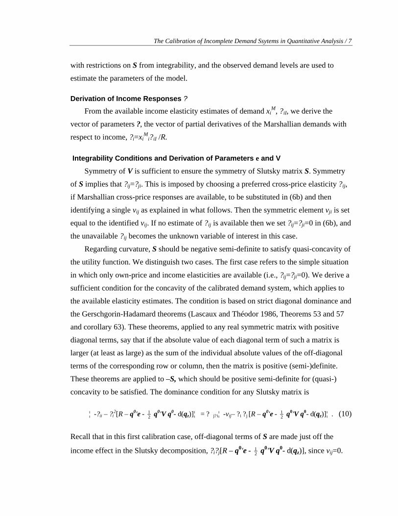
concavity to be satisfied. The dominance condition for any Slutsky matrix is

¦ -?ii – ?i2[R – q0'e - 1

2 q0'V q0- d(qz)]¦ = ? j? i¦ -vij– ?i ?j [R – q0'e - 12 q0'V q0- d(qz)]¦ . (10)

Recall that in this first calibration case, off-diagonal terms of S are made just off the

income effect in the Slutsky decomposition, ?i?j[R – q0'e - 12 q0'V q0- d(qz)], since vij=0.


In order to transform inequality (10) in elasticity terms, we momentarily normalize

prices q to one by appropriate choice of units and without any loss of generality.

Diagonal dominance condition (10) is preserved by adding on both sides the income

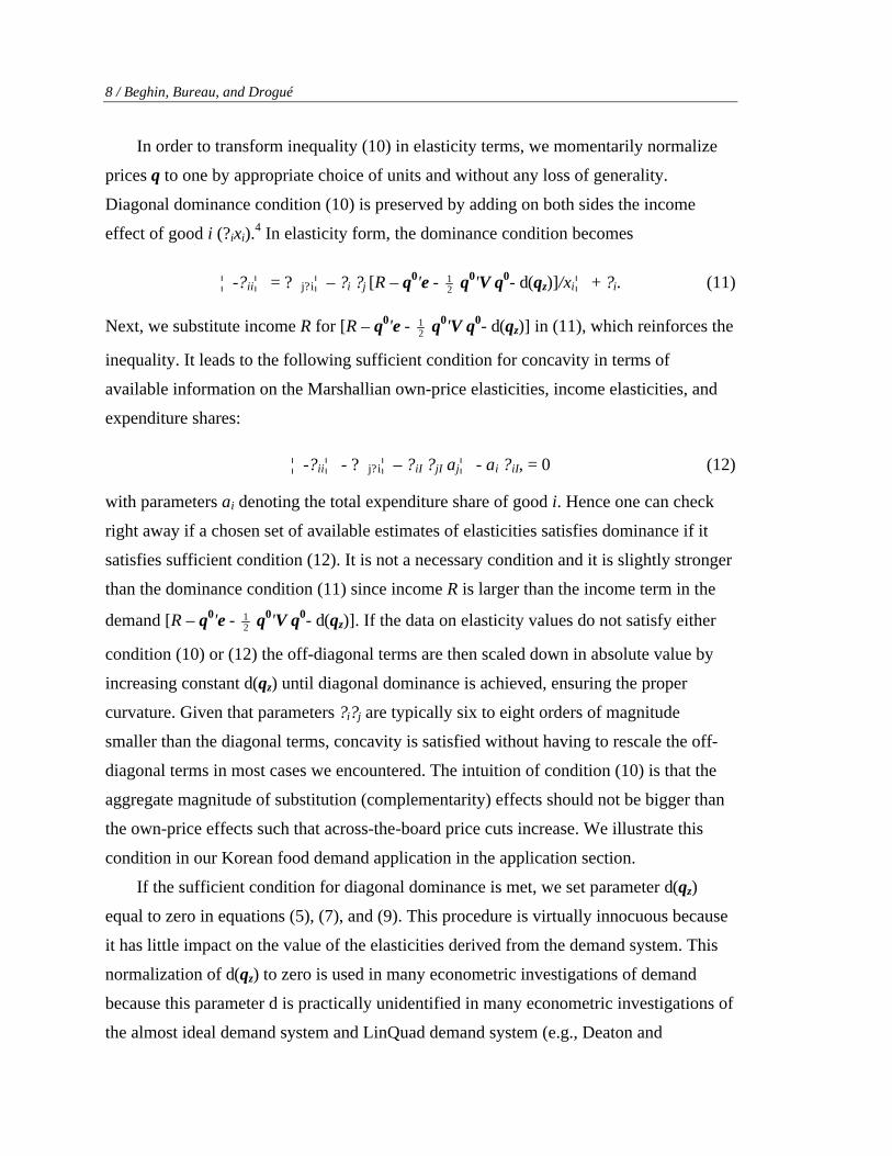
effect of good i (?ixi).4 In elasticity form, the dominance condition becomes

¦ -?ii¦ = ? j?i¦ – ?i ?j [R – q0'e - 12 q0'V q0- d(qz)]/xi¦ + ?i. (11)

Next, we substitute income R for [R – q0'e - 12 q0'V q0- d(qz)] in (11), which reinforces the

inequality. It leads to the following sufficient condition for concavity in terms of

available information on the Marshallian own-price elasticities, income elasticities, and

expenditure shares:

¦ -?ii¦ - ? j?i¦ – ?iI ?jI aj¦ - ai ?iI, = 0 (12)

with parameters ai denoting the total expenditure share of good i. Hence one can check

right away if a chosen set of available estimates of elasticities satisfies dominance if it

satisfies sufficient condition (12). It is not a necessary condition and it is slightly stronger

than the dominance condition (11) since income R is larger than the income term in the

demand [R – q0'e - 12 q0'V q0- d(qz)]. If the data on elasticity values do not satisfy either

condition (10) or (12) the off-diagonal terms are then scaled down in absolute value by

increasing constant d(qz) until diagonal dominance is achieved, ensuring the proper

curvature. Given that parameters ?i?j are typically six to eight orders of magnitude

smaller than the diagonal terms, concavity is satisfied without having to rescale the off-

diagonal terms in most cases we encountered. The intuition of condition (10) is that the

aggregate magnitude of substitution (complementarity) effects should not be bigger than

the own-price effects such that across-the-board price cuts increase. We illustrate this

condition in our Korean food demand application in the application section.

If the sufficient condition for diagonal dominance is met, we set parameter d(qz)

equal to zero in equations (5), (7), and (9). This procedure is virtually innocuous because

it has little impact on the value of the elasticities derived from the demand system. This

normalization of d(qz) to zero is used in many econometric investigations of demand

because this parameter d is practically unidentified in many econometric investigations of

the almost ideal demand system and LinQuad demand system (e.g., Deaton and


Muellbauer 1980; Fang and Beghin 2002). Large variations in its value have little bearing

on the values of ε and V and the exact welfare measure.5 Other values for d are obviously

defensible.

In the second case related to concavity, estimates for some cross-price effects are

available. Typically, the degree of knowledge and confidence of the analyst on these

cross-price effects is limited. Our approach is to leave income and own-price responses

unchanged and to scale down cross-price effects if conditions for concavity are not met.

We scale the cross-price effects in absolute value until the concavity sufficient condition

is satisfied either through diagonal dominance (10) or through Cholesky factorization

(Lau 1978).6 In this second case, the scaling affects mostly the cross-slope coefficients ?ij

and then the intercept terms εi, which in turn affect the values of the own-price responses

in the Slutsky matrix via feedback on the income term [R – q0'e - 12 q0'V q0- d(qz)] in

Marshallian demands. One could check sequentially if own-price and income elasticities

are consistent as a separate set of estimates using the first-case approach, then move to

the second case and use the additional estimates of cross-price effects to constrain the

whole set of available elasticity estimates.

With ? being identified in the previous step, its values are then combined with

available information on the level of demand (equation (5)) and elasticities (6), (own-

price elasticities, and if available, cross-price elasticity estimates) to recover structural

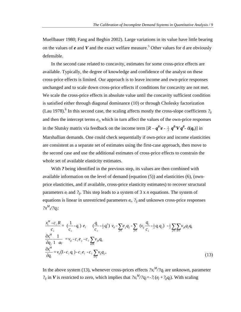
parameters ei and ?ij. This step leads to a system of 3 x n equations. The system of

equations is linear in unrestricted parameters ei, ?ij and unknown cross-price responses

?xMi/?qj:

=∂∂

=+∂

∂

+

=

∑

∑

∑∑∑∑

≠

≠ ≠≠≠

,--)-1(

--1

1

-)-(--)-()-1

(-

21

212

21

jijijiiiiiii

i

Mi

allkkjkijiij

ijj

Mi

kjij ik

jkij

jii

jij

ijjjiii

i

iii

ii

iMi

qvqvqx

qvvaq

x

qqvqqq

vqvqq

qRx

χεχχ

χεχ

χε

χε

χχχ

(13)

In the above system (13), whenever cross-prices effects ?xiM/?qj are unknown, parameter

?ij in V is restricted to zero, which implies that ?xiM/?qj=-?i (ej +?jjqj). With scaling


parameters aij set to zero, the system of equations in e and V is exactly identified. To

impose curvature restrictions the scaling parameters aij are set non-negative and chosen

by minimizing the sum of corrections ? i? j aij, which satisfies system (13) and condition

(10). The non-negative constraint preserves the sign of the estimates of the

substitution/complementarity effects.

With the calibrated values of the elements of V and e, the EV is calibrated, and

welfare analysis of price changes is possible. We use the GAMS DNLP solver, which

handles absolute values.

Application to Korea

We now turn to our illustration for the case of Korea. We look at an incomplete food

demand system for a representative Korean agent consuming the following commodities:

rice, barley, wheat, corn, soybean, dairy, beef, pork, and poultry. Korea provides a good

illustration because consumer prices are distorted and induce large consumer welfare

losses. We have various income and price elasticity estimates available, including six

cross-price effects between the three cereals and the three meats. The sources are various

and are detailed in Beghin, Bureau, and Park (2002). Table 1 summarizes the available

information on elasticity values, consumption levels, and relative prices in 1995 won.

We start with the first case in which we assume that only own-price and income

TABLE 1. Available data for calibration of a partial demand system in Korea (2000 data)

Goods

Quantities

Domestic Prices (q0)

World Prices (q1)

Own-Price Elasticity ?ii

Income Elasticities

?iI Rice 5126.00 1657.55 259.88 -0.20 0.12 Barley 467.00 417.08 133.19 -0.60 0.24 Wheat 3173.32 182.42 182.00 -0.40 0.18 Corn 9425.38 153.51 152.68 -0.45 0.43 Soybean 1815.00 358.21 213.58 -0.32 0.32 Milk 2753.00 497.51 131.56 -0.57 0.57 Beef 585.00 6348.26 1914.96 -0.80 0.54 Pork 1012.00 1961.03 1215.87 -0.89 0.73 Poultry 427.00 1692.37 1199.11 -0.70 0.37

Notes: Income = 475.830 billion won (1995 prices); cross-price elasticities: ?rice wheat = 0.08; ?barley wheat = 0.21; ?barley corn = 0.15; ?beef pork = 0.22; ?beef poultry = 0.04; ?pork poultry = 0.04.


elasticities are available to the researcher. These elasticity values and implied expenditure

shares satisfy the dominance condition (12) (for rice, 0.19647; barley, 0.59665; wheat,

0.39736; corn, 0.44338; soybeans, 0.31533; milk, 0.56150; beef, 0.79068; pork, 0.87920;

and poultry, 0.69459). Hence, no correction is required, and parameter d(qz) is set equal

to zero. Table 2 shows the implied Hicksian price-elasticity values implied by the

calibration for the diagonal case. The Hicksian cross-price response elasticities generated

by the calibration procedure are small but fully consistent with an integrable demand

system and lead to an exact welfare measure. They are positive as expected because all

goods are normal in this illustration. Indeed, when any vij is restricted to be equal to zero,

then the sign of the product of the income responses for good i and j, ?i ?j , determines the

sign of the substitution effect between goods i and j. The implied Marshallian elasticities

are shown in Table 3. Marshallian cross-price effects are negative because the correction

for the income effect is larger than the small positive substitution effect.

In the second calibration case, we make use of all available cross-price elasticities. The

diagonal dominance condition requires that we scale down by 26.9 percent the wheat-rice

cross-price effect. Table 4 gives the Slutsky price responses, and Table 5 gives the implied

Marshallian elasticities. We also show the corresponding results when the curvature

restriction is imposed via Cholesky factorization (Tables 6 and 7), which implies scaling

the wheat-rice price effect by 12.9 percent. Results are qualitatively similar between the

two approaches to impose curvature. Diagonal dominance induces a slightly larger

adjustment of the estimate of the cross-price response between wheat and rice than does the

Cholesky factorization. This is expected since the former method is a sufficient but not

necessary condition, whereas the latter is necessary and sufficient to establish positive

semi-definiteness of a symmetric real matrix.

Next, we simulate a large policy shock equivalent to full trade liberalization and

measure the EV corresponding to the price changes from domestic prices to border

prices. We do so for the two calibration cases (no off-diagonal information, the polar case

with information on six cross-price responses and curvature restrictions under both

diagonal dominance and Cholesky factorization). Table 8 shows the three EV estimates.

As shown in the table, the EV measures do change somewhat but the order of magnitude

of the impact of the price shock does not. The three EV measures are between 13.7 and

14 billion won, and income is 476 billion won. Hence, we conclude the EV measure is

robust to the inclusion or absence of available estimates of cross-price effects.

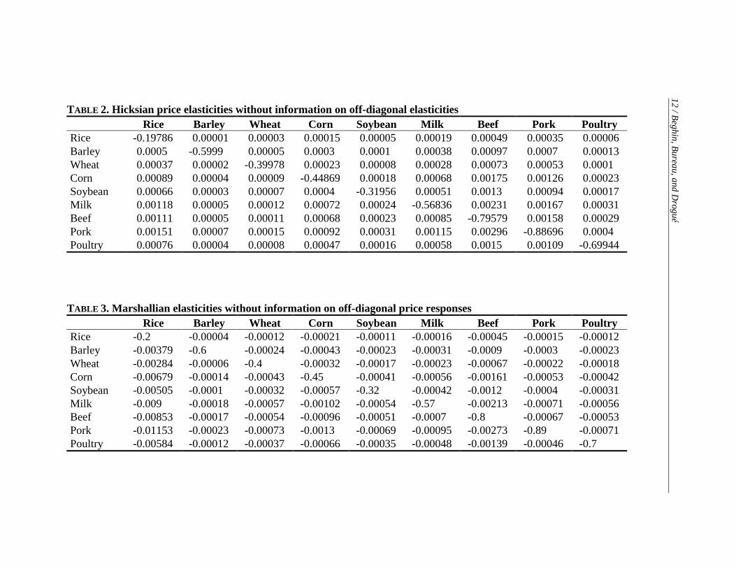
TABLE 2. Hicksian price elasticities without information on off-diagonal elasticities

Rice Barley Wheat Corn Soybean Milk Beef Pork Poultry Rice -0.19786 0.00001 0.00003 0.00015 0.00005 0.00019 0.00049 0.00035 0.00006 Barley 0.0005 -0.5999 0.00005 0.0003 0.0001 0.00038 0.00097 0.0007 0.00013 Wheat 0.00037 0.00002 -0.39978 0.00023 0.00008 0.00028 0.00073 0.00053 0.0001 Corn 0.00089 0.00004 0.00009 -0.44869 0.00018 0.00068 0.00175 0.00126 0.00023 Soybean 0.00066 0.00003 0.00007 0.0004 -0.31956 0.00051 0.0013 0.00094 0.00017 Milk 0.00118 0.00005 0.00012 0.00072 0.00024 -0.56836 0.00231 0.00167 0.00031 Beef 0.00111 0.00005 0.00011 0.00068 0.00023 0.00085 -0.79579 0.00158 0.00029 Pork 0.00151 0.00007 0.00015 0.00092 0.00031 0.00115 0.00296 -0.88696 0.0004 Poultry 0.00076 0.00004 0.00008 0.00047 0.00016 0.00058 0.0015 0.00109 -0.69944

TABLE 3. Marshallian elasticities without information on off-diagonal price responses

Rice Barley Wheat Corn Soybean Milk Beef Pork Poultry Rice -0.2 -0.00004 -0.00012 -0.00021 -0.00011 -0.00016 -0.00045 -0.00015 -0.00012 Barley -0.00379 -0.6 -0.00024 -0.00043 -0.00023 -0.00031 -0.0009 -0.0003 -0.00023 Wheat -0.00284 -0.00006 -0.4 -0.00032 -0.00017 -0.00023 -0.00067 -0.00022 -0.00018 Corn -0.00679 -0.00014 -0.00043 -0.45 -0.00041 -0.00056 -0.00161 -0.00053 -0.00042 Soybean -0.00505 -0.0001 -0.00032 -0.00057 -0.32 -0.00042 -0.0012 -0.0004 -0.00031 Milk -0.009 -0.00018 -0.00057 -0.00102 -0.00054 -0.57 -0.00213 -0.00071 -0.00056 Beef -0.00853 -0.00017 -0.00054 -0.00096 -0.00051 -0.0007 -0.8 -0.00067 -0.00053 Pork -0.01153 -0.00023 -0.00073 -0.0013 -0.00069 -0.00095 -0.00273 -0.89 -0.00071 Poultry -0.00584 -0.00012 -0.00037 -0.00066 -0.00035 -0.00048 -0.00139 -0.00046 -0.7

12 / Beghin, Bureau, and D

rogué

TABLE 4. Hicksian price elasticity estimates, diagonal dominance condition


Note: The wheat-rice cross-price effect is scaled down by 26.9%. TABLE 5. Marshallian elasticity estimates, diagonal dominance condition

Rice Barley Wheat Corn Soybean Milk Beef Pork Poultry Rice -0.20000 -0.00004 0.06306 -0.00021 -0.00011 -0.00016 -0.00045 -0.00015 -0.00012 Barley -0.00379 -0.60000 0.21000 0.15000 -0.00023 -0.00031 -0.00090 -0.00030 -0.00023 Wheat 0.92456 0.07068 -0.40000 -0.00032 -0.00017 -0.00023 -0.00067 -0.00022 -0.00018 Corn -0.00679 0.02011 -0.00043 -0.45000 -0.00041 -0.00056 -0.00161 -0.00053 -0.00042 Soybean -0.00505 -0.00010 -0.00032 -0.00057 -0.32000 -0.00042 -0.00120 -0.00040 -0.00031 Milk -0.00900 -0.00018 -0.00057 -0.00102 -0.00054 -0.57000 -0.00213 -0.00071 -0.00056 Beef -0.00853 -0.00017 -0.00054 -0.00096 -0.00051 -0.00070 -0.80000 0.22000 0.04000 Pork -0.01153 -0.00023 -0.00073 -0.00130 -0.00069 -0.00095 0.41020 -0.89000 0.04000 Poultry -0.00584 -0.00012 -0.00037 -0.00066 -0.00035 -0.00048 0.20689 0.11135 -0.70000

Note: The wheat-rice cross-price effect is scaled down by 26.9%.

The Calibration of Incom

plete Dem

and Ssytems in Q

uantitative Analysis / 13

TABLE 6. Hicksian elasticity estimates, Cholesky factorization


Note: The wheat-rice cross-price effect is scaled down by 12.9%. TABLE 7. Marshallian elasticity estimates, Cholesky factorization

Rice Barley Wheat Corn Soybean Milk Beef Pork Poultry Rice -0.20000 -0.00053 0.07016 -0.00165 -0.00135 -0.00175 -0.00199 -0.00235 -0.00214 Barley 0.00015 -0.60000 0.20990 0.15041 -0.00015 0.00004 0.00055 -0.00003 -0.00026 Wheat 1.04218 0.07074 -0.40000 0.00017 0.00003 0.00023 0.00067 0.00024 0.00003 Corn -0.00062 0.01989 -0.00090 -0.45000 -0.00084 -0.00073 -0.00003 -0.00110 -0.00138 Soybean 0.00004 -0.00014 -0.00050 -0.00015 -0.32000 -0.00009 0.00056 -0.00023 -0.00051 Milk -0.00056 -0.00041 -0.00111 -0.00081 -0.00096 -0.57000 0.00025 -0.00116 -0.00157 Beef -0.00250 -0.00089 -0.00170 -0.00240 -0.00218 -0.00247 -0.80000 0.21724 0.03703 Pork -0.00023 -0.00040 -0.00125 -0.00062 -0.00090 -0.00050 0.41383 -0.89000 0.03921 Poultry 0.00028 -0.00011 -0.00051 0.00001 -0.00020 0.00010 0.20918 0.11182 -0.70000 Note: The wheat-rice cross-price effect is scaled down by 12.9%.

14 / Beghin, Bureau, and D

rogué


TABLE 8. Equivalent variation for the removal of price distortions Without information on off-diagonal 13.95086 With information and diagonal dominance 13.70318 With information and Cholesky 13.70355 Note: Units are in billion won at 1995 prices.

Conclusions

This paper is a methodological contribution to quantitative economic analysis and

more particularly to the calibration of partial systems involving a subset of disaggregated

goods. We propose and illustrate an easily implemented and flexible calibration

technique for partial demand systems, combining recent developments in incomplete

demand systems and a set of restrictions conditioned on the available elasticity estimates

and integrability.

The technique accommodates various degrees of knowledge on cross-price

elasticities and allows the recovery of an exact welfare measure. It generates values for

missing cross-price elasticities, which are consistent with the available estimates. The

approach is illustrated with a partial demand system for food consumption in Korea for

different states of knowledge on cross-price effects. The consumer welfare impact of

food and agricultural trade liberalization is measured and is shown not to be sensitive to

the inclusion or deletion of available estimates of cross-price effects.

Curvature restrictions are imposed using alternative approaches (diagonal dominance

and Cholesky factorization). Diagonal dominance provides a sufficient condition for

concavity of utility, which can be expressed in terms of available estimates of

Marshallian own-price and income elasticities. This condition provides a direct and

convenient check of the estimates available to the policy analyst. The drawback of the

diagonal dominance approach is that it might impose adjustments in estimates that are

larger than what is necessary to satisfy curvature. Cholesky factorization does not allow

for a “quick” check of available estimates of own-price and income elasticities. However,

it does provide minimum adjustments in estimates that are necessary for curvature

restrictions to be satisfied. In our calibration illustration, the two methods for imposing

proper curvature yield very close estimates of preferences parameters and EV measures

for the policy changes.

Endnotes

1. For n goods, the number of price elasticities to estimate is equal to {n(n+1)/2}, assuming symmetry is imposed in a calibration using deflated prices; n income elasticities have to be found as well.

2. We define concavity (quasi-concavity) of utility with the condition that the Slutsky matrix of compensated price responses of the demand system is negative definite (negative semi-definite).

3. If only expenditures are known, quantity units for each good are redefined so that the associated price is equal to 1 per unit.

4. We rule out Giffen goods (income term smaller in absolute value to the Hicksian price term in absolute value in the Slutsky decomposition).

5. The sensitivity of EV with respect to d(qz) (dEV/dd(qz)) is 0.007 (an additional 1 million won in the income argument via d(qz) induces 7,000 won of variation in EV, which is of the order of 14 billion won for the price change considered in the illustration).

6. The Cholesky factorization decomposes minus the Slutsky matrix -S into -S=LlDLh, where D is a diagonal matrix constrained to have nonnegative elements Dii for quasi-concavity of the utility function, Ll is a unit lower triangular matrix, and Lh is the transpose of Ll (Lau). We use a similar scaling approach for the Cholesky factoriza-tion as for the diagonal-dominance approach. Scaling factors are applied to the slope estimates of the Marshallian cross-price effects to satisfy curvature restrictions (Dii) positive.

References

Baltas, G. 2002. “An Applied Analysis of Brand Demand Structure.” Applied Economics 34(9): 1171-75.

Beghin, J.C., J-C. Bureau, and S.J. Park. 2002. “Food Security and Protection in Agriculture in South Korea.” Working paper (revised September), Department of Economics, Iowa State University, Ames, Iowa. http://www.econ.iastate.edu/research/viewabstract.asp?pid=10044 (accessed December 2003).

Deaton, A., and J. Muellbauer. 1980. “An Almost Ideal Demand System.” American Economic Review 70(3, June): 312-26.

Fang, C., and J.C. Beghin. 2002. “Urban Demand for Edible Oils and Fats in China. Evidence from Household Survey Data.” Journal of Comparative Economics 30: 1-22.

Keller, W.J. 1984. “Some Simple but Flexible Differential Consumer Demand Systems.” Economics Letters 16: 77-82.

Lascaux, P., and R. Théodor. 1986. Analyse Numérique Matricielle Appliquée à l’Art de L’Ingénieur, vol. 1. Paris: Masson P.

LaFrance, J.T. 1985. “Linear Demand Functions in Theory and Practice.” Journal of Economic Theory 37: 147-66.

———. 1998. “The LINQUAD Incomplete Demand Model.” Working Paper, Department of Agricultural and Resource Economics, University of California, Berkeley.

LaFrance, J.T., and W.M. Hanemann. 1989. “The Dual Structure of Incomplete Demand Systems.” American Journal of Agricultural Economics 71: 262-74.

LaFrance, J.T., T.K.M. Beatty, R.D. Pope, and G.K. Agnew. 2002. “The U.S. Distribution of Income and Gorman Engel Curves for Food.” Journal of Econometrics 107: 235-57.

Lau, L.J. 1978. “Testing and Imposing Monotonicity, Convexity, and Quasi-Convexity Constraints.” Appendix A4 in Production Economics: A Dual Approach to Theory and Applications. Edited by M. Fuss and D. McFadden. Amsterdam: North Holland.

Moschini, G. 2001. “A Flexible Multistage Demand System Based on Indirect Separability.” Southern Economic Journal 68(1): 22-41.

———. 1999. “Specification of the Demand Structure of National Models and Welfare Calculations.” Memorandum prepared for the U.S. Department of Agriculture-World Trade Organization Project, Ames, Iowa. February.

Organisation for Economic Cooperation and Development (OECD). 2000. “A Matrix Approach to Evaluation Policy: Preliminary Findings from the PEM Pilot Studies of Crop Policy in the EU, the US, Canada and Mexico.” Document COM/AGR/CA/TD/TC/(99)117. Paris. March.


Roningen, V., J. Sullivan, and P. Dixit. 1991. “Documentation of the Static World Policy Simulation (SWOPSIM) Modeling Framework.” U.S. Department of Agriculture, ATAD, Economic Research Service. Washington, D.C. September.

Selvanathan, E.A. 1985. “An Even Simpler Differential Demand System.” Economics Letters 19: 343-47.

The Calibration of Incomplete Demand Systems in Quantitative...

Documents

Transcript of The Calibration of Incomplete Demand Systems in Quantitative...