
The Bureau’s Operational AWRA Landscape (AWRA-L) Model
55
The Bureau’s Operational AWRA Landscape (AWRA-L) Model Technical Description of AWRA-L version 5
Transcript of The Bureau’s Operational AWRA Landscape (AWRA-L) Model

The Bureau’s Operational AWRA Landscape (AWRA-L) Model Technical Description of AWRA-L version 5

The Bureau’s Operational AWRA-L Model: Technical description of AWRA-L version 5
Published by the Bureau of Meteorology
Citation: Frost, A. J., Ramchurn, A., and Smith, A. (2016) The Bureau’s Operational AWRA Landscape (AWRA-L) Model. Bureau of Meteorology Technical Report.
Version number/type Date of issue
4
23/11/2016
© Commonwealth of Australia 2016
This work is copyright. Apart from any use as permitted under the Copyright Act 1968, no part may be reproduced without prior written permission from the Bureau of Meteorology. Requests and inquiries concerning reproduction and rights should be addressed to the Production Manager, Communication Section, Bureau of Meteorology, GPO Box 1289, Melbourne 3001. Information regarding requests for reproduction of material from the Bureau website can be found at www.bom.gov.au/other/copyright.shtml

The Bureau’s Operational AWRA-L Model
i
Contact details
Dr. Andrew Frost
Manager (acting) - Water Resources Modelling Unit
Bureau of Meteorology
PO Box 413, Darlinghurst NSW 1300
Tel: +61 2 9296 1517
Email: [email protected]
Dr. Amgad Elmahdi
Section Head, Water Resources Assessment
Bureau of Meteorology GPO Box 1289 Melbourne VIC 3001
Tel: +61 3 8638 8274 Email: [email protected]

The Bureau’s Operational AWRA-L Model: Technical description of AWRA-L version 5
ii
Summary
This technical report provides a detailed description of the Bureau of Meteorology's Operational Australian Water Resources Assessment Landscape model: AWRA-L version 5. The report includes a description of:
the overall conceptual structure
the model components (water balance, vapour fluxes and the energy balance, and vegetation phenology), and
how the model was parameterised nationally
Process equations are provided along with brief background on their choice and individual parameterisation.
The parameterisation described is as used to produce outputs on the operational Australian Landscape Water Balance website www.bom.gov.au/water/landscape.
Coding references are as implemented in the Bureau of Meteorology's AWRA Community Modelling system.
A reference guide for parameters used in the model code and within this document is provided in Appendix A.

The Bureau’s Operational AWRA-L Model
iii
Table of Contents
1 Introduction ................................................................................................................................................... 1
1.1 The AWRA modelling system ........................................................................................................... 1
1.2 Conceptual structure .......................................................................................................................... 3
1.3 Spatial data and Hydrologic Response Units (HRUs) ................................................................... 6
1.3.1 Input climate data ........................................................................................................................... 6
1.3.2 Static spatial datasets .................................................................................................................... 7
1.3.3 HRU proportions (ftree) .................................................................................................................... 8
1.4 Structure of this report ........................................................................................................................ 9
2 Water balance ............................................................................................................................................ 10
2.1 Water balance equations ................................................................................................................. 11
2.1.1 Surface runoff (𝑄𝑅 = 𝑄ℎ + 𝑄𝑠) ................................................................................................... 12
2.1.2 Soil storage (𝑆0, 𝑆𝑠, 𝑆𝑑), drainage (𝐷0, 𝐷𝑠, 𝐷𝑑) and interflow (𝑄𝐼𝐹 = 𝑄𝐼0 + 𝑄𝐼𝑠) ................ 13
2.1.3 Groundwater storage (𝑆𝑔) and fluxes (𝑄𝑔, 𝐸𝑔, 𝑌 ) ................................................................... 17
2.1.4 Total Streamflow and surface water storage ............................................................................ 19
3 Vapour fluxes and the energy balance ................................................................................................... 21
3.1 Potential evaporation (𝐸0) ............................................................................................................... 21
3.2 The energy balance .......................................................................................................................... 22
3.2.1 Upward and Downward shortwave radiation ............................................................................ 22
3.2.2 Upward longwave radiation ......................................................................................................... 23
3.2.3 Downward longwave radiation .................................................................................................... 23
3.3 Actual evapotranspiration (𝐸𝑡𝑜𝑡) .................................................................................................... 24
3.3.1 Interception evaporation (𝐸𝑖) ...................................................................................................... 24
3.3.2 Soil evaporation (𝐸𝑠) ................................................................................................................... 25
3.3.3 Evaporation from groundwater (𝐸𝑔)........................................................................................... 25
3.3.4 Root water uptake from (𝐸𝑡 = 𝑈𝑠 + 𝑈𝑑) .................................................................................... 25
3.3.5 Transpiration from groundwater (𝑌) ........................................................................................... 28
4 Vegetation Phenology ............................................................................................................................... 29
5 Parameterisation ........................................................................................................................................ 32
References .......................................................................................................................................................... 36

The Bureau’s Operational AWRA-L Model: Technical description of AWRA-L version 5
iv
Appendices .......................................................................................................................................................... 41
Appendix A: Table of model variables ............................................................................................................. 42
Appendix B: Downward longwave radiation derivation ................................................................................. 45

The Bureau’s Operational AWRA-L Model
v
List of Tables
Table 1. List of AWRA-L parameter values. Values that apply to either the deep or shallow
rooted HRU (or both) are provided. Values that are optimised are shown in bold. .................... 34
Table 2. List of variable names used in this document and the corresponding variables used
in the model code. Units are those given in this document. ......................................................... 42
List of Figures
Figure 1. Conceptual AWRA-L grid cell with key water stores and fluxes shown ................... 4
Figure 2. AWRA-L conceptual structure. Purple: climate inputs; Blue rounded boxes: water stores; red boxes: water flux outputs; brown: energy balance; green rounded boxes vegetation
processes. Dotted line indicates HRU processes. ............................................................. 5
Figure 3. Wind speed climatology (𝑢2) ............................................................................ 6
Figure 4. Fraction deep rooted vegetation within each grid cell (ftree) ................................... 9
Figure 5. AWRA-L hydrological processes. Blue rounded boxes indicate water storages, white
if no storage, white boxes are water balance fluxes, and red boxes are the output fluxes. ....10
Figure 6. Continental distribution of reference precipitation (𝑃𝑟𝑒𝑓).....................................13
Figure 7. Saturated conductivity (𝐾𝑥𝑠𝑎𝑡) and maximum soil storage (𝑆𝑥𝑚𝑎𝑥) for the top (0),
shallow (s) and deep (d) soil layers. ...............................................................................15
Figure 8. Average slope (𝛽) within a grid from a 3 second DEM ........................................16
Figure 9. Groundwater drainage coefficient (𝐾𝑔 ) ............................................................17
Figure 10. Effective porosity (𝑛) ....................................................................................18
Figure 11. Hypsometric curve conversion of groundwater storage to fraction of cell saturated
and fraction of cell available for transpiration...................................................................19
Figure 12. Streamflow routing coefficient (𝐾𝑟 ) ................................................................20
Figure 13. Vegetation height of deep rooted vegetation (ℎ𝑣𝑒𝑔) .........................................28
Figure 14. Maximum Leaf Area Index (𝐿𝐴𝐼𝑚𝑎𝑥) ..............................................................31
Figure 15. Location of unimpaired catchments used for model evaluation with climate zones
overlain. .....................................................................................................................35

The Bureau’s Operational AWRA-L Model: Technical description of AWRA-L version 5
vi
List of Acronyms
AVHRR: Advanced Very High Resolution radiometer
AMSR-E: Advanced Microwave Scanning Radiometer for the Earth Observing System
ASRIS: Australian Soil Resource Information System
AWAP: Australian Water Availability Project
AWRA-L: Australian Water Resources Assessment Landscape Model
AWRA-R: Australian Water Resources Assessment River Model
AWRAMS: Australian Water Resource Assessment modelling system
BoM: Bureau of Meteorology
CMRSET: CSIRO MODIS reflectance-based Scaling ET
CSIRO: Commonwealth Scientific and Industrial Research Organisation
ET: Evapotranspiration
fPAR: fraction of Photosynthetically Active Radiation absorbed by vegetation
HRU: Hydrological Response Unit
LAI: Leaf Area Index
NWA: National Water Account
MODIS: Moderate Resolution Imaging Spectroradiometer
RWI: Regional Water Information
WIA: Water in Australia
WIRADA: Water Information Research and Development Alliance

The Bureau’s Operational AWRA-L Model
1
1.1 The AWRA modelling system
The Australian Water Resources Assessment Modelling System (AWRAMS) underpins the Bureau water information services that are mandated through the Water Act (2007). The science of AWRAMS (Vaze et al., 2013; see Elmahdi et al., 2015; Hafeez et al., 2015); has been developed since July 2008 through the Water Information Research and Development Alliance (WIRADA) between CSIRO and the Australian Bureau of Meteorology (hereafter the Bureau). The AWRAMS has been operational at the Bureau since 2011-12 for regular use in the National Water Account (NWA) and Water Resources Assessment reports. The AWRAMS has evolved from AWRA v 0.5 (Van Dijk, 2010c) to AWRA v 5.0 (Viney et al., 2015) with AWRA v 5.0 transferred from CSIRO, recoded, operationalised and is currently being used for reporting purposes by the Bureau. While a prototype AWRAMS was developed through WIRADA, the AWRAMS has been significantly refactored and enhanced through the Bureau AWRAMS Implementation (AWRAMSI) project over the three years (2012-2015) for superior performance and less simulation and calibration time. AWRAMS was further enhanced by the addition of the best available national benchmarking datasets and tools for evaluation. The operational AWRAMS has been used towards supplying retrospective water balance estimates published by the Bureau within:
Water in Australia (www.bom.gov.au/water/waterinaustralia): an annual national picture of water availability and use in a particular financial year
Water resources assessments produced prior to Water In Australia (www.bom.gov.au/water/awra)
Regional water information water resource assessments (www.bom.gov.au/water/rwi)
National Water Account (NWA: www.bom.gov.au/water/nwa): that provides an annual set of water accounting reports for ten nationally significant water resource management regions. Adelaide, Burdekin, Canberra, Daly, Melbourne, Murray–Darling Basin, Ord, Perth, South East Queensland and Sydney.
The Bureau’s AWRAMSI Project transferred, recoded, and operationalised the WIRADA prototype to make an operational AWRA modelling system that is more efficient, functional, and easily maintainable in a Linux platform maintained by the Bureau’s staff. It is a Python based modelling system, with the core model algorithms implemented in high performing native languages (Fortran, C) and generic functionality provided by robust, open source libraries. The operational AWRAMS simulates Australian landscape and river water stores and fluxes for the past 100 years to now (Hafeez et al., 2015). These estimates are updated on a daily basis and provide the current and historical context of water availability in Australia. There are two main components to the AWRA modelling system:
1 Introduction
The Bureau’s Operational AWRA-L Model: Technical description of AWRA-L version 5
2
AWRA-L: a one dimensional, 0.05 degree grid based landscape water balance model over the continent that has semi-distributed representation of the soil, groundwater and surface water stores. The AWRA-L model, operational since November 2015, publishes daily updated outputs to the public, with daily gridded soil moisture, runoff, evapotranspiration, and deep drainage outputs (see Figure 1) available from yesterday back to 1911 online through www.bom.gov.au/water/landscape.
AWRA-R: a node link network conceptual river model designed for both regulated and unregulated river system. Currently, implemented over a few regions (MDB, Melbourne and SEQ) for national water account purposes.
Since the operational AWRA-L modelled outputs have been made publicly available in November 2015, the modelled fluxes have been used internally and externally for various climatological, flood, water and agriculture applications across Australia. The Bureau’s AWRA team has been regularly interacting with a wide range of stakeholders about their needs and how these can be met by a daily operational water balance model. These interactions have spanned Commonwealth agencies and State government water and agriculture agencies, catchment management authorities, water utilities, consultants, water industry professionals, research organisations, universities and farmers.
This technical report describes the AWRA-L version 5.0 model structure and is intended to be used as a quick reference for the model equations and processes used in the Bureau's AWRA Community Modelling system. This document relies heavily on the following two prior descriptions of AWRA-L based on CSIROs research implementations of AWRA-L:
Van Dijk, A. I. J. M. (2010) The Australian Water Resources Assessment System. Technical Report 3. Landscape Model (version 0.5) Technical Description.
Viney, N., Vaze, J., Crosbie, R., Wang, B., Dawes, W. and Frost, A. (2015) AWRA-L v5.0: technical description of model algorithms and inputs. CSIRO, Australia.
Limited explanation is provided here for the derivation and choice of parameterisations. Van Dijk (2010c) provides the original design principles and the rational for choice of the original national parametrisation in v0.5. Viney et al. (2015) describes the improvements have been made in parameterisation and the conceptual structure of AWRA-L v5.0 towards better estimation of the outputs required from AWRA-L.

The Bureau’s Operational AWRA-L Model
3
1.2 Conceptual structure
AWRA-L (Van Dijk, 2010c; Viney et al., 2014; Viney et al., 2015) is a one dimensional, 0.05° grid based water balance model over the continent that has semi-distributed representation of the soil, groundwater and surface water stores. Within each grid cell there are three soil layers (top: 0-10cm, shallow: 10cm-100cm, deep: 100cm-600cm) and two hydrological response units (HRU: shallow rooted versus deep rooted). Shallow rooted vegetation is assumed to have roots to the extent of the shallow soil layer (to 1m), while deep rooted vegetation is assumed to have roots down to 6 m (ie. the extent of the deep soil layer).
Key fluxes and stores output by AWRA-L as output of the operational Australian Landscape Water Balance website www.bom.gov.au/water/landscape include runoff, actual evapotranspiration, soil moisture for the three soil layers and deep drainage to the groundwater store - Figure 1. It is noted differing naming is used for the soil layers on the website and Figure 1 (Upper, Lower and Deep soil) rather than what is used in this document (Top, Shallow and Deep soil). The naming used here is consistent with the code and previous documentation.

The Bureau’s Operational AWRA-L Model: Technical description of AWRA-L version 5
4
Figure 1. Conceptual AWRA-L grid cell with key water stores and fluxes shown
AWRA-L models hydrological processes for:
Partitioning of rainfall between interception losses and net rainfall
Saturation excess overland flow (depending on groundwater store saturation level)
Infiltration and Hortonian (infiltration excess) overland flow
Saturation, interflow, drainage and evaporation from soil layers
Baseflow, evaporation and transpiration from the groundwater store
with the soil layers modelled separately for 2 (shallow and deep rooted) hydrological response units. In addition, the following vegetation processes are described:
transpiration, as a function of maximum root water uptake and optimum transpiration rate;

The Bureau’s Operational AWRA-L Model
5
vegetation cover adjustment, as a function of the balance between the theoretical optimum and the actual transpiration, and at a rate corresponding to vegetation cover type.
The top, shallow and deep soil layer depths within AWRA-L are chosen to be 0.1m, 1m and 6m respectively. Differing model parameters are chosen where appropriate for the shallow and deep rooted HRU’s. Hydrologically, these two HRU’s differ in their aerodynamic control of evaporation, in their interception capacities and in their degree of access to different soil layers. Groundwater and river water dynamics are simulated at grid cell level and hence parameters are the same across the grid cell and dynamic variables (e.g. fraction groundwater saturated area and open water within stream channels) equal between HRUs.
Figure 2 shows the conceptual structure of the AWRA-L model (hereafter termed AWRA-L).
Figure 2. AWRA-L conceptual structure. Purple: climate inputs; Blue rounded boxes:
water stores; red boxes: water flux outputs; brown: energy balance; green rounded
boxes vegetation processes. Dotted line indicates HRU processes.

The Bureau’s Operational AWRA-L Model: Technical description of AWRA-L version 5
6
1.3 Spatial data and Hydrologic Response Units (HRUs)
1.3.1 Input climate data
The spatial resolution of AWRA-L is driven by the resolution of input climate data, namely 0.05° (approximately 5 km).
AWRA-L uses daily gridded Australian Water Availability Project (AWAP) climate data set that consists of air temperature (daily minimum and maximum) and daily precipitation from 1st January 1911 to yesterday (Jones et al., 2009).
The rainfall and temperature data is interpolated from station records and provided on a 0.05° grid across Australia. Additionally, daily solar exposure (downward shortwave radiation) is produced from geostationary satellites (Grant et al., 2008) and aggregated to the same 0.05° AWAP grid. The solar radiation record is from 1990 to yesterday, with the Himawari-8 satellite used since 23rd March 2016. Prior to that date the GMS-4, GMS-5, GOES-9 and MTSAT-1R satellites were used. Daily climatological averages (taken for each month) are used for solar radiation prior to 1990.
Long term daily average wind speed derived from data supplied by McVicar et al. (2008) was used for the wind speed within the AWRA-L. McVicar et al. (2008) interpolated daily Bureau site data, and then this data was averaged temporally (Figure 3) to generate a daily average value that is applied at all timesteps.
Figure 3. Wind speed climatology (𝒖𝟐)

The Bureau’s Operational AWRA-L Model
7
The following notation is used for the climate forcing in this report:
𝑃𝑔 Daily gross precipitation to 9am local time [mm]
𝐾𝑑 Daily downwelling shortwave (solar) radiation [MJ m–2 d–1]
𝑢2 Wind speed at a height of 2 m [m/s]
𝑇𝑚𝑖𝑛 Daily minimum air temperature to 9am local time [°C]
𝑇𝑚𝑎𝑥 Daily maximum air temperature from 9am local time [°C]
It is noted that the daily minimum and maximum air temperature actually cover two
adjacent days (a period of 48 hours) and it is possible to have 𝑇𝑚𝑖𝑛 > 𝑇𝑚𝑎𝑥 . A weighted average of these two values is taken to get an average temperature value for calculation of Potential Evaporation, with the 𝑇𝑚𝑖𝑛 being set to 𝑇𝑚𝑎𝑥 in cases
where 𝑇𝑚𝑖𝑛 > 𝑇𝑚𝑎𝑥 – see section 3.1.
1.3.2 Static spatial datasets
Various static spatial datasets are used to parameterise AWRA-L spatially. These spatial grids (discussed subsequently within the document) are as follows:
ftree The HRU proportion of deep rooted vegetation in each cell (Figure 4). This also the proportion of the shallow HRUs within each grid cell (see section 1.3.3)
𝑃𝑟𝑒𝑓𝑚𝑎𝑝 Reference precipitation [mm/d] controlling infiltration-excess runoff
further derived from slope 𝛽 and 𝐾0𝑠𝑎𝑡𝑃𝐸𝐷𝑂 using an empirical relationship (see section 2.1.1). Figure 6 shows the final value used in AWRA-L v5 after scaling of the mapped value according to model parameter optimisation.
𝐾𝑥𝑠𝑎𝑡𝑃𝐸𝐷𝑂 Saturated hydraulic conductivity [mm/d] for the top (𝑥=0), shallow (𝑥=s) and deep (𝑥=d) layers defining the drainage rate when saturated (see section 2.1.2). These values were derived using pedotransfer functions based on clay content. Figure 7 shows the final value used in v5 after scaling of the mapped values according to model parameter optimisation.
𝑆𝑥𝐴𝑊𝐶 Available water storage fraction for top (𝑥=0) and shallow (𝑥=s) layers (see section 2.1.2). These values were derived from available mapping, with the deep (𝑥=d) layer value a scaled value of the shallow layer. Figure 7 shows the final value used in v5 after scaling of the mapped values according to model parameter optimisation.
𝛽 Slope of the land surface [percent] derived according to Digital Elevation Model (DEM) analysis (Figure 8). Slope affects infiltration excess runoff (through Reference precipitation 𝑃𝑟𝑒𝑓; see section 2.1.1)

The Bureau’s Operational AWRA-L Model: Technical description of AWRA-L version 5
8
and the proportion of drainage that occurs laterally as interflow (section 2.1.2).
𝐾𝑔𝑚𝑎𝑝 The groundwater drainage coefficient controls the baseflow rate – see
section 2.1.3. Figure 9 shows the final value used in v5 after scaling of the mapped values according to model parameter optimisation.
𝑛𝑚𝑎𝑝 Effective porosity affects lateral groundwater flow (baseflow; through
𝐾𝑔𝑚𝑎𝑝), along with the fraction saturated groundwater (which effects
the amount of saturated overland flow) and fraction of groundwater available transpiration (Figure 10)
Hypsometric curves The hypsometric curve is the cumulative distribution of elevation within an AWRA-L grid cell, based on a finer scale DEM. This is used for conversion from groundwater storage to head relative to the lowest point in the cell. The head level determines the fraction saturated groundwater (which effects the amount of saturated overland flow) and fraction of groundwater available transpiration – see section 2.1.3.
𝐸∗ Long term mean daily evapotranspiration is related by and empirical equation to the routing delay for streamflow (Figure 12)
ℎ𝑣𝑒𝑔 Vegetation height of deep rooted vegetation (i.e. to the top of the
canopy for tall vegetation and derived from lidar estimates) alters the aerodynamic conductance (Figure 13)
𝐿𝐴𝐼𝑚𝑎𝑥 Maximum leaf area index (Figure 14) defines the maximum achievable canopy cover in a particular cell.
The figures referenced above show the resulting parameters used in AWRA-L, often according to a transformation of scaling undertaken as a result of the calibration process.
1.3.3 HRU proportions (ftree)
Each spatial unit (grid cell) in AWRA-L is divided into a number of hydrological response units (HRUs) representing different landscape components. Hydrological processes (with the exception of groundwater storage) are modelled separately for each HRU before the resulting fluxes are combined to give cell outputs, by a weighted sum according to the proportion of each HRU. The current version of AWRA-L includes two HRUs which notionally represent (i) tall, deep-rooted vegetation (i.e., forest), and (ii) short, shallow-rooted vegetation (i.e., non-forest). Hydrologically, these two HRUs differ in their aerodynamic control of evaporation, in their interception capacities and in their degree of access to different soil layers.
The Bureau’s Operational AWRA-L Model
9
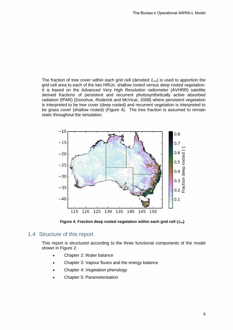
The fraction of tree cover within each grid cell (denoted ftree) is used to apportion the grid cell area to each of the two HRUs: shallow rooted versus deep rooted vegetation. It is based on the Advanced Very High Resolution radiometer (AVHRR) satellite derived fractions of persistent and recurrent photosynthetically active absorbed radiation (fPAR) (Donohue, Roderick and McVicar, 2008) where persistent vegetation is interpreted to be tree cover (deep rooted) and recurrent vegetation is interpreted to be grass cover (shallow rooted) (Figure 4). The tree fraction is assumed to remain static throughout the simulation.
Figure 4. Fraction deep rooted vegetation within each grid cell (ftree)
1.4 Structure of this report
This report is structured according to the three functional components of the model shown in Figure 2:
Chapter 2: Water balance
Chapter 3: Vapour fluxes and the energy balance
Chapter 4: Vegetation phenology
Chapter 5: Parameterisation

The Bureau’s Operational AWRA-L Model: Technical description of AWRA-L version 5
10
Figure 5 shows a conceptual diagram of the water balance processes modelled in AWRA-L. These processes are described in this section.
Figure 5. AWRA-L hydrological processes. Blue rounded boxes indicate water storages,
white if no storage, white boxes are water balance fluxes, and red boxes are the output
fluxes.
2 Water balance
The Bureau’s Operational AWRA-L Model
11
2.1 Water balance equations
All water storage and daily flux terms have millimetres [mm] for units. Throughout the document (t) is used to denote the value corresponding to day t. All calculations below are undertaken for the shallow and deep rooted HRUs separately, with the exception of the groundwater balance (considered as a single store) and total stream discharge (which are from a weighted sum of the flows over the two HRUs).
Gross rainfall (𝑃𝑔) [mm] from the interpolated gridded daily input data after subtracting
evaporation due to canopy interception (𝐸𝑖), assuming no canopy storage, gives the net rainfall (𝑃𝑛):
𝑃𝑛(𝑡) = {𝑃𝑔(𝑡) − 𝐸𝑖(𝑡), 𝑃𝑔 > 𝐸𝑖
0, 𝑃𝑔 ≤ 𝐸𝑖 (1)
Soil surface partitioning of net rainfall into surface runoff (𝑄𝑅) and infiltration (𝐼) gives:
𝐼(𝑡) = 𝑃𝑛(𝑡) − 𝑄𝑅(𝑡) (2)
Top soil water balance, comprising top soil water storage (𝑆0), infiltration, soil evaporation
(𝐸𝑠), interflow draining laterally from the top soil layer (𝑄𝐼0) and top soil drainage (𝐷0):
𝑆0(𝑡) = 𝑆0(𝑡 − 1) + 𝐼(𝑡) − 𝐷0(𝑡) − 𝑄𝐼0(𝑡) − 𝐸𝑠(𝑡) (3)
Shallow soil water balance, comprising shallow soil water storage (𝑆𝑠), shallow root water uptake (𝑈𝑠 ), top soil drainage (𝐷0) from the layer above, interflow draining
laterally from the shallow soil layer (𝑄𝐼𝑠) and shallow soil water drainage (𝐷𝑠):
𝑆𝑠(𝑡) = 𝑆𝑠(𝑡 − 1) + 𝐷0(𝑡) − 𝐷𝑠(𝑡) − 𝑄𝐼𝑠(𝑡) − 𝑈𝑠(𝑡) (4)
Deep soil water balance, comprising deep soil water storage (𝑆𝑑), 𝐷𝑠, deep root water uptake (𝑈𝑑), and deep drainage (𝐷𝑑):
𝑆𝑑(𝑡) = 𝑆𝑑(𝑡 − 1) + 𝐷𝑠(𝑡) − 𝐷𝑑(𝑡) − 𝑈𝑑(𝑡) (5)
Groundwater balance, comprising ground water storage (𝑆𝑔), 𝐷𝑑, root water uptake
from groundwater store (𝑌), groundwater evaporation (𝐸𝑔) and groundwater discharge
(𝑄𝑔):
𝑆𝑔(𝑡) = 𝑆𝑔(𝑡 − 1) + 𝑫𝒅(𝑡) − 𝑸𝒈(𝑡) − 𝑬𝒈(𝑡) − 𝒀(𝑡) (6)
with each flux component a weighted sum according to the fraction HRU – denoted in bold here.
River water balance, comprising surface water storage (𝑆𝑟 ), surface runoff (𝑄𝑅) , interflow (𝑄𝐼 = 𝑄𝐼0 + 𝑄𝐼𝑠), baseflow (𝑄𝑔), and total stream discharge (𝑄𝑡):
𝑆𝑟(𝑡) = 𝑆𝑟(𝑡 − 1) + 𝑸𝑹(𝑡) + 𝑄𝑔(𝑡) + 𝑸𝑰(𝑡) − 𝑄𝑡(𝑡) (7)

The Bureau’s Operational AWRA-L Model: Technical description of AWRA-L version 5
12
2.1.1 Surface runoff (𝑸𝑹 = 𝑸𝒉 + 𝑸𝒔)
Gross rainfall following canopy interception evaporation (see section 3.3 for all vapour fluxes) gives net precipitation (𝑃𝑛), which is further partitioned into surface runoff (𝑄𝑅)
and infiltration (𝐼) in eqn (2).
Surface runoff (𝑄𝑅 = 𝑄ℎ + 𝑄𝑠), is calculated as the sum of an infiltration-excess
runoff component, 𝑄ℎ, and a saturation-excess runoff component, 𝑄𝑠.
All precipitation falling on the saturated fraction [-] of the landscape (𝑓𝑠𝑎𝑡) is assumed to run off, as saturation excess as per:
𝑄𝑠(𝑡) = 𝑓𝑠𝑎𝑡(𝑡)𝑃𝑛(𝑡) (8)
where calculation of the fraction of saturated area ( 𝑓𝑠𝑎𝑡 ) is dependant of the
groundwater storage (𝑆𝒈) relative to the topography as defined by the hypsometric
curves – see section 2.1.3.
Infiltration-excess runoff is assumed to be generated from the unsaturated fraction (1 − 𝑓𝑠𝑎𝑡) of the landscape at a rate that is modulated by the reference precipitation parameter 𝑃𝑟𝑒𝑓:
𝑄ℎ(𝑡) = (1 − 𝑓𝑠𝑎𝑡(𝑡)) (𝑃𝑛(𝑡) − 𝑃𝑟𝑒𝑓 tanh𝑃𝑛(𝑡)
𝑃𝑟𝑒𝑓) (9)
𝑃𝑟𝑒𝑓 (Figure 6) represents the daily net precipitation amount at which approximately
76% of the net precipitation becomes infiltration excess runoff (Viney et al., 2015).
The original form of these equation was chosen by (Van Dijk, 2010b; Van Dijk, 2010c) based on analysis of several different alternatives – that used a single value of 𝑃𝑟𝑒𝑓
spatially. Subsequent development introduced 𝑃𝑟𝑒𝑓 as an empirical function of the
saturated hydraulic conductivity of surface soil (𝐾0𝑠𝑎𝑡𝑃𝐸𝐷𝑂) and slope [percent] (𝛽):
𝑃𝑟𝑒𝑓 = 𝑃𝑟𝑒𝑓𝑠𝑐𝑎𝑙𝑒 ∗ 𝑃𝑟𝑒𝑓𝑚𝑎𝑝 (10)
where
𝑃𝑟𝑒𝑓𝑚𝑎𝑝 = 20 (2 + log (𝐾0𝑠𝑎𝑡𝑃𝐸𝐷𝑂
𝛽))
Following calculation of the surface runoff the infiltration component (𝐼) is given by eqn (2).

The Bureau’s Operational AWRA-L Model
13
Figure 6. Continental distribution of reference precipitation (𝑷𝒓𝒆𝒇).
2.1.2 Soil storage (𝑺𝟎, 𝑺𝒔, 𝑺𝒅), drainage (𝑫𝟎, 𝑫𝒔, 𝑫𝒅) and interflow (𝑸𝑰𝑭 = 𝑸𝑰𝟎 +𝑸𝑰𝒔)
Total soil drainage (including vertical drainage and interflow) is assumed to occur according to the following equations for each soil layer.
For the top soil layer drainage (𝐷0) and lateral interflow (𝑄𝐼0):
𝐷0(𝑡) + 𝑄𝐼0(𝑡) = √𝐾0𝑠𝑎𝑡𝐾𝑠𝑠𝑎𝑡 (𝑆0(𝑡)
𝑆0𝑚𝑎𝑥)
2 (11)
Shallow soil layer drainage (𝐷𝑠) and lateral interflow (𝑄𝐼𝑠):
𝐷𝑠(𝑡) + 𝑄𝐼𝑠(𝑡) = √𝐾𝑠𝑠𝑎𝑡𝐾𝑑𝑠𝑎𝑡 (𝑆𝑠(𝑡)
𝑆𝑠𝑚𝑎𝑥)
2 (12)
Deep soil layer drainage (𝐷𝑑) assuming no lateral interflow from that layer:
𝐷𝑑(𝑡) = 𝐾𝑑𝑠𝑎𝑡 (𝑆𝑑(𝑡)
𝑆𝑑𝑚𝑎𝑥)
2 (13)
Where 𝐾𝑥𝑠𝑎𝑡 and 𝑆𝑥𝑚𝑎𝑥 represents the saturated hydraulic conductivity [mm/day] and maximum storage [mm] of the relevant soil layer x.
The spatial maps of these parameters are shown in Figure 7. These drainage parameters are derived from the following equations:

The Bureau’s Operational AWRA-L Model: Technical description of AWRA-L version 5
14
𝑆0𝑚𝑎𝑥 = 𝑑0𝑆0𝐴𝑊𝐶𝑆0𝑚𝑎𝑥𝑠𝑐𝑎𝑙𝑒 (14)
𝑆𝑠𝑚𝑎𝑥 = 𝑑𝑠𝑆𝑠𝐴𝑊𝐶𝑆𝑠𝑚𝑎𝑥𝑠𝑐𝑎𝑙𝑒 (15)
𝑆𝑑𝑚𝑎𝑥 = 𝑑𝑑
𝑑𝑠𝑆𝑠𝑚𝑎𝑥𝑆𝑑𝑚𝑎𝑥𝑠𝑐𝑎𝑙𝑒 (16)
𝐾0𝑠𝑎𝑡 = 𝐾0𝑠𝑎𝑡𝑠𝑐𝑎𝑙𝑒 𝐾0𝑠𝑎𝑡𝑃𝐸𝐷𝑂 (17)
𝐾𝑠𝑠𝑎𝑡 = 𝐾𝑠𝑠𝑎𝑡𝑠𝑐𝑎𝑙𝑒 𝐾𝑠𝑠𝑎𝑡𝑃𝐸𝐷𝑂 (18)
𝐾𝑑𝑠𝑎𝑡 = 𝐾𝑑𝑠𝑎𝑡𝑠𝑐𝑎𝑙𝑒 𝐾𝑑𝑠𝑎𝑡𝑃𝐸𝐷𝑂 (19)
Where 𝑑0, 𝑑𝑠 and 𝑑𝑑 is the depth of the top, shallow and deep soil layers (100mm, 900mm, 5000mm), 𝑆0𝐴𝑊𝐶 and 𝑆𝑠𝐴𝑊𝐶 is the (proportional) available water holding capacity of the top and shallow layers (derived from the information in ASRIS Level 4 (Johnston et al., 2003) as the plant available water capacity of a layer divided by its
thickness), and 𝐾𝑥𝑠𝑎𝑡𝑃𝐸𝐷𝑂 are the saturated hydraulic conductivities of the relevant soil layers derived from the pedotransfer functions of Dane and Puckett (1994) applied to the continental scale mapping of clay content from the Soil and Landscape Grids of Australia (http://www.clw.csiro.au/aclep/soilandlandscapegrid).
The relative soil moisture 𝑤x content of the soil layers (top, shallow and deep) are required subsequently in various process calculations and is given by:
𝑤x(𝑡) =𝑆x(𝑡)
𝑆x 𝑚𝑎𝑥 (20)
Where 𝑆x is the soil storage and 𝑆x 𝑚𝑎𝑥 is the maximum storage for layer x.

The Bureau’s Operational AWRA-L Model
15
Figure 7. Saturated conductivity (𝑲𝒙𝒔𝒂𝒕) and maximum soil storage (𝑺𝒙𝒎𝒂𝒙) for the top (0),
shallow (s) and deep (d) soil layers.
Total drainage for each layer (defined by the right hand side of Eqns 11-12) are partitioned into the drainage and interflow components (left hand side of Eqns 11-12) according to the following equations.
The proportion of overall top layer drainage that is lateral/interflow drainage (𝜌0) is given by:

The Bureau’s Operational AWRA-L Model: Technical description of AWRA-L version 5
16
𝜌0(𝑡) = tanh(𝑘𝛽𝛽𝑆0(𝑡)
𝑆0𝑚𝑎𝑥) tanh(𝑘𝜁(
𝐾0𝑠𝑎𝑡
𝐾𝑠𝑠𝑎𝑡− 1)
𝑆0(𝑡)
𝑆0𝑚𝑎𝑥) (21)
The proportion of drainage that is lateral/interflow drainage for the shallow layer (𝜌𝑠) is given by:
𝜌𝑠(𝑡) = tanh(𝑘𝛽𝛽𝑆𝑠(𝑡)
𝑆𝑠𝑚𝑎𝑥) tanh(𝑘𝜁(
𝐾𝑠𝑠𝑎𝑡
𝐾𝑑𝑠𝑎𝑡− 1)
𝑆𝑠(𝑡)
𝑆𝑠𝑚𝑎𝑥) (22)
Where 𝛽 is the slope [radians] (noting radians are used here rather than percent elsewhere), 𝑘𝛽 is a dimensionless scaling factor and 𝑘𝜁 is a scaling factor for ratio of
saturated hydraulic conductivity. The partitioning factor equations forms were chosen so that the proportion of drainage to interflow increases with increasing slope, soil moisture and the conductivity difference at the interface of the soil layers.
The slope (see Figure 8) values were derived by calculating average values from a 3 second DEM analysis (Viney et al., 2015).
Figure 8. Average slope (𝜷) within a grid from a 3 second DEM
Total interflow (𝑄𝐼𝐹) from the top and shallow soil layers is given by the sum:
𝑄𝐼𝐹 = 𝑄𝐼0 + 𝑄𝐼𝑠 (23)

The Bureau’s Operational AWRA-L Model
17
2.1.3 Groundwater storage (𝑺𝒈) and fluxes (𝑸𝒈, 𝑬𝒈, 𝒀 )
Groundwater balance (defined in Eqn (6)), comprises ground water storage (𝑆𝑔), 𝐷𝑑,
root water uptake from groundwater store (𝑌), groundwater evaporation (𝐸𝑔 ) and
groundwater discharge (𝑄𝑔).
Groundwater discharge to stream (baseflow) is conceptualised as a linear reservoir with the discharge being proportional to 𝑆𝑔 according to:
𝑄𝑔(𝑡) = max (𝑆𝑔(𝑡 − 1) + 𝑫𝒅(𝑡), 0) ∗ (1 − e−𝐾𝑔) (24)
Where 𝐾𝑔 is the Groundwater drainage coefficient:
𝐾𝑔 = 𝐾𝑔𝑠𝑐𝑎𝑙𝑒 𝐾𝑔𝑚𝑎𝑝 (25)
𝐾𝑔𝑚𝑎𝑝 is the groundwater drainage coefficient obtained from continental mapping and
𝐾𝑔𝑠𝑐𝑎𝑙𝑒 is an optimised scaling factor.
Baseflow only occurs when the storage level is above the drainage base 𝐻𝑏– the lowest topographic point in the cell (see section on hypsometric curves below).
The one-parameter formulation chosen here (from analysis presented in Van Dijk, 2010a) is known as a linear reservoir equation and is commonly used in lumped catchment rainfall-runoff models(Van Dijk, 2010c).
Figure 9. Groundwater drainage coefficient (𝑲𝒈 )

The Bureau’s Operational AWRA-L Model: Technical description of AWRA-L version 5
18
𝐾𝑔𝑚𝑎𝑝 is derived from the depth to the unconfined aquifer (𝑑𝑢), the elevation change
along the flow path (ℎ𝑢), and from continental mapping of surface water drainage density (𝜆𝑑) (not shown) and the effective porosity (𝑛𝑚𝑎𝑝):
𝐾𝑔𝑚𝑎𝑝 =𝑘𝑢(2𝜆𝑑)2max {𝑑𝑢,ℎ𝑢}
𝑛𝑚𝑎𝑝 (26)
Groundwater evaporation and transpiration are dependent on the fraction of the gridcell that is saturated at the surface (𝑓𝑠𝑎𝑡) and the fraction of the grid cell that is
accessible for transpiration (𝑓𝐸𝑔) . Both of these values are functions of the
groundwater head (ℎ) relative to the cumulative distribution of topography (termed hypsometric curves) within the cell (Peeters et al., 2013).
Groundwater storage (𝑆𝑔) in mm is converted to head (in metres) according to:
𝑆𝑔(𝑡) = 1000𝑛ℎ(𝑡) (27)
Effective porosity (𝑛) [-] is given by:
𝑛 = 𝑛𝑠𝑐𝑎𝑙𝑒 𝑛𝑚𝑎𝑝 (28)
where 𝑛𝑚𝑎𝑝 is effective porosity obtained from continental mapping and 𝑛𝑠𝑐𝑎𝑙𝑒 is the
scaling factor for effective porosity.
Figure 10. Effective porosity (𝒏)
The fraction of the grid cell where the water table is above the ground surface is considered to be the saturated area. Thus, 𝑓𝑠𝑎𝑡 [-] is taken as the fraction on the

The Bureau’s Operational AWRA-L Model
19
cumulative curve at which elevation is equal to 1000𝑛𝐻𝑏 + 𝑆𝑔 . 𝐻𝑏 is the drainage
base [m] – the lowest topographic point within the grid cell.
Similarly, the fraction of a grid cell that is accessible for the vegetation to transpire groundwater (𝑓𝐸𝑔) is calculated as the fraction of the grid cell where the water table is
above a plane of the rooting depth of the vegetation below the surface elevation. That is, where the elevation is equal to 1000𝑛(𝐻𝑏 + 𝐷𝑅) + 𝑆𝑔 where 𝐷𝑅 is the rooting
depth [m]: currently set to the depth of the base deep rooted vegetation within the deep soil store (6m).
Figure 11. Hypsometric curve conversion of groundwater storage to fraction of cell
saturated and fraction of cell available for transpiration
2.1.4 Total Streamflow and surface water storage
In AWRA-L, streamflow (𝑄𝑡) is sourced from surface runoff, baseflow and interflow according to Eqn (7). Discharge of water from these sources is routed via a notional
surface water store, 𝑆𝑟 (mm). The purpose of this store is primarily to reproduce the

The Bureau’s Operational AWRA-L Model: Technical description of AWRA-L version 5
20
partially delayed drainage of storm flow that is normally observed in all but the smallest and fast-responding catchments.
The discharge from this surface water store is controlled by a routing delay factor (𝐾𝑟) according to:
𝑄𝑡(𝑡) = (1 − e𝐾𝑟)(𝑆𝑟(𝑡 − 1) + 𝑄ℎ(𝑡) + 𝑄𝑠(𝑡) + 𝑄𝑔(𝑡) + 𝑄𝐼(𝑡)) (29)
Where the routing delay is calculated via a linear relationship with long term mean
daily evapotranspiration (𝐸∗)
𝐾𝑟 = 𝐾𝑟𝑖𝑛𝑡 + 𝐾𝑟𝑠𝑐𝑎𝑙𝑒𝐸∗ (30)
where 𝐾𝑟𝑖𝑛𝑡 is a Intercept coefficient and 𝐾𝑟𝑠𝑐𝑎𝑙𝑒 is a scale coefficient for calculating
𝐾𝑟. This relationship was chosen based on empirical over 260 Australian catchments presented in Van Dijk (2010c, 2010b). It is noted that the two parameters in Eqn 30 are optimised.
Figure 12. Streamflow routing coefficient (𝑲𝒓 )

The Bureau’s Operational AWRA-L Model
21
3.1 Potential evaporation (𝐸0)
An estimate of potential evaporation is a key element of the landscape modelling in AWRA-L. Potential evaporation is required to scale, and to provide an upper limit on, evaporation and transpiration processes from the soil and vegetation (see section 3.3).
Potential evaporation 𝐸0 [mm/day] is calculated according to the Penman (1948) equation (Viney et al., 2015) as a combination of net radiation (the energy required to sustain evaporation) and vapour pressure deficit (multiplied by a wind function)
𝐸0(𝑡) = max {0,∆(𝑡)𝑅𝑛(𝑡)+6.43𝛾[𝑝𝑒𝑠(𝑡)−𝑝𝑒(𝑡)][1+0.546𝑢2(𝑡)]
𝜆(𝑡)[Δ(t)+γ]} (31)
where ∆ [Pa/K] is the slope of the saturation vapour pressure curve, 𝑅𝑛 [MJ m–2 d–1] net radiation, γ [Pa/K] the psychometric constant, 𝜆 [MJ/kg] the latent heat of vaporisation,
𝑢2 is wind speed at a height of 2 m [m/s], 𝑝𝑒𝑠 [Pa] is saturation vapour pressure and 𝑝𝑒 is actual vapour pressure [Pa]. Since Equation (31) is intended to apply at a daily time step, the soil heat flux is assumed to be negligible in comparison with the net radiation flux, and is therefore ignored.
The latent heat of vaporisation 𝜆 is given by Shuttleworth (1992); Allen et al.(1998) as:
𝜆(𝑡) = 2.501 − 0.002361𝑇𝑎(𝑡) (32)
where 𝑇𝑎 [°C] is daily mean temperature, taken to be the weighted mean of the daily maximum (𝑇𝑚𝑎𝑥) and minimum (𝑇𝑚𝑖𝑛) temperature (Raupach et al., 2008):
𝑇𝑎(𝑡) = {0.75𝑇𝑚𝑎𝑥(𝑡) + 0.25𝑇𝑚𝑖𝑛(𝑡) 𝑖𝑓 𝑇𝑚𝑖𝑛(𝑡) ≤ 𝑇𝑚𝑎𝑥(𝑡)
0.75𝑇𝑚𝑎𝑥(𝑡) + 0.25𝑇𝑚𝑎𝑥(𝑡) 𝑖𝑓 𝑇𝑚𝑖𝑛(𝑡) > 𝑇𝑚𝑎𝑥(𝑡) (33)
As Van Dijk (2010c) notes, several of the temperature-dependent functions used are strongly non-linear and therefore the above approximation will possibly introduce error, although its magnitude is unknown.
The slope of the saturation vapour pressure curve is:
Δ(t) = 4217.457 𝑝𝑒𝑠(𝑡)
(240.97+𝑇𝑎(𝑡))2 (34)
Saturation vapour pressure (𝑝𝑒𝑠 ) is given according to the following approximation (Shuttleworth, 1992):
𝑝𝑒𝑠(𝑡) = 610.8 exp (17.27𝑇𝑎(𝑡)
237.3+𝑇𝑎(𝑡)) (35)
Actual vapour pressure is calculated (using the same equation) on the assumption that the air is saturated at night when the air temperature is at its minimum and that this actual vapour pressure remains constant throughout the day:
𝑝𝑒(𝑡) = 610.8 exp (17.27𝑇𝑚𝑖𝑛(𝑡)
237.3+𝑇𝑚𝑖𝑛(𝑡)) (36)
3 Vapour fluxes and the energy balance

The Bureau’s Operational AWRA-L Model: Technical description of AWRA-L version 5
22
3.2 The energy balance
Potential evaporation depends on the available energy at the surface, which is given by the net radiation term (𝑅𝑛) [MJ/m2 /day]. This term, in turn, requires estimation of its constituent upward and downward fluxes of shortwave and longwave radiation:
𝑅𝑛(𝑡) = 𝐾𝑑(𝑡) − 𝐾𝑢(𝑡) + 𝐿𝑑(𝑡) − 𝐿𝑢(𝑡) (37)
where 𝐾𝑑 is downward (incoming) solar radiation, 𝐾𝑢 the reflected outgoing shortwave
radiation, 𝐿𝑑 the cloud reflected downward (incoming) longwave radiation and 𝐿𝑢 the outgoing terrestrial radiation. As 𝐸0 is intended to apply at a daily time step, the soil heat flux is assumed to be negligible in comparison with the net radiation flux, and is therefore ignored.
3.2.1 Upward and Downward shortwave radiation
Downward shortwave radiation 𝐾𝑑 [MJ/m2/day] is given according to the gridded input
solar radiation data (section 1.3.1). The upward shortwave radiation 𝐾𝑢 [MJ/m2/day] is calculated from 𝐾𝑑 and the land surface albedo 𝛼 [-]:
𝐾𝑢(𝑡) = 𝛼(𝑡)𝐾𝑑(𝑡) (38)
where
𝛼(𝑡) = 𝑓𝑣(𝑡)𝛼𝑣 + 𝑓𝑠(𝑡)𝛼𝑠(𝑡) (39)
with 𝑓𝑣 [-] the fractional canopy cover, 𝛼𝑣 [-] the vegetation albedo, 𝑓𝑠 [-] is the fraction
of soil cover, and 𝛼𝑠 [-] the soil albedo.
Fractional canopy cover 𝑓𝑣 estimation is discussed in Section 4 (Vegetation Phenology). The fraction of soil cover is the portion that is not living vegetation and includes soil, rock, dead biomass and other land cover:
𝑓𝑠(𝑡) = 1 − 𝑓𝑣(𝑡) (40)
The vegetation albedo 𝛼𝑣 [-] is calculated from the vegetation photosynthetic capacity index (per unit canopy cover) 𝑉𝑐 [-] as:
𝛼𝑣 = 0.452𝑉𝑐 (41)
The relationship was derived using MODIS broadband white sky albedo and the photosynthetic capacity index 𝑉𝑐 was calculated from MODIS Enhanced Vegetation Index, with MODIS fPAR used to estimate the fractional canopy cover 𝑓𝑣 . In the
model 𝑉𝑐 is a parameter fixed to 0.65 and 0.35 for shallow and deep rooted vegetation (respectively) – see Van Dijk (2010c).
The soil albedo 𝛼𝑠 [-] is calculated from the wet soil albedo 𝛼𝑤𝑒𝑡 [-] and the dry soil albedo 𝛼𝑑𝑟𝑦 [-]
The Bureau’s Operational AWRA-L Model
23
𝛼𝑠(𝑡) = 𝛼𝑤𝑒𝑡 + (𝛼𝑑𝑟𝑦 − 𝛼𝑤𝑒𝑡)𝑒−(
𝑤0(𝑡)
𝑤0 𝑟𝑒𝑓) (41)
where the relationship between albedo and surface soil moisture was derived using MODIS broadband white sky albedo and ASAR surface soil moisture. In the model the wet soil albedo 𝛼𝑤𝑒𝑡 [-], dry soil albedo 𝛼_𝑑𝑟𝑦 [-], and the reference value of 𝑤0 (determining the rate of albedo decrease with wetness) 𝑤0 𝑟𝑒𝑓 [-] are parameters fixed
to 0.16, 0.26 and 0.3 (respectively), with the same parameter used for both shallow and deep rooted vegetation (Van Dijk, 2010c).
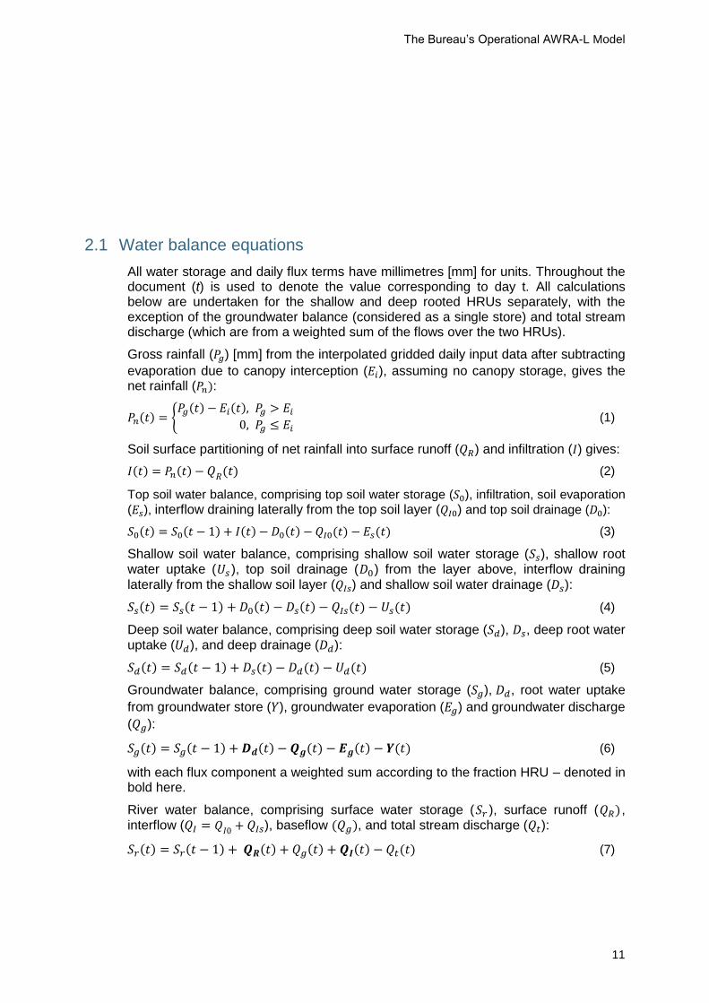
3.2.2 Upward longwave radiation
Upward longwave radiation 𝐿𝑢 [W/m2] is calculated according to black body theory
with the terrestrial surface radiation given as 휀𝜎𝑇4. Assuming a surface emissivity 휀 of 1 (Van Dijk, 2010c) and using the air temperature 𝑇𝑎 [°C] as an estimate of the surface temperature [°K] gives
𝐿𝑢(𝑡) = 𝜎(𝑇𝑎(𝑡) + 273.15)4
with 𝜎 [W/m2/K4] the Stefan-Boltzmann constant represented as 5.67x10⁻⁸ in the model (Dong et al., 1992; Donohue, McVicar and Roderick, 2009).
3.2.3 Downward longwave radiation
The downward longwave radiation 𝐿𝑑 [W/m2] is calculated from:
𝐿𝑑(𝑡) = 𝜎(𝑇𝑎(𝑡) + 273.15)4 {1 − [1 − 0.65 (𝑒𝑎(𝑡)
𝑇𝑎(𝑡) + 273.15)
0.14
] (1.35𝐾𝑑(𝑡)
𝐾𝑑0(𝐷𝑂𝑌)− 0.35)}
Where 𝐾𝑑0 is the expected downwelling shortwave radiation on a cloudless day (MJ m–2 d–1) as a function of the numeric day of the year (𝐷𝑂𝑌), latitude (𝜙) [radians],
solar declination 𝛿 [radians] and 𝜔 the sunset hour angle [radians]:
𝐾𝑑0(𝐷𝑂𝑌) =94.5 (1 + 0.033 cos(
2𝜋𝐷𝑂𝑌365
))
𝜋(𝜔 sin 𝛿 sin 𝜙 + cos 𝛿 cos 𝜙 sin 𝜔)
𝛿 = 0.006918 − 0.39912 cos(𝑄0) + 0.070257 sin(𝑄0)− 0.006758 cos(2𝑄0) + 0.000907 sin(2𝑄0)− 0.002697 cos(3𝑄0) + 0.00148 sin(3𝑄0)
𝑄0 = 2𝜋(𝐷𝑂𝑌 − 1)/365
This is similar to the equation for 𝐿𝑑 in Donohue et al. (2009), but with different parameterisations for the atmospheric emissivity and transmissivity for a clear sky. It is noted that this is different from the initial derivation provided by Van Dijk (2010c), as Downwelling longwave radiation is now augmented by radiation from the cloud base (see Viney et al, 2015). The derivation is detailed in Appendix B.

The Bureau’s Operational AWRA-L Model: Technical description of AWRA-L version 5
24
3.3 Actual evapotranspiration (𝐸𝑡𝑜𝑡)
Total actual evapotranspiration 𝐸𝑡𝑜𝑡 [mm] is the sum of evaporation (interception 𝐸𝑖, soil 𝐸𝑠 and groundwater 𝐸𝑔 ) and transpiration (shallow 𝑈𝑠 and deep 𝑈𝑑 root water
uptake, transpiration from groundwater 𝑌):
𝐸𝑡𝑜𝑡 = 𝐸𝑖 + 𝐸𝑠 + 𝐸𝑔 + 𝑈𝑠 + 𝑈𝑑 + 𝑌 (42)
each described below. It is noted that Canopy interception and transpiration from groundwater are not limited by the total sum being less than potential evaporation – hence total values greater than potential can occur on a given day.
3.3.1 Interception evaporation (𝑬𝒊)
The evaporation of intercepted rainfall (𝐸𝑖), following VanDijk (2010) is the widely adopted and evaluated event-based rainfall interception model of Gash (1979), with modifications made later by Gash, Lloyd and Lachaudb (1995) and Van Dijk and Bruijnzeel (2001) to allow application to vegetation with a sparse canopy.
𝐸𝑖(𝑡) = {𝑓𝑣(𝑡)𝑃𝑔(𝑡) 𝑖𝑓 𝑃𝑔(𝑡) < 𝑃𝑤𝑒𝑡(𝑡)
𝑓𝑣(𝑡)𝑃𝑤𝑒𝑡(𝑡) + 𝑓𝐸𝑅(𝑡) (𝑃𝑔(𝑡) − 𝑃𝑤𝑒𝑡(𝑡)) 𝑖𝑓 𝑃𝑔(𝑡) ≥ 𝑃𝑤𝑒𝑡(𝑡) (43)
where 𝑓𝑣 [-] is the fractional canopy cover (see Section 4 Vegetation Phenology), 𝑃𝑤𝑒𝑡 [mm] is the reference threshold rainfall amount at which the canopy is wet:
𝑃𝑤𝑒𝑡(𝑡) = − ln (1 −𝑓𝐸𝑅(𝑡)
𝑓𝑣(𝑡))
𝑆𝑣𝑒𝑔(𝑡)
𝑓𝐸𝑅(𝑡) (44)
For small rainfall events where 𝑃𝑔(𝑡) < 𝑃𝑤𝑒𝑡(𝑡), all rainfall that falls on the vegetated
part of the landscape is assumed to be intercepted. The energy required for evaporation of intercepted water is assumed independent of potential evaporation. It is further assumed that this energy does not reduce the available energy for the remaining evaporative fluxes.
The canopy rainfall storage capacity 𝑆𝑣𝑒𝑔 [mm] given by
𝑆𝑣𝑒𝑔(𝑡) = 𝑠𝑙𝑒𝑎𝑓 𝐿𝐴𝐼(𝑡) (45)
where the specific canopy rainfall storage capacity per unit leaf area 𝑠𝑙𝑒𝑎𝑓 [mm] is a
HRU specific calibration parameter. 𝐿𝐴𝐼 is the Leaf Area Index [-], the one-sided greenleaf area per unit ground surface area, that is directly related to 𝑓𝑣 (see Section 4).
The ratio of average evaporation rate to average rainfall intensity (during storms) 𝑓𝐸𝑅 [-] is:
𝑓𝐸𝑅(𝑡) = 𝐹𝐸𝑅0𝑓𝑣(𝑡) (46)
The Bureau’s Operational AWRA-L Model
25
where the specific ratio of average evaporation rate over average rainfall intensity during storms per unit canopy cover 𝐹𝐸𝑅0 [-] is a calibration parameter.
3.3.2 Soil evaporation (𝑬𝒔)
The evaporation from soil 𝐸𝒔 [mm] occurs from the unsaturated portion of the grid cell (1 − 𝑓𝑠𝑎𝑡), as a fraction of the potential evaporation (𝐸0) possible after shallow and deep (𝐸𝑡) rooted transpiration (described below) have been subtracted:
𝐸𝑠(𝑡) = (1 − 𝑓𝑠𝑎𝑡(𝑡))𝑓𝑠𝑜𝑖𝑙 𝐸(𝑡) [𝐸0(𝑡) − 𝐸𝑡(𝑡)] (47)
where the relative soil evaporation 𝑓𝑠𝑜𝑖𝑙 𝐸 [-] is
𝑓𝑠𝑜𝑖𝑙 𝐸(𝑡) = 𝑓𝑠𝑜𝑖𝑙 𝐸 𝑚𝑎𝑥 min (1,𝑤0(𝑡)
𝑤0 lim 𝐸) (48)
and 𝑓𝑠𝑜𝑖𝑙 𝐸 𝑚𝑎𝑥] is the relative soil evaporation when soil water supply is not limiting
and 𝑤⏞0 𝑙𝑖𝑚 𝐸 [-] is the relative top soil water content at which evaporation is reduced.
3.3.3 Evaporation from groundwater (𝑬𝒈)
The evaporation from groundwater 𝐸𝑔 [mm/day] occurs from the saturated portion of
the grid cell (𝑓𝑠𝑎𝑡), as a fraction of the potential evaporation (𝐸0) possible after shallow and deep (𝐸𝑡) rooted transpiration (described below) have been subtracted:
𝐸𝑔(𝑡) = 𝑓𝑠𝑎𝑡(𝑡)𝑓𝑠𝑜𝑖𝑙 𝐸 𝑚𝑎𝑥[𝐸0(𝑡) − 𝐸𝑡(𝑡)] (49)
where the same model as the evaporation from soil is used, with the top soil layer saturated (𝑤0(𝑡) = 1).
3.3.4 Root water uptake from (𝑬𝒕 = 𝑼𝒔 + 𝑼𝒅)
Total transpiration from plants 𝐸𝑡 [mm] in the shallow and deep soil stores is equivalent to the sum of root water uptake from the shallow and deep rooted vegetation. The transpiration fluxes are limited by two factors: a potential transpiration
rate 𝐸𝑡 𝑚𝑎𝑥 and a maximum root water uptake 𝑈0. The actual transpiration is then calculated as the lesser of the two and this amount is distributed among the potential
transpiration water sources. The overall transpiration rate given by 𝑈 is used in the estimation of 𝑈𝑠 and 𝑈𝑑 the shallow and deep rooted vegetation transpiration
respectively. As 𝑈𝑠 and 𝑈𝑑 may be limited by available soil water, an adjusted total transpiration rate is finally recalculated. This final value of 𝑬𝒕 is then used to reduce the energy available for direct evaporation.
The maximum root water uptake under ambient conditions 𝑈0 [mm/day] is simply the greater of the maximum root water uptake from the shallow soil store 𝑈𝑠 𝑚𝑎𝑥 [mm/day]
and the deep soil store 𝑈𝑑 𝑚𝑎𝑥 [mm/day]:

The Bureau’s Operational AWRA-L Model: Technical description of AWRA-L version 5
26
𝑈0(𝑡) = max[𝑈𝑠 𝑚𝑎𝑥(𝑡), 𝑈𝑑 𝑚𝑎𝑥(𝑡)] (50)
with the maximum root water uptake from the shallow soil store 𝑈𝑠 𝑚𝑎𝑥 [mm/day] given by:
𝑈𝑠 𝑚𝑎𝑥(𝑡) = 𝑈𝑠 𝑀𝐴𝑋 min (1,𝑤𝑠(𝑡)
𝑤𝑠 𝑙𝑖𝑚) (51)
with the physiological maximum root water uptake from the shallow soil store 𝑈𝑠 𝑀𝐴𝑋 [mm/day] a parameter that is fixed to 6 for both the deep and shallow rooted HRU based on site water use at flux towers (Van Dijk, 2010c). Similarly, the relative shallow soil water content at which transpiration is reduced 𝑤𝑠 𝑙𝑖𝑚] is fixed to 0.3 for both deep and shallow HRUs.
The maximum root water uptake from the deep soil store 𝑈𝑑 𝑚𝑎𝑥 [mm/day] is given by
𝑈𝑑 𝑚𝑎𝑥(𝑡) = 𝑈𝑑 𝑀𝐴𝑋 min (1,𝑤𝑑(𝑡)
𝑤𝑑 𝑙𝑖𝑚) (52)
with the physiological maximum root water uptake from the deep soil store 𝑈𝑑 𝑀𝐴𝑋 [mm/day] a parameter for the deep rooted HRU, and fixed to 0 for the shallow rooted HRU (that cannot access the deep soil store). Similarly, the relative deep soil water content at which transpiration is reduced 𝑤𝑑 𝑙𝑖𝑚], the value is fixed to 0.3 for both deep and shallow HRUs.
The root water uptake 𝑈 [mm/day] is simply the lesser of the maximum root water
uptake under ambient conditions 𝑈0 [mm/day] and the maximum transpiration 𝐸𝑡 𝑚𝑎𝑥 [mm/day]
𝑈(𝑡) = min[𝑈0(𝑡), 𝐸𝑡 𝑚𝑎𝑥(𝑡)] (53)
where the maximum transpiration 𝐸𝑡 𝑚𝑎𝑥 [mm/day] is given by
𝐸𝑡 𝑚𝑎𝑥(𝑡) = 𝑓𝑡(𝑡)𝐸0(𝑡) (54)
and the potential transpiration fraction 𝑓𝑡 [-] is given by
𝑓𝑡(𝑡) =1
1+(𝑘𝜀(𝑡)
1+𝑘𝜀(𝑡))
𝑔𝑎(𝑡)
𝑔𝑠(𝑡)
(55)
Where 𝑔𝑎 [m/s] is aerodynamic conductance, and 𝑔𝑠 [m/s] the canopy conductance,
and 𝑘𝜀 [-] is a coefficient that determines evaporation efficiency:
𝑘𝜀(𝑡) = ∆(𝑡) γ⁄
where ∆ [Pa/K] is the slope of the saturation vapour pressure curve, 𝑅𝑛 [MJ m–2 d–1]
net radiation, γ [Pa/K] the psychometric constant.
Aerodynamic conductance (𝑔𝑎) is given by:
𝑔𝑎(t) =0.305 𝑢2(𝑡)
ln(813
ℎ𝑣𝑒𝑔−5.45)(2.3+ln(
813
ℎ𝑣𝑒𝑔−5.45))
(56)

The Bureau’s Operational AWRA-L Model
27
Where ℎ𝑣𝑒𝑔 is the height of the vegetation canopy [m]. This equation was derived by
Van Dijk (2010c) based on the well-established theory proposed by Thom (1975). The derivation is provided in Appendix B.
The height of the top of the canopy (Figure 13) is derived from the global 1 km lidar estimates of Simard et al. (2011) and is assumed to be appropriate only for the deep-rooted HRU. For the shallow-rooted HRU, the vegetation height is optimisable, but is assumed to take a fixed value of 0.5 m. Vegetation height is assumed static throughout the simulation.
Canopy (surface) conductance 𝑔𝑠 [m/s] is given by:
𝑔𝑠(t) = 𝑓𝑣(𝑡)𝑐𝑔𝑠𝑚𝑎𝑥𝑉𝑐 (57)
where 𝑓𝑣 the fractional canopy cover is discussed in Section 4, 𝑐𝑔𝑠𝑚𝑎𝑥 is a coefficient
relating vegetation photosynthetic capacity to maximum stomatal conductance (m s–1), and 𝑉𝑐 is vegetation photosynthetic capacity index (per unit canopy cover) described in section 3.2 (Energy Balance). 𝑐𝑔𝑠𝑚𝑎𝑥 is currently optimised for both the shallow and
deep rooted HRUs, although Van Dijk (2010c) showed that an a priori estimate of 0.03 may be justified.
The root water uptake from the shallow soil store 𝑈𝑠 [mm/day] is given by:
𝑈𝑠(𝑡) = {min [𝑆𝑠(𝑡) − 0.01, (
𝑈𝑠 𝑚𝑎𝑥(𝑡)
𝑈𝑠 𝑚𝑎𝑥(𝑡)+𝑈𝑑 𝑚𝑎𝑥(𝑡)) 𝑈(𝑡)] 𝑖𝑓 𝑈0(𝑡) > 0
0 𝑖𝑓 𝑈0(𝑡) ≤ 0 (58)
The root water uptake from the deep soil store 𝑈𝑑 [mm/day] is given by:
𝑈𝑑(𝑡) = {min [𝑆𝑑(𝑡) − 0.01, (
𝑈𝑑 𝑚𝑎𝑥(𝑡)
𝑈𝑠 𝑚𝑎𝑥(𝑡)+𝑈𝑑 𝑚𝑎𝑥(𝑡)) 𝑈(𝑡)] 𝑖𝑓 𝑈0(𝑡) > 0
0 𝑖𝑓 𝑈0(𝑡) ≤ 0 (59)

The Bureau’s Operational AWRA-L Model: Technical description of AWRA-L version 5
28
Figure 13. Vegetation height of deep rooted vegetation (𝒉𝒗𝒆𝒈)
3.3.5 Transpiration from groundwater (𝒀)
Transpiration from the groundwater store (𝑌) [mm/day] is given by
𝑌(𝑡) = {(𝑓𝐸𝑔
(𝑡) − 𝑓𝑠𝑎𝑡(𝑡)) 𝑓𝑠𝑜𝑖𝑙 𝐸 𝑚𝑎𝑥[𝐸0(𝑡) − 𝐸𝑡(𝑡)] 𝑖𝑓 𝑓𝑠𝑎𝑡 < 𝑓𝐸𝑔
0 𝑖𝑓 𝑓𝑠𝑎𝑡 ≥ 𝑓𝐸𝑔
(60)
where 𝑓𝐸𝑔 [-] is the fraction of the landscape (grid cell) that is accessible for
transpiration from groundwater, and 𝑓𝑠𝑎𝑡 [-] is the fraction of the landscape (grid cell) that is saturated.

The Bureau’s Operational AWRA-L Model
29
Vegetation density plays a significant role in the water balance and streamflow generation. Some measure or estimate of vegetation density is therefore crucial for modulating the hydrological processes in AWRA-L.
In the case of AWRA-L leaf biomass 𝑀 [kg m–2] (directly related to leaf area index 𝐿𝐴𝐼 and fractional canopy cover 𝑓𝑣 – see below) modulates:
potential evaporation through alteration of albedo (within the energy balance)
interception through altering the area available for interception and also the rate of interception evaporation
transpiration through altering canopy conductance
A seasonal vegetation dynamics (or vegetation phenology) model is incorporated into AWRA-L to simulate vegetation cover dynamics in response to water availability. This is done under the assumption that the vegetation takes on the maximum density that could be sustained by the available moisture.
The ‘equilibrium’ leaf mass is estimated by considering the hypothetical leaf mass 𝑀𝑒𝑞 that corresponds with a situation in which maximum transpiration rate (𝐸𝑡 𝑚𝑎𝑥 –
Eqn 54) equals maximum root water uptake (𝑈0 – Eqn 50). The vegetation moves towards this equilibrium state with a prescribed degree of inertia, representative of alternative phenological strategies.
The seasonal vegetation dynamics model is constrained by the mass balance equation. Mass of vegetation 𝑀 [kg m–2] is given according:
𝑀(𝑡 + 1) = 𝑀(𝑡) + Δ𝑡𝑀𝑛(𝑡) (61)
where Δ𝑡 is the length of the time step [1 day], and 𝑀𝑛 is the change in leaf biomass at each time step [kg m–2 d–1] that moves towards the equilibrium leaf mass (𝑀𝑒𝑞:
defined further below) according to:
𝑀𝑛(𝑡) = {
𝑀𝑒𝑞(𝑡)−𝑀(𝑡)
𝑡𝑔𝑟𝑜𝑤, if 𝑀(𝑡) < 𝑀𝑒𝑞(𝑡)
𝑀𝑒𝑞(𝑡)−𝑀(𝑡)
𝑡𝑠𝑒𝑛𝑐, if 𝑀(𝑡) ≥ 𝑀𝑒𝑞(𝑡)
(62)
where 𝑡𝑔𝑟𝑜𝑤 [days] is the characteristic time scale for vegetation growth towards
equilibrium, 𝑡𝑠𝑒𝑛𝑐 [days] is the characteristic time scale for vegetation senescence towards equilibrium. There is little information available in the literature to estimate 𝑡𝑔𝑟𝑜𝑤 and 𝑡𝑠𝑒𝑛𝑐 from. However, they can readily be calibrated to LAI patterns derived
from remote sensing. Van Dijk (2010c) notes through visual estimation for around 30 sample locations across Australia, 𝑡𝑔𝑟𝑜𝑤and 𝑡𝑠𝑒𝑛𝑐 were both estimated at 50 days for
shallow-rooted vegetation, and 90 days for deep-rooted vegetation. However, 𝑡𝑔𝑟𝑜𝑤
values of 60 days and 10 days, and 𝑡𝑠𝑒𝑛𝑐 values of 1000 days and 150 days have been used subsequently for all version of the AWRA-L model.
4 Vegetation Phenology

The Bureau’s Operational AWRA-L Model: Technical description of AWRA-L version 5
30
This formulation was developed by Van Dijk (2010c) because literature review did not suggest a suitably simple model that predicts water-related vegetation phenology (see review by Arora (2002)). The formulation is based on the assumption that vegetation is able to adjust its leaf biomass at a rate that is independent of the amount of existing leaf biomass and energy or biomass embodied in other plant organs (a strong simplification of the complex physiological processes).
Fractional canopy cover 𝑓𝑣 [-], is related to biomass (𝑀) according to the following
dimensional conversion firstly to leaf area index 𝐿𝐴𝐼 [-] (the one-sided greenleaf area per unit ground surface area):
𝐿𝐴𝐼(𝑡) = 𝑀(𝑡) 𝑆𝐿𝐴 (63)
and then:
𝑓𝑣(𝑡) = 1 − exp (−𝐿𝐴𝐼(𝑡)
𝐿𝐴𝐼𝑟𝑒𝑓) (64)
where 𝑆𝐿𝐴 is the specific leaf area [m2 kg–1] (the ratio of leaf area to dry mass), and 𝐿𝐴𝐼𝑟𝑒𝑓 is the reference leaf are index [-] corresponding to 𝑓𝑣 = 0.63.
As Van Dijk (2010c) explains, the conversion from 𝐿𝐴𝐼 to 𝑓𝑣 is described by the exponential light extinction equation (Monsi and Saeki, 1953) equivalent to Beer’s Law which is most commonly used for this purpose. However to be consistent with notation elsewhere in the model, the so-called ‘light extinction coefficient’ (often
symbolised by κ) is not used but its inverse value 𝐿𝐴𝐼𝑟𝑒𝑓 , which represents a
reference LAI at which fraction cover is 0.632.
Globally reported values of 𝑆𝐿𝐴 vary by two orders of magnitude, from 0.7 to 71 m2 kg–1 (Wright et al., 2004). Values of 1.5 to 9 m2 kg–11 have been found for Australian Eucalypt species (Schulze et al., 2006) with an average value of of approximately 3 m2 kg–1. Fixed values of 10 m2 kg–1 and 3 m2 kg–1 were chosen by Van Dijk (2010c) for shallow and deep rooted vegetation HRUs respectively.
Maximum achievable canopy cover (𝑓𝑣𝑚𝑎𝑥) is given, inverting (61), by:
𝑓𝑣𝑚𝑎𝑥 = 1 − exp (−max (𝐿𝐴𝐼𝑚𝑎𝑥,0.00278
𝐿𝐴𝐼𝑟𝑒𝑓) (65)
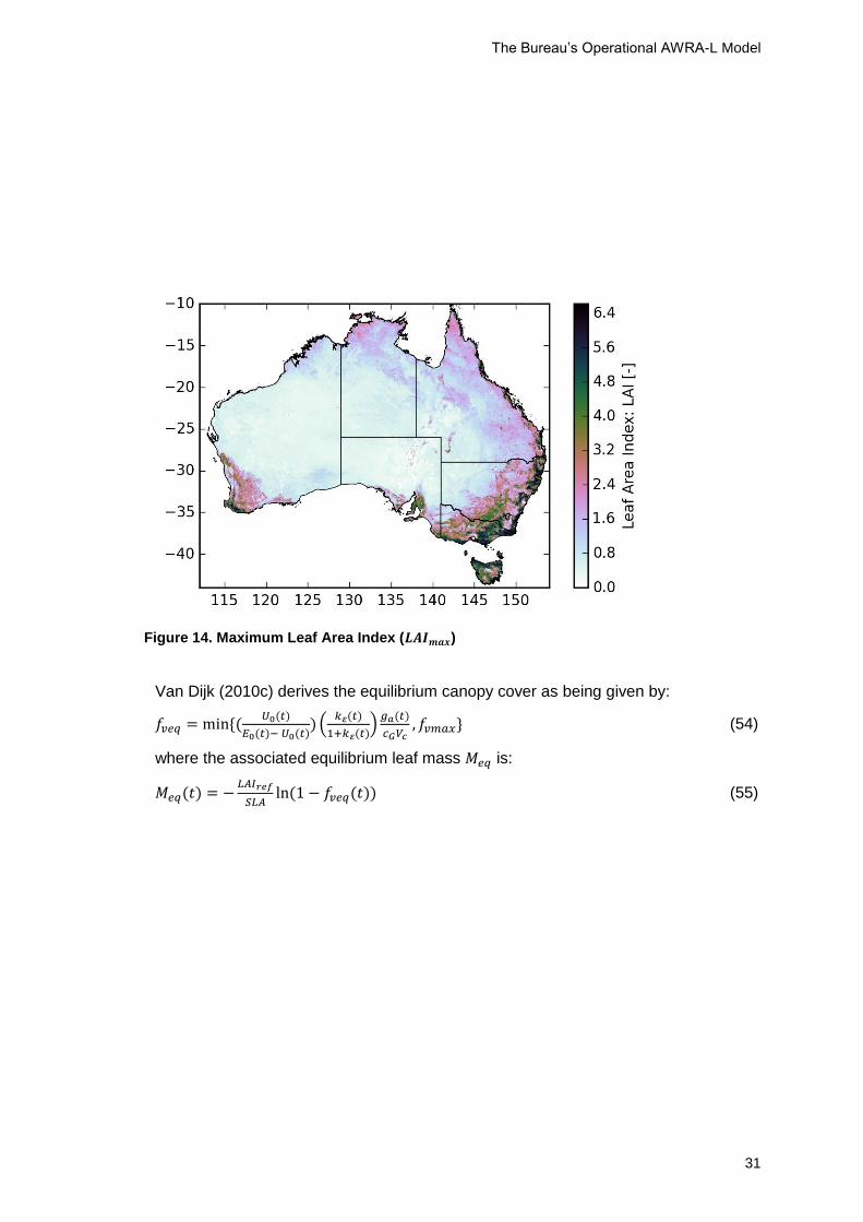
Where 𝐿𝐴𝐼𝑚𝑎𝑥 is the maximum achievable leaf area index [-]. 𝐿𝐴𝐼𝑚𝑎𝑥 is derived from a time series of LAI from the Moderate Resolution Imaging Spectroradiometer (MODIS) satellite (Figure 14). At present, the same values of 𝐿𝐴𝐼𝑚𝑎𝑥 are used for both HRUs.
The Bureau’s Operational AWRA-L Model
31
Figure 14. Maximum Leaf Area Index (𝑳𝑨𝑰𝒎𝒂𝒙)
Van Dijk (2010c) derives the equilibrium canopy cover as being given by:
𝑓𝑣𝑒𝑞 = min {(𝑈0(𝑡)
𝐸0(𝑡)− 𝑈0(𝑡)) (
𝑘𝜀(𝑡)
1+𝑘𝜀(𝑡))
𝑔𝑎(𝑡)
𝑐𝐺𝑉𝑐, 𝑓𝑣𝑚𝑎𝑥} (54)
where the associated equilibrium leaf mass 𝑀𝑒𝑞 is:
𝑀𝑒𝑞(𝑡) = −𝐿𝐴𝐼𝑟𝑒𝑓
𝑆𝐿𝐴ln(1 − 𝑓𝑣𝑒𝑞(𝑡)) (55)

The Bureau’s Operational AWRA-L Model: Technical description of AWRA-L version 5
32
AWRA-L v5.0 contains 49 notionally optimisable parameters – see Table 1. Twenty eight parameters are chosen a priori based through previous experience or according to mapping data – toward reducing the number of parameters to be optimised (and better identifying parameters that the model is sensitive to). The remaining 21 parameters chosen to be free, and are optimised across the continent to maximise a composite objective function combining the performance according to streamflow, ET and soil moisture at a set of 295 unimpaired catchments across Australia (see Figure 15).
The three datasets used in calibration over these catchments across Australia include:
Catchment streamflow: covering the period of 1981-2011. A set of 782 unimpaired catchments with gauged flow records in unimpaired across Australia were collated by Zhang et al. (2013) according to the following criteria: (a) catchment area is greater than 50 km2, (b) the stream is unregulated (no dams or reservoirs), (c) no major impacts of irrigation and land use, (d) observed record has at least 10 years of data between 1975 and 2011. The catchments (delineated using the Bureau’s national catchment Geofabric product: http://www.bom.gov.au/water/geofabric) were collated towards being used in evaluation. The spatial distribution of catchments reserved for calibration and validation of AWRA-L is shown in Figure 15; with regional divisions showing areas of similar climate. Data from 295 catchments covering the period 1/1/1981-30/12/2011 were used in calibration of AWRA-L while 291 catchments not used in calibration are used for validation.
Catchment evapotranspiration: CSIRO MODIS reflectance-based Scaling ET (CMRSET; Guerschman et al., 2009) - Satellite retrieval based grid estimates of evapotranspiration covering 2001-2010.
Catchment soil moisture: AMSR-E product (Owe, de Jeu and Holmes, 2008) - Satellite retrieval based grid estimates of soil moisture, covering the period of 2002-2011 have been used.
Various statistics are calculated for each catchment to assess the models performance during calibration:
Relative bias (B)
1
ti tii
i
T
o m
i
t o
Q QB
Q
(56)
Nash-Sutcliffe Efficiency (NSE)
5 Parameterisation

The Bureau’s Operational AWRA-L Model
33
2
1
2
1
1
i
ti ti
i
ti i
T
o m
t
i T
o o
t
Q Q
NSE
Q Q
(57)
Pearson's correlation coefficient (𝑟)
𝑟 =∑ (𝑄𝑜
𝑡𝑖−𝑄𝑜𝑖̅̅ ̅̅ )(𝑄𝑚
𝑡𝑖−𝑄𝑚𝑖̅̅ ̅̅ ̅)
𝑇𝑖𝑡=1
√∑ (𝑄𝑜𝑡𝑖−𝑄𝑜
𝑖̅̅ ̅̅ )2𝑇𝑖
𝑡=1√∑ (𝑄𝑚
𝑡𝑖−𝑄𝑚𝑖̅̅ ̅̅ ̅)
2𝑇𝑖𝑡=1
(58)
The following streamflow objective function is evaluated for each catchment simulation (as derived by Viney et al., 2009 with the addition of a monthly NSE term):
Fs = (NSEd + NSEm)/2 – 5 ln(1 + B) 2.5 (59)
where NSEd and NSEm are daily and monthly Nash-Sutcliffe Efficiency (Eq. 57) and
B is relative bias (B). Daily soil moisture correlation ( 𝑟𝑠𝑚 ) and monthly evapotranspiration ( 𝑟𝑒𝑡) (defined in Eq. 58) are also used for each catchment according to the weighted function:
F = 0.7 * Fs + 0.15 * 𝑟𝑠𝑚 + 0.15 *𝑟𝑒𝑡 (60)
Finally, the national calibration of AWRA-L maximises the grand objective function:
grandF =mean(F25%,F50%,F75%,F100%) (61)
where FX% is the Xth ranked site percentile F value. This objective function aims to get an adequate fit over a wide range of sites, but also to exclude very poor fitting areas (i.e. those below the 25%).
For further details of calibration, evaluation of model performance and a-priori specification of model parameters see Viney et al. (2015), Frost et al., (2016) and Van Dijk (2010c).

The Bureau’s Operational AWRA-L Model: Technical description of AWRA-L version 5
34
Table 1. List of AWRA-L parameter values. Values that apply to either the deep or shallow
rooted HRU (or both) are provided. Values that are optimised are shown in bold.
Symbol Definition Deep Shallow Unit
αd Dry soil albedo 0.26 0.26 -
αw Wet soil albedo 0.16 0.16 -
cG Conversion coefficient from vegetation photosynthetic capacity index to maximum stomatal conductance
0.0320 0.0237 m/s
fER Ratio of average evaporation rate over average rainfall intensity during storms per unit canopy cover
0.0736 0.5 -
Fsmax Soil evaporation scaling factor when soil water supply is not limiting evaporation
0.2275 0.9297 -
𝒉𝒗𝒆𝒈 Height of vegetation canopy Grid 0.5 m
LAIref Reference leaf area index (at which fv = 0.63) 2.5 1.4 -
SLA Specific leaf area 3 10 m2/kg
sl Specific canopy rainfall storage capacity per unit leaf area 0.0946 0.0427 mm
tgrow Characteristic time scale for vegetation growth towards equilibrium
1000 150 days
tsenc Characteristic time scale for vegetation senescence towards equilibrium
60 10 days
Us0 Maximum root water uptake rates from shallow soil store 0 6 mm/d
Ud0 Maximum root water uptake rates from deep soil store 7.1364 0 mm/d
Vc Vegetation photosynthetic capacity index per unit canopy cover
0.35 0.65 -
w0lim Relative top soil water content at which evaporation is reduced 0.85 0.85 -
wslim Water-limiting relative water content in shallow soil store 0.3 0.3 -
wdlim Water-limiting relative water content in deep soil store 0.3 0.3 -
DR Rooting depth 6 1 m
Kgw scale Multiplier on the raster input of Kgw 0.5022 -
Krint Intercept coefficient for calculating routing coefficient Kr 0.1577 -
Krscale Scale coefficient for calculating routing coefficient Kr 0.0508 -
kβ Coefficient on the mapped slope for the calculation of interflow 0.9518 -
kζ Coefficient on the ratio of Ksat across soil horizons for the calculation of interflow
0.0741 -
K0satscale Scale for saturated hydraulic conductivity in the surface layer 2.8728 -
Kssatscale Scale for saturated hydraulic conductivity in the shallow layer 0.0202 -
Kdsatscale Scale for saturated hydraulic conductivity in the deep layer 0.0100 -
nscale Scale for effective porosity 0.0552 -
Prefscale Multiplier on the raster input of Pref 1.8153 -
S0maxscale Scale for maximum water storage in the surface layer 2.9958 -
Ssmaxscale Scale for maximum water storage in the shallow layer 2.4333 -
Sdmaxscale Scale for maximum water storage in the deep layer 0.7951 -

The Bureau’s Operational AWRA-L Model
35
Figure 15. Location of unimpaired catchments used for model evaluation with climate zones overlain.

The Bureau’s Operational AWRA-L Model: Technical description of AWRA-L version 5
36
Allen, R. G., Pereira, L. S., Raes, D. and Smith, M. (1998) ‘Crop evapotranspiration: Guidelines for computing crop requirements’, Irrigation and Drainage Paper No. 56, FAO, (56), p. 300. doi: 10.1016/j.eja.2010.12.001.
Arora, V. (2002) ‘Modeling vegetation as a dynamic component in soil-vegetation-atmosphere transfer schemes and hydrological models’, Reviews of Geophysics, 40(2), pp. 1–26. doi: 10.1029/2001RG000103.
Brunt, D. (1932) ‘Notes on radiation in the atmosphere. I’, Quarterly Journal of the Royal Meteorological Society, 58(247), pp. 389–420. doi: 10.1002/qj.49705824704.
Brutsaert, W. (1975) ‘On a derivable formula for long-wave radiation from clear skies’, Water Resources Research, 11(5), pp. 742–744. doi: 10.1029/WR011i005p00742.
Dane, J. H. and Puckett, W. (1994) ‘Field soil hydraulic properties based on physical and mineralogical information’, in al., Mt. van G. et (ed.) International Workshop on Indirect Methods for Estimating the Hydraulic Properties of Unsaturated Soils. Riverside, CA: University of California, pp. 389–403.
Dong, A., Grattan, S. R., Carroll, J. J. and Prashar, C. R. K. (1992) ‘Estimation of Daytime Net Radiation Over Well Watered Grass’, Journal of Irrigation and Drainage Engineering, 118(3), pp. 466–479. doi: 10.1061/(ASCE)0733-9437(1992)118:3(466).
Donohue, R. J., Mcvicar, T. R. and Roderick, M. L. (2009) Generating Australian potential evaporation data suitable for assessing the dynamics in evaporative demand within a changing climate. CSIRO: Water for a Healthy Country National Research Flagship.
Donohue, R. J., Roderick, M. L. and McVicar, T. R. (2008) ‘Deriving consistent long-term vegetation information from AVHRR reflectance data using a cover-triangle-based framework’, Remote Sensing of Environment, 112(6), pp. 2938–2949. doi: http://dx.doi.org/10.1016/j.rse.2008.02.008.
Duffie, J. A. and Beckman, W. A. (2013) Solar Engineering of Thermal Processes Solar Engineering. 4th edn. Hoboken, New Jersey: Wiley.
Elmahdi, A., Hafeez, M., Smith, A., Frost, A., Vaze, J. and Dutta, D. (2015) ‘Australian Water Resources Assessment Modelling System (AWRAMS)-informing water resources assessment and national water accounting’, 36th Hydrology and Water Resources Symposium: The art and science of water. Barton, ACT: Engineers Australia, pp. 979–986.
Fröhlich, C. and Brusa, R. W. (1981) ‘Solar radiation and its variation in time’, Solar Physics, 74, pp. 209–215. doi: 10.1017/CBO9781107415324.004.
References

The Bureau’s Operational AWRA-L Model
37
Frost, A. J., Ramchurn, A. and Hafeez, M. (2016) Evaluation of the Bureau’s Operational AWRA-L Model. Bureau of Meteorology Techical Report.
Gash, J. H. C. (1979) ‘An analytical model of rainfall interception by forests’, Quarterly Journal of the Royal Meteorological Society, 105(443), pp. 43–55. doi: 10.1002/qj.49710544304.
Gash, J. H. C., Lloyd, C. R. and Lachaudb, G. (1995) ‘Estimating sparse forest rainfall interception with an analytical model’, Journal of Hydrology, 170(95), pp. 79–86. doi: 10.1016/0022-1694(95)02697-N.
Grant, I., Jones, D., Wang, W., Fawcett, R. and Barratt, D. (2008) ‘Meteorological and remotely sensed datasets for hydrological modelling: a contribution to the Australian Water Availability Project’, in Proceedings of the Catchment-scale Hydrological Modelling & Data Assimilation (CAHMDA-3) International Workshop on Hydrological Prediction: Modelling, Observation and Data Assimilation, January 9 2008–January 11 2008.
Guerschman, J. P., Van Dijk, A. I. J. M., Mattersdorf, G., Beringer, J., Hutley, L. B., Leuning, R., Pipunic, R. C. and Sherman, B. S. (2009) ‘Scaling of potential evapotranspiration with MODIS data reproduces flux observations and catchment water balance observations across Australia’, Journal of Hydrology, 369(1–2), pp. 107–119. Available at: http://www.sciencedirect.com/science/article/B6V6C-4VMGV01-1/2/45782648e306eb0ef4352384e77d228a.
Hafeez, M., Smith, A., Frost, A., Srikanthan, S., Elmahdi, A., Vaze, J. and Prosser, I. (2015) ‘The Bureau’s Operational AWRA Modelling System in the context of Australian landscape and hydrological model products’, 36th Hydrology and Water Resources Symposium. Hobart, Australia: Engineers Australia, (December).
Iqbal, M. (1983) An Introduction to Solar Radiation.
Jensen, M. E., Wright, J. L. and Pratt, B. J. (1971) ‘Estimating Soil Moisture Depletion from Climate, Crop and Soil Data’, Transaction of the ASAE, 14(5), pp. 954–959.
Johnston, R. M., Barry, S. J., Bleys, E., Bui, E. N., Moran, C. J., Simon, D. A. P., Carlile, P., McKenzie, N. J., Henderson, B. L., Chapman, G., Imhoff, M., Maschmedt, D., Howe, D., Grose, C., Schoknecht, N., Powell, B. and Grundy, M. (2003) ‘ASRIS: the database’, Soil Research, 41(6), pp. 1021–1036. doi: http://dx.doi.org/10.1071/SR02033.
Jones, D. A., Wang, W. and Fawcett, R. (2009) ‘High-quality spatial climate data-sets for Australia’, Australian Meteorological and Oceanographic Journal, 58, pp. 233–248.
Liu, B. Y. H. and Jordan, R. C. (1960) ‘The interrelationship and characteristic

The Bureau’s Operational AWRA-L Model: Technical description of AWRA-L version 5
38
distribution of direct, diffuse and total solar radiation’, Solar Energy, 4(3), pp. 1–19. doi: 10.1016/0038-092X(60)90062-1.
McVicar, T. R., Van Niel, T. G., Li, L. T., Roderick, M. L., Rayner, D. P., Ricciardulli, L. and Donohue, R. J. (2008) ‘Wind speed climatology and trends for Australia, 1975-2006: Capturing the stilling phenomenon and comparison with near-surface reanalysis output’, Geophysical Research Letters, 35(L20403). doi: 10.1029/2008GL035627.
Monsi, M. and Saeki, T. (1953) ‘Über den Lichtfaktor in den Pflanzengesellschaften und seine Bedeutung für die Stoffproduktion’, Japanese Journal of Botany, 14, pp. 22–52. doi: 10.1093/aob/mci052.
Owe, M., de Jeu, R. and Holmes, T. (2008) ‘Multisensor historical climatology of satellite-derived global land surface moisture’, Journal of Geophysical Research: Earth Surface, 113(F1), p. F01002. doi: 10.1029/2007jf000769.
Peeters, L. J. M., Crosbie, R. S., Doble, R. C. and Van Dijk, A. I. J. M. (2013) ‘Conceptual evaluation of continental land-surface model behaviour’, Environmental Modelling & Software, 43(0), pp. 49–59. doi: http://dx.doi.org/10.1016/j.envsoft.2013.01.007.
Penman, H. L. (1948) ‘Natural Evporation from Open Water, Bare Soil and Grass’, The Royal Society, 193(1032), pp. 120–145. doi: 10.1098/rspa.1948.0037.
Raupach, M. R., Briggs, P. R., Haverd, V., King, E. A., Paget, M. and Trudinger, C. M. (2008) Australian Water Availability Project (AWAP) - CSIRO Marine and Atmospheric Research Component: Final Report for Phase 3. Caberra, Australia: CSIRO Marine and Atmospheric Research.
Roderick, M. L. (1999) ‘Estimating the diffuse component from daily and monthly measurements of global radiation’, Agricultural and Forest Meteorology, 95(3), pp. 169–185. doi: 10.1016/S0168-1923(99)00028-3.
Schulze, E. D., Turner, N. C., Nicolle, D. and Schumacher, J. (2006) ‘Species differences in carbon isotope ratios, specific leaf area and nitrogen concentrations in leaves of Eucalyptus growing in a common garden compared with along an aridity gradient’, Physiologia Plantarum, 127(3), pp. 434–444. doi: 10.1111/j.1399-3054.2006.00682.x.
Shuttleworth, W. J. (1992) ‘Chapter 4. Evaporation’, in Maidment, D. R. (ed.) ‘Handbook of Hydrology’, p. 4.1-4.53.
Simard, M., Pinto, N., Fisher, J. B. and Baccini, A. (2011) ‘Mapping forest canopy height globally with spaceborne lidar’, Journal of Geophysical Research: Biogeosciences, 116(G4), p. G04021. doi: 10.1029/2011jg001708.
Spencer, J. W. (1971) ‘Fourier series representation of the position of the Sun’, Search, 2(5), p. 172.
The Bureau’s Operational AWRA-L Model
39
Thom, A. . (1975) ‘3. Momentum, Mass and Heat Exchange of Plant Communities’, in Vegetation and the atmosphere: principles, p. 57.
Van Dijk, A. I. J. M. (2010a) ‘Climate and terrain factors explaining streamflow response and recession in Australian catchments’, Hydrology and Earth System Sciences. Copernicus GmbH, 14(1), pp. 159–169. doi: 10.5194/hess-14-159-2010.
Van Dijk, A. I. J. M. (2010b) ‘Selection of an appropriately simple storm runoff model’, Hydrology and Earth System Sciences. Copernicus GmbH, 14(3), pp. 447–458. doi: 10.5194/hess-14-447-2010.
Van Dijk, A. I. J. M. (2010c) The Australian Water Resources Assessment System. Technical Report 3. Landscape Model (version 0.5) Technical Description. Report. CSIRO: Water for a Healthy Country National Research Flagship.
Van Dijk, A. I. J. M. and Bruijnzeel, L. A. (2001) ‘Modelling rainfall interception by vegetation of variable density using an adapted analytical model. Part 1. Model description’, Journal of Hydrology, 247(3–4), pp. 230–238. doi: 10.1016/S0022-1694(01)00392-4.
Vaze, J., Viney, N., Stenson, M., Renzullo, L., Van Dijk, A., Dutta, D., Crosbie, R., Lerat, J., Penton, D., Vleeshouwer, J., Peeters, L., Teng, J., Kim, S., Hughes, J., Dawes, W., Zhang, Y., Leighton, B., Perraud, J., Joehnk, K., Yang, A., Wang, B., Frost, A., Elmahdi, A., Smith, A. and Daamen, C. (2013) ‘The Australian Water Resource Assessment System (AWRA)’, in Proceedings of the 20th International Congress on Modelling and Simulation. Adelaide, Australia.
Viney, N.R., Perraud, J., Vaze, J., Chiew, F.H.S., Post, D.A. and Yang, A. (2009) 'The usefulness of bias constraints in model calibration for regionalisation to ungauged catchments.' In: R.S. Anderssen, R.D. Braddock and L.T.H. Newham (Editors), 18th World IMACS / MODSIM Congress. Modelling and Simulation Society of Australia and New Zealand and International Association for Mathematics and Computers in Simulation, Cairns, Australia, pp. 3421-3427, http://www.mssanz.org.au/modsim09/I7/viney_I7a.pdf.
Viney, N. R., Vaze, J., Vleeshouwer, J., Yang, A., van Dijk, A. and Frost, A. (2014) ‘The AWRA modelling system’, Hydrology and Water Resources Symposium 2014. Perth: Engineers Australia, pp. 1018–1025. Available at: http://search.informit.com.au/documentSummary;dn=388600432195626;res=IELENG.
Viney, N., Vaze, J., Crosbie, R., Wang, B., Dawes, W. and Frost, A. (2015) AWRA-L v5.0: technical description of model algorithms and inputs. Report. CSIRO, Australia.
Wright, I. J., Westoby, M., Reich, P. B., Oleksyn, J., Ackerly, D. D., Baruch, Z.,
The Bureau’s Operational AWRA-L Model: Technical description of AWRA-L version 5
40
Bongers, F., Cavender-Bares, J., Chapin, T., Cornellissen, J. H. C., Diemer, M., Flexas, J., Gulias, J., Garnier, E., Navas, M. L., Roumet, C., Groom, P. K., Lamont, B. B., Hikosaka, K., Lee, T., Lee, W., Lusk, C., Midgley, J. J., Niinemets, Ü., Osada, H., Poorter, H., Pool, P., Veneklaas, E. J., Prior, L., Pyankov, V. I., Thomas, S. C., Tjoelker, M. G. and Villar, R. (2004) ‘The worldwide leaf economics spectrum’, Nature, 428, pp. 821–827. doi: 10.1038/nature02403.
Wright, J. L. (1982) ‘New Evapotranspiration Crop Coefficients’, Journal of the Irrigation and Drainage Division, 108(1), pp. 57–74.
Wright, J. L. and Jensen, M. E. (1972) ‘Peak Water Requirements of Crops in Southern Idaho’, Journal of the Irrigation and Drainage Division, 98(IR2), pp. 193–201.
Zhang, Y. Q., Viney, N., Frost, A., Oke, A., Brooks, M., Chen, Y. and Campbell, N. (2013) Collation of streamflow and catchment attribute dataset for 780 unregulated Australian catchments. Report. CSIRO: Water for a Healthy Country National Research Flagship.

The Bureau’s Operational AWRA-L Model
41
Appendix A: Table of model variables
Appendix B: Downward longwave radiation derivation
Appendices

The Bureau’s Operational AWRA-L Model: Technical description of AWRA-L version 5
42
Table 2. List of variable names used in this document and the corresponding variables used in the model code. Units are those given in this document.
Document Model code Description
𝜶 alb Surface albedo (dimensionless)
αdry alb_dry Dry soil albedo (dimensionless)
αs alb_soil Albedo of soil surface (dimensionless)
α alb_veg Albedo of vegetated surfaces (dimensionless)
αwet alb_wet Wet soil albedo (dimensionless)
β slope Slope of the land surface (percent)
γ gamma Psychrometric constant (Pa K–1
)
Δ delta Slope of the saturation vapour pressure curve (Pa K–1
)
DELTA Solar declination (radians)
λ lambda Latent heat of vaporisation (MJ kg–1
)
λd Dd Surface water drainage density (m–1
)
ρ0 Rh_0s Partitioning factor for vertical and lateral drainage from the surface soil layer (dimensionless)
ρs Rh_sd Partitioning factor for vertical and lateral drainage from the shallow soil layer (dimensionless)
σ StefBolz Stefan-Boltzmann constant (MJ m–2
d–1
K–4
)
latitude Latitude (radians), and is negative in the southern hemisphere
ω PI Sunset hour angle (radians)
𝒄𝒈𝒔𝒎𝒂𝒙 cGsmax Coefficient relating vegetation photosynthetic capacity to maximum stomatal conductance (m s
–1)
D0 D0 Vertical drainage from the bottom of the surface soil layer (mm)
Dd Dd Vertical drainage from the bottom of the deep soil layer (mm)
DR RD Rooting depth (m)
Ds Ds Vertical drainage from the bottom of the shallow soil layer (mm)
𝑫𝑶𝒀 DayOfYear Day of the year (d)
d0 — Depth of the top soil layer (mm)
dd — Depth of the deep soil layer (mm)
ds — Depth of the shallow soil layer (mm)
du — Depth of the unconfined aquifer (m)
E0 E0 Potential evaporation (mm d–1
)
𝑬∗ meanpet Long term mean daily potential evaporation (mm d–1
)
Es Es Evaporation flux from the surface soil store (mm d–1
)
Eg Eg Evaporation flux from the groundwater store (mm d–1
)
Ei Ei Evaporation flux from canopy interception (mm d–1
)
Et Et Actual total transpiration flux (mm d–1
)
Et max Etmax Potential transpiration rate (mm d–1
)
Etot Etot Total evapotranspiration (mm d–1
)
FER0 ER_frac_ref Specific ratio of the mean evaporation rate and the mean rainfall intensity during storms (dimensionless) fsoil E fsoile Relative soil evaporation
fsoil E max fsoilemax Soil evaporation scaling factor corresponding to unlimited soil water supply (dimensionless)
fEg fEgt Fraction of the grid cell that is accessible for transpiration from groundwater (dimensionless)
fer fer ratio of average evaporation rate to average rainfall intensity (during storms)
fsat fsat Fraction of the grid cell that is saturated at the surface (dimensionless)
ftree f_tree Fraction of tree cover within each grid cell (dimensionless)
fv fveg Fractional canopy cover (dimensionless)
fveq fveq Equilibrium canopy cover (dimensionless)
fPAR — Photosynthetically-active radiation (dimensionless)
ga ga Aerodynamic conductance (m s–1
)
Appendix A: Table of model variables
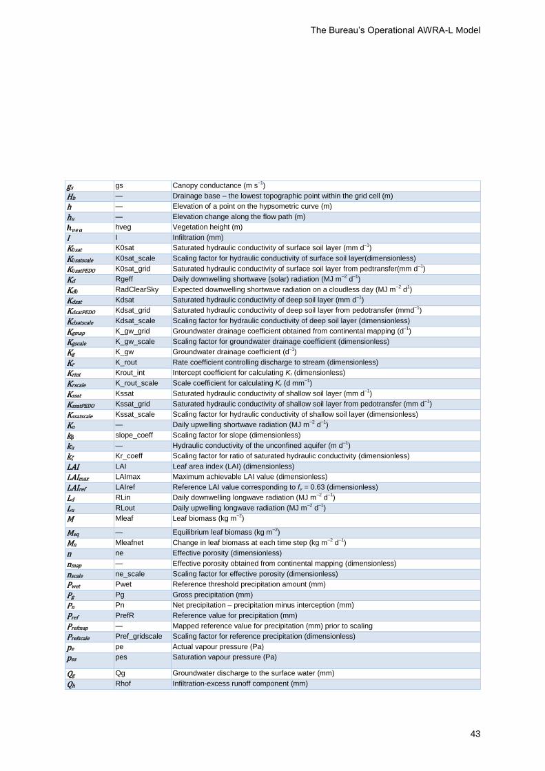
The Bureau’s Operational AWRA-L Model
43
gs gs Canopy conductance (m s–1
)
Hb — Drainage base – the lowest topographic point within the grid cell (m)
h — Elevation of a point on the hypsometric curve (m)
hu — Elevation change along the flow path (m)
𝒉𝒗𝒆𝒈 hveg Vegetation height (m)
I I Infiltration (mm)
K0sat K0sat Saturated hydraulic conductivity of surface soil layer (mm d–1
)
K0satscale K0sat_scale Scaling factor for hydraulic conductivity of surface soil layer(dimensionless)
K0satPEDO K0sat_grid Saturated hydraulic conductivity of surface soil layer from pedtransfer(mm d–1
)
Kd Rgeff Daily downwelling shortwave (solar) radiation (MJ m–2
d–1
)
Kd0 RadClearSky Expected downwelling shortwave radiation on a cloudless day (MJ m–2
d1)
Kdsat Kdsat Saturated hydraulic conductivity of deep soil layer (mm d–1
)
KdsatPEDO Kdsat_grid Saturated hydraulic conductivity of deep soil layer from pedotransfer (mmd–1
)
Kdsatscale Kdsat_scale Scaling factor for hydraulic conductivity of deep soil layer (dimensionless)
Kgmap K_gw_grid Groundwater drainage coefficient obtained from continental mapping (d–1
)
Kgscale K_gw_scale Scaling factor for groundwater drainage coefficient (dimensionless)
Kg K_gw Groundwater drainage coefficient (d–1
)
Kr K_rout Rate coefficient controlling discharge to stream (dimensionless)
Krint Krout_int Intercept coefficient for calculating Kr (dimensionless)
Krscale K_rout_scale Scale coefficient for calculating Kr (d mm–1
)
Kssat Kssat Saturated hydraulic conductivity of shallow soil layer (mm d–1
)
KssatPEDO Kssat_grid Saturated hydraulic conductivity of shallow soil layer from pedotransfer (mm d–1
)
Kssatscale Kssat_scale Scaling factor for hydraulic conductivity of shallow soil layer (dimensionless)
Ku — Daily upwelling shortwave radiation (MJ m–2
d–1
)
kβ slope_coeff Scaling factor for slope (dimensionless)
ku — Hydraulic conductivity of the unconfined aquifer (m d–1
)
kζ Kr_coeff Scaling factor for ratio of saturated hydraulic conductivity (dimensionless)
LAI LAI Leaf area index (LAI) (dimensionless)
LAImax LAImax Maximum achievable LAI value (dimensionless)
LAIref LAIref Reference LAI value corresponding to fv = 0.63 (dimensionless)
Ld RLin Daily downwelling longwave radiation (MJ m–2
d–1
)
Lu RLout Daily upwelling longwave radiation (MJ m–2
d–1
)
M Mleaf Leaf biomass (kg m–2
)
Meq — Equilibrium leaf biomass (kg m–2
)
Mn Mleafnet Change in leaf biomass at each time step (kg m–2
d–1
)
n ne Effective porosity (dimensionless)
nmap — Effective porosity obtained from continental mapping (dimensionless)
nscale ne_scale Scaling factor for effective porosity (dimensionless)
Pwet Pwet Reference threshold precipitation amount (mm)
Pg Pg Gross precipitation (mm)
Pn Pn Net precipitation – precipitation minus interception (mm)
Pref PrefR Reference value for precipitation (mm)
Prefmap — Mapped reference value for precipitation (mm) prior to scaling
Prefscale Pref_gridscale Scaling factor for reference precipitation (dimensionless)
pe pe Actual vapour pressure (Pa)
pes pes Saturation vapour pressure (Pa)
Qg Qg Groundwater discharge to the surface water (mm)
Qh Rhof Infiltration-excess runoff component (mm)

The Bureau’s Operational AWRA-L Model: Technical description of AWRA-L version 5
44
QIF QIF Interflow (mm)
QI0 IF0 Interflow draining laterally from the surface soil layer (mm)
QIs IFs Interflow draining laterally from the shallow soil layer (mm)
QR QR Surface runoff (mm)
Qs Rsof Saturation-excess runoff component (mm)
Qt Qtot Total discharge to stream (mm)
Rn Rneff Daily net radiation (MJ m–2
d–1
)
SLA SLA Specific leaf area (m2 kg
–1)
S0 S0 Water storage in the surface soil layer (mm)
S0AWC S0fracAWC_grid Available water holding capacity in the surface soil (dimensionless)
S0max S0max Maximum storage of the surface soil layer (mm)
S0maxscale S0max_scale Scaling parameter for maximum storage of the surface soil layer(dimensionless)
Sd Sd Water content of the deep soil store (mm)
Sdmax Sdmax Maximum storage of the deep soil layer (mm)
Sdmaxscale Sdmax_scale Scaling parameter for maximum storage of the deep soil layer(dimensionless)
Sg Sg Groundwater storage in the unconfined aquifer (mm)
Sr Sr Volume of water in the surface water store (mm)
Ss Ss Water content of the shallow soil store (mm)
SsAWC SsfracAWC_grid Available water holding capacity in the shallow soil (dimensionless)
Ssmax Ssmax Maximum storage of the shallow soil layer (mm)
Ssmaxscale Ssmax_scale Scaling parameter for maximum storage of the shallow soil layer (dimensionless)
sleaf S_sls Specific canopy rainfall storage per unit leaf area (mm)
Sveg sveg Canopy rainfall storage capacity (mm)
T - Surface temperature (K)
Ta Ta Daily mean temperature (°C)
Tmax Tmax Maximum air temperature (°C)
Tmin Tmin Minimum air temperature (°C)
t — Time step (d)
Δt — Length of the time step (d)
tgrow Tgrow Characteristic time scale for vegetation growth towards equilibrium (d)
tsenc Tsenc Characteristic time scale for vegetation senescence towards equilibrium(d)
U 0 U0 Maximum root water uptake (mm d–1
)
Ud Ud Root water uptake (transpiration) from the deep soil store (mm d–1
)
UdMAX Ud0 Maximum possible root water uptake from the deep soil store (mm d–1
)
Udmax Udmax Maximum root water uptake from the deep soil store at prevailing moisture content (mm d–1
)
Us Us Root water uptake (transpiration) from the shallow soil store (mm d–1
)
UsMAX Us0 Maximum possible root water uptake from the shallow soil store (mm d–1
)
Usmax Usmax Maximum root water uptake from the shallow soil store at prevailing moisture content (mm d–1
)
u2 u2 Wind speed at a height of 2 m (m s –1
)
Vc Vc Vegetation photosynthetic capacity per unit canopy cover
w0 w0 Relative soil moisture content of the top soil layer (dimensionless)
w0lim E w0limE Limiting the value of w0 at which evaporation is reduced (dimensionless)
w0ref w0ref_alb Reference value of w0 that determines the rate of albedo decrease with wetness (dimensionless) wd wd Relative water content of the deep soil store (dimensionless)
wdlim wdlimU Water-limiting relative water content of the deep soil store(dimensionless)
ws ws Relative water content of the shallow soil store(dimensionless)
wslim wslimU Water-limiting relative water content of the shallow soil store(dimensionless)
Y Y Root water uptake (transpiration) from the groundwater store (mm d–1
)

The Bureau’s Operational AWRA-L Model
45
The downward longwave radiation 𝐿𝑑 [W/m2] is derived from the net incoming
longwave radiation 𝑅𝑙𝑛 𝑖𝑛 [W/m2] and the upward longwave radiation 𝐿𝑢 [W/m2] as (Shuttleworth, 1992)
𝑅𝑙𝑛 𝑖𝑛(𝑡) = 𝐿𝑑(𝑡) − 𝐿𝑢(𝑡) (62)
with net outgoing longwave radiation 𝑅𝑙𝑛 𝑜𝑢𝑡 [W/m2], a negative flux (as 𝐿𝑢 > 𝐿𝑑 ), given by
𝑅𝑙𝑛 𝑜𝑢𝑡(𝑡) = −𝑅𝑙𝑛 𝑖𝑛(𝑡) (63)
Therefore, downward longwave radiation 𝐿𝑑 [W/m2] is given as
𝐿𝑑(𝑡) = 𝐿𝑢(𝑡) − 𝑅𝑙𝑛 𝑜𝑢𝑡(𝑡) (64)
with net outgoing longwave radiation 𝑅𝑙𝑛 𝑜𝑢𝑡 [W/m2] given by (Jensen, Wright and Pratt, 1971; Wright and Jensen, 1972; Wright, 1982; Shuttleworth, 1992; Allen et al., 1998)
𝑅𝑙𝑛 𝑜𝑢𝑡(𝑡) = 𝑓(𝑡)𝑅𝑙𝑛0 𝑜𝑢𝑡(𝑡) (65)
where the net outgoing longwave radiation for a clear sky 𝑅𝑙𝑛0 𝑜𝑢𝑡 [W/m2] is given by (Brunt, 1932; Jensen, Wright and Pratt, 1971; Wright and Jensen, 1972; Wright, 1982; Allen et al., 1998)
𝑅𝑙𝑛0 𝑜𝑢𝑡(𝑡) = (1 − 휀𝑎0(𝑡))𝜎(𝑇𝑎(𝑡) + 273.15)4 (66)
Where the surface emissivity 𝜺 is assumed 1, and 𝜺𝒂𝟎 [-] is the atmospheric emissivity
for a clear sky (Brutsaert, 1975) calculated from actual vapour pressure 𝑒𝑎 [mbar] and daytime air temperature [°K]
휀𝑎0(𝑡) = 1.24 (𝑒𝑎(𝑡)
𝑇𝑎(𝑡))
1
7 (67)
Or equivalently (with some truncation) after the units of vapour pressure 𝑒𝑎 [Pa] and daytime air temperature [°C] have been changed.
휀𝑎0(𝑡) = 0.65 (𝑒𝑎(𝑡)
𝑇𝑎(𝑡)+273.15)
0.14 (68)
And 𝑓 (-) is a cloudiness factor (Jensen, Wright and Pratt, 1971; Wright and Jensen, 1972; Wright, 1982; Shuttleworth, 1992; Allen et al., 1998)
𝑓(𝑡) = 1.35𝐾𝑑(𝑡)
𝐾𝑑0(𝐷𝑂𝑌)− 0.35 (69)
with 𝐷𝑂𝑌 [-] the numeric day of the year
With 𝐾𝑑 [MJ/m2/day] downward shortwave radiation, and 𝐾𝑑0 [MJ/m2/day] downward shortwave radiation for a clear sky, given as (Liu and Jordan, 1960; Dong et al., 1992; Donohue, Mcvicar and Roderick, 2009):
Appendix B: Downward longwave radiation derivation

The Bureau’s Operational AWRA-L Model: Technical description of AWRA-L version 5
46
𝐾𝑑0(𝐷𝑂𝑌) = 𝜏0𝑅𝑎(𝐷𝑂𝑌) (70)
where 𝑅𝑎 (MJ/m2/day) is extraterrestrial radiation, and the atmospheric transmissivity
for a clear sky 𝜏0 (-) for the southern hemisphere is (Roderick, 1999)
𝜏0 = 0.8 (71)
while a value of 0.7-0.75 could be used for the northern hemisphere (Roderick, 1999).
The extraterrestrial radiation 𝑅𝑎 [MJ/m2/day] is given by (Liu and Jordan, 1960; Iqbal, 1983; Shuttleworth, 1992; Allen et al., 1998; Duffie and Beckman, 2013)
𝑅𝑎(𝐷𝑂𝑌) =
24
𝜋𝐼𝑆𝐶𝐸0(𝐷𝑂𝑌)(𝜔(𝐷𝑂𝑌) sin 𝜙 sin 𝛿(𝐷𝑂𝑌) + cos 𝜙 cos 𝛿 (𝐷𝑂𝑌) sin 𝜔(𝐷𝑂𝑌)) (72)
where 𝐼𝑆𝐶 [kJ/m2/h] is the solar constant (4921 kJ/m2/h or 1367 W/m2) (Fröhlich and
Brusa, 1981; Iqbal, 1983) and 𝐸0 (-) is the eccentricity correction factor of the Earth’s orbit (around the sun) (Iqbal, 1983; Allen et al., 1998; Duffie and Beckman, 2013)
𝐸0(𝐷𝑂𝑌) = 1 + 0.033 cos (2𝜋𝐷𝑂𝑌
365) (73)
Substituting the values for the atmospheric transmissivity for a clear sky 𝜏0 (-) and the
solar constant 𝐼𝑆𝐶 [kJ/m2/h] gives
𝐾𝑑0(𝐷𝑂𝑌) =94.5
𝜋𝐸0(𝐷𝑂𝑌)(𝜔(𝐷𝑂𝑌) sin 𝛿(𝐷𝑂𝑌) sin 𝜙 + cos 𝛿 (𝐷𝑂𝑌) cos 𝜙 sin 𝜔(𝐷𝑂𝑌)) (74)
where 𝝎 [radians] is sunset hour (Liu and Jordan, 1960; Iqbal, 1983; Shuttleworth, 1992; Allen et al., 1998), given by
𝜔(𝐷𝑂𝑌) = cos−1(− tan 𝜙 tan 𝛿(𝐷𝑂𝑌)) (75)
with 𝝓 [radians] latitude, and 𝛿 (radians) solar declination calculated as (Spencer, 1971; Iqbal, 1983)
𝛿(𝐷𝑂𝑌) =0.006918 − 0.39912 cos Γ(𝐷𝑂𝑌) + 0.070257 sin Γ(𝐷𝑂𝑌) − 0.006758 cos 2Γ(𝐷𝑂𝑌) +0.000907 sin 2Γ(𝐷𝑂𝑌) − 0.002697 cos 3Γ(𝐷𝑂𝑌) + 0.00148 sin 3Γ(𝐷𝑂𝑌) (76)
where Γ [radians] is the day angle, given by Iqbal (1983) as
Γ(𝐷𝑂𝑌) = 2𝜋(𝐷𝑂𝑌−1)
365 (77)
The day length 𝑁 [h] can be calculated from the sunset hour 𝝎 (radians) as (Iqbal, 1983; Shuttleworth, 1992; Duffie and Beckman, 2013)
𝑁(𝐷𝑂𝑌) = 2𝜔(𝐷𝑂𝑌)24
2𝜋 (78)
From which the daily fraction of daylight hours 𝑓𝑑𝑎𝑦 [-] is computed
𝑓𝑑𝑎𝑦(𝐷𝑂𝑌) =𝑁(𝐷𝑂𝑌)
24 (79)

The Bureau’s Operational AWRA-L Model
47
Therefore the net outgoing longwave radiation 𝑅𝑙𝑛 𝑜𝑢𝑡 is
𝑅𝑙𝑛 𝑜𝑢𝑡(𝑡) = 𝜎(𝑇𝑎(𝑡) + 273.15)4 (1 − 0.65 (𝑒𝑎(𝑡)
𝑇𝑎(𝑡)+273.15)
0.14) (1.35
𝐾𝑑(𝑡)
𝐾𝑑0(𝐷𝑂𝑌)− 0.35) (80)
Which is similar to the net outgoing longwave radiation of Allen et al. (1998), but with different parameterisations for the atmospheric emissivity for a clear sky and daytime air temperature (and downward shortwave radiation for a clear sky).
Finally the downward longwave radiation 𝐿𝑑 [W/m2] can be represented as:
𝐿𝑑(𝑡) = 𝜎(𝑇𝑎(𝑡) + 273.15)4 − 𝑓(𝑡)(1 − 휀𝑎0(𝑡))𝜎(𝑇𝑎(𝑡) + 273.15)4 (81)
or
𝐿𝑑(𝑡) = 𝜎(𝑇𝑎(𝑡) + 273.15)4{1 − [1 − 휀𝑎0(𝑡)]𝑓(𝑡)} (82)
or after substitution
𝐿𝑑(𝑡) = 𝜎(𝑇𝑎(𝑡) + 273.15)4 {1 − [1 − 0.65 (𝑒𝑎(𝑡)
𝑇𝑎(𝑡)+273.15)
0.14] (1.35
𝐾𝑑̅̅ ̅̅ (𝑡)
𝐾𝑑0(𝐷𝑂𝑌)− 0.35)} (83)
This is similar to the equation for 𝐿𝑑 in Donohue et al. (2009), but with different parameterisations for the atmospheric emissivity and transmissivity for a clear sky.