The Bubble Game: An Experimental Study of

Speculation

Sophie Moinas and Sebastien Pouget12

Accepted for publication in Econometrica

February 4, 2013

1University of Toulouse (Toulouse School of Economics and IAE), Place Ana-tole France, 31000 Toulouse, France, sophie.moinas@univ-tlse1.fr, spouget@univ-tlse1.fr.

2We would like to thank Franklin Allen, Elena Asparouhova, Andrea Attar,Snehal Banerjee, Pierpaolo Battigalli, Milo Bianchi, Bruno Biais, Peter Bossaerts,Christophe Bisiere, Georgy Chabakauri, Sylvain Chassang, John Conlon, TonyDoblas-Madrid, James Dow, Xavier Gabaix, Alex Guembel, Jonathan Ingersoll,Guo Kai, Weicheng Lian, Nour Meddahi, Andrew Metrick, John F. Nash Jr.,Charles Noussair, Thomas Palfrey, Alessandro Pavan, Gwenael Piaser, Luis Rayo,Jean Tirole, Reinhard Selten, Paul Woolley, Bilge Yilmaz, and especially ThomasMariotti, as well as seminar participants in Bocconi University, Bonn Univer-sity, Luxembourg University, Lyon University (GATE), Toulouse University, ParisDauphine University, the Paris School of Economics, the London Business School,the Midwest Macroeconomics Meetings, the CSIO-IDEI workshop in NorthwesternUniversity, The Wharton School of the University of Pennsylvania, Yale University,the New York Fed, Princeton University, Caltech, University of Utah, and the 2011PWC conference at UTS Sydney, for helpful comments. We are also very gratefulto Philippe Jehiel, the Editor, and three anonymous referees for their suggestionsthat greatly improved the quality of this paper. An earlier version of this paper wascirculated under the title “Rational and Irrational Bubbles: an Experiment”. Fi-nancial support from the Agence Nationale de la Recherche (ANR-09-BLAN-0358-01) is gratefully acknowledged. This research was conducted within and supportedby the Paul Woolley Research Initiative on Capital Market Dysfonctionalities atIDEI-R, Toulouse.

Abstract

We propose a bubble game that involves sequential trading of an asset com-monly known to be valueless. Because some traders do not know where theystand in the market sequence, the game allows for a bubble at the Nash equi-librium when there is no cap on the maximum price. We run experimentsboth with and without a price cap. Structural estimation of behavioral gametheory models suggests that quantal responses and analogy-based expecta-tions are important drivers of speculation.

Keywords: Rational bubbles, irrational bubbles, experiments, cogni-tive hierarchy model, quantal response equilibrium, analogy-based expecta-tion equilibrium

1 Introduction

Historical and recent economic developments such as the South Sea, Mis-sissippi, and dot com price run-up episodes suggest that financial marketsare prone to bubbles and crashes. However, to the extent that fundamentalvalues cannot be directly observed in the field, it is very difficult to empir-ically demonstrate that these episodes actually correspond to mispricings.1

To overcome this difficulty and study bubble phenomena, economists haverelied on the experimental methodology: in the laboratory, fundamental val-ues are induced by the researchers and can thus be compared to asset prices.Starting with Smith, Suchanek and Williams (1988), many researchers docu-ment the existence of speculative bubbles in experimental financial markets.2

We propose a bubble game that complements Smith et al. (1988) and issimple enough to be analyzed using the tools of (behavioral) game theory.Moreover, it enables to control for the number of trading opportunities thuseasing the interpretation of experimental data. The bubble game featuresa sequential market for an asset that generates no cash flow (and this isannounced publicly to all market participants). Traders do not know wherethey stand in the market sequence nor can they observe past traders’ actions.The price proposed to the first trader in the market sequence is randomand the subsequent price path is exogenous.3 Traders have limited liabilityand are financed by outside financiers. At each point in the sequence, anincoming trader has the choice between buying or not at the proposed price.If he declines the offer, the game ends and the current owner is stuck withthe asset.

When there is a price cap (consistent with the fact that there is a finiteamount of wealth in the economy), only irrational bubbles can form: uponreceiving the highest potential price, a trader realizes that he is last in the

1In this paper, we define the fundamental value of an asset as the price at which agentswould be ready to buy the asset given that they cannot resell it later. See Camerer (1989)and Brunnermeier (2009) for surveys on bubbles.

2The design created by Smith, Suchanek and Williams (1988) features a double auc-tion market for an asset that pays random dividends in several successive periods. Thesubsequent literature refined this design to show that bubbles also tend to arise in callmarkets (Van Boening, Williams, LaMaster, 1993), with a constant fundamental value(Noussair, Robin, Ruffieux, 2001) and with lottery-like assets (Ackert, Charupat, Deaves,and Kluger, 2006), but tend to disappear when some traders are experienced (Dufwenberg,Lindqvist, and Moore, 2005), when there are futures markets (Porter and Smith, 1995)and when short-sales are allowed (Ackert, Charupat, Church, and Deaves, 2005).

3Our set up is inspired by the two-envelope puzzle discussed by Nalebuff (1989) and,especially, Geanakoplos (1992). The Supplementary Appendix available online relates thebubble game to this puzzle as well as to the Saint-Petersburg paradox.

1

market sequence and, if rational, refuses to buy. Even if not sure to be lastin the market sequence, the previous trader, if rational, also refuses to buybecause he anticipates that the next trader will know he is last and willrefuse to trade. This backward induction argument rules out the existenceof bubbles when there is a price cap, if all traders are rational and rationalityis common knowledge. By increasing the level of the cap, one increases thenumber of steps of iterated reasoning needed to rule out the bubble. As aresult, varying the level of the cap enables the experimenter to understandhow bounded rationality or lack of higher-order knowledge of rationalityaffect speculative bubbles. This is of interest in light of the theoreticalanalyses of Morris, Rob, and Shin (1995) and Morris, Postlewaite, and Shin(1995) who show that lack of common knowledge fosters bubble formation.

When the price cap is infinite, bubbles can be rational because no traderis ever sure to be last in the market sequence. Proposing an experimentalanalysis of rational bubbles is difficult because extant theories in whichbubbles are common knowledge involve infinite trading opportunities andinfinite losses.4 5 The bubble game overcomes these difficulties: there is afinite number of trades and the potentially infinite losses are concentratedin the hands of outside financiers who are consequently not part of theexperiment.

Our experiment features various treatments depending on the existenceand the level of a price cap. Subjects participate in only one treatment andin a one-shot game.6 Our experimental results are as follows. First, bubblesarise whether or not there is a cap on prices. Bubbles thus form even ifthey would be ruled out by backward induction. Second, the propensity for

4Such an infinite number of trading opportunities may derive from infinite horizonmodels (see, for example, Tirole (1985) for deterministic bubbles, Blanchard (1979) andWeil (1987) for stochastic bubbles, Abreu and Brunnermeier (2003), and Doblas-Madrid(2012) for clock games), or from continuous trading models (see Allen and Gorton, 1993).

5The theoretical analyses of Allen, Morris, and Postlewaite (1993), and Conlon (2004)show that rational bubbles can occur with a finite number of trading opportunities andwithout exposing participants to potentially infinite losses. These analyses however in-volve asymmetric information regarding the asset cash flows. In order to be in line withthe literature on experimental bubbles, we design an experiment in which there is noasymmetric information on the asset payoff. Because trading is not continuous, assetprices as well as potential gains and losses have to grow without bounds for a bubble tobe sustained at equilibrium (see Tirole, 1982).

6The Supplementary Appendix reports two robustness experiments. In the first ex-periment, the same treatments are used but the game is now repeated five times withstranger matching. In the second experiment, a one-shot game experiment is organizedwith executive MBA students. Experience with the game or in business does not eliminatespeculation in the bubble game.

2

a subject to enter a bubble increases with the distance between the offeredprice and the maximum price. We refer to this phenomenon as a snowballeffect, and show that it is related to a higher probability not to be last andto a higher number of steps of iterated reasoning.

Different explanations based on various generalizations of the Nash equi-librium can be put forward to explain these results. First, because the bub-ble game involves introspective and iterated reasoning, one could think ofthe Cognitive Hierarchy (hereafter CH) model of Camerer, Ho, and Chong(2004). This model considers that players underestimate other agents’ so-phistication (see, for example, Camerer and Lovallo (1999) for evidence con-sistent with such underestimation in an experimental entry game). Second,because the game requires longer and longer chains of belief formation whena player is further away from the maximum potential price, one could alsoexpect the Quantal Response Equilibrium (hereafter QRE) of Mac Kelveyand Palfrey (1995) to be relevant. The QRE features players who correctlyanticipate others’ mistakes. This equilibrium concept may thus be viewed asa way to model strategic uncertainty and to study how it propagates acrossnodes of the game (see, for example, Mc Kelvey and Palfrey (1998) for an ap-plication of the QRE to the centipede game). Finally, it might be difficult toform beliefs about the likelihood of speculation at each possible transactionprice. Instead, players might simplify the problem by assuming that thislikelihood is the same across various transaction prices. The Analogy-BasedExpectation Equilibrium (hereafter ABEE) of Jehiel (2005) could thus bepertinent (see Huck, Jehiel, and Rutter (2011) for evidence consistent withplayers using analogy reasoning in normal form games).7 Our theoreticalanalysis shows that each of these three generalizations can account for themain stylized facts from the experiment, namely, the existence of bubbleseven when there is a price cap and the presence of a snowball effect. Oneof the main contribution of the present paper is then to test which of theseexplanations is most likely from an empirical point of view. This enables usto learn more about the nature of speculation in the bubble game.

We estimate various specifications of two models of bounded rationality:the Subjective Quantal Response Equilibrium (hereafter SQRE) of Rogers,Palfrey, and Camerer (2009), and the Analogy-Based Expectation Equilib-rium (hereafter ABEE) of Jehiel (2005). The SQRE is an equilibrium con-cept in which agents depart from Nash equilibrium due to less than perfect

7In the ABEE logic, agents use simplified representations of their environment in orderto form expectations. In particular, agents are assumed to bundle nodes of the game intoanalogy classes. Agents then form correct beliefs concerning the average behavior withineach analogy class.

3

payoff responsiveness (players might not always choose the best responseto their beliefs regarding other players’ behavior) or due to erroneous ex-pectations regarding other players’ payoff responsiveness. The SQRE neststhe QRE that features less than perfect payoff responsiveness but rationalexpectations, and the CH model that features perfect responsiveness butunderestimation of other players’ one.8 Estimating SQRE and its variousnested models, we show that speculation in the bubble game is related toquantal responses rather than to cognitive hierarchies. Since each subjectplays only once, it is somehow surprising that equilibrium considerationsembedded in QRE (and also in ABEE, see below for the results) matter toexplain behavior in our experiment. The best-fitting specification in thisclass is a Heterogeneous Quantal Response Equilibrium (hereafter HQRE)that generalizes the QRE to take into account the fact that payoff respon-siveness varies across subjects.

The ABEE offers an interesting complementary point of view on thebubble game.9 Bianchi and Jehiel (2011) indeed suggest that the ABEElogic can generate bubbles in an environment in which they do not arise ifall traders are commonly known to be perfectly rational. Our experimentenables us to test what type of analogy classes best explains speculation inthe bubble game. Our results show that an ABEE with two analogy classes,one including the traders who know they are not last and the other includingthe remaining traders, has a fit that is not significantly different at 5% fromthe HQRE when estimated on the data from treatments in which not allplayers know their position in the market sequence.10 The main messageof the paper is thus that both stochastic choices and analogy classes areimportant drivers of speculation in the bubble game.11

8Both the SQRE and the ABEE as well as their various specifications are introducedmore precisely in Section 4 of the paper.

9When estimating ABEE, we follow Huck, Jehiel, and Rutter (2011) and consider thatagents play noisy best responses to their beliefs regarding other traders’ behavior.

10The fit of ABEE with two classes is significantly lower than the one of the HQREwhen estimated on the entire data that includes an additional centipede-like treatment inwhich all players know where they stand in the market sequence. Augmenting the ABEEto include potential heterogeneity in individual payoff responsiveness improves the fit ofthe ABEE but not significantly.

11QRE and ABEE offer distinct explanations for the emergence of bubbles. From anempirical point of view, the evidence of categorical-type of thinking during the dot-combubble (as documented, for example, by Cooper, Dimitrov, and Rau (2001)) suggeststhat ABEE could be relevant. On the other hand, QRE could be relevant to explainthe Chinese warrant bubble to the extent that option prices violated model-free boundson fundamental values (see, for example, Xiong and Yu (2011) for evidence of put pricesbeing higher than the corresponding strike prices).

4

The rest of the paper is organized as follows. The next section comparesthe bubble game to the previous literature. Section 3 presents the bubblegame and the Bayesian Nash predictions. Section 4 derives the behavioralgame theory predictions using SQRE, and ABEE logics. The empirical re-sults are in Section 5. Section 6 concludes and provides potential extensions.

2 Literature review

The bubble game in which agents trade sequentially can be viewed as ageneralization of the centipede game in which not all players know wherethey stand in the sequence.12 13 The bubble game indeed shares somefeatures with the centipede game. On the one hand, because of limitedliability, the sum of traders’ potential gains increases as the bubble grows.On the other hand, when there is a price cap, the game can be solved bybackward induction.

There are however several important differences between the bubblegame and the centipede game. First, our generalization enables the ex-istence of a bubble equilibrium when there is no cap on prices, withoutrelying on an infinite horizon game. Second, since traders play only once,there is no reputation building considerations in the bubble game. Third,in the bubble game, traders are offered a price at which they can buy. Thisprice reveals information which enables them to perform inferences regardingtheir position. This informational ingredient is not present in the centipedegame.

These conceptual differences have important consequences from an ex-perimental point of view. First, one can perform a bubble experiment inan environment in which there actually exists a bubble equilibrium. Sec-ond, the absence of reputational issues eliminates one potential explanationfor behavior that is not really relevant for bubbles from an empirical per-spective. Third, the informational aspect of our game opens the scope forbehavioral regularities that are not present in the centipede game. In par-ticular, we show that QRE is better at explaining speculative behavior than

12See, for example, Mc Kelvey and Palfrey (1992) for an experimental analysis of thecentipede game.

13This is related to the absent-minded centipede game proposed by Dulleck andOechssler (1997): in a classic centipede game, some agents suffer from imperfect recalland may not realize that they have reached the end of the game. The bubble game isdifferent in the sense that even traders with perfect recall may not know where they standin the sequence, and that price information received by traders enables further inferenceregarding their position.

5

CH which is the opposite to what has been previously found on the centipedegame.14 The relative importance of quantal responses compared to cogni-tive hierarchies for bubbles is a novel empirical finding that opens interestingperspectives for the understanding of speculative behavior.

Our experimental analysis is also related to Lei, Noussair and Plott(2001) and to Brunnermeier and Morgan (2010). 15 Lei, Noussair andPlott (2001) use Smith et al. (1988)’s design and show that, even when theycannot resell and realize capital gains, some participants still buy the assetat a price which exceeds the sum of the expected dividends. This behav-ior is consistent with risk-loving preferences or violation of dominance. Weextend Lei et al. (2001)’s analysis in the sense that, in our design, i) riskpreferences cannot explain the decision to buy at the maximum price, andii) one can observe the behavior of traders who need to perform one, twoand even more steps of iterated reasoning to find out that speculating is notan equilibrium.

Brunnermeier and Morgan (2010) study clock games both from a theo-retical and an experimental standpoint. These clock games can indeed beviewed as metaphors of “bubble fighting” by speculators, gradually and pri-vately informed of the fact that an asset is overvalued. Speculators do notknow if others are already aware of the bubble. They have to decide whento sell the asset knowing that such a move is profitable only if enough spec-ulators have also decided to sell. Their experimental investigation and oursshare two common features. First, the potential payoffs are exogenouslyfixed, that is, there is a predetermined price path. Second, there is a lackof common knowledge over a fundamental variable of the environment. InBrunnermeier and Morgan (2010), the existence of a bubble is not commonknowledge. In our setting, the existence of the bubble is common knowl-edge but traders’ position in the market sequence is not. There are severaldifferences between our approach and theirs. A first difference is the time di-mension. The theoretical results tested by Brunnermeier and Morgan (2010)depend on the existence of an infinite time horizon. They implement thisfeature in the laboratory by randomly determining the end of the session.By contrast, we design an economic setting in which there could be bubbles

14See, for example, the experimental investigations of the centipede game by Mc Kelveyand Palfrey (1992) who apply the QRE logic, and by Kawagoe and Takizawa (2010) whoapply the CH logic and argue that it better fits the data than the QRE logic.

15A related analysis of bubbles is offered by Palfrey and Wang (2012) who experimentallystudy speculation due to traders’ differential interpretation of public signals. A recentworking paper by Asparouhova, Bossaerts, and Tran (2011) study bubbles in a laboratoryexperiment in which the asset payoff is determined by the result of a centipede game.

6

in finite time with finite trading opportunities, even if traders act rationally.A second difference is that our experimental design also enables the study ofirrational bubbles. A third difference is that we account for the formation ofrational and irrational bubbles by showing that bounded rationality modelscan explain observed behavior.

3 The bubble game

This section proposes a simple experimental design in which bubbles mayor may not be ruled out by backward induction. This design features a se-quential market for an asset whose fundamental value is commonly knownto be 0. There are three traders in the market.16 Trading proceeds sequen-tially. Each trader is assigned a position in the market sequence and canbe first, second or third with the same probability 1

3 . Traders are not toldtheir position in the market sequence but can infer some information whenobserving the price at which they are offered to buy.

Prices are exogenously given and are powers of 10.17 For simplicity, wedo not include the issuer of the asset in the present experimental design.The first trader is offered to buy at a price P1 = 10n. The power n follows

a geometric distribution of parameter 12 , that is P (n = j) = 1

2

j+1, with

j ∈ {0, 1, 2, ...}. The geometric distribution is useful from an experimentalpoint of view because it is simple to explain and implies that the conditionalprobability to be last in the market sequence is equal to 0 if the proposedprice is 1 or 10, and is equal to 4

7 otherwise.18 If a trader decides to buythe asset at price Pt, he proposes the asset to the next trader at a pricePt+1 = 10Pt.

In order to prevent participants from discovering their position in themarket sequence by hearing other subjects making choices or by measuringthe time elapsed since the beginning of the game, subjects play simultane-ously. Once P1 has been randomly determined, the first, second and third

16We could have designed an experiment with only two traders per market. However,this would have required higher payments for bubbles to be rational. Indeed, the condi-tional probability to be last would be higher. We could also have chosen to include morethan three traders per market. We decided not to do so in order to have a sufficientlyhigh number of observations at the different price levels.

17We have chosen prices to be powers of 10 in order for the profit in case of a successfulspeculation to compensate for the loss incurred in case of a failed speculation. If therewere more traders in the market sequence, the probability to be last would decrease andprice explosiveness could be lower.

18The probabilities to be first, second or third conditional on each price, which arecomputed using Bayes’ rule, are given to the participants in the Instructions.

7

traders are simultaneously offered prices of P1, P2, and P3, respectively.19

If they decide to buy, they automatically try and resell the asset.Each trader is endowed with 1 unit of capital. Additional capital may

be required in order to buy the asset at price Pt > 1. This additional capital(that is, Pt− 1) is provided by an outside financier. The experimenter playsthe role of the outside financier for all players. Payoffs are divided betweenthe trader and the financier in proportion of the capital initially invested:a fraction 1

Ptfor the trader, and a fraction Pt−1

Ptfor the financier. Consider

a trader who decides to buy the asset at price Pt. When he is unable toresell, his final wealth is 0 which corresponds to the fundamental value ofthe asset. The outside financier also ends up with 0. When the trader isable to resell the asset, he gets 1

Ptpercent of the proceed Pt+1 = 10Pt and

thus ends up with a final wealth of 10. The outside financier ends up with10Pt − 10.20

The separation of payoffs between traders and outside financiers allowsimplementing limited liability in the experiment: the maximum potentialloss of a trader is 1. The potentially infinite gains and losses are incurredby financiers. However, financing all the traders and also playing the role ofthe issuer, the experimenter faces a maximum total payment, per cohort of3 subjects, of 20. This maximum payment occurs when all subjects decideto enter the bubble. The experimenter is thus not subject to bankruptcyrisk.

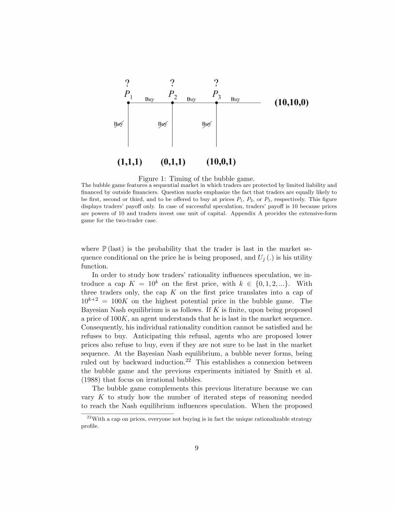
The timing of the bubble game is depicted in Figure 1.21 Speculating isprofitable for trader j if the following individual rationality (IRj) conditionis satisfied:

[1− P (last)]× P (next trader buys)× Uj (10)

+{[1− P (last)]× P (next trader doesn’t buy) + P (last)}×Uj (0) ≥ Uj (1) ,

19This experimental procedure corresponds to the strategy method. When a trader doesnot accept to buy the asset, subsequent traders end up with their initial wealth whatevertheir decision. The advantage of this method is that we can observe traders’ speculationdecision even if a bubble does not actually develop.

20When traders are self-financed, payoffs’ absolute values are scaled up by Pt. Intro-ducing traders’ limited liability and outside financiers undoes this scaling. This changehas some relevance from a practical point of view because most traders do have limitedliability and invest other people’s money. This change can also have some consequencesfor behavior in our experiment (as well as in practice): the stakes being smaller than whenthey are self-financed, traders might have more incentive to enter into bubbles.

21This timing does not correspond to the extensive form of the game. Indeed, it leavesaside the issue of which player is first, second, or third. The extensive-form game isprovided in Appendix A for the two-trader case. When there is no cap on the first price,it includes an infinite number of nodes.

8

? ? ?

Figure 1: Timing of the bubble game.The bubble game features a sequential market in which traders are protected by limited liability andfinanced by outside financiers. Question marks emphasize the fact that traders are equally likely tobe first, second or third, and to be offered to buy at prices P1, P2, or P3, respectively. This figuredisplays traders’ payoff only. In case of successful speculation, traders’ payoff is 10 because pricesare powers of 10 and traders invest one unit of capital. Appendix A provides the extensive-formgame for the two-trader case.

where P (last) is the probability that the trader is last in the market se-quence conditional on the price he is being proposed, and Uj (.) is his utilityfunction.

In order to study how traders’ rationality influences speculation, we in-troduce a cap K = 10k on the first price, with k ∈ {0, 1, 2, ...}. Withthree traders only, the cap K on the first price translates into a cap of10k+2 = 100K on the highest potential price in the bubble game. TheBayesian Nash equilibrium is as follows. If K is finite, upon being proposeda price of 100K, an agent understands that he is last in the market sequence.Consequently, his individual rationality condition cannot be satisfied and herefuses to buy. Anticipating this refusal, agents who are proposed lowerprices also refuse to buy, even if they are not sure to be last in the marketsequence. At the Bayesian Nash equilibrium, a bubble never forms, beingruled out by backward induction.22 This establishes a connexion betweenthe bubble game and the previous experiments initiated by Smith et al.(1988) that focus on irrational bubbles.

The bubble game complements this previous literature because we canvary K to study how the number of iterated steps of reasoning neededto reach the Nash equilibrium influences speculation. When the proposed

22With a cap on prices, everyone not buying is in fact the unique rationalizable strategyprofile.

9

price is P = 100K, an agent knows that he is last and no iterated step ofreasoning is needed. When the proposed price is P = 10K, a subject knowsthat he is not first in the market sequence (he can be second or third). Atequilibrium, he has to anticipate that the next trader in the market sequence(if any) would not accept to buy the asset. One step of iterated reasoningis thus needed to derive the equilibrium strategy. More generally, when theproposed price is 1 ≤ P ≤ 100K, the required number of iterated steps ofreasoning is log10

(100KP

). In order to study whether this required number

of iterated steps of reasoning affects bubble formation, we have chosen toexperimentally study treatments in which K equals 1, 100, and 10,000.

Another interesting aspect of our design is that we can let K go to in-finity. A bubble can arise at equilibrium if the (IRj) condition is satisfiedfor all traders on the market. It is straightforward to show that, if tradersanticipate that other traders speculate, there indeed exists increasing andconcave utility functions Uj (.) for which this (IRj) condition holds. Thebubble game thus offers an economic environment in which rational bub-bles can form despite the number of trades being finite and the existenceof the bubble being common knowledge. Hence our paper contributes tothe literature on rational bubbles by showing that neither infinite tradinghorizon (see Blanchard (1979) and Tirole (1982)) nor infinite trading speed(see Allen and Gorton (1993) and Abreu and Brunnermeier (2003)) are nec-essary for common knowledge rational bubbles to exist.23 The possibility ofequilibrium bubbles in our setting arises because no trader is ever sure tobe last in the market sequence.24

In order to show that the bubble equilibrium is meaningful, we now checkwhether financiers are willing to fuel the bubble. It is clear that, if the samefinancier provides capital to all traders (as it is the case in the experiment),his total expected profit would be negative. However, we show below that,if each trader has a different outside financier, these financiers may havean interest in providing capital to traders. Assuming that a financier has autility function denoted by Uf (.) and an initial wealth denoted by W , hisindividual rationality condition (IRf) is written as:

23In the previous models, two dimensions of infinity were required for bubbles to emergeat equilibrium: infinite trading opportunities and potentially infinite prices. We show thatonly this last dimension of infinity is necessary for common knowledge rational bubblesto arise at equilibrium.

24It is straightforward to show that a no-bubble equilibrium always exists. The Supple-mentary Appendix proves the existence of a bubble equilibrium for the risk neutral andconstant relative risk aversion cases. It also offers a more extensive theoretical analysis ofthe bubble game including a welfare analysis.

10

[1− P (last)]P (next trader buys)Uf (W + 10Pt − 10)

+ {[1− P (last)]× P (next trader doesn’t buy) + P (last)}× Uf (W − Pt + 1) ≥ Uf (W ) ,

for all Pt. It is again straightforward to show that, if financiers expectthat all traders speculate, there exist functions Uf (.) for which the (IRf)condition holds.

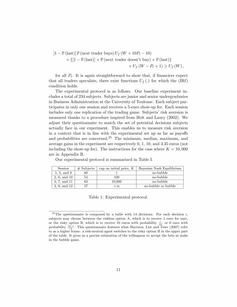
The experimental protocol is as follows. Our baseline experiment in-cludes a total of 234 subjects. Subjects are junior and senior undergraduatesin Business Administration at the University of Toulouse. Each subject par-ticipates in only one session and receives a 5-euro show-up fee. Each sessionincludes only one replication of the trading game. Subjects’ risk aversion ismeasured thanks to a procedure inspired from Holt and Laury (2002). Weadjust their questionnaire to match the set of potential decisions subjectsactually face in our experiment. This enables us to measure risk aversionin a context that is in line with the experimental set up as far as payoffsand probabilities are concerned.25 The minimum, median, maximum, andaverage gains in the experiment are respectively 0, 1, 10, and 3.35 euros (notincluding the show-up fee). The instructions for the case where K = 10, 000are in Appendix B.

Our experimental protocol is summarized in Table I.

Session # Subjects cap on initial price, K Bayesian Nash Equilibrium

1, 5, and 9 60 1 no-bubble

2, 6, and 10 54 100 no-bubble

3, 7, and 11 63 10,000 no-bubble

4, 8, and 12 57 +∞ no-bubble or bubble

Table 1: Experimental protocol.

25The questionnaire is composed by a table with 14 decisions. For each decision i,subjects may choose between the riskless option A, which is to receive 1 euro for sure,or the risky option B, which is to receive 10 euros with probability i

14, or 0 euro with

probability 14−i14

. This questionnaire features what Harrison, List and Towe (2007) referto as a higher frame: a risk-neutral agent switches to the risky option B in the upper partof the table. It gives us a precise estimation of the willingness to accept the bets at stakein the bubble game.

11

4 Behavioral game theory predictions

This section analyzes the game with various behavioral game theory mod-els. The next section structurally estimates these models using data fromthe bubble game. Two types of models appear relevant in our context: theSubjective Quantal Response Equilibrium (hereafter SQRE) of Rogers, Pal-frey, and Camerer (2009), and the Analogy-Based Expectation Equilibrium(hereafter ABEE) of Jehiel (2005). On the one hand, the SQRE is of interesthere since i) it is based on the concept of noisy best-response that proved use-ful to explain failures of backward induction in previous experiments (seeCamerer (2003)), and ii) it allows for heterogeneity in agents’ rationalitythat could be an important driver of bubble formation. On the other hand,the ABEE is relevant here because i) belief formation about the likelihoodof speculation at each price being complicated, players might simplify theproblem as considered in this equilibrium concept, and ii) candidates foranalogy classes arise naturally in the bubble game.

4.1 Subjective Quantal Response Equilibrium

According to the SQRE logic, an agent’s payoff responsiveness, denoted byλi,s, depends on his type i and on his level of sophistication, denoted by s.SQRE then involves a stochastic choice model whereby the agent’s propen-sity to choose an action has a logistic form that depends on the expectedpayoff of this action given his information, and on his payoff responsiveness.The expected payoff from buying the asset conditional on being proposeda price P is denoted by ui,s(B|P ). The expected payoff from not buyingthe asset is denoted by u∅. We adopt a specification with logistic stochasticchoice functions so that the probability that agent i buys the asset after

being proposed a price P is: Pi,s(B|P ) = eλi,sui,s(B|P )

eλi,sui,s(B|P )+eλi,su∅.

In the SQRE logic, agent i’s payoff responsiveness is given by: λi,s =λi + γs, where it is commonly known that λi is uniformly distributed overthe interval [Λ − ε

2 ,Λ + ε2 ], and where γ represents the sensitivity of an

agent’s payoff responsiveness to his level of sophistication. The level ofsophistication s follows a Poisson distribution with density function f . Letτ denote the average level of sophistication.

Finally, in the SQRE logic, agents may not have the same understandingof the overall population of players. In particular, it is assumed that anagent with sophistication s cannot imagine that other agents can have asophistication greater than s − θ. The agent’s truncated beliefs about the

12

fraction of h-level players is thus gs(h) = f(h)∑max(s−θ,0)i=0 f(i)

. The expected payoff

from buying the asset conditional on being proposed a price P can thus be

written as: ui,s(B|P ) = 10 [1− P(last|P )]∑max(s−θ,0)

h=0 gs(h)Pi′,h(B|10P ).26

Overall, SQRE has five parameters: Λ, the basic payoff responsiveness; ε,the uncertainty surrounding the basic payoff responsiveness; τ , the averagelevel of sophistication; γ, the sensitivity of payoff responsiveness to sophis-tication; and θ, the imagination parameter. As noted by Rogers, Palfrey,and Camerer (2009), SQRE is useful to incorporate the notion of skill. Skillis captured by the payoff responsiveness parameter λi,s. The higher thisparameter is, the more responsive the player is to payoffs and the betterhe perceives other players’ skills. This player might misperceive the distri-bution of skill in the population but, conditional on a skill level, he holdscorrect beliefs on the choice probabilities.

One advantage of using the SQRE is that it nests various interestingbehavioral game theory models. In particular, when Λ = 0, ε = 0, γ = +∞and θ = 1, the SQRE boils down to the Cognitive Hierarchy model (here-after CH) developed by Camerer, Ho and Chong (2004) with only one freeparameter τ . The CH model states that agents best-respond to mutuallyinconsistent beliefs: they believe that all other agents’ sophistication is lowerthan theirs.27 Moreover, agents with a level of sophistication s = 0 chooseeach available action with an equal probability. Alternatively, when ε = 0,θ = +∞, and when γ = 0 or τ = 0, the SQRE corresponds to the Quan-tal Response Equilibrium (hereafter QRE) of Mc Kelvey and Palfrey (1995)with only one free parameter Λ. The QRE takes into account the fact thatplayers make mistakes but it retains beliefs’ consistency. At equilibrium,players are responsive to payoffs to the extent that more profitable actions

26Given our experimental design, subjects play a simultaneous-move game in which de-cisions matter only if previous traders in the market sequence, if any, decide to buy theasset. We calculate expected payoffs conditional on this event in order to simplify equi-librium computations. Our specification of the QRE thus corresponds to Mc Kelvey andPalfrey (1998)’s Agent QRE in which agents play only once. An alternative specificationis to compute expected payoffs ex-ante, that is, taking into account the probability thatprevious players, if any, decide to buy. We checked that, when estimated on the entiredata, the quantal response equilibrium has a better fit with our specification than withthe ex-ante specification (p-value is 0.00 with a Vuong test).

27The level-k model of Stahl and Wilson (1995) and Nagel (1995) also exhibits suchdownward looking beliefs. The difference between these models and the CH model is thatthey assume that agents believe that all other agents have a level of sophistication thatis just below theirs. See also Costa-Gomes, Crawford, and Broseta, (2001), Costa-Gomesand Crawford (2006), and Crawford and Iriberri (2007) for experimental studies of thelevel-k model.

13

are chosen more often. Using the SQRE enables us to study whether noisybest-responses with beliefs consistency or best-responses with beliefs incon-sistencies best explain speculation in the bubble game.

Another advantage of the SQRE is that the QRE and CH models can beextended to take into account heterogeneity across agents. The CH modelcan be extended to a (discretized) Truncated Quantal Response Equilib-rium (hereafter TQRE) by setting γ < +∞. As a result, we have a CHmodel in which agents, instead of best-responding, have a payoff respon-siveness that increases with their level of sophistication. Likewise, the QREcan be extended to a Heterogeneous Quantal Response Equilibrium (here-after HQRE) by setting ε > 0. We then have a QRE in which agents donot know for sure what the exact level of payoff responsiveness of anotheragent is.28 Both of these extensions can prove useful to understand whetherheterogeneity across agents plays a role in bubble formation.

A last advantage of the SQRE is that is can be used to estimate whetheroverconfidence matters for speculative bubbles. The limited imagination pa-rameter θ indeed represents the extent to which agents underestimate theaverage level of sophistication in the population of players, a phenomenonwe refer to overconfidence because it is similar in spirit to the better-thanaverage effect in the psychology literature. Starting from the CH modeland freeing the parameter θ, we can estimate the extent to which agentssuffer from limited imagination. We call this model the overconfidence CH(hereafter OCH). θ positive corresponds to a high level of overconfidencebecause agents believe that all other players are less sophisticated than theyare. When θ is negative, agents conceive that other players may be more so-phisticated than them but they are still underestimating the average level ofsophistication due to their truncated beliefs. In the limit, when θ convergesto −∞, there is no overconfidence.

We now apply the SQRE to the bubble game. For brevity, we focus hereon the QRE and CH models for treatments with a finite price cap K.29

We first study the QRE. After being proposed a price P = 100K, atrader perfectly infers that he is last in the market sequence and buys with

28Uncertainty about other traders’ payoff responsiveness can be interpreted as uncer-tainty about their level of risk aversion.

29The computations for the general specification of the SQRE as well as for the casein which K = +∞ are available in the Supplementary Appendix. Extending the CH andQRE models to incorporate traders’ heterogeneity as modeled in the TQRE and HQREmodels does not change the underlying logic. For the case in which K = +∞, we derivepredictions by relying on equilibrium conjectures that are realized at equilibrium as it isthe case for the derivation of the Nash equilibrium.

14

probability P (B|P = 100K) = 11+eΛ

. After observing a price P = 10K, atrader infers that he has a specific probability, denoted by q(K,P = 10K),not to be last. He correctly anticipates that the probability to buy of the lasttrader is not equal to zero. His expected payoffs from buying is u(B|P =10K) = q(K,P = 10K) × 1

1+eΛ× 10. His probability to buy is therefore

P (B|P = 10K) = 1

1+eΛ×

(1− 10q(K,P=10K)

1+eΛ

) . Applying this logic backward, we

find the predicted probability that a trader buys at all potential prices. Thisanalysis shows that the QRE can predict the existence of bubbles even whenthere is a price cap.

Consider now the CH model. When proposed a price of 100K, a traderknows he is last in the sequence. Consequently, only level-0 traders buy,with probability 1

2 . Given that there is a fraction f (0) = τ0e−τ

0! of suchtraders in the population, the probability to observe a trader buying at thisprice is: P (B|P = 100K) = 1

2e−τ .

When a trader is being proposed a price P = 10K, he infers that he ispenultimate in the sequence. If he is a level-0 trader, he buys with prob-ability Ps=0(B|P = 10K) = 1

2 . If he is a level-s player with s ≥ 1, hethinks that the next trader observing the price 100K is a level-h with prob-ability gs(h) = f(h)∑s−1

i=0 f(i). Consequently, his expected profit if he buys is:

us≥1(B|P = 10K) = q(K,P = 10K) × f(0)∑s−1i=0 f(i)

× 12 × 10. The trader is

strictly better off buying if and only if∑s−1

i=0τ i

i! < 5q(K,P = 10K). Given

that∑s−1

i=0τ i

i! is strictly increasing in s, there exists a (potentially infinite)threshold s∗ ≥ 1 such that only traders with a level below or equal to s∗

buy. This is because higher level traders have a more accurate perception ofthe distribution of lower-level types. Finally, given the actual distributionof traders’ types, the probability to observe a trader buying at a price ofP = 10K is: P (B|P = 10K) = 1

2e−τ +

∑s=s∗

s=1

(τs

s! e−τ). As before, the rest of

the model is solved backward. The CH model can thus predict the existenceof bubbles despite the presence of a price cap.

4.2 Analogy-Based Expectation Equilibrium

According to the ABEE logic, agents use simplified representations of theirenvironment in order to form expectations. In particular, agents are assumedto bundle nodes of the game into analogy classes. 30 Agents then form

30Consistent with Jehiel (2005) when he studies endogenous analogy grouping (in page100), we consider that an agent’s bundling includes his own nodes. This specification ischosen for simplicity: it enables us to work with analogy classes that are constant across

15

correct beliefs concerning the average behavior within each analogy class.Following Huck, Jehiel, and Rutter (2011), we consider that agents applynoisy best-responses to their beliefs.31

In the bubble game, two types of analogy classes arise naturally. Onthe one hand, traders may use only one analogy class, assuming that othertraders’ behavior is the same across all potential prices. On the other hand,traders may use two analogy classes: one class (Class I) that includes pricesat which traders are sure not to be last in the market sequence, the other(Class II) that includes the remaining prices (at which traders think theymay be last or know they are last).

We now apply the ABEE to the bubble game. For brevity, we restrictour attention to the case in which the price cap is K = 1 (the other cases areaddressed in the Supplementary Appendix). Let p1, p2, and p3 denote theactual probability that a trader buys after observing prices equal to 1, 10,and 100, respectively. Let P(B|P = 1), P(B|P = 10), and P(B|P = 100) bethe corresponding probabilities as (mis)perceived by traders using analogyclasses.

We start by analyzing the one-class ABEE. A trader after observing aprice P = 100 knows he is last. Consequently, his probability to buy isp3 = 1

1+eΛ. A trader after observing a price P = 10 has the following

expected payoff from buying: u(B|P = 10) = 10× P(B|P = 100). Becauseof the use of one analogy class, we have P(B|P = 100) = p1+p2+p3

3 .32 Theprobability to buy after P = 10 is therefore: p2 = 1

1+eΛ(1− 10

3 (p1+p2+p3)). A

trader after observing a price P = 1 has an expected payoff of u(B|P =1) = 10 × P(B|P = 10) = 10p1+p2+p3

3 . The probability to buy is therefore:p1 = p2. This analysis leaves us with a system of equations that can besolved numerically to find p1, p2, and p3.

We now turn to the two-class ABEE. As before, a trader after observing aprice P = 100 buys with a probability p3 = 1

1+eΛ. A trader after observing

a price P = 10 has the following expected payoff from buying: u(B|P =10) = 10×P(B|P = 100). Because Class II is a singleton, we have P(B|P =

players.31The ABEE concept with stochastic choice remains different from the QRE given that,

in the ABEE logic, agents have inaccurate expectations regarding other players’ behavior.One can thus test whether this inaccuracy helps explaining the data.

32The probability 13

corresponds to the ex-ante probability of observing prices of 1, 10 or100. Given our experimental design in which all agents have to pick an action irrespectiveof whether previous players have decided to buy or not, using this ex-ante probability isin line with the spirit of ABEE. If we had chosen an experimental design corresponding tothe extensive representation of the game, we would have P(B|P = 100) = p1+p1p2+p1p2p3

1+p1+p1p2.

16

100) = p3. Thus, we have p2 = 11+eΛ(1−10p3) . A trader after observing a price

P = 1 uses Class I to form his expectations and thus has an expected payoffof u(B|P = 1) = 10 × P(B|P = 10) = 10p1+p2

2 . The probability to buy istherefore: p1 = 1

1+eΛ(1−5(p1+p2)) . The system of equations can again be solvednumerically.

Overall, one can show that the ABEE can predict the presence of abubble even when there is a price cap. The intuition is as follows. Atthe ABEE, traders expect that the probability to buy is constant acrossdifferent prices. This leads them to overestimate the likelihood that tradersbuy towards the end of the market sequence. A bubble can also arise atequilibrium in the ABEE logic even if agents best-respond to their beliefs,that is, even if Λ = +∞.33

4.3 Implications of the behavioral game theory models forspeculative bubbles

We use the derivations provided in the previous subsections in order tohighlight the implications for speculative bubbles of the various behavioralgame theory models we consider. For simplicity, we focus on the case inwhichK = 1 and on the decision to buy after observing P = 10 and P = 100,the last two consecutive prices.

The QRE predicts that the probability to buy is P (B|P = 10) =

[1 + e

Λ(

1− 10

1+eΛ

)]−1

after observing P = 10, and P (B|P = 100) =[1 + eΛ

]−1after observing

P = 100. The propensity to buy when P = 100 is pretty low becausetraders can only lose by doing so. It is higher when P = 10 because thereis a chance that the next trader will buy. This higher chance of resellinginduces a higher propensity to speculate.34 The snowball effect in the QREmodel is thus due to the fact that the initial noise due to stochastic choiceis amplified when stepping back away from the maximum price. The QREpredicts a snowball effect when K = +∞.

33For example, one can check that the following strategy profile is an ABEE with oneanalogy class: traders buy after observing prices of 1 and 10 and do not buy after observinga price of 100. With two analogy classes, the following profile is an ABEE: traders buyafter observing a price of 1 and do not buy after observing prices of 10 and 100.

34It is not always true that, in the QRE, P(B|P = 10i

)> P

(B|P = 10i+1

). Con-

sider, for example, the general case with a cap K in which the probability that traderi is not to be last after observing P = 10i is denoted by q(K,P = 10i). We have

P(B|P = 10i

)=[1 + eΛ(1−10q(K,P=10i)P(B|P=10i+1))

]−1

. If q(K,P = 10i) is low enough

compared to q(K,P = 10i+1), it is possible that P(B|P = 10i

)< P

(B|P = 10i+1

).

17

The CH model predicts that P (B|P = 10) = 12e

−τ +∑s=s∗

s=1

(τs

s! e−τ) and

that P (B|P = 100) = 12e

−τ . s∗ is the highest level of sophistication s such

that the inequality∑s−1

i=0τ i

i! < 5 is satisfied. This inequality indicates thatan agent with sophistication s is better off speculating. The propensityto speculate when P = 100 is pretty low because only step-0 players buywith probability 1

2 . It is higher when P = 10 because some agents withhigher levels of sophistication also decide to speculate. The snowball effectin the CH model is thus due to an increase in the willingness to speculateof more sophisticated agents. Contrary to the QRE, for K = +∞, theCH model does not predict a snowball effect. Indeed, all traders have thesame propensity to buy for all prices: traders with s > 0 always speculatewhile traders with s = 0 speculate with probability 1

2 . Our experiment thusconstitutes a stringent test for the CH model.

To analyze the implications of ABEE for the bubble game, we focuson the one-class ABEE. This model predicts that a trader speculates with

probability p2 =

[1 + e

Λ(

1− 103

[(1+eΛ)

−1+2p2

])]−1

after observing P = 10,

and p3 = 11+eΛ

after observing P = 100 (p1, the probability to buy afterobserving P = 1, is equal to p2). For example, for Λ = 1, numerical com-putations yield p1 = p2 = 0.999 and p3 = 0.269. Because of analogy-basedexpectations, the trader who observes P = 10 believes that the probabilitythat the next trader buys is p1+p2+p3

3 instead of p3. In the case we consider,such erroneous beliefs induces him to overestimate the probability that thenext trader buys which increases his propensity to speculate.35 This rein-forces the snowball effect above what would be predicted by the QRE, evenin the case in which K = +∞.

5 Empirical Results

5.1 The determinants of speculation in the bubble game

We study individual decisions to buy the overvalued asset. Figure 2 plots,for each treatment, the proportion of buy decisions for each price level. Thenumber of times a given price has been proposed is indicated at the bottomof the bar. Below the horizontal axis, we explicitly indicate, for each price,

35It is not always the case that, in ABEE, traders overestimate the likelihood thatthe next trader speculates. Consider, for example, the two-class ABEE with K = 100.The trader observing P = 10 anticipates that the next trader is in Class II and that hisprobability to buy is p3+p4+p5

3. If p3 > p4 and p3 > p5, then the actual probability that

the next trader buys p3 is higher than the expected probability p3+p4+p53

.

18

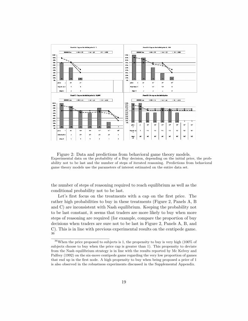
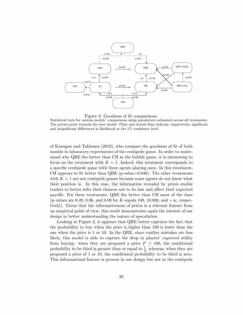
Figure 2: Data and predictions from behavioral game theory models.Experimental data on the probability of a Buy decision, depending on the initial price, the prob-ability not to be last and the number of steps of iterated reasoning. Predictions from behavioralgame theory models use the parameters of interest estimated on the entire data set.

the number of steps of reasoning required to reach equilibrium as well as theconditional probability not to be last.

Let’s first focus on the treatments with a cap on the first price. Therather high probabilities to buy in these treatments (Figure 2, Panels A, Band C) are inconsistent with Nash equilibrium. Keeping the probability notto be last constant, it seems that traders are more likely to buy when moresteps of reasoning are required (for example, compare the proportion of buydecisions when traders are sure not to be last in Figure 2, Panels A, B, andC). This is in line with previous experimental results on the centipede game.36

36When the price proposed to subjects is 1, the propensity to buy is very high (100% ofsubjects choose to buy when the price cap is greater than 1). This propensity to deviatefrom the Nash equilibrium strategy is in line with the results reported by Mc Kelvey andPalfrey (1992) on the six-move centipede game regarding the very low proportion of gamesthat end up in the first node. A high propensity to buy when being proposed a price of 1is also observed in the robustness experiments discussed in the Supplemental Appendix.

19

Also, keeping the number of steps of reasoning constant, it seems thattraders are more likely to buy when their probability not to be last increases(for example, compare the proportion of buy decisions for 3 and 4 stepsof reasoning in Figure 2, Panel B and C). This is a new empirical resultthat could not meaningfully be obtained in the centipede game because theprobability not to be last is equal to 1 for each node except the last one atwhich it is 0. This result indicates that there is some elements of rationalityin subjects’ decisions.

These results uncover a snowball effect: when there is a price cap, thepropensity to enter bubbles seems to increase with the required number ofreasoning steps and with the probability not to be last.

We now turn to the treatment in which there is no cap on the first price(Figure 2, Panel D), that is, K = +∞. First, subjects who are sure not tobe last always buy the asset which indicates a higher propensity to speculatethan when there is a price cap (for example, compare the proportion of buydecisions when traders are sure not to be last in Figure 2, Panels D, andC). A Wilcoxon rank sum test indicates that the proportion of buy decisionwhen subjects are offered a price of 1 or 10 is significantly higher whenK = +∞ (100%) than when there is one (77%) (the p-value is 0.034). 37

This is in line with the fact that bubbles are rational when K = +∞.Second, focusing exclusively on data from K = +∞, the probability to

buy appears to be statistically higher when subjects are sure not to be last(100%) than when they can be last (54%) (the p-value is 0.001 according toa Wilcoxon rank sum test). There is thus a snowball effect in the treatmentwith K = +∞. This is in contrast with the prediction of the CH model.

Third, when there is no cap and when prices are 100 or above, if partici-pants coordinate on the same equilibrium, their decisions should be the samefor all price levels. In line with this hypothesis, using a Wilcoxon rank sumtest, we cannot reject the fact that the probability to buy is the same afterobserving prices of 100, 1,000, and 10,000 (57%), and after observing higherprices (46%) with a p-value of 0.52 (this test keeps the required number ofsteps constant and equal to infinity).

These three results on the treatment with no cap cannot be obtained inan experiment with the centipede game, and underline the interest of ourdesign for the study of speculation.

In order to deepen our statistical analysis, we run a logit regression of

37This result however does not hold if we compare the cases K = +∞ (100%) andK = 10, 000 (92%) (the p-value is 0.261). Besides, there is no difference in the probabilityto buy when a subject has a probability not to be last equal to 3

7or 1

2between the cases

K = +∞ (54%) and K = 10, 000 (64%) (the p-value is 0.367).

20

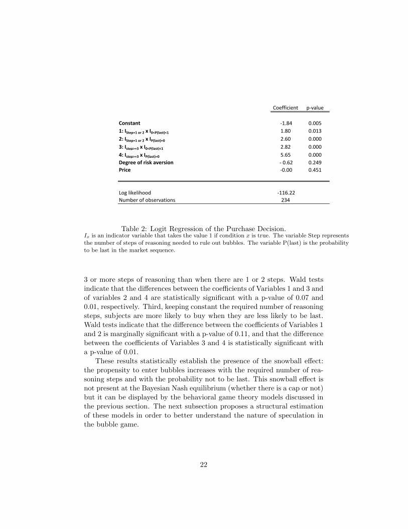
the propensity to buy the overvalued asset.38 As can be seen in Table II, thefirst four explanatory variables are constructed by interacting variables thatmeasure the number of steps of reasoning required to reach equilibrium andthe probability to be last. The last two variables are the individual degreeof risk aversion and the offered price.39 The constant reflects the propensityto speculate of subjects who are proposed to buy at the maximum price(100K), if any.40 This is useful because, since these subjects are expectednot to buy, their probability to buy can be viewed as the incompressiblelevel of noise in our data.

The results are in Table II. We first focus on the subjects who know theyare last in the market sequence. We can reject the hypothesis that thesesubjects never enter the bubble. Out of the 29 subjects who knew theywere last, three bought the asset.41 This number is low but it is not zero.This result is in line with the findings of Lei, Noussair and Plott (2001) thatsubjects were buying an overvalued asset even when prohibited to resell.In our framework, these agents correspond to “step 0” subjects. Lei etal. (2001) report in page 853 that 6 out of 36 subjects made at least onedominated transaction.42 This proportion (16.7%) is slightly higher thanour proportion of dominated choices (10.3%). We now complement theirresults by studying the behavior of subjects who are further away from themaximum price and who have more chances not to be last.

The regression analysis provides other interesting results. First, subjectswho have a chance not to be last buy significantly more than the ones whoknow they are last. Indeed, the coefficients of Variables 1 through 4 aresignificantly positive at the one percent level. Second, keeping constantthe probability to be last, subjects are more likely to buy when there are

38The results are the same if we run a probit regression.39The coefficient of risk aversion is computed assuming a constant relative risk aversion

utility function as in Holt and Laury (2002).40The regression also includes control variables that reflect the level of the cap in order

to test for treatment effects. These variables are omitted for the sake of brevity. None oftheir coefficient is statistically significant and the results do not change if we omit thesevariables from the analysis.

41None of the behavioral game theory models we consider can explain this phenomenonin a way more satisfying than stating that people make random errors. However, asexplained above, the various models have different implications regarding the impact ofthese errors on the market.

42We focus here on the experiment of Lei, Noussair and Plott (2001) during whichsubjects could participate in several markets, the so-called TwoMarket/NoSpec treatment.This is because, in this treatment, subjects could participate actively in the experimentwithout being forced to participate in the bubble. This provides a lower bound for thenumber of subjects who make mistakes in the market.

21

Coefficient p-value

Constant -1.84 0.005

1: IStep=1 or 2 x I0<P(last)<1 1.80 0.013

2: IStep=1 or 2 x IP(last)=0 2.60 0.000

3: Istep>=3 x I0<P(last)<1 2.82 0.000

4: Istep>=3 x IP(last)=0 5.65 0.000

Degree of risk aversion - 0.62 0.249

Price -0.00 0.451

Log likelihood -116.22

Number of observations 234

Table 2: Logit Regression of the Purchase Decision.Ix is an indicator variable that takes the value 1 if condition x is true. The variable Step representsthe number of steps of reasoning needed to rule out bubbles. The variable P(last) is the probabilityto be last in the market sequence.

3 or more steps of reasoning than when there are 1 or 2 steps. Wald testsindicate that the differences between the coefficients of Variables 1 and 3 andof variables 2 and 4 are statistically significant with a p-value of 0.07 and0.01, respectively. Third, keeping constant the required number of reasoningsteps, subjects are more likely to buy when they are less likely to be last.Wald tests indicate that the difference between the coefficients of Variables 1and 2 is marginally significant with a p-value of 0.11, and that the differencebetween the coefficients of Variables 3 and 4 is statistically significant witha p-value of 0.01.

These results statistically establish the presence of the snowball effect:the propensity to enter bubbles increases with the required number of rea-soning steps and with the probability not to be last. This snowball effect isnot present at the Bayesian Nash equilibrium (whether there is a cap or not)but it can be displayed by the behavioral game theory models discussed inthe previous section. The next subsection proposes a structural estimationof these models in order to better understand the nature of speculation inthe bubble game.

22

5.2 Estimating behavioral game theory models of specula-tion

Our results so far suggest that some players have bounded rationality andthat the formation of bubbles is related to a snowball effect. To account forthese phenomena, we estimate models that explicitly incorporate boundedrationality: the Subjective Quantal Response Equilibrium of Rogers, Palfrey,and Camerer (2009), and the Analogy-Based Expectation Equilibrium ofJehiel (2005).43 For each model, we estimate the parameters of interestusing maximum likelihood methods for the entire data set as well as foreach treatment separately.44 Confidence intervals are computed using abootstrapping procedure: using the empirical distribution of the observeddata, we resample 10,000 data sets on which the parameters of interest arere-estimated. We then choose the 2.5 and 97.5 percentile points values toconstruct 95% confidence intervals. When comparing the fits of two models,we use a likelihood ratio test when the models are nested, and Vuong (1989)’stest when they are not. 45

Table III reports our estimation results, and Figure 3 displays the sta-tistical tests for various models’ comparisons. The first two lines of TableIII describe our data, namely, the number of observations, and the observedaverage probability to buy. The next two lines show the predictions andlog-likelihoods of the Nash equilibrium under risk neutrality.46 The meanchoices are generally far away from the Nash equilibrium; the observed prob-ability to buy is too low when there exists a bubble-equilibrium, and toohigh when it does not exist.

Table III then provides the predictions and log-likelihoods of the various

43We initially planned to estimate the quantal response equilibrium and the cognitivehierarchy model. Following suggestions from the referees, we decided to estimate theSubjective Quantal Response Equilibrium which nests these two models, and the Analogy-Based Expectation Equilibrium.

44For simplicity, when estimating the Truncated Quantal Response Equilibrium andthe general Subjective Quantal Response Equilibrium models, we set θ = 1 as in the CHmodel.

45Under the null hypothesis, the probability distribution of the log-likelihood ratio statis-tic used to test nested models is approximated by a Chi-squared distribution with degreesof freedom equal to the difference between the numbers of parameters in the two models,while the probability distribution of the Vuong’s statistic used to test non-nested modelsis a standard normal distribution.

46We consider that traders coordinate on the bubble equilibrium when there is no capon the initial price. The no-bubble Nash equilibrium has a lower log-likelihood. In orderto compute the likelihoods, we assume that players choose non-equilibrium strategies witha probability of 0.0001.

23

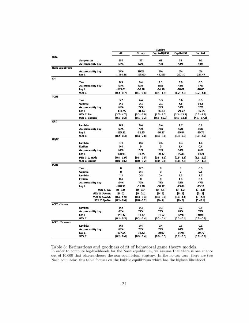
Table 3: Estimations and goodness of fit of behavioral game theory models.In order to compute log-likelihoods for the Nash equilibrium, we assume that there is one chanceout of 10,000 that players choose the non equilibrium strategy. In the no-cap case, there are twoNash equilibria: this table focuses on the bubble equilibrium which has the highest likelihood.

24

SQRE and ABEE models including the Cognitive Hierarchy model and itsextension, the Truncated Quantal Response Equilibrium, and the QuantalResponse equilibrium and its extension, the Heterogeneous QRE (hereafterHQRE), and the one- and two-classes ABEE. For brevity, the estimation ofthe Overconfidence Cognitive Hierarchy model is given in the SupplementaryAppendix.

The results are as follows. The average level of sophistication τ of theCH, estimated on the entire data set, is 0.5. This is in line with the medianestimates reported by Camerer, Ho and Chong (2004) that lie between 0.7and 1.9, but is a little low. This low estimated τ suggests a high proportionof level-0 players, around 60%. Interestingly, what drives this result is notreally the fact that traders enter too much into bubbles when they shouldnot. Indeed the fact that there is only around 10% of subjects who buywhen they know they are last in the market sequence suggests a proportion oflevel-0 players equal to 20%. What explains the high estimated proportion oflevel-0 players is rather the fact that subjects do not buy as much as expectedby the cognitive hierarchy model (with a higher average sophistication level)when there is no cap on the initial price or when the cap is large. This canbe seen on Figure 2 that plots the predictions of the CH model using thebest-fitting value of τ estimated on the entire data set. CH embeds thebetter than average effect to the extent that traders believe that no otheragent does as many steps of reasoning as them. Our estimations of OCH(reported in the Supplementary Appendix) show that, when the parameterθ can be identified, we cannot reject the hypothesis that θ = 1, its CHrestriction. Overconfidence is thus an important feature that enables theCH logic to fit our data pretty well.

The payoff responsiveness Λ of the QRE, estimated on the entire dataset, is 0.3. This is consistent with the results of Mc Kelvey and Palfrey(1995) who report estimates between 0.15 and 3.3. As was also the case forthe CH model, such a low value of the responsiveness parameter is requirednot so much to explain why subjects buy when they should not (that is,when the offered prices are close to the price cap, if any) but to explainwhy they do not buy that much when they should (that is, when the offeredprices are low).

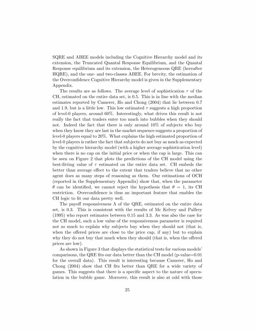
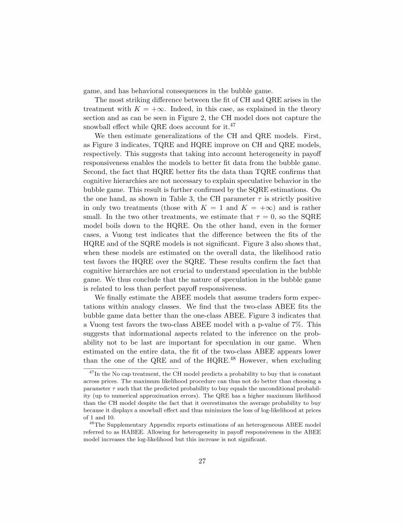
As shown in Figure 3 that displays the statistical tests for various models’comparisons, the QRE fits our data better than the CH model (p-value=0.01for the overall data). This result is interesting because Camerer, Ho andChong (2004) show that CH fits better than QRE for a wide variety ofgames. This suggests that there is a specific aspect to the nature of specu-lation in the bubble game. Moreover, this result is also at odd with those

25

p=0.00

p=0.00

p=0.03

p=0.00

Free

p=0.01

p=0.00

p=0.00 p=0.00

→∞ →∞

→∞

1

==0

=0

=0

→∞

HQRE TQRE

OCH

SQRE

CH QRE

Nash

ABEE 2 classes

p=0.02 p=0.07

p=0.01

p=0.00

p=0.12

ABEE 1 class

p=0.07

Figure 3: Goodness of fit comparisons.Statistical tests for various models’ comparisons using parameters estimated across all treatments.The arrows point towards the best model. Plain and dotted lines indicate, respectively, significantand insignificant differences in likelihood at the 1% confidence level.

of Kawagoe and Takizawa (2010), who compare the goodness of fit of bothmodels in laboratory experiments of the centipede game. In order to under-stand why QRE fits better than CH in the bubble game, it is interesting tofocus on the treatment with K = 1. Indeed, this treatment corresponds toa specific centipede game with three agents playing once. In this treatment,CH appears to fit better than QRE (p-value=0.046). The other treatmentswith K > 1 are not centipede games because some agents do not know whattheir position is. In this case, the information revealed by prices enabletraders to better infer their chances not to be last and affect their expectedpayoffs. For these treatments, QRE fits better than CH most of the time(p-values are 0.49, 0.06, and 0.00 for K equals 100, 10,000, and +∞, respec-tively). Given that the informativeness of prices is a relevant feature froman empirical point of view, this result demonstrates again the interest of ourdesign in better understanding the nature of speculation.

Looking at Figure 2, it appears that QRE better captures the fact thatthe probability to buy when the price is higher than 100 is lower than theone when the price is 1 or 10. In the QRE, since costlier mistakes are lesslikely, this model is able to capture the drop in players’ expected utilityfrom buying: when they are proposed a price P ≥ 100, the conditionalprobability to be third is greater than or equal to 1

2 , whereas, when they areproposed a price of 1 or 10, the conditional probability to be third is zero.This informational feature is present in our design but not in the centipede

26

game, and has behavioral consequences in the bubble game.The most striking difference between the fit of CH and QRE arises in the

treatment with K = +∞. Indeed, in this case, as explained in the theorysection and as can be seen in Figure 2, the CH model does not capture thesnowball effect while QRE does account for it.47

We then estimate generalizations of the CH and QRE models. First,as Figure 3 indicates, TQRE and HQRE improve on CH and QRE models,respectively. This suggests that taking into account heterogeneity in payoffresponsiveness enables the models to better fit data from the bubble game.Second, the fact that HQRE better fits the data than TQRE confirms thatcognitive hierarchies are not necessary to explain speculative behavior in thebubble game. This result is further confirmed by the SQRE estimations. Onthe one hand, as shown in Table 3, the CH parameter τ is strictly positivein only two treatments (those with K = 1 and K = +∞) and is rathersmall. In the two other treatments, we estimate that τ = 0, so the SQREmodel boils down to the HQRE. On the other hand, even in the formercases, a Vuong test indicates that the difference between the fits of theHQRE and of the SQRE models is not significant. Figure 3 also shows that,when these models are estimated on the overall data, the likelihood ratiotest favors the HQRE over the SQRE. These results confirm the fact thatcognitive hierarchies are not crucial to understand speculation in the bubblegame. We thus conclude that the nature of speculation in the bubble gameis related to less than perfect payoff responsiveness.

We finally estimate the ABEE models that assume traders form expec-tations within analogy classes. We find that the two-class ABEE fits thebubble game data better than the one-class ABEE. Figure 3 indicates thata Vuong test favors the two-class ABEE model with a p-value of 7%. Thissuggests that informational aspects related to the inference on the prob-ability not to be last are important for speculation in our game. Whenestimated on the entire data, the fit of the two-class ABEE appears lowerthan the one of the QRE and of the HQRE.48 However, when excluding

47In the No cap treatment, the CH model predicts a probability to buy that is constantacross prices. The maximum likelihood procedure can thus not do better than choosing aparameter τ such that the predicted probability to buy equals the unconditional probabil-ity (up to numerical approximation errors). The QRE has a higher maximum likelihoodthan the CH model despite the fact that it overestimates the average probability to buybecause it displays a snowball effect and thus minimizes the loss of log-likelihood at pricesof 1 and 10.

48The Supplementary Appendix reports estimations of an heterogeneous ABEE modelreferred to as HABEE. Allowing for heterogeneity in payoff responsiveness in the ABEEmodel increases the log-likelihood but this increase is not significant.

27

the treatment in which K = 1 that corresponds to a centipede game, thefit of the two-class ABEE is not significantly different at 5% than the oneof the QRE and of the HQRE. Furthermore, focusing on individual treat-ments, the fit of the two-class ABEE is never significantly different even at10% than the one of QRE. Compared to HQRE, it is significantly better at1% for K = +∞ and not significantly different at 5% for the other threetreatments. This suggests that analogy classes play an important role inunderstanding speculation as hypothesized by Bianchi and Jehiel (2011).

Moreover, the ABEE models appear better in terms of estimates’ sta-bility. Indeed, for the SQRE model and its various specifications, the pa-rameters of interest, estimated separately for each treatment, display somevariability: point estimates in Table III often vary by an order of magni-tude.49 For example, the estimates of Λ vary from 0.1 to 2.7 in the QREmodel and from 0.4 to 2.3 in the HQRE model. In contrast, the estimatesfrom the ABEE models appear quite stable across treatments.

6 Conclusion

This paper proposes a novel experimental design to study speculative be-havior in laboratory experiments: a bubble game in which agents tradesequentially and do not always know where they stand in the sequence. Ourgame has a no bubble Nash equilibrium when there is a finite price cap, andan additional bubble equilibrium when there is no price cap.

Analyzing our experimental data, some descriptive statistics show thatspeculation increases with the number of steps of iterated reasoning neededto reach equilibrium and with the probability that a subject is not last in themarket sequence. We then offer maximum likelihood estimations of variousbehavioral game theory models including, but not limited to, cognitive hi-erarchy (Camerer, Ho and Chong, 2004), quantal response equilibrium (McPalfrey and Palfrey, 1995), and analogy-based expectation equilibrium (Je-hiel, 2005). The main finding of the paper is that speculation in the bubblegame is related to quantal responses and analogy classes.

This finding echoes the results of Carrillo and Palfrey (2009, 2011) andCamerer, Nunnari, and Palfrey (2012) on other Bayesian games. Carrilloand Palfrey (2009) create and study the compromise game, and show that

49Such parameter estimates’ variability is not unusual in structural estimations of gametheory models. For example, in his Table 3, Weizsacker (2003) reports estimates of averagepayoff responsiveness that lie between 1.75 and 11.33 for player j. As indicated above,there is also some variability in the estimates of τ and Λ offered by Camerer, Ho, andChong (2004) and Mc Kelvey and Palfrey (1995), respectively.

28

a mix between the cursed equilibrium of Eyster and Rabin (2005) and thequantal response equilibrium best fits behavior in the compromise game.50

Carrillo and Palfrey (2011) and Camerer, Nunnari, and Palfrey (2012) fur-ther find that this cursed quantal response equilibrium also fits quite welldata from experiments with private information on bilateral trading gamesand auctions, respectively. Quantal responses and coarse thinking, an in-gredient of both the cursed equilibrium and the analogy-based expectationequilibrium, thus appears to be relevant to understand strategic behavior inBayesian games.

The experimental setting proposed in the present paper opens severalavenues of research. It would be interesting to study whether the occur-rence of bubbles (rational and irrational) vary with the number of traders,the introduction of risk in the underlying asset payoff, and the level of trans-parency (one could proxy for transparency by setting a non-null probabilitythat a trade is publicly announced). It would also be interesting to testwhether the structural estimations of behavioral game theory models wouldbe different after allowing for a high number of repetitions of the bubblegame. Finally, it could be fruitful to extend the experimental setting tocases in which the price path and the timing are left at the discretion oftraders. This would allow testing whether traders are able to coordinate ona price path and a timing that sustains rational bubbles.

50In a cursed equilibrium, agents underestimate the correlation between players’ infor-mation and action. As noted by Jehiel and Koessler (2008), the fully cursed equilibriumof Eyster and Rabin (2005) is equivalent to an ABEE in which analogy-classes correspondto the private information partition. Both equilibrium concepts incorporate a form ofcoarse thinking according to which agents reason in terms of categories. In the context ofABEE, agents reason in terms of categories of game nodes (the analogy classes) in whichthey expect behavior to be identical. In the context of cursed equilibrium, agents reasonin terms of categories of types that are assumed to have the same behavior.

29

7 Appendix

Appendix A: Extensive form of the game with two players

30

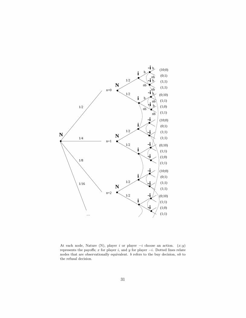
n=0

n=1

N N

N

i

i

i

-i

-i

-i

-i

-i

-i

-i

(10;0)

(0;1)

(1;1)

(1;1)

(0;10)

(1;1)

(1;0)

(1;1)

1/2

1/4

1/2

1/2

1/2

bb

nbb

nbb

nbb

nb

nb

b

nb

(10;0)

(0;1)

(1;1)

(1;1)n=1

n=2

N

i-i

-i

-i

-i

-i

-i

i

i

1/8

1/16

…

1/2

1/2

1/2

(0;10)

(1;1)

(1;0)

(1;1)

(10;0)

(0;1)

(1;1)

(1;1)

(0;10)

(1;1)

(1;0)

(1;1)

At each node, Nature (N), player i or player −i choose an action. (x; y)represents the payoffs; x for player i, and y for player −i. Dotted lines relatenodes that are observationally equivalent. b refers to the buy decision, nb tothe refusal decision.

31

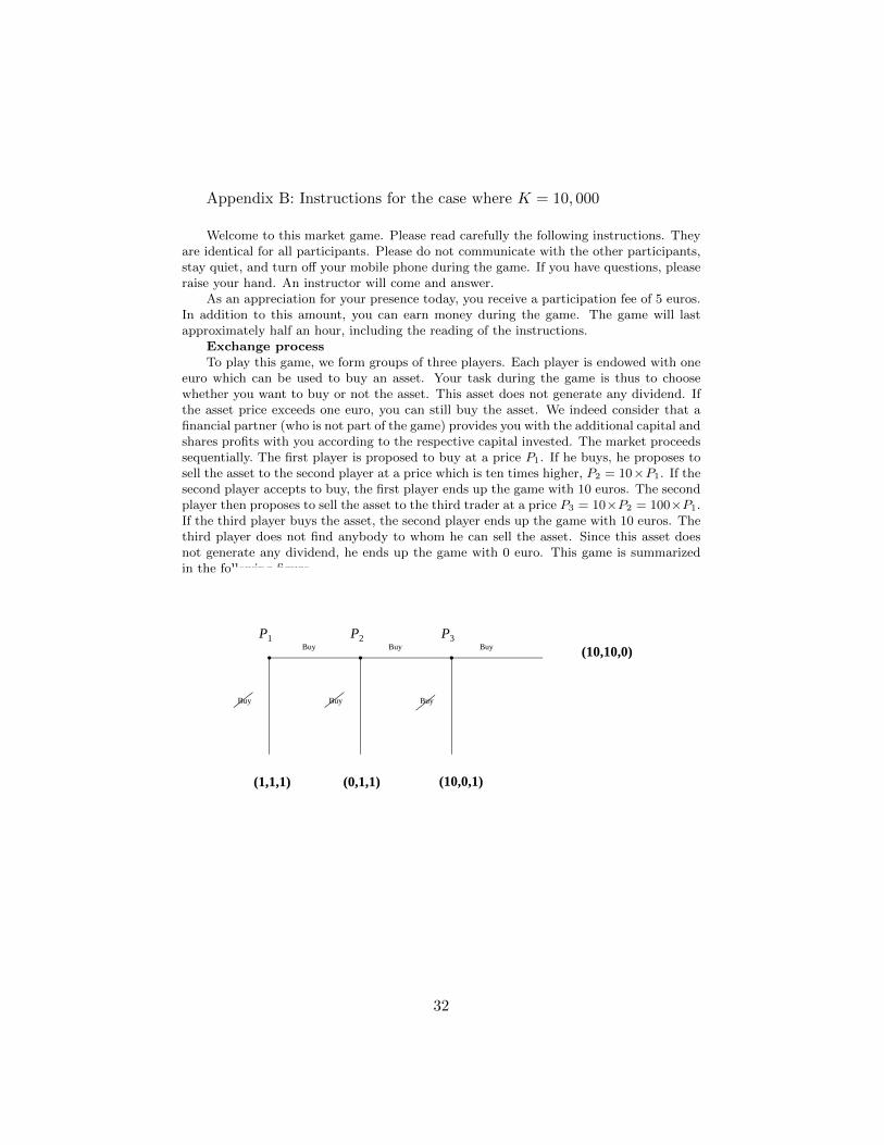
Appendix B: Instructions for the case where K = 10, 000

Welcome to this market game. Please read carefully the following instructions. Theyare identical for all participants. Please do not communicate with the other participants,stay quiet, and turn off your mobile phone during the game. If you have questions, pleaseraise your hand. An instructor will come and answer.

As an appreciation for your presence today, you receive a participation fee of 5 euros.In addition to this amount, you can earn money during the game. The game will lastapproximately half an hour, including the reading of the instructions.

Exchange processTo play this game, we form groups of three players. Each player is endowed with one

euro which can be used to buy an asset. Your task during the game is thus to choosewhether you want to buy or not the asset. This asset does not generate any dividend. Ifthe asset price exceeds one euro, you can still buy the asset. We indeed consider that afinancial partner (who is not part of the game) provides you with the additional capital andshares profits with you according to the respective capital invested. The market proceedssequentially. The first player is proposed to buy at a price P1. If he buys, he proposes tosell the asset to the second player at a price which is ten times higher, P2 = 10×P1. If thesecond player accepts to buy, the first player ends up the game with 10 euros. The secondplayer then proposes to sell the asset to the third trader at a price P3 = 10×P2 = 100×P1.If the third player buys the asset, the second player ends up the game with 10 euros. Thethird player does not find anybody to whom he can sell the asset. Since this asset doesnot generate any dividend, he ends up the game with 0 euro. This game is summarizedin the following figure.

Buy

Buy Buy

Buy Buy

Buy

P1 P2 P3

(10,10,0)

(1,1,1) (0,1,1) (10,0,1)

32

At the beginning of the game, players do not know their position in the marketsequence. Positions are randomly determined with one chance out of three for each playerto be first, second or third.

Proposed pricesThe price P1 that is proposed to the first player is random. This price is a power of

10 and is determined as follows:Price P1 Probability that this price is realized1 1/2 (50%)10 1/4 (25%)100 1/8 (12.5%)1,000 1/16 (6.3%)10,000 1/16 (6.3%)

Players decisions are made simultaneously and privately. For example, if the firstprice P1 = 1 has been drawn, the prices that are simultaneously proposed to the threeplayers are: P1 = 1 for the first player, P2 = 10 for the second player, and P3 = 100 forthe third player. Identically, if the first price P1 = 10, 000 has been drawn, the prices thatare simultaneously proposed to the three players are: P1 = 10, 000 for the first player,P2 = 100, 000 for the second player, and P3 = 1, 000, 000 for the third player.

The prices that you are been proposed can give you the following information regardingyour position in the market sequence:

- if you are proposed to buy at a price of 1, you are sure to be first;- if you are proposed to buy at a price of 10, you have one chance out of three to be

first and two chances out of three to be second in the market sequence;- if you are proposed to buy at a price of 100 or 1,000, you have one chance out of

seven to be first, two chances out of seven to be second, and four chances out seven to belast in the market sequence;

- if you are proposed to buy at a price of 10,000, you have one chance out of four tobe first, one chance out of four to be second, and two chances out four to be last.

- if you are proposed to buy at a price of 100,000, you have one chance out of two tobe second, and one chance out of two to be third.

- if you are proposed to buy at a price of 1,000,000, you are sure to be last.In order to preserve anonymity, a number will be assigned to each player. Once

decision will be made, we will tell you (anonymously) the group to which you belong, yourposition in the market sequence, if you are proposed to buy, and your final gain.

Do you have any question?

33

References

[1] Abreu D., and M. K. Brunnermeier, 2003, Bubbles and Crashes, Econometrica, 71(1),173-204.

[2] Ackert L. F., N. Charupat, B. K. Church, and R. Deaves, 2005, Bubbles in Experi-mental Asset Markets: Irrational Exuberance No More, mimeo.

[3] Ackert L. F., N. Charupat, R. Deaves, and B. Kluger, 2006, The Origins of Bubblesin Laboratory Asset Markets, mimeo.

[4] Allen, F., and G. Gorton, 1993, Churning Bubbles, Review of Economic Studies, 60,813-836.

[5] Allen, F., S. Morris, and A. Postlewaite, 1993, Finite Bubbles with Short-Sale Con-straints and Asymmetric Information, Journal of Economic Theory, 61, 206-229.

[6] Asparouhova, E., P. Bossaerts, and A. Tran, 2011, Market Bubbles and Crashes asan Expression of Tension between Social and Individual Rationality: Experiments,mimeo.

[7] Bianchi, M., and P. Jehiel, 2011, Bubbles and Crashes with Partially SophisticatedInvestors, mimeo.

[8] Blanchard O., 1979, Speculative Bubbles, Crashes, and Rational Expectations, Eco-nomic Letters, 3, 387-389.

[9] Brunnermeier M. K., 2009, Bubbles, Entry in The New Palgrave Dictionary of Eco-nomics, edited by Steven Durlauf and Lawrence Blume, 2nd edition.

[10] Brunnermeier M. K., and J. Morgan, 2010, Clock Games: Theory and Experiments,Games and Economic Behavior, 68, 532-550.

[11] Camerer C., 1989, Bubbles and Fads in Asset Prices: A Review of Theory andEvidence, Journal of Economic Surveys, 3, 3-41.

[12] Camerer C., 2003, Behavioral Game Theory: Experiments in Strategic Interaction,Princeton University Press.

[13] Camerer C., T.-H. Ho, and J.-K. Chong, 2004, A cognitive hierarchy model of one-shot games, Quarterly Journal of Economics, vol. 119, 861-898.

[14] Camerer C. and D. Lovallo, 1999, Overconfidence and Excess Entry: An Experimen-tal Approach, American Economic Review, 89, 306-318.

[15] Camerer C., S. Nunnari, and T. Palfrey, 2012, Quantal Response and NonequilibriumBeliefs Explain Overbidding in Maximum-Value Auctions, Caltech Social ScienceWorking Paper no. 1349.

[16] Carrillo J., and T. Palfrey, 2009, The Compromise Game: Two-Sided Adverse Selec-tion in the Laboratory, American Economic Journal: Microeconomics, 1, 151-181.

[17] Carrillo J., and T. Palfrey, 2011, No Trade, Games and Economic Behavior, 71,66-87.

[18] Conlon J., 2004, Simple Finite Horizon Bubbles Robust to Higher Order Knowledge,Econometrica, 72, 927-936.

[19] Cooper M.J., O. Dimitrov and R. Rau, 2001, A rose.com by Any Other Name, Journalof Finance, 56, 2371-2388.

34

[20] Costa-Gomes M., and V. Crawford, 2006, Cognition and Behavior in TwoPersonGuessing Games: An Experimental Study, American Economic Review, 96, 1737-1768.

[21] Costa-Gomes M., V. Crawford, and B. Broseta, 2001, Cognition and Behavior inNormal-Form Games: An Experimental Study, Econometrica, 69, 1193-1235.

[22] Crawford V., and N. Iriberri, 2007, Level-k Auctions: Can Boundedly RationalStrategic Thinking Explain the Winner’s Curse and Overbidding in Private-ValueAuctions?”, Econometrica, 75, 1721-1770.

[23] Doblas-Madrid A., 2012, A Robust Model of Bubbles with Multidimensional Uncer-tainty, Econometrica, 80, 1845-1893.

[24] Dufwenberg M., T. Lindqvist, and E. Moore, 2005, Bubbles and Experience: AnExperiment, American Economic Review, vol. 95, 1731-1737.

[25] Dulleck, U., and J. Oechssler, 1997, The absent-minded centipede, Economics Letters,vol. 55, 309-315.

[26] Eyster E. and M. Rabin, 2005, Cursed Equilibrium, Econometrica, 73, 1623-1672.

[27] Geanakoplos, J., 1992, Common Knowledge, Journal of Economic Perspectives, 6,52-83.

[28] Harrison G., J. List and C. Towe, 2007, Naturally Occurring Preferences and Exoge-nous Laboratory Experiments: A Case Study of Risk Aversion, Econometrica, 75,433-458.

[29] Holt, C. A., and S. K. Laury, 2002, Risk Aversion and Incentive Effects, AmericanEconomic Review, 92, 1644-1655.

[30] Huck, S., P. Jehiel, and T. Rutter, 2011, Feedback Spillover and Analogy-basedExpectations: a Multi-Game Experiment, Games and Economic Behavior, 71, 351-365.

[31] Jehiel, P., 2005, Analogy-based expectation equilibrium, Journal of Economic The-ory, 123, 81-104.

[32] Jehiel, P., and F. Koessler, 2008, Revisiting Games of Incomplete Information withAnalogy-Based Expectations, Games and Economic Behavior, 62, 533-557.

[33] Kawagoe, T. and H. Takizawa, 2010, Level-K Analysis of Experimental CentipedeGames, mimeo.

[34] Lei V., C. Noussair and C. Plott (2001), Nonspeculative Bubbles in ExperimentalAsset Markets: Lack of Common Knowledge of Rationality vs. Actual Irrationality,Econometrica, 69(4), 831.859.

[35] Mc Kelvey, R. D., and T. R. Palfrey, 1992, An Experimental Study of the CentipedeGame, Econometrica, vol. 60, 803-836.

[36] Mc Kelvey, R. D. and T. R. Palfrey, 1995, Quantal Response Equilibrium for NormalForm Games, Games and Economic Behavior, 10, 6-38.

[37] Mc Kelvey, R. D. and T. R. Palfrey, 1998, Quantal Response Equilibrium for Exten-sive Form Games, Experimental Economics, 1, 9-41.

[38] Moinas, S. and S. Pouget, 2012, Supplementary Appendix to “The Bubble Game:An Experimental Study of Speculation”, mimeo.

35

[39] Morris, S., A. Postlewaite, and H. Shin, 1995, Depth of Knowledge and the Effect ofHigher Order Uncertainty, Economic Theory, 6, 453-467.

[40] Morris, S., R. Rob, and H. Shin, 1995, p-Dominance and Belief Potential, Economet-rica, 63, 145-157.

[41] Nagel, R., 1995, Unraveling in Guessing Games: An Experimental Study, AmericanEconomic Review, 85, 1313-1326.

[42] Nalebuff, B., 1989, The Other Person’s Envelope is Always Greener, The Journal ofEconomic Perspectives, Vol. 3, 171-181.

[43] Noussair, C., S. Robin, and B. Ruffieux, 2001, Price Bubbles in Laboratory AssetMarkets with Constant Fundamental Values, Experimental Economics, 4, 87-105.

[44] Palfrey, T., and S. Wang, 2012, Speculative Overpricing in Asset Markets with In-formation Flows, Econometrica, 60, 1937-1976.

[45] Porter, D. P & Smith, V. L, 1995, Futures Contracting and Dividend Uncertainty inExperimental Asset, University of Chicago Press, vol. 68, 509-41.

[46] Rogers, B., T. Palfrey, and C. Camerer, 2009, Heterogeneous Quantal ResponseEquilibrium and Cognitive Hierarchies, Journal of Economic Theory, 144, 1440-1467.

[47] Smith V., G. Suchanek, and A. Williams, 1988, Bubbles, Crashes, and EndogenousExpectations in Experimental Spot Asset Markets, Econometrica, 56, 1119-1151.

[48] Stahl, D., and P. Wilson, 1995, On Players Models of Other Players: Theory andExperimental Evidence, Games and Economic Behavior, 10, 213-254.

[49] Tirole J., 1982, On the possibility of speculation under rational expectations, Econo-metrica, 50, 1163-1181.

[50] Tirole J., 1985, Asset Bubbles and Overlapping Generations, Econometrica, 53, 1499-1528.

[51] Van Boening, M.V., Williams, A.W., and LaMaster S. 1993. Price bubbles andcrashes in experimental call. markets. Economic Letters, 41, 179-185.

[52] Vuong, Q., 1989, Likelihood Ratio Tests for Model Selection and non-nested Hy-potheses, Econometrica, 57, 307-333.

[53] Weil P., 1987, Confidence and the Real Value of Money in an Overlapping GenerationsEconomy, Quarterly Journal of Economics, 102, 1-22.

[54] Weizsacker G., 2003, Ignoring the Rationality of Others: Evidence from ExperimentalNormal-form Games, Games and Economic Behavior, 44, 145-171.

[55] Xiong W. and J. Yu, 2011, The Chinese Warrants Bubble, American Economic Re-view, 101, 2723-2753.

36