The Birch and Swinnerton-Dyer conjecture for the Mazur
105
The Birch and Swinnerton-Dyer conjecture for the Mazur-Kitagawa p-adic L-function in the presence of an exceptional zero Gabriel Gauthier-Shalom Master of Science Department of Mathematics and Statistics McGill University Montreal,Quebec 2010-02-15 A thesis submitted to McGill University in partial fulfilment of the requirements of the degree of Master of Science. c Gabriel Gauthier-Shalom 2010
Transcript of The Birch and Swinnerton-Dyer conjecture for the Mazur
The Birch and Swinnerton-Dyer conjecture
for the Mazur-Kitagawa p-adic L-function
in the presence of an exceptional zero
Gabriel Gauthier-Shalom
Master of Science
Department of Mathematics and Statistics
McGill University
Montreal,Quebec
2010-02-15
A thesis submitted to McGill University in partial fulfilment of the requirements ofthe degree of Master of Science.
c© Gabriel Gauthier-Shalom 2010

ACKNOWLEDGEMENTS
I would like to thank my supervisor Henri Darmon for his infinite patience and
for his endlessly enthusiastic guidance. I would also like to thank Felicia Magpantay
for her moral support and technical help. I would lastly like to thank NSERC for
funding my graduate studies.
ii

ABSTRACT
Starting with the work of Mazur, Tate and Teitelbaum [17], various p-adic ana-
logues of the Birch and Swinnerton-Dyer conjecture have been formulated. The
case of an elliptic curve with split multiplicative reduction at the prime p is of spe-
cial interest. In this so called “exceptional zero” case, the order of vanishing of the
Mazur-Swinnerton-Dyer p-adic L-function at the central point seems to be one higher
than it is in the classical case. Greenberg and Stevens [10] proved results about this
conjecture, using properties of the two variable Mazur-Kitagawa p-adic L-function
Lp(E, k, s), which was defined in [14]. Their proof relies on the fact that the Mazur-
Kitagawa p-adic L-function Lp(E, k, s) vanishes along the central critical line s = k2,
and the fact that the restriction to k = 2 is equal to the Mazur-Swinnerton-Dyer
p-adic L-function attached to E. In the case where Lp(E, k,k2) is not identically
zero, a formula of Bertolini and Darmon [3] gives a formula for its second derivative
at k = 2. Their formula is also valid for twists Lp(E, χ, k, k2 ) of the L-function by
quadratic characters χ, and their method of proof relies essentially on the fact that χ
is quadratic. This thesis looks into possible generalizations of the result of Bertolini
and Darmon in the case of twists by Dirichlet characters of higher order.
iii

ABRÉGÉ
Depuis les travaux de Mazur, Tate et Teitelbaum [17], diverses conjectures ont
été proposées qui sont analogues à celle de Birch et Swinnerton-Dyer, dans le cas
p-adique. Cette thèse traite principalement le cas d’une courbe elliptique à réduction
multiplicative déployée en p; ce cas est dit “exceptionnel”. Dans ce cas, la multiplicité
de zéro de la fonction L de Mazur et Swinnerton-Dyer au point central semble être
une de plus que ce qui est prédit dans le cas classique. Greenberg et Stevens [10]
ont prouvé des résultats concernant cette conjecture en utilisant la fonction L de
Mazur et Kitagawa, qui est une fonction Lp(E, k, s) de deux variables. Leur preuve
se base sur le fait que la fonction L de Mazur et Kitagawa s’annule sur la ligne
centrale critique s = k2
et qu’elle est égal à la fonction L de Mazur et Swinnerton-
Dyer quand k = 2. Quand Lp(E, k,k2) ne s’annule pas, Bertolini et Darmon [3] ont
trouvé une formule pour la dérivée seconde de Lp(E, k, k2 ) en k = 2. Leur formule
tient encore quand on tord par un charactère quadratique. Cette thèse considère des
généralizations conjecturales des travaux de Bertolini et Darmon lorsque le caractère
est d’ordre supérieur à deux.
iv
TABLE OF CONTENTS
ACKNOWLEDGEMENTS . . . . . . . . . . . . . . . . . . . . . . . . . . . . ii
ABSTRACT . . . . . . . . . . . . . . . . . . . . . . . . . . . . . . . . . . . . iii
ABRÉGÉ . . . . . . . . . . . . . . . . . . . . . . . . . . . . . . . . . . . . . . iv
1 Introduction . . . . . . . . . . . . . . . . . . . . . . . . . . . . . . . . . . 1
1.1 Notation and conventions . . . . . . . . . . . . . . . . . . . . . . . 5
2 Modular forms . . . . . . . . . . . . . . . . . . . . . . . . . . . . . . . . 6
2.1 Definition . . . . . . . . . . . . . . . . . . . . . . . . . . . . . . . 62.2 Geometric interpretation . . . . . . . . . . . . . . . . . . . . . . . 9
2.2.1 Fundamental domains . . . . . . . . . . . . . . . . . . . . . 112.3 Congruence subgroups . . . . . . . . . . . . . . . . . . . . . . . . 122.4 The Hecke operators . . . . . . . . . . . . . . . . . . . . . . . . . 132.5 Homology . . . . . . . . . . . . . . . . . . . . . . . . . . . . . . . 15
2.5.1 Sign decomposition . . . . . . . . . . . . . . . . . . . . . . 202.6 Hecke module structure . . . . . . . . . . . . . . . . . . . . . . . . 20
2.6.1 Atkin-Lehner theory . . . . . . . . . . . . . . . . . . . . . . 222.6.2 The wQ operator . . . . . . . . . . . . . . . . . . . . . . . . 24
2.7 Calculating spaces of cusp forms . . . . . . . . . . . . . . . . . . . 252.8 Ordinary submodule . . . . . . . . . . . . . . . . . . . . . . . . . 25
3 L-functions and modular symbols . . . . . . . . . . . . . . . . . . . . . . 32
3.1 Modular symbols . . . . . . . . . . . . . . . . . . . . . . . . . . . 323.1.1 Modular symbols attached to a cusp form . . . . . . . . . . 333.1.2 Action of the Hecke operators . . . . . . . . . . . . . . . . 363.1.3 Sign decomposition . . . . . . . . . . . . . . . . . . . . . . 37
3.2 Explicit description . . . . . . . . . . . . . . . . . . . . . . . . . . 383.3 The L-function attached to a cusp form . . . . . . . . . . . . . . . 39
3.3.1 Twists . . . . . . . . . . . . . . . . . . . . . . . . . . . . . 41
v

3.4 The functional equation . . . . . . . . . . . . . . . . . . . . . . . 43
4 Elliptic Curves . . . . . . . . . . . . . . . . . . . . . . . . . . . . . . . . 46
4.1 Definition . . . . . . . . . . . . . . . . . . . . . . . . . . . . . . . 464.2 Group Structure . . . . . . . . . . . . . . . . . . . . . . . . . . . . 474.3 Reduction modulo primes . . . . . . . . . . . . . . . . . . . . . . 484.4 The L-function attached to an elliptic curve . . . . . . . . . . . . 504.5 The Modularity Theorem . . . . . . . . . . . . . . . . . . . . . . . 514.6 The Birch and Swinnerton-Dyer Conjecture . . . . . . . . . . . . . 524.7 The Twisted Birch and Swinnerton-Dyer Conjecture . . . . . . . . 54
5 The p-adic L-function . . . . . . . . . . . . . . . . . . . . . . . . . . . . 58
5.1 p-adic distributions . . . . . . . . . . . . . . . . . . . . . . . . . . 585.2 p-adic integrals . . . . . . . . . . . . . . . . . . . . . . . . . . . . 625.3 The p-adic L-function . . . . . . . . . . . . . . . . . . . . . . . . . 645.4 The p-adic L-series . . . . . . . . . . . . . . . . . . . . . . . . . . 655.5 Interpolation properties . . . . . . . . . . . . . . . . . . . . . . . . 675.6 Functional equation . . . . . . . . . . . . . . . . . . . . . . . . . . 685.7 The p-adic Birch and Swinnerton-Dyer conjectures . . . . . . . . . 695.8 Computational aspects . . . . . . . . . . . . . . . . . . . . . . . . 70
5.8.1 Calculating with overconvergent modular forms . . . . . . . 715.8.2 Solving the Manin relations . . . . . . . . . . . . . . . . . . 73
5.9 Computing the p-adic L-function . . . . . . . . . . . . . . . . . . 75
6 The Mazur-Kitagawa p-adic L-function . . . . . . . . . . . . . . . . . . . 77
6.1 Iwasawa algebras . . . . . . . . . . . . . . . . . . . . . . . . . . . 786.2 Hida family . . . . . . . . . . . . . . . . . . . . . . . . . . . . . . 826.3 Measure-valued modular symbols . . . . . . . . . . . . . . . . . . 84
6.3.1 Specialization maps . . . . . . . . . . . . . . . . . . . . . . 856.4 Defining properties . . . . . . . . . . . . . . . . . . . . . . . . . . 87
6.4.1 Ordinary part . . . . . . . . . . . . . . . . . . . . . . . . . 886.4.2 The symbol µ∗ . . . . . . . . . . . . . . . . . . . . . . . . . 90
6.5 The Mazur-Kitagawa p-adic L-function . . . . . . . . . . . . . . . 916.6 The exceptional zero conjecture . . . . . . . . . . . . . . . . . . . 926.7 The Birch and Swinnerton-Dyer conjecture in two variables . . . . 936.8 Continuing work . . . . . . . . . . . . . . . . . . . . . . . . . . . . 95
vi

References . . . . . . . . . . . . . . . . . . . . . . . . . . . . . . . . . . . . . . 96
vii

CHAPTER 1Introduction
The problem of finding rational solutions to polynomial equations has been a
focus of mathematics since ancient times. Many advances have been made, but some
of the most important questions remain unanswered. One important advance was
made by Hilbert and Hurwitz, who provided a general method of to find all rational
solutions to a quadratic equation in two variables (the genus 0 case). The problem of
finding rational points on curves of genus greater than 0 has proven to be much more
difficult. An important breakthrough was Faltings’ proof of Mordell’s conjecture,
which states that a curve of genus greater than one has only finitely many rational
points. Faltings’ result is unfortunately ineffective, so many questions still remain.
In contrast to Faltings’ theorem, curves of genus exactly 1 often contain infinitely
many rational points. Yet again there is no known method for determining whether
a genus 1 curve contains rational points. Much work has gone into classifying the
set of rational points on genus 1 curves that do contain rational points; a genus 1
curve with a fixed choice of a rational point is called an elliptic curve. An essential
tool in the study of an elliptic curve E is the fact that there exists a composition
law on the set E(Q) of rational points on E, which gives E(Q) a group structure.
A well known theorem of Mordell ensures that the group E(Q) is finitely generated,
though the set E(Q) itself is often infinite (as mentioned earlier). One of the most
interesting problems is that of finding the rank of E(Q), which is the Z-rank of
1

E(Q) modulo torsion. The problem of computing the rank of E(Q) would become a
simple computational problem if the Birch and Swinnerton-Dyer conjecture were to
be proven.
The Birch and Swinnerton-Dyer conjecture proposes that arithmetical infor-
mation about the rational points E(Q) of an elliptic curve E can be related to
the combined properties of E when reduced modulo each prime. The Hasse-Weil
L-function L(E, s) is the analytic object which encodes the combined information
about E modulo each prime. The function L(E, s) turns out to be a holomorphic
function on the whole complex plane, a fact which was established by the proof of
the modularity theorem; see §4.5 for an explanation. The Hasse-Weil L-function
satisfies a functional equation relating the values at s and 2 − s. Of interest is the
Taylor expansion of L(E, s) around the central point s = 1 of the symmetry of the
L-function. The Birch and Swinnerton-Dyer conjecture states that the order of van-
ishing of the Taylor expansion of L(E, s) around s = 1 is equal to the rank of E(Q).
Further, generalized versions of the Birch and Swinnerton-Dyer conjecture suggest
that more information about E can be gleaned from the leading coefficient of the
Taylor expansion. Specifically, it seems that the leading coefficient of the expansion
of L(E, s) around s = 1 is a product of various constants which encode arithmetical
information about E. More details on the Birch and Swinnerton-Dyer conjecture
can be found in Wiles’s millennium problem description [26].
A new direction of research arose with the introduction by Mazur and Swinnerton-
Dyer [16] of a p-adic analogue Lp(E, s) of the Hasse-Weil L-function. The Mazur-
Swinnerton-Dyer p-adic L-function Lp(E, s) attached to an elliptic curve E is a
2
p-adic analytic function which interpolates the so called “special values” of the Hasse-
Weil L-function. These “special values” are the values of twists of the Hasse-Weil
L-function at the central point 1. The development of the theory of p-adic L-functions
led Mazur, Tate and Teitelbaum [17] to formulate a p-adic analogue to the Birch and
Swinnerton-Dyer conjecture. The statement of the p-adic Birch and Swinnerton-Dyer
conjecture is largely similar to the classical case, with one important modification.
When E does not have split multiplicative reduction at the prime p, the statement
is analogous; the order of vanishing of the p-adic L-function at the central point is
conjectured to match the rank of E(Q). There is also a formula conjecturally relating
arithmetic information about E to the “leading coefficient” of the p-adic L-function.
In the remaining case, where E has split multiplicative reduction at p, the
statement of the p-adic Birch and Swinnerton-Dyer conjecture is slightly more com-
plicated. This complication is related to properties of the p-adic multiplier, which is
the factor that allows the special values of the classical L-function to be p-adically
interpolated. The p-adic multiplier vanishes exactly in the case of split multiplica-
tive reduction. The order of vanishing of the p-adic L-function then appears to be
thrown off, and is conjecturally one higher than the rank of E(Q). There is also an
additional factor that appears in the conjectural formula for the leading coefficient
of the p-adic L-series; this factor is referred to as the p-adic L -invariant for E and
is denoted Lp(E).
The authors of [17] empirically conjectured a formula which, in the rank 0 case,
expresses Lp(E) in terms of quantities arising from p-adic analytic properties of E.
Greenberg and Stevens [10] proved this “exceptional zero conjecture”. An essential
3

ingredient in their proof was a two-variable p-adic L-function Lp(E, k, s) called the
Mazur-Kitagawa p-adic L-function. For a fixed integer value k ≥ 2, the function
Lp(E, k, s) is a constant multiple of the one-variable Mazur-Swinnerton-Dyer p-adic
L-function of a modular form fk. The modular form f2 is in fact the weight 2 newform
attached to E via the modularity theorem, and the one-variable p-adic L-function
can be recovered from Lp(E, k, s) by fixing k = 2. Furthermore, the form fk is part
of the Hida family arising from f2. The Hida family is a collection of modular forms
of varying p-adic weight whose coefficients vary continuously with the weight.
The Mazur-Kitagawa p-adic L-function Lp(E, k, s) has a functional equation
relating its value at (k, s) to that at (k, k − s). Thus it is of interest to look at
the values of the Mazur-Kitagawa p-adic L-function along the critical line s = k2.
Bertolini and Darmon [3] proved the following theorem:
Theorem 1.1. Suppose that E has at least two primes of semistable reduction. Then
there is a global point P ∈ E(Q)⊗Q and a scalar ℓ ∈ Q× such that
d2
dk2Lp(k, k/2)k=2 = ℓ · logE(P )2
and the point P is of infinite order iff L′(E, 1) 6= 0.
Here logE is the formal group logarithm defined on E, and L(E, s) is the Hasse-
Weil L-function attached to E. In fact, the authors of [3] prove a more general
statement involving quadratic twists of the Mazur-Kitagawa p-adic L-function as
well. The purpose of this thesis is to look into possible generalizations of the results
of Bertolini and Darmon to characters of higher order.
4
1.1 Notation and conventions
The operation given by
a b
c d
7→
d −b
−c a
is called adjugation and will be denoted A 7→ A; it is an anti-involution on M2×2(R)
for any ring R (i.e. AB = BA) and preserves the determinant. Note that this
conveniently preserves integrality, and coincides with inversion on SL2(Z). Note also
that A = det(A)A−1. This is a useful operation for turning left actions into right
ones (or vice versa).
The completion of the algebraic closure of Qp will be denoted Cp. The algebraic
numbers Q will be viewed as being contained in Cp, via a fixed choice of embedding.
5

CHAPTER 2Modular forms
Modular forms are functions on the upper half-plane that satisfy many sym-
metries. They arise naturally in connection to problems related to quadratic forms,
and many other areas of mathematics. For example, the theory of modular forms
provides an easy proof to Lagrange’s four square theorem. This example and many
others are contained in the paper “Elliptic Modular Forms and Their Applications”
by Don Zagier [28]. The usefulness of modular forms derives in large part from the
finite dimensionality of spaces of modular forms for finite index subgroups of SL2(Z).
Modular forms are also very useful because of a connection to elliptic curves.
In fact, the coefficients of the L-function attached to a rational elliptic curve always
arise from the coefficients of a modular form. This was conjectured by Shimura and
Taniyama in the 1950s and proven in the early 2000s. The proof of this so called
“modularity theorem” is one of the most important number theoretic results in the
past century; see §4.5 for a description.
2.1 Definition
Let H = z ∈ C|ℜ(z) > 0 denote the upper half-plane. The group
GL2(Q) =
a b
c d
∣
∣
∣
∣
∣
∣
∣
a, b, c, d ∈ Q, ad− bc 6= 0
6
acts on H via
a b
c d
z =
az + b
cz + d. (2.1)
A straightforward calculation gives the formula
ℑ
a b
c d
z
=
ℑ(z)|cz + d|2 ,
which ensures that the action does indeed preserve the sign of the imaginary part
(and so is a well-defined action on H). Equation (2.1) is used to define a right action
of GL2(Q) on the set of functions from H to C; for an integer k, the weight k action
of GL2(Q) is defined, for
f : H → C and γ =
a b
c d
∈ GL2(Q)
by
(f |kγ)(z) = (det γ)k−1j(γ, z)−kf(γz),
with j(γ, z) := cz+d. Note that the scalar matrix λI acts as multiplication by λk−2.
The modular group is
SL2(Z) =
a b
c d
∣
∣
∣
∣
∣
∣
∣
a, b, c, d ∈ Z, ad− bc = 1
.
This group is generated by the matrices
S =
0 1
−1 0
and T =
1 1
0 1
.
7
The height of a subgroup Γ of the modular group SL2(Z) is the minimal h > 0 such
that the T h ∈ Γ, or infinity if Γ contains no power of T . For the rest of this chapter,
Γ ⊆ SL2(Z) will denote a finite index subgroup of SL2(Z). This implies that AΓA−1
is of finite height for all A ∈ SL2(Z).
A meromorphic function f on H satisfying f |kγ = f for all γ ∈ Γ is called weakly
modular of weight k with respect to Γ. Note then that for A ∈ SL2(Z), the function
f |kA is weakly modular with respect to A−1ΓA by a simple calculation. A weakly
modular function f for Γ on the upper half-plane satisfies f |kT h = f where h is the
height of Γ. Thus f(z + h) = f(z), so, assuming f is holomorphic on z | ℑ(z) > c
for some c > 0, we have that f has a Fourier expansion on that set:
f(z) =
∞∑
n=−∞anq
n
with q := e2πiz/h. The notation an(f) will be used to denote the coefficient of qn
in the Fourier expansion of such an f . The function f is said to be meromorphic
at ∞ if there is some m ∈ Z such that an(f) = 0 for all n < m. It is said to be
holomorphic at ∞ if an(f) = 0 for all n < 0. It is said to vanish at ∞ if, in addition
to being holomorphic, a0(f) = 0.
A meromorphic function f : H → C is called an automorphic form of weight k
with respect to a subgroup Γ of SL2(Z) if
• f |kγ = f ∀γ ∈ Γ,
• f |kA is meromorphic at ∞ for all A ∈ SL2(Z).
An automorphic form f is called a modular form of weight k with respect to Γ if it
satisfies the following additional property:
8
• f |kA is holomorphic at ∞ for all A ∈ SL2(Z).
Finally, a modular form f is called a cusp form if it satisfies the following additional
property:
• f |kA vanishes at ∞ for all A ∈ SL2(Z).
The space of automorphic forms of weight k for Γ will be denoted Ak(Γ); the cor-
responding spaces of modular and cusp forms will be respectively denoted Mk(Γ)
and Sk(Γ). Note the inclusions Ak(Γ) ⊃ Mk(Γ) ⊃ Sk(Γ). A cusp form f is called
normalized if a1(f) = 1. When working with forms of a fixed weight k, the weight k
action of GL2(Q) will sometimes be denoted without the subscript (i.e. the notation
f |γ will denote f |kγ when the weight is understood.)
2.2 Geometric interpretation
Automorphic forms can be interpreted geometrically. To do so, we must intro-
duce two varieties attached to a modular subgroup. The first is the open modular
curve attached to Γ, denoted Y (Γ). The set of complex points Y (Γ)(C) of Y (Γ) is
simply H modulo the action of Γ. A complex differentiable structure is defined on
Y (Γ)(C); details of this can be found, for example, in §2 of Diamond and Shurman’s
book [7].
To describe the next variety, we need to introduce the following topological set
first:
H∗ := H ∪ P1(Q) ⊂ P1(C)
The points corresponding to P1(Q) are called cusps. The action of SL2(Z) on H
extends to an action on H∗ in the obvious way. The topology of H is extended to
H∗ by defining the following local bases around the cusps:
9

• for the cusp ∞: sets of the form z ∈ H |ℑ(z) > N ∪ ∞.
• for a finite cusp r: the set of circles in H tangent to the real line at r.
The action of a matrix in SL2(Z) is seen to be continuous, since it takes members
of this basis to other members of this basis. The closed modular curve attached to
Γ is denoted X(Γ); it has complex points X(Γ)(C) corresponding to the quotient
of H∗ by the action of Γ. There is an embedding Y (Γ)(C) → X(Γ)(C), and the
complement of the image of Y (Γ)(C) is a finite set of points. These points are called
the cusps of X(Γ); they correspond to Γ-inequivalent cusps in P1(Q) ⊆ H∗. Details
of the construction of X(Γ)(C), and of the complex differentiable structure can be
found again in §2 of [7].
Now note the following calculation:
d(Az) = d
(
az + b
cz + d
)
=ad− bc
(cz + d)2dz
= det(A)(cz + d)−2dz = det(A)j(A, z)−2dz, (2.2)
which implies, for a form of weight 2k and γ ∈ Γ, that
f(γz)d(γz)k = j(γ, z)2kf(z)(j(γ, z)−2dz)k
= f(z)dzk.
Thus, f(z)dzk is invariant under the action of Γ, so should “descend” to a k-differential
on Y (Γ). This idea is made precise with the introduction of the space Ω(X(Γ))⊗k of
meromorphic k-differentials on X(Γ), whose details can be found in §3.3 of [7]. The
following is theorem 3.3.1 of [7]:
10

Theorem 2.1. The assignment f 7→ f(z)(dz)k is an isomorphism between A2k(Γ)
and Ω(X(Γ))⊗k for any positive integer k.
To be more explicit: if f ∈ A2k(Γ) corresponds to ω ∈ Ω(X(Γ))⊗k via this
isomorphism, then the pullback to H of ω is f(z)dzk. Theorem 2.1 tells us that
we can think of weight k automorphic forms for Γ as meromorphic k-differentials
on X(Γ). The subspaces of Ω(X(Γ))⊗k corresponding to the subspaces Mk(Γ) and
Sk(Γ) of Ak(Γ) can be described explicitly with inequalities on the order of vanishing
of the differentials at certain points. See §3.5 of [7] for more details.
2.2.1 Fundamental domains
A fundamental domain for the action of Γ ⊆ PSL2(Z) on H is a region F ⊂ H
with the following properties:
•⋃
γ∈ΓγF = H
• γInt(F) ∩ Int(F) = ∅ ∀γ ∈ Γ
• F is simply connected.
Here Int(F) denotes the interior of F . The points of a fundamental domain for
Γ are in one-to-one correspondence with the points of Y (Γ) via the quotient map.
Now define T to be the (hyperbolic) triangle passing through the cusps 0, 1 and
ρ := 1+√−3
2. Note that τ fixes ρ, and cycles 0, 1 and ∞. Define R := T ∪ τT ∪ τ 2T
to be the triangle passing through 0, 1 and ∞.
The region T is a fundamental domain for the group PSL2(Z). We can always
find a fundamental domain for Γ that consists of a union of translates of T by matrices
in G. If Γ has no torsion, then there is always a fundamental domain consisting of
translates of R. Fundamental domains are useful for explicitly describing spaces of
11
modular symbols, as will be explained in chapter 5, following Pollack and Stevens
[19].
2.3 Congruence subgroups
Now we will introduce the congruence subgroups of SL2(Z). The most important
congruence subgroups are:
Γ(N) :=
a b
c d
∈ SL2(Z)
∣
∣
∣
∣
∣
∣
∣
a b
c d
≡
1 0
0 1
mod N
,
Γ1(N) :=
a b
c d
∈ SL2(Z)
∣
∣
∣
∣
∣
∣
∣
a b
c d
≡
1 ∗
0 1
mod N
,
Γ0(N) :=
a b
c d
∈ SL2(Z)
∣
∣
∣
∣
∣
∣
∣
a b
c d
≡
∗ ∗
0 ∗
mod N
.
Note the inclusions Γ(N) ⊆ Γ1(N) ⊆ Γ0(N). More generally, a subgroup Γ ⊆ SL2(Q)
is called a congruence subgroup if ∃N with Γ(N) ⊆ Γ. In this case, the smallest
such N is called the level of Γ. Now we generalize the notion of modular form. A
Dirichlet character χ of period N can be viewed as a character on Γ0(N) by the rule
χ
a b
c d
= χ(d)
A simple calculation reveals that χ is indeed multiplicative for matrices in Γ1(N).
Definition 2.2. A modular form f for Γ1(N) is called a modular form for Γ0(N) of
weight k and character χ if it satisfies the additional property that f |γ = χ(γ)f for
all γ ∈ Γ0(N).
12

The space of all modular forms for Γ0(N) of weight k and character χ is denoted
Mk(N,χ). Note that if χ is the trivial character modulo N , then Mk(N,χ) =
Mk(Γ0(N)). The space of cusp forms with character is similarly defined. We will
use the notation X0(N) := X(Γ0(N)), X1(N) := X(Γ1(N)) and X(N) := X(Γ(N)).
2.4 The Hecke operators
An important tool for explicitly describing spaces of modular forms is the Hecke
operator. This is an instance of a double coset operator, which transforms a modular
form for one group into a modular form for another group. Details of the double
coset operator construction can be found in §5 of [7]. This section will outline some
important properties of Hecke operators. For a prime p, define the following matrices:
γa =
1 a
0 p
for a ∈ Z, γ∞ =
p 0
0 1
.
The Hecke operator Tp is then defined for f ∈ Mk(N,χ) by
f |Tp :=p−1∑
a=0
f |γa + χ(p)f |γ∞
Note that if p divides N , then χ(p) = 0. Note also that f |γa only depends on a
modulo p since
f |γa = f |T nγa = f |γa+np
for any n ∈ Z. We inductively define
Tpn := TpTpn−1 − χ(p)pk−1Tpn−2 for n ≥ 2.
13

It is clear then that Tpn can be expressed as a polynomial in Tp. For primes p 6= q,
it can be shown by direct calculation that Tp and Tq commute (5.2.4 in [7]). These
two facts combine to allow us to define Tn for any positive integer n:
Tn :=∏
p
Tpordp(n).
Since these operators commute, the Hecke operators can be seen as acting on the left
or on the right. Thus f |Tn will sometimes be denoted Tnf . The following theorem
gives the action of the Hecke operators on the Fourier expansion of a modular form:
Theorem 2.3. For a modular form f ∈ Mk(N,χ), let
f(z) =
∞∑
n=0
anqn
be the Fourier expansion of f , where q = e2πni. For p prime, we then have
(f |Tp)(z) =∞∑
n=0
apnqn + χ(p)pk−1
∞∑
n=0
anqpn.
In other words,
an(f |Tp) = apn(f) + χ(p)pk−1an/p
(where an/p is understood to be zero if p ∤ n). Further, we have
a1(f |Tn) = an(f)
for any positive integer n.
Proof. This is contained in the statements of theorems 5.2.2 and 5.3.1 in [7].
14
2.5 Homology
Homology is an important tool in the study of the action of the Hecke operators
on cusp forms. The importance arises from the fact that there exists a Hecke-
equivariant duality between spaces of cusp forms and homology space. The duality
theorems will be presented in this section.
Suppose Γ is a congruence subgroup of SL2(Z). Consider the curve X(Γ) intro-
duced in §2.2, and let C denote the set of cusps in X(Γ). The homology group
H1(X(Γ)(C),Z)
can be defined as the abelianization of the fundamental group of X(Γ)(C), with an
arbitrary basepoint (noting that this surface is connected). Let g denote the genus of
the Riemann surface X(Γ)(C). The homology group H1(X(Γ)(C),Z) is then simply
the free abelian group on 2g generators. This is because the fundamental group of
X(Γ)(C) is generated by 2g loops which satisfy a single relation, and that relation is
a product of commutators. We also define, for a ring R,
H1(X(Γ)(C), R) := H1(X(Γ)(C),Z)⊗ R,
which is a free R-module on 2g generators.
For Γ-equivalent cusps r and s, let r → s denote the geodesic path in H∗
joining r to s; here geodesicity is relative to the hyperbolic measure, which will be
defined in §2.6. To be more explicit: if the cusps r and s are finite, r → s is a
semicircle whose diameter has endpoints r and s, while if one of the cusps r and s is
infinite, r → s is a vertical line. The notation r → s will also denote the image
15
in H1(X(Γ)(C),Z) of the geodesic path connecting r to s in H∗, by a slight abuse of
notation.
Lemma 2.4. Every element h in H1(X(Γ)(C),Z) is of the form r → s for some
cusps r and s.
Proof. Given an element h of H1(X(Γ)(C),Z), take an arbitrary lift of h to a ho-
motopy class of loops [ℓ] in the fundamental group of X(Γ)(C). Choose a loop ℓ
representing [ℓ] such that the basepoint of ℓ is a cusp c ∈ X(Γ)(C), then lift ℓ to
a path p in H∗, via the quotient map. The endpoints r, s ∈ H∗ of p both map to
c ∈ X(Γ)(C) in the quotient, so r and s are Γ-equivalent cusps in H∗. The path p is
homotopic to the geodesic path between its endpoints, since H is simply connected;
thus h is the image of r → s.
The representation of homology elements as images of geodesic paths in H∗ leads
to a natural pairing
〈·, ·〉 : S2(Γ)×H1(X(Γ)(C),Z) → C
given by integration:
〈f, r → s〉 := 2πi
∫ s
r
f(z)dz.
The details about this, including a proof of well-definedness, can be found in chapter
2 of John Cremona’s book [5] (the convergence of the integral is also proven in §3.1
of this thesis). The integration pairing can be linearly extended to real homology:
〈·, ·〉 : S2(Γ)×H1(X(Γ)(C),R) → C
16

Theorem 2.5. The integration pairing S2(Γ) × H1(X(Γ)(C),R) → C is an exact
pairing of R-vector spaces; that is, the kernel on the left is zero, as is the kernel on
the right.
Proof. The proof is explained in chapter 2 of Cremona’s book [5].
Theorem 2.5 gives a rich structure on the real homology; in particular, the real
homology
H1(X(Γ)(C),R)
inherits a C-structure from the space S2(Γ). This complex structure allows us to
reinterpret the duality in theorem 2.5 as an exact duality of C-vector spaces. It also
follows that for arbitrary points r and s in H∗, the C-linear map
S2(Γ) → C, f 7→ 2πi
∫ s
r
f(z)dz
corresponds to a unique element of H1(X(Γ)(C),R) via the duality. Let r → s
denote this element of the real homology. An important result is the following:
Theorem 2.6 (Manin-Drinfeld). For arbitrary cusps r and s, the inclusion r →
s ∈ H1(X(Γ)(C),Q) holds; that is, there exists an integer n and an element h ∈
H1(X(Γ)(C),Z) such that nr → s and h correspond to the same element of the
dual of S2(Γ) via the integration pairing.
Now we will restrict our attention to Γ = Γ0(N). The duality result above
(theorem 2.5) allows us to define a Hecke operator on the homology, by defining Tph
to be the element of H1(X(Γ)(C),R) satisfying
〈f, Tph〉 = 〈Tpf, h〉
17
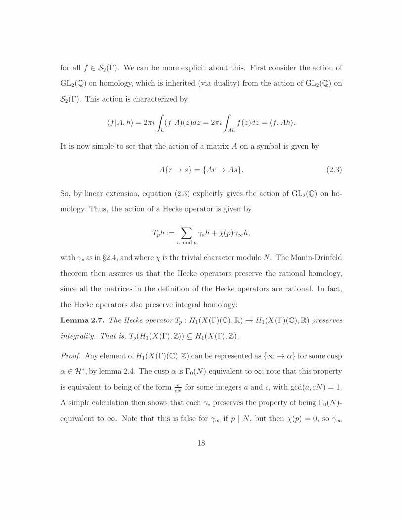
for all f ∈ S2(Γ). We can be more explicit about this. First consider the action of
GL2(Q) on homology, which is inherited (via duality) from the action of GL2(Q) on
S2(Γ). This action is characterized by
〈f |A, h〉 = 2πi
∫
h
(f |A)(z)dz = 2πi
∫
Ah
f(z)dz = 〈f, Ah〉.
It is now simple to see that the action of a matrix A on a symbol is given by
Ar → s = Ar → As. (2.3)
So, by linear extension, equation (2.3) explicitly gives the action of GL2(Q) on ho-
mology. Thus, the action of a Hecke operator is given by
Tph :=∑
a mod p
γah + χ(p)γ∞h,
with γ∗ as in §2.4, and where χ is the trivial character moduloN . The Manin-Drinfeld
theorem then assures us that the Hecke operators preserve the rational homology,
since all the matrices in the definition of the Hecke operators are rational. In fact,
the Hecke operators also preserve integral homology:
Lemma 2.7. The Hecke operator Tp : H1(X(Γ)(C),R) → H1(X(Γ)(C),R) preserves
integrality. That is, Tp(H1(X(Γ),Z)) ⊆ H1(X(Γ),Z).
Proof. Any element ofH1(X(Γ)(C),Z) can be represented as ∞ → α for some cusp
α ∈ H∗, by lemma 2.4. The cusp α is Γ0(N)-equivalent to ∞; note that this property
is equivalent to being of the form acN
for some integers a and c, with gcd(a, cN) = 1.
A simple calculation then shows that each γ∗ preserves the property of being Γ0(N)-
equivalent to ∞. Note that this is false for γ∞ if p | N , but then χ(p) = 0, so γ∞
18

need not be considered. Furthermore, γ∗ preserves ∞. Thus Tp∞ → α is a sum
of elements of H1(X(Γ)(C),Z), so is in that space.
The following theorem is essential, and is a consequence of lemma 2.7 when
k = 2:
Theorem 2.8. For any newform f ∈ Sk(Γ0(N)), the coefficients of f are algebraic
integers which generate a finite extension Kf of Q.
Proof. This is theorem 6.5.1 of [7], and the general proof is found there. The proof for
general k is analogous to the case k = 2, which will now be explained. First we check
that the Hecke operators generate a Z-subalgebra TZ of EndC(S2(Γ0(N))) that is
finitely generated and free as a Z-module. To do so, we take advantage of theorems
2.5 and 2.7 to view elements of TZ as endomorphisms of the finite free Z-module
H1(X(Γ)(C),Z). Thus TZ lies in the finite free Z-module EndZ(H1(X(Γ)(C),Z)), so
is itself finite and free.
The newform f then gives rise to an algebra homomorphism η : TZ → C, defined
by
Tn 7→ an(f).
It follows that the Z-subalgebra of C generated by the coefficients of f , which is
simply η(TZ), is finitely generated as a Z-module; thus all the coefficients of f are
algebraic integers, and they generate a finite extension of Q.
19

2.5.1 Sign decomposition
The duality in theorem 2.5 can be refined somewhat if we decompose the spaces
occuring there into real and imaginary parts first. Define
c :=
1 0
0 −1
.
The matrix c acts on H∗ via z 7→ −z. This gives an action of c on S2(Γ0(N)), given
by f ∗(z) = f(z∗). The eigenspaces for +1 and −1 are then respectively denoted
S2(Γ0(N))R and iS2(Γ0(N))R; implied in this notation is that S2(Γ0(N))R is the
subspace of cusp forms with real Fourier coefficients, and iS2(Γ0(N))R is that with
purely imaginary coefficients. Take H±1 (X(Γ0(N))(C),R) to be the ±1-eigenspace
for the action of c in homology; here c acts on homology via symbols, as described
earlier. Then the refined duality is given by:
Theorem 2.9. The integration pairing S2(Γ0(N))R ×H+1 (X(Γ0(N))(C),R) → R is
an exact pairing of R-vector spaces.
The proof of this and further details can be found in §2.1.3 of [5]. It is sim-
ple to see that c commutes with any Tp, so the Hecke operators respect the sign
decomposition.
2.6 Hecke module structure
The purpose of this section is to give an explicit description of S2(Γ0(N)), and
of the action of the Hecke operators on that space. There are two tools essential to
describing S2(Γ0(N)): the first is the duality of S2(Γ0(N)) and H1(X(Γ0(N))(C),R),
20

which was described in the previous section. The second is the Petersson scalar
product, which will now be defined.
Let F denote a fundamental domain for Γ0(N). Let
dµ(x+ yi) =dx dy
y2
be the hyperbolic measure on H. Define
VΓ0(N) =
∫
Fdµ(z).
The Petersson scalar product is defined by
〈f, g〉 := 1
VΓ0(N)
∫
Ff(z)g(z)ℑ(z)kdµ(z)
for f, g ∈ Sk(Γ0(N)). A simple calculation shows that the integrand is invariant
under the action of Γ0(N), which implies the well-definedness of the Petersson scalar
product. See §5.4 of [7] for details. We have the following important property
(theorem 5.5.3 of [7]):
Theorem 2.10. The Hecke operators Tn with n prime to N are self-adjoint with
respect to the Petersson scalar product. That is,
〈f, Tng〉 = 〈Tnf, g〉
for all f, g ∈ Sk(Γ0(N)), whenever n is prime to N .
Theorem 2.10 allows us to use results from linear algebra to describe a basis for
Sk(Γ0(N)) with nice properties (theorem 5.5.4 of [7]):
21

Theorem 2.11. The vector space Sk(Γ0(N)) has an orthogonal basis of simultaneous
eigenvectors for all of the Hecke operators Tn with n prime to N .
The ideal situation would be for the Hecke operators to cut out one-dimensional
eigenspaces. Unfortunately, this is not the case, but Atkin-Lehner theory allows us
to say more.
2.6.1 Atkin-Lehner theory
This section follows the work in the paper [2] of Atkin and Lehner. Atkin-
Lehner theory gives us constructions for changing the level of a cusp form. These
constructions allow us to decompose Sk(Γ0(N)) into Hecke-stable subspaces. The
decomposition aids greatly in the study of the Hecke module structure on Sk(Γ0(N)).
Lemma 2.12. Suppose Md | N for positive integers M and d. Let
δd :=
d 0
0 1
.
Then for g(z) ∈ Sk(Γ0(M)), we get g|δd ∈ Sk(Γ0(N)).
Proof. By direct calculation, for any
a b
Nc e
∈ Γ0(N),
we calculate
δd
a b
Nc e
δ−1d =
a db
Nc/d e
=
a db
Mc e
∈ Γ0(M).
22

So if we let f := g|δd and take γ ∈ Γ0(N), we get
f |γ = g| δd γ = g| δd γ δd−1 | δd = g|δd = f,
since δd γ δ−1d ∈ Γ0(M) by the above calculation. So f is a modular form with respect
to Γ0(N).
Define Sk(Γ0(N))old to be the subspace of Sk(Γ0(N)) spanned by f |δd for all
choices of M and d with Md | N , and all choices of cusp forms f of level M < N .
Take Sk(Γ0(N))new to be the orthogonal complement of Sk(Γ0(N))old with respect to
the Petersson scalar product. We then have
Sk(Γ0(N) = Sk(Γ0(N))new ⊕ Sk(Γ0(N))old.
Furthermore, theorem 5.6.2 in [7] tells us that the Hecke operators preserve the spaces
Sk(Γ0(N))new and Sk(Γ0(N))old. We can now make theorem 2.11 more specific:
Theorem 2.13. The space Sk(Γ0(N))new has an orthogonal basis of normalized cusp
forms that are eigenvectors for all of the Tn.
A member of this basis is called a newform. More generally, a cusp form f that is
an eigenvector for Tn for all positive integers n is called an eigenform. An important
consequence of theorem 2.3 is that for a normalized eigenform f , the eigenvalue
for Tn is an, since a1(Tnf) = an(f) and a1(f) = 1. Thus a normalized eigenform
is completely determined by its eigenvalues for the Hecke operators. So theorem
2.13 implies that the Hecke operators decompose Sk(Γ0(N))new into one dimensional
eigenspaces.
23
Theorem 2.13 can also be used to give an explicit description of a basis for
Sk(Γ0(N)) (theorem 5.8.3 of [7]):
Theorem 2.14. The set
f(dz) : f is a newform in Sk(Γ0(M))new, Md | N
is a basis for Sk(Γ0(N)).
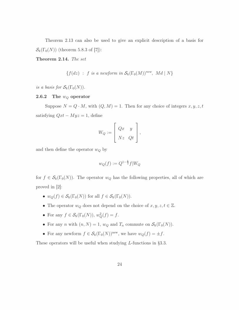
2.6.2 The wQ operator
Suppose N = Q ·M , with (Q,M) = 1. Then for any choice of integers x, y, z, t
satisfying Qxt−Myz = 1, define
WQ :=
Qx y
Nz Qt
,
and then define the operator wQ by
wQ(f) := Q1− k2 f |WQ
for f ∈ Sk(Γ0(N)). The operator wQ has the following properties, all of which are
proved in [2]:
• wQ(f) ∈ Sk(Γ0(N)) for all f ∈ Sk(Γ0(N)).
• The operator wQ does not depend on the choice of x, y, z, t ∈ Z.
• For any f ∈ Sk(Γ0(N)), w2Q(f) = f .
• For any n with (n,N) = 1, wQ and Tn commute on Sk(Γ0(N)).
• For any newform f ∈ Sk(Γ0(N))new, we have wQ(f) = ±f .
These operators will be useful when studying L-functions in §3.3.
24

2.7 Calculating spaces of cusp forms
The discussion in §2.6 outlines an interesting idea, which is the basis for many
algorithms used to calculate spaces of cusp forms. The idea is to go through the
discussion in reverse order. That is, we start by computing H1(X(Γ0(N))(C),Q),
which can be accomplished with simple algebra (as outlined in the proof of theorem
2.1.4 of [5]). The Hecke action is then computed on the rational homology, and is
linearly extended to H1(X(Γ0(N))(C),R). Now we can simply define S2(Γ0(N)) to
be the module HomR(H1(X(Γ0(N))(C),R),C), which inherits the Hecke-action from
homology. (Note that it is nicer if we split into real and imaginary spaces first; that
is, S2(Γ0(N))R is the R-dual of H+1 (X(Γ0(N)),R), and S2(Γ0(N)) = S2(Γ0(N))R ⊕
iS2(Γ0(N))R.) This gives an effective algorithm for computing the Hecke-module of
cusp forms.
To give a more explicit explicit description, we must calculate the q-expansions
of our cusp forms. To do so, we use Atkin-Lehner theory to cut out the subspace
S2(Γ0(N))new of S2(Γ0(N)). Then the Hecke operators decompose S2(Γ0(N))new
into 1-dimensional eigenspaces. For each eigenspace, the q-expansion of the corre-
sponding newform is then obtained by packaging the Hecke-eigenvalues into a formal
q-expansion.
2.8 Ordinary submodule
Let p denote a fixed prime greater than 3. This section will define the p-ordinary
submodule of the space Sk(Γ0(N)). Regardless of level, we take
Up :=
p−1∑
a=0
γa
25

with the matrices γ∗ defined as in section 2.4:
γa =
1 a
0 p
for a ∈ Z, γ∞ =
p 0
0 1
,
and
δd :=
d 0
0 1
.
Here we are considering Up as an operator on Sk(Γ0(N)) with varying level N . Note
that the Hecke operator on Sk(Γ0(N)) corresponding to the prime p is Up+χN(p)δp,
where χN is the trivial Dirichlet character modulo N .
For the next definition, we will need the following lemma:
Lemma 2.15. Suppose a ∈ Q is an algebraic integer. Recall that we have fixed an
embedding Q → Cp. In Cp,
limn→∞
an! =
1 if a is a unit
0 if a is a non-unit.
Proof. If a is not a unit, then it has positive (additive) p-adic valuation; thus the
limit of an! is clearly 0. So suppose a is a unit contained in the ring of integers O of
a finite extension K of Qp. Take a prime ideal p ⊆ O above pZp. Now a is a unit, so
by basic number theory,
a|O/pk |−1 ≡ 1 (mod pk).
For n large enough, |O/pk| − 1 divides n!, so the desired result follows by taking the
limit n→ ∞.
26

Hida’s projector to the ordinary part is defined as
eord = limn→∞
Un!p .
An eigenform for Γ0(N) is called ordinary at p if its Up-eigenvalue is a p-adic unit.
Lemma 2.15 tells us that an eigenform f is fixed by eord exactly if it is ordinary, and
otherwise eord maps f to 0. The ordinary submodule of Sk(Γ0(N)) is
Sordk (Γ0(N)) := eordSk(Γ0(N)).
To describe the ordinary submodule (and to prove well-definedness), we will consider
the action of the operator eord on a basis for Sk(Γ0(N)). The following lemma is
needed:
Lemma 2.16. If p ∤ d, then the operators δd and Up commute on S(Γ0(N)) for any
positive integer N . Also, δpUp acts as pk−1 on S(Γ0(N)).
Proof. A simple calculation shows that
δdUp = δd
(
p−1∑
a=0
γa
)
=
(
p−1∑
a=0
γda
)
δd = Upδd
since the action of γa only depends on a modulo p (as mentioned in section 2.4), and
d is prime to p. Also, recalling that scalar matrices act via the (k − 2) power map,
we get:
δpUp = δp
(
p−1∑
a=0
γa
)
=
p−1∑
a=0
p pa
0 p
= pk−2
p−1∑
a=0
1 a
0 1
,
which acts as pk−1.
27

Note that lemma 2.16 implies that eord commutes with δd if p ∤ d. Theorem 2.14
gives the following basis for Sk(Γ0(N)):
f |δd : f is a newform in Sk(Γ0(N′))new, dN ′ | N .
The following lemma gives the action of eord on members of this basis:
Lemma 2.17. Suppose d and N ′ are positive integers such that dN ′ | N , and suppose
f is a newform of level N ′. If ap(f) is not a p-adic unit, then
eord(f |δd) = 0.
If ap(f) is a p-adic unit, let α, β be the roots of Frobenius of f ; that is, the roots of
x2 − ap(f)x+ χN ′(p)pk−1. Assume the roots are ordered so that α is a unit and β is
a non-unit. Then
eord(f |δd) =α
α− β(f |δd − βp1−kf |δpd)
if (p, d) = 1, and
eord(f |δd) =pk−1
α− β(f |δd/p − βp1−kf |δd)
if p | d.
Proof. Note that δaδb = δab, so δa and δb always commute. Note also that δd com-
mutes with eord when (p, d) = 1, since δd commutes with Up. Thus we can assume
without loss of generality that d = 1 or p. We have, since f is a newform at level
N ′, that
f |(Up + χN ′(p)δp) = apf,
28
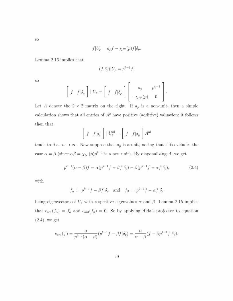
so
f |Up = apf − χN ′(p)f |δp.
Lemma 2.16 implies that
(f |δp)|Up = pk−1f,
so[
f f |δp]
| Up =[
f f |δp]
ap pk−1
−χN ′(p) 0
.
Let A denote the 2 × 2 matrix on the right. If ap is a non-unit, then a simple
calculation shows that all entries of A2 have positive (additive) valuation; it follows
then that[
f f |δp]
| Un!p =
[
f f |δp]
An!
tends to 0 as n → ∞. Now suppose that ap is a unit, noting that this excludes the
case α = β (since αβ = χN ′(p)pk−1 is a non-unit). By diagonalizing A, we get
pk−1(α− β)f = α(pk−1f − βf |δp)− β(pk−1f − αf |δp), (2.4)
with
fα := pk−1f − βf |δp and fβ := pk−1f − αf |δp
being eigenvectors of Up with respective eigenvalues α and β. Lemma 2.15 implies
that eord(fα) = fα and eord(fβ) = 0. So by applying Hida’s projector to equation
(2.4), we get
eord(f) =α
pk−1(α− β)(pk−1f − βf |δp) =
α
α− β(f − βp1−kf |δp).
29

Similarly,
(α− β)f |δp = (pk−1f − βf |δp)− (pk−1f − αf |δp),
so
eord(f |δp) =pk−1
(α− β)(f − βp1−kf |δp).
Definition 2.18. Suppose f ∈ Sk(Γ0(N)) is a p-ordinary cusp form which is an
eigenvector for Tp, and let β denote its non-unit root of Frobenius at p. The p-
stabilized cusp form g corresponding to f is the cusp form
g := f − βp1−kf |δp,
which satisfies
g(z) = f(z)− βf(pz).
Note that the if p divides N , then β = 0, so f is already p-stabilized. Otherwise,
g ∈ Sk(Γ0(Np)).
Corollary 2.19. The space Sord
k (Γ0(N)) has basis
B = f(dz)− βf(pdz) : f is a p-ordinary newform in Sk(Γ0(N′))new,
(p, d) = 1, dN ′ | N,
where β denotes the non-unit root of Frobenius of f at p.
Proof. Lemma 2.17 implies that B spans the ordinary subspace, since every basis
element for Sk(Γ0(N)) (from theorem 2.14) maps to a multiple of an element of B
30
under eord. Linear independence follows from the linear independence of the basis in
theorem 2.14.
31
CHAPTER 3L-functions and modular symbols
The L-function of a cusp form f is an analytic function which encodes the
Fourier coefficients of f . Values of the L-function can be expressed in terms of
modular symbols. Modular symbols encode line integrals along geodesic paths in
the upper half plane. These symbols greatly aid the computation of the values of L-
functions since the calculation of modular symbols can be reduced to linear algebra.
Modular symbols are also indispensable when defining p-adic L-functions.
3.1 Modular symbols
Define
∆0 = Div0(P1(Q)) :=
∑
r∈S⊂P1(Q)
ar · [r]∣
∣
∣
∣
∣
ar ∈ Z, S finite ,∑
r∈Sar = 0
to be the group of degree 0 divisors. Also, let ∆0(R) := ∆0 ⊗ R. For an abelian
group A, we define the space of A valued symbols
Symb(A) := φ : ∆0 → A
to be the abelian group of homomorphisms from ∆0 to A. Now suppose Γ is a
subgroup of SL2(Z) or PSL2(Z). The group Γ then acts on ∆0 (on the left) by linear
fractional transformations, as defined in chapter 2. If A is a right Γ-module, we
32
define a right action of Γ on Symb(A) by the rule:
(φ|γ)(D) = φ(γD)|γ.
Then we define
SymbΓ(A) :=
φ ∈ Symb(A) such that φ(γD) = φ(D)|γ−1 ∀γ ∈ Γ
to be the Γ invariant subspace of Symb(A). For a modular symbol φ and r, s ∈ P1(Q),
we will use the notation
φr → s
to denote the value of φ at the divisor [s]− [r].
3.1.1 Modular symbols attached to a cusp form
Define Pk(K) to be the set of homogeneous polynomials in two variables of
degree k− 2, with coefficients in the field K. Let Vk(K) denote the K-linear dual of
Pk(K). There is a natural right action of GL2(K) on Pk(K) given by
(P |A)(x, y) := P (ax+ by, cx+ dy) for A =
a b
c d
(Note that scalar matrices act via the k − 2 power map.) This action gives rise to a
right action of GL2(K) on Vk(K) given by (v|A)(P ) = v(P |A) for v ∈ Vk(K) (recall
that A = det(A)A−1). To a cusp form f ∈ Sk(Γ0(N)), we attach the Vk(C)-valued
symbol If defined by
Ifr → s(P ) := 2πi
∫ s
r
f(z)P (z, 1)dz.
33

The path of integration is the geodesic path connecting the cusp r to s, with the
hyperbolic metric (as described in section 2.6). A note should be made about con-
vergence:
Lemma 3.1. For a cusp form f ∈ Sk(Γ0(N)), the integral
∫ s
r
f(z)g(z)dz
converges absolutely for any polynomial g.
Proof. Pick an arbitrary point α ∈ H along r → s. The group SL2(Z) acts
transitively on the cusps, so there is a matrix A such that A∞ = s. By a change of
variables z 7→ Az and by equation (2.2),
∫ s
α
f(z)g(z)dz =
∫ ∞
A−1α
f(Az)g(Az)d(Az)
=
∫ ∞
A−1α
(f |A)(z)j(A, z)k−2g(Az)dz. (3.1)
Note that the path of integration is a vertical line for the last integral. The form f
is cuspidal, so by definition, (f |A)(z) has a Fourier expansion with which contains
only positive powers of q = e2πiz. Thus as ℑ(z) → ∞, the absolute value of (f |A)(z)
tends to 0 exponentially. Also, j(A, z)k−2g(Az) has subexponential growth, so the
integral on the right of equation (3.1) converges absolutely. Similarly, the integral
from r to α converges absolutely, so the integral from r to s converges.
The modular symbol If has two important properties:
• If ∈ SymbΓ0(N)(Vk(C)) (i.e. it is invariant under the action of Γ0(N).)
• If is C-linear in f .
34

The first of these follows from the corollary to the following lemma, and the second
is clear from the definition.
Lemma 3.2. for A ∈ GL+2 (R) (i.e. a 2 × 2 real matrix with positive determinant),
we have
If |Ar → s(P |A) := det(A)k−2IfAr → As(P )
Corollary 3.3.
If |A = If |A
Corollary 3.4. If is invariant under Γ0(N).
Proof. By a simple calculation (done in section 2.2),
d(Az) = d
(
az + b
cz + d
)
= det(A)(cz + d)−2dz (3.2)
so
(f |A)(z)(P |A)(z, 1)dz
= det(A)k−1(cz + d)−kf(Az)P (az + b, cz + d)dz
= det(A)k−1(cz + d)−kf(Az)(cz + d)k−2P
(
az + b
cz + d, 1
)
dz
= det(A)k−2f(Az)P (Az, 1) det(A)(cz + d)−2dz
= det(A)k−2f(Az)P (Az, 1)d(Az),
35
and hence
If |Ar → s(P |A) = 2πi
∫ s
r
(f |A)(z)(P |A)(z, 1)dz
= 2πi det(A)k−2∫ s
r
f(Az)P (Az, 1)d(Az)
= 2πi det(A)k−2∫ As
Ar
f(z)P (z, 1)dz
= det(A)k−2IfAr → As(P ).
The corollary then follows easily:
(If |A)r → s(P ) = ((If Ar → As)|A)(P )
= If Ar → As (P |A)
= det(A)2−kIf |A r → s (P |AA)
= det(A)2−k det(A)k−2If |A r → s (P )
= If |A r → s (P ),
noting that
AA =
detA 0
0 detA
.
3.1.2 Action of the Hecke operators
Recall the following notation from section 2.4: for a prime p, we take
γa =
1 a
0 p
for 0 ≤ a ≤ p− 1, γ∞ =
p 0
0 1
.
36

We define the Hecke operators on modular symbols as follows for a right Γ0(N)-
module A (with χ being the trivial character modulo N):
I|Tp := I
∣
∣
∣
∣
∣
(
∑
a mod p
γa + χ(p)γ∞
)
(3.3)
for I ∈ SymbΓ0(N)(A), so that corollary 3.3 implies that
If |Tp = If |Tp.
3.1.3 Sign decomposition
The section is analogous to §2.5.1. The matrix
c :=
1 0
0 −1
normalizes Γ0(N), by a simple calculation. The matrix c thus induces an involution
on SymbΓ0(N)(Vk(C)), sending I to I|c; note then that for all γ ∈ Γ0(N)
I|cγ = I|(cγc−1)c = I|c,
so I|c is Γ0(N)-invariant. We can decompose If into the sum of its eigencomponents:
If = I+f + I−f , where I+f =If + If |c
2, I−f =
If − If |c2
.
Suppose the coefficients of the q-expansion of f generate the number field Kf (re-
calling theorem 2.8), with ring of integers Of . A theorem of Hatada (theorem 3 of
[12]) implies the following:
37

Theorem 3.5. There exist periods Ω+ and Ω− such that the symbols defined by
φ±f := (Ω±)−1I±f
take values in Vk(Of ).
Theorem 3.5 will be essential when trying to interpolate modular symbols p-
adically. The symbol φ±f will be referred to as the normalized modular symbol at-
tached to f of sign ±1.
3.2 Explicit description
This section will explain a result of Manin which gives an explicit description
of a modular symbol space. To do so for a subgroup Γ ⊆ G := PSL2(Z), we need a
description of ∆0 as a Γ-module. There is a map from G to ∆0 defined by
a b
c d
7→[
a
c
]
−[
b
d
]
.
We extend this linearly to a map
d : Z[G] → ∆0.
A result of Manin, found in §2.2 of [19], states the following:
Theorem 3.6. The map d defined above is surjective. The kernel is
I = Z[G](1 + τ + τ 2) + Z[G](1 + σ)
where
τ =
0 −1
1 −1
, σ =
0 −1
1 0
,
38

which are 3 and 2-torsion elements respectively.
Theorem 3.6 gives rise to a complete (though complicated) description of the
Γ-module ∆0, since Z[G] is a free Z[Γ]-module; if G =r⊔
i=1
Γgi, then
Z[G] =
r⊕
i=1
Z[Γ]gi.
To describe ∆0 as a Γ-module, we translate the relations from theorem 3.6 into
relations among the gi. For example,
gi(1 + σ) = gi + γijgj
where gj is the right coset representative for giσ for each i. There are similar relations
for τ . In principle, this could be sufficient to describe any Γ-homomorphism from ∆0,
but to do so, we would have to simultaneously solve many equations in the target
space. So realistically, we need a more explicit description to continue. The approach
of Pollack and Stevens [19] will be outlined in section 5.8.
3.3 The L-function attached to a cusp form
Suppose f ∈ Sk(Γ0(N)) has q-expansion
f(z) =∑
n≥1anq
n, q = e2πiz.
The L-series attached to f is defined by
L(f, s) :=∑
n≥1ann
−s
for s such that ℜ(s) > k2+ 1.
39
Lemma 3.7. The L-series attached to f has the following integral representation:
L(f, s) =(2π)s
Γ(s)
∫ ∞
0
f(it)tsdt
t
for s with ℜ(s) > k2+1. Furthermore, the L-series extends to a holomorphic function
on the whole complex plane, called the L-function attached to f .
Proof. This is found in §5.10 of [7]; an outline will be presented here. The integral
representation is verified by expanding f into its q-expansion, then integrating term
by term. The argument in the proof of lemma 3.1 can be applied here to show that
the integral above is in fact absolutely convergent for any value of s ∈ C. Also, Γ(s)−1
is well known to be an entire function, so L(f, s) extends to an entire function.
Corollary 3.8. For integer values of j in the range 1 ≤ j ≤ k − 1,
L(f, j) =(−2πi)j−1
(j − 1)!If∞ → 0(xj−1yk−j−1).
Proof. Using lemma 3.7:
If0 → ∞(xj−1yk−j−1) = 2πi
∫ ∞
0
f(z)zj−1dz
= 2πi
∫ ∞
0
f(it)(it)j−1d(it)
= 2πij+1
∫ ∞
0
f(it)tjdt
t
= − (j − 1)!
(−2πi)j−1L(f, j).
40
The values of L(f, j) for j in the range 1 ≤ j ≤ k − 1 are called the critical
values of L(f, s). Corollary 3.8 expresses these critical values in terms of the modular
symbol attached to f . In fact, a similar result also holds if we twist f by a Dirichlet
character.
3.3.1 Twists
For a modular form f , the twist of f by a Dirichlet character χ is defined to be
fχ(z) :=
∞∑
n=0
χ(n)anqn
The function fχ can be expressed in terms of the original function f as follows. For
simplicity, we assume χ is a primitive character of conductor m. Define the usual
Gauss sums as
τ(n, χ) =∑
a mod m
χ(a)e2πina/m, τ(n) = τ(1, χ)
The following calculation will allow us to give a different representation of fχ:
Lemma 3.9. τ(n, χ) = χ(n) · τ(χ) for n prime to m.
Proof.
τ(n, χ) =∑
a mod m
χ(a)e2πina/m
= χ(n)∑
a mod m
χ(na)e2πina/m
= χ(n)∑
a mod m
χ(a)e2πia/m = χ(n) · τ(χ)
where the last line follows since (m,n) = 1, so n 7→ an is a bijection modulo m.
Lemma 3.9 can then be used to obtain the aforementioned representation of fχ:
41

Lemma 3.10 (Birch’s Lemma). Suppose f is a modular form in Γ0(N), and χ is a
primitive character of conductor m. Then
fχ =1
τ(χ)
∑
a mod m
χ(a)f
∣
∣
∣
∣
∣
∣
∣
1 a/m
0 1
.
Proof. By lemma 3.9,
fχ(z) =∑
n
χ(n)ane2πinz =
∑
n
τ(n, χ)
τ(χ)ane
2πinz
=1
τ(χ)
∑
n
∑
a mod m
χ(a)e2πina/mane2πinz
=1
τ(χ)
∑
a mod m
χ(a)∑
n
ane2πin(z+a/m)
=1
τ(χ)
∑
a mod m
χ(a)f(
z +a
m
)
Now consider a primitive character χ modulo m. Birch’s lemma (lemma 3.10)
gives the twisting rule, where
δa =
1 a/m
0 1
is the matrix in that lemma:
Ifχ r → s (P ) = 1
τ(χ)
∑
a mod m
χ(a)If |δa r → s (P )
=1
τ(χ)
∑
a mod m
χ(a)If δar → δas (P |δ−a),
42

where we use lemma 3.2 for the last step, and note that δa = δ−a. Now corollary 3.8
tells us that for 1 ≤ j ≤ k − 1:
L(fχ, j) =(−2πi)j−1
(j − 1)!Ifχ ∞ → 0 (xj−1yk−j−1)
=(−2πi)j−1
(j − 1)! τ(χ)
∑
a mod m
χ(a)If
∞ → a
m
(
(
x− a
my)j−1
yk−j−1)
.
Thus all the special values of all twists of the L-function of f can be expressed in
terms of the values of the modular symbol If .
3.4 The functional equation
The L-function attached to a newform satisfies a certain functional equation.
Among other uses, this functional equation allows us to study the order of vanishing
of the L-function at the central critical point. To state the functional equation, it is
convenient to first multiply the L-function by some additional factors:
Definition 3.11. For a cusp form f ∈ Sk(Γ0(N)), we set
Λ(f, s) := Ns2
∞∫
0
f(it)tsdt
t= N
s2 (2π)−sΓ(s)L(f, s),
recalling lemma 3.7.
Now recall the wQ operator from section 2.6.2. Recall also the fact that any
newform of level N is an eigenvector for the wN operator.
Theorem 3.12. For f ∈ Sk(Γ0(N)), the following relation holds:
Λ(wN(f), s) = i−kΛ(f, k − s).
43

Corollary 3.13. Suppose f ∈ Sk(Γ0(N)) is an eigenvector for the wN operator, with
eigenvalue c = ±1, then
Λ(f, s) = ci−kΛ(f, k − s).
The parity of the order of vanishing n of Λ(f, s) at s = k2
is determined by
c = (−1)n−k2 .
Proof. By definition,
wN(f)(z) = N1− k2
f
∣
∣
∣
∣
∣
∣
∣
0 −1
N 0
(z) = N−
k2 z−kf
(−1
Nz
)
,
so
Λ(wN(f), s) = Ns2
∞∫
0
(wNf)(it)tsdt
t
= Ns2− k
2 i−k∞∫
0
f
( −1
Nit
)
ts−kdt
t
which, by the change of variable u = 1Nt
, gives
Λ(wN(f), s) = Nk−s2 i−k
∞∫
0
f(iu)uk−sdu
u
= i−kΛ(f, k − s).
The corollary follows from considering the Taylor expansion of Λ(f, s) around s = k2.
If the order of vanishing of Λ(f, s) is n at s = k2, then the functional equation tells
44

us, by taking nth coefficients on each side, that
c = i−k(−1)n = (−1)n−k2 .
In fact, there is also a functional equation for twists of L-functions attached to
cusp forms. The proof is largely similar, although the details of the calculation are
more involved, so will be omitted.
Theorem 3.14. Suppose f ∈ Sk(Γ0(N)) is a wN -eigenvector with eigenvalue c, and
ψ is a primitive Dirichlet character of conductor m which is relatively prime to N .
The following relation holds:
τ(ψ)−1Λ(fψ, s) = cNk2−s ψ(−N) τ(ψ)−1Λ(fψ, k − s),
where τ(ψ) denotes the Gauss sum associated to ψ.
Note that for a quadratic Dirichlet character ψ, we have ψ = ψ, so we can again
use the functional equation to determine the order of vanishing of the L-function at
the central critical point.
45

CHAPTER 4Elliptic Curves
One of the central interests in number theory is the solution of polynomial
equations over Q. Unfortunately, this problem becomes difficult very quickly as the
degrees of the polynomials increase. For quadratic equations, the solution is made
easier by the fact that the Hasse principle holds:
Definition 4.1. A class of algebraic varieties defined over a number field K is said
to satisfy the Hasse principle if, for each variety V in the class,
V (K) 6= ∅ ⇔ V (Kν) 6= ∅ ∀ν,
where ν varies over all the places of K, and Kν is the localization at ν. Thus a
quadratic polynomial has a solution over Q if and only if it does modulo all prime
powers and in the real numbers. The Hasse principle fails for equations of degree
greater than 2, which makes the problem of finding solutions much harder. The case
of degree 3 equations reduces to the problem of finding points on elliptic curves.
This chapter gives an overview of some properties of elliptic curves that will be used,
following Silverman’s book [21].
4.1 Definition
Definition 4.2. An elliptic curve over a field K is a pair (E,O), with E a smooth
projective curve of genus 1 over K, and O ∈ E(K).
46

Generally an elliptic curve (E,O) will be denoted simply E, with O being un-
derstood from the context. Every elliptic curve can be written in Weierstrass form:
E is the set of (projective) solutions to the equation:
y2 + a1yx+ a3y = x3 + a2x2 + a4x+ a6 (4.1)
for some constants a1, a2, a3, a4 and a6 inK, with the distinguished point O being the
point at infinity. It is useful to more generally consider curves defined by equations
of the form (4.1) that give rise to possibly singular (i.e. non-smooth) curves. There
are several important quantities related to the curve E: the discriminant ∆ of the
curve E is a quantity which vanishes iff E is singular; another quantity, denoted c4,
is important when ∆ = 0 (that is, when E is singular). The quantities ∆ and c4
are both defined as polynomials in the coefficients ai, with integer coefficients. The
formulae defining ∆ and c4 can be found in [21], §III.
Note that E is singular iff there is a point on E for which the Jacobian matrix
related to the Weierstrass equation has less than full rank. When E is singular, it is
simple to check that there is exactly one singularity. There are two possible behaviors
for an elliptic curve at a singularity; either there are two tangent directions, or there
is only one. A singularity is called a node in the case of two tangent directions, which
occurs if c4 6= 0, and is called a cusp when there is only one tangent direction, which
occurs if c4 = 0.
4.2 Group Structure
Now we consider the set E(K) of points on E defined over K. Given points
P,Q ∈ E(K), we define P ⋆ Q to be the third point of intersection with E of the
47
line passing through P and Q. An elementary computation shows that P ⋆ Q also
lies on E(K). Then we define addition on the curve by P + Q = O ⋆ (P ⋆ Q). This
compositon law can be proven to be commutative and associative, with O as the
identity element. The set E(K) thus has an abelian group structure, and much work
has gone into describing its properties.
A crucial result is the Mordell theorem, which can be found in Chapter VIII
of [21]: for a number field K, the Mordell theorem tells us that the group E(K) is
finitely generated. Thus the structure theorem for abelian groups tells us that
E(K) ∼=k∏
i=1
Z
niZ× Zr (4.2)
for some positive integers n1, . . . , nk and r. The integer r is called the rank of E(K).
So Mordell’s theorem tells us that the rank of E(K) is finite for any number field
K. Unfortunately, the proof of Mordell’s theorem is not effective, so the problem of
finding an algorithm to compute the group structure of E(K) is still open.
4.3 Reduction modulo primes
Fix a prime p. Suppose E is an elliptic curve defined over Q by an equation of
the form 4.1 with integer coordinates. Take E to be the curve over Fp defined by the
modulo p reduction of the Weierstrass equation of E.
The quantities ∆, c4 corresponding to E can then be seen to be the reduction
modulo p of the quantities ∆, c4 related to E, since ∆ and c4 are integer polynomials
in the coefficients of the Weierstrass equation of E. We say E has
• good (or stable) reduction modulo p if ∆ 6= 0, i.e. p ∤ ∆
48
• bad reduction of multiplicative type (or is semi-stable) if ∆ = 0, and the
singularity is a node (i.e. c4 6= 0)
• bad reduction of additive type (or is unstable) if ∆ = 0, and the singularity is
a cusp (i.e. c4 = 0)
Further, if E has multiplicative reduction, we say that the reduction is split if the
tangent slopes at the singularity lie in Fp, and that the reduction is non-split other-
wise. The determinant ∆ encapsulates information about the reduction of E modulo
all of the primes. That said, ∆ does not distinguish between different types of bad
reduction; the conductor is a quantity similar to ∆ which encodes extra information
about the reduction of E. The conductor of E is defined as
nE :=∏
p prime
pfE(p)
where, for p > 3, the exponent fE(p) is 0 if E has good reduction modulo p, is 1 for
multiplicative reduction, and is 2 for additive reduction. For p = 2 or p = 3, the
formula is slightly more complicated; see [20] §IV.10 for more information about the
conductor. The conductor has the same prime divisors as the discriminant, though
the powers appearing in the conductor are always small.
Given a point P = [X, Y, Z] ∈ P2(Q), we can always rescale the coordinates so
that they are relatively prime integers; the resulting coordinates will be called reduced
coordinates for P . Suppose P is a projective point on E with reduced coordinates
[X, Y, Z]. The reduction of P modulo the prime p gives a point P in P2(Fp), since
not all coordinates of P are 0 modulo p (lest the coordinates share a common factor).
The point P can easily be seen to lie on E. So we get a map E → E; thus we can
49
extract information about E over Q by analyzing the curve E defined over the finite
field Fp, since any rational point on E is a lift of a point in E.
4.4 The L-function attached to an elliptic curve
Recall that in the case of a quadratic equation, the problem of determining
whether a rational solution exists is made easier by the validity of Hasse’s principle;
that is, the fact that the equation need only be solved modulo prime powers and
in R. If a solution is found, it is then easy to find all the others, by projecting
onto a line. Unfortunately, Hasse’s local-global property fails to hold in the cases of
degree higher than 2. In the case of an elliptic curve E, the Birch and Swinnerton-
Dyer conjectures suggest that global information can be gleaned from the combined
local information, despite the failure of Hasse’s principle. There is strong numerical
evidence in support of the Birch and Swinnerton-Dyer conjectures.
To study the local properties of a rational elliptic curve E, the following functions
are defined: the local zeta function of a rational elliptic curve E at a prime p of good
reduction is
Zp(E, z) = exp
( ∞∑
n=1
#E(Fpn)
nzn
)
.
The local zeta function can be shown to be a rational function. More specifically, in
§C.16 of [21], the following is shown:
Zp(E, z) =Lp(z)
(1− z)(1 − pz)
with Lp(z) = 1 − apz + pz2. The ap in this equation is equal to p + 1 − #E(Fp).
In the case of bad reduction, we define Lp(z) = 1 − apz, with ap being 0 in the
50

case of additive reduction, 1 for split multiplicative reduction and −1 for non-split
multiplicative reduction.
The zeta functions encode all the information about E modulo prime powers.
We combine this local information into the following object, called the Hasse-Weil
L-function attached to the elliptic curve E:
L(E, s) :=∏
p
Lp(p−s)−1 =
∏
p∤∆
(1− app−s + p1−2s)−1 ·
∏
p|∆Lp(p
−s)−1.
A theorem of Hasse ensures that |ap| ≤ 2√p, which implies that this function con-
verges for ℜ(k) > 32. The product defining L(E, s) can be expanded into an L-series :
L(E, s) :=∑
n≥1ann
−s,
which will converge on the same half-plane. The modularity theorem, which is de-
scribed in §4.5, implies that L(E, s) extends to be holomorphic on the whole complex
plane.
In the case of an elliptic curve E defined over a number field K, the L-function
L(E/K, s) can be defined similarly. See §II.10 of [20] for details of the construction
of L(E/K, s).
4.5 The Modularity Theorem
Starting with a rational modular form f for Γ0(N), a construction of Eichler and
Shimura associates to f a rational elliptic curve E of conductor N . The elliptic curve
E has the property that its L-function is equal to that of f . The Eichler-Shimura
construction and the aforementioned results are explained in §XI of [15] (see theorem
51

11.74). A natural question follows; do all elliptic curves arise from the Eichler-
Shimura construction? Shimura and Taniyama conjectured the affirmative answer
to this question for all rational elliptic curves. The Shimura-Taniyama conjecture
was proven in 2001 by the work of Breuil, Conrad, Diamond and Taylor [4], and
will be referred to as the modularity theorem for the rest of this thesis. The proof
of the modularity theorem was a continuation of a breakthrough of Wiles [27] and
of Taylor and Wiles [23], who proved the Shimura-Taniyama conjecture for a large
class of elliptic curves. The modularity theorem has far-reaching consequences, one
of which is a proof of Fermat’s Last Theorem, a problem which had stood unproved
for over 300 years. A concise but comprehensive summary of the Shimura-Taniyama
conjecture and its proof can be found in [6].
The modularity theorem is very useful for working with elliptic curves, and in
particular L-functions of elliptic curves, since modular forms are often easier to work
with directly. For example, the L-series of a cusp form can easily be shown to extend
to a holomorphic function on the entire complex plane, whereas that of an elliptic
curve is much more difficult to extend. In particular, the modularity theorem allows
us to extend the L-function of an elliptic curve to s = 1, so that the statement of
the Birch and Swinnerton-Dyer conjecture makes sense. The modularity theorem is
also useful when defining p-adic L-functions, again because modular forms are easier
to work with directly.
4.6 The Birch and Swinnerton-Dyer Conjecture
The Birch and Swinnerton-Dyer conjecture states that at s = 1, the Hasse-Weil
L-function L(E, s) attached to a rational elliptic curve E has order of vanishing equal
52
to the rank of E. Thus the BSD conjecture relates the global arithmetic properties
of the elliptic curve E to the analytic properties of the L-function L(E, s), which
encodes the local information about E. In fact, the Birch and Swinnerton-Dyer
conjecture has been generalized to say that even more information can be extracted
from the L-function. Specifically, a conjectural formula for the leading coefficient of
the Taylor series of L(E, s) around s = 1 is given, which expresses the coefficient as
a product of terms related to the arithmetic properties of E. The following version
of the Birch and Swinnerton-Dyer conjecture and a concise outline of the conjecture
can be found in Wiles’s article [26].
Conjecture 4.3 (The Birch and Swinnerton-Dyer Conjecture). The L-function
L(E, s) of an elliptic curve E has a Taylor expansion at s = 1 satisfying:
L(E, s) = c · (s− 1)r + higher order terms
and further,
c =ΩE ·∏ cp · |X(E/Q)| · Reg(E/Q)
|E(Q)torsion|2
All of the quantities appearing in this factorization are defined in terms of the
arithmetic properties of E. One of the most important partial results to date is the
following theorem of Kolyvagin, building on the work of Gross, Zagier and others
(which is discussed in [26]):
Theorem 4.4 (Kolyvagin’s Theorem). If L(E, s) vanishes to exact order 0 or 1 at
s = 1, then the Birch and Swinnerton-Dyer conjecture holds, i.e. the rank of E is
equal to the order of vanishing of L(E, s) at s = 1.
53

As for numerical evidence, Cremona (for example) has done computations for
large classes of rational elliptic curves, and the results have always been consistent
with the Birch and Swinnerton-Dyer conjecture. See [5] for more information on
Cremona’s work. Note that the modularity theorem is a big advancement in regards
to the Birch and Swinnerton-Dyer conjecture; it guarantees that the L-function of
a rational elliptic curve E is entire, so in particular, L(E, s) is analytic around
s = 1. The modularity theorem is also a big advancement since, prior to the proof,
many theorems (including Kolyvagin’s theorem) were only known to hold for modular
elliptic curves.
4.7 The Twisted Birch and Swinnerton-Dyer Conjecture
Take E to be an elliptic curve defined over Q, and suppose K/Q is a finite
abelian extension of Q with galois group G. It is possible to decompose the vector
space E(K) ⊗ Q into a direct sum, based on the action of G. It is also possible
to decompose the L-function L(E/K, s) into a product of “twisted” L-functions.
These decompositions can be matched up to provide a refinement of the Birch and
Swinnerton-Dyer conjecture. Kisilevsky and Fearnley [8, 9] and others have worked
on precise formulations of these refined conjectures, and have compiled numerical
evidence in their support. This section summarizes the work in [8], which provides
motivation for formulating new analogues of the Birch and Swinnerton-Dyer conjec-
tures, as will be done in §6.7.
The group G acts on E(K) by the following formula on Weierstrass coordinates:
P σ := (xσ, yσ) for P = (x, y) ∈ E(K).
54

Note that we assumed that E was defined over Q, so that P σ can easily be seen to lie
again on E(K) by applying σ to the Weierstrass equation. This action gives rise to
an action of G on E(K)⊗Q. Note that the Mordell theorem, in the form of equation
(4.2), implies that E(K)⊗Q is free over Q of dimension r equal to the rank of E(K)
(since the integers ni appearing in equation (4.2) are invertible). Define G to be the
group of characters χ of G; that is, homomorphisms χ : G→ Q×.
Definition 4.5. For a character χ ∈ G, the χ-part of E is
(E(K)⊗Q)χ := P ∈ E(K)⊗Q such that P σ = χ(σ)P ∀ σ ∈ G.
The χ-rank of E(K) is the Q-dimension of (E(K)⊗Q)χ, and is denoted rχ(E(K)).
It follows from the theory of representations of finite groups that we have a
decomposition
E(K)⊗Q =⊕
χ∈G
(E(K)⊗Q)χ.
From this it follows that
∑
χ∈G
rχ(E(K)) = r(E(K)).
The next step is to decompose the L-function L(E/K, s) into a product, with
each factor corresponding to an element of G. Using class field theory, we can
associate to any χ ∈ G a Dirichlet character, also denoted χ by abuse of notation.
The Dirichlet character χ has period D equal to the discriminant of K/Q. The
primitive Dirichlet character associated to χ will be denoted χ∗. Now we define
twists of L-functions by Dirichlet characters:
55
Definition 4.6. The L-series of E/Q twisted by a Dirichlet character ψ is the func-
tion
L(E, ψ, s) :=∑
n≥1ψ(n)ann
−s,
where
L(E, s) :=∑
n≥1ann
−s
is the L-series of E/Q. The holomorphic extension of L(E, ψ, s) to the whole complex
plane is called the L-function of E twisted by ψ.
This allows us to define twists by characters χ ∈ G:
Definition 4.7. The L-function of E/Q twisted by a character χ ∈ G is
L(E, χ, s) := L(E, χ∗, s)
where χ∗ is the primitive Dirichlet character associated to χ.
This definition allows us to decompose the function L(E/K, s) into a product:
Theorem 4.8.
L(E/K, s) =∏
χ∈G
L(E, χ, s).
The decompositions of L(E/K, s) and E(K)⊗Q lead to a natural generalization
of the Birch and Swinnerton-Dyer conjecture to the case of twisted L-functions:
Conjecture 4.9 (The Twisted Birch and Swinnerton-Dyer Conjecture). For an
abelian extension K/Q and a character χ : Gal(K/Q) → C×, the order of vanishing
of L(E, χ, s) at s = 1 is equal to the rank rχ of (E(K)⊗Q)χ.
56
In fact, Fearnley and Kisilevsky [8, 9] further provide a (conjectural) formula
for the leading coefficient of L(E, χ, s), which decomposes the formula found in con-
jecture 4.3. The authors also provide numerical data in support of their conjecture.
57
CHAPTER 5The p-adic L-function
The special values of L-functions twisted by characters can be interpolated p-
adically in different ways to give p-adic analogues of L-functions. This section will
outline the construction and computation of the Mazur-Swinnerton-Dyer p-adic L-
function, following the paper “On p-adic analogues of the conjectures of Birch and
Swinnerton-Dyer" by Mazur, Tate and Teitelbaum [17].
Throughout, Mk(N,χ) denotes the space of modular forms of weight k, level
Γ0(N) and character χ, and Sk(N,χ) is the corresponding space of cusp forms. We
fix a “sign at infinity” w∞ = ±1, and take φf to be the normalized modular symbol
attached to a cusp form f of sign w∞, which was introduced in §3.1.3. Finally, p will
denote a fixed prime greater than 3.
5.1 p-adic distributions
Let X be a compact open subset of Qnp for some n. A p-adic distribution on
X is a finitely additive function from the set of compact open subsets of X to a
vector space over Cp with an additive valuation ν. If a distribution µ is uniformly
bounded (i.e. ∃K ∈ R with ν(µ(U)) ≥ K for all compact open subsets U of X),
then µ is called a measure. There is an important difference between the concept of
distribution and measure; a priori, the notion of integrating a continuous function
against a distribution is not well defined unless the distribution is in fact a measure.
Nonetheless, as is explained in this chapter, a useful notion of integration can be
58
defined from some distributions. More information about distributions and measures
can be found in Washington’s book [25].
Fix a prime p and an eigenform f ∈ Sk(N,χ) of Tp with eigenvalue ap. The
purpose of this section is to use the modular symbol If attached to a cusp form f to
define a p-adic distribution with values in Vk(Cp). This distribution will be defined
on the space
Z×p,M := lim←−
(
Z
pjMZ
)×⊆ Zp,M := lim
←−
Z
pjMZ
where M is an integer prime to p. Recall from lemma 2.17 that a root of x2 − apx+
χ(p)pk−1 is called a root of Frobenius. Now fix a non-zero root of Frobenius α, if
one exists. Let ν be the normalized p-adic (additive) valuation. Now we define, for
f ∈ Sk(N,χ):
Sf,α(a,m) := α−ν(m)−1φf
∣
∣
∣
∣
∣
∣
∣
α
1 a
0 m
− χ(p)
p pa
0 m
= α−ν(m)−1φf
∣
∣
∣
∣
∣
∣
∣
α
1 a
0 m
− χ(p)pk−2
1 a
0 mp
.
The symbol Sf,α(a,m) is an element of Symb(Vk(Q(α))), recalling that we have fixed
an embedding of the algebraic numbers into Cp. The modular symbol Sf,α is defined
to “massage” φf so that it has nice p-adic interpolation properties:
Proposition 5.1 (Distribution property).
∑
u mod p
Sf,α(a+ um, pm) = Sf,α(a,m)
59

Proof.
∑
u mod p
Sf,α(a + um, pm)
= α−ν(m)−2φf
∣
∣
∣
∣
∣
∣
∣
∑
α
1 a+ um
0 pm
− χ(p)pk−2
1 a+ um
0 m
= α−ν(m)−2φf
∣
∣
∣
∣
∣
∣
∣
∑
α
1 a+ um
0 pm
− χ(p)pk−2
1 a
0 m
= α−ν(m)−2φf
∣
∣
∣
∣
∣
∣
∣
α∑
u mod m
1 u
0 p
− χ(p)pk−1
1 a
0 m
= α−ν(m)−2φf
∣
∣
∣
∣
∣
∣
∣
α
Tp − χ(p)
p 0
0 1
− χ(p)pk−1
1 a
0 m
= α−ν(m)−2φf
∣
∣
∣
∣
∣
∣
∣
(αap − χ(p)pk−1)− αχ(p)
1 0
0 p
1 a
0 m
= α−ν(m)−2φf
∣
∣
∣
∣
∣
∣
∣
α2 − αχ(p)
1 0
0 p
1 a
0 m
= α−ν(m)−1φf
∣
∣
∣
∣
∣
∣
∣
α
1 a
0 m
− χ(p)
p ap
0 m
using equation (3.3), and the fact that Tp acts as ap on f . We also use the equation
α2 − apα + χ(p)pk−1 = 0.
60
Now if (M, p) = 1 and j ≥ 1, define
µf,α(a+ pjMZp,M ;P ) := Sf,α(−a, pjM)∞ → 0(P ).
For any fixed polynomial P , µf,α is a well defined distribution on Z×p,M because of
proposition 5.1. When P is omitted, it is taken to be 1 by default. We will be
interested in integrating p-adic functions against the distribution µf,α.
There is another way of interpreting the construction of µf,α in the case where
α is a unit. Suppose p does not divide the level N of the ordinary newform f ∈
Sk(Γ0(N)). Let α and β respectively denote the unit and non-unit root of Frobenius
for f . Let g denote the p-stabilized eigenform corresponding to f , recalling the
notation from §2.8; so g(z) = f(z)− βf(pz), which is a cusp form of level Np. Note
that
ap(g) = ap(f)− βa1(f) = α
(since α + β = ap(f), and a1(f) = 1), so the characteristic polynomial of Frobenius
for g is x2 − αx. Thus α is the non-unit root of Frobenius for g. We have
g = f
∣
∣
∣
∣
∣
∣
∣
1− βp1−k
p 0
0 1
= f
∣
∣
∣
∣
∣
∣
∣
1− χ(p)
α
p 0
0 1
,
so
Sf,α(a,m) = α−ν(m)φf
∣
∣
∣
∣
∣
∣
∣
1− χ(p)
α
p 0
0 1
1 a
0 m
= α−ν(m)φg
∣
∣
∣
∣
∣
∣
∣
1 a
0 m
= Sg,α(a,m).
61

So when α is a unit, µf,α could be defined as the measure associated to the p-stabilized
cusp form g corresponding to f . This is helpful because the formula for µg,α is simple
since g’s level is divisible by p. Explicitly, µg,α is given by:
µg,α(a + pjMZp,M ;P ) = Sg,α(−a, pjM)∞ → 0(P (z))
= α−jϕg∞ → − a
pjM(P (pjMz + a))
where α = ap(g).
5.2 p-adic integrals
If α is a unit, then the µf,α is a measure, so we can integrate continuous functions
against it using Riemann sums. On the other hand, µf,α is generally not a measure
if α is not a unit, so the error in estimating an integral by a Riemann sum cannot
easily be bounded. Nonetheless, under the assumption that the additive valuation
α is less than k + 1 (that is, ν(α) < k − 1), we can define an integral on the space
of locally analytic functions. Let xp denote the image in Zp of x ∈ Zp,M via the
canonical projection.
Definition 5.2. A function F on U ⊆ Zp,M is called locally analytic if U has a
covering by subsets of the form D(a, j) := a+pjMZp,M on which F has a convergent
power series expansion
F (x) =∑
n≥0cn(x− a)np .
Assume that ν(α) < k− 1. In §11 of [17] (which follows Vishik [24] and Amice-
Vélu [1]) the authors define an integration map, denoted
(U, F ) 7→∫
U
Fµf,α ∈ Cp,
62

for a compact open subset U of Z×p,M and a locally analytic function F on U . Let Op
denote the ring of integers of Cp. The integral map is characterized by the following
properties, assuming (a, pM) = 1 and j ≥ 1:
I.∫
U
Fµf,α is linear in F and finitely additive in U .
II.∫
D(a,j)
P (xp) = µf,α(D(a, j);P ) for P of degree ≤ k − 2
III.∫
D(a,j)
(x− a)np ∈(
pn
α
)j
α−1Op.
IV.∫
D(a,j)
∑
n≥0cn(x− a)np =
∑
n≥0
∫
D(a,j)
cn(x− a)np when the series converges.
The properties above can be used to estimate the value of an integral, by partitioning
the region of integration into disks of small radius. This process involves the evalua-
tion of an exponential number of terms, so is quite unwieldy for explicit calculations.
Note that in the case where α is a p-adic unit, µ is a measure, so the two following
conditions characterize the integral by the usual Riemann sum construction:
I.∫
U
Fµf,α is linear in F and finitely additive in U .
II’.∫
D(a,j)
1 = µf,α(D(a, j)).
63
5.3 The p-adic L-function
A continuous group homomorphism
χ : Z×p.M → C×p
is called a p-adic character. The p-adic character χ is primitive if χ does not factor
through Z∗p.M ′ for any M ′|M (via the canonical surjection). For a primitive p-adic
character χ, the p-adic L-function attached to f is defined as:
Lp(f, α, χ) :=
∫
Z×p,M
χ(x)dµf,α(x).
This integral is well-defined since a p-adic character is always locally analytic (as
mentioned in §13 of [17]; analyticity will be proven in all cases where it is not obvious).
For s ∈ Zp, we also define
Lp (f, α, χ, s) :=
∫
Z×p,M
χ(x)〈xp〉s−1dµf,α(x). (5.1)
Here 〈·〉 is the map from Zp to 1 + pZp characterized by the equation
z = ω(z)〈z〉
with ω(z) being a (p − 1)st root of unity. Note that ω is the usual Teichmüller
character, which can be defined by ω(z) = limn→∞
zpn
. The Teichmüller character has
period p. Now we must show that the integrand in equation (5.1) is locally analytic.
64
The character ω is constant on a+ pZp,M = ω(a) + pZp,M , so on this disk,
log〈xp〉 = −∞∑
n=1
(1− 〈xp〉)nn
= −∞∑
n=1
1
n
(
1− xpω(xp)
)n
=∞∑
n=1
(−1)n−1ω(a)−n
n(xp − ω(a))n
and thus x 7→ log〈xp〉 is locally analytic. It then follows, from simple approximations
to the p-adic valuation of the factorial function, that the map
x 7→ 〈xp〉s−1 = exp ((s− 1) log〈xp〉) =∞∑
r=0
(s− 1)r
r!(log 〈xp〉)r
is locally analytic for a fixed s ∈ Zp. It now follows from the properties described in
§5.2 that for a Dirichlet character ψ of conductor pνM :
Lp (f, α, ψ, s) =
∞∑
r=0
(s− 1)r
r!
∑
a mod pνM
ψ (a)
∫
D(a,ν)
(
logp (xp))r
and this can be calculated using those same properties. Additional details can be
found in [24].
5.4 The p-adic L-series
There is an alternate representation of the Mazur-Swinnerton-Dyer p-adic L-
function as a series. This representation will be used to state the p-adic analog of
the Birch and Swinnerton-Dyer conjecture. Suppose ψ is a Dirichlet character of
conductor pνM , with (p,M) = 1. Let γ denote a topological generator for 1 +
pZp which is congruent to 1 modulo M . The L-series is the function L(f, α, ψ, T )
satisfying
L(f, α, ψ, γs−1 − 1) = L(f, α, ψ, s).
65

So, by taking s satisfying T := γs−1 − 1, we calculate that:
L(f, α, ψ, T ) :=∫
Z×p,M
ψ(x)〈xp〉s−1dµf,α(x)
=
∫
Z×p,M
ψ(x)(1 + T )logp〈xp〉
logp(γ) dµf,α(x).
This representation of the L-function has some advantages; for example, the following
theorem simplifies the calculation of the coefficients of L(f, α, ψ, T ), in the case when
α is a unit. Define ωM to the map sending a to the element of Zp,M congruent to the
Teichmüller lift of a modulo p, and congruent to a modulo M .
Theorem 5.3. If α is a p-adic unit, then L(f, α, ψ, T ) is equal to the limit of the
sequence
∑
a mod pνM
ψ(a)
pn−1−1∑
j=0
µf,α(ωM(a)γj + pnMZp,M ) · (1 + T )j
(5.2)
as n→ ∞, with term by term convergence.
Proof.
L(f, α, ψ, T ) =∫
Z×p,M
ψ(x)(1 + T )logp〈xp〉
logp(γ) dµf,α(x)
=∑
a mod pνM
ψ(a)
∫
a+pνMZp,M
(1 + T )logp〈xp〉
logp(γ) dµf,α(x) (5.3)
Integrals against µf,α can be estimated with Riemann sums since α is a unit. So we
estimate the integral in equation (5.3) by taking sample points ωM(a)γj ∈ ωM(a)γj+
pnMZp,M for j = 0, 1, ..., pn−1− 1. These estimates give the polynomials in equation
66

(5.2), and thus the sequence converges to L(f, α, ψ, T ). The fact that there is term
by term convergence follows from the calculations in §3 of [22].
5.5 Interpolation properties
This section follows §14 of [17]. For a Dirichlet character ψ of conductor m =
pνM and 1 ≤ j ≤ k − 1, define:
ep(α, j, ψ) := α−ν(
1− ψ(p)χ(p)pk−1−j
α
)(
1− ψ(p)pj−1
α
)
This is the p-adic multiplier. Note that χ(p) is 0 if p|N , and that ep = α−ν if ν ≥ 1.
We then have:
Theorem 5.4. Suppose ψ is a Dirichlet character of conductor m=pνM . Take ψj
to be the p-adic character defined by ψj(x) = xj−1p ψ(x). Then for 1 ≤ j ≤ k − 1, we
have:
Lp(f, α, ψj) = ep(α, j, ψ)mj
(−2πi)j−1(j − 1)!
τ(ψ)L(fψ, j).
Proof. This is proved in §14 of [17].
Theorem 5.4 is consistent with the fact, mentioned in the introduction, that the
p-adic L-function could be defined through interpolation of the critical values of the
classical L-function. But to do so, the critical values need to be “smoothed” out
p-adically first, a process which introduces the p-adic multiplier. This multiplier can
vanish at certain points, which adds interesting new features to the formulation of the
p-adic Birch and Swinnerton-Dyer conjecture. The general cases where it vanishes
are covered in §15 of [17]. We will only be interested in the cases of significance to
the Birch and Swinnerton-Dyer conjecture.
67

Theorem 5.5. Assume that f is a newform attached to an elliptic curve E via the
modularity theorem. Then the p-adic multiplier ep(α, j, ψ) of f vanishes at j = 1 iff
E has multiplicative reduction at p, and ψ(p) = ap.
Proof. Since f corresponds to an elliptic curve, the weight k of f must be 2 and the
coefficients of f must be rational integers. Recall that the roots of Frobenius α, β
associated to f satisfy α+ β = ap and αβ = χ(p)pk−1 = χ(p)p. It is clear then from
the definition that the multiplier ep vanishes (at j = 1) iff α = ψ(p) or ψ(p)χ(p).
Since α 6= 0, this excludes the case ψ(p) = 0, so |ψ(p)| = 1. Also, when α = ψ(p)
or ψ(p)χ(p), the respective value of β = α−1 · χ(p)p will be ψ(p)χ(p)p or ψ(p)p.
Thus ap = ψ(p) + ψ(p)χ(p)p or ψ(p)χ(p) + ψ(p)p. If χ(p) 6= 0, then |ap| ≥ p− 1 by
the triangle inequality. But a theorem of Hasse (theorem 1.1 in [21]) tells us that
|ap| ≤ 2√p, so p − 1 ≤ 2
√p, which contradicts the assumption that p > 3. Thus
χ(p) = 0, so ap = ψ(p) or ψ(p)p; Hasse’s theorem excludes the latter case. Thus
ap = ψ(p) = ±1, since ψ(p) must be a root of unity, and ap is an integer. It follows
from ap = ±1 that E has multiplicative reduction modulo p.
5.6 Functional equation
Here we will suppose that f is a newform of (even) weight k for Γ0(N), with
trivial character. In this case, for any Q|N with (Q,N/Q) = 1, the newform f will
be an eigenform for wQ, and the eigenvalue will be denoted cQ; it must be ±1 since
wQ is an involution (see §2.6.2). Then the Mazur-Swinnerton-Dyer p-adic L-function
satisfies the following functional equation:
Lp(f, α, ψxk2−1
p , s) = 〈Q〉−s(−1)k2ψ(−Q)cQLp(f, α, ψx
k2−1
p , 2− s)
68

for any quadratic character ψ. A more general form of this equation can be found in
§17 of [17].
5.7 The p-adic Birch and Swinnerton-Dyer conjectures
As the paper by Mazur, Tate and Teitelbaum [17] explains, the p-adic analogue
of the Birch and Swinnerton-Dyer conjecture has an added difficulty in the p-adic
multiplier introduced in the previous section, which is not readily interpreted arith-
metically. The p-adic multiplier can even vanish at the central point, thus requiring
an important modification to the statement of the Birch and Swinnerton-Dyer conjec-
ture. This “exceptional case” happens exactly when the curve has split multiplicative
reduction at p. The statement of the p-adic Birch and Swinnerton-Dyer conjecture
presented in this section is taken from [17], but in terms of the series in T introduced
in section 5.4, as in [22].
Any elliptic curve E over Cp with multiplicative reduction is isomorphic to a
quotient of C×p by a discrete cyclic subgroup of infinite order. The Tate period q of
E is a generator for that discrete subgroup.
Conjecture 5.6 (p-adic Birch and Swinnerton-Dyer conjecture). If E has rank r,
then the order of vanishing of Lp(E, T ) at T = 0 is equal r, unless E has split
multiplicative reduction, in which case the order of vanishing is r + 1. Furthermore,
the leading term L∗(E, 0) of the series satisfies:
L∗(E, 0) = ep(E)
log(γ)rΩE ·∏ cp · |X(E/Q)| · Regp(E/Q)
|E(Q)torsion|2
69
unless the reduction is split multiplicative, in which case
L∗(E, 0) = Lp
log(γ)r+1
ΩE ·∏ cp · |X(E/Q)| · Regp(E/Q)
|E(Q)torsion|2
In these equations, ep(E) := ep(f, 0, ψtriv) is the p-adic multiplier defined earlier.
Also, Lp is the p-adic L invariant of E, which is defined to be the ratio
Lp =logp(q)
ordp(q)
with q being the Tate period of E.
The quantities in the factorization are various arithmetic quantities related to
the elliptic curve. The quantities |X(E/Q)|, cp and |E(Q)torsion| appear in the
classical conjecture as well.
5.8 Computational aspects
This section will outline a method for computing the p-adic L-functions. In
principle, the Mazur-Swinnerton-Dyer p-adic L-function could be calculated from
the definition; that is, the integral could be approximated by Riemann sums (when
α is a unit). In practice, this computation is extremely slow. There is a faster
method which is outlined in the paper “Overconvergent modular symbols and p-
adic L-functions” ([19]) of Robert Pollack and Glenn Stevens. Their method will
be summarized here. The idea of their method applies to calculating the Mazur-
Kitagawa p-adic L-function as well.
Recall that
Lp (f, α, ψ, s) :=
∫
Z×p,M
ψ(x)〈xp〉s−1dµf,α(x)
70
for a Dirichlet character ψ of conductor pjM . If α is a unit, then we can estimate
this integral with a Riemann sum, and the error is simple to bound since µf,α is
bounded. But to get an error term on the order of pn, you need to take pnM sample
points, and thus the calculation is very inefficient, and unsatisfying for purposes of
verifying the p-adic Birch and Swinnerton-Dyer conjecture numerically.
5.8.1 Calculating with overconvergent modular forms
This section will summarize the method of Robert Pollack and Glenn Stevens
in [19] for quickly computing with the p-adic L-function. Suppose N = pM , with
p ∤ M . Let A(Zp) denote the space of locally analytic Qp-valued functions on Zp.
A locally analytic distribution µ is a continuous Qp-linear functional on A(Zp); the
value of µ at g is denoted∫
gdµ. The space of locally analytic distributions will
be denoted Dk(Qp). The space A(Zp) is endowed with the weight k right action of
SL2(Z), defined by
g|k
a b
c d
= (cz + d)k−2g
(
az + b
cz + d
)
.
The distribution space Dk(Zp) inherits a weight k right action of SL2(Z), defined by
φ|kγ(g) := φ(g|kγ)
for φ ∈ Dk(Zp) and g ∈ A(Zp). We define a specialization map to Vk = Vk(Zp):
ρk : Dk(Zp) → Vk, ρk(µ)(P ) =
∫
P (z, 1)dµ.
71

This map can easily be seen to be equivariant under the action of SL2(Z). There is
an induced map on symbols:
ρk,∗ : SymbΓ0(N)(Dk(Zp)) → SymbΓ0(N)(Vk)
given by composition with ρk; this map is also SL2(Z)-equivariant. The equivariance
of ρk,∗ under SL2(Z) implies Hecke-equivariance.
For a Up-eigensymbol ϕ, the slope of Up on ϕ is the p-adic valuation of the
Up-eigenvalue of ϕ. The essential ingredient to the method of Pollack and Stevens is
the following:
Theorem 5.7. The specialization map restricted to the subspace where Up acts with
slope strictly less than k − 1
SymbΓ0(N)(Dk(Zp))(<k−1) −→ SymbΓ0(N)(Vk)
(<k−1)
is a Hecke-equivariant isomorphism.
An important obstacle in the efficient calculation of the p-adic L-function is that
symbols in SymbΓ0(N)(Vk) only integrate polynomials of small degree. Thus integra-
tion of locally analytic functions involves taking Riemann sums with many sample
points. On the other hand, symbols in SymbΓ0(N)(Dk(Zp)) integrate polynomials of
arbitrary degree, and are thus well-suited for integrating locally analytic functions.
Theorem 5.7 is essential since it ensures that the modular symbol ϕf attached to
a weight k cusp form f can be lifted to an overconvergent modular symbol which
produces the same integrals.
72
5.8.2 Solving the Manin relations
The next step is to describe an algortihm for lifting ϕf from SymbΓ0(N)(Vk) to
SymbΓ0(N)(Dk(Zp)). To do so, we will continue with the ideas from section 3.2. To
construct an overconvergent modular symbol, we need to solve the Manin relations
in Dk(Zp). Recall the definition of a fundamental domain (section 2.2.1). An explicit
description of ∆0 as a Γ0(N)-module can be computed from a fundamental domain
for Γ0(N). The complete description depends on the torsion elements in Γ0(N). For
example, if Γ0(N) has no torsion, then ∆0 has an especially simple presentation: the
module ∆0 is generated by a finite set of divisors:
D1, ..., Dt ∈ ∆0,
and there are matrices
γi ∈ Γ0(N)
such that the only relation among the divisors is
1 −1
0 1
− 1
D∞ =
t∑
i=1
(1− γ−1i )Di.
The generators Di correspond to the exterior edges of the fundamental domain, and
the relationship among them is obtained by summing around the boundary. When
Γ0(N) has torsion, the presentation for ∆0 is slightly more complicated; details can
be found in §2 and §3 of [19]. Once we have an explicit description of ∆0 as a Γ0(N)-
module, it becomes relatively simple to construct a symbol φ ∈ SymbΓ0(N)(V ) for
73
any right Zp[Γ0(N)]-module V . We simply need to solve
v∞|∆ =
t∑
i=1
vi|(1− γi),
with
∆ =
1 1
0 1
− 1.
Given such a solution, a symbol in SymbΓ0(N)(V ) is obtained simply by setting
φ(Di) = vi. Thus the only potential difficulty is in solving the “difference equation”
v∞|∆ = w. After that, it is simple to see that the equation relating the divisors is
mapped to 0 by φ.
As for solving the difference equations in V , things work out well in the case
of Dk(Zp). The space Dk(Zp) of locally analytic distributions has the nice property
that an element is determined by its moments (that is, the values of the symbol at
functions of the form zj). This is true since the maps zj (for non-negative integers
j) span a dense subset of the space of locally analytic functions. So distributions in
Dk(Zp) can be approximated by sums of elements of the form
νj(zr) :=
0 if j 6= r
1 if j = r.
Fortunately, there is an explicit solution to the difference equation for the distribu-
tions νj : if we let
ηj(zr) =
r
j
br−j
74

(with bn being the nth Bernoulli number), then we get that
ηj|∆j + 1
= νj+1.
5.9 Computing the p-adic L-function
Now suppose f is an eigenform of non-critical slope (that is, slope < k−1). The
modular symbol φf ∈ SymbΓ0(N)(Vk) can be computed with linear algebra (as in [5]).
Then we can take an arbitrary lift of φf to Ψ ∈ SymbΓ0(N)(Dk(Zp)). Ideally the lift
Ψ would be an eigensymbol, but this is unlikely to be the case. So we consider the
sequence
Ψn :=Ψ|Un
p
λn
where λ is the Up-eigenvalue of f . It is clear that Ψn also lifts φf ∈ SymbΓ0(N)(Vk)
since the specialization map is Hecke-equivariant. The sequence of Ψn can be shown
to converge, and the limit Φ of this sequence will have eigenvalue λ. Now in light
of theorem 5.7, and since Φ|Up ∈ SymbΓ0(N)(Dk(Zp))(<k−1) (since Φ has the same
Up-eigenvalue as f), Φ must be the form we are looking for. The L-function of f is
then simply
Lp(f, s) = Φ(∞ − 0)(〈x〉s−1).
The advantage of Pollack and Stevens’s method is that is that the value of Φ on
polynomials is explicitly computed. Thus locally analytic functions can be quickly
integrated. With the Riemann sum method, the symbol φf had to be computed at
many sample points, so the process takes many computations at each step. Fur-
thermore, to increase precision, many times more sample points are needed. With
75

overconvergent modular symbols, computing Φ to more precision takes only slightly
more time, but adds a few digits of precision to the answer.
76
CHAPTER 6The Mazur-Kitagawa p-adic L-function
This chapter will outline the construction of a two variable p-adic L-function.
This L-function was defined by Kitagawa [14] as a generalization of a construction
of Mazur. The construction presented here is based on the approach of Greenberg
and Stevens [10].
Suppose E is an elliptic curve, with f being the corresponding newform via
the modularity theorem. The first part of this chapter will outline a construction
of Hida that attaches to E a so called Λ-adic modular form; this is a formal power
series expansion whose coefficients are p-adic analytic functions. At an integer value
k ≥ 2 which is p-adically close to the central point 2, the Hida family specializes
to a cusp form of weight k, and at weight 2 we recover f . The L-functions of these
specializations can be combined into a two variable p-adic L-function, called the
Mazur-Kitagawa p-adic L-function. The ideas from the previous chapter can be
adapted to provide an algorithm for calculating values of the Mazur-Kitagawa p-adic
L-function.
The case of interest in this section corresponds to elliptic curves E of conductor
N = Mp, with gcd(M, p) = 1 (so E has multiplicative reduction at p). Recall from
section 5.7 that the Birch and Swinnerton-Dyer conjecture for the Mazur-Swinnerton-
Dyer p-adic L-function has an added complication in the so called “exceptional case”;
that is, the order of vanishing is one more than the rank of the curve, and the leading
77
coefficient has an extra factor. Greenberg and Stevens [10] succesfully used properties
of the two variable L-function to prove results concerning this phenomenon. Namely,
they proved the “exceptional zero conjecture” of Mazur, Tate and Teitelbaum.
In the paper “Hida families and rational points on elliptic curves” by Massimo
Bertolini and Henri Darmon [3], the authors prove a result about an analogue of the
Birch and Swinnerton-Dyer conjecture for the Mazur-Kitagawa p-adic L-function.
Specifically, in the “exceptional case”, they give a formula for the leading coefficient
of the L-function along the central line, in the case where the L-function does not
vanish identically on the central line. Their formula holds for quadratic twists of the
Mazur-Kitagawa p-adic L-function as well, but the method of proof does not have
any obvious generalizations to twists by higher order characters. In this chapter, the
results about the Mazur-Kitagawa p-adic L-function function will be summarized,
and we will look at possible generalizations of the results of Bertolini and Darmon
to twists by Dirichlet characters of order greater than 2.
6.1 Iwasawa algebras
Let
Λ(R) = R[[
Z×p]]
:= lim←R[
(Z/pnZ)×]
, Λ(R) = R[[
(1 + pZp)×]]
for a Zp-subalgebra R ⊆ Cp. These are the Iwasawa algebras. The ring Λ(R) can be
described explicitly by
Λ(R) =
∑
u∈Z×p
cu[u]
∣
∣
∣
∣
∣
∣
cu ∈ R, with∑
u∈Z×p
cu convergent
.
78
Here convergence of∑
u∈Z×p
cu
is equivalent to the finiteness of u : ν(cu) < K for all positive K (where ν is
the additive p-adic valuation). The ring Λ(R) embeds into Λ(R) in the obvious way.
When R is omitted, it is taken to be Zp by default; note then that Λ(R) ∼= Λ⊗ZpR
and Λ(R) ∼= Λ⊗ZpR.
We define the space
X := Homcont(Λ,Zp) = Homgroup(Z×p ,Z
×p )
∼= Z
(p− 1)Z× Zp.
The isomorphism here is given by associating to
s = (s0, sp) ∈Z
(p− 1)Z× Zp
the homomorphism xs : Z×p → Z×p , given by
u 7→ us−2 := ω(u)s0−2〈u〉sp−2
where ω is the Teichmüller character and 〈·〉 : Z×p → 1 + pZp is the projection to the
principal units. The space X is given the product topology, with Z(p−1)Z discrete. The
set Z of integers corresponds to a dense subset of X by identifying k ∈ Z with (k, k)
in the product; the corresponding homomorphism xk is then given by [t] 7→ tk−2 for
t ∈ Z×p . The map xk on Λ(Zp) (or more generally its extension to Λ(R)) will be
referred to as the weight k specialization map.
The algebra Λ(R) imbeds into the space of R-valued functions on X in the
natural way; associate to λ ∈ Λ(Zp) the map x 7→ x(λ) for x ∈ X and extend the
79
constants to R. Explicitly,
c =∑
u∈Z×p
cu[u] ∈ Λ(R)
gives rise to the function
s 7→ xs(c) =∑
u∈Z×p
cuus−2
for s ∈ X .
Let Λ†(R) denote the set of power series in sp−2 with coefficients in a Zp-algebra
R, which converge for sp in some neighbourhood U around 2; here 2 is viewed as an
element of Zp, which is identified with the slice 2 × Zp ⊂ X . The algebra Λ(Cp)
imbeds into Λ†(Cp) by the rule s 7→ xs, since
∑
u∈1+pZp
cuus−2 =
∑
u∈1+pZp
cu exp((sp − 2) logp(u))
=∑
u∈1+pZp
cu∑
n≥0
(sp − 2)n logp(u)n
n!
=∑
n≥0
∑
u∈1+pZp
cu logp(u)n
(sp − 2)n
n!
which is convergent in a neighbourhood of 2 by basic estimates of the coefficients.
Note that there is an analogous map Λ(Cp) → Λ†(Cp) as well, but it is not injective.
For k ∈ U , we can define the map xk on Λ†(Cp), which simply evaluates the series
at sp − 2 = k− 2; this is consistent with the map xk that was defined on Λ, and will
also be referred to as the weight k specialization map. For each ring introduced in
this section, the kernel of the weight two specialization map x2 will be referred to
as the augmentation ideal. The following lemma gives an explicit generator for the
augmentation ideal in Λ(R):
80

Lemma 6.1. Let λk := [γ]− γk−2, with γ a topological generator for 1 + pZp (gen-
erally, γ will be taken to be 1+ p). The following is an exact sequence of R-algebras:
0 → Λ(R)λk−→Λ(R)
xk−→R → 0,
Proof. Take R to be Zp. There is no loss of generality since the above sequence can
then be obtained by tensoring by R, which is flat. The inclusion Λ(R) → Λ†(Cp)
tells us that Λ(R) is an integral domain, so λk is injective. The specialization map
xk is clearly surjective since Λ(R) contains R. The composition xk λk is zero since
xk(λk) = γk−2 − γk−2 = 0 and xk is multiplicative. All that is left to show is that
ker(xk) is contained in the image of λk. Suppose c ∈ ker(xk). Consider the reduction
cn of c to R [1 + p (Z/pnZ)]. The reduction γn of γ to 1 + p (Z/pnZ) generates this
group, so
cn =∑
e mod pn−1
ce[γen], ce ∈ R.
The element c is in the kernel of xk, so
∑
e mod pn−1
ceγe(k−2) ≡ xk(c) ≡ 0 mod pn,
so
cn ≡∑
e mod pn−1
ce([γn]e − γe(k−2)) mod pn
and clearly [γn]− γk−2 divides each term in this sum modulo pn. It then follows by
a simple limit argument that λk divides c.
The motivation for working with Λ† is that it is Henselian; that is, the following
version of Hensel’s lemma holds:
81

Theorem 6.2 (Hensel’s Lemma). Take g(x) ∈ Λ†[x], and let g2(x) ∈ Cp[x] be its
reduction via x2. For a simple root α2 of g2(x) (i.e. with multiplicity 1), there exists
a unique root α ∈ Λ† of g(x) with x2(α) = α2.
Proof. The fact that a root can be uniquely lifted to the ring of power series follows
from the fact that the power series ring is a complete local ring. Thus all that is
left to show is that the resulting lift has a positive radius of convergence. This fact
follows from standard local analysis, and can be found in theorem 45.5 of [18].
6.2 Hida family
The constructions in this section are based on the work of Hida [13]. They are
outlined by Greenberg and Stevens in [10].
Theorem 6.3. Given a normalized newform f of weight 2, there exists a unique
formal expansion
f∞ =∑
n≥1an(k)q
n,
such that:
• Each an(k) is an analytic function in a neighborhood U of 2 ∈ X (which does
not depend on n).
• a1(k) ≡ 1
• For any positive integer k ≥ 2 in U , the evaluation fk of f∞ at k is an eigenform
of weight k.
• f2 = f
The formal expansion f∞ is called the Hida family attached to f .
82

See §2 of [10] for a more detailed description. The main construction of this chapter,
namely the Mazur-Kitagawa p-adic L-function, is an L-function attached to the Hida
family. The Mazur-Kitagawa p-adic L-function interpolates the Mazur-Swinnerton-
Dyer p-adic L-function of the modular forms fk for integers k ≥ 2.
Recall from section 2.5 that the Hecke structure on the space of modular forms
gives an alternate way of looking at modular forms. Given a space of cusp forms, the
integration pairing map gives a Hecke-equivariant duality with a homology group.
Thus, we could have simply looked at the Hecke operators acting on the homology,
then defined an eigenform to be a formal q-expansions which encode the eigenvalues
for an eigensymbol. The main idea in the construction of the Mazur-Kitagawa p-adic
L-function is somewhat analogous, and will be outlined in this section.
In constructing the Hida family, a Λ-module on which the Hecke operators act
Λ-linearly is defined. This Λ-module has the property that when taking the quotient
with the subspace corresponding to the augmentation ideal, the result is a Zp-space
that is Hecke-equivalent to a space of cusp forms. This allows us to lift a p-adic
newform to a Λ-adic newform (though coefficients may need to be extended to Λ†
first.)
The Λ-module is constructed as the homology of a projective system of Riemann
surfaces. The resulting homology space is infinite dimensional, so a finite dimensional
submodule is cut out first using Hida’s projector to the ordinary part:
eord := limn→∞
Un!p .
83

(Recall the construction of §2.8 which used this operator.) Hida’s projector will be
essential to describing the L-function explicitly.
6.3 Measure-valued modular symbols
Let L∗ := Z2p, and let L′∗ denote the vectors in L∗ not divisible by p (the primitive
vectors). Let C = C(L′∗,Cp) denote the space of continuous Cp-valued functions on
L′∗, with the sup norm. The group Z×p acts on L′∗ by multiplication, which gives rise
to an action on C:
[λ]F (x, y) := F (λx, λy)
which can be linearly extended to an action of Λ.
Let D∗ denote the Cp-continuous dual of C; this is the set of continuous homo-
morphisms from C to Cp and is called the space of measures on C. For F ∈ C and
µ ∈ D∗, the value of µ at F is denoted
∫
Fdµ.
Endow D∗ with the action of Λ dual to the action on C. Explicitly,
∫
F (x, y)d([λ]µ) :=
∫
F (λx, λy)dµ.
For a subset X ⊆ L′∗ which is closed under multiplication by Z×p , let 1X denote the
characteristic function of X. Then we define:
∫
X
Fdµ :=
∫
F · 1Xdµ.
84
There is a right action of GL2(Zp) on D∗ defined by
∫
Fd(µ|γ) :=∫
F |γ dµ,
so that∫
X
Fd(µ|γ) =∫
γ−1X
F |γ dµ =
∫
γX
F |γ dµ.
(The last line follows from the fact that X is closed under the action of Z×p , since
γ−1 = det(γ)−1γ.) It is easy to check that the action of GL2(Zp) commutes with
that of Λ. The action of GL2(Zp) also gives rise to an action of the Hecke operators,
where for ℓ prime, Tℓ acts as
∑
a mod ℓ
γa + χ(ℓ)γ∞, γa =
1 a
0 ℓ
for a ∈ Z, γ∞ =
ℓ 0
0 1
,
with χ(ℓ) being the trivial character modulo N .
6.3.1 Specialization maps
Recall that Vk(Cp) is defined to be the Cp-dual to the space Pk(Cp) of homo-
geneous polynomials of degree k − 2 over Cp. The homomorphism xk : Λ → Zp,
[u] 7→ uk−2 defined in section 6.1 gives Vk(Cp) a Λ-module structure. Now define
ρk : D∗ → Vk(Cp)
by
ρk(µ)(P ) :=
∫
Zp×Z×p
P (x, y)dµ(x, y).
85
This gives rise to a Λ-homomorphism
ρk,∗ : SymbΓ0(M)(D∗) → SymbΓ0(N)(Vk(Cp))
by composition (i.e. ρk,∗(φ) := ρk φ). Notice that the level increases from M to
N here (i.e. by a factor of p); thus the codomain is invariant under fewer matrices.
The invariance under Γ0(N) is proven in the corollary to the following lemma. Let
Γ0(Zp) denote the set of matrices in GL2(pZp) that are upper triangular modulo p.
The following lemma also implies that the specialization map is Hecke-equivariant;
this is clear since the matrices used to define the Hecke operators are upper triangular.
Lemma 6.4. The map ρk,∗ is Γ0(Zp)-equivariant. That is,
ρk,∗(φ|γ) = ρk,∗(φ)|γ
for φ ∈ SymbΓ0(M)(D∗) and γ ∈ Γ0(pZp).
Corollary 6.5. For φ ∈ SymbΓ0(M)(D∗) and γ ∈ Γ0(N),
ρk,∗(φ)|γ = ρk,∗(φ).
Proof. for γ ∈ GL2(Zp) and φ ∈ SymbΓ0(M)(D∗), we calculate:
ρk(φ|γ)r → s(P ) =∫
Zp×Z×p
Pd(φ|γ)r→ s
=
∫
Zp×Z×p
Pd((φγr → γs)|γ)
=
∫
γ(Zp×Z×p )
P |γ dφγr → γs
86

and
(ρk(φ)|γ)r → s(P ) =∫
Zp×Z×p
P |γ dφγr → γs
so the desired equality follows from the fact that γ(Zp×Z×p ) = Zp×Z×p if γ is upper
triangular modulo p. The corollary follows since Γ0(M) ∩ Γ0(pZp) = Γ0(N).
6.4 Defining properties
This section will outline the properties characterizing a measure used to define
the Mazur-Kitagawa p-adic L-function. Define
D†∗ := D∗ ⊗Λ(Cp) Λ†
For µ = λ1µ1+...+λtµt ∈ D†∗, with λj ∈ Λ† and µj ∈ D∗, we say Uµ is a neighbourhood
of regularity for µ if all the λj converge on Uµ. Let Λ†(U) be the submodule of Λ†
which converges on U . Define
D†∗(U) := D∗ ⊗Λ(Cp) Λ†(U)
to be the Λ(Cp)-submodule of D†∗ for which U is a neighbourhood of regularity.
For an integer k, let Ck denote the Λ(Cp)-submodule of C on which Λ(Cp) acts
via xk (this is equivalently defined as the space of homogeneous functions of degree
k − 2). Note that Pk imbeds into Ck. If k is in U , we can integrate functions in
Ck against an element of D†∗(U); this integration map is obtained by tensoring the
integration map∫
: D∗ → Homcont(Ck,Cp) with the map xk. Explicitly,
∫
X
Fdµ = λ1(k)
∫
X
Fdµ1 + ...+ λt(k)
∫
X
Fdµt
87

for µ = λ1µ1+ ...+λtµt, with λj ∈ Λ†, µj ∈ D∗ and F ∈ Ck. Note that the codomain
of this integration map is Cp ⊗Λ(Cp) Cp which is canonically isomorphic to Cp.
Now we define
SymbΓ0(M)(D∗)† := SymbΓ0(M)(D∗)⊗Λ(Cp) Λ
†
Again, the specialization maps extend:
ρ†k,∗ := ρk,∗ ⊗ xk
and the codomain of this map is canonically isomorphic to SymbΓ0(N)(Vk(Cp)). When
there is no danger of confusion, ρk, ρk,∗ and ρ†k,∗ will all be denoted ρk.
6.4.1 Ordinary part
The space SymbΓ0(M)(D∗) is possibly infinite dimensional as a Λ-module. It is
useful here, as in the construction of the Hida family, to restrict our attention to
a finite dimensional subspace. We use the same operator (Hida’s projector to the
ordinary part):
eord = limn→∞
Un!p
to define
SymbordΓ0(M)(D∗) := eordSymbΓ0(M)(D∗).
It follows from proposition 6.1 of [10] that this is a free module of finite rank over Λ.
Recall section 2.8; we will now consider the space
SymbordΓ0(N)(Vk(Cp)) = eordSymbΓ0(N)(Vk(Cp)).
88

The following theorem (corollary 3.7.3 in [11]) gives a property that we will use to
lift an ordinary symbol from SymbΓ0(N)(Vk(Cp)) to SymbΓ0(M)(D∗) via ρk. Take a
topological generator γ of Z×p . Let πk := [γ]−γk−2 ∈ Λ; this element is a topological
generator for the kernel of xk.
Theorem 6.6. The sequence
0 → Symbord
Γ0(M)(D∗)πk→Symbord
Γ0(M)(D∗)ρk,∗→ Symbord
Γ0(N)(Vk(Cp)) → 0
is exact.
Now consider the action of the element [ζ ] on SymbordΓ0(M)(D∗), where ζ ∈ Z×p is
a primitive (p − 1)st root of unity. For r modulo p− 1, take SymbordΓ0(M)(D∗)r to be
the ζr-eigensubmodule of SymbordΓ0(M)(D∗). The previous theorem is then made more
specific, with λk := [1 + p]− (1 + p)k−2 (note that 1 + p could be replaced with any
topological generator for 1 + pZp):
Theorem 6.7. The sequence of Λ-modules
0 → Symbord
Γ0(M)(D∗)k−2λk→Symbord
Γ0(M)(D∗)k−2ρk,∗→ Symbord
Γ0(N)(Vk(Cp)) → 0
is exact. In particular Symbord
Γ0(M)(D∗)k−2 is a free Λ-module of rank equal to the Zp
rank of Symbord
Γ0(N)(Vk(Cp)).
This is corollary 3.7.4 of the same paper. Compare this to lemma 6.1. We can
already use this to lift φf to SymbordΓ0(M)(D∗), but the resulting lift is not necessarily
an eigensymbol for the Hecke operators. The space
SymbordΓ0(M)(D∗)
† := SymbordΓ0(M)(D∗)⊗Λ(Cp) Λ
†
89
will allow us to find an eigensymbol lifting φf .
6.4.2 The symbol µ∗
The next step in defining the Mazur-Kitagawa p-adic L-function is to lift the
eigensymbol φf to an eigensymbol in SymbordΓ0(M)(D∗)k−2. Consider the Hecke Λ(Cp)-
algebra Tord∗,k−2 generated by the Hecke operators acting on Symbord
Γ0(M)(D∗)k−2. From
theorem 6.7, the quotient of Tord∗,k−2 by λkTord
∗,k−2 gives the Cp-Hecke algebra acting on
SymbordΓ0(N)(Vk(Cp)) (denoted Tord
k−2). Now take an eigensymbol g ∈ SymbordΓ0(N)(Vk(Cp)).
This gives a homomorphism η : Tordk−2 → Cp which is defined by Tn 7→ an(g). We
would like to lift η to a homomorphism Tord∗,k−2 → Λ(Cp). Unfortunately, this might
not be possible, but if we first tensor the sequence in theorem 6.7 by Λ†, we can use
the Henselian property (theorem 6.2) to get the desired result. That is, we can lift
η : Tordk−2 → Cp to a map η∞ : Tord
∗,k−2† → Λ†. In fact, this is the Hida family attached
to g; that is, the Hida family is the formal expansion
∑
n≥1η∞(Tn)q
n.
Furthermore, Tord∗,k−2
† is the Hecke algebra acting on SymbordΓ0(M)(D∗)
†, and we can find
an eigensymbol corresponding to this homomorphism η∞. This discussion gives the
following essential result:
Theorem 6.8. There exists a neighborhood U of 2 ∈ X and a measure-valued symbol
µ∗ ∈ Symbord
Γ0(M)(D∗)† which is regular on U , and for all k ∈ U ∩ Z≥2, there exists a
scalar λ (k) ∈ Cp such that
ρk(µ∗) = λ (k)φfk
90

with λ(2) = 1, so in particular,
ρ2 (µ∗) = φf .
Further, µ∗ is a Hecke-eigensymbol.
6.5 The Mazur-Kitagawa p-adic L-function
Given a primitive Dirichlet character χ of conductor m, set the sign at infinity
w∞ to χ(−1), and define the Mazur-Kitagawa p-adic L-function to be:
Lp (f∞, χ, k, s) =m∑
a=1
χ (ap)
∫
Z×p ×Z×
p
(
x− pa
my)s−1
yk−s−1dµ∗
∞ → pa
m
(6.1)
for (k, s) ∈ U × X , where U is the neighborhood of 2 over which µ∗ is defined. The
Mazur-Kitagawa p-adic L-function satisfies the following properties:
Theorem 6.9. The weight k specialization of the Mazur-Kitagawa p-adic L-function
is
Lp(f∞, χ, k, s) = λ(k)Lp(fk, χ, s).
Theorem 6.10. Suppose c is the wN -eigenvalue of f , and take χ to be a primitive
Dirichlet character satisfying χ(−1) = w∞. Suppose further that (p,N) = 1. Then
the Mazur-Kitagawa p-adic L-function satisfies the following functional equation:
Lp(f∞, χ, k, s) = −c χ−1(−N) 〈−N〉 k2−s Lp(f∞, χ
−1, k, k − s),
where 〈a〉 = ω(a)−1a.
Proof. This follows from theorem 5.17 of [10].
91
6.6 The exceptional zero conjecture
Suppose the elliptic curve E has split multiplicative reduction at p. Recall then,
from theorem 5.5, that we are in the “exceptional case” of Mazur, Tate and Teit-
elbaum [17]. In this case, the sign ǫp in the functional equation for Lp(E, s) is the
opposite of the sign ǫ∞ in the functional equation for L(E, s); thus the orders of
vanishing have different parity. The p-adic Birch and Swinnerton-Dyer conjecture
(conjecture 5.6) predicts that the order of vanishing of the Mazur-Swinnerton-Dyer
p-adic L-function at the central point will be one greater than the rank of E. Fur-
thermore, Mazur, Tate and Teitelbaum empirically conjectured that when E has
rank 0,d
dsLp(E, s)s=1 = Lp ·
L(E, 1)
ΩE, (6.2)
with
Lp =logp(q)
ordp(q)
and with q being the Tate period of E. Greenberg and Stevens found an elegant
proof of this “exceptional zero conjecture”, which appears in [10]. Their proof relies
on properties of the Mazur-Kitagawa p-adic L-function, and will be outlined here.
First suppose that ǫ∞ = −1. Then the functional equation implies that L(E, 1) = 0.
Also, ǫp = 1, so Lp(E, 1) vanishes to even order. But the interpolation formulas
imply that Lp(E, 1) = 0, so the order of vanishing is at least 2; thus both sides of
equation (6.2) are 0. In the case ǫ∞ = 1, we have ǫp = −1, so the Mazur-Kitagawa
p-adic L-function L(E, k, s) vanishes identically along the central line s = k2. Thus
∂
∂sLp (E, 2, 1) = −2
∂
∂kLp (E, 2, 1) .
92
This equation allows us to study the leading term of the one variable L-function by
analyzing the behavior of the two variable L-function restricted to the line s = 1. The
authors then use a factorization formula for the restriction Lp(E, k, 1) to establish
the exceptional zero conjecture.
6.7 The Birch and Swinnerton-Dyer conjecture in two variables
Suppose E is an elliptic curve of conductor N , with p||N so that E has multi-
plicative reduction at p. Suppose χ is a quadratic Dirichlet character of conductor
m. Suppose χ(p) = ap, so that there is an exceptional zero. Now we restrict our
attention to the critical line s = k2. There are two cases, corresponding to the sign
ǫ∞ of the functional equation for the classical L-function. Since we are in the excep-
tional case, the sign in the functional equation for the p-adic L-functions is −ǫ∞. So
if ǫ∞ = −1, the classical L-function has odd order of vanishing at the central point,
so L(E, 1) = 0, and thus the classical Birch and Swinnerton-Dyer conjecture predicts
the existence of a point of infinite order on E(Q). Also, in the case ǫ∞ = −1, the
functional equation for Lp(E, k, s) has sign 1, so this p-adic L-function need not van-
ish on the central line. Greenberg and Stevens [10] show that Lp(E, k, k/2) vanishes
to order at least 2 at k = 2 in this non-vanishing case. Thus it is of interest to look
at the “leading term”; that is, the value of the second derivative of Lp(E, k, k/2) at
k = 2. Bertolini and Darmon [3] proved that
Theorem 6.11. There is a point P on E(Q) ⊗ Q and a rational number l ∈ Q×
such that
d2
dk2Lp(E, k, k/2)k=2 = l · logE(P )2.
93

Where logE is the linear extension of the formal group logarithm of E. Further-
more, the authors proved the following more general case:
Theorem 6.12. Suppose that E is a rational elliptic curve of conductor N , and χ is
a quadratic Dirichlet character of conductor D prime to N . Assume that χ(p) = ap,
so that we are in the case of an exceptional zero. Assume further that χ(−N) = wN ,
where wN is the eigenvalue of the newform associated to E under the Atkin-Lehner
operator. Lastly, assume that E has two distinct primes of semistable reduction.
Then
• Lp(E, χ, k,k2) vanishes to order at least 2 at k = 2.
• There is a point P in (E(Q(√D)) ⊗ Q)χ and a rational number ℓ ∈ Q× such
that
d2
dk2Lp(E, χ, k, k/2)k=2 = ℓ · logE(P )2.
Following the form of the theorem 6.12, and considering the form of the twisted
Birch and Swinnerton-Dyer conjectures (see §4.7), I conjecture:
Conjecture 6.13. Suppose χ is a cubic Dirichlet character with conductor m such
that χ(p) = ap = 1, so that there is an exceptional zero. Suppose further that the
order of vanishing of Lp(E, χ, k, k/2) at k = 2 is at least 2. Let F denote the cubic
subfield of Q(ζm) cut out by ker(χ). Then there is a point P on (E(Q(F ))⊗Q(χ))χ
and ℓ ∈ Q(χ)× such that
d2
dk2Lp(E, χ, k, k/2)k=2 = ℓ · logE(P ) · logE(P ),
where P denotes the image of P under complex conjugation on the Q(χ)-coefficients.
94
Note that P ∈ (E(Q(F ))⊗Q(χ))χ−1
. The motivation for including this second
point in this statement comes from the functional equation:
Lp(f∞, χ, k, k/2) = −c χ−1(−N)Lp(f∞, χ−1, k, k/2).
By comparing leading terms in the expansion around k = 2, it seems most natural
that the form of conjecture 6.13 should be symmetric in P and P .
6.8 Continuing work
The methods of section 5.8 are well suited for doing the calculations with the
Mazur-Kitagawa p-adic L-function. It would be interesting to implement the ideas
of this section on a computer to test Conjecture 6.13. If numerical computations
supported Conjecture 6.13, then it would be interesting to generalize the conjecture
in a direction similar to the conjectures of Kisilevsky and Fearnley [8].
95
References
[1] Y. Amice and J. Vélu. Distributions p-adiques associées aux séries de Hecke.Astérisque, 24/25:119–131, 1975.
[2] A.O.L. Atkin and J. Lehner. Hecke operators on Γ0(m). Mathematische An-nalen, 185:134–160, 1970.
[3] M. Bertolini and H. Darmon. Hida families and rational points on elliptic curves.Inventiones Mathematicae, 168:371–431, 2007.
[4] C. Breuil, B. Conrad, F. Diamond, and R. Taylor. On the modularity of ellipticcurves over Q: Wild 3-adic exercises. Journal of the American MathematicalSociety, 14(4):843–939, 2001.
[5] J. E. Cremona. Algorithms for Modular Elliptic Curves. Cambridge UniversityPress, 1997.
[6] H. Darmon. A proof of the full Shimura-Taniyama-Weil conjecture is announced.Notices of the AMS, 46:1397–1401, 11.
[7] F. Diamond and J. Shurman. A First Course in Modular Forms. Springer, 2005.
[8] J. Fearnley and H. Kisilevsky. Critical values of derivatives of twisted ellipticL-functions. To appear in Experimental Mathematics.
[9] J. Fearnley and H. Kisilevsky. Critical values of higher derivatives of twistedelliptic L-functions. Preprint.
[10] R. Greenberg and G. Stevens. p-adic L-functions and p-adic periods of modularforms. Inventiones Mathematicae, 111:407–447, 1993.
[11] R. Greenberg and G. Stevens. On the conjecture of Mazur, Tate, and Teitel-baum. Contemporary Mathematics, 165:183–211, 1994.
[12] K. Hatada. Periods of primitive forms. Proc. Japan Acad., 53(A), 1977.
96

97
[13] H. Hida. Galois representations into GL2(Zp[[X ]]) attached to ordinary cuspforms. Inventiones Mathematicae, 85:545–613, 1986.
[14] K. Kitagawa. On standard p-adic L-functions of families of elliptic cusp forms.In p-adic monodromy and the Birch and Swinnerton-Dyer conjecture, pages 81–110. American Mathematical Society, 1994.
[15] A. W. Knapp. Elliptic Curves. Princeton University Press, 1992.
[16] B. Mazur and P. Swinnerton-Dyer. Arithmetic of weil curves. InventionesMathematicae, 25:1–61, 1974.
[17] B. Mazur, J. Tate, and J. Teitelbaum. On p-adic analogues of the conjecturesof Birch and Swinnerton-Dyer. Inventiones Mathematicae, 84:1–48, 1986.
[18] M. Nagata. Local Rings. John Wiley & Sons, 1962.
[19] R. Pollack and G. Stevens. Overconvergent modular symbols and p-adic L-functions. preprint, available at: http://math.bu.edu/people/rpollack.
[20] J. Silverman. Advanced Topics in the Arithmetic of Elliptic Curves. Springer-Verlag, 1994.
[21] J. Silverman. The Arithmetic of Elliptic Curves. Springer-Verlag, 2009.
[22] W. Stein and C. Wüthrich. Computations about Tate-Shafarevich groups usingIwasawa theory.
[23] R. Taylor and A. Wiles. Ring-theoretic properties of certain Hecke algebras.The Annals of Mathematics, 141:553–572, 1995.
[24] M. Vishik. Nonarchimedean measures connected with Dirichlet series. Math.USSR Sb., 28:216–228, 1976.
[25] L. C. Washington. Introduction to Cyclotomic Fields. Springer-Verlag, 1982.
[26] A. Wiles. The Birch and Swinnerton-Dyer conjecture. The Clay MathemticsInstitute’s official millennium problem description.
[27] A. Wiles. Modular elliptic curves and Fermat’s Last Theorem. Annals of Math-ematics, 141:443–551, 1995.
98
[28] D. Zagier. Elliptic modular forms and their applications. In The 1-2-3 of Mod-ular Forms.
![VISIBLE EVIDENCE FOR THE BIRCH AND SWINNERTON-DYER ... · Birch and Swinnerton-Dyer conjecture for modular abelian varieties of dimension greaterthan2(see[FpS+01]fordimension2). This](https://static.fdocuments.in/doc/165x107/5f05f0f87e708231d4157dc8/visible-evidence-for-the-birch-and-swinnerton-dyer-birch-and-swinnerton-dyer.jpg)


![A BIRCH AND SWINNERTON-DYER CONJECTURE FOR THE MAZUR-TATE CIRCLE … · 2015. 7. 26. · THE MAZUR-TATE CIRCLE PAIRING 183 (4) Forfixed D,thefunction x 7→ [(x)−(x0), D]v isboundedonboundedsubsets](https://static.fdocuments.in/doc/165x107/6083fbb0bd50e91d6a0f76bd/a-birch-and-swinnerton-dyer-conjecture-for-the-mazur-tate-circle-2015-7-26.jpg)