The bipartite rationing problem

Herve Moulin∗and Jay Sethuraman†

May 2011; Revised December 2011, September 2012

Abstract

In the bipartite rationing problem, a set of agents share a single re-source available in different “types”, each agent has a claim over only asubset of the resource-types, and these claims overlap in arbitrary fash-ion. The goal is to divide fairly the various types of resource between theclaimants, when resources are in short supply.

With a single type of resource, this is the standard rationing prob-lem (O’Neill [34]), of which the three benchmark solutions are the pro-portional, uniform gains, and uniform losses methods. We extend thesemethods to the bipartite context, imposing the familiar consistency re-quirement: the division is unchanged if we remove an agent (resp. a re-source), and take away at the same time his share of the various resources(resp. reduce the claims of the relevant agents). The uniform gains anduniform losses methods have infinitely many consistent extensions, butthe proportional method has only one. In contrast, we find that mostparametric rationing methods (Young [42], [39]) cannot be consistentlyextended.

1 Introduction

We consider the problem of dividing a max-flow in an arbitrary bipartite graphbetween source and sink nodes. Each source node holds a finite amount of thecommodity (say homogeneous freight; more examples below), each sink has afinite capacity to store it, and all the edges have infinite capacity. If each nodewishes to send or receive as much of the commodity as possible1, it is optimalto implement a max-flow, but there are typically many of those: our goal is topropose a fair way to select one max-flow in any such problem.

Consider the special case of our problem in which there is a single sink nodewhose capacity is smaller than the sum of the capacities of all the sources. Thisis the well-studied problem of rationing a single resource on which the agents

∗Rice University, moulin@rice.edu†Columbia University, jay@ieor.columbia.edu. Research supported by NSF grant CMMI

0916453.1Alternatively, implementing a maxflow is a design constraint, but each node wishes to

process as little of the commodity as possible.

1

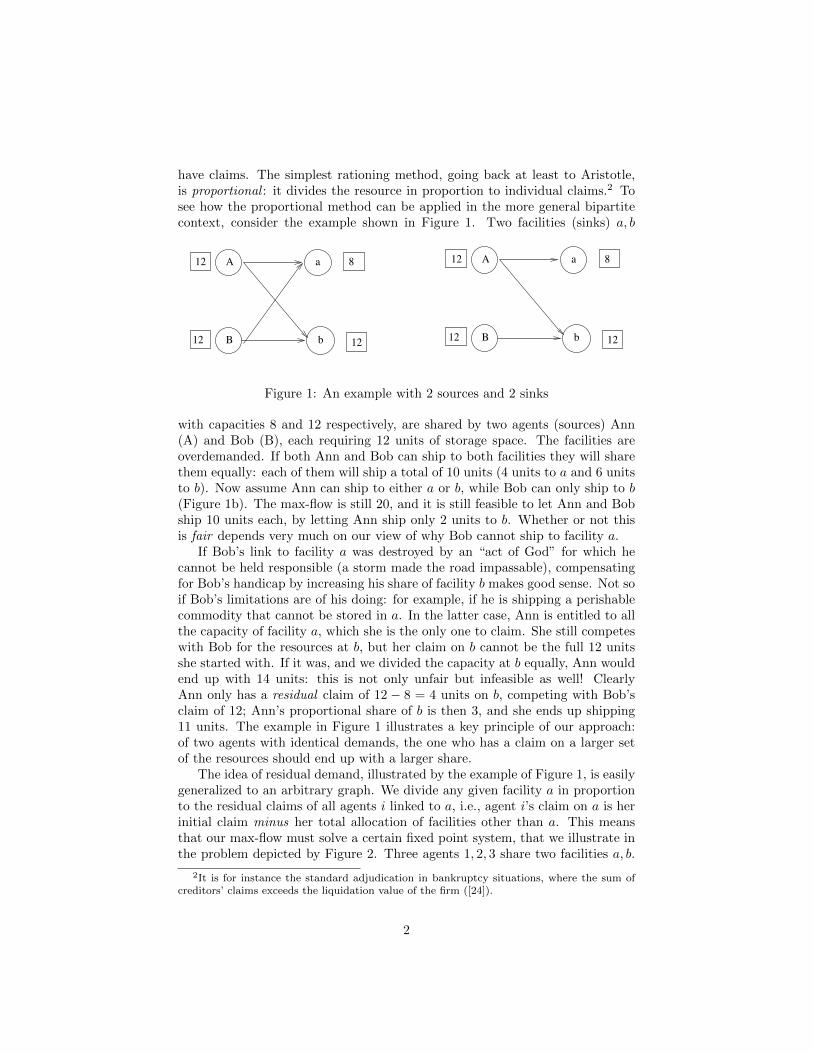
have claims. The simplest rationing method, going back at least to Aristotle,is proportional : it divides the resource in proportion to individual claims.2 Tosee how the proportional method can be applied in the more general bipartitecontext, consider the example shown in Figure 1. Two facilities (sinks) a, b

a

b

12

12

8

12

A

B

a

b

12

12

8

12

A

B

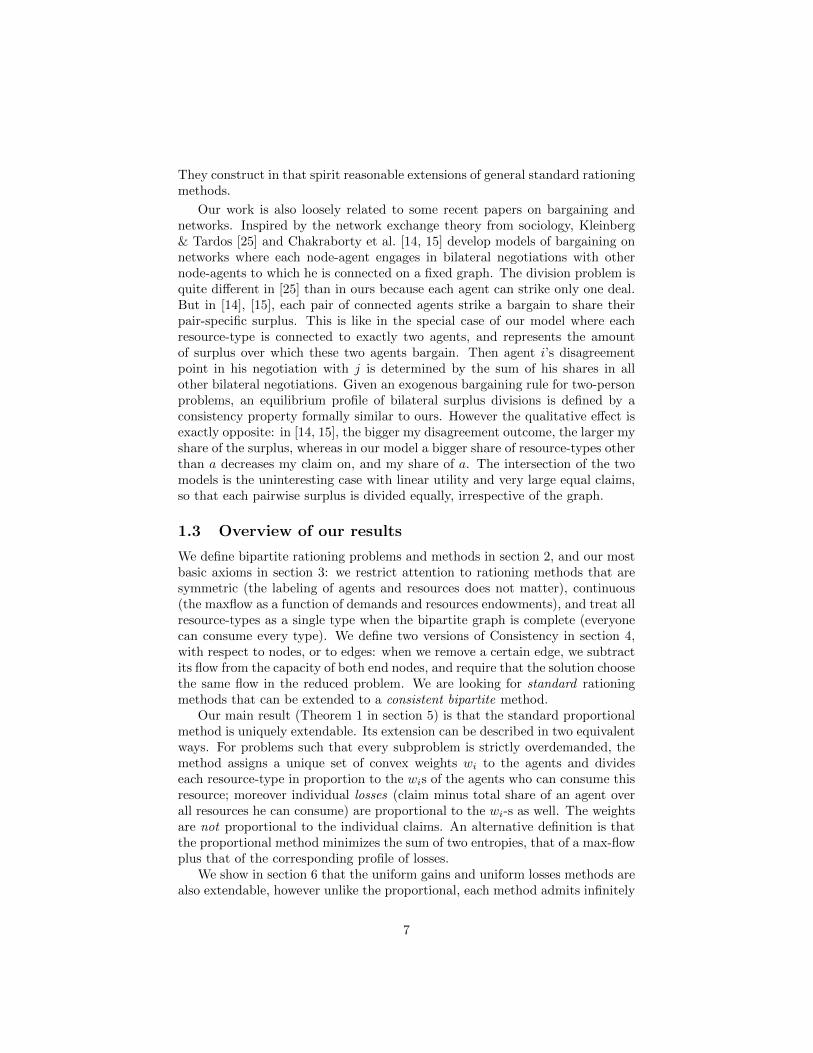
Figure 1: An example with 2 sources and 2 sinks

with capacities 8 and 12 respectively, are shared by two agents (sources) Ann(A) and Bob (B), each requiring 12 units of storage space. The facilities areoverdemanded. If both Ann and Bob can ship to both facilities they will sharethem equally: each of them will ship a total of 10 units (4 units to a and 6 unitsto b). Now assume Ann can ship to either a or b, while Bob can only ship to b(Figure 1b). The max-flow is still 20, and it is still feasible to let Ann and Bobship 10 units each, by letting Ann ship only 2 units to b. Whether or not thisis fair depends very much on our view of why Bob cannot ship to facility a.

If Bob’s link to facility a was destroyed by an “act of God” for which hecannot be held responsible (a storm made the road impassable), compensatingfor Bob’s handicap by increasing his share of facility b makes good sense. Not soif Bob’s limitations are of his doing: for example, if he is shipping a perishablecommodity that cannot be stored in a. In the latter case, Ann is entitled to allthe capacity of facility a, which she is the only one to claim. She still competeswith Bob for the resources at b, but her claim on b cannot be the full 12 unitsshe started with. If it was, and we divided the capacity at b equally, Ann wouldend up with 14 units: this is not only unfair but infeasible as well! ClearlyAnn only has a residual claim of 12 − 8 = 4 units on b, competing with Bob’sclaim of 12; Ann’s proportional share of b is then 3, and she ends up shipping11 units. The example in Figure 1 illustrates a key principle of our approach:of two agents with identical demands, the one who has a claim on a larger setof the resources should end up with a larger share.

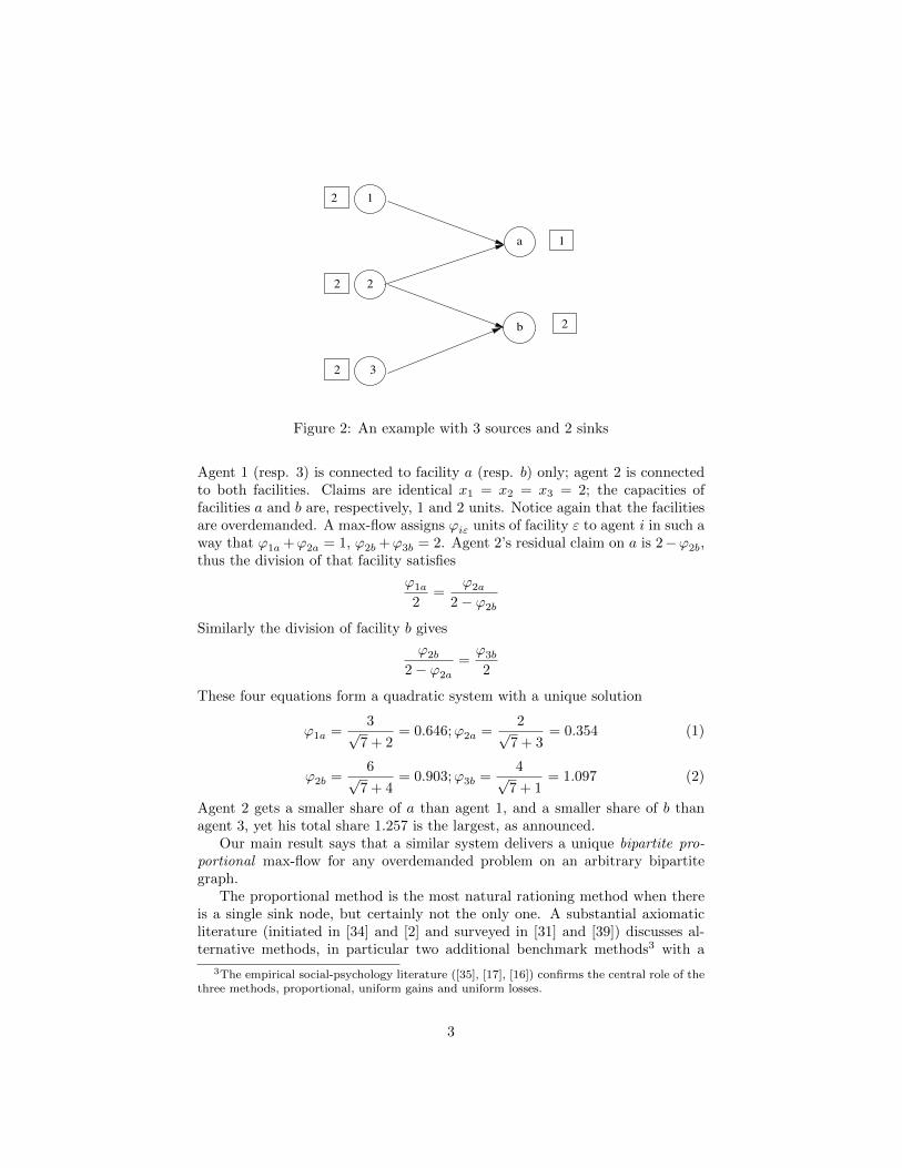
The idea of residual demand, illustrated by the example of Figure 1, is easilygeneralized to an arbitrary graph. We divide any given facility a in proportionto the residual claims of all agents i linked to a, i.e., agent i’s claim on a is herinitial claim minus her total allocation of facilities other than a. This meansthat our max-flow must solve a certain fixed point system, that we illustrate inthe problem depicted by Figure 2. Three agents 1, 2, 3 share two facilities a, b.

2It is for instance the standard adjudication in bankruptcy situations, where the sum ofcreditors’ claims exceeds the liquidation value of the firm ([24]).

2

2

3

a

b

12

2

2

1

2

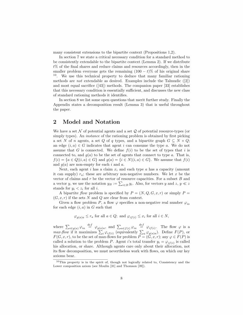
Figure 2: An example with 3 sources and 2 sinks

Agent 1 (resp. 3) is connected to facility a (resp. b) only; agent 2 is connectedto both facilities. Claims are identical x1 = x2 = x3 = 2; the capacities offacilities a and b are, respectively, 1 and 2 units. Notice again that the facilitiesare overdemanded. A max-flow assigns ϕiε units of facility ε to agent i in such away that ϕ1a +ϕ2a = 1, ϕ2b +ϕ3b = 2. Agent 2’s residual claim on a is 2−ϕ2b,thus the division of that facility satisfies

ϕ1a

2=

ϕ2a

2− ϕ2b

Similarly the division of facility b gives

ϕ2b

2− ϕ2a

=ϕ3b

2

These four equations form a quadratic system with a unique solution

ϕ1a =3√

7 + 2= 0.646;ϕ2a =

2√7 + 3

= 0.354 (1)

ϕ2b =6√

7 + 4= 0.903;ϕ3b =

4√7 + 1

= 1.097 (2)

Agent 2 gets a smaller share of a than agent 1, and a smaller share of b thanagent 3, yet his total share 1.257 is the largest, as announced.

Our main result says that a similar system delivers a unique bipartite pro-portional max-flow for any overdemanded problem on an arbitrary bipartitegraph.

The proportional method is the most natural rationing method when thereis a single sink node, but certainly not the only one. A substantial axiomaticliterature (initiated in [34] and [2] and surveyed in [31] and [39]) discusses al-ternative methods, in particular two additional benchmark methods3 with a

3The empirical social-psychology literature ([35], [17], [16]) confirms the central role of thethree methods, proportional, uniform gains and uniform losses.

3

simple interpretation. To describe these methods, it is convenient to think ofeach source node as an agent, and its capacity as that agent’s claim. Similarly,we can think of the sink node as a resource, and its capacity as the amountavailable to be allocated to the agents. The uniform gains method equalizesindividual shares as much as possible provided no one’s share exceeds his claim;the uniform losses method equalizes individual losses under the constraint thatshares are non negative. In addition, a variety of methods provide flexible com-promises between the three benchmarks: a good example is the family of equalsacrifice methods ([42], see section 7 below). We speak of a standard rationingmethod when there is a single sink node, and of a bipartite method in the caseof multiple sink nodes.

The property known as consistency plays a central role in the axiomaticliterature on standard rationing methods4. A method is consistent if, when wetake away one agent from the set of participants, and subtract his share fromthe available resource, the division among the remaining set of claimants doesnot change. It is satisfied by the three benchmark methods, the family of equalsacrifice methods, and many more.

In bipartite rationing problems, we think of each sink node as a different“type” of resource, and the types of resource an agent can consume are perfectsubstitutes to satisfy his total demand. Now we can take away either a sourcenode or a sink node, allowing us to generalize consistency to this more complexmodel. When we take away one agent, we subtract from each resource-type theshare previously assigned to the departing agent; if we remove a resource-type,we subtract from the claim of each agent the share of the departing resource-type he was previously receiving; in each case we insist that the division in thereduced problem remain as before. The argument about residual claims in theexamples of Figure 1 (resp. Fig. 2) is the instance of consistency applied to theremoval of the resource-type a (resp. a then b).

We show how the other two benchmark methods—uniform gains and uniformlosses—can be extended consistently to the bipartite context. Further, we showthat many familiar consistent standard methods cannot be consistently extendedto the bipartite context.

1.1 Interpreting Consistency

The interpretation of the connectivity constraints is critical to our model, andin particular to the Consistency axiom. Consider the substantial literature onmaximum flow problems (see Ahuja et al. [1]) where the goal is to not onlymaximize the quantity distributed, but also to ensure that the distribution isequitable, which is the key motivation behind our model as well.

A typical example is the early contribution of Megiddo [28] who considersa network (not necessarily bipartite) with multiple sources and sinks and as-sumes that the manager wants “not only to maximize the total flow but also

4Variants of this axiom have emerged in a variety of contexts, including TU games, match-ing, assignment, etc., as a compelling rationality property for fair division (see e.g., [27] and[40]). In the words of Balinski and Young:“every part of a fair division should be fair” [3].

4

to distribute it fairly among the sinks or the sources” (p.97). With the ob-jective to “maximize the minimum amount delivered from individual sources”(ibid.), he proves the existence of a lexicographically optimal flow: among allflows maximizing the above minimum amount, it maximizes the second smallestamount delivered, etc5. Brown [10] discusses similarly the equitable distribu-tion of coal during a prolonged coal strike in which only the 20-30% of “non-union” mines were active: the question is to distribute equitably the limited coalsupply amongst the power companies with varying demands and connectivityconstraints.6

Megiddo’s lex-optimal solution aims at equalizing flows going through thevarious sources and sinks, as much as permitted by the connectivity constraints:in the examples of Figure 1b and Fig. 2 where full equality of individual sharesis possible, these constraints have no effect on final shares; e.g., in Figure 1bBob is not penalized for having fewer connections than Ann.

We use the opposite normative postulate that agents should be held respon-sible for their connections.7 In standard rationing models individual demandsrepresent legal rights on the assets of a bankrupt firm ([34, 24]), or on the estateof a deceased person ([34, 2]), fiscal liability toward a levy ([43]), or any sort ofobjective “claim or liability” toward the resources. We generalize the standardmodel in that each individual claim applies to a subset of the resources, butwe still require that the division of each resource-type be fair: the Consistencyproperty achieves this by applying the same standard rationing method (forinstance proportional) to each resource, and allowing each agent with a claimon this particular resource to apply her full residual claim, i.e., her initial claimminus her shares of other resources. This implies for instance that of two agentswith identical claims, the one with richer connections carries a bigger total flow.

The connection-neutral view point a la Megiddo is entirely natural for ap-plications such as famine relief, rationing of coal during a strike, rationing ofblood of types O,A,B, or AB, among patients with these same types. An exam-ple where our connection-responsible viewpoint is compelling is the division ofearmarked funds (as in [8]). Agents compete for the funds of several sponsors(federal agencies, private foundations, etc.); each agent submits a project witha total price tag, and each sponsor attaches some strings to the projects it willconsider (e.g., must have an environmental dimension, must involve minorities,etc.); each project is submitted to all the sponsors of which it meets the con-straints. Here the compatibility of my project with a given source of funds isanything but an act of God. Each sponsor seeks an equitable division of its ownfunds, which a consistent bipartite rationing method provides to all sponsors atthe same time.

5Megiddo later gave an efficient algorithm to find a lex-optimal flow [29]; see also the workof Gallo, Grigoriadis, and Tarjan [21] for a more efficient implementation.

6It is not cost-effective (or feasible) to ship coal from certain mines to certain power plants.7Modern theories of distributive justice (see [36, 19]) emphasize the distinction between

personal characteristics for which individuals should be held responsible, and those for whichthey should not.

5

1.2 Related literature

We already mentioned the lex-optimal approach to fair maximum flows due toMegiddo, Brown, and a substantial extant literature.8 In the same spirit ofconnection-neutrality, Minoux [30] considered a network with a single sourceand a single sink where each arc e cannot carry more than an α(e) fractionof the total flow sent from the source (α(e) is an exogenous parameter); hisgoal is to find a maximum flow that respects these constraints. This modelwas generalized by Zimmermann [44, 45], Hall and Vohra [22], and Betts andBrown [5] to allow for proportional lower and upper bounds on any arc, whereas before the proportional bounds are increasing linear functions of the flowalong one special arc (such as the total flow sent from the source). A typicalapplication of this richer model is aid distribution during famine relief, wherethe proportional lower bounds ensure that no region receives too little of thetotal amount distributed.

Related optimization models such as the linear sharing problem [11] andthe flow-circulation sharing problem [12] all address equitable distribution ofresources in other settings, but again under connection-neutrality.

The work of Bochet et al. [8] is both more recent and closer in spirit toour work. In the same allocation problem with bipartite compatibility con-straints between agents and resource types, they replace the objective claimsof our model by privately held single-peaked preferences over one’s total share,and assume the resources are non disposable. Thus, as in Sprumont’s seminalmodel [38] with a single resource type, distributing all the resources typicallyrequires to give some agents more than their peak allocation, and some less.The connection-neutral extension of Sprumont’s uniform gains method selectsthe Lorenz dominant feasible profile of total shares (it coincides with Megiddo’slex-optimal solution). The corresponding direct revelation mechanism is strat-egyproof 9 (even group-strategyproof: see [13]), a characteristic property underconnection-neutrality.

Bochet et al. [9] is a variant of [8] with strategic agents on both sources andsinks, the source-agents demanding some resource up to some privately heldpeak level, while the sink agents want to supply resource up to their own peaklevel. Efficient trade splits the market in a segment where suppliers get theirpeak allocation while the relevant demanders are rationed, and another segmentwhere the roles are reversed. These authors maintain connection-neutrality andfocus as before on the Lorenz dominant efficient trade.

Random assignment under dichotomous preferences, studied by Bogomol-naia and Moulin [7] and Roth et al. [37], is the special case of [9] where allclaims are for one unit and there is one unit of each resource-type. In thatmodel as here, the assumption of unit claims and unit types does not signifi-cantly simplify the computations.

Finally Ilkilic and Kayi [23] discuss a bipartite rationing model with ob-jective claims and resources like we do here, but under connection neutrality.

8See the survey by Luss [26].9Each agent reports his preferences and the truthful report is a dominant strategy.

6

They construct in that spirit reasonable extensions of general standard rationingmethods.

Our work is also loosely related to some recent papers on bargaining andnetworks. Inspired by the network exchange theory from sociology, Kleinberg& Tardos [25] and Chakraborty et al. [14, 15] develop models of bargaining onnetworks where each node-agent engages in bilateral negotiations with othernode-agents to which he is connected on a fixed graph. The division problem isquite different in [25] than in ours because each agent can strike only one deal.But in [14], [15], each pair of connected agents strike a bargain to share theirpair-specific surplus. This is like in the special case of our model where eachresource-type is connected to exactly two agents, and represents the amountof surplus over which these two agents bargain. Then agent i’s disagreementpoint in his negotiation with j is determined by the sum of his shares in allother bilateral negotiations. Given an exogenous bargaining rule for two-personproblems, an equilibrium profile of bilateral surplus divisions is defined by aconsistency property formally similar to ours. However the qualitative effect isexactly opposite: in [14, 15], the bigger my disagreement outcome, the larger myshare of the surplus, whereas in our model a bigger share of resource-types otherthan a decreases my claim on, and my share of a. The intersection of the twomodels is the uninteresting case with linear utility and very large equal claims,so that each pairwise surplus is divided equally, irrespective of the graph.

1.3 Overview of our results

We define bipartite rationing problems and methods in section 2, and our mostbasic axioms in section 3: we restrict attention to rationing methods that aresymmetric (the labeling of agents and resources does not matter), continuous(the maxflow as a function of demands and resources endowments), and treat allresource-types as a single type when the bipartite graph is complete (everyonecan consume every type). We define two versions of Consistency in section 4,with respect to nodes, or to edges: when we remove a certain edge, we subtractits flow from the capacity of both end nodes, and require that the solution choosethe same flow in the reduced problem. We are looking for standard rationingmethods that can be extended to a consistent bipartite method.

Our main result (Theorem 1 in section 5) is that the standard proportionalmethod is uniquely extendable. Its extension can be described in two equivalentways. For problems such that every subproblem is strictly overdemanded, themethod assigns a unique set of convex weights wi to the agents and divideseach resource-type in proportion to the wis of the agents who can consume thisresource; moreover individual losses (claim minus total share of an agent overall resources he can consume) are proportional to the wi-s as well. The weightsare not proportional to the individual claims. An alternative definition is thatthe proportional method minimizes the sum of two entropies, that of a max-flowplus that of the corresponding profile of losses.

We show in section 6 that the uniform gains and uniform losses methods arealso extendable, however unlike the proportional, each method admits infinitely

7

many consistent extensions to the bipartite context (Propositions 1,2).In section 7 we state a critical necessary condition for a standard method to

be consistently extendable to the bipartite context (Lemma 2). If we distributet% of the final shares and reduce claims and resources accordingly, then in thesmaller problem everyone gets the remaining (100 − t)% of his original share10. We use this technical property to deduce that many familiar rationingmethods are not extendable as desired. Examples include the Talmudic ([2])and most equal sacrifice ([43]) methods. The companion paper [33] establishesthat this necessary condition is essentially sufficient, and discusses the new classof standard rationing methods it identifies.

In section 8 we list some open questions that merit further study. Finally theAppendix states a decomposition result (Lemma 3) that is useful throughoutthe paper.

2 Model and Notation

We have a set N of potential agents and a set Q of potential resource-types (orsimply types). An instance of the rationing problem is obtained by first pickinga set N of n agents, a set Q of q types, and a bipartite graph G ⊆ N × Q;an edge (i, a) ∈ G indicates that agent i can consume the type a. We do notassume that G is connected. We define f(i) to be the set of types that i isconnected to, and g(a) to be the set of agents that connect to type a. That is,f(i) = {a ∈ Q|(i, a) ∈ G} and g(a) = {i ∈ N |(i, a) ∈ G}. We assume that f(i)and g(a) are non-empty for each i and a.

Next, each agent i has a claim xi and each type a has a capacity (amountit can supply) ra; these are arbitrary non-negative numbers. We let x be thevector of claims and r be the vector of resource capacities. For a subset B anda vector y, we use the notation yB :=

∑i∈B yi. Also, for vectors y and z, y � z

stands for yi < zi for all i.A bipartite flow problem is specified by P = (N,Q,G, x, r) or simply P =

(G, x, r) if the sets N and Q are clear from context.Given a flow problem P , a flow ϕ specifies a non-negative real number ϕia

for each edge (i, a) in G such that

ϕg(a)a ≤ ra for all a ∈ Q; and ϕif(i) ≤ xi for all i ∈ N,

where∑i∈g(a) ϕia

def= ϕg(a)a, and

∑a∈f(i) ϕia

def= ϕif(i). The flow ϕ is a

max-flow if it maximizes∑i ϕif(i) (equivalently

∑a ϕg(a)a). Define F (P ), or

F (G, x, r), to be the set of max-flows for problem P = (G, x, r); any ϕ ∈ F (P ) iscalled a solution to the problem P . Agent i’s total transfer yi = ϕif(i) is calledhis allocation, or share. Although agents care only about their allocation, notits flow decomposition, we must nevertheless work with flows, on which our keyaxioms bear.

10This property is in the spirit of, though not logically related to, Consistency and theLower composition axiom (see Moulin [31] and Thomson [39]).

8

We now make a simple observation that lets us assume additional structureon any flow problem without loss of generality. A familiar consequence of themax-flow min-cut theorem ([1]) is that we can decompose any max-flow problemin (at most) two simpler subproblems that can be treated separately. In onesubproblem the sink nodes are overdemanded, in the sense that in every solutionϕ, these resource-types are fully allocated to the underdemanded agents, each ofwhom receives at most his claim; so these agents are rationed. The situation isreversed in the other subproblem, where, in every solution ϕ, the overdemandedagents receive exactly their claim from the underdemanded sink nodes. Becausethere is no edge between two underdemanded nodes, this decomposition cutsour fair division problem in half: we need only to propose a rule for problemswhere the sinks are overdemanded and the sources rationed, then exchange therole of sources and sinks to apply the same rule to problems with overdemandedsources and rationed sinks.

In the rest of the paper, we shall be concerned only with problems in whichthe resources are overdemanded. It is well known (see [1] or [9]) that the sys-tem of inequalities (3), shown below, characterizes the existence of a flow ϕexhausting all resources and transferring at most his claim to each agent i.

Definition 1 A bipartite rationing problem is a flow problem P = (N,Q,G, x, r)such that the resources are overdemanded, namely:

for all B ⊆ Q: rB ≤ xg(B). (3)

Let P denote the set of bipartite rationing problems P = (G, x, r).

Three subsets of P play an important role below. A problem P ∈ P isstrictly overdemanded if

for all B ⊆ Q: rB < xg(B).

Let Pstr be the set of strictly overdemanded problems. A problem P ∈ P isirreducible if every subproblem is strictly overdemanded:

rQ ≤ xN ; for all B Q: rB < xg(B).

Let Pir be the set of irreducible problems.Finally, a P ∈ P is balanced if rQ = xg(Q).Note that a problem P ∈ P�P ir must contain a balanced subproblem, and

so can be further decomposed: focusing on the balanced subproblem, observethat the resources involved are enough to satisfy every agent involved in thebalanced subproblem, so such agents receive nothing from the resources outsideof the subproblem. By iteratively eliminating such balanced subproblems, weend up with at most one irreducible problem. This is the key to the canonicaldecomposition of an arbitrary problem in P into a union of irreducible problems,all but at most one of them balanced: see Lemma 3 in the Appendix.

Note further that an irreducible and balanced problem must have a con-nected graph, however a strictly overdemanded problem need not be connected.

9

Definition 2 A bipartite rationing method (or simply method) H associatesto each problem P ∈ P, where N ⊂ N , Q ⊂ Q, a max-flow ϕ = H(P ) ∈ F(P ).

Note that any agent with zero claim, and any type with zero resource getsno flow in any method.

Definition 3 A rationing problem is standard if it involves a single resourcetype to which all agents are connected. It is a triple P 0 = (N, x, t), wherex ∈ RN+ is the profile of claims, t units of the resource are available, and t ≤ xN .We write P0 for the set of standard problems.

A standard rationing method h is a method applying only to standard prob-lems. Thus h(N, x, t) ∈ RN+ is a division of t among the agents in N such thathi(N, x, t) ≤ xi for all i ∈ N .

We recall the definition of the three benchmark standard rationing methods,proportional hpro, uniform gains hug, uniform losses hul:

hpro(x, t) =xixN· t;

hugi (x, t) = min{xi, λ} where λ solves∑i∈N

min{xi, λ} = t;

huli (x, t) = max{xi − µ, 0} where µ solves∑i∈N

max{xi − µ, 0} = t.

For each resource a ∈ Q, a method H defines a standard rationing method ahby the way it deals with this single resource and the complete graphG = N×{a}:

ah(N, x, ra) = H(N × {a}, x, ra)

3 Basic axioms

As discussed in the introduction, our goal is to understand which standardmethods can be extended to bipartite methods, while respecting a consistencyproperty. As in most of the literature on standard methods (see e.g., [31], [39]),we restrict attention to symmetric and continuous rationing methods.

Symmetry (SYM). A method H is symmetric if the labels of the agentsand types do not matter. Formally, given a permutation π of the agents and apermutation σ of the types, define Gπ,σ to be the graph such that (π(i), σ(a)) ∈Gπ,σ if and only if (i, a) ∈ G. The claims xπ of the agents and resources rπ of thetypes are similarly defined. Suppose H(G, x, r) = ϕ and H(Gπ,σ, xπ, rσ) = ϕ′.Then the method H is symmetric if and only if ϕia = ϕ′π(i)σ(a) for all (i, a) ∈ G.

The standard method associated with a symmetric H is symmetric as well,thus independent of the choice of the type a and the agents N . In keepingwith the rest of our notation, we write it simply as h(x, t), where x→ h(x, t) issymmetric from Rn+ into itself.

10

Continuity (CONT). A method H is continuous if for all N,Q, and G, the

mapping (x, r)→ H(G, x, r) is continuous in the relevant subset of RN+ × RQ+.

We also insist that our methods do not distinguish a problem without anycompatibility constraints (i.e., the graph G is complete) from the correspondingstandard problem where all types are merged into one.

Reduction of Complete Graphs (RCG). Fix a problem P = (N×Q, x, r) ∈P where the graph G is complete. The symmetric method H, with associ-ated standard method h, satisfies RFG if for all N ⊂ N , Q ⊂ Q, and all(N ×Q, x, r) ∈ P, we have

ϕiQ = h(x, rQ) (4)

i.e., the shares y(P ) obtain by merging all resources into a single type.

Definition 4 We write H0 for the set of symmetric and continuous stan-dard rationing methods, and H for the set of symmetric, continuous bipar-tite methods satisfying Reduction of Complete Graphs. We use the notationH(A,B, · · · ),H0(A,B, · · · ) for the subset of methods in H or H0 satisfying ad-ditional properties A,B, · · · .

4 Consistency

We give two versions of the crucial consistency property, both generalizing con-sistency for standard methods.

We use the following notation. For a given graph G ⊆ N × Q, and subsetsN ′ ⊆ N , Q′ ⊆ Q, the restricted graph of G is G(N ′, Q′) := G∩{N ′×Q′}, againnot necessarily connected, and the restricted problem obtains by also restrictingx to N ′ and r to Q′.

Node Consistency (Node-CSY). Fix an agent i ∈ N and a problem P ∈ P,and define the reduced claims and resources under method H ∈ H after thisagent (and all the edges involving this agent) is removed:

xHj (−i) = xj , for all j 6= i

and for ϕ = H(P ):

rHa (−i) = ra − ϕia for all a ∈ f(i); rHb (−i) = rb, for b 6∈ f(i).

The reduced problem is (G(N∗, Q∗), xH(−i), rH(−i)), where N∗ = N \ {i},and Q∗ = f(N∗). Similarly, fix a type a ∈ Q and define the reduced claimsand resources under method H after this type (and all the edges involving thistype) is removed:

xHj (−a) = xj − ϕja for all j ∈ g(a); xHj (−a) = xj , for j 6∈ g(a).

andrHb (−a) = rb, for all b 6= a

11

The reduced problem is (G(N∗∗, Q∗∗), xH(−a), rH(−a)), where Q∗∗ = Q \ {a},N∗∗ = g(Q∗∗).

Suppose H(G(N,Q), x, r) = ϕ, H(G(N∗, Q∗), xH(−i), rH(−i)) = ϕ′, andH(G(N∗∗, Q∗∗), xH(−a), rH(−a)) = ϕ

′′. The method H ∈ H is node-consistent

if for all N ⊂ N , Q ⊂ Q, all (G, x, r) ∈ P, all i ∈ N , a ∈ Q: ϕjb = ϕ′jb for all

jb ∈ G(N∗, Q∗) and ϕjb = ϕ′′

jb for all jb ∈ G(N∗∗, Q∗∗).

Edge Consistency (Edge-CSY). Edge-consistency is stronger than node-consistency. Fix an edge ia ∈ G and define the reduced claims and resourcesunder method H after this edge is removed:

xHi (−ia) = xi − ϕia; xHj (−ia) = xj for j 6= i

rHa (−ia) = ra − ϕia; rHb (−ia) = rb for b 6= a

The corresponding reduced problem is (G�{ia}, xH(−ia), rH(−ia)), where theset of agents is N∗ = N unless f(i) = {a} in which case N∗ = N�{i}; similarlythe set of types is Q∗ = Q unless g(a) = {i} in which case Q∗ = Q�{a}.

Suppose H(G, x, r) = ϕ and H(G \ {ia}, xH(−ia), rH(−ia)) = ϕ′. Themethod H ∈ H is edge-consistent if for all N ⊂ N , Q ⊂ Q, all (G, x, r) ∈ P,and ia ∈ G: ϕjb = ϕ′jb for all jb ∈ G�{ia}.

Clearly, for either one of the three reductions just discussed, the reducedproblem is overdemanded if the initial problem is, but not necessarily strictlyoverdemanded or irreducible if the initial problem is. Note also that G�{ia}may not be connected even if G is connected.

5 The bipartite proportional method

Given the prominent role of the standard proportional method in H0, the firstquestion is to look for a bipartite extension. It turns out that there is a uniquesuch extension Hpro satisfying Node-CSY.

Theorem 1 gives two equivalent definitions of this method, one for anyoverdemanded problem as the solution of a maximization problem, the otherfor irreducible problems only. The latter definition is then extended to anyoverdemanded problem by means of its canonical decomposition in irreduciblesubproblems (Definition 5 in the Appendix). The latter definition gives muchmore insight into the structure of our method.

We use two new pieces of notation. The unit simplex of RN is written below

as S(N), and its interior as◦S(N) = {w|wN = 1 and wi > 0 for all i}. For

any z ≥ 0, we define the function En(z) = z ln(z), with the convention thatEn(0) = 0. Note that the sum

∑k En(zk) is the familiar entropy of a vector z.

Note also that En(z) is strictly convex.For any problem P = (G, x, r) ∈ P, define ϕ(P ) as

ϕ(P ) = arg minϕ∈F(G,x,r)

∑ia∈G

En(ϕia) +∑i∈N

En(xi − φif(i)) (5)

12

Problem (5) has a unique solution ϕ for any P ∈ P because the objectivefunction is strictly convex and finite. This defines the proportional method,Hpro, which associates with each problem P the solution ϕ(P ), that we call theproportional flow for P .

The following result establishes additional properties of the proportionalmethod and provides an alternative definition of the proportional flow.

Theorem 1i) The proportional method Hpro is in H and is edge-consistent: Hpro ∈H(Edge− CSY ).ii) For any irreducible problem P = (G, x, r) ∈ P ir, the following system withunknown w ∈ S(N)

xi = wi · (xN − rQ) +∑a∈f(i)

wiwg(a)

ra for all i ∈ N (6)

has a unique solution w in◦S(N), and the proportional flow is

ϕia =wiwg(a)

ra (7)

iii) The method Hpro is the only continuous and node-consistent method thatis proportional for standard problems.

For instance the example of Figure 2 is irreducible, and the system (7) writes

ϕia =wi

w1 + w2· 1 for i = 1, 2; ϕib =

wiw2 + w3

· 2 for i = 2, 3

Moreover (6) gives xi − yi = wi · (xN − rQ), i.e.,

2− ϕ1a

w1=

2− (ϕ2a + ϕ2b)

w2=

2− ϕ3b

w3= 3

The unique solution

w1 =1

3(4−

√7);w2 =

1

9(5√

7− 11);w3 =2

9(4−

√7)

confirms the flow (1), (2) found in section 1.

Equation (7) explains our proportional terminology for the method Hpro.Indeed the flow ϕ distributes each resource a proportionally between the agentsconnected to a, however the proportionality is not with respect to the originalclaims, but with respect to the “adjusted claims” w. The adjustments accountfor the asymmetry in the connections of the various agents. The relationshipbetween the adjusted claims and the original claims is given in Equation (6).

Proof of Theorem 1We first argue that Hpro is symmetric and continuous. It is clear that any

relabeling of the agents and resources does not change the optimization problem

13

characterizing the proportional solution, so symmetry follows immediately. Thefact that Hpro is continuous follows from Berge’s Maximum Theorem ([6]): Theobjective function is continuous, and the correspondence (x, r) → F(G, x, r)is compact-valued, and continuous as well (upper and lower hemicontinuous);therefore the argmin correspondence is continuous as well.

We observe immediately after this proof thatHpro satisfies a property strongerthan RCG, dubbed Merging of Identical Resource-types, so a direct proof ofRCG is not needed at this point.Step 1: Statement i) For Edge-CSY, we fix P = (G, x, r) and an edge ia ∈ G.For any ϕ′ ∈ F(G\{ia}, xH(−ia), rH(−ia)), adding ia to G and ϕia to ϕ′ yieldsa flow (ϕ′, ϕia) in F(G, x, r). The objective function at (ϕ′, ϕia) is the same asat ϕ′ plus the single term En(ϕia), because xi − yi = xHi (−ia) − yHi (−ia).Thus if the restriction of ϕ to PH(−ia) is not optimal in that problem, we canconstruct a flow (ϕ′, ϕia) beating ϕ in P .

Step 2: Statement ii) We fix an irreducible problem P = (G, x, r). It will beconvenient to replace problem (5) by the equivalent problem

minϕ∈F(G,x,r)

∑ia∈G

Ln(ϕia) +∑i∈N

Ln(xi − ϕif(i)) (8)

where Ln(z) = z(ln(z)− 1) is still strictly convex and has derivative ln(z). Theequivalence follows from the fact that we are subtracting two constant terms tothe objective function:

∑ia∈G ϕia = rQ and

∑i∈N (xi − ϕif(i)) = xN − rQ.

Step 2.1 We assume in this sub-step xN = rQ: P is balanced. By irreducibil-ity, for every (i, a) ∈ G, there is a solution ϕ ∈ F(G, x, r) with ϕia > 0. Also,because the problem is balanced, ϕif(i) = xi for every ϕ ∈ F(G, x, r). ThusProblem (8) becomes

minϕ∈F(G,x,r)

∑ia∈G

Ln(ϕia),

whose Lagrangean is given by

L(ϕ, λ, µ) =∑

(i,a)∈G

ϕia[ln(ϕia)−1]+∑i∈N

λi(xi−∑a∈Q

ϕia)+∑a∈Q

µa(ra−∑i∈N

ϕia),

where λ = (λi)i∈N ∈ RN+ and µ = (µa)a∈Q ∈ RQ. Define

q(λ, µ) = minϕ≥0

L(ϕ, λ, µ). (9)

It is easy to check that for any fixed λ and µ, the minimum is attained in (9)uniquely by the solution ϕ∗ia = eλi+µa , using which we get

q(λ, µ) = L(ϕ∗, λ, µ) = −∑

(i,a)∈G

ϕ∗ia +∑i∈N

λixi +∑a∈Q

µara.

The associated dual problem is thus given by

maxλ,µ

{−

∑(i,a)∈G

eλi+µa +∑i∈N

λixi +∑a∈Q

µara

}. (10)

14

It is clear that (10) has a unique optimal solution that is given by the solutionto the following system of equations:

−∑a∈f(i)

eλi+µa + xi = 0, ∀i ∈ N,

and−∑i∈g(a)

eλi+µa + ra = 0, ∀a ∈ Q.

Letting λ∗ and µ∗ be the optimal solutions, we have

eλ∗i =

xi∑a∈f(i) e

µ∗a; eµ

∗a =

ra∑i∈g(a) e

λ∗i.

Finally,ϕ∗ia = eλ

∗i eµ

∗a .

In particular, taking wi = eλ∗i∑

N eλ∗j

verifies (6) and (7).

Step 2.2 We assume now that P = (G, x, r) is not only irreducible, but alsostrictly overdemanded, i.e. xN > rQ. We proceed as before by writing theLagrangean of Problem (8), which is now

L(ϕ, λ, µ) =∑

(i,a)∈G

Ln(ϕia) +∑i∈N

Ln

(xi −

∑a∈f(i)

ϕia

)+∑i∈N

λi(xi −∑a∈Q

ϕia) +∑a∈Q

µa(ra −∑i∈N

ϕia).

As before, for any fixed λ and µ, the minimum in the problem

q(λ, µ) = minϕ≥0

L(ϕ, λ, µ)

is attained uniquely by the solution of

ϕ∗iaxi −

∑a∈f(i) ϕ

∗ia

= eλi+µa .

An implication of this is that in the minimizer of q(λ, µ), each agent’s allocationyi is such that yi < xi. This implies that the optimal choice of λ in the associateddual problem maxλ≥0,µ q(λ, µ) is λ∗ = 0. Also, it is straightforward to check thatthe dual is a maximization problem with a strictly concave objective function,and so has a unique optimal solution µ∗. Using this, the optimal ϕ∗ia satisfy(xi−

∑b:b∈f(i) ϕ

∗ib)e

µ∗a = ϕ∗ia. Letting y∗i =∑b:b∈f(i) ϕ

∗ib, we see, in particular,

thatϕ∗ia

xi − y∗i=

ϕ∗jaxj − y∗j

=ra

xg(a) − y∗g(a), for all a and i, j ∈ g(a) (11)

15

Setting wi =xi−y∗ixN−rQ , so that w ∈

◦S(N), we see that w is a solution of system

(6). Moreover (11) implies (7) as well.

Step 3: Statement iii)Let H be a continuous and node consistent method, proportional for stan-

dard problems. Pick first a strictly overdemanded P = (G, x, r) ∈ Pstr. Fix atype a and reduce P by dropping successively all nodes but a. Then Node-CSYand the fact that H is proportional for one-type problems imply:

for all i ∈ g(a) : ϕia = hpro(x− y + ϕ·a, ra) =xi − yi + ϕia

xg(a) − yg(a) + rara; or ϕia = 0

(12)If yi = xi this implies either ϕia = 0 or {ϕia = ra and {yj = xj and ϕja = 0for all j ∈ g(a)}}. Restricting attention to a connected component of G, thisimplies that every resource goes to a single agent and they all have yj = xj ,contradiction.

So yi < xi for all i. Then (12) implies ϕia > 0 for all ia ∈ G. It also reducesto

ϕia =xi − yi

xg(a) − yg(a)ra ⇒

ϕiaxi − yi

=ϕja

xj − yj=

raxg(a) − yg(a)

for all i, j ∈ g(a)

These are precisely the KKT optimality conditions, so ϕ = ϕ∗.

Pick next P = (G, x, r) irreducible and balanced. Both H and the proportionalbipartite method Hpro are continuous, and P can be expressed as the limit ofstrictly overdemanded problems 11. Thus H = Hpro on Pir.

Finally, both methods H and Hpro are node-consistent on P, so as explainedafter Definition 6 in the Appendix, they are the canonical extension of theirprojection on Pir, where they coincide.

We note that the proof of statement iii) only requires to assume consistencywith respect to the elimination of resource-types.�

The proportional method, as well as all methods discussed in the next twoPropositions, satisfies a (much) stronger property than Reduction of CompleteGraphs: if two resource-types are compatible with exactly the same set of agents,they need not be treated as separate types in the sense that merging them intoa single type while adding their resources is of no consequence to any agent.Thus the artificial creation of new resource-types does not matter.

Merging Identically Connected Resource-types (MIR). Fix a problemP ∈ P and suppose that in the graph G ⊆ N×Q, two types a1, a2 are such thatg(a1) = g(a2). Let G∗ ⊆ N × (Q�{a1, a2} ∪ {a∗}) be the graph obtained bymerging those two types into a new node labeled a∗ with the same connections.The corresponding merged problem (G∗, x, r∗) has r∗a∗ = ra1 + ra2 , r∗a = ra forall a ∈ Q�{a1, a2}.

11Consider the sequence of problems P ε = (G, xε, r) with xεi = xi+ε for all i, and let ε→ 0.For every ε > 0, P ε is strictly overdemanded.

16

Suppose H(G, x, r) = ϕ and H(G∗, x, r∗) = ϕ∗. The method H ∈ H al-lows the merging of identically connected types if for all N ⊂ N , Q ⊂ Q, all(G, x, r) ∈ P, and a1, a2 s.t. g(a1) = g(a2): ϕ∗ia∗ = ϕia1 + ϕia2 for all i ∈ g(a∗),ϕ∗ja = ϕja for all a ∈ Q�{a1, a2}, ja ∈ G. In particular individual shares yi areunchanged.

To check that Hpro satisfies MIR, we fix an irreducible problem (G, x, r)with weights wi = xi

xNsolving (6), and assume g(a1) = g(a2). After merging a1

and a2 into a, the weights wa = wa1 + wa2 , wb = wb for b 6= a1, a2, satisfy thecorresponding system (6) in the merged problem, so statement i) implies thatMIR holds in Pir. For a general (G, x, r) ∈ P we use its canonical decompositionin irreducible problems (Lemma 3 in the Appendix): clearly two nodes such thatg(a1) = g(a2) must be in the same component Qk of the decomposition, whereMIR applies, and the merging of these two nodes reduce Qk by one type andpreserves the rest of the decomposition.

We can formulate an axiom parallel to MIR for the merging of agents. Whentwo agents i, j have identical connections, f(i) = f(j), we can merge them intoa single agent, and endow this superagent with the sum of their claims. Thecorresponding “merging of identically connected agents” (MIA) property saysthat the flow in all edges not involving i or j must be unchanged, while the flowin the merged edges is the sum of the two earlier flows.

This property is known to force the proportional method for standard prob-lems ([4], [32]), and in the bipartite context it takes us uniquely to its canonicalextension: system (6) implies at once that Hpro satisfies MIA. This yields analternative characterization of the bipartite proportional method, by continuity,node (resource-types) consistency, and merging of identically connected agents.

The critical difference between MIR and MIA is that the latter applies exclu-sively to the bipartite proportional method, whereas the former holds true formany more consistent bipartite methods, such as all the extensions of uniformgains and uniform losses in the next section, and all loss calibrated methodsdiscussed in [33].

We conclude this section with one more agreeable feature of Hpro: if agentsi, j have identical claims but i is better connected, she gets a weakly biggershare than j. This is illustrated by the examples in Figures 1,2 (section 1), itcorresponds to the following property:

Monotonicity in Connections (MC). A method H ∈ H is monotonic inconnections if for all (N,Q,G, x, r) and all i, j ∈ N : {xi = xj and f(i) ⊇f(j)} ⇒ yi ≥ yj.

Fix (G, x, r) and i, j as in the premises of MC with xi = xj = z. Letϕ = Hpro(G, x, r). Delete all resource-types except those in f(j), and all agentsexcept i, j. The reduced problem has the complete graph {i, j} × f(j), andclaims x′i = z − ϕiQ�f(j), x

′j = z. Set δ = ϕiQ�f(j) and t to be the total

resource available in the reduced problem. Note t ≤ 2z−δ. Consistency implies

yj =z

2z − δt; yi =

z − δ2z − δ

t+ δ ⇒ yi ≥ yj

17

6 Extensions of uniform gains and uniform losses

A straightforward generalization of Problem (5) delivers a large family of edge-consistent bipartite methods.

Lemma 1 Fix a strictly convex function W and a convex function B, bothfrom R into itself. For any problem (N,Q,G, x, r) ∈ P the flow

ϕ = arg minϕ∈F(G,x,r)

∑ia∈G

W (ϕia) +∑i∈N

B(xi − ϕif(i)) (13)

defines an edge-consistent, symmetric, and continuous bipartite rationing method.We explain in the next section that the typical method H defined by (13)

does not meet RCG (see the Corollary to Lemma 2).Proof . The flow ϕ is well defined because the objective function is strictly

convex and finite. For Symmetry and Continuity we repeat the correspondingargument in the proof of Theorem 1. For Edge-CSY we fix (G, x, r), an edgeia ∈ G, and let ϕ be given by (13). With the notation in the definition of Edge-CSY, observe that if ϕ′ ∈ F(G \ {ia}, x(−ia), r(−ia)), then adding ia to G andϕia to ϕ′ yields a flow (ϕ′, ϕia) in F(G, x, r). If the restriction of ϕ to P (−ia) isnot optimal in that problem, we can then construct a flow (ϕ′, ϕia) beating ϕ inP . In the reduced problem (G�{ia}, x(−ia), r(−ia)) the restriction ϕ−iaof ϕto G�{ia} is clearly a max-flow and x(−ia)− ϕ−iaif(i)�{a} = xi−ϕif(i), implyingEdge-CSY.�

The bipartite proportional method corresponds to W = B = En, and weknow from Theorem 1, this is the only edge-consistent extension of the standardproportional method. By contrast, the bipartite rationing methods in Lemma1 contain infinitely many extensions of uniform gains, and, in a limit sense, ofuniform losses as well.

6.1 Extending uniform gains

It is well known (see De Frutos and Masso [20]) that for any (x, t) ∈ P0, andfor any W strictly convex, we have hug(x, t) = arg miny≤x,yN=t

∑i∈N W (yi).

Therefore setting B ≡ 0 in (13) delivers a consistent bipartite extension HW ofhug, satisfying Merging of Identically Connected Resource-types.

Proposition 1 For any strictly convex function W from R+ into itself, andany problem (N,Q,G, x, r) ∈ P , the flow

◦ϕ = arg min

ϕ∈F(G,x,r)

∑ia∈G

W (ϕia) (14)

defines a method HW in H(Edge−CSY,MIR) satisfying Merging of IdenticallyConnected Resource-types, and extending the standard method hug. Differentchoices of W yield infinitely many different methods HW .

Proof We fix (G, x, r) and describe the Kuhn Tucker conditions character-

izing◦ϕ in (14) with associated net shares yi =

◦ϕif(i). If yi < xi for some agent i,

18

then we must have◦ϕia ≥

◦ϕja for all a ∈ f(i) and j ∈ g(a): otherwise a transfer

from◦ϕja to

◦ϕia yields a better flow. Thus the KKT conditions: for all i, j and

a ∈ f(i) ∩ f(j)

yi < xi ⇒◦ϕia = max

j∈g(a)

◦ϕja for all i, j and a ∈ f(i) ∩ f(j) (15)

Proof of the first statement. By Lemma 1 we need only to check that HW

satisfies MIR (which implies RCG). But it is clear that if in (G, x, r) the types a, bhave g(a) = g(b), and the flow ϕ meets the KKT conditions (15), then mergingthe flows though a and b gives a new flow still meeting the KKT conditions, sowe are done.

Proof of the second statement. If equal split of each resource-type a among

g(a) is feasible (does not exceeds any claim), it will be◦ϕ for any W . When

G is the complete graph, by RCG the profile of net shares is y = hug(x, rQ).However, even in the case G = N × Q, the choice of W will matter because

it may affect the optimal flow◦ϕ. Assume for instance N = {1, 2}, x = (1, 4),

Q = {a, b}, r = (1, 3). Then hug(x, rQ) = (1, 3), and the corresponding max-flows take the form

ϕ1a = z;ϕ1b = 1− z;ϕ2a = 1− z;ϕ2b = 2 + z

for some z ∈ [0, 1]. Choose W 1(z) = −z2, and W 2(z) = ln(z), so thatW 2 guarantees ϕia > 0 for all ia ∈ G whereas W 1 does not. Check thatarg maxz{W 1(z) + 2W 1(1 − z) + W 1(2 + z)} = {0}, that is the single unit oftype a goes to agent 2, who also gets 2 units of type b. On the other hand theoptimal z for W 2 is 1

2 (√

3 − 1), so agent 2 gets 0.63 units of type a and 2.37units of type b.

If G is not complete, even the shares y1, y2 may differ. For an example wemodify our earlier numerical example in Figure 2 by keeping the same graphG, but with claims x = (1, 1, 4) and resources r = (1, 4). For any max-flow wehave ϕ2b < ϕ3b, therefore (15) implies ϕ2a + ϕ2b = 1 for any choice of W . Themax-flows take the form

ϕ1a = z;ϕ2a = 1− z;ϕ2b = z;ϕ3b = 4− z

so for the same functions W 1,W 2 we get z1 = 0 and z2 > 0.It is now clear that (14) defines infinitely many different bipartite methods.�

6.2 Extending uniform losses

The standard uniform losses method obtains ashul(x, t) = arg miny≤x,yN=t

∑i∈N B(xi − yi), for any B strictly convex (see

again [20]). However setting W ≡ 0 in (13) and choosing B strictly convexdoes not define a bipartite rationing method because it does not specify theentire flow ϕ, only the net shares yi = ϕif(i). But a lexicographic minimization,

first of∑i∈N B(xi− yi) delivering the net shares

·y, then of

∑ia∈GW (ϕia) over

19

F(G,·y, r) does the trick. Note that the resulting flow is also the limit of the

solution of (13) for the pair W,µB when the parameter µ goes to infinity.In the following we write the set of feasible net shares at problem (G, x, r) ∈

P as

Y(G, x, r) = {y ∈ RN++|for some ϕ ∈ F(G, x, r) : yi = ϕif(i) for all i}

Proposition 2 Fix any two strictly convex function W,B from R+ intoitself. For any problem (G, x, r) ∈ P, the net shares

·y = arg min

y∈Y(G,x,r)

∑i∈N

B(xi − yi)

and the flow·ϕ = arg min

ϕ∈F(G,·y,r)

∑ia∈G

W (ϕia)

define a method HB�W in H(Edge − CSY,MIR), extending the standardmethod hul. The choice of B does not matter, but different choices of Wyield infinitely many different methods HB�W .

Proof The resulting flow is well defined because B,W are both strictlyconvex, and we already noted that it gives the uniform losses shares when |Q| =1. The method is clearly symmetric, and Continuity follows from applying

Berge’s Maximum Theorem twice, once to (x, r)→ ·y, then to (

·y, r)→ ·

ϕ.For Edge-CSY, we fix (G, x, r) ∈ P and pick ia ∈ G and y′ ∈ Y(G \

{ia}, x(−ia), r(−ia)): the profile y : yi = y′i +·ϕia, yj = y′j for j 6= i, is in

Y(G, x, r). Moreover for any B we have∑j∈N B(xj(−ia)−y′j) =

∑j∈N B(xj−

yj). Therefore the optimal net shares in the reduced problem are y′ : y′i =·yi −

·ϕia, y

′j = yj for j 6= i. Finally the separability of the objective function∑

ia∈GW (ϕia) implies ϕ′e =·ϕe for all e ∈ G�{ia}.

For MIR, fix (G, x, r) and two types a, b such that g(a) = g(b). Merging

the flows though a and b leaves Y(G, x, r) unchanged, hence·y as well; the flow

·ϕ ∈ Y(G,

·y, r) is also merged as desired, by exactly the same argument as in

the proof of Proposition 1.We check next that the choice of B does not matter. This follows from

the observation that we can represent Y(G, x, r) as the core of a submodularcooperative game12 in N , and the familiar fact that such a core has a Lorenzdominant element ([18]). Thus {x}−Y(G, x, r) has a Lorenz dominant elementas well, and a characteristic property of this vector is that for any strictly convexB, it minimizes

∑i∈N B(zi) over {x} − Y(G, x, r).

For the final statement about the infinite number of bipartite extension, werepeat the argument in the proof of Proposition 1.�

12Setting the value of coalition S ⊆ N as v(S) = min∅⊆T⊆S{xT + rf(S�T )}, then y ∈Y(G, x, r)⇔ yS ≤ v(S) for all S, with equality for S = N (see [9]). Then {x} − Y(G, x, r) isthe core of the supermodular game w(S) = xS − v(S).

20

7 Standard methods not consistently extendable

After establishing that the three benchmark methods are extendable toH(Node−CSY ), it is natural to ask whether any consistent standard method h is extend-able as well. The answer is no, because the combination of Node-CSY and RCGimposes the following necessary condition for extendability.

Lemma 2 Assume the set Q of potential resource types is infinite, andpick any bipartite rationing method H ∈ H(Node − CSY ) with correspondingstandard method h ∈ H0. Then for all (N, x, t) ∈ P0 and all δ ∈ [0, 1], we have

h(x− δ · h(x, t), (1− δ)t) = (1− δ) · h(x, t) (16)

Proof Fix (N, x, t) ∈ P0, two integers p, q, 1 ≤ p < q, and a set Q of typeswith cardinality q. Consider the problem P = (N × Q, x, r) where ra = t

q for

all a ∈ Q, with associated profile of shares y at ϕ = H(P ). By RCG y = h(x, t)and by symmetry ϕia = yi

q for all i ∈ N . Drop now p of the nodes and let Q′

be the remaining set of types. Applying Node-CSY p successive times gives

H(N ×Q′, x′, r′) = ϕ′

where x′ = x− pq y, r

′a = t

q for all a ∈ Q′, and ϕ′ is the restriction of ϕ to N×Q′.Therefore y′ = q−p

q y. RCG in the reduced problem gives y′ = h(x′, q−pq t). We

just showed q−pq y = h(x− p

q y,q−pq t), precisely (16) for δ = p

q . Then continuity

implies (16) for other real values of δ.�

Property (16) is a new axiom13 in the theory of standard rationing methods.We distribute first a fraction δ of the shares h(x, t), and decrease accordinglyindividual claims before distributing the remaining (1 − δ)t units of resource:the result is the same as if we distributed all t units in one shot.

It is easy to check directly that our three benchmark standard methods meet(16), which we already know because we showed in the previous sections theyare consistently extendable. On the other hand many (if not most) standardmethods discussed in the literature (see surveys [39],[31]) fail this property. Weillustrate this fact first with two well known examples, the Talmudic method([2]) and the family of equal sacrifice methods ([43], [31]), then with the methodsdefined in Lemma 1.

The Talmudic method hT is a mixture of uniform gains and uniform lossesin the following sense:

hT (x, t) = hug(x

2, t) if t ≤ xN

2; =

x

2+ hul(

x

2, t− xN

2) if

xN2≤ t ≤ xN

An equal sacrifice method is determined by a function u : R+ → R+ ∪ {−∞}with strictly positive derivative. The solution y = hu(x, t) of (N, x, t) ∈ P0 isdefined by budget balance and

for all i: yi > 0⇒ u(xi)− u(yi) = maxN{u(xj)− u(yj)}

13It is reminiscent of the star-shaped invariance axiom in axiomatic bargaining theory: seethe survey [41]. See also the discussion in [33].

21

The proportional method corresponds to u(z) = ln(z), and uniform losses tou(z) = z. Uniform gains is not an equal sacrifice method.

Corollary 1 The Talmudic method, and all equal sacrifice methods, exceptthe proportional and uniform losses, are not extendable to H(Node− CSY ).

Proof. For the Talmudic hT , take n = 2 and check that hT ((4, 2), 3) = (2, 1),while hT ((4, 2)− 1

2 (2, 1), 32 ) = ( 34 ,

34 ) 6= 1

2 (2, 1).Fix now an equal sacrifice method satisfying (16), with corresponding bench-

mark function u. We must show that u is, up to a positive affine transformation,u(z) = ln(z) or u(z) = z. Fix y1, y2, ε1, ε2, all positive, and such that

u(y1 + ε1)− u(y1) = u(y2 + ε2)− u(y2) (17)

Then y = h(x, t) for x = y+ ε and t = y1 + y2. Applying now (16) for δ ∈ [0, 1],we get

u(δ′y1 + ε1)− u(δ′y1) = u(δ′y2 + ε2)− u(δ′y2) (18)

(recall the notation δ′ = 1 − δ). For fixed y, equation (17) defines on somepositive interval [0, α[ a one-to-one function ε1 → ε2 with derivative at zerou′(y2)u′(y1)

. Equation (18) defines the same function for any δ′ ∈ [0, 1], and its

derivative at zero is now u′(δ′y2)u′(δ′y1)

, therefore

u′(y2)

u′(y1)=u′(δ′y2)

u′(δ′y1)for all y1, y2 > 0 and all δ′ ∈ [0, 1] (19)

An affine transformation of u gives the same equal sacrifice method. So we canrescale u so that u′(1) = 1 and take y2 = 1 in (19). We get

u′(ab) = u′(a)u′(b) for all a, b s.t. min{a, b} ≤ 1

This implies u′(a)u′( 1a ) = 1. If min{a, b} > 1 we write u′((ab) 1

b ) = u′(ab)u′( 1b )

and deduce that u′(ab) = u′(a)u′(b) holds for all a, b > 0. This classic functionalequation implies that u′ is a power function, thus after another rescaling, theonly possibilities are u(z) = zp for p > 0, or u(z) = −zp for p < 0, or u(z) =log(z). The latter is the proportional method, for which (16) is true. Dittofor the uniform losses method, corresponding to u(z) = z. But for any othermethod, (16) fails to be true. A simple way to check this is to fix y1 = 2, y2 = 4,choose a, b > 0 such that the power p equal sacrifice method selects y in theproblem x = (a + 2, b + 4), t = 6, and apply (16) for δ = 1

2 . This writes asfollows, for all positive a, b:

{(a+ 2)p − 2p = (b+ 4)p − 4p} ⇒ (a+ 1)p − 1 = (b+ 2)p − 2p

Then one checks that the two curves defined respectively by the left equationand the right equation are distinct if p 6= 0, 1.�

We turn to the Edge-Consistent methods HW,B identified in Lemma 1. Thecorresponding standard method hW,B computes the shares y = hW,B(x, t) asfollows:

y = arg miny≤x,yN=t

∑i∈N

W (yi) +∑i∈N

B(xi − yi) (20)

22

Corollary 2 Assume W,B are both strictly convex. The standard method(20) meets (16) if and only if, up to normalization, W is the entropy functionW ∗(z) = z ln(z).

Proof We give the proof when W,B are both smooth; it extends to generalstrictly convex functions by a straightforward limit argument that we omit forbrevity. We write w, b for the derivatives of W,B.Statement if. Pick any (x, t) ∈ P0 and set y = hEn,B(x, t). From w(0) = −∞follows that yi > 0 for all i s.t. xi > 0, and the KKT conditions characterizingy are

for all i: yi < xi ⇒ ln(yi) + b(xi − yi) = maxj∈N{ln(yj) + b(xj − yj)}

Now for δ ∈]0, 1[ and any i we have yi < xi ⇔ δ′yi < xi− δyi, where we use thenotation δ′ = 1− δ. The above equality can be rewritten as

ln(δ′yi) + b((xi − δyi)− δ′yi) = maxj∈N{ln(δ′yj) + b((xj − δyj)− δ′yj)}

so δ′y meets the KKT conditions for hEn,B(x− δy, δ′t).Statement only if. Because b increases strictly, for any y1, y2, positive and closeenough, there exists z1, z2, positive and such that

w(y1)− b(z1) = w(y2)− b(z2)

Thus the shares y = (y1, y2) are an interior solution of the program (20) forthe problem (z + y, t = y1 + y2), i.e., hW,B(z + y, t) = y. Property (16) giveshW,B(z + δy, δt) = δy for all δ ∈ [0, 1]. Note that for δ > 0, δy is an interiorsolution of (20) for the problem (z + δy, δt), therefore

w(δy1)− b(z1) = w(δy2)− b(z2) for all δ ∈]0, 1]

The two equations above give

w(y1)− w(δy1) = w(y2)− w(δy2)

for all y1, y2 positive and close enough, and all δ close to 1. Letting δ go to1, we get y1w

′(y1) = y2w′(y2), and we see that y1w

′(y1) is a positive constant.Thus w(z) = Aw∗(z) + B, and W can be normalized to W ∗ without changingthe standard method.�

In the companion paper [33] we show that the set of standard methodssatisfying (16) reduces essentially to the family hW

∗,B , dubbed loss calibratedmethods; moreover all such methods are uniquely extendable to H(Edge −CSY,MIR) (the qualification refers to limit points of the family such as uniformgains and uniform losses).

23

8 Concluding Remarks

All symmetric standard rationing methods discussed in the literature, includingthe three benchmark methods, meet several natural monotonicity properties.The allocation of an agent is a weakly increasing function of the total amountof resource available, and of his own claim; it is weakly decreasing in otheragent’s claims. Finally, agents with larger claims receive larger allocations, andincur larger losses. We have not been able to prove analogs of these propertiesin the bipartite setting, not even for the proportional method. We conjecturethat the bipartite proportional method satisfies these monotonicity conditions.Progress on this question may help us better understand questions associatedwith strategic aspects of the problem where agent claims may not be observable.

As mentioned just before Lemma 2, property (16) allowing us to dismisslarge sets of standard methods in the two Corollaries, depends not only uponNode-CSY but also on RCG. Although we find the latter compelling, it is never-theless interesting to understand which consistent standard methods extend tothe bipartite framework as continuous, symmetric and node (or edge) consistentmethods. We offer no conjecture toward answering this difficult question.

References

[1] Ahuja R.K., Magnati T.L., and Orlin J.B., (1993). “Network Flows: The-ory, Algorithms and Applications,” Prentice Hall.

[2] Aumann, R.J., and Maschler, M., (1985). “Game-theoretic analysis of abankruptcy problem from the Talmud”, Journal of Economic Theory, 36,195-213.

[3] Balinski, M., and H.P. Young, (1982). Fair Representation:Meeting theIdeal of One Man one Vote, New Haven, Conn.: Yale University press.

[4] Banker, R., (1981). “Equity considerations in traditional full cost allocationpractices:an axiomatic perspective”, in Joint cost Allocations, S. Moriartyed., Oklahoma City, University of Oklahoma Press, 110-130.

[5] Betts, L. M. and Brown, J. R. (1997). “Proportional Equity Flow Problemfor Terminal Arcs,” Operations Research, 45(4):521–535.

[6] Berge, C., (1963). Topological Spaces, London: Oliver and Boyd.

[7] Bogomolnaia A., Moulin H., (2004). “Random Matching Under Dichoto-mous Preferences,” Econometrica, 72, 257-279.

[8] Bochet, O., Ilkılıc, R. and Moulin, H., (2010) “Egalitarianism under ear-mark constraints,” Submitted for publication.

[9] Bochet, O., Ilkılıc, R., Moulin, H., and J. Sethuraman, (2010), “ClearingSupply and Demand under Bilateral Constraints,” Submitted for publica-tion.

24

[10] Brown, J. R., (1979). “The sharing problem,” Operations Research, 27,324–340.

[11] Brown, J. R., (1979). “The knapsack sharing problem,” Operations Re-search, 27, 341–355.

[12] Brown, J. R., (1983). “The flow circulation sharing problem,” MathematicalProgramming, 25, 199–227.

[13] Chandramouli S., and J. Sethuraman, (2011). “Groupstrategyproofness ofthe Egalitarian Mechanism for Constrained Rationing Problems”, mimeo,Columbia University.

[14] Chakraborty, T., and M. Kearns, (2008). “Bargaining solutions in a socialnetwork”, in Workshop on Internet and Network economics (WINE), 2008,548-555.

[15] Chakraborty, T., M. Kearns, and S. Khanna, (2009). “Network bargaining:algorithms and structural results”, 10th ACM Conference on ElectronicCommerce (EC09), July 6-10, 2009, Stanford, California.

[16] Cook, K., and K. Hegtvedt, (1983). “Distributive justice, equity and equal-ity”, Annual Reviews of Sociology, 9, 217-241.

[17] Deutsch, M., (1975). Equity, equality and need: what determines whichvalue will be used as the basis of distributive justice?, Journal of SocialIssues, 3, 31, 137-149.

[18] Dutta B. and Ray D., (1989). “A Concept of Egalitarianism Under Partic-ipation Constraints,” Econometrica, 57, 615-635.

[19] Fleurbaey, M., (2008). Fairness, Responsibility, and Welfare, Oxford Uni-versity Press, Oxford, UK.

[20] M. A. de Frutos and J. Masso (1995). “A Note on the Division Problem:Equality and Consistency,” UAB-IAE Working Papers, 95-200.

[21] G. Gallo, M.D. Grigoriadis and R.E. Tarjan, (1989). “A fast parametricmaximum flow algorithm,” SIAM Journal on Computing, 18, 30–55.

[22] Hall, N. G. and R. V. Vohra (1993). “Towards Equitable Distribution viaProportional Equity Constraints,” Mathematical Programming, 58, 287–294.

[23] Ilkilic, R. and C. Kayi (2011). “Allocation rules on networks”, mimeo,Bilkent University and Universidad del Rosario.

[24] Kaminski, M., (2000), “Hydraulic rationing”, Mathematical Social Sci-ences, 40, 2, 131-156.

25

[25] Kleinberg, J. and E. Tardos, (2008). “Balanced outcomes in social exchangenetworks”, 40th ACM Symposium on Theory of Computing (STOC), May17-20, 2008, Victoria, British Columbia.

[26] Luss, H., (1999). “On Equitable Resource Allocation Problems: A Lexico-graphic Minimax Approach,” Operations Research, 47(3):361–378.

[27] Maschler, M., (1990). “Consistency”, in Game Theory and Applications,T. Ichiishi, A. Neyman, and Y. Tauman, eds, New York: Academic Press,183-186.

[28] N. Megiddo, (1974). “Optimal flows in networks with multiple sources andsinks,” Mathematical Programming, 7(1):97–107.

[29] N. Megiddo, (1977). “A good algorithm for lexicographically optimal flowsin multi-terminal networks,” Bulletin of the American Mathematical Soci-ety, 83(3):407–409.

[30] Minoux, M., (1976). “ Flots equilibres et flots avec securite,” Bull. DirectionEtudes Recherches Ser. C Math. Informat., 5–16.

[31] Moulin, H., (2002). “Axiomatic Cost and Surplus-Sharing,” in Handbookof Social Choice and Welfare, K. Arrow, A, Sen and K. Suzumura eds,North-Holland.

[32] Moulin, H., (1987). “Equal or Proportional Division of a Surplus, and OtherMethods”, International Journal of Game Theory, 16, 3, 161–186

[33] Moulin, H., and J. Sethuraman. “Balancing gains and losses in rationing”,in preparation.

[34] O’Neill, B., (1982). “A problem of rights arbitration from the Talmud”,Mathematical Social Sciences, 2, 345-371.

[35] Rescher, N., (1966). Distributive Justice, Indianapolis: Bobbs-Merill.

[36] Roemer, J., (1996). Theories of Distributive Justice, Harvard UniversityPress, Cambridge, Mass.

[37] Roth R., Sonmez, T., and Unver, U., (2005). “Pairwise Kidney Exchange,”Journal of Economic Theory, 125, 151-188.

[38] Sprumont, Y. (1991). “The Division Problem with Single-Peaked Prefer-ences: A Characterization of the Uniform Allocation Rule,” Econometrica,59, 509-519.

[39] Thomson, W., (2003). “Axiomatic and game-theoretic analysis ofbankruptcy and taxation problems”, Mathematical Social Sciences, 45, 3,249-297.

26

[40] Thomson, W., (2005). “Consistent allocation rules”, mimeo, University ofRochester.

[41] Thomson, W. Bargaining Theory: The Axiomatic Approach, AcademicPress, forthcoming.

[42] Young, H. P., (1987). “On dividing an amount according to individualclaims or liabilities,” Mathematics of Operations Research, 12, 397-414.

[43] Young, H.P., (1987). “Distributive justice in taxation”, Journal of Eco-nomic Theory, 48, 321-335.

[44] Zimmermann, U., (1986). “Linear and Combinatorial Sharing Problems,”Discrete Applied Mathematics, 15, 85–104.

[45] Zimmermann, U., (1994). “On the complexity of the dual method for bal-anced flow problems,” Discrete Applied Mathematics, 50, 77–88.

Appendix: Canonical Decomposition

We show that any overdemanded problem P ∈ P can be uniquely decomposedinto irreducible problems over a partition of agents and resources. Then weexplain how a method defined only for irreducible problems is canonically ex-tended into a full-fledged bipartite method. This construction is used in theproof of both Theorem 1, where several properties are proven first for irre-ducible problems, then extended to all overdemanded problems by means of thedecomposition.

Lemma 3 For any problem P = (N,Q,G, x, r) ∈ P, there is an integerK ≥ 1 and two partitions, N = ∪K1 Nk, Q = ∪K1 Qk, such that:

• g(Q1) = N1; · · · ; g(Qk)�{N1 ∪ . . . ∪Nk−1} = Nk for all k, 2 ≤ k ≤ K;

• for all k, 1 ≤ k ≤ K, the problem P k = (Nk, Qk, G(Nk×Qk), x[Nk], r[Qk])

is irreducible; and if K > 1, the problems P k for 1 ≤ k ≤ K − 1 arebalanced.

• a flow ϕ in problem P is a max-flow if and only if it is the “union” of Kmax-flows ϕk, one in each subproblem P k.

Proof sketch If P is irreducible only the coarsest partition can fit the bill.This is the only case where K = 1. If P is not irreducible, there is at leastone “balanced” subset B of Q, i.e., rB = xg(B). Any two balanced subsetseither are disjoint or their intersection satisfies the same property. Thus theinclusion minimal balanced subsets are disjoint, and they are the first elementsQ1, · · · , Qk, of the partition of Q. The inductive construction continues on theproblem reduced to N�g(Q1 ∪ . . . ∪Qk) and Q�{Q1 ∪ . . . ∪Qk}.�

27

The canonical partition is unique up to possibly relabeling the P k: if thefirst step delivers several inclusion minimal balanced subsets, we can exchangethem freely; similarly if g(Qk) ∩Nk−1 = ∅, we can exchange P k and P k−1.

Extending a bipartite rationing method from the set Pir of irreducible prob-lems to P is done in the following way.

Definition 5 Given a method Hir on Pir, its canonical extension H toP selects for every P ∈ P the max-flow H(P ) = ϕ that is the union of themax-flows Hir(P k) for the decomposition above.

Clearly the canonical extension of a method from Pir to P does not dependon the labeling of the irreducible subproblems P k of a given problem P .

Definition 6 The method Hir on Pir is node consistent (resp. edge con-sistent) iff its canonical extension is.

We cannot define consistency directly for methods on Pir, because the re-duced problem of an irreducible one may not be irreducible. However for anymethod Hir on Pir, its canonical extension is the only possible method on Pthat extends Hir and is node/edge consistent, so this is the right definition. Inparticular if the method H on P is node-consistent, it is the canonical extensionof its projection on Pir.

Note further that the canonical extension preserves symmetry, and if themethod on Pir meets IMT or IFM, so does its canonical extension. But conti-nuity is not guaranteed, as it requires some conditions linking the solutions forirreducible problems of different sizes.

28