The Big Theorem on the Frobenius Method, With...

34

The Big Theorem on the FrobeniusMethod, With Applications

At this point, you may have a number of questions, including:

1. What do we do when the basic method does not yield the necessary linearly independent

pair of solutions?

2. Are there any shortcuts?

To properly answer these questions requires a good bit of analysis — some straightforward and

some, perhaps, not so straightforward. We will do that in the next chapter. Here, instead, we

will present a few theorems summarizing the results of that analysis, and we will see how those

results can, in turn, be applied to solve and otherwise gain useful information about solutions to

some notable differential equations.

By the way, in the following, it does not matter whether we are restricting ourselves to

differential equations with rational coefficients, or are considering the more general case. The

discussion holds for either.

34.1 The Big TheoremsThe Theorems

The first theorem simply restates results discussed earlier in theorems 33.2 and 33.4, and in

section 33.5.

Theorem 34.1 (the indicial equation and corresponding exponents)

Let x0 be a point on the real line. Then x0 is a regular singular point for a given second-order,

linear homogeneous differential equation if and only if that differential equation can be written

as

(x − x0)2α(x)y′′ + (x − x0)β(x)y′ + γ (x)y = 0

where α , β and γ are all analytic at x0 with α(x0) 6= 0 . Moreover:

1. The indicial equation arising in the method of Frobenius to solve this differential equation

is

α0r(r − 1) + β0r + γ0 = 0

Chapter & Page: 34–2 Frobenius II

where

α0 = α(x0) , β0 = β(x0) and γ0 = γ (x0) .

2. The indicial equation has exactly two solutions r1 and r2 (possibly identical). And, if

α(x0) , β(x0) and γ (x0) are all real valued, then r1 and r2 are either both real valued

or are complex conjugates of each other.

The next theorem is “the big theorem” of the Frobenius method. It describes generic formulas

for solutions about regular singular points, and gives the intervals over which these formulas are

valid.

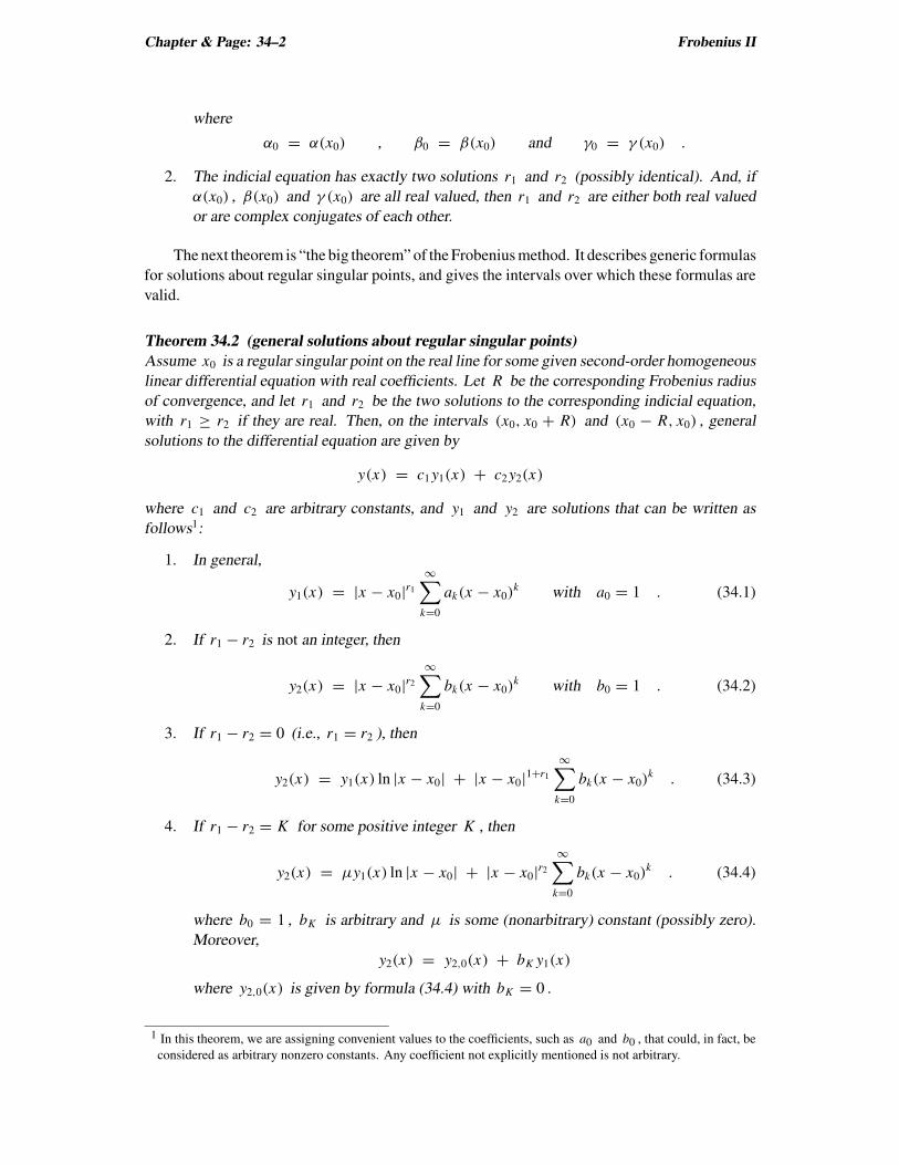
Theorem 34.2 (general solutions about regular singular points)

Assume x0 is a regular singular point on the real line for some given second-order homogeneous

linear differential equation with real coefficients. Let R be the corresponding Frobenius radius

of convergence, and let r1 and r2 be the two solutions to the corresponding indicial equation,

with r1 ≥ r2 if they are real. Then, on the intervals (x0, x0 + R) and (x0 − R, x0) , general

solutions to the differential equation are given by

y(x) = c1 y1(x) + c2 y2(x)

where c1 and c2 are arbitrary constants, and y1 and y2 are solutions that can be written as

follows1:

1. In general,

y1(x) = |x − x0|r1

∞∑

k=0

ak(x − x0)k with a0 = 1 . (34.1)

2. If r1 − r2 is not an integer, then

y2(x) = |x − x0|r2

∞∑

k=0

bk(x − x0)k with b0 = 1 . (34.2)

3. If r1 − r2 = 0 (i.e., r1 = r2 ), then

y2(x) = y1(x) ln |x − x0| + |x − x0|1+r1

∞∑

k=0

bk(x − x0)k . (34.3)

4. If r1 − r2 = K for some positive integer K , then

y2(x) = µy1(x) ln |x − x0| + |x − x0|r2

∞∑

k=0

bk(x − x0)k . (34.4)

where b0 = 1 , bK is arbitrary and µ is some (nonarbitrary) constant (possibly zero).

Moreover,

y2(x) = y2,0(x) + bK y1(x)

where y2,0(x) is given by formula (34.4) with bK = 0 .

1 In this theorem, we are assigning convenient values to the coefficients, such as a0 and b0 , that could, in fact, be

considered as arbitrary nonzero constants. Any coefficient not explicitly mentioned is not arbitrary.

The Big Theorems Chapter & Page: 34–3

Alternate FormulasSolutions Corresponding to Integral Exponents

Remember that in developing the basic method of Frobenius, the first solution we obtained was

actually of the form

y1(x) = (x − x0)r1

∞∑

k=0

ak(x − x0)k

and not

y1(x) = |x − x0|r1

∞∑

k=0

ak(x − x0)k

As noted on page 33–23, either solution is valid on both (x0, x0 + R) and on (x0 − R, x0) . It’s

just that the second formula yields a real-valued solution even when x < x0 and r1 is a real

number other than an integer.

Still, if r1 is an integer — be it 8 , 0 , −2 or any other integer — then replacing

(x − x0)r1 with |x − x0|r1

is completely unnecessary, and is usually undesirable. This is especially true if r1 = n for some

nonnegative integer n , because then

y1(x) = (x − x0)n

∞∑

k=0

ak(x − x0)k =

∞∑

k=0

ak(x − x0)k+n

is actually a power series about x0 , and the proof of theorem 34.2 (given later) will show that

this is a solution on the entire interval (x0 − R, x0 + R) . It might also be noted that, in this case,

y1 is analytic at x0 , a fact that might be useful in some applications.

Similar comments hold if the other exponent, r2 , is an integer. So let us make official:

Corollary 34.3 (solutions corresponding to integral exponents)

Let r1 and r2 be as in theorem 34.2.

1. If r1 is an integer, then the solution given by formula (34.1) can be replaced by the

solution given by

y1(x) = (x − x0)r1

∞∑

k=0

ak(x − x0)k with a0 = 1 . (34.5)

2. If r2 is an integer while r1 is not, then the solution given by formula (34.2) can be

replaced by the solution given by

y2(x) = (x − x0)r2

∞∑

k=0

bk(x − x0)k with b0 = 1 . (34.6)

3. If r1 = r2 and are integers, then the solution given by formula (34.3) can be replaced by

the solution given by

y2(x) = y1(x) ln |x − x0| + (x − x0)1+r1

∞∑

k=0

bk(x − x0)k . (34.7)


4. If r1 and r2 and are two different integers, then the solution given by formula (34.4) can

be replaced by the solution given by

y2(x) = µy1(x) ln |x − x0| + (x − x0)r2

∞∑

k=0

bk(x − x0)k . (34.8)

Other Alternate Solutions Formulas

It should also be noted that alternative versions of formulas (34.3) and (34.4) can be found by

simply factoring out y1(x) from both terms, giving us

y2(x) = y1(x)

[

ln |x − x0| + (x − x0)1

∞∑

k=0

ck(x − x0)k

]

(34.3 ′)

when r2 = r1 , and

y2(x) = y1(x)

[

µ ln |x − x0| + (x − x0)−K

∞∑

k=0

ck(x − x0)k

]

(34.4 ′)

when r1 − r2 = K for some positive integer K . In both cases, c0 = b0 .

Theorem 34.2 and the Method of Frobenius

Remember that, using the basic method of Frobenius, we can find every solution of the form

y(x) = |x − x0|r∞

∑

k=0

ak(x − x0)k with a0 6= 0 ,

provided, of course, such solutions exist. Fortunately for us, statement 1 in the above theorem

assures us that such solutions will exist corresponding to r1 . This means our basic method

of Frobenius will successfully lead to a valid first solution (at least when the coefficients of

the differential equation are rational). Whether there is a second solution y2 of this form

depends:

1. If r1 − r2 is not an integer, then statement 2 of the theorem states that there is such a

second solution. Consequently, step 8 of the method will successfully lead to the desired

result.

2. If r1 − r2 is a positive integer, then there might be such a second solution, depending on

whether or not µ = 0 in formula (34.4). If µ = 0 , then formula (34.4) for y2 reduces to

the sort of modified power series we are seeking, and step 8 in the Frobenius method will

give us this solution. What’s more, as indicated in statement 4 of the above theorem, in

carrying out step 8, we will also rederive the solution already obtained in steps 7 (unless

we set bK = 0 )!

On the other hand, if µ 6= 0 , then it follows from the above theorem that no such

second solution exists. As a result, all the work carried out in step 8 of the basic Frobenius

Local Behavior of Solutions: Issues Chapter & Page: 34–5

method will lead only to a disappointing end; namely, that the terms “blow up” (as

discussed in the subsection Problems Possibly Arising in Step 8 starting on page 33–28).2

3. Of course, if r2 = r1 , then the basic method of Frobenius cannot yield a second solution

different from the first. But our theorem does assure us that we can use formula (34.3)

for y2 (once we figure out the values of the bk’s ).

So what can we do if the basic method of Frobenius does not lead to the second solution

y2(x) ? At this point, we have two choices, both using the formula for y1(x) already found by

the basic Frobenius method:

1. Use the reduction of order method.

2. Plug formula (34.3) or (34.4), as appropriate, into the differential equation, and solve for

the bk’s (and, if appropriate, µ ).

In practice — especially if all you have for y1(x) is the modified power series solution from

the basic method of Frobenius — you will probably find that the second of the above choices to

be the better choice. It does lead, at least, to a usable recursion formula for the bk’s . We will

discuss this further in section 34.6.

However, as we’ll discuss in the next few sections, you might not need to find that y2 .

34.2 Local Behavior of Solutions: Issues

In many situations, we are interested in knowing something about the general behavior of a

solution y(x) to a given differential equation when x is at or near some point x0 . Certainly,

for example, we were interested in what y(x) and y′(x) became as x → x0 when considering

initial value problems.

In other problems (which we will see later), x0 may be an endpoint of an interval of interest,

and we may be interested in a solution y only if y(x) and its derivatives remain well behaved

(e.g., finite) as x → x0 . This can become a very significant issue when x0 is a singular point

for the differential equation in question.

In fact, there are two closely related issues that will be of concern:

1. What does y(x) approach as x → x0 ? Must it be zero? Can it be some nonzero finite

value? Or does y(x) “blow up” as x → x0 ? (And what about the derivatives of y(x)

as x → x0 ?)

2. Can we treat y as being analytic at x0 ?

Of course, if y is analytic at x0 , then, for some R > 0 , it can be represented by a power series

y(x) =∞

∑

k=0

ck(x − x0)k for |x − x0| < R ,

2 We will find a formula for µ in the next chapter. Unfortunately, it is not a simple formula, and is not of much help

in preventing us from attempting step 8 of the basic Frobenius method when that step does not lead to y2 .


and, as we already know,

limx→x0

y(x) = y(x0) = c0 and limx→x0

y′(x) = y′(x0) = c1 .

Thus, when y is analytic at x0 , the limits in question are “well behaved”, and the question of

whether y(x0) must be zero or can be some nonzero value reduces to the question of whether

c0 is or is not zero.

In the next two sections, we will examine the possible behavior of solutions to a differential

equation near a regular singular point for that equation. Our ultimate interest will be in deter-

mining when the solutions are “well behaved” and when they are not. Then, in section 34.5, we

will apply our results to an important set of equations from mathematical physics, the Legendre

equations.

34.3 Local Behavior of Solutions: Limits at RegularSingular Points

As just noted, a major concern in many applications is the behavior of a solution y(x) as x

approaches a regular singular point x0 . In particular, it may be important to know whether

limx→x0

y(x)

is zero, some finite nonzero value, infinite, or completely undefined.

We discussed this issue at the beginning of chapter 31 for the shifted Euler equation

(x − x0)2α0 y′′ + (x − x0)β0 y′ + γ0 y = 0 . (34.9)

Let us try using what we know about those solutions after comparing them with the solutions

given in our big theorem for

(x − x0)2α(x)y′′ + (x − x0)β(x)y′ + γ (x)y = 0 (34.10)

assuming

α0 = α(x0) , β0 = β(x0) and γ0 = γ (x0) .

Remember, these two differential equations have the same indicial equation

α0r(r − 1) + β0r + γ0 = 0 .

Naturally, we’ll further assume α , β and γ are analytic at x0 with α(x0) 6= 0 so we

can use our theorems. Also, in the following, we will let r1 and r2 be the two solutions to the

indicial equation, with r1 ≥ r2 if they are real.

Preliminary Approximations

Observe that each of the solutions described in theorem 34.2 involves one or more power series

∞∑

k=0

ck(x − x0)k = c0 + c1(x − x0) + c2(x − x0)

2 + c3(x − x0)3 + · · ·

Local Behavior of Solutions: Limits at Regular Singular Points Chapter & Page: 34–7

where c0 6= 0 . As we’ve noted in earlier chapters,

limx→x0

∞∑

k=0

ck(x − x0)k = lim

x→x0

[

c0 + c1(x − x0) + c2(x − x0)2 + · · ·

]

= c0 .

This means∞

∑

k=0

ck(x − x0)k ≈ c0 when x ≈ x0 .

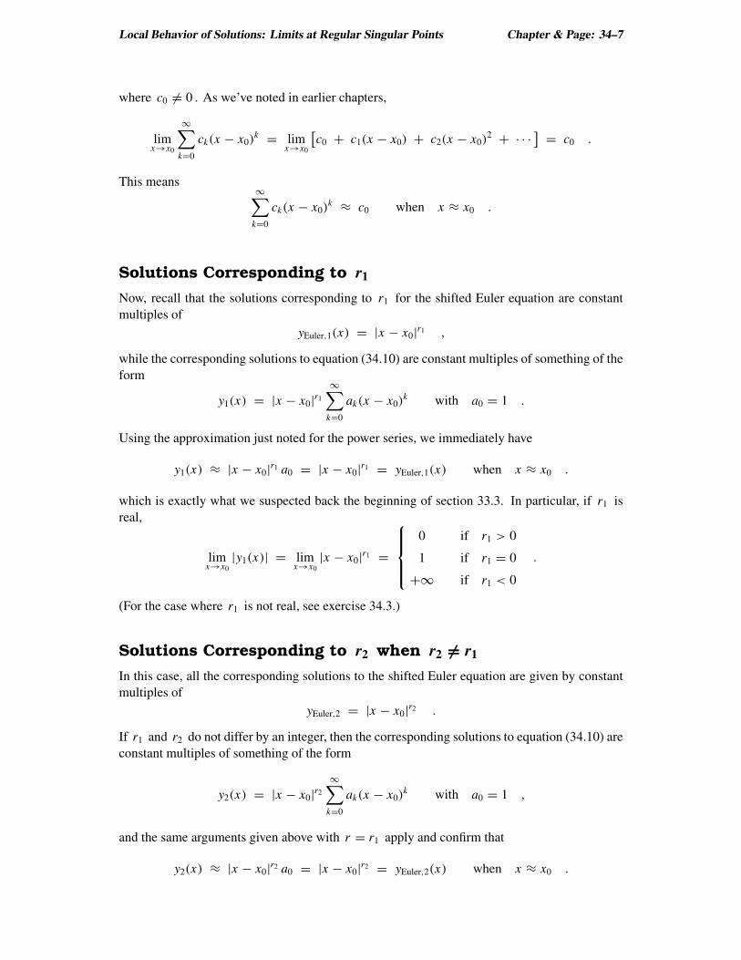
Solutions Corresponding to r1

Now, recall that the solutions corresponding to r1 for the shifted Euler equation are constant

multiples of

yEuler,1(x) = |x − x0|r1 ,

while the corresponding solutions to equation (34.10) are constant multiples of something of the

form

y1(x) = |x − x0|r1

∞∑

k=0

ak(x − x0)k with a0 = 1 .

Using the approximation just noted for the power series, we immediately have

y1(x) ≈ |x − x0|r1 a0 = |x − x0|r1 = yEuler,1(x) when x ≈ x0 .

which is exactly what we suspected back the beginning of section 33.3. In particular, if r1 is

real,

limx→x0

|y1(x)| = limx→x0

|x − x0|r1 =

0 if r1 > 0

1 if r1 = 0

+∞ if r1 < 0

.

(For the case where r1 is not real, see exercise 34.3.)

Solutions Corresponding to r2 when r2 6= r1

In this case, all the corresponding solutions to the shifted Euler equation are given by constant

multiples of

yEuler,2 = |x − x0|r2 .

If r1 and r2 do not differ by an integer, then the corresponding solutions to equation (34.10) are

constant multiples of something of the form

y2(x) = |x − x0|r2

∞∑

k=0

ak(x − x0)k with a0 = 1 ,

and the same arguments given above with r = r1 apply and confirm that

y2(x) ≈ |x − x0|r2 a0 = |x − x0|r2 = yEuler,2(x) when x ≈ x0 .


On the other hand, if r1 −r2 = K for some positive integer K , then the corresponding solutions

to (34.10) are constant multiples of something of the form

y2(x) = µy1(x) ln |x − x0| + |x − x0|r2

∞∑

k=0

bk(x − x0)k with b1 = 1 .

Using approximations already discussed, we have, when x ≈ x0 ,

y2(x) ≈ µ |x − x0|r1 ln |x − x0| + |x − x0|r2 b0

= µ |x − x0|r2+K ln |x − x0| + |x − x0|r2

= |x − x0|r2[

µ |x − x0|K ln |x − x0| + 1]

.

But K is a positive integer, and you can easily show, via L’Hôpital’s rule, that

limx→x0

(x − x0)K ln |x − x0| = 0 .

Thus, when x ≈ x0 ,

y2(x) ≈ |x − x0|r2 [µ · 0 + 1] = |x − x0|r2 ,

confirming that, whenever r2 6= r1

y2(x) ≈ yEuler,2(x) when x ≈ x0 .

In particular, if r2 is real,

limx→x0

|y2(x)| = limx→x0

|x − x0|r1 =

0 if r2 > 0

1 if r2 = 0

+∞ if r2 < 0

.

Solutions Corresponding to r2 when r2 = r1

In this case, all the second solutions to the shifted Euler equation are constant multiples of

yEuler,2 = |x − x0|r2 ln |x − x0| ,

and the corresponding solutions to our original differential equation are constant multiples of

y2(x) = y1(x) ln |x − x0| + |x − x0|1+r1

∞∑

k=0

bk(x − x0)k .

If x ≈ x0 , then

y2(x) ≈ |x − x0|r1 ln |x − x0| + |x − x0|1+r1 b0

= |x − x0|r1 ln |x − x0|[

1 + |x − x0|ln |x − x0|

b0

]

.

But

limx→x0

|x − x0|ln |x − x0|

= 0 .

Local Behavior of Solutions: Limits at Regular Singular Points Chapter & Page: 34–9

Consequently, when x ≈ x0 ,

y2(x) ≈ |x − x0|r1 ln |x − x0| [1 + 0 · b0] = |x − x0|r1 ln |x − x0| ,

confirming that, again, we have

y2(x) ≈ yEuler,2(x) when x ≈ x0 .

Taking the limit (possibly using L’Hôpital’s rule), you can then easily show that

limx→x0

|y2(x)| = limx→x0

|a0| |x − x0|r1 |ln |x − x0|| =

{

0 if r1 > 0

+∞ if r1 ≤ 0.

!◮Example 34.1 (Bessel’s equation of order 1): Suppose we are only interested in those

solutions on (0,∞) to Bessel’s equation of order 1 ,

x2 y′′ + xy′ +(

x2 − 1)

y = 0 ,

that do not “blow up” as x → 0 .

First of all, observe that this equation is already in the form

(x − x0)2α(x)y′′ + (x − x0)β(x)y′ + γ (x)y = 0

with x0 = 0 , α(x) = 1 , β(x) = 1 and γ (x) = x2 − 1 . So x0 = 0 is a regular singular

point for this differential equation, and the indicial equation,

α0r(r − 1) + β0r + γ0 = 0 ,

is

1 · r(r − 1) + 1 · r − 1 = 0 .

This simplifies to

r 2 − 1 = 0 ,

and has solutions r = ±1 . Thus, the exponents for our differential equation are

r1 = 1 and r2 = −1 .

By the analysis given above, we know that all solutions corresponding to r1 are constant

multiples of one particular solution y1 satisfying

limx→x0

|y1(x)| = limx→x0

|x − x0|1 = 0 .

So none of the solutions corresponding to r = 1 blow up as x → 0 .

On the other hand, the analysis given above for solutions corresponding to r2 when

r2 6= r1 tells us that all the (nontrivial) second solutions are (nonzero) constant multiples of

one particular solution y2 satisfying

limx→x0

|y2(x)| = limx→x0

|x − x0|−1 = ∞ .

And these do “blow up” as x → 0 .

Thus, since we are only interested in the solutions that do not blow up as x → 0 , we need

only concern ourselves with those solutions corresponding to r1 = 1 . Those corresponding

to r2 = −1 are not relevant, and we need not spend time and effort finding their formulas.


Derivatives

To analyze the behavior of the derivative y′(x) as x → x0 , you simply differentiate the modified

power series for y(x) , and then apply the ideas described above. I’ll let you do it in exercise

34.4 at the end of the chapter.

34.4 Local Behavior: Analyticity and Singularities inSolutions

It is certainly easier to analyze how y(x) or any of it’s derivatives behave as x → x0 when

y(x) is given by a basic power series about x0

y(x) =∞

∑

k=0

ck(x − x0)k .

Then, in fact, y is infinitely differentiable at x0 , and we know

limx→x0

y(x) = y(x0) = c0

and

limx→x0

y(x) = y(k) (x0) = k! ck for k = 1, 2, 3, . . . .

On the other hand, if y(x) is given by one of those modified power series described the

big theorem, then, as we partly saw in the last section, computing the limits of y(x) and its

derivatives as x → x0 is much more of a challenge. Indeed, unless that series is of the form

(x − x0)r

∞∑

k=0

αk(x − x0)k

with r being zero or some postive integer, then limx→x0y(x) may blow up or otherwise fail to

exist. And even if that limit does exist, you can easily show that the corresponding limit of the

nth derivative, y(n)(x) , will either blow up or fail to exist if n > r .

To simplify our discussion, let’s slightly expand our “ordinary/singular point” terminology

so that it applies to any function y . Basically, we want to refer to a point x0 as an ordinary

point for a function y if y is analytic at x0 , and we want to refer to x0 as a singular point for

y if y is not analytic at x0 .

There are, however, small technical issues that must be taken into account. Typically, our

function y is defined on some interval (α, β) , possibly by some power series or modified power

series. So, initially at least, we must confine our definitions of ordinary and singular points for

y to points in or at the ends of this interval. To be precise, for any such point x0 , we will say

that x0 is an ordinary point for y if and only if there is a power series∑∞

k=0 ak(x − x0)k with

a nonzero radius of convergence R such that,

y(x) =∞

∑

k=0

ak(x − x0)k

Local Behavior: Analyticity and Singularities in Solutions Chapter & Page: 34–11

for all x in (α, β) with |x − x0| < R . If no such power series exists, then we’ll say x0 is a

singular point for y .

By the way, instead of referring to x0 as an ordinary point for y , we may also refer to x0

as a point of analyticity for y . And we may say that y has a singularity at x0 instead of saying

x0 is a singular point for y .

Our interest, of course, is in the functions that are solutions to differential equations, and,

as we discovered in previous chapters, solutions to the sort of differential equations we are

considering are analytic at the ordinary points of those equations. So we immediately have:

Lemma 34.4

Let y be a solution on an interval (α, β) to some second-order homogeneous differential equa-

tion, and let x0 be either in (α, β) or be one of the endpoints. Then

x0 is an ordinary point for the differential equation H⇒ x0 is an ordinary point for y .

Equivalently,

x0 is a singular point for y H⇒ x0 is a singular point for the differential equation .

This lemma does not say that y must have a singularity at each singular point of the

differential equation. After all, if x0 is a regular singular point, and the first solution r1 of the

indicial equation is a nonnegative integer, say, r1 = 3 , then our big theorem assures us of a

solution y1 given by

y1(x) = (x − x0)3

∞∑

k=0

ak(x − x0)k ,

which is a true power series since

(x − x0)3

∞∑

k=0

ak(x − x0)k =

∞∑

k=0

ak(x − x0)k+3 =

∞∑

n=0

ck(x − x0)n

where

cn =

{

0 if n < 3

an−3 if n ≥ 3.

Still, there are cases where one can be sure that a solution y to a given second-order linear

homogeneous differential equation has at least one singular point. In particular, consider the

situation in which y is given by a power series

y(x) =∞

∑

k=0

ck(x − x0)k for |x − x0| < R

when R is the radius of convergence, and is finite. Replacing x with the complex variable z ,

y(z) =∞

∑

k=0

ck(z − x0)k

yields a power series with radius of convergence R for a complex-variable function y(z) analytic

at least on the disk of radius R about z0 . Now, it can be shown that there must then be a point


zs on the edge of this disk at which y(z) is not “well behaved”. Unsurprisingly, it can also be

shown that this zs is a singular point for the differential equation. And if all the singular points

of this differential equation happen to lie on the real line, then this singular point zs must be one

of the two points on the real line satisfying |zs − x0| = R , namely,

zs = x0 − R or zs = x0 + R .

That gives us the following theorem (which we will find useful in the following section and in

some of the exercises).

Theorem 34.5

Let x0 be a point on the real line, and assume

y(x) =∞

∑

k=0

ck(x − x0)k for |x − x0| < R

is a power power series solution to some homogeneous second-order differential equation. Sup-

pose further, that both of the following hold:

1. R is the radius of convergence for the above power series and is finite.

2. All the singular points for the differential equation are on the real axis.

Then at least one of the two points x0 − R or x0 + R is a singular point for y .

Admittedly, our derivation of the above theorem was rather sketchy and involved claims that

“can be shown”. If that isn’t good enough for you, then turn to section 34.7 for a more satisfying

proof. There will be pictures.

34.5 A Case Study: The Legendre Equations

As an application of what we have just developed, let us analyze the behavior of the solutions to

the set of Legendre equations. These equations often arise in physical problems in which some

spherical symmetry can be expected, and in most applications (for reasons I cannot explain here3

only those solutions that are “bounded” on (−1, 1) are of interest. Our analysis here will allow

us to readily find those solutions, and will save us from a lot of needless work dealing with those

solutions that, ultimately, will not be of interest.

Let me remind you of what a Legendre equation is; it is any differential equation that can

be written as

(1 − x2)y′′ − 2xy′ + λy = 0 (34.11)

where λ , the equation’s parameter, is some constant. You may recall these equations from

exercise 31.9 on page 31–41, and we will begin our analysis here by recalling what we learned

in that rather lengthy exercise.

3 With luck, some of the reasons will be explained in a later chapter on “boundary-value problems” .

A Case Study: The Legendre Equations Chapter & Page: 34–13

What We Already Know

In that exercise 31.9 on page 31–41, you (I hope) discovered the following:

1. The only singular points for each Legendre equation are x = −1 and x = 1 .

2. For each λ , a general solution on (−1, 1) of Legendre equation (34.11) is

yλ(x) = a0 yλ,E(x) + a1 yλ,O(x)

where yλ,E(x) is a power series about 0 having just even-powered terms and whose first

term is 1 , and yλ,O(x) is a power series about 0 having just odd-powered terms and

whose first term is x ,

3. If λ = m(m + 1) for some nonnegative integer m , then the Legendre equation with

parameter λ has polynomial solutions, all of which are constant multiples of the m th

degree polynomial pm(x) where

p0(x) = y0,E(x) = 1 ,

p1(x) = y2,O(x) = x ,

p2(x) = y6,E(x) = 1 − 3x2 ,

p3(x) = y12,O(x) = x − 5

3x3 ,

p4(x) = y20,E(x) = 1 − 10x2 + 35

3x4 ,

p5(x) = y30,O(x) = x − 14

3x3 + 21

5x5

and, in general,

pm(x) ={

yλ,E(x) if m is even

yλ,O(x) if m is odd.

4. The Legendre equation with parameter λ has no polynomial solution on (−1, 1) if

λ 6= m(m + 1) for every nonnegative integer m

5. If y is a nonpolynomial solution to a Legendre equation on (−1, 1) , then it is given by

a power series about x0 = 0 with a radius of convergence of exactly 1 .

Let us now see what more we can determine about the solutions to the Legendre equations

on (−1, 1) using the material developed in the last few sections. For convenience, we will

record the noteworthy results as we derive them in a series of lemmas which, ultimately, will be

summarized in a major theorem on Legendre equations, theorem 34.11.

The Singular Points of the Solutions

First of all, we should note that, because polynomials are analytic everywhere, the polynomial

solutions to Legendre’s equation have no singular points.

Now, suppose y is a solution to a Legendre equation, but is not a polynomial. As noted

above, y(x) can be given by a power series about x0 = 0 with radius of convergence 1 . This,


and the fact that the only singular points for Legendre’s equation are the points x = −1 and

x = 1 on the real line, means that lemma 34.5 applies and immediately gives us the following:

Lemma 34.6

Let y be a nonpolynomial solution to a Legendre equation on (−1, 1) . Then y must have a

singularity at either x = −1 or at x = 1 (or both).

Solution Limits at x = 1

To determine the limits of the solutions at x = 1 , we will first find the exponents of the Legendre

equation at x = 1 by solving the appropriate indicial equation. To do this, it is convenient to

first multiply the Legendre equation by −1 and factor the first coefficient, giving us

(x − 1)(x + 1)y′′ + 2xy′ − λy = 0 .

Multiplying this by x − 1 converts the equation into “standard form”,

(x − 1)2α(x)y′′ + (x − 1)β(x)y′ + γ (x)y = 0

where

α(x) = x + 1 , β(x) = 2x and γ (x) = −(x − 1)λ .

Thus, the corresponding indicial equation is

r(r − 1)α0 + rβ0 + γ0 = 0

with

α0 = α(1) = 2 , β0 = β(1) = 2 and γ0 = γ (1) = 0 .

That is, the exponents r = r1 and r = r2 must satisfy

r(r − 1)2 + 2r = 0 ,

which simplifies to r 2 = 0 . So,

r1 = r2 = 0 ,

and our big theorem on the Frobenius method, theorem 34.2 on page 34–2, tells us that any

solution y to a Legendre equation on (−1, 1) can be written as

y(x) = c+1 y+

1 (x) + c+2 y+

2

where

y+1 (x) = |x − 1|0

∞∑

k=0

a+k (x − 1)k =

∞∑

k=0

a+k (x − 1)k with a+

0 = 1 ,

and

y+2 (x) = y+

1 (x) ln |x − 1| + (x − 1)

∞∑

k=0

b+k (x − 1)k .

Now, let’s make some simple observations using these formulas:

A Case Study: The Legendre Equations Chapter & Page: 34–15

1. The point x = 1 is an ordinary point for the solution y+1 . Moreover

limx→1

y+1 (x) = a+

0 = 1 .

2. On the other hand, because of the logarithmic factor in y+2 ,

limx→1

y+2 (x) = 1 · lim

x→1ln |x − 1| + (1 − 1)b+

0 = −∞ .

Hence, x = 1 is not an ordinary point for y+2 ; it is a singular point for that solution.

3. More generally, if y(x) = c+1 y+

1 (x) + c+2 y+

2 (x) is any nontrivial solution to Legendre’s

equation on (−1, 1) , then the following must hold:

(a) If c+2 6= 0 , then x = 1 is a singular point for y , and

limx→1

|y(x)| =∣∣∣ c+

1 limx→1

y+1 (x)

︸︷︷︸

1

+ c+2 lim

x→1y+

2 (x)

︸︷︷︸

−∞

∣∣∣ = ∞ .

(b) If c+2 = 0 , then c+

1 6= 0 , and x = 1 is an ordinary point for y . Moreover,

limx→1

y(x) = c+1 lim

x→1y+

1 (x) = c+1 6= 0 .

(Hence, x = 1 is a singular point for y if and only if c+2 6= 0 .)

All together, these observations give us:

Lemma 34.7

Let y be a nontrivial solution on (−1, 1) to Legendre’s equation. Then x = 1 is a singular

point for y if and only if

limx→1−

|y(x)| = ∞ .

Moreover, if x = 1 is not a singular point for y , then

limx→1−

y(x)

exists and is a finite nonzero value.

Solution Limits at x = −1

A very similar analysis using x = −1 instead of x = 1 leads to:

Lemma 34.8

Let y be a nontrivial solution on (−1, 1) to Legendre’s equation. Then x = −1 is a singular

point for y if and only if

limx→−1+

|y(x)| = ∞ .

Moreover, if x = −1 is not a singular point for y , then

limx→−1+

y(x)

exists and is a finite nonzero value.


?◮Exercise 34.1: Verify the above lemma by redoing the analysis done in the previous

subsection using x = −1 in place of x = 1 .

The Unboundedness of the Nonpolynomial Solutions

Recall that a function y is said to be bounded on an interval (a, b) if there is a finite number

M which “bounds” the absolute value of y(x) when x is in (a, b) ; that is,

|y(x)| ≤ M whenever a < x < b .

Naturally, if a function is not bounded on the interval of interest, we say it is unbounded.

Now, if y happens to be one of those nonpolynomial solutions to a Legendre equation on

(−1, 1) , then we know y has a singularity at either x = −1 or at x = 1 or at both (lemma

34.6). Lemmas 34.7 and 34.8 then tell us that

limx→1−

|y(x)| = ∞ or limx→−1+

|y(x)| = ∞ ,

clearly telling us that y(x) is not bounded on (−1, 1) !

Lemma 34.9

Let y be a nonzero solution to a Legendre equation on (−1, 1) . If y is not a polynomial, then

it is not bounded on (−1, 1) .

The Polynomial Solutions and Legendre Polynomials

Now assume y is a nonzero polynomial solution to a Legendre eqaution.

First of all, because each polynomial is a continuous function on the real line, we know from

a classic theorem of calculus that the polynomial has maximum and minimum values over any

given closed subinterval. Thus, in particular, our polynomial solution y has a maximum and a

minimum value over [−1, 1] , and, hence, is bounded on (−1, 1) . So

Lemma 34.10

Each polynomial solution to a Legendre equation is bounded on (−1, 1) .

But now remember that the Legendre equation with parameter λ has polynomial solutions if

and only if λ = m(m + 1) for some nonnegative integer m , and those solutions are all constant

multiples of

pm(x) =

{



Since x = 1 is not a singular point for pm , lemma 34.7 tells us that

pm(1) = limx→1

pm(1) 6= 0 .

This allows us to define the m th Legendre polynomial Pm by

Pm(x) = 1

pm(1)pm(x) for m = 0, 1, 2, 3, . . . .

Finding Second Solutions Using Theorem 34.2 Chapter & Page: 34–17

Clearly, any constant multiple of pm is also a constant multiple of Pm . So we can use the Pm’s

instead of the pm’s to describe all polynomial solutions to the Legendre equations.

In practice, it is more common to use the Legendre polynomials than the pm’s . In part, this

is because

Pm(1) = 1

pm(1)pm(1) = 1 for m = 0, 1, 2, 3, . . . .

With a little thought, you’ll realize that this means that, for each nonnegative integer m , Pm is

the polynomial solution to the Legendre equation with parameter λ = m(m + 1) that equals 1

when x = 1 .

Summary

This is a good time to skim the lemmas in this section, along with the discussion of the Legendre

polynomials, and verify for yourself that these results can be condensed into the following:

Theorem 34.11 (bounded solutions of the Legendre equations)

There are bounded, nontrivial solutions on (−1, 1) to the Legendre equation

(1 − x2)y′′ − 2xy′ + λy = 0

if and only if λ = m(m + 1) for some nonnegative integer m . Moreover, y is such a solution

if and only if y is a constant multiple of the m th Legendre polynomial.

We may find a use for this theorem in a later chapter.

34.6 Finding Second Solutions Using Theorem 34.2

Let’s return to actually solving differential equations.

When the basic method of Frobenius fails to deliver a second solution, we can turn to the

appropriate formulas given in theorem 34.2 on page 34–2; namely, formula (34.3),

y2(x) = y1(x) ln |x − x0| + |x − x0|1+r1

∞∑

k=0

bk(x − x0)k

or formula (34.4),

y2(x) = µy1(x) ln |x − x0| + |x − x0|r2

∞∑

k=0

bk(x − x0)k ,

depending, respectively, on whether the exponents r1 and r2 are equal or differ by a nonzero

integer (the only cases for which the basic method might fail). The unknown constants in these

formulas can then be found by fairly straightforward variations of the methods we’ve already

developed: Plug formula (34.3) or (34.4) (as appropriate) into the differential equation, derive

the recursion formula for the bk’s (and the value of µ if using formula (34.4)), and compute as

many of the bk’s as desired.

Because the procedures are straightforward modifications of what we’ve already done many

times in the last few chapters, we won’t describe the steps in detail. Instead, we’ll illustrate the


basic ideas with an example, and then comment on those basic ideas. As you’ve come to expect

in these last few chapters, the computations are simple but lengthy. But do note how the linearity

of the equations is used to break the computations into more digestible pieces.

The Second Solution When r1 − r2 Is a Positive Integer

!◮Example 34.2: In example 33.9, starting on page 33–29, we attempted to find modified

power series solutions about x0 = 0 to

2xy′′ − 4y′ − y = 0 ,

which we rewrote as

2x2 y′′ − 4xy′ − xy = 0 .

We found the exponents of this equation to be

r1 = 3 and r2 = 0 ,

and obtained

y(x) = cx3

∞∑

k=0

6

2k k!(k + 3)!xk (34.12)

as the solutions to the differential equation corresponding to r1 . Unfortunately, we found that

there was not a similar solution corresponding to r2 .

To apply theorem 34.2, we first need the particular solution corresponding to r1

y1(x) = x3

∞∑

k=0

ak xk with a0 = 1 .

So we use formula (34.12) with c chosen so that

c6

20 0!(0 + 3)!︸︷︷︸

a0

= 1 .

Simple computations show that c = 1 and, so,

y1(x) = x3

∞∑

k=0

6

2k k!(k + 3)!xk =

∞∑

k=0

6

2k k!(k + 3)!xk+3 .

According to theorem 34.2, the general solution to our differential equation is

y(x) = c1 y1(x) + c2 y2(x)

where y1 is as above, and (since r2 = 0 and K = r1 − r2 = 3 )

y2(x) = µy1(x) ln |x − x0| +∞

∑

k=0

bk xk .

where b0 = 1 , b3 is arbitrary (we’ll take it to be zero), and µ is some constant. To simplify

matters, let us rewrite the last formula as

y2(x) = µY1(x) + Y2(x)

Finding Second Solutions Using Theorem 34.2 Chapter & Page: 34–19

where

Y1(x) = y1(x) ln |x | and Y2(x) =∞

∑

k=0

bk xk .

Thus,

0 = 2x2 y1′′ − 4x y1

′ − xy1

= 2x2[µY1 + Y2]′′ − 4x[µY1 + Y2]′ − x[µY1 + Y2] .

By the linearity of the derivatives, this can be rewritten as

0 = µ{

2x2Y1′′ − 4xY1

′ − xY1

}

+{

2x2Y2′′ − 4xY2

′ − xY2

}

. (34.13)

Now, because y1 is a solution to our differential equation, you can easily verify that

2x2Y1′′ − 4xY1

′ − xY1

= 2x2 d2

dx2[y1(x) ln |x |] − 4x

d

dx[y1(x) ln |x |] − x [y1(x) ln |x |]

= · · ·= 4x y1

′ − 6y1 .

Replacing the y1 in the last line with its series formula then gives us

2x2Y1′′ − 4xY1

′ − xY1 = 4xd

dx

∞∑

k=0

6

2k k!(k + 3)!xk+3 − 6

∞∑

k=0

6

2k k!(k + 3)!xk+3 ,

which, after suitable computation and reindexing (you do it), becomes

2x2Y1′′ − 4xY1

′ − xY1 =∞

∑

n=3

12(2n − 3)

2n−3(n − 3)!n!xn . (34.14)

Next, using the series formula for Y2 we have

2x2Y2′′ − 4xY2

′ − xY2 = 2x2 d2

dx2

∞∑

k=0

bk xk − 4xd

dx

∞∑

k=0

bk xk − x

∞∑

k=0

bk xk ,

which, after suitable computations and changes of indices (again, you do it!), reduces to

2x2Y2′′ − 4xY2

′ − xY2 =∞

∑

n=1

{2n(n − 3)bn − bn−1} xn . (34.15)

Combining equations (34.13), (34.14) and (34.15):

0 = µ{

2x2Y1′′ − 4xY1

′ − xY1

}

+{

2x2Y2′′ − 4xY2

′ − xY2

}

= µ

∞∑

n=3

12(2n − 3)

2n−3(n − 3)!n!xn +

∞∑

n=1

{2n(n − 3)bn − bn−1} xn

= µ

∞∑

n=3

12(2n − 3)

2n−3(n − 3)!n!xn +

{

[−4b1 − b0]x1 + [−4b2 − b1]x2

+∞

∑

n=3

{2n(n − 3)bn − bn−1} xn

}


= −[4b1 + b0]x1 − [4b2 + b1]x2

+∞

∑

n=3

[

2n(n − 3)bn − bn−1 + µ12(2n − 3)

2n−3(n − 3)!n!

]

xn .

Since each term in this last power series must be zero, we must have

−[4b1 + b0] = 0 , − [4b2 + b1] = 0

and

2n(n − 3)bn − bn−1 + µ12(2n − 3)

2n−3(n − 3)!n!= 0 for n = 3, 4, 5, . . . .

This (and the fact that we’ve set b0 = 1 ) means that

b1 = −1

4b0 = −1

4· 1 = −1

4, b2 = −1

4b1 = −1

4

(

−1

4

)

= 1

16

and

2n(n − 3)bn = bn−1 − µ12(2n − 3)

2n−3(n − 3)!n!for n = 3, 4, 5, . . . . (34.16)

Because of the n − 3 factor in front of bn , dividing the last equation by 2n(n − 3) to get a

recursion formula for the bn’s would result in a recursion formula that ”blow ups” for n = 3 .

So we need to treat that case separately.

With n = 3 in equation (34.16), we get

2 · 3(3 − 3)b3 = b2 − µ12(2 · 3 − 3)

23−3(3 − 3)!3!

→֒ 0 = 1

16− µ6

→֒ µ = 1

96.

Notice that we obtained the value for µ instead of b3 . As claimed in the theorem, b3 is

arbitrary. Because of this, and because we only need one second solution, let us set

b3 = 0 .

Now we can divide equation (34.16) by 2n(n − 3) and use the value for µ just derived

(with a little arithmetic) to obtain the recursion formula

bn = 1

2n(n − 3)

[

bn−1 − (2n − 3)

2n(n − 3)!n!

]

for n = 4, 5, 6, . . . .

So,

b4 = 1

2 · 4(4 − 3)

[

b3 − (2 · 4 − 3)

24(4 − 3)!4!

]

= 1

8

[

0 − 5

384

]

= − 5

3,072,

b5 = 1

2 · 5(5 − 3)

[

b4 + (2 · 5 − 3)

25(5 − 3)!5!

]

= 1

20

[

−5

3,072+ 7

7,680

]

= − 11

307,200,

...

Appendix on Proving Theorem 34.5 Chapter & Page: 34–21

We won’t attempt to find a general formula for the bn’s here!

Thus, a second particular solution to our differential equation is

y2(x) = µy1(x) ln |x − x0| +∞

∑

k=0

bk xk

= 1

96y1(x) ln |x | +

{

1 − 1

4x + 1

16x2 + 0x3 − 5

3,072x4 − 11

307,200x5 + · · ·

}

where y1 is our first particular solution,

y1(x) =∞

∑

k=0

6

2k k!(k + 3)!xk+3 .

In general, when

r1 − r2 = K

for some positive integer K , the computations illustrated in the above example will yield a

second particular solution. It will turn out that b1 , b2 , . . . and bK−1 are all “easily computed”

from b0 , just as in the example. You will also obtain a recursion relation for bn in terms of

lower-indexed bk’s and the coefficients from the series formula for y1 . This recursion formula

(formula (34.16) in our example) will hold for n ≥ K , but be degenerate when n = K (just as

in our example, where K = 3 ). From that degenerate case, the value of µ in formula (34.4)

can be determined. The rest of the bn’s can then be computed using the recursion relation.

Unfortunately, it is highly unlikely that you will be able to find a general formula for these bn’s

in terms of just the index, n . So just compute as many as seem reasonable.

The Second Solution When r1 = r2

The basic ideas illustrated in the last example also apply when the exponents of the differential

equation, r1 and r2 , are equal. Of course, instead of using the formula used in the example for

y2 , use formula (34.3),

y2(x) = y1(x) ln |x − x0| + |x − x0|1+r1

∞∑

k=0

bk(x − x0)k .

In this case, there is no “ µ ” to determine and none of the bk’s will be arbitrary. In some ways,

that makes this a simpler case than considered in our example. I’ll leave it to you to work out

any details in the exercises.

34.7 Appendix on Proving Theorem 34.5

Our goal in this section is to describe how theorem 34.5 on page 34–12 can be rigorously verified.

To aid us, we will first extend some of the material we developed on power series solutions and

complex variables.


Complex Power Series Solutions

Throughout most of these chapters, we’ve been tacitly assuming that the derivatives in our

differential equations are derivatives with respect to a real variable x ,

y′ = dy

dxand y′′ = d2 y

dx2,

as in elementary calculus. In fact, we can also have derivatives with respect to the complex

variable z ,

y′ = dy

dzand y′′ = d2 y

dz2.

The precise definitions for these “complex derivatives” are given in appendix 32.6 (see page 32–

18), where it is pointed out that, computationally, differentiation with respect to z is completely

analogous to the differentiation with respect to x learned in basic calculus. In particular, if

y(z) =∞

∑

k=0

ak(z − z0)k for |z − z0| < R

for some point z0 in the complex plane and some R > 0 , then

y′(z) = d

dz

∞∑

k=0

ak(z − z0)k

=∞

∑

k=0

d

dz

[

ak(z − z0)k]

=∞

∑

k=1

kak(z − z0)k−1 for |z − z0| < R .

Consequently, all of our computations in chapters 31 and 32 can be carried out using the complex

variable z instead of the real variable x , and using a point z0 in the complex plane instead of

a point x0 on the real line. In particular, we have the following complex-variable analog of

theorem 32.9 on page 32–10:

Theorem 34.12 (second-order series solutions)

Suppose z0 is an ordinary point for a second-order homogeneous differential equation whose

reduced form isd2 y

dz2+ P

dy

dz+ Qy = 0 .

Then P and Q have power series representations

P(z) =∞

∑

k=0

pk(z − z0)k for |z − z0| < R

and

Q(z) =∞

∑

k=0

qk(z − z0)k for |z − z0| < R

where R is the radius of analyticity about z0 for this differential equation.

Moreover, a general solution to the differential equation is given by

y(z) =∞

∑

k=0

ak(z − z0)k for |z − z0| < R


z1

z2

z3

DADBD0

D1

D2

D3

ζ

Figure 34.1: Disks in the complex plane for theorem 34.13 and its proof.

where a0 and a1 are arbitrary, and the other ak’s satisfy the recursion formula

ak = − 1

k(k − 1)

k−2∑

j=0

[

( j + 1)a j+1 pk−2− j + a j qk−2− j

]

. (34.17)

By the way, it should also be noted that, if

y(x) =∞

∑

k=0

ck(x − x0)k

is a solution to the real-variable differential equation for |x − x0| < R , then

y(z) =∞

∑

k=0

ck(z − x0)k

is a solution to the corresponding complex-variable differential equation for |z − x0| < R . This

follows immediately from the last theorem and the relation between dy/dx and dy/dz (see the

discussion of the complex derivative in section 32.6).

Analytic Continuation

Analytic continuation is any procedure that “continues” an analytic function defined on one

region so that it becomes defined on a larger region. Perhaps it would be better to call it “analytic

extension” because what we are really doing is extending the domain of our original function

by creating an analytic function with a larger domain that equals the original function over the

original domain.

We’ll use two slightly different methods for doing analytic continuation. Both are based on

Taylor series, and both can justified by the following theorem.

Theorem 34.13

Let DA and DB be two open disks in the complex plane that intersect each other, and let fA

be a function analytic on DA and fB a function analytic on DB . Assume further that there is

an open disk D0 contained in both DA and DB (see figure 34.1), and that

fA(z) = fB(z) for every z ∈ D0 .


Then

fA(z) = fB(z) for every z ∈ DA ∩ DB .

Think of fA as being the original function defined on DA , and fB as some other analytic

function that we constructed on DB to match fA on D0 . This theorem tells us that we can

define a “new” function f on DA ∪ DB by

f (z) =

{

f A(z) if z is in DA

fB(z) if z is in DB

.

On the intersection, f is given both by fA and fB , but that is okay because the theorem assures

us that fA and fB are the same on that intersection. And since fA and fB are, respectively,

analytic at every point in DA and DB , it follows that f is analytic on the union of DA and

DB , and satisfies

f (z) = fA(z) for each z in DA .

That is, f is an “analytic extension” of f A from the domain DA to the domain DA ∪ DB .

The proof of the above theorem is not difficult, and is somewhat instructive.

PROOF (theorem 34.13): We need to show that f A(ζ ) = fB(ζ ) for every ζ in DA ∩ DB .

So let ζ be any point in DA ∩ DB .

If ζ ∈ D0 then, by our assumptions, we automatically have fA(ζ ) = fB(ζ ) .

On the other hand, if ζ in not in D0 , then, as illustrated in figure 34.1, we can clearly find

a finite sequence of open disks D1 , D2 , . . . and DM with respective centers z1 , z2 , . . . and

zM such that

1. each zk is also in Dk−1 ,

2. each Dk is in DA ∩ DB , and

3. the last disk, DM , contains ζ .

Now, because fA and fB are the same on D0 , so are all their derivatives. Consequently,

the Taylor series for f A and fB about the point z1 in D0 will be the same. And since D1 is a

disk centered at z1 and contained in both DA and DB , we have

fA(z) =∞

∑

k=0

f A(k)(z1)

k!(z − z1)

k

=∞

∑

k=0

fB(k)(z1)

k!(z − z1)

k = fB(z) for every z in D1 .

Repeating these arguments using the Taylor series for fA and fB at the points z2 , z3 , and

so on, we eventually get

fA(z) = fB(z) for every z in DM .

In particular then,

fA(ζ ) = fB(ζ ) ,

just as we wished to show.


(a) (b)

z0 D0

D0

DA

DA DB

DB

RB

Xx0a b

Figure 34.2: Disks in the complex plane for (a) corollary 34.14, in which a function on DA

is expanded to a function on DB by a Taylor series at z0 , and (b) corollary

34.15, in which two functions are equal on the interval (a, b) .

One standard way to do analytic continuation is to use the Taylor series of the original

function fA at a point z0 to define the “second” function fB on a disk DB centered at z0

with radius RB . With luck, we can verify that RB can be chosen so that DB extends beyond

the original disk, as in figure 34.2a. Now, since fB is given by the Taylor series of f A at z0 ,

theorem 32.14 on page 32–20 assures us that there is a disk D0 of positive radius about z0 in

DA ∩ DB on which fA and fB are equal (again, see figure 34.2a). A direct application of the

theorem we’ve just proven then gives:

Corollary 34.14

Let fA be a function analytic on some open disk DA of the complex plane, and let z0 be any

point in DA . Set

fB(z) =∞

∑

k

ck(z − z0)k for |z − z0| < RB

where∑∞

k ck(z − z0)k is the Taylor series for fA about z0 and RB is the radius of convergence

for this series. Then


where DB is the disk of radius RB about z0 .

As the next corollary demonstrates, it may be possible to apply theorem 34.13 when the two

functions are only known to be equal over an interval. This will be useful for us.

Corollary 34.15

Let DA and DB be two open disks in the complex plane that intersect each other, and let fA

be a function analytic on DA and fB a function analytic on DB . Assume further that there is

an open interval (a, b) in the real axis contained in both DA and DB , and that

f A(x) = fB(x) for every x ∈ (a, b) .

Then



PROOF: Simply construct the Taylor series for fA and fB at some point x0 in (a, b) (see

figure 34.2b). Since these two functions are equal on this interval, so are their Taylor series at

x0 . Hence, fA = fB on some disk D0 of positive radius about x0 . The claim in the corollary

then follows immediately from theorem 34.13.

Proving Theorem 34.5A Closely Related Lemma

Recall that theorem 34.5 makes a claim about the singular points of a power series solution based

on the radius of convergence of that series. It turns out to be slightly more convenient to first

prove the following lemma making a corresponding claim about the radius of convergence for a

power series solution based on ordinary points of the solution.

Lemma 34.16

Let R be a finite positive value, and assume

y(x) =∞

∑

k=0

ck xk for − R < x < R (34.18)


pose further, that all the singular points for this differential equation are on the real axis, but

that x = −R and x = R are ordinary points for y . Then R is strictly less than the radius of

convergence for the above series.

PROOF: By definition, x = −R and x = R being ordinary points for a function y defined

on (−R, R) means that there is a ρ > 0 and power series about x = −R and x = R ,

∞∑

k=0

c+k (x − R)k and

∞∑

k=0

c−k (x + R)k ,

such that

y(x) =∞

∑

k=0

c+k (x − R)k for R − ρ < x < R

and

y(x) =∞

∑

k=0

c−k (x + R)k for − R < x < −R + ρ .

Now let D− and D+ be the disks about x = −R and x = R , respectively, each with radius

ρ , and let

y+(z) =∞

∑

k=0

c+k (z − R)k for z ∈ D+

and

y−(z) =∞

∑

k=0

c−k (z + R)k for z ∈ D−


0

D+D−

D1

D2

D3

R XR + ǫ−R

z1

z2

z3

Figure 34.3: Disks for the proof of lemma 34.16. The darker disk is the disk on which y is

originally defined.

(see figure 34.3).

Now, consider choosing a finite sequence of disks D1 , D2 , . . . , and DN with respective

centers z1 , z2 , . . . , and zN such that that all the following holds:

1. Each zn is inside the disk of radius R about the origin.

2. The radius of each Dn is no greater than the distance of zn to the real axis.

3. The union of all the disks D1 , D2 , . . . , and DN , along with the disks D− and D+ ,

contains not just the boundary of our original disk D but the “ring” of all z satisfying

R ≤ |z| ≤ R + ǫ

for some positive value ǫ .

With a little thought, you will realize that these points and disks can be so chosen (as illustrated

in figure 34.3).

Next, for each n , let yn be the function given by the Taylor series of y at zn ,

yn(z) =∞

∑

k=0

cn,k(z − zn)k with cn,k = 1

k!y(k)(zn) .

Using the facts that y is a solution to the given differential equation on the disk with |z| < R ,

that the differential equation only has singular points on the real axis, and that Dn does not touch

the real axis, we can apply theorem 34.12 in a straightforward manner to show that the above

defines yn as an analytic function on the entire disk Dn . Repeated use of corollaries 34.14 and

34.15 then shows that any two functions from the set

{y, y+, y−, y1, y2, . . . , yN }


equal each other wherever both are defined. This allows us to define a “new” analytic function

Y on the union of all of our disks via

Y (z) =

y(z) if |z| < R

y+(z) if z ∈ D+

y−(z) if z ∈ D−

yn(z) if z ∈ Dn for n = 1, 2, . . . , N

.

Now, because the union of all of the disks contains the disk of radius R + ǫ about 0 , theorem

32.14 on page 32–20 on the radius of convergence for Taylor series assures us that the Taylor series

for Y about z0 = 0 must have a radius of convergence of at least R + ǫ . But, y(z) = Y (z)

when |z| < R . So y and Y have the same Taylor series at z0 = 0 . Thus, the radius of

convergence for power series in equation (34.18), which is the Taylor series for y about z0 = 0 ,

must also be at least R + ǫ , a value certainly greater than R .

Clearly, a simple translation by x0 will convert the last proof to a proof of

Lemma 34.17

Let x0 and R be a finite real values with R > 0 , and assume

y(x) =∞

∑

k=0

ck(x − x0)k for x0 − R < x < x0 + R


pose further, that all the singular points for this differential equation are on the real axis, but that

x = x0 − R and x = x0 + R are ordinary points for y . Then R is strictly less than the radius

of convergence for the above series.

Finally, a Short Proof of Theorem 34.5

Now suppose x0 is a point on the real line, and

y(x) =∞

∑

k=0

ck(x − x0)k for |x − x0| < R


pose further, that both of the following hold:

1. R is the radius of convergence for the above power series and is finite.

2. All the singular points for the differential equation are on the real axis.

Our last lemma tells us that if x0 − R and x0 + R are both ordinary points for y , then R

is not the radius of convergence for the above series for y(x) . But this contradicts the basic

assumption that R is the radius of convergence for that series. Consequently, it is not possible

for x0 − R and x0 + R to both be ordinary points for y . At least one must be a singular point,

just as theorem 34.5 claims.

Additional Exercises Chapter & Page: 34–29

Additional Exercises

34.2. For each differential equation and singular point x0 given below, let r1 and r2 be the

corresponding exponents (with r1 ≥ r2 if they are real), and let y1 and y2 be the two

modified power series solutions about the given x0 described in the “big theorem on

the Frobenius method”, theorem 34.2 on page 34–2, and do the following:

i If not already in the form

(x − x0)2α(x)y′′ + (x − x0)β(x)y′ + γ (x)y = 0

where α , β and γ are all analytic at x0 with α(x0) 6= 0 , then rewrite the

differential equation in this form.

ii Determine the corresponding indicial equation, and find r1 and r2 .

iii Write out the corresponding shifted Euler equation

(x − x0)2α(x0)y′′ + (x − x0)β(x0)y′ + γ (x0)y = 0 .

and find the solutions yEuler,1 and yEuler,2 which approximate, respectively,

y1(x) and y2(x) when x ≈ x0 .

iv Determine the limits limx→x0|y1(x)| and limx→x0

|y2(x)| .

Do not attempt to find the modified power series formulas for y1 and y2 .

a. x2 y′′ − 2xy′ +(

2 − x2)

y = 0 , x0 = 0

b. x2 y′′ − 2x2 y′ +(

x2 − 2)

y = 0 , x0 = 0

c. y′′ + 1

xy′ + y = 0 , x0 = 0 (Bessel’s equation of order 0)

d. x2(

2 − x2)

y′′ +(

5x + 4x2)

y′ + (1 + x2)y = 0 , x0 = 0

e. x2 y′′ −(

5x + 2x2)

y′ + 9y = 0 , x0 = 0

f. x2(1 + 2x)y′′ + xy′ + (4x3 − 4)y = 0 , x0 = 0

g. 4x2 y′′ + 8xy′ + (1 − 4x)y = 0 , x0 = 0

h. x2 y′′ + xy′ − (1 + 2x)y = 0 , x0 = 0

i. xy′′ + 4y′ + 12

(x + 2)2y = 0 , x0 = 0

j. xy′′ + 4y′ + 12

(x + 2)2y = 0 , x0 = −2

k. (x − 3)y′′ + (x − 3)y′ + y = 0 , x0 = 3

l. (1−x2)y′′ − xy′ + 3y = 0 , x0 = 1 (Chebyshev equation with parameter 3)


34.3. Suppose x0 is a regular singular point for some second-order homogeneous linear

differential equation, and that the corresponding exponents are complex

r+ = λ + iω and r− = λ − iω

(with ω 6= 0 ). Let y be any solution to this differential equation on an interval having

x0 as an endpoint. Show that

limx→x0

y(x)

is zero if λ > 0 , and does not exist if λ ≤ 0 .

34.4. Assume x0 is a regular singular point on the real line for

(x − x0)2α(x)y′′ + (x − x0)β(x)y′ + γ (x)y = 0

where, as usual, α , β and γ are all analytic at x0 with α(x0) 6= 0 . Assume the

solutions r1 and r2 to the corresponding indicial equation are real, with r1 ≥ r2 . Let

y1(x) and y2(x) be the corresponding solutions to the differential equation as described

in the big theorem on the Frobenius method, theorem 34.2.

a. Compute the derivatives of y1 and y2 and show that, for i = 1 and i = 2 ,

limx→x0

∣∣yi

′(x)∣∣ =

0 if 1 < ri

∞ if 0 < ri < 1

∞ if ri < 0

.

Be sure to consider all cases.

b. Compute limx→x0

∣∣y2

′(x)∣∣ when r1 = 1 and when r1 = 0 .

c. What can be said about limx→x0

∣∣y2

′(x)∣∣ when r1 = 1 and when r1 = 0 ?

34.5. Recall that the Chebyshev equation with parameter λ is

(1 − x2)y′′ − xy′ + λy = 0 , (34.19)

where λ can be any constant. In exercise 31.10 on page 31–43 you discovered that:

1. The only singular points for each Chebyshev equation are x = 1 and x = −1 .

2. For each λ , the general solution on (−1, 1) to equation (34.19) is given by

yλ(x) = a0 yλ,E(x) + a1 yλ,O(x)

where yλ,E and yλ,O are, respectively, even- and odd-termed series

yλ,E(x) =∞

∑

k=0k is even

ck xk and yλ,O(x) =∞

∑

k=0k is odd

ck xk

with c0 = 1 , c1 = 1 and the other ck’s determined from c0 or c1 via the

recursion formula.


3. Equation (34.19) has nontrivial polynomial solutions if and only if λ = m2 for

some nonnegative integer m . Moreover, for each such m , all the polynomial

solutions are constant multiples of an m th degree polynomial pm given by

pm(x) =

{



In particular,

p0(x) = 1 , p1(x) = x , p2(x) = 1 − 2x2 ,

p3(x) = x − 4

3x3 , p4(x) = 1 − 8x2 + 8x4

and

p5(x) = x − 4x3 + 16

5x5

4. Each nonpolynomial solution to a Chebyshev equation on (−1, 1) is given by

a power series about x0 = 0 whose radius of convergence is exactly 1 .

In the following, you will continue the analysis of the solutions to the Chebyshev

equations in a manner analogous to our continuation of the analysis of the solutions to

the Legendre equations in section 34.5.

a. Verify that x = 1 and x = −1 are regular singular points for each Chebyshev

equation.

b. Find the exponents r1 and r2 at x = 1 and x = −1 of each Chebyshev equation.

c. Let y be a nonpolynomial solution to a Chebyshev equation on (−1, 1) , and show

that either

limx→1−

∣∣y′(x)

∣∣ = ∞ or lim

x→−1+

∣∣y′(x)

∣∣ = ∞

(or both limits are infinite).

d. Verify that pm(1) 6= 0 for each nonnegative integer m .

e. For each nonnegative integer m , the m th Chebyshev polynomial Tm(x) is the polyno-

mial solution to the Chebyshev equation with parameter λ = m2 satisfying Tm(1) =1 . Find Tm(x) for m = 0, 1, 2, . . . , 5 .

f. Finish verifying that the Chebyshev equation

(1 − x2)y′′ − 2xy′ + λy = 0

has nontrivial solutions with bounded first derivatives on (−1, 1) if and only if λ =m2 for some nonnegative integer. Moreover, y is such a solution if and only if y is

a constant multiple of the m th Chebyshev polynomial.

34.6. The following differential equations all have x0 = 0 as a regular singular point. For

each, the corresponding exponents r1 and r2 are given, along with the solution y1(x)

on x > 0 corresponding to r1 , as described in theorem 34.2 on page 34–2. This


solution can be found by the basic method of Frobenius. The second solution, y2 ,

cannot be found be the basic method but, as stated in theorem 34.2 it is of the form

y2(x) = y1(x) ln |x | + |x |1+r1

∞∑

k=0

bk xk

or

y2(x) = µy1(x) ln |x | + |x |r2

∞∑

k=0

bk xk ,

depending, respectively, on whether the exponents r1 and r2 are equal or differ by a

nonzero integer. Do recall that, in the second formula b0 = 1 , and one of the other

bk’s is arbitrary.

“Find y2(x) for x > 0 ” for each of the following. More precisely, determine

which of the above two formulas hold, and find at least the values of b0 , b1 , b2 , b3

and b4 , along with the value for µ if appropriate. You may set any arbitrary constant

equal to 0 , and assume x > 0 .

a. 4x2 y′′ + (1 − 4x)y = 0 : r1 = r2 = 1

2, y1(x) =

√x

∞∑

k=0

1

(k!)2xk

b. y′′ + 1

xy′ + y = 0 (Bessel’s equation of order 0) : r1 = r2 = 0 ,

y1(x) =∞

∑

m=0

(−1)m

(2mm!)2x2m

c. x2 y′′ −(

x + x2)

y′ + 4xy = 0 ; r1 = 2 , r2 = 0 ,

y1(x) = x2 − 2

3x3 + 1

12x4

d. x2 y′′ + xy′ + (4x − 4)y = 0 ; r1 = 2 , r2 = −2 ,

y1(x) = x2

∞∑

k=0

(−4)k4!k!(k + 4)!

xk


Some Answers to Some of the Exercises

WARNING! Most of the following answers were prepared hastily and late at night. They

have not been properly proofread! Errors are likely!

2a. r 2 − 3r + 2 = 0 ; r1 = 2 , r2 = 1 ;

yEuler,1(x) = x2 , yEuler,2(x) = x ; limx→0

|y1(x)| = 0 , limx→0

|y2(x)| = 0

2b. r 2 − r − 2 = 0 ; r1 = 2 , r2 = −1 ;

yEuler,1(x) = x2 , yEuler,2(x) = x−1 ; limx→0

|y1(x)| = 0 , limx→0

|y2(x)| = ∞

2c. r 2 = 0 ; r1 = r2 = 0 ;

yEuler,1(x) = 1 , yEuler,2(x) = ln |x | ; limx→0

|y1(x)| = 1 , limx→0

|y2(x)| = ∞

2d. 2r 2 + 3r + 1 = 0 ; r1 = −1/2 , r2 = −1 ;

yEuler,1(x) = |x |−1/2 , yEuler,2(x) = x−1 ; limx→0

|y1(x)| = ∞ , limx→0

|y2(x)| = ∞

2e. r 2 − 6r + 9 = 0 ; r1 = r2 = 3 ;

yEuler,1(x) = x3 , yEuler,2(x) = x3 ln |x | ; limx→0

|y1(x)| = 0 , limx→0

|y2(x)| = 0

2f. r 2 − 4 = 0 ; r1 = 2 , r2 = −2 ;

yEuler,1(x) = x2 , yEuler,2(x) = x−2 ; limx→0

|y1(x)| = 0 , limx→0

|y2(x)| = ∞

2g. 4r 2 + 4r + 1 = 0 ; r1 = r2 = −1

2;

yEuler,1(x) = |x |−1/2 , yEuler,2(x) = |x |−1/2 ln |x | ; limx→0

|y1(x)| = ∞ , limx→0

|y2(x)| = ∞

2h. r 2 − 1 = 0 ; r1 = 1 , r2 = −1 ;

yEuler,1(x) = x , yEuler,2(x) = x−1 ; limx→0

|y1(x)| = 0 , limx→0

|y2(x)| = ∞

2i. r 2 + 3r = 0 ; r1 = 0 , r2 = −3 ;

yEuler,1(x) = 1 , yEuler,2(x) = x−3 ; limx→0

|y1(x)| = 1 , limx→0

|y2(x)| = ∞

2j. r 2 − r − 6 = 0 ; r1 = 3 , r2 = −2 ;

yEuler,1(x) = (x + 2)3 , yEuler,2(x) = (x + 2)−2 ; limx→0

|y1(x)| = 0 , limx→0

|y2(x)| = ∞

2k. r 2 − r = 0 ; r1 = 1 , r2 = 0 ;

yEuler,1(x) = x − 3 , yEuler,2(x) = 1 ; limx→3

|y1(x)| = 0 , limx→3

|y2(x)| = 1

2l. 2r 2 − r = 0 ; r1 = 1

2, r2 = 0 ;

yEuler,1(x) =√

|x − 1| , yEuler,2(x) = 1 ; limx→1

|y1(x)| = 0 , limx→1

|y2(x)| = 1

4b. limx→x0

∣∣y1

′(x)∣∣ = 1 when r1 = 1 ; lim

x→x0

∣∣y1

′(x)∣∣ = a1 when r1 = 0

5b. r1 = 1/2 , r2 = 0

5e. T0(x) = 1 , T1(x) = x , T2(x) = 2x2 − 1 , T3(x) = 4x3 − 3x , T4(x) = 8x4 − 8x2 +1 , T5(x) = 16x5 , p5(x) = 5x − 20x3 + 16x5

6a. y2 = y1(x) ln |x | + x3/2

[

−2 − 3

4x − 11

108x2 − 25

3,456x3 − 137

430,000x4 + · · ·

]

6b. y2 = y1(x) ln |x | + x[

0 + 1

4x + 0x2 − 3

128x3 + 0x4 + · · ·

]

6c. y2 = −6y1(x) ln |x | + 1 + 4x + 0x2 − 22

3x3 + 43

24x4 + · · ·

6d. y2 = −16

9y1(x) ln |x | + 1

x2

[

1 + 4

3x + 4

3x2 + 16

9x3 + 0x4 + · · ·

]

The Big Theorem on the Frobenius Method, With...

Documents

Transcript of The Big Theorem on the Frobenius Method, With...