Commun Nonlinear Sci Numer Simulat 17 (2012) 2824–2832

Contents lists available at SciVerse ScienceDirect

Commun Nonlinear Sci Numer Simulat

journal homepage: www.elsevier .com/locate /cnsns

The bifurcation and exact travelling wave solutions for the modifiedBenjamin–Bona–Mahoney (mBBM) equation

Fang Yan a,c, Haihong Liu b,a,⇑, Zengrong Liu c

a Department of Mathematics, Shanghai University, Shanghai 200444, PR Chinab Department of Mathematics, Yunnan Normal University, Kunming 650092, PR Chinac Institute of Systems Biology, Shanghai University, Shanghai 200444, PR China

a r t i c l e i n f o a b s t r a c t

Article history:Received 27 April 2011Received in revised form 13 September 2011Accepted 12 November 2011Available online 23 November 2011

Keywords:BifurcationBreaking wave solutionSolitary wave solutionKink (anti-kink) wave solutionPeriodic wave solution

1007-5704/$ - see front matter � 2011 Elsevier B.Vdoi:10.1016/j.cnsns.2011.11.014

⇑ Corresponding author at: Department of MatheE-mail addresses: yfmath@shu.edu.cn (F. Yan), lh

By using methods from dynamical systems theory, this paper researches the bifurcationand exact travelling wave solutions for the modified Benjamin–Bona–Mahoney (mBBM)equation. Implicit exact parametric representations of all travelling wave solutions as wellas some explicit analytic solutions are given. Specially, breaking wave solutions areobtained, which KdV equation does not include.

� 2011 Elsevier B.V. All rights reserved.

1. Introduction

It is well-known that the Korteweg de–Vries (KdV) equation [1] given by

ut þ ux þ uux þ uxxx ¼ 0 ð1Þ

can be applied to describe approximately the unidirectional propagation of long waves in certain nonlinear dispersive sys-tems. It has been used to account adequately for observable phenomena, including ion acoustic waves in plasmas, dustacoustic solitary structures in magnetized dusty plasmas, electromagnetic waves in size-quantized films and in other appli-cations. While it has been pointed certain theoretical difficulties associated with this equation [2]. This includes, e.g., uxxx, anunbounded dispersion relation, that is obviously non-physical. Several noticeable attempts to improve the KdV model weretaken over years.

Benjamin et al. [3] proposed the regularized long wave (RLW) equation, or Benjamin–Bona–Mahoney (BBM)equation

ut þ ux þ uux � uxxt ¼ 0; ð2Þ

as an alternative model to the KdV equation for the long wave motion in nonlinear dispersive systems. The BBM equationreplaces the third-order derivative in (1) by a mixed derivative,�uxxt, which, in turn, results in a bounded dispersion relation.This boundedness is utilized to prove existence, uniqueness, and regularity results for solutions of the BBM equation.

. All rights reserved.

matics, Yunnan Normal University, Kunming 650092, PR China.hynmath@sina.cn (H. Liu), zrongliu@online.sh.cn (Z. Liu).

F. Yan et al. / Commun Nonlinear Sci Numer Simulat 17 (2012) 2824–2832 2825

The nonlinear modified Benjamin–Bona–Mahoney (mBBM) equation [3]

ut þ bu2ux � auxxt ¼ 0; b > 0; ab – 0 ð3Þ

is an offshoot of the BBM equation. In (3), u is applied to describe the wave profile. The independent variables x and t rep-resent spatial and temporal variables respectively. The first term represents the evolution term. While a and b represent thecoefficients of dispersion term and power law nonlinearity, respectively.

Anjan Biswas studied the adiabatic parameter dynamics of solitons for BBM equation [4]. Solitary waves for the BBMequation with dual-power law nonlinearity are also obtained [5,6]. The mBBM equation is completely integrable where mul-tiple-soliton solutions arise from this equation. Exact travelling wave solutions for the mBBM have been obtained accordingto certain relationships between parameters a and b are hold [7–10].

Recently, there has been growing interest in finding exact analytical solutions to nonlinear wave equations by usingappropriate techniques. The investigation of exact travelling wave solutions for nonlinear partial differential equations (NLP-DEs) plays an important role in the study of nonlinear physical phenomena [11]. These exact solutions when they exist canhelp one to well understand the mechanism of the complicated physical phenomena and dynamical processes modelled bythese nonlinear evolution equations [12]. Meanwhile, many powerful methods to construct exact solutions of NLPDEs havebeen established and developed, which lead to one of the most excited advances of nonlinear science and theoretical physics[13]. In fact, many kinds of exact soliton solutions have been obtained by using for example, the symmetry reduction method[14], the homogeneous balance principle and F-expansion method [15], the Jacobi elliptic functions method [16], the sine–cosine method [17], the tanh method [18–20], the G0

G

� �-expansion method[21] and many modified forms of this method, the

Hirota’s bilinear method [22], the Bäcklund transformation method [23], and so on. The computer symbolic systems such asMaple and Mathematica allow us to perform complicated and tedious calculations.

The first goal of this paper is to give the bifurcation of all travelling wave solutions of (3) by using methods from dynam-ical systems theory. To our knowledge, the dynamical behaviour of all travelling wave solutions given by (3) has not beenstudied before. The second goal is to obtain more new interesting travelling wave solutions of (3). Although many travellingwave solutions such as some periodical wave solutions and solitary wave solutions of this equation has been obtained before[9,10], researches for more interesting solutions to the mBBM equation may still be of great interest for both mathematicianand physicist.

The rest of the paper is organized as follows. In Section 2, wave transformation is introduced for reducing the mBBMequation into an ordinary differential equation and it will be written as a planar dynamical system which has the first inte-gral. In Section 3, bifurcations and phase portraits of the planar dynamical system mentioned above are given. In Section 4,using methods from dynamical systems theory, all travelling wave solutions in the parameter space of the above mentionedplanar dynamical system are researched. Specially, some exact special solutions are only particular orbits in the phase space.In Section 5, the mBBM equation is studied by using an auxiliary function method. In Section 6, we give the conclusion.Remarks are summarized in Section 7.

2. The travelling wave system

Let u(x, t) = u(x + ct) = u(n), where c is the wave speed. Substituting the above travelling wave variable n = x + ct into (3),yields

cu0 þ bu2u0 � acu000 ¼ 0; ð4Þ

where by integrating (4) and neglecting the constant of integration we obtain

cuþ b3u3 � acu00 ¼ 0: ð5Þ

Eq. (5) is equivalent to the two-dimensional system as follows:

dudn¼ w;

dwdn¼ 1

auþ b

3acu3; ð6Þ

which has the first integral

Hðu;wÞ ¼ w2 � 1au2 � b

6acu4 ¼ h: ð7Þ

Systems (6) is a three-parameter planar dynamical system depending on the parameter group (a,b,c). Because the phaseorbits defined by the vector fields of system (6), determine all travelling wave solutions of (3), we should investigate thebifurcations of phase portraits of system (6) in the (u,w)-phase plane as the parameters are changed.

Suppose that u(n) is a continuous solution of (3) for n 2 (�1,1) and limn?1u(n) = l, limn?�1u(n) = k. It is well-knownthat u(n) is called a solitary wave solution if l = k and a kink (or anti-kink) wave solution if l – k. Usually, a solitary wavesolution of (3) corresponds to a homoclinic orbit of (6); a kink (or anti-kink) wave solution of (3) corresponds to aheteroclinic orbit of (6). Similarly, a periodic orbit of (6) corresponds to a periodic travelling wave solution of (3) and abounded open orbit of (6) corresponds to a breaking wave solution of (3). Thus, to investigate all possible bifurcations of

2826 F. Yan et al. / Commun Nonlinear Sci Numer Simulat 17 (2012) 2824–2832

solitary waves, breaking waves, kink (or anti-kink) waves and periodic waves of (3), we need to find all homoclinic orbits,bounded open orbits, heteroclinic orbits and periodic orbits of (3), which depend on the system parameters.

Let M(u0,w0) be the coefficient matrix of the linearized system of (6) at an equilibrium point (u0,w0) and J(u0,w0) be itsJacobian determinant. From the bifurcation theory of planar dynamical systems, we know that for an simple equilibriumpoint of a planar integrable system if J < 0, then the equilibrium point is a saddle point; if J > 0 and Trace (M(u0,w0)) = 0, thenit is a centre point; if J > 0 and (Trace(M(u0,w0)))2 � 4J(u0,w0) > 0, then it is a node; if J = 0 and the Poincaré index of the equi-librium point is 0, then it is a cusp point.

3. Bifurcations and phase portraits of the mBBM equation

We now consider all possible bifurcations and phase portraits of the vector fields defined by two-dimensional system (6)

which is equivalent to the mBBM equation. System (6) has three equilibrium points (0,0),ffiffiffiffiffiffiffiffi�3bcp

b ;0� �

and �ffiffiffiffiffiffiffiffi�3bcp

b ;0� �

, if

c < 0; And one equilibrium point (0,0), if c > 0.According to the above theory of dynamical systems, we have

Jð0;0Þ ¼ �1a; ð8Þ

J

ffiffiffiffiffiffiffiffiffiffiffiffi�3bc

pb

;0

!¼ 2

a; ð9Þ

J �ffiffiffiffiffiffiffiffiffiffiffiffi�3bc

pb

;0

!¼ 2

a: ð10Þ

By qualitative analysis and the level curves defined by (7), we obtain the following phase portraits of (6) shown in Fig. 1.The bifurcation about the parameter group (a,b,c) of system (6) is shown in these pictures. Since we have noticed thecorrespondence between phase portraits and wave solutions in Section 2, we can obtain interesting wave solutions byanalyzing the orbits properties in phase planar. For example, a solitary wave solution corresponds to a homoclinic orbit;a kink (or anti-kink) wave solution corresponds to a heteroclinic orbit; a periodic travelling wave solution corresponds toa periodic obit and a breaking wave solution corresponds to a bounded open orbit. Thus, by concluding above analysis,we have the following:

(1) α < 0 and c < 0. (2) α > 0 and c < 0.

(3) α < 0 and c > 0. (4) α > 0 and c > 0.

Fig. 1. The phase portraits of system (6).

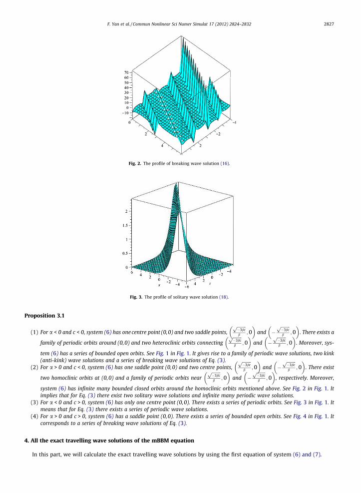
Fig. 2. The profile of breaking wave solution (16).

Fig. 3. The profile of solitary wave solution (18).

F. Yan et al. / Commun Nonlinear Sci Numer Simulat 17 (2012) 2824–2832 2827

Proposition 3.1

(1) For a < 0 and c < 0, system (6) has one centre point (0,0) and two saddle points,ffiffiffiffiffiffiffiffi�3bcp

b ;0� �

and �ffiffiffiffiffiffiffiffi�3bcp

b ;0� �

. There exists a

family of periodic orbits around (0,0) and two heteroclinic orbits connectingffiffiffiffiffiffiffiffi�3bcp

b ;0� �

and �ffiffiffiffiffiffiffiffi�3bcp

b ;0� �

. Moreover, sys-

tem (6) has a series of bounded open orbits. See Fig. 1 in Fig. 1. It gives rise to a family of periodic wave solutions, two kink(anti-kink) wave solutions and a series of breaking wave solutions of Eq. (3).

(2) For a > 0 and c < 0, system (6) has one saddle point (0,0) and two centre points,ffiffiffiffiffiffiffiffi�3bcp

b ;0� �

and �ffiffiffiffiffiffiffiffi�3bcp

b ;0� �

. There exist

two homoclinic orbits at (0,0) and a family of periodic orbits nearffiffiffiffiffiffiffiffi�3bcp

b ; 0� �

and �ffiffiffiffiffiffiffiffi�3bcp

b ;0� �

, respectively. Moreover,

system (6) has infinite many bounded closed orbits around the homoclinic orbits mentioned above. See Fig. 2 in Fig. 1. Itimplies that for Eq. (3) there exist two solitary wave solutions and infinite many periodic wave solutions.

(3) For a < 0 and c > 0, system (6) has only one centre point (0,0). There exists a series of periodic orbits. See Fig. 3 in Fig. 1. Itmeans that for Eq. (3) there exists a series of periodic wave solutions.

(4) For a > 0 and c > 0, system (6) has a saddle point (0,0). There exists a series of bounded open orbits. See Fig. 4 in Fig. 1. Itcorresponds to a series of breaking wave solutions of Eq. (3).

4. All the exact travelling wave solutions of the mBBM equation

In this part, we will calculate the exact travelling wave solutions by using the first equation of system (6) and (7).

Fig. 4. The profile of periodic wave solution (20).

2828 F. Yan et al. / Commun Nonlinear Sci Numer Simulat 17 (2012) 2824–2832

Obviously, by Eq. (7), we get

w2 ¼ 1au2 þ b

6acu4 þ h: ð11Þ

4.1. Case h = 0

By the first equation of system (6), we obtain

n ¼Z

duw¼ �

Zduffiffiffiffiffiffiffiffiffiffiffiffiffiffiffiffiffiffiffiffiffiffiffiffiffiffiffi

1a u2 þ b

6ac u4q : ð12Þ

When a < 0, the following result is hold:

n ¼ �ffiffiffiffiffiffiffi�ap

arctan �ffiffiffi6pffiffiffiffiffiffiffiffiffiffiffiffiffiffiffiffiffiffiffiffi� bu2

c � 6q

0B@

1CA ð13Þ

and when a > 0, the following result is obtained:

n ¼ �ffiffiffiap

ln12þ 2

ffiffiffi6p ffiffiffiffiffiffiffiffiffiffiffiffiffiffiffiffiffiffi

bc u2 þ 6

qau

0@

1A; ð14Þ

where n = x + ct.Taking tan functions on the two sides of (13), the solution of (3) is obtained.

uðx; tÞ ¼ �ffiffiffiffiffiffiffiffiffiffiffiffi�6bc

pb

cscxþ ctffiffiffiffiffiffiffi�ap

� �: ð15Þ

Specially, when a = �1, b = 1, c = �1, we have the following representation of the breaking pattern of (3)

uðx; tÞ ¼ �ffiffiffi6p

cscðx� tÞ: ð16Þ

The profile is shown in Fig. 2. In fact, this breaking pattern corresponds to an open bounded orbit shown in Fig. 1(1).A breaking wave is a wave whose amplitude reaches a critical level at which some process can suddenly start to occur

that causes large amounts of wave energy to be transformed into turbulent kinetic energy. Whitham [24] observed that solu-tions of the KdV equation do not break as physical water waves do, it is intriguing to find mathematical equations for shallowwater waves including the breaking phenomenon. For models describing water waves, we say that wave breaking holds ifthe solution (representing the wave) remains bounded but its slope becomes infinite in finite time: the profile will graduallysteepen as it propagates until it finally develops a point where the slope is vertical and the wave is said to have broken[24].We see that solution (16) present this remarkable property. Therefore, mBBM equation has certain advantages than KdVequation.

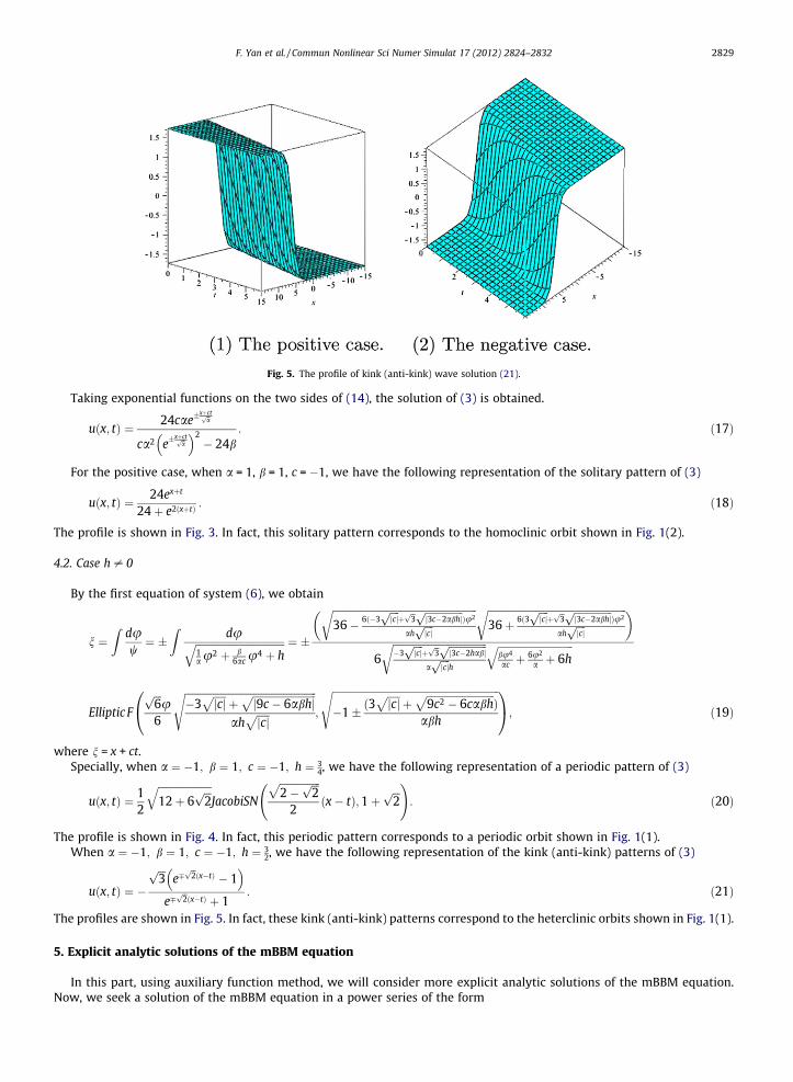
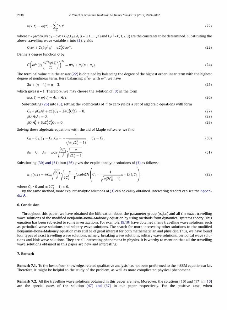
Fig. 5. The profile of kink (anti-kink) wave solution (21).

F. Yan et al. / Commun Nonlinear Sci Numer Simulat 17 (2012) 2824–2832 2829

Taking exponential functions on the two sides of (14), the solution of (3) is obtained.

uðx; tÞ ¼ 24cae�xþctffiffi

ap

ca2 e�xþctffiffi

ap

� �2� 24b

: ð17Þ

For the positive case, when a = 1, b = 1, c = �1, we have the following representation of the solitary pattern of (3)

uðx; tÞ ¼ 24exþt

24þ e2ðxþtÞ : ð18Þ

The profile is shown in Fig. 3. In fact, this solitary pattern corresponds to the homoclinic orbit shown in Fig. 1(2).

4.2. Case h – 0

By the first equation of system (6), we obtain

n ¼Z

duw¼ �

Zduffiffiffiffiffiffiffiffiffiffiffiffiffiffiffiffiffiffiffiffiffiffiffiffiffiffiffiffiffiffiffiffiffiffiffi

1a u2 þ b

6ac u4 þ hq ¼ �

ffiffiffiffiffiffiffiffiffiffiffiffiffiffiffiffiffiffiffiffiffiffiffiffiffiffiffiffiffiffiffiffiffiffiffiffiffiffiffiffiffiffiffiffiffiffiffiffiffiffiffiffiffiffiffiffiffi36� 6ð�3

ffiffiffiffijcjp

þffiffi3p ffiffiffiffiffiffiffiffiffiffiffiffiffiffiffi

j3c�2abhjp

Þu2

ahffiffiffiffijcjp

r ffiffiffiffiffiffiffiffiffiffiffiffiffiffiffiffiffiffiffiffiffiffiffiffiffiffiffiffiffiffiffiffiffiffiffiffiffiffiffiffiffiffiffiffiffiffiffiffiffiffiffiffiffiffiffi36þ 6ð3

ffiffiffiffijcjp

þffiffi3p ffiffiffiffiffiffiffiffiffiffiffiffiffiffiffi

j3c�2abhjp

Þu2

ahffiffiffiffijcjp

r� �

6ffiffiffiffiffiffiffiffiffiffiffiffiffiffiffiffiffiffiffiffiffiffiffiffiffiffiffiffiffiffiffiffiffiffiffiffiffi�3

ffiffiffiffijcjp

þffiffi3p ffiffiffiffiffiffiffiffiffiffiffiffiffiffiffi

j3c�2habjp

affiffiffiffijcjp

h

r ffiffiffiffiffiffiffiffiffiffiffiffiffiffiffiffiffiffiffiffiffiffiffiffiffiffiffiffiffiffibu4

ac þ6u2

a þ 6hq

Elliptic F

ffiffiffi6p

u6

ffiffiffiffiffiffiffiffiffiffiffiffiffiffiffiffiffiffiffiffiffiffiffiffiffiffiffiffiffiffiffiffiffiffiffiffiffiffiffiffiffiffiffiffiffiffiffiffiffiffiffiffi�3

ffiffiffiffiffijcj

pþ

ffiffiffiffiffiffiffiffiffiffiffiffiffiffiffiffiffiffiffiffiffiffiffiffiffij9c � 6abhj

pah

ffiffiffiffiffijcj

ps

;

ffiffiffiffiffiffiffiffiffiffiffiffiffiffiffiffiffiffiffiffiffiffiffiffiffiffiffiffiffiffiffiffiffiffiffiffiffiffiffiffiffiffiffiffiffiffiffiffiffiffiffiffiffiffiffiffiffiffiffiffiffiffiffiffiffiffi�1� ð3

ffiffiffiffiffijcj

pþ

ffiffiffiffiffiffiffiffiffiffiffiffiffiffiffiffiffiffiffiffiffiffiffiffiffiffiffi9c2 � 6cabh

pÞ

abh

s0@

1A; ð19Þ

where n = x + ct.Specially, when a ¼ �1; b ¼ 1; c ¼ �1; h ¼ 3

4, we have the following representation of a periodic pattern of (3)

uðx; tÞ ¼ 12

ffiffiffiffiffiffiffiffiffiffiffiffiffiffiffiffiffiffiffiffiffi12þ 6

ffiffiffi2pq

JacobiSN

ffiffiffiffiffiffiffiffiffiffiffiffiffiffiffiffi2�

ffiffiffi2pp

2ðx� tÞ;1þ

ffiffiffi2p

!: ð20Þ

The profile is shown in Fig. 4. In fact, this periodic pattern corresponds to a periodic orbit shown in Fig. 1(1).When a ¼ �1; b ¼ 1; c ¼ �1; h ¼ 3

2, we have the following representation of the kink (anti-kink) patterns of (3)

uðx; tÞ ¼ �

ffiffiffi3p

e�ffiffi2pðx�tÞ � 1

� �e�ffiffi2pðx�tÞ þ 1

: ð21Þ

The profiles are shown in Fig. 5. In fact, these kink (anti-kink) patterns correspond to the heterclinic orbits shown in Fig. 1(1).

5. Explicit analytic solutions of the mBBM equation

In this part, using auxiliary function method, we will consider more explicit analytic solutions of the mBBM equation.Now, we seek a solution of the mBBM equation in a power series of the form

2830 F. Yan et al. / Commun Nonlinear Sci Numer Simulat 17 (2012) 2824–2832

uðx; tÞ ¼ uðsÞ ¼Xn

i¼0

Aisi; ð22Þ

where s = JacobiCN (C1 + C2x + C3t,C0), Ai (i = 0,1, . . . ,n) and Ci (i = 0,1,2,3) are the constants to be determined. Substituting theabove travelling wave variable s into (3), yields

C3u0 þ C2bu2u0 � aC22C3u000: ð23Þ

Define a degree function G by

G ua1 ðnÞ da2uðnÞdn

� �� �a3

¼ na1 þ a3ðnþ a2Þ: ð24Þ

The terminal value n in the ansatz (22) is obtained by balancing the degree of the highest order linear term with the highestdegree of nonlinear term. Here balancing u2u0 with u000, we have

2nþ ðnþ 1Þ ¼ nþ 3; ð25Þ

which gives n = 1. Therefore, we may choose the solution of (3) in the form

uðx; tÞ ¼ uðsÞ ¼ A0 þ A1s: ð26Þ

Substituting (26) into (3), setting the coefficients of si to zero yields a set of algebraic equations with form

C3 þ bC2A20 þ aC2

2C3 � 2aC20C2

2C3 ¼ 0; ð27ÞbC2A0A1 ¼ 0; ð28ÞbC2A2

1 þ 6aC20C2

2C3 ¼ 0: ð29Þ

Solving these algebraic equations with the aid of Maple software, we find

C0 ¼ C0;C1 ¼ C1;C2 ¼ �1ffiffiffiffiffiffiffiffiffiffiffiffiffiffiffiffiffiffiffiffiffiffiffiffi

að2C20 � 1Þ

q ; C3 ¼ C3; ð30Þ

A0 ¼ 0; A1 ¼ �C0

ffiffiffiffiffiffiffiffi6C3

b

s ffiffiffiffiffiffiffiffiffiffiffiffiffiffiffiffiffia

2C20 � 1

4

s: ð31Þ

Substituting (30) and (31) into (26) gives the explicit analytic solutions of (3) as follows:

u1;2ðx; tÞ ¼ �C0

ffiffiffiffiffiffiffiffi6C3

b

s ffiffiffiffiffiffiffiffiffiffiffiffiffiffiffiffiffia

2C20 � 1

4

sJacobiCN C1 �

1ffiffiffiffiffiffiffiffiffiffiffiffiffiffiffiffiffiffiffiffiffiffiffiffiað2C2

0 � 1Þq xþ C3t;C0

0B@

1CA; ð32Þ

where C3 > 0 and að2C20 � 1Þ > 0.

By the same method, more explicit analytic solutions of (3) can be easily obtained. Interesting readers can see the Appen-dix A.

6. Conclusion

Throughout this paper, we have obtained the bifurcation about the parameter group (a,b,c) and all the exact travellingwave solutions of the modified Benjamin–Bona–Mahoney equation by using methods from dynamical systems theory. Thisequation has been subjected to some investigations. For example, [9,10] have obtained many travelling wave solutions suchas periodical wave solutions and solitary wave solutions. The search for more interesting other solutions to the modifiedBenjamin–Bona–Mahoney equation may still be of great interest for both mathematician and physicist. Thus, we have foundfour types of exact travelling wave solutions, namely, breaking wave solutions, solitary wave solutions, periodical wave solu-tions and kink wave solutions. They are all interesting phenomena in physics. It is worthy to mention that all the travellingwave solutions obtained in this paper are new and interesting.

7. Remark

Remark 7.1. To the best of our knowledge, related qualitative analysis has not been preformed to the mBBM equation so far.Therefore, it might be helpful to the study of the problem, as well as more complicated physical phenomena.

Remark 7.2. All the travelling wave solutions obtained in this paper are new. Moreover, the solutions (16) and (17) in [10]are the special cases of the solution (47) and (37) in our paper respectively. For the positive case, when

F. Yan et al. / Commun Nonlinear Sci Numer Simulat 17 (2012) 2824–2832 2831

C1 ¼ 12

ffiffiffiffiffiffiffiffiffiffiffiffiffiffiffiffiffiffiffiffiffiffiffiffiffiffiffiffiffiffi�a2 þ b2 � c2

px; C3 ¼ 1

6bkA2

0ð�a2þb2�c2Þ32

c2 ; a ¼ 2�a2þb2�c2, the solution (47) in our paper is the same as the solution (16) in

[10]. When we take C1 ¼ 12

ffiffiffiffiffiffiffiffiffiffiffiffiffiffiffiffiffiffiffiffiffiffiffiffiffiffia2 � b2 þ c2

px; C3 ¼ � 1

6bkA2

0ða2�b2þc2Þ32

c2 ; a ¼ 2�a2þb2�c2, the solution (37) in our paper is the same as

the solution (17) in [10].

Acknowledgements

The authors express their gratitude to the anonymous referees for their helpful suggestions and the partial support ofNSFC (10832006/11172158) and Yunnan NSFC (2011FZ086).

Appendix A

Using auxiliary function method, several types of explicit analytic solutions of the mBBM equation are obtained asfollowings:

u1;2ðx; tÞ ¼ �

ffiffiffiffiffiffiffiffi6C3

b

s ffiffiffiffiffiffiffiffiffiffiffiffiffiffiffiffiffiffiffiffiffiffiffiffiffia C2

0 � 1� �2

2C20 � 1

4

vuuut JacobiNC C1 þ1ffiffiffiffiffiffiffiffiffiffiffiffiffiffiffiffiffiffiffiffiffiffiffiffi

að2C20 � 1Þ

q xþ C3t;C0

0B@

1CA; C3 > 0; a 2C2

0 � 1� �

> 0; kC0j < 1; ð33Þ

u3;4ðx; tÞ ¼ �

ffiffiffiffiffiffiffiffi6C3

b

s ffiffiffiffiffiffiffiffiffiffiffiffiffiffiffiffiffiffiffiffiffiffiffiffiffia C2

0 � 1� �2

2C20 � 1

4

vuuut JacobiNC C1 �1ffiffiffiffiffiffiffiffiffiffiffiffiffiffiffiffiffiffiffiffiffiffiffiffiffiffi

a 2C20 � 1

� �r xþ C3t;C0

0BB@

1CCA; C3 > 0; a 2C2

0 � 1� �

> 0; kC0j > 1; ð34Þ

u5;6ðx; tÞ ¼ �

ffiffiffiffiffiffiffiffiffiffiffiffiffiffiffiffiffiffiffiffiffiffi�3C3

ffiffiffiffiffiffi2ap

b

scot C1 �

1ffiffiffiffiffiffi2ap xþ C3t

� �; a > 0; C3 < 0; ð35Þ

u7;8ðx; tÞ ¼ �

ffiffiffiffiffiffiffiffiffiffiffiffiffiffiffiffiffiffi3C3

ffiffiffiffiffiffi2ap

b

scot C1 þ

1ffiffiffiffiffiffi2ap xþ C3t

� �; a > 0; C3 > 0; ð36Þ

u9;10ðx; tÞ ¼ �

ffiffiffiffiffiffiffiffiffiffiffiffiffiffiffiffiffiffiffiffiffiffi3C3

ffiffiffiffiffiffiffiffiffiffi�2ap

b

scoth C1 �

1ffiffiffiffiffiffiffiffiffiffi�2ap xþ C3t

� �; a < 0; C3 > 0; ð37Þ

u11;12ðx; tÞ ¼ �

ffiffiffiffiffiffiffiffiffiffiffiffiffiffiffiffiffiffiffiffiffiffiffiffiffi�3C3

ffiffiffiffiffiffiffiffiffiffi�2ap

b

scoth C1 þ

1ffiffiffiffiffiffiffiffiffiffi�2ap xþ C3t

� �; a < 0; C3 < 0; ð38Þ

u13;14ðx; tÞ ¼ �

ffiffiffiffiffiffiffiffiffiffiffiffiffiffiffiffiffiffiffi6C3

ffiffiffiffiffiffiffi�ap

b

scsc C1 �

1ffiffiffiffiffiffiffi�ap xþ C3t

� �; a < 0; C3 > 0; ð39Þ

u15;16ðx; tÞ ¼ �

ffiffiffiffiffiffiffiffiffiffiffiffiffiffiffiffiffiffiffiffiffiffiffi�6C3

ffiffiffiffiffiffiffi�ap

b

scsc C1 þ

1ffiffiffiffiffiffiffi�ap xþ C3t

� �; a < 0; C3 < 0; ð40Þ

u17;18ðx; tÞ ¼ �

ffiffiffiffiffiffiffiffiffiffiffiffiffiffiffiffiffiffiffi�6C3

ffiffiffiap

b

scsch C1 �

1ffiffiffiap xþ C3t

� �; a > 0; C3 < 0; ð41Þ

u19;20ðx; tÞ ¼ �

ffiffiffiffiffiffiffiffiffiffiffiffiffiffiffi6C3

ffiffiffiap

b

scsch C1 þ

1ffiffiffiap xþ C3t

� �; a > 0; C3 > 0; ð42Þ

u21;22ðx; tÞ ¼ �

ffiffiffiffiffiffiffiffiffiffiffiffiffiffiffiffiffiffiffi6C3

ffiffiffiffiffiffiffi�ap

b

ssec C1 �

1ffiffiffiffiffiffiffi�ap xþ C3t

� �; a < 0; C3 > 0; ð43Þ

u23;24ðx; tÞ ¼ �

ffiffiffiffiffiffiffiffiffiffiffiffiffiffiffiffiffiffiffiffiffiffiffi�6C3

ffiffiffiffiffiffiffi�ap

b

ssec C1 þ

1ffiffiffiffiffiffiffi�ap xþ C3t

� �; a < 0; C3 < 0; ð44Þ

u25;26ðx; tÞ ¼ �

ffiffiffiffiffiffiffiffiffiffiffiffiffiffiffiffiffiffiffi�6C3

ffiffiffiap

b

ssech C1 þ

1ffiffiffiap xþ C3t

� �; a > 0; C3 < 0; ð45Þ

u27;28ðx; tÞ ¼ �

ffiffiffiffiffiffiffiffiffiffiffiffiffiffiffi6C3

ffiffiffiap

b

ssech C1 �

1ffiffiffiap xþ C3t

� �; a > 0; C3 > 0; ð46Þ

2832 F. Yan et al. / Commun Nonlinear Sci Numer Simulat 17 (2012) 2824–2832

u29;30ðx; tÞ ¼ �

ffiffiffiffiffiffiffiffiffiffiffiffiffiffiffiffiffiffiffiffiffiffi�3C3

ffiffiffiffiffiffi2ap

b

stan C1 �

1ffiffiffiffiffiffi2ap xþ C3t

� �; a > 0; C3 < 0; ð47Þ

u31;32ðx; tÞ ¼ �

ffiffiffiffiffiffiffiffiffiffiffiffiffiffiffiffiffiffi3C3

ffiffiffiffiffiffi2ap

b

stan C1 þ

1ffiffiffiffiffiffi2ap xþ C3t

� �; a > 0; C3 > 0; ð48Þ

u33;34ðx; tÞ ¼ �

ffiffiffiffiffiffiffiffiffiffiffiffiffiffiffiffiffiffiffiffiffiffi3C3

ffiffiffiffiffiffiffiffiffiffi�2ap

b

stanh C1 �

1ffiffiffiffiffiffiffiffiffiffi�2ap xþ C3t

� �; a < 0; C3 > 0; ð49Þ

u35;36ðx; tÞ ¼ �

ffiffiffiffiffiffiffiffiffiffiffiffiffiffiffiffiffiffiffiffiffiffiffiffiffi�3C3

ffiffiffiffiffiffiffiffiffiffi�2ap

b

stanh C1 þ

1ffiffiffiffiffiffiffiffiffiffi�2ap xþ C3t

� �; a < 0; C3 < 0: ð50Þ

References

[1] Korteweg DJ, Vries G de. On the change of form of long waves advancing in a rectangular canal and on a new type of long stationary waves. Philos Mag1895;39:422–43.

[2] Drazin PG, Johnson RS. Soliton: an introduction. Cambridge, UK: Cambridge University Press; 1989.[3] Benjamin TB, Bona JL, Mahony JJ. Model equations for long waves in nonlinear dispersive systems. Philos Trans R Soc Lond Ser A 1972;272:47–78.[4] Biswas A, Konar S. Soliton perturbation theory for the generalized Benjamin–Bona–Mahoney equation. Commun Nonlinear Sci Numer Simulat

2008;13:703–6.[5] Biswas A. Solitary waves for power-law regularized long-wave equation and R(m,n) equation. Nonlinear Dyn 2010;59:423–6.[6] Biswas A. 1-Soliton solution of Benjamin–Bona–Mahoney equation with dual-power law nonlinearity. Commun Nonlinear Sci Numer Simulat

2010;15:2744–6.[7] Wazwaz AM, Helal MA. Nonlinear variants of the BBM equation with compact and noncompact physical structures. Chaos Soliton Fract

2005;26:767–76.[8] Nickel J. Elliptic solutions to a generalized BBM equation. Phys Lett A 2007;364:221–6.[9] Wang JM, Zhang M, Zhang WL, Zhang R, Hua J. A new method for constructing travelling wave solutions to the modified Benjamin–Bona–Mahoney

equation. Chin Phys Lett 2008;25(7):2339–41.[10] Layeni OP, Akinola AP. A new hyperbolic auxiliary function method and exact solutions of the mBBM equation. Commun Nonlinear Sci Numer Simulat

2010;15:133–8.[11] Xu GQ, Li ZB. Exact travelling wave solutions of the Whitham–Broer–Kaup and Broer–Kaup–Kupershmidt equations. Chaos Soliton Fract

2005;24:549–56.[12] El-Wakil SA, Abdou MA, Elhanbaly A. New solitons and periodic wave solutions for nonlinear evolution equations. Phys Lett A 2006;353:40–7.[13] Li X, Wang M. A sub-ODE method for finding exact solutions of a generalized KdV–mKdV equation with high-order nonlinear terms. Phys Lett A

2007;361:115–8.[14] Quan XD. Symmetry reduction and new non-travelling wave solutions of (2+1)-dimensional breaking soliton equation. Commun Nonlinear Sci Numer

Simulat 2010;15:2061–5.[15] Xu LP, Zhang JL. Exact solutions to two higher order nonlinear Schrödinger equations. Chaos Soliton Fract 2007;31:937–42.[16] Zayed EME, Zedan HA, Gepreel KA. On the solitary wave solutions for nonlinear Hirota–Satsuma coupled KdV of equations. Chaos Soliton Fract

2004;22:285–303.[17] Wazwaz AM. Analytic study for fifth-order KdV-type equations with arbitrary power nonlinearities. Commun Nonlinear Sci Numer Simulat

2007;12:904–9.[18] Malfliet W. The tanh method: a tool for solving certain classes of nonlinear evolution and wave equations. J Comput Appl Math 2004;164–165:529–41.[19] Malfliet W, Hereman W. The tanh method: I. Exact solutions of nonlinear evolution and wave equations. Phys Scr 1996;54:563–8.[20] Malfliet W, Hereman W. The tanh method: II. Perturbation technique for conservative systems. Phys Scr 1996;54:569–75.[21] Bian CQ, Pang J, Jin LG, Ying XM. Solving two fifth order strong nonlinear evolution equations by using the G0

G

� �-expansion method. Commun Nonlinear

Sci Numer Simulat 2010;15:2337–43.[22] Wazwaz AM. Multiple-soliton solutions of the perturbed KdV equation. Commun Nonlinear Sci Numer Simulat 2010;15:3270–3.[23] Shang YD, Huang Y. The Bäcklund transformations and abundant explicit exact solutions for the AkNS–SWWW equation. Commun Nonlinear Sci

Numer Simulat 2011;16:2445–55.[24] Whitham GB. Linear and nonlinear waves. New York: Wiley; 1974.