The Biases of Others: Anticipating Informational

Projection in an Agency Setting∗

David N. Danz†, Kristof Madarasz‡, Stephanie W. Wang§

November 9, 2017

Abstract

Evidence shows that people fail to account for informational differ-ences and instead project their information onto others in that they toooften act as if others had access to the same information they did. Inthis study, we find that while people naively project their informationonto others, they also anticipate the projection of their differentiallyinformed opponents onto them. Specifically, we directly test the modelof projection equilibrium, Madarasz (2014), a single-parameter exten-sion of common prior BNE which posits a tight continuous relationshipbetween the extent to which people project onto others and the extentto which they anticipate the projection of others onto them. Consis-tent with the theory, we find not only that on average better-informedprincipals exaggerate the extent to which lesser informed agents shouldact as if they were better-informed, but that on average lesser-informedagents anticipate but underestimate such misperceptions as revealed bytheir choice of incentive scheme and elicited second-order beliefs. Fur-thermore, we estimate the distribution of the extent to which playersproject onto others and the distribution of the extent to which players

∗We are grateful for valuable comments by Colin Camerer, Gary Charness, John Duffy,Ignacio Esponda, Dorothea Kubler, Muriel Niederle, Demian Pouzo, Andrew Schotter,Adam Szeidl, Lise Vesterlund, Axel Werwatz, and Alistair Wilson. Financial supportfrom the Deutsche Forschungsgemeinschaft (DFG) through CRC 649 “Economic Risk” isgratefully acknowledged.†University of Pittsburgh, 4924 Wesley W. Posvar Hall, 230 South Bouquet Street,

Pittsburgh, PA 15260 and WZB Berlin Social Science Center, danz@pitt.edu.‡London School of Economics and Political Science, WC2A 2AE, UK,

k.p.madarasz@lse.ac.uk.§University of Pittsburgh, 4715 Wesley W. Posvar Hall, 230 South Bouquet Street,

Pittsburgh, PA 15260, swwang@pitt.edu.

1

fail to recognize others’ projection onto them and find that the rela-tionship between the two is remarkably consistent with that impliedby projection equilibrium.

Keywords: information projection, defensive agency, curse of knowledge,hindsight bias, higher-order beliefs

1 Introduction

Over the past decades significant effort has been devoted to documentingdomains where a person’s choice departs from classical notions of rationality.At the same time, less attention has been devoted to the issue of understand-ing the extent to which people anticipate such departures, in particular, littleis known about whether people anticipate or mispredict such departures inothers. In the context of an individual bias, one’s own departure from ra-tionality can be studied separately from one’s anticipation of the same kindof departure by others. In the context of a general social bias, as consideredby this paper, where the failure of rationality lies in a person’s belief aboutthe beliefs of others, such a separation need not be possible.

In particular, this paper considers the essential psychological domain ofthe theory of mind, e.g., Piaget (1956), that is, the way people form be-liefs about the beliefs of others. The phenomenon of informational projec-tion (Madarasz 2012, 2016) formalizes a general shortcoming in this domainwhereby people engage in limited perspective taking and act as if they at-tributed information to others that are too close to their own. For example,a theory teacher who exhibits the curse-of-knowledge and exaggerates theamount of background knowledge her students have tends to explain thematerial in terms that are too complex for her students to understand.

In many economically relevant situations what matters is not simplywhat beliefs a person has about the information of others, but also what shethinks about others’ think her beliefs and information is. In other words,specifying such second-order perceptions is key. A poker player may exag-gerate the extent to which others know her hand, but does she also thinkthat others wrongly assume that she might know their hands? A game the-ory teacher who exhibits the curse of knowledge too often thinks that herstudents should already know what a Nash equilibrium is. Does she, how-ever, anticipate that her students too often expect her to know that theyhave very little idea about Nash equilibrium? Will this not directly contra-dict the first-order implications of the curse-of-knowledge? In all these, and

2

many other settings, specifying the extent to which one anticipates the mis-takes of others becomes part of the very definition of one’s own mistake. Ina social context, studying empirically the extent to which people anticipateeach other’s biases is essential to study the nature and the form of the biasitself.

Answering the question whether or not people anticipate the biases ofothers is important not only to provide a coherent and empirically plausi-ble account of projection per se, but has directly relevant implications fora variety of economic outcomes. For example, in the fundamental agencyproblem characterizing organizations, if an agent anticipates that monitor-ing with ex-post information will bias a principal’s assessment of her andadversely affect her reputation, she may try to manipulate the productionof ex-ante information or simply dis-invest from an otherwise efficient re-lationship. Thus, classical tools that could reduce agency costs under theassumption of no such anticipation could offer perverse incentives and in-stead exacerbate inefficiencies.

A widely discussed example of such defensive agency can be found in thecontext of medical malpractice liability. The radiologist Leonard Berlin, inhis 2003 testimony on the regulation of mammography to the U.S. SenateCommittee on Health, Education, Labor, and Pensions, describes how ex-post information causes the public to misperceive the ex-ante accuracy ofmammograms, implying that juries are “all too ready to grant great compen-sation.” Berlin references the role of information projection in such ex-postassessments, where ex-post information makes reading old radiographs mucheasier.1 In response, physicians are reluctant to follow such crucial diagnosticpractices: “The end result is that more and more radiologists are refusing toperform mammography [...] In turn, mammography facilities are closing.”

In the context of such systematic false beliefs that do not follow thetenants of common priors standard strategic models provide no particularguidance. A direct and simple response to the presence of higher-order con-siderations in contexts where projection may be key is to assume a binaryclassification of people into biased ones who also fail to anticipate the biasesof others and unbiased ones who, in contrast, do anticipate the biases of oth-ers. While this still naive classification is still under-specified as it leaves keyhigher-order considerations open, e.g., a player’s belief about her opponent’sbelief of her degree of projection, it resolves the apparent contradiction be-

1As Berlin (2003) points out “Suffice it to say that research studies performed at someof the most prestigious medical institutions of the United States reveal that as many as90% of lung cancers and 70% of breast cancers can at least be partially observed on studiespreviously read as normal.”

3

tween projecting information and anticipating the projection of others andmay also prove to be a useful first approximation. In another vein, one mayalso suppose that the extent to which the average person project onto othersin a context provides no prediction as to the average person’s anticipationof others’ projection in that context.

In contrast, the model of Madarasz (2014) offers a more continuous andfully specified equilibrium approach, projection equilibrium. This admits thebehavioral types of the above binary specifications as two limiting extremes.This model provides a general and fully specified approach. At the sametime, by tying together the extent to which people project their informationonto others (first-order projection) and the extent to which they fail to an-ticipate others’ projecting onto them (second-order projection), it provides astill very parsimonious alternative. It offers a single-parameter extension ofthe common-prior Bayesian Nash Equilibrium and implies a measure underwhich the extent to which people are biased is directly and inversely relatedto the extent to which they anticipate the biases of others. Specifically, un-der the model of projection equilibrium, a person who projects to degree ρacts as if she (wrongly) believed that her opponent knew exactly her infor-mation, had correct beliefs about her beliefs about his information and so onwith probability ρ and, with the remaining probability 1−ρ, she has correctbeliefs about her opponent’s information, correct beliefs about her oppo-nent’s (wrong) beliefs about her information and so on. A tight implicationof the model is that if a person acts as if she mistakenly believed that othersknew her information with probability ρ, first-order projection, she also actsas if she underestimated the analogous beliefs of others by probability ρ2,second-order projection. It predicts that the extent to which people projectonto others is inversely related to the square-root of the extent to whichthey fail to anticipate how much others project onto them. The extent towhich this single-parameter model provides greater explanatory power thana more naive alternative is ultimately an empirical question.

This paper develops a simple experimental design to directly test thistheory. Moreover, the design not only allows one to test the equilibriummodel against the perfect Bayesian equilibrium with correct priors, but isable to assess the relevance of the continuous specification over a more naivedichotomous classification of people into biased (unanticipating) and unbi-ased (fully anticipating) types. In addition, it is also able to tightly describethe extent to which a single-parameter parsimonious specification which di-rectly links the first-order and the second-order mistake is able to capturekey aspects of the data.

4

In our experiments, principals (evaluators) estimated the average per-formance of agents in a real-effort task. The principals received the solutionto each task prior to the estimation in the informed treatment but not inthe uninformed (control) treatment. Agents are randomly matched witheither informed or uninformed principals depending on the treatment. Ifa principal exaggerates the extent to which agents act as if they had thesame information as she did, then on average a principal in the informed,but not in the uninformed treatment, should overestimate the agents’ per-formance. The difference between the principals’ performance estimationsin the treatment vs. control then allows us to identify the extent of theprincipals’ information projection in first-order beliefs. We do find strongevidence of first-order informational projection by principals in our experi-ments, consistent with previous results.

For each task, the agents could choose between a sure payoff and aninvestment whose payoff was decreasing in the principal’s expectation of thesuccess rate in the task. If the agents anticipate that informed principalsoverestimate their performance on average, vis-a-vis the estimates in thecontrol treatment, then they would prefer the sure payoff, which is not de-pendent upon the principals’ estimation, more in the informed than in theuninformed treatment. We find that 67.3% of agents matched with informedprincipals as opposed to 39.2% of those matched with uninformed principalschose the investment whose payoff was decreasing in the principal’s estima-tion.

To further explore the issue of anticipation in beliefs, we also directlyelicited the agents’ both first-order (their own estimate of the success rate)and second-order beliefs (their estimate of the principals’ estimates of thesuccess rate). Indeed, we find clear evidence that agents anticipate thatprincipals are biased by private information. In particular, agents’ first-order beliefs are well-calibrated on average in both treatments. Further-more, agents’ second-order beliefs do not differ from their first-order beliefsin the uninformed treatment, at the same time, their second-order beliefsare significantly higher than their own first-order beliefs in the informedtreatment. These findings lend direct support to projection equilibrium.

We then use the estimates by informed principals and the first- andsecond-order beliefs of agents matched to informed principals to estimateprojection equilibrium, which nests the Bayesian Nash equilibrium as a spe-cial case. Under projection equilibrium, a person simultaneously projectsonto others, and to a lesser extent—where this lesser extent is also governedby projection itself—she anticipates others will project onto her. The factthat such anticipation under projection is limited stems from the fact that

5

a person who projects too often thinks others not only have the same basicperspective as she does, but also a truthful perspective (second-order belief)about her perspective as well. Consistent with the predictions of projectionequilibrium, we find the exaggeration anticipated by the agents matchedwith informed principals is positive—but, as the model predicts, less thanthe actual exaggeration exhibited by the informed principals. We estimatethe single-parameter version of projection equilibrium and find significantinformation projection. Crucially, we then relax the assumption that theprincipal and the agent must exhibit the same degree of projection, that is,that the degree to which people project their information on others is thesquare-root of the extent to which people underestimate others’ projectiononto them, and nevertheless obtain very similar parameter estimates andlog-likelihoods. Finally, we also compare the distribution of first-order pro-jection in the population and the distribution of the under-anticipation, thatis, the extent to which agents underestimate the principal’s overestimation.We find that these two distributions are remarkably close to each other.

The paper is structured as follows. In Section 2, we present the exper-imental design and procedures. Section 3 enumerates the model and themain predictions. Section 4 contains the results. In Section 5, we concludewith a discussion of related models and future directions.

2 Experimental Design

2.1 Experimental task

All participants worked on the same series of 20 information-projection stim-uli: In each of 20 change-detection tasks, the subjects had to find the dif-ference between two otherwise identical images (see Rensink et al., 1997;Simons and Levin, 1997). Figure 1 shows an example, where the differenceis located in the upper-right corner of the images. While the difference be-tween these images is quite hard to detect, it seems obvious once you knowwhere to look. In turn, people who know the solution in the first place,cannot “unsee” it and hence tend to overestimate how likely others will findit (see, e.g., Loewenstein et al. 2006).2

We presented each task in a 14-second video clip in which the two imageswere displayed alternately with short interruptions.3 Afterwards, subjects

2Further information-projection stimuli typically used in experiments are predictiontasks (in various contexts), logic puzzles, and trivia questions.

3Each image was displayed for one second, followed by a blank screen for 150 millisec-onds.

6

Image A Image B

Figure 1: Example of an image pair. Image sequence in the experiment: A,B, A, B, . . . .

had 40 seconds to submit an answer, i.e., to indicate the location of thedifference.4

2.2 Principals

Principals had to estimate the performance of others in the change-detectiontasks. Specifically, the principals were told that subjects in previous sessionsworked on the tasks and that these subjects (reference agents henceforth)were paid according to their performance.5

In each of 20 rounds, the principals were first exposed to the task; thatis, they watched the 14-second video clip and then had 40 seconds to submita solution to the task. Afterwards, the principals stated their belief (bPt )about the fraction of reference agents who spotted the difference in thattask (success rate πt henceforth). After each principal stated his or herbelief, the next round started.6

For the principals the two treatments differed as follows. In the informedtreatment, the principals received the solution to each task before they wentthrough the change-detection task. Specifically, during a countdown phasethat announced the start of each task, the screen showed the image (oneof the two in the video) with the difference highlighted with a red circle(see Figure 2). In the uninformed treatment, the principals were not given

4See the instructions in the Appendix for more details.5The performance data of 144 reference agents was taken from Danz (2014). In their

experiment, the subjects performed the tasks in winner-take-all tournaments, where theyfaced the tasks in exactly the same way as the subjects in the current experiment.

6The principals first participated in three practice rounds to become familiar with theinterface.

7

solutions to the tasks (the same image was shown on the countdown screen,but without the red circle and the note). Principals in both treatments thenwent through each task exactly as the reference agents did. The principalsdid not receive feedback of any kind during the experiment.

Task 1 of 20 starts in [sec]: 6

Note: The difference is located in the red marked area (the previous performers did not receive a solution guide).

Remaining time [sec]: 61

Figure 2: Screenshot from the treatment with informed principals: Count-down to the next task providing the solution (translated from German).

At the end of the sessions, the principals received e 0.50 for each correctanswer in the uninformed treatment and e 0.30 in the informed treatment.In addition, they were paid based on the accuracy of their stated beliefs intwo of the 20 tasks (randomly chosen): for each of these two tasks, theyreceived e 12 if bPt ∈ [πt−0.05, πt+ 0.05], that is, if the estimate was within5 percentage points of the true success rate of the agents. We ran onesession with informed principals, and one with uninformed principals with24 participants in each.

2.3 Agents

Agents in both treatments were informed that in previous sessions (i) refer-ence agents had performed the change-detection tasks being paid accordingto their performance and (ii) principals had estimated the average perfor-mance of the reference agents being paid according to the accuracy of theirestimates. The agents where further told that they had been randomlymatched to one of the principals at the outset of the experiment and thatthis matching would remain the same for the duration of the experiment.For the agents, the two treatments differed only with respect to the kind

8

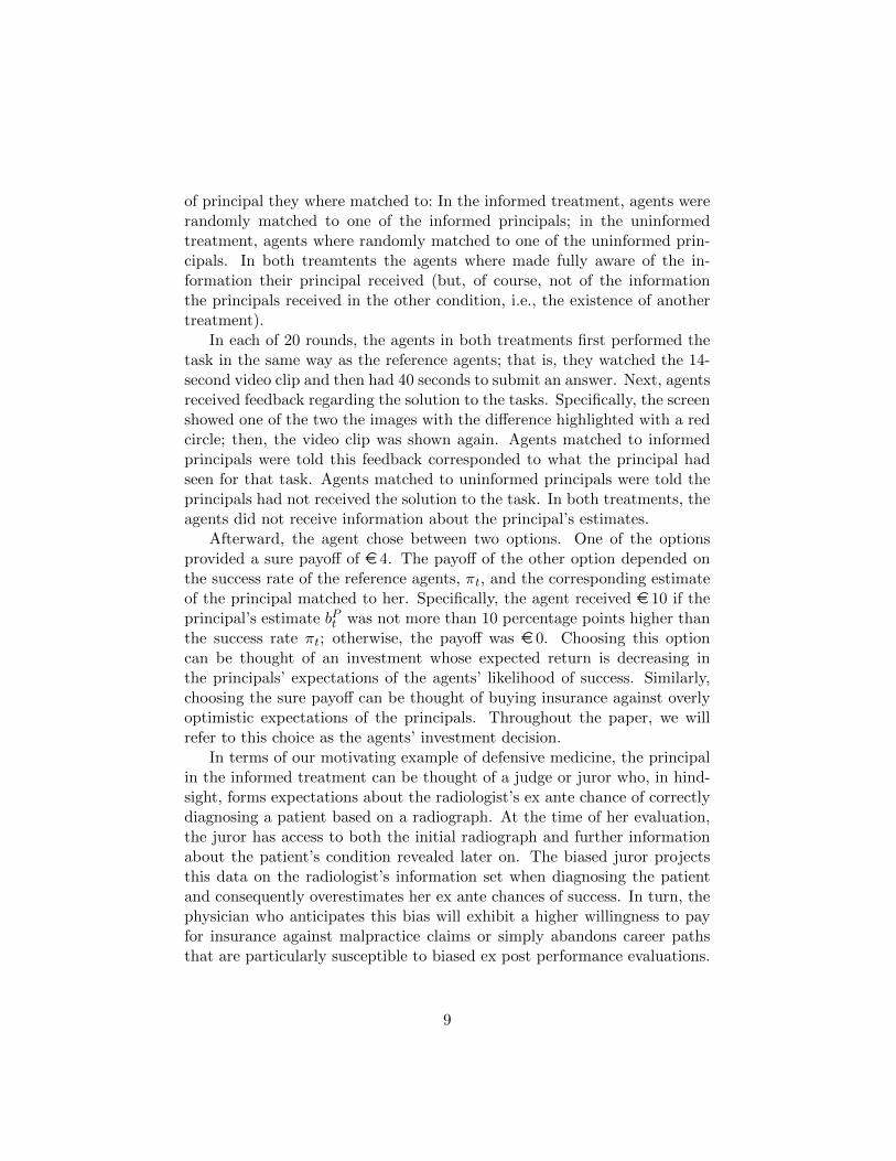
of principal they where matched to: In the informed treatment, agents wererandomly matched to one of the informed principals; in the uninformedtreatment, agents where randomly matched to one of the uninformed prin-cipals. In both treamtents the agents where made fully aware of the in-formation their principal received (but, of course, not of the informationthe principals received in the other condition, i.e., the existence of anothertreatment).

In each of 20 rounds, the agents in both treatments first performed thetask in the same way as the reference agents; that is, they watched the 14-second video clip and then had 40 seconds to submit an answer. Next, agentsreceived feedback regarding the solution to the tasks. Specifically, the screenshowed one of the two the images with the difference highlighted with a redcircle; then, the video clip was shown again. Agents matched to informedprincipals were told this feedback corresponded to what the principal hadseen for that task. Agents matched to uninformed principals were told theprincipals had not received the solution to the task. In both treatments, theagents did not receive information about the principal’s estimates.

Afterward, the agent chose between two options. One of the optionsprovided a sure payoff of e 4. The payoff of the other option depended onthe success rate of the reference agents, πt, and the corresponding estimateof the principal matched to her. Specifically, the agent received e 10 if theprincipal’s estimate bPt was not more than 10 percentage points higher thanthe success rate πt; otherwise, the payoff was e 0. Choosing this optioncan be thought of an investment whose expected return is decreasing inthe principals’ expectations of the agents’ likelihood of success. Similarly,choosing the sure payoff can be thought of buying insurance against overlyoptimistic expectations of the principals. Throughout the paper, we willrefer to this choice as the agents’ investment decision.

In terms of our motivating example of defensive medicine, the principalin the informed treatment can be thought of a judge or juror who, in hind-sight, forms expectations about the radiologist’s ex ante chance of correctlydiagnosing a patient based on a radiograph. At the time of her evaluation,the juror has access to both the initial radiograph and further informationabout the patient’s condition revealed later on. The biased juror projectsthis data on the radiologist’s information set when diagnosing the patientand consequently overestimates her ex ante chances of success. In turn, thephysician who anticipates this bias will exhibit a higher willingness to payfor insurance against malpractice claims or simply abandons career pathsthat are particularly susceptible to biased ex post performance evaluations.

9

The agents received e 0.50 for each correct answer to the change-detection tasks. In addition they were also paid according to the outcomeof one randomly selected investment decision. We ran two sessions of agentsmatched to informed principals (24 participants per session) and two sessionwith agents matched to uninformed principals (23 participants per session).

To explore the agents’ beliefs that underlie their investment decisions,we ran additional sessions: one with agents matched to informed principals(24 participants) and one with agents matched to uninformed principals(23 participants). The sessions differed from the sessions without beliefelicitation in that belief elicitation replaced the investment decisions for thefirst ten tasks of the experiment. Specifically, following each of the first 10change-detection tasks (and the feedback regarding the solution), the agentsstated (i) their belief about the fraction of reference agents that spotted thedifference in that task (first-order belief bA1,t henceforth) and (ii) their belief

about their principal’s estimate of that success rate (second-order belief bA2,thenceforth).

At the end of the experiment one round was randomly selected for pay-ment. If this round involved belief elicitation, we randomly selected one ofthe agent’s stated beliefs for payment, namely, either her first- or second-order belief in that round.7 The subject received e 12 if her stated belief waswithin five percentage points of the actual value (the actual success rate incase of a first-order belief and the principal’s estimate of that success rate incase of a second-order belief), and nothing otherwise.8 If the round selectedfor payment involved an investment decision, the agent was paid accordingto her decision. Table 1 provides an overview of the treatments and sessions.

2.4 Procedures

The experimental sessions were run at the Technische Universitat Berlinin 2014. Subjects were recruited with ORSEE (Greiner, 2004). The ex-periment was programmed and conducted with z-Tree (Fischbacher, 2007).The average duration of the principals’ sessions was 67 minutes; the aver-age earning was e 15.15. The agents’ sessions lasted 1 hour and 45 minutes

7This payment structure addresses hedging concerns (Blanco et al., 2010).8We chose this elicitation mechanism because of its simplicity and strong incentives.

In comparison, the quadratic scoring rule is relatively flat incentive-wise over a range ofbeliefs, and its incentive compatibility is dependent on assumptions about risk preferences(Schotter and Trevino, 2014). The Becker-DeGroot-Marschak mechanism can be confusingand misperceived (Cason and Plott, 2014). The beliefs we elicited were coherent andsensible.

10

Table 1: Overview of treatments and sessions.

Treatment

Informed Uninformed

Principals Elicitation of first-order beliefs regarding the success rate ofreference agents in 20 change-detection tasks

Informa-tion

Solution tochange-detection tasks

No solution tochange-detection tasks

Sessions 1 1Subjects 24 24

Agents Choices between a sure payoff and investment whoseexpected return is decreasing in principals’ expectations;

∗Elicitation of first-order beliefs (estimate of the success rate)and second-order beliefs (estimates of the principals’

estimate)

Informa-tion

Principals have accessto solutions

Principals do not have accessto solutions

Sessions 3 3Subjects 48 (12 + 12 + 24∗) 46 (11 + 12 + 23∗)

Note: Asterisks indicate sessions with belief elicitation instead of investment deci-sions in the first half of the experiment.

on average; the average payoff was e 20.28.9 Participants received printedinstructions that were also read out loud, and had to answer a series of com-prehension questions before they were allowed to begin the experiment.10

At the end of the experiment but before receiving any feedback, the partic-ipants completed the four-question DOSE risk attitude assessment (Wanget al., 2010), a demographics questionnaire, the abbreviated Big-Five in-ventory (Rammstedt and John, 2007), and personality survey questions onperspective-taking (Davis, 1983).

3 Predictions

The theoretical framework for our predictions is based on the notion of aprojection equilibrium introduced in Madarasz (2014a). Below, we state thepredictions of projection equilibrium for our design. Fix a task. Let there be

9The average duration of the sessions (the average payoff) in the treatments with andwithout belief elicitation was 115 and 96 minutes (e 21.47 and e 19.10), respectively.

10Two participants did not complete the comprehension questions and were excludedfrom the experiment.

11

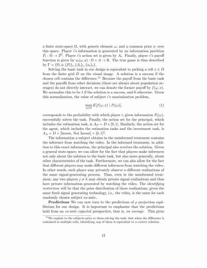
a finite state-space Ω, with generic element ω, and a common prior φ overthis space. Player i’s information is generated by an information partitionPi : Ω → 2Ω. Player i’s action set is given by Ai. Finally, player i’s payofffunction is given by ui(ω, a) : Ω×A→ R. The true game is thus describedby Γ = Ω, φ, Pii, Aii, uii.

Solving the basic task in our design is equivalent to picking a cell x ∈ Dfrom the finite grid D on the visual image. A solution is a success if thechosen cell contains the difference.11 Because the payoff from the basic taskand the payoffs from other decisions (these are always about population av-erages) do not directly interact, we can denote the former payoff by f(ω, x).We normalize this to be 1 if the solution is a success, and 0 otherwise. Giventhis normalization, the value of subject i’s maximization problem,

maxx∈D

E[f(ω, x) | Pi(ω)], (1)

corresponds to the probability with which player i, given information Pi(ω),successfully solves the task. Finally, the action set for the principal, whichincludes the estimation task, is AP = D× [0, 1]. Similarly, the action set forthe agent, which includes the estimation tasks and the investment task, isAA = D × [Invest, Not Invest]× [0, 1]2.

The information a subject obtains in the uninformed treatment containsthe inference from watching the video. In the informed treatment, in addi-tion to this exact information, the principal also receives the solution. Givena general state-space, we can allow for the fact that players make inferencesnot only about the solution to the basic task, but also more generally, aboutother characteristics of the task. Furthermore, we can also allow for the factthat different players may make different inferences from watching the video.In other words, each player may privately observe a different realizations ofthe same signal-generating process. Thus, even in the uninformed treat-ment, any two players j 6= k may obtain private signal realizations and thushave private information generated by watching the video. The identifyingrestriction will be that the prior distribution of these realizations, given thesame fixed signal generating technology, i.e., the video, is the same for eachrandomly chosen subject ex-ante..

Predictions We can now turn to the predictions of ρ projection equi-librium for our design. It is important to emphasize that the predictionshold from an ex-ante expected perspective, that is, on average. This gives

11We explain to the subjects prior to them solving the task, that when the difference iscontained in multiple cells, identifying any of them is equivalent to a correct solution.

12

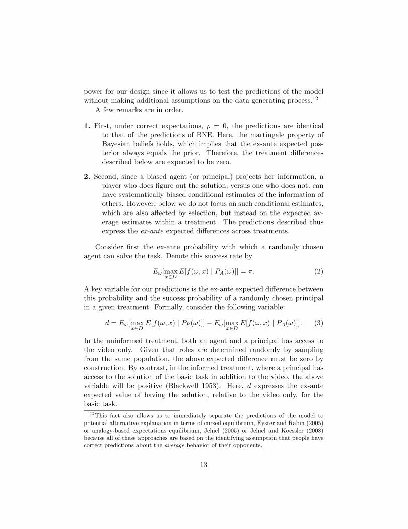
power for our design since it allows us to test the predictions of the modelwithout making additional assumptions on the data generating process.12

A few remarks are in order.

1. First, under correct expectations, ρ = 0, the predictions are identicalto that of the predictions of BNE. Here, the martingale property ofBayesian beliefs holds, which implies that the ex-ante expected pos-terior always equals the prior. Therefore, the treatment differencesdescribed below are expected to be zero.

2. Second, since a biased agent (or principal) projects her information, aplayer who does figure out the solution, versus one who does not, canhave systematically biased conditional estimates of the information ofothers. However, below we do not focus on such conditional estimates,which are also affected by selection, but instead on the expected av-erage estimates within a treatment. The predictions described thusexpress the ex-ante expected differences across treatments.

Consider first the ex-ante probability with which a randomly chosenagent can solve the task. Denote this success rate by

Eω[maxx∈D

E[f(ω, x) | PA(ω)]] = π. (2)

A key variable for our predictions is the ex-ante expected difference betweenthis probability and the success probability of a randomly chosen principalin a given treatment. Formally, consider the following variable:

d = Eω[maxx∈D

E[f(ω, x) | PP (ω)]]− Eω[maxx∈D

E[f(ω, x) | PA(ω)]]. (3)

In the uninformed treatment, both an agent and a principal has access tothe video only. Given that roles are determined randomly by samplingfrom the same population, the above expected difference must be zero byconstruction. By contrast, in the informed treatment, where a principal hasaccess to the solution of the basic task in addition to the video, the abovevariable will be positive (Blackwell 1953). Here, d expresses the ex-anteexpected value of having the solution, relative to the video only, for thebasic task.

12This fact also allows us to immediately separate the predictions of the model topotential alternative explanation in terms of cursed equilibrium, Eyster and Rabin (2005)or analogy-based expectations equilibrium, Jehiel (2005) or Jehiel and Koessler (2008)because all of these approaches are based on the identifying assumption that people havecorrect predictions about the average behavior of their opponents.

13

Below, we allow for role-specific degrees of projection, that is, the degreeof projection is ρ = (ρP , ρA) where ρP denotes the degree to the principalprojects and ρA the degree to which the agent project. At the end of thissection, we also restate the predictions of projection equilibrium for thecase where projection is homogenous, i.e., ρP = ρA, and thus the degree ofprojection is independent of the role a subject takes in the game.

Consider first a ρP -biased principal. The claim below describes the prin-cipal’s estimate of the agents’ success rate.

Claim 1 (Principal’s estimate). The principal’s expected estimate of thesuccess rate is given by π + ρPd.

Proof. See Appendix.

In the uninformed treatment, the principal’s estimate of the success rateis correct on average. A principal who solves the task and one who does notmight have systematically different and wrong conditional beliefs about theagent’s success probability. In the uninformed treatment, however, theseconditional mistakes cancel out on average. This is true because the ex-anteprobability with which a randomly chosen subject—independent of the roleassigned—figures out the solution is the same. In contrast, in the informedtreatment, the principal always has access to the solution. Because a biasedprincipal who knows the solution to the basic task acts as if she believed thatwith probability ρP the agent must know the solution for sure, the principalnow exaggerates the agent’s success rate on average. This exaggeration isincreasing both in the value of the principal’s additional information for thebasic task, d, and in the principal’s degree of projection, ρP .

We can now turn to the key prediction of the model and state the partialanticipation feature of projection equilibrium in our setup. Consider now aρA-biased agent. Given projection of degree ρP by the principal, the sec-ond claim implies a systematic difference between an agent’s estimate of theprincipal’s estimate and his own estimate of the average success rate in theinformed treatment, but not in the uninformed treatment, on average. Itpredicts that the difference between such second-order and first-order esti-mates should be greater in the informed treatment than in the uninformedtreatment.

Claim 2 (Agent’s estimate). The expected difference between the agent’sestimate of the success rate and the agent’s estimate of the principal’s meanestimate of the success rate is given by (1− ρA)ρPd.

Proof. See Appendix.

14

The above claim establishes that the agent anticipates the principal’sprojection but underestimates its extent on average. In more detail, theagent’s first-order estimate of π is unbiased in both treatments on average.In the uninformed treatment, the same holds for the second-order estimate,that is, the agent’s expected estimate of the principal’s mean estimate aswell. These facts are true for the same reason as in Claim 1: the agent andthe principal here are in a symmetric situation, each seeing only the video.By contrast, in the informed treatment, because d > 0, the agent’s estimateof the principal’s estimate is higher than his own on average. Let us describethis logic in more detail.

The agent assigns probability (1 − ρA) to the true distribution of theprincipal’s strategy. Hence in the informed treatment the agent antici-pates that the principal exaggerates the success rate by degree ρP on av-erage. At the same time, the agent is also biased and assigns probabilityρA to the principal—and also all other agents—being the projected versionand thus having the same information as he does. Since projection is all-encompassing, the projected version of the principal, who is real in a givenagent’s mind, is believed to know not only this given agent’s strategy, butalso share his beliefs about the strategies of all the other agents. Because anagent’s estimate of the strategies of the other agents is unbiased on average,the estimate attributed to the projected version of the principal will also beunbiased on average. In sum, the agent anticipates but underappreciates theextent to which an informed principal exaggerates the performance of thereference agents on average. Hence the agent underappreciates the informedprincipal’s exaggeration on average. The magnitude of this underapprecia-tion is increasing in the agent’s own bias. If the agent is fully biased, ρA = 1,then no exaggeration is anticipated on average. By contrast, if the agentis unbiased, ρA = 0, the agent has correct beliefs about the principal’s ex-pected estimate on average. The agent’s average underappreciation is thusincreasing in ρA.

Finally, as long as the agent is not fully biased, the above claim on antic-ipation implies the following comparison of the agent’s propensity to choosethe investment option over the sure payoff between the two treatments.

Claim 3 (Agent’s investment choice). The agent’s propensity to invest islower when matched with an informed as opposed to an uninformed principalon average.

This claim holds qualitatively as long as the principal is biased and theagent is not fully biased. The result follows from the fact that the value of theinvestment in the uninformed treatment first-order stochastically dominates

15

the value of the investment in the informed treatment. Because of the agent’santicipation, it then follows that the agent has a greater incentive to investin the relationship in the uninformed treatment than in the informed one.

Homogenous Projection We can now return to the case of homoge-nous projection, where the agent and the principal are equally biased. Letagain ρA = ρP = ρ. Here the principal’s exaggeration in Claim 1 is gov-erned by ρ, the perceived probability that an agent is a projected version.The agent’s anticipation is governed by (1− ρ)ρ – the agent’s perception ofthe probability that the principal assigning to the agent being the projectedversion. When estimating the model we will do so both under homogenousprojection and under role-specific heterogeneous projection.

4 Results

We embark on the analysis by testing whether the principals’ expectations ofthe agents’ performance is affected by the information conditions (Claim 1).We then investigate whether the agents’ investment choices (Claim 3) aswell as their second-order beliefs (Claim 2) reflect anticipation of differentperformance expectations by differentially informed principals. Finally, weexplore to which extent the data can be accommodated by projection equi-librium (Madarasz 2014a).

4.1 Principals

Figure 3 shows the distribution of individual performance estimates by in-formed and uninformed principals together with the actual performance ofthe reference agents. The figure clearly supports Claim 1. First, unin-formed principals are, on average, very well calibrated: there is virtually nodifference between their average estimate (39.76%) and the average perfor-mance of the reference agents (39.25%; p = 0.824).13 In contrast, informedprincipals overestimate the performance of the reference agents for the vastmajority of tasks.14 Their average estimate of the success rate amounts to57.45% which is significantly higher than both the actual performance of the

13We employed a t-test of the average estimate per principal against the average successrate (over all tasks). A Kolmogorov-Smirnov test of the distributions of average individualestimates between treatments yields p = 0.001. Unless stated otherwise, p-values through-out the result section refer to (two-sided) t-tests that are based on average statistics persubject.

14Figure 7 in the Appendix provides a plot of the principals’ average first-order beliefper treatment over time.

16

0.0

0.1

0.2

0.3

0.4

0.5

0.6

0.7

0.8

0.9

1.0

Cum

ula

tive

dis

trib

uti

on funct

ion

0.0 0.1 0.2 0.3 0.4 0.5 0.6 0.7 0.8 0.9 1.0

Average first-order belief (estimate of the success rate) per principal

Uninformed principal

Informed principal

Tru

e su

cces

s ra

te

Figure 3: Distribution of average first-order beliefs per principal in the in-formed and the uninformed treatment.

reference agents (p < 0.001) and the average estimate of uninformed prin-cipals (p < 0.001).15 Informed principals overestimating the agents’ perfor-mance by more than 18 percentage points led to significantly lower expectedearnings of informed principals (e 2.40) than uninformed principals (e 3.65;one-sided t-test: p = 0.034).16 We record our findings in support of Claim1 in

Result 1. Informed principals state significantly higher expectations regard-ing the performance of the reference agents than uninformed principals. In-

15Principals in the uninformed treatment who spotted the difference in the task alsooverestimated the success of the reference agents (60.93%). Principals who have thesolution think the task was easier for the agents than it actually was, regardless of whetherthe solution was given right away as in the informed treatment or found by the principalsthemselves. The projection equilibrium framework predicts this finding. The magnitudeof the uninformed principals’ overestimation cannot be directly compared to that of theinformed principals, because of the self-selection issue. The uninformed principals whosolved the task could be more skilled on average. Thus, we focus on the comparisonsbetween the treatments rather than within treatments.

16The average payoffs in the rounds randomly selected for payment were e 1.50 ande 2.50 in the informed and the uninformed treatment, respectively.

17

formed principals, but not uninformed principals, overestimate the perfor-mance of the reference agents on average.

Following Moore and Healy (2008), we can also examine the extent towhich task difficulty per se plays a role in our analysis. If we divide our tasksinto hard and easy tasks by using the median task difficulty as the cutoff(yielding 10 hard tasks with success rates of 0.42 and below and 10 easy taskswith success rates of 0.43 and above), we find that uninformed principals,on average, overestimate the actual success rate for hard tasks (p=0.047,sign test) but also underestimate the true success rate for easy tasks (p =0.059). This reversal is well known as the hard-easy effect first establishedby Moore and Healy (2008). This reversal, however, is not observed forinformed principals who significantly overestimate the true success rate forany task, irrespective of the degree of difficulty (p=0.012 and p=0.0069 forhard and easy tasks, respectively).

The systematically biased forecasts in Result 1 are not surprising givenprevious findings in the literature (Loewenstein et al., 2006) and it also con-firms the basic premise of our design.17 We can now turn to the new aspectof our design which is the carful testing of the simultaneous anticipation ofthis phenomenon.

4.2 Agents

4.2.1 Investment decisions

We move on to the agents’ investment choices. Remember, for the agentsthe only difference between the two treatments is that agents matched toinformed principals were told that their principal had access to the solutionwhile agents in the uninformed treatment were told that their principal hadnot seen the solution when forming his performance expectation. Figure 4shows the distribution of individual investment rates in the informed andthe uninformed treatment.

The figure reveals a clear pattern. Agents matched to informed princi-pals invest at a considerably lower rate than agents matched to uninformed

17If the solution to the task altered the informed principals’ ex-ante perception of thetask in other ways, the average estimate of the agents’ performance across the two treat-ments should still be equal under the Bayesian framework even if the distributions are notexactly the same.

18

0.0

0.1

0.2

0.3

0.4

0.5

0.6

0.7

0.8

0.9

1.0

Cum

ula

tive

dis

trib

uti

on funct

ion

0.0 0.1 0.2 0.3 0.4 0.5 0.6 0.7 0.8 0.9 1.0

Individual investment rate

Agents matched touninformed principals

Agents matched toinformed principals

Figure 4: Distribution of individual investment rates in the informed andthe uninformed treatment.

principals.18,19 The treatment difference is not only statistically significant;the magnitude of the difference is also economically relevant. The aver-age investment rate of agents matched to uninformed principals is 67.3%,whereas the average investment rate of agents matched to informed prin-cipals is only 39.2% (p < 0.001). The investment rate in each treatmentis remarkably close to the fraction of cases where the investment pays offin each treatment, i.e., where the principals’ expectations do not exceedthe agents’ success rate by more than 10 percentage points. Specifically, ifagents knew the estimate of their principal (and best responded to this in-

18We find no significant treatment difference in the performance of agents (their successrate is 41.35% in the informed treatment and 39.89% in the uninformed treatment; p =0.573). Thus, any treatment differences in the agents’ investment decision or the agents’beliefs cannot be attributed to differences in task performance.

19We pool the sessions with belief elicitation and those without. Within the informed[uninformed] treatments, the average investment rates per agent in sessions with beliefelicitation do not differ from the average investment rates in sessions without belief elic-itation (t-test, p = 0.76 [p = 0.70]). There are also no significant time trends in theinvestment rates (see Figure 8 in the Appendix).

19

Table 2: Regressions of individual investment rates on treatment, gender, and riskattitude.

Dependent variable Individual investment rate

(OLS) (1) (2) (3) (4) (5)

Treatment −0.281∗∗∗ −0.279∗∗∗ −0.255∗∗ −0.259∗∗∗ −0.254∗∗

(1-informed) (0.075) (0.075) (0.102) (0.077) (0.102)

Gender −0.059 −0.032 −0.048(1-female) (0.075) (0.108) (0.109)

Treatment×Gender −0.053 −0.009(0.151) (0.157)

Coef. risk aversion −0.026 −0.024(DOSE) (0.022) (0.023)

Constant 0.673∗∗∗ 0.698∗∗∗ 0.687∗∗∗ 0.695∗∗∗ 0.715∗∗∗

(0.053) (0.063) (0.071) (0.057) (0.076)

N 94 94 94 94 94R2 0.134 0.140 0.141 0.147 0.151F 14.230 7.390 4.920 7.813 3.960

Note: Values in parentheses represent standard errors. Asterisks represent p-values: ∗p < 0.1,∗∗p < 0.05, ∗∗∗p < 0.01.

formation), they would, on average, invest in 66.9% of the cases when beingmatched to an uninformed principal but only in 38.1% when being matchedto an informed principal.

Table 2 reports the results of regressions of the investment rate per sub-ject on a constant, a treatment dummy, a gender dummy, and individual riskattitudes. The estimation results corroborate the previous finding. First,the treatment effect remains significant and similar in size when we controlfor gender and individual risk attitude. Second, subjects with higher degreesof risk aversion tend to invest less often (columns 4 and 5) but this effectis not significant. Finally, the treatment effect is significant for both maleand female subjects, with female subjects investing slightly (but not signifi-

20

cantly) less often than male subjects (columns 2, 3, and 5).20 We summarizeour findings in

Result 2. Agents invest significantly less often when they are matched toinformed principals than when they are matched to uninformed principals.

Result 2 is consistent with agents anticipating the projection of informedprincipals. The agents shy away from investing, that is, from choosing anoption whose payoff depends negatively on the level of the principal’s per-formance expectations.

At this point other explanations for the treatment difference in invest-ment choices might come to mind that do not posit that the agents antici-pate the projection of informed principals. Specifically, models of stochasticchoice with differential assumptions about the rate at which subjects makeerrors in their choices—while assuming that agents in both treatments en-tertain the same beliefs about the principals’ estimates on average—mightexplain the lower investment rate of agents in the informed treatment.21 Aswe will see in the following section, such alternative explanations are clearlyruled out by the analysis of the agents’ stated beliefs.

4.2.2 Stated beliefs

Collecting information about higher-order beliefs is essential to test equilib-rium theories. We elicited agents’ first-order beliefs, i.e., their own estimatesof the success rate, and their second-order beliefs, i.e., their estimate of theirprincipal’s estimate of the success rate. According to Claim 2, the agents’first-order beliefs are expected to be correct on average in both treatments,and the agents’ second-order beliefs are expected to reflect partial anticipa-tion of the informed principals’ biased performance expectations. Figure 5shows a bar chart of the average stated beliefs of the agents in each treat-ment together with the average performance of the reference agents and thecorresponding estimates of the principals.

The figure summarizes our key findings. The left-hand bars on eachpanel (first-order beliefs) show that the agents are well calibrated in both

20There is no significant interaction between the treatment and having completed a tasksuccessfully. The treatment effect on investment decisions is significant both for periodsin which the agents solved the task and for periods in which the agents did not solve thetask. For further details see Table 4 in the Appendix.

21In principle, this idea can be captured by quantal response equilibrium (QRE) withdifferent precision parameters between treatments—either on the side of the agents orthe principals. Note, however, that QRE is not suited to explain the biased estimates ofinformed principals in the first place (or any anticipation thereof).

21

0.0

0.1

0.2

0.3

0.4

0.5

0.6Succ

ess

rate

Uninformed treatment Informed treatment

Ag

ents

: Sec

on

d-o

rder

bel

iefs

Pri

nci

pal

s: F

irst

-ord

er b

elie

fs

Ag

ents

: Fir

st-o

rder

bel

iefs

Ag

ents

: Fir

st-o

rder

bel

iefs

Ag

ents

: Sec

on

d-o

rder

bel

iefs

Pri

nci

pal

s: F

irst

-ord

er b

elie

fs

True success rate

Figure 5: Agents’ first-order beliefs (estimates of the success rate) andsecond-order beliefs (estimates of the principals’ estimate), conditional onbeing matched with informed or uninformed principals. Capped spikes rep-resent 95% confidence intervals.

treatments: their estimates of the success rate are correct on average and notsignificantly different between treatments (p = 0.956).22 The middle barsreveals that the agents’ second-order beliefs are somewhat higher than theirfirst-order beliefs in either treatment.23 That is, in both information condi-tions the agents tend to expect that the principals are somewhat more op-timistic regarding the reference agents’ performance than themselves. How-ever, as predicted by Claim 2, this effect is significantly stronger in the in-formed treatment than in the uninformed treatment: First, the second-orderbeliefs of agents matched to informed principals (51.14%) are significantly

22The average success rate in the first ten tasks (where we elicited the agents’ beliefs)is 40.0%. The agents’ average estimate of the success rates in the first ten tasks is 39.72%(p = 0.917) in the uninformed treatment and 39.91% (p = 0.967) in the uninformedtreatment.

23In the uninformed treatment, none of the elicited beliefs are, on average, significantlydifferent from the true success rate: neither the agents’ first-order beliefs (p = 0.917),their second-order beliefs (p = 0.140), nor the principals’ estimates (p = 0.337).

22

higher than those of agents matched to uninformed principals (44.15%; one-sided t-test: p = 0.031). Second, the individual differences between second-and first-order beliefs are significantly larger for agents matched to informedprincipals than for agents matched to uninformed principals (p < 0.001).24,25

A further key finding can be taken from Figure 5. Although the second-order beliefs of agents in the informed treatment are significantly higherthan the actual success rate, they are, on average, also significantly lowerthan the informed principals’ estimates (one-sided t-test: p = 0.047). Thatis, the agents appear to anticipate the projection of the informed principals,but not to its full extent. This finding is consistent with the predictions ofprojection equilibrium.

Result 3 (Partial anticipation of information projection). The agent’s es-timate of the success rate (first-order belief) is correct on average in bothtreatments. The average difference between the agent’s estimate of the prin-cipal’s estimate (second-order belief) and her own estimate (first-order be-lief) is significantly larger the in the informed treatment than in the unin-formed treatment. In the informed treatment, the agent’s estimate of theprincipal’s estimate of the success rate (second-order belief) is, on average,between her own estimate and the principal’s estimate.

We have presented evidence that is qualitatively consistent with the pre-dictions of Section 3. In particular, informed principals, but not uninformedones, exaggerated the success rate of agents (Claim 1). Agents matchedwith informed principals, but not with uninformed ones, partially antici-pated that their principals overestimated the reference agents’ success rateson the tasks (Claim 2). Furthermore, agents were less likely to invest whenmatched with an informed principal than when matched with an uninformedprincipal (Claim 3). In the next section we conduct a quantitative test ofthe descriptive power of projection equilibrium.

24This treatment difference is robust when controlling for individual characteristics (seeTable 5 in the Appendix) and significant both for instances where the agents solved thetask and where they did not solve the task (see Table 6 in the Appendix).

25We find no significant interaction between the treatment and having completed a tasksuccessfully. The treatment effect on the individual differences between first- and second-order estimates is significant both for periods in which the agents solved the task and forperiods in which the agents did not solve the task. For further details, see Table 6 in theAppendix.

23

4.3 Estimation of projection equilibrium parameters

How well can the data be accommodated by a single-parameter extensionof Bayesian Nash Equilibrium? In the most parsimonious parametrizationof projection equilibrium, both the principal’s exaggeration and the agent’sunderestimation of the principal’s projection are governed by the same pa-rameter ρ. In the following we identify the levels of projection on both sidesthat would be consistent with the beliefs we elicited. We then test whetherthe estimated projection is significantly different across player roles.

Claims 1 and 2 provide the equations to estimate the projection param-eter of the principals and the agents in the informed treatment. We startwith a flexible specification that allows for different degrees of projectionbias between roles as well as within roles, where we denote the average de-gree of projection in the principal population by ρPµ and that in the agent

population by ρAµ . Following Claim 1, an informed principal i—who solves

the task with probability 126—has the following expected belief bP1,i,t of thesuccess rate πt in task t

E(bP1,i,t | πt, ρPi ) = πt + ρPi (1− πt) =: µPit . (4)

Following Claim 2, agent j’s expected second-order belief bA2,j,t about herinformed principal’s mean estimate, conditional on her (unbiased) first-orderbelief, is given by

E(bA2,j,t | bA1,j,t = πt, ρAj ) = bA1,j,t + (1− ρAj )ρPµ (1− bA1,j,t) =: µAj,t. (5)

To account for the fact that subjects’ stated beliefs fall in a boundedinterval between zero and one, we employ a beta regression model. Specif-ically, we assume that subjects’ responses bP1,i,t and bA2,j,t follow a beta dis-tribution with task- and individual-specific mean (4) and (5), respectively.With slight abuse of notation we write bkit for subject i’s stated belief inrole k, where bkit = bP1,i,t for principals (k = P ) and bkit = bA2,i,t for agents

(k = A). With beta-distributed responses bkit, the probability of observingbelief bkit of subject i in role k can be written as:27

f(bkit;µkit, φb) =

Γ(φb)

Γ(φbµkit)Γ(φb(1− µkit)))

(bkit)φbµ

kit−1(1− bkit)φb(1−µ

kit)−1,

26Following the derivation of Claim 1 and Claim 2, we calculate dt—the differencebetween the ex-ante probability of solving task t for an informed principal and for anagent—by subtracting the empirical success rate of the reference agents for each taskfrom 1—approximately the success rate of informed principals.

27See Ferrari and Cribari-Neto (2004). A link function as in standard beta regressionmodels is not needed because (4) and (5) map (0, 1) −→ (0, 1) for ρ ∈ [0, 1) and πt, b

A1,i,t ∈

(0, 1). Abstaining from using a link function has the advantage that we can interpret

24

where φb is a precision parameter that is negatively related to the noise insubjects’ response.

To capture unobserved individual heterogeneity in the projection pa-rameters and to account for repeated observations on the individual level,we employ a random coefficients model. Specifically, we assume that theindividual-specific degree of projection ρki ∈ [0, 1], k ∈ A,P follows a betadistribution with role-specific mean ρkµ and density

g(ρki ; ρkµ, φρ) =

Γ(φρ)

Γ(φρρkµ)Γ(φρ(1− ρkµ)))

(ρki )φρρ

kµ−1(1− ρki )φρ(1−ρkµ)−1,

where the parameter φρ is negatively related to the variance of projectionbias in the principal and the agent population.

We now formulate the log-likelihood function. Conditional on ρki and φρ,

the likelihood of observing the sequence of stated beliefs (bkit)t of subject iin role k is given by

Lki (ρki , φb) =

∏t f(bkit;µ

kit(ρ

ki ), φb).

Hence, the unconditional probability amounts to

Lki (ρkµ, φρ, φb) =

∫ [∏t f(bkit;µ

kit(ρ

ki ), φb)

]g(ρki ; ρ

kµ, φρ)dρ

ki . (6)

The joint log likelihood function of the principals’ and the agents’ responsescan then be written as

lnL(ρPµ , ρAµ , φρ, φb) =

∑k

∑i logLki (ρ

kµ, φρ, φb). (7)

We estimate the the parameters in (7) simultaneously by maximum sim-ulated likelihood (Train 2009; Wooldridge, 2010).28

Table 3 shows the estimation results for the unrestricted model as well asfor the restricted model with ρµ = ρPµ = ρAµ . We make three observations.29

the estimated parameters ρPµ and ρAµ directly as parameters of projection from Claims 1

and 2. As in standard beta regression models, observations of ykit = 0 or ykit = 1 have alikelihood of 0 and can therefore not be used in maximum likelihood estimation. However,the entire data set has only one observation of ykit = 1 (one of the principals’ first-orderbeliefs is bP1,i,t = 1). We drop this observation in the estimation. Treating this observation

as bP1,i,t = bP1,i,t − ε, ε = 10ˆ(−10) yields similar results.28The estimation is conducted with GAUSS. We use Halton sequences of length R =

100, 000 for each individual with different primes as the basis for the sequences for theprincipals and the agents.

29The results are robust with respect to alternative starting values for the estimationprocedure. All regressions for a uniform grid of starting values converge to the same esti-mates (both for the restricted and the unrestricted model). Thus, the likelihood functionin (7) appears to assume a global (and unique) maximum at the estimated parameters.

25

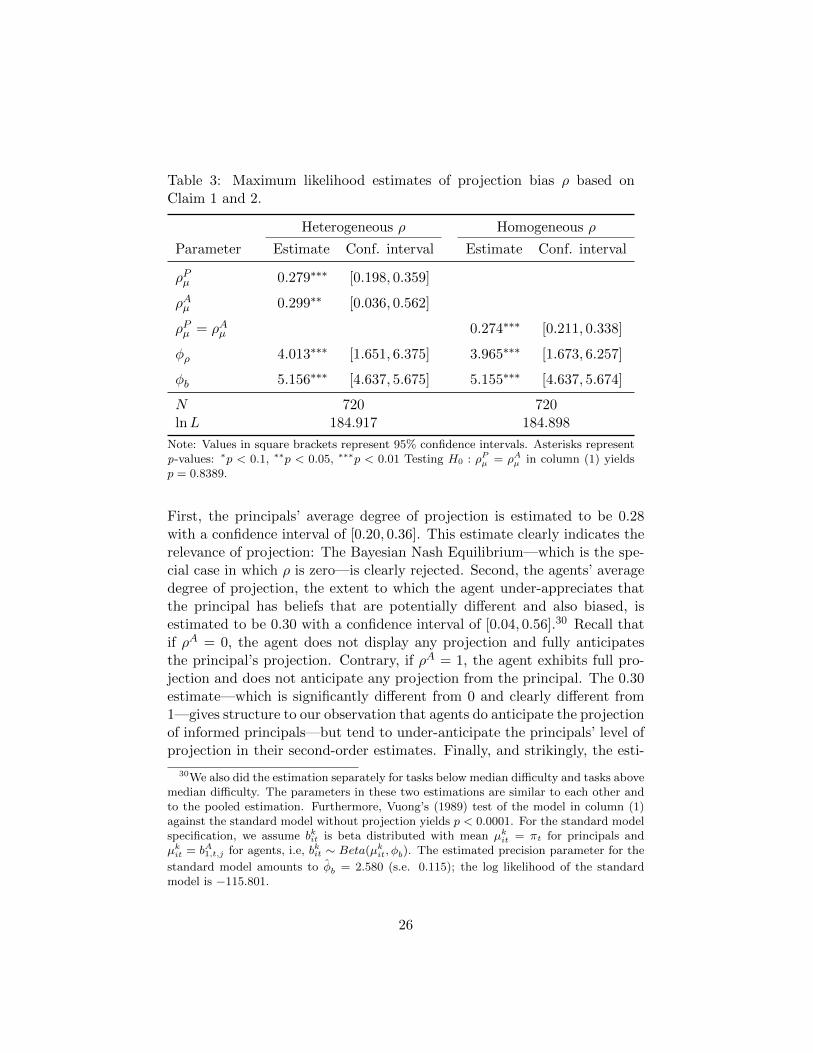
Table 3: Maximum likelihood estimates of projection bias ρ based onClaim 1 and 2.

Heterogeneous ρ Homogeneous ρ

Parameter Estimate Conf. interval Estimate Conf. interval

ρPµ 0.279∗∗∗ [0.198, 0.359]

ρAµ 0.299∗∗ [0.036, 0.562]

ρPµ = ρAµ 0.274∗∗∗ [0.211, 0.338]

φρ 4.013∗∗∗ [1.651, 6.375] 3.965∗∗∗ [1.673, 6.257]

φb 5.156∗∗∗ [4.637, 5.675] 5.155∗∗∗ [4.637, 5.674]

N 720 720lnL 184.917 184.898

Note: Values in square brackets represent 95% confidence intervals. Asterisks representp-values: ∗p < 0.1, ∗∗p < 0.05, ∗∗∗p < 0.01 Testing H0 : ρPµ = ρAµ in column (1) yieldsp = 0.8389.

First, the principals’ average degree of projection is estimated to be 0.28with a confidence interval of [0.20, 0.36]. This estimate clearly indicates therelevance of projection: The Bayesian Nash Equilibrium—which is the spe-cial case in which ρ is zero—is clearly rejected. Second, the agents’ averagedegree of projection, the extent to which the agent under-appreciates thatthe principal has beliefs that are potentially different and also biased, isestimated to be 0.30 with a confidence interval of [0.04, 0.56].30 Recall thatif ρA = 0, the agent does not display any projection and fully anticipatesthe principal’s projection. Contrary, if ρA = 1, the agent exhibits full pro-jection and does not anticipate any projection from the principal. The 0.30estimate—which is significantly different from 0 and clearly different from1—gives structure to our observation that agents do anticipate the projectionof informed principals—but tend to under-anticipate the principals’ level ofprojection in their second-order estimates. Finally, and strikingly, the esti-

30We also did the estimation separately for tasks below median difficulty and tasks abovemedian difficulty. The parameters in these two estimations are similar to each other andto the pooled estimation. Furthermore, Vuong’s (1989) test of the model in column (1)against the standard model without projection yields p < 0.0001. For the standard modelspecification, we assume bkit is beta distributed with mean µkit = πt for principals andµkit = bA1,t,j for agents, i.e, bkit ∼ Beta(µkit, φb). The estimated precision parameter for the

standard model amounts to φb = 2.580 (s.e. 0.115); the log likelihood of the standardmodel is −115.801.

26

mated parameters of projection are not significantly different between theprincipals and the agents (p = 0.839). Given the similarity between the es-timated parameters in the unrestricted model, the log likelihood of the twomodels are very close, and standard model selection criteria clearly favorthe single-parameter model of homogeneous projection over the model withtwo parameters (BIC).

4.4 Individual heterogeneity

The final part of the analysis is devoted to test of the predictions of pro-jection equilibrium on the individual level in conjunction with a test of theeconometric specification of model (7). Specifically, we test whether themean projection bias ρµ = 0.274 estimated from (7) is indeed generated bya beta distribution of ρi or, alternatively, whether individual heterogeneityin projection bias is better described by some other distribution. A mis-specification in this matter would not only be relevant from an econometricpoint of view; it might also challenge the economic interpretation of our re-sults. If, for example, the estimate of the mean projection bias was a resultof a finite mixture of some agents not anticipating information projection atall (ρ = 1) and the remaining agents fully anticipating information projec-tion (ρ = 0), then model (7) would be misspecified and, more importantly,Claim 2 (partial anticipation of information projection) would have littleempirical bite on the individual level.

We base our specification test on non-parametric density estimates ofindividual projection bias in the principal and the agent population. To thisend, we first obtain individual estimates of the projection bias parameter ρfor each principal and agent in the informed treatment, where we employthe most simple and straightforward estimation technique without imposingany restrictions on the parameter ρ. Specifically, for each informed principali, we estimate his projection bias ρPi from

bP1,i,t = πt + ρPi (1− πt) + εit, (8)

where bP1,i,t denotes the principal’s expectation of the success rate πt in taskt, and εit denotes an independent and normally distributed error term withmean zero and variance σ2

i . Analogously, for each agent j in the informedtreatment we estimate her projection bias ρAj from

bA2,j,t = bA1,j,t + (1− ρAj )ρPµ (1− bA1,j,t) + εjt, (9)

where bA1,j,t denotes the agent’s estimate of the success rate in task t (first-

order belief), bA2,j,t denotes her estimate of the principal’s estimate (second-

27

order belief), ρPµ denotes the mean projection bias in the principal popula-tion, and εjt denotes an independent and normally distributed error withmean zero and variance σ2

j . We estimate the parameters in (8) and (9) by

linear least squares, where we substitute ρPµ in (9) with the average estimate

of ρPi obtained from the regressions in (8).31

0.0

0.1

0.2

0.3

0.4

0.5

0.6

0.7

0.8

0.9

1.0

Cum

ula

tive

dis

trib

ution funct

ion

-0.6 -0.4 -0.2 0.0 0.2 0.4 0.6 0.8 1.0 1.2

Estimated projection bias ρ

Principals

Agents

Figure 6: Cumulative distribution functions (CDF) of principals’ (solid) andagents’ (dashed) projection bias ρ in the informed treatment. Black linesrepresent empirical CDFs; gray lines represent best-fitting beta CDFs.

Figure 6 shows the empirical cumulative distribution functions (CDFs)of individual projection bias in the principal and the agent population. A ca-sual inspection of the figure shows that the empirical CDFs of the principals’and the agents’ ρ are quite similar. In fact, a Kolmogorov-Smirnov test doesnot reveal any significant difference between the distributions (p = 0.441).That is, not only the average projection bias by the principals and the agents

31Because we use an estimate of ρPµ in the estimation of the agents’ projection bias, thecomposite error term in equation (9) is heteroscedastic. We therefore base all inferenceon the individual level on heteroscedasticity-robust standard errors. Unlike in the simul-taneous estimation of the agents’ and the principals’ projection bias from (7), the simpleestimation approach applied here assures that the individual estimates of the principals’projection bias are not informed by the data of the agents’ choices, a feature that is verydesirable for our specification test below.

28

is the same; also the distributions of the principals’ and the agents’ projec-tion bias are the same. These findings lend strong support for a key featureof projection equilibrium—that information projection and the anticipationthereof are governed by the same parameter.

Figure 6 conveys a second important message regarding the econometricspecification in (7). The empirical CDFs of principals’ and the agents’ pro-jection bias are very well described by beta distributions (the gray lines in thefigure show the best-fitting beta distributions).32 Moreover, the joint empir-ical CDF of the principals’ and the agents’ projection bias is not significantlydifferent from the beta distribution g(ρµ = 0.274, φρ = 3.965) obtained frommodel (7) with homogeneous projection (see Table 3; Kolmogorov-Smirnovtest: p = 0.063). That is, our non-parametric estimate of the distributionof individual projection bias clearly supports the beta specification withrespect to individual heterogeneity in (7).

A final crucial observation that can be taken from Figure 6 is that—inline with Claim 2—most agents appear to anticipate the information pro-jection by the principals—but not too its full extent (ρAj ∈ (0, 1) for mostagents). This observation is backed up by tests of the estimated projectionparameters against zero and one. For both the principals and the agents, themost frequently observed category is the one where ρ is estimated to be sig-nificantly larger than zero but also significantly smaller than 1.33 That is, themost prevalent behavioral pattern is significant—but not full—informationprojection and at the same time significant—but not full—anticipation ofinformation projection.34

32Kolmogorov-Smirnov tests of the empirical CDF against the best-fitting beta distri-bution (as shown in Figure 6) yields p = 0.941 for the principals and p = 0.584 for theagents.

3370.8% of the principals and 50% of the agents fall in this category. The second mostcommon category in both populations is the one of ρ being not significantly different from0 but significantly different from 1, i.e., no information projection and at the same timefull anticipation of others’ information projection (25% of the principals and 37.5% ofthe agents). Finally, a few agents (12.5%) exhibit an estimated ρ that is not significantlydifferent from 1 but significantly different from 0, i.e., they do not anticipate the principals’information projection at all. Although the estimated mass on the same category in theprincipal population (full projection) is zero, the difference is based on three observationsonly. In fact, in line with the previous findings there is no significant difference betweenthe agents’ and the principals’ categorized distribution of projection bias (Fisher’s exacttest: p = 0.124).

34We also performed a model-free estimation of each agent’s degree of anticipation αjby estimating the weight in bA2,j,t = (1 − αj)bA1,j,t + αjb

P1,t + εjt, where bP2,t =

∑j bP1,i,t is

the principals’ average estimate of the success rate in task t. The categorized estimateddistribution of αj is qualitatively similar to the corresponding distribution of (1 − ρAj ).

29

5 Conclusion

A host of robust findings demonstrate that people engage in limited infor-mational perspective-taking. This study is the first to document people’santicipation of such mistakes in the thinking of others. We find not onlythat better-informed principals project their information onto agents, butalso that lesser-informed agents anticipate the principals’ bias as evincedby their decision to insure against the principals’ overestimation of success.The second-order estimates show that an agent in our experiment under-stands that the principal has a belief about the agent’s perspective which issystematically different from the agent’s true perspective.

The findings support the logic of projection equilibrium which integratesthis basic phenomenon with such higher-order perceptions. While informa-tional projection biases one’s belief about the perspectives of others, ouranticipation result shows that a person is at least partially sophisticatedabout the fact that differentially informed others have biased beliefs abouther perspective on average. Such sophistication is partial due to a person’sown projection: agents underappreciate the degree to which principals ex-aggerate their success rate due to the agents’ own mistake. In support ofthe logic of this solution concept, we find that the extent to which informedprincipals overestimate the agents’ success rate is very similar in magni-tude to the extent to which lesser-informed agents under-appreciate suchover-estimation.

5.1 Relation to Alternative Models and Mechanisms

Unlike a number of other behavioral game theory models of private infor-mation games, projection equilibrium focuses on the players misperceivingother players’ information per se, rather than misperceiving the relation-ship between other players’ information and their actions. In particular,the models of Jehiel and Koessler (2008) and Eyster and Rabin (2005) as-sume that people have coarse or misspecified expectations about the link

First, the majority of agents (54.2%) exhibit an estimated αj that is significantly largerthan zero but also significantly smaller than 1. That is, their estimate bA2,j,t of the princi-pal’s estimate of the success rate is, on average, between their own estimate bA1,j,t and theaverage estimate of the principals bP1,t. In other words, most agents partially anticipatethe projection of informed principals. Further 25.0% of the agents fall into the categoryof αj = 0 with no anticipation of information projection (bA2,j,t = bA1,j,t), and 16.7% ofthe agents fall into the category of αj = 1 exhibiting full anticipation (bA2,j,t = bP1,t). Theremaining 4.2% correspond to an agent whose estimated αj is not significantly differentfrom both zero and one.

30

between others’ actions and their information, but these models are closedby the assumption that those expectations are correct on average. In turn,in the context of the current experiment, these models imply that a principalshould never exaggerate the agent’s performance on average and the agentshould never anticipate any mistake by the principal on average. Hence,just as the BNE, they predict a null affect for both hypothesis tested in thispaper.35

Although we find no evidence that risk aversion matters for the subjectschoices, note also that since more information helps unbiased principal’smake more accurate forecasts on average, under correct beliefs and riskaversion the agent should be choosing the lottery over the safe option moreoften when the principal is informed rather than when she is not. Insteadwe find the opposite.

Finally, note that overconfidence cannot explain the subjects choices ei-ther. If an agent believes that she is better than average, then she will simplyexaggerate the return from choosing the investment option as opposed to thesure payment, but this will not differ across treatments. Similarly a principalmay be over- and under-confident when inferring about other’s performanceon a given task, but there is no reason for this to systematically interactwith the treatment per se.

5.2 Future Directions

Our simple experimental setup can be used to study a number of interestingquestions related to the phenomenon of information projection. For exam-ple, to what extent might principals anticipate their biased estimation of theagents’ performance and opt out of receiving the solutions when given thechoice? Additionally, in our study, the principals do not receive any feed-back about the agents’ choices and the agents do not receive any feedbackabout the principals’ estimations. Future experimental work could studyhow different levels of feedback might affect how the principals adjust theirestimations and how the agents change the extent of their anticipation.

Naivete about one’s own tendency combined with partial sophisticationabout others’ tendency to project information has potentially importanteconomic implications in agency and strategic settings more generally. Con-sistent with the discussion in Berlin (2003), our results imply that people notsimply exaggerate the extent to which others have the same information as

35Note also that QRE predicts the null of no treatment difference since the principal’sincentives in the two treatments are exactly the same.

31

they do, but anticipate that others’ belief about their perspective systemat-ically differs from the perspective they truly have. Our investment decisioncan be interpreted as the agents’ valuation of the relationship with the prin-cipal. The greater is the information gap between the principal’s informationwhen monitoring and the agent’s true information, the less the agent willvalue the relationship. If agents have to sort into various jobs in the labormarket, such anticipation will affect the decision and may induce people towork without principals when principals monitor with ex-post information;here monitoring increases rather than decreases agency costs. Our resultsmay help explain a firm’s desire to limit the use of subjective performancemeasures based on ex-post information in combination with objective per-formance measures that would otherwise be optimal in a Bayesian setting(Baker et al.,1994) and provides a cognitive reason why such evaluationsmight often be biased. This affects the Bayesian results on the optimal useof information and incentives (Holmstrom, 1979). In our setting, greaterscrutiny directly biases learning leading to wrong judgments and system-atically lower payoffs. Importantly, the type of reasons identified in theliterature under rational expectations whereby more information backfiresin agency settings with dynamic career concerns (e.g., Scharfstein and Stein,1990; Cremer, 1995; Prat, 2005) will typically require different contractualsolutions than those used for the anticipation of projection.

Our design could be extended to study other information and incen-tive schemes and further contribute empirically to the growing literatureon incorporating behavioral assumptions into the understanding of decision-making in firms (e.g., Camerer and Malmendier 2007; Malmendier and Tate,2008; Spiegler, 2011). In context of negligence liability or patent law, whereprojection will systematically distort judgements made in hindsight (Harley,2007), anticipating it may further distort the ex-ante incentives for effort orinvestment into innovation. Importantly, the fact that anticipation is partialmeans that the extent to which an ex-ante designer would want to correct forthe presence of this mistake, for example in the design of legal institutions,might be insufficient.

The paper also lends support to the notion of projection equilibrium forthe analysis of games with informational differences. Future research caninvestigate its predictions for a great variety of settings both theoreticallyand empirically. Here key implications may depend on the extent to whichpeople anticipate the projection of others. For example, Madarasz (2014b)applies the idea of informational projection to dynamic bargaining and showsthat the anticipation of even a small amount of this mistake can have a sig-nificant impact on bargaining outcomes and the optimal selling mechanism

32

(Myerson, 1981). It would be interesting to know the extent to which thismistake and its anticipation may play a significant role in communicationor coordination problems.

Finally, our results speak to the importance of understanding the con-sequences of established forms of biased beliefs (DellaVigna, 2009; Mobiuset al., 2014) being anticipated by others. Indeed, while there are multiplefactors that might generate biased beliefs, it is the patterns in higher-orderbeliefs, beliefs about those biases, that give us more insight into the leadingfactors. For example, if informed players exaggerated the performance ofuninformed players because everyone thinks others are just like them, thenit is harder to account for the partial anticipation of this exaggeration bythe agents as predicted by projection equilibrium and established by ourfindings. In other contexts with biased beliefs about one’s own choices, suchas naivete about self-control problems (O’Donoghue and Rabin, 1999), or aperson’s failure to appreciate the full extent to which she will be subject tothe endowment effect (Kahneman et al.,1990; Loewenstein and Adler, 1995)as her reference point shifts, people might be better at anticipating the mis-takes of others (Van Boven et al., 2003). This would then affect implicationsfor trade, delegation, and optimal contracting more generally.

33

References

[1] Akerlof, G. A. (1970): “The Market for “Lemons”: Quality Uncertaintyand the Market Mechanism,” Quarterly Journal of Economics, 84(3),488–500.

[2] Alchian, A. A., and H. Demsetz (1972): “Production, InformationCosts, and Economic Organization,” American Economic Review,62(5), 777–795.

[3] Baker, G., Gibbons, R., and K. J. Murphy (1994): “Subjective Perfor-mance Measures in Optimal Incentive Contracts,” Quarterly Journal ofEconomics, 109(4), 1125–1156.

[4] Baron, J., and J. Hershey (1988): “Outcome Bias in Decision Evalua-tion,” Journal of Personality and Social Psychology, 54(4), 569–579.

[5] Bernstein, D. M., Atance, C., Loftus, G. R., and A. Meltzoff (2004):“We Saw It All Along: Visual Hindsight Bias in Children and Adults,”Psychological Science, 15(4), 264–267.

[6] Birch, S. A. J., and P. Bloom (2007): “The Curse of Knowledge inReasoning About False Beliefs,” Psychological Science, 18(5), 382–386.

[7] Blackwell, D. (1953): “Equivalent Comparisons of Experiments,” An-nals of Mathematical Statistics, 24(2), 265–272.

[8] Blanco, M., Engelmann, D., Koch, A.K., and H.-T. Norman (2010):“Belief Elicitation in Experiments: Is There a Hedging Problem?” Ex-perimental Economics, 13(4), 412–438.

[9] Camerer, C., Loewenstein, G., and M. Weber (1989): “The Curse ofKnowledge in Economic Settings: An Experimental Analysis,” Journalof Political Economy, 97(5), 1232–1254.

[10] Camerer, C. F., and U. Malmendier (2007): “Behavioral Economicsof Organizations,” in Behavioral Economics and Its Applications, ed.by P. Diamond and H. Vartiainen. Princeton, NJ: Princeton UniversityPress.

[11] Cason, T., and C. Plott (2014): “Misconceptions and Game FormRecognition: Challenges to Theories of Revealed Preference and Fram-ing”, Journal of Political Economy, 122(6), 1235–1270.

34

[12] Crawford, V. P., and J. Sobel: “Strategic Information Transmission,”Econometrica, 50(6), 1431–1451.

[13] Cremer, J. (1995): “Arm’s Length Relationships,” Quarterly Journalof Economics, 110(2), 275–295.

[14] Danz, D. N. (2014): “The Curse of Knowledge Increases Self-Selectioninto Competition: Experimental Evidence,” Working paper SPII 2014-207, WZB Berlin Social Science Center.

[15] Davis, M. H. (1983): “Measuring Individual Differences in Empathy:Evidence for a Multidimensional Approach,” Journal of Personality andSocial Psychology, 44(1), 113–126.

[16] DellaVigna, S. (2009): “Psychology and Economics: Evidence from theField,” Journal of Economic Literature, 47(2), 315–372.

[17] Eyster, E., and M. Rabin (2005): “Cursed equilibrium,” Econometrica,73(5), 1623–1672.

[18] Ferrari, S., and F. Cribari-Neto (2004): “Beta regression for modellingrates and proportions”. Journal of Applied Statistics, 31(7), 799–815.

[19] Fischbacher, U. (2007): “z-Tree: Zurich Toolbox for Ready-made Eco-nomic Experiments,” Experimental Economics, 10(2), 171–178.

[20] Fischhoff, B. (1975): “Hindsight / foresight: The Effect of OutcomeKnowledge On Judgement Under Uncertainty,” Journal of Experimen-tal Psychology: Human Perception and Performance, 1(3), 288–299.

[21] Gilovich, T., Savitsky, K., and V. Medvec (1998): “The Illusion ofTransparency: Biased Assessment of Other’s Ability to Read our Emo-tional States,” Journal of Personality and Social Psychology, 75(2),332–346.

[22] Gilovich T., Medvec, V., and K. Savitsky (2000): “The Spotlight Effectin Social Judgment: An Egocentric Bias in Estimates of the Salienceof One’s Own Actions and Appearance,” Journal of Personality andSocial Psychology, 78(2), 211–222.

[23] Greiner, B. (2004): “An Online Recruitment System for Economic Ex-periments,” in Forschung und wissenschaftliches Rechnen 2003, ed. byK. Kremer and V. Macho. GWDG Bericht 63, Gottingen: Ges. furWiss. Datenverarbeitung.

35

[24] Harley, E. M. (2007): “Hindsight Bias in Legal Decision Making,” SocialCognition, 25(1), 48–63.

[25] Holmstrom, B. (1979): “Moral Hazard and Observability,” The BellJournal of Economics, 10(1), 74–91.

[26] Jackson, R., and A. Right (2006): Death of Mammography: How OurBest Defense Against Breast Cancer Is Being Driven to Extinction,Caveat Press.

[27] Jehiel, P. (2005): “Analogy-based expectation equilibrium,” Journal ofEconomic Theory, 123(2), 81–104.

[28] Jehiel, P., and F. Koessler (2008): “Revisiting games of incompleteinformation with analogy-based expectations,” Games and EconomicBehavior, 62(2), 533–557.

[29] Kahneman, D., Knetsch, J. L., and R. H. Thaler (1990): “ExperimentalTests of the Endowment Effect and the Coase Theorem,” Journal ofPolitical Economy, 98(6), 1325–1348.

[30] Loewenstein, G., and D. Adler (1995): “A Bias in the Prediction ofTastes,” Economic Journal, 105(431), 929–937.

[31] Loewenstein, G., Moore, D., and R. Weber (2006): “Misperceivingthe Value of Information in Predicting the Performance of Others,”Experimental Economics, 9(3), 281–95.

[32] Madarasz, K. (2012): “Information Projection: Model and Applica-tions,” Review of Economic Studies, 79(3), 961–985.

[33] Madarasz, K. (2014a): “Projection Equilibrium: Definition and Appli-cations to Social Investment and Persuasion,” mimeo STICERD, Lon-don School of Economics (TE Series).

[34] Madarasz, K. (2014b): “Bargaining under the Illusion of Trans-parency,” CEPR Discussion Paper 10327.

[35] Malmendier, U., and G. Tate (2008): “Who Makes Acquisitions? CEOOverconfidence and the Market’s Reaction,” Journal of Financial Eco-nomics, 89(1), 20–43.

[36] McKelvey, R. D., and T. R. Palfrey (1995): “Quantal response equi-libria for normal form games,” Games and Economic Behavior, 10(1),6–38.

36

[37] McKelvey, R. D., and T. R. Palfrey (1998): “Quantal response equilib-ria for extensive form games,” Experimental Economics, 1(1), 9–41.

[38] Mello, M., A. Chandra, A. Gawande, and D. Studdert (2010): “Na-tional costs of the medical liability system,” Health Affairs 29(9), 1569–1577.

[39] Mobius, M., M. Niederle, P. Niehaus, and T. S. Rosenblat (2014):“Managing Self-Confidence,” Working Paper.

[40] Myerson, R. B. (1981): “Optimal Auction Design,” Mathematics ofOperations Research, 6(1), 58–73.

[41] Newton, E. (1990): “Overconfidence in the Communication of Intent:Heard and Unheard Melodies,” Ph.D. Thesis, Stanford University.

[42] O’Donoghue, T., and M. Rabin (1999): “Doing It Now or Later,” Amer-ican Economic Review, 89(1), 103–124.

[43] Prat, A. (2005): ”The Wrong Kind of Transparency,” American Eco-nomic Review, 95(3), 862–877.

[44] Rachlinski, J. (1998): “A Positive Psychological Theory of Judging inHindsight,” University of Chicago Law Review, 65(2), 571–625.

[45] Rammstedt, B., and O. P. John (2007): “Measuring Personality in OneMinute or Less: A 10-item Short Version of the Big Five Inventoryin English and German,” Journal of Research in Personality, 41(1),203–212.

[46] Rensink, R. A., O’Regan, J. K., and J. J. Clark (1997): “To See orNot to See: The Need for Attention to Perceive Changes in Scenes,”Psychological Science, 8(5), 368–373.

[47] Scharfstein, D., and J. Stein (1990): “Herd Behavior and Investment,”American Economic Review, 80(3), 465–479.

[48] Schotter, A., and I. Trevino (2014): “Belief Elicitation in the Labora-tory.” Annual Review of Economics, 6, 103–128.

[49] Simons, D. J., and D. T. Levin (1997): “Change Blindness,” Trends inCognitive Sciences, 1(7), 261–267.

[50] Spence, M. (1973): “Job Market Signaling,” Quarterly Journal of Eco-nomics, 87(3), 355–374.

37

[51] Spiegler, R. (2011): Bounded Rationality and Industrial Organization,”Oxford, UK: Oxford University Press.

[52] Studdert, D., M. Mello, W. Sage, C. DesRoches, J. Peugh, K. Zapert,and T. Brennan (2005): “Defensive Medicine Among High-Risk Spe-cialist Physicians in a Volatile Malpractice Environment,” Journal ofthe American Medical Association, 293(21), 2609–2617.

[53] Train, K. E. (2009): “Discrete choice methods with simulation,” Cam-bridge University Press.

[54] Van Boven, L., Loewenstein, G., and D. Dunning (2003): “Mispredict-ing the endowment effect:: Underestimation of owners’ selling pricesby buyer’s agents,” Journal of Economic Behavior and Organization,51(3), 351–365.

[55] Vickrey, W. (1961): “Counterspeculation, Auctions, and CompetitiveSealed Tenders,” Journal of Finance, 16(1), 8–37.

[56] Vuong, Q. H. (1989): “Likelihood ratio tests for model selection andnon-nested hypotheses,” Econometrica, 57(2), 307–333.

[57] Wang, S. W., Filiba, M., and C. F. Camerer (2010): “Dynamically Op-timized Sequential Experimentation (DOSE) for Estimating EconomicPreference Parameters,” Working Paper.

[58] Wooldridge, J. M. (2010): “Econometric analysis of cross section andpanel data,” MIT Press.

[59] Wu, D.-A., Shimojo, S., Wang, S. W., and C. F. Camerer (2012):“Shared Visual Attention Reduces Hindsight Bias” Psychological Sci-ence, 23(12), 1524–1533.

38

Appendix

5.3 Proofs

Before turning to the proofs, a few remarks are in order. First, the incentivesfor solving the basic task can be assumed to be independent of the incentivesfor the prediction and investment tasks. This is true because the payofffrom the prediction and the investment tasks are based on the success rateof the population of reference agents and a randomly chosen principal’sestimate thereof. Second, the game is effectively an N -player game wheretwo different agents need not infer the same information from the video.For any two agents, j 6= k, PAj need not equal PAk . Hence when derivingthe implications, we need to account for the fact that an agent also projectonto the reference agents. This extension to the N -player game follows thesame logic as the two-player definition presented. Here each player i assignsprobability ρi to all of her opponents being a projected version who has thesame information player i has. As before, player i assigns probability (1−ρi)to the true distribution of his opponents’ strategies. Furthermore, player ibelieves that the projected version of any of his opponent k, has the samebelief about the strategies of the other players as player i does. Specifically,a ρA biased agent believes that with probability ρA all other players havethe same information he does. Furthermore, such projected versions havethe same beliefs about the strategy of others as he does. This implies thata given biased agent believes that the projected version of the principal hasthe same belief about the strategy of the other agents as he does. Claim 1uses the fact that a real principal projects on all agents. Claim 2 below usesthe fact in addition that a real agent believes that the projected version ofthe principal has the same belief about the other agents as he does.

Let us then denote the success probability of agent j given informationPAj by

maxx∈D

E[f(ω, x) | PAj (ω)].

As mentioned before, the ex-ante expected value of this problem is the samefor any randomly chosen two players having access to the video only. For-mally, Eω[maxx∈D E[f(ω, x) | PAj (ω)]] = Eω[maxx∈D E[f(ω, x) | PAk(ω)]].

Finally, because the agents solving the task have no direct strategic in-teraction with each other, we can thus introduce a representative agent anddenote it by A. This is short-hand for the expected average performanceof the population of agents. With a slight abuse of notation, we can rep-resent the success rate of the agent population in a realized state ω bymaxx∈D E[f(ω, x) | PA(ω)]]. This is the average of the individual success

39

probabilities given the individually realized informations of the referenceagents. We will then equate the ex-ante expectation of this with the popu-lation success rate: Eω[maxx∈D E[f(ω, x) | PA(ω)]] = π.

Proof of Claim 1. Let EρP denote the expectation of a ρP -biased principal.The ex-ante expected mean estimate of π by a principal is

Eω

[EρP [max

x∈DE[f(ω, d) | PA(ω)] | PP (ω)]

]. (10)

Using the definition of projection equilibrium for a principal with informa-tion PP (ω), we obtain that

Eω

[ρP max

x∈DE[f(ω, x) | PP (ω)] + (1− ρP )E[max

x∈DE[f(ω, x) | PA(ω)] | PP (ω)]

].

Given the law of iterated expectations and the linearity of expectations thisthen becomes

ρPEω

[maxx∈D

E[f(ω, x) | PP (ω)]

]+ (1− ρP )Eω

[maxx∈D

E[f(ω, x) | PA(ω)]

],

(11)which equals ρP (d+ π) + (1− ρP )π = π + ρPd.

Proof of Claim 2. Let EρA denote the expectations of a ρA-biased agent.The ex-ante expected mean estimate of π by agent A is

Eω

[EρA [max

x∈DE[f(ω, x) | PA(ω)] | PA(ω)]

], (12)

where PA(ω) is the information of the particular agent A in a given state.Using the definition, this equals

Eω

[ρA max

x∈DE[f(ω, x) | PA(ω)] + (1− ρA)E[max

x∈DE[f(ω, x) | PA(ω)] | PA(ω)]

].

Given the law of iterated expectations as before, this then becomes ρAπ +(1− ρA)π = π.

Consider now the expected estimate of the agent of the mean estimateof principal of π. This corresponds to

Eω

[EρA [EρP [max

x∈DE[f(ω, x) | PA(ω)] | PP (ω)] | PA(ω)]

](13)

40

Using the definition and the linearity of expectations, we can re-write thisas

Eω

[ρAE

ρA [maxx∈D

E[f(ω, x) | PA(ω)] | PA(ω)] + (1− ρA)E[EρP [maxx∈D

E[f(ω, x) | PA(ω)] | PP (ω)] | PA(ω)]

](14)

The first part of the above expression is based on the fact that agent Aprojects onto all other agents as well as the principal. Furthermore, hebelieves that the projected version of the principal has the same beliefsabout the strategies of the other agents as he does. Using the linearity ofexpectations and the above result, we can re-arrange the above expressionto obtain

ρAπ + (1− ρA)Eω

[EρP [max

x∈DE[f(ω, x) | PA(ω)] | PP (ω)] | PA(ω)]

]. (15)

Given Claim 1, the second term equals (1 − ρA)((ρP (d + π) + (1 − ρP )π)).Hence the above expression equals π + (1− ρA)ρPd

41

5.4 Supplementary analysis

5.4.1 Stated beliefs of the principals

.1.2

.3.4

.5.6

.7.8

Succ

ess

rate

1 2 3 4 5 6 7 8 9 10 11 12 13 14 15 16 17 18 19 20Period

Informed principals Uninformed principals Actual success rate

Figure 7: Average performance estimates of principals and actual successrate of the reference agents over time.

42

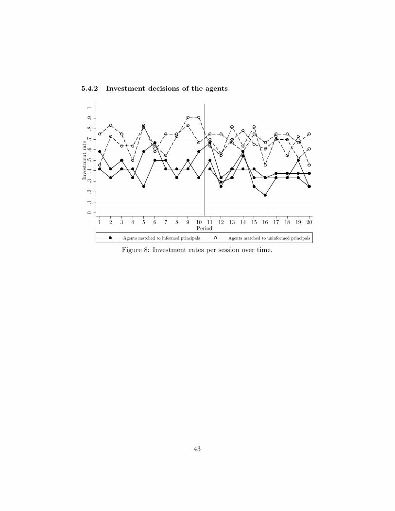
5.4.2 Investment decisions of the agents0

.1.2

.3.4

.5.6

.7.8

.91

Inves

tmen

t ra

te

1 2 3 4 5 6 7 8 9 10 11 12 13 14 15 16 17 18 19 20Period

Agents matched to informed principals Agents matched to uninformed principals

Figure 8: Investment rates per session over time.

43

Table 4: Propensity to invest conditional on treatment andsuccessful task completion.

Dependent variable Investment decision(Probit) (1-investment, 0-no investment)

(1) (2) (3)

Treatment −0.727∗∗∗ −0.754∗∗∗ −0.738∗∗∗

(1-informed) (0.205) (0.211) (0.221)

Success 0.429∗∗∗ 0.451∗∗∗

(1-task solved) (0.096) (0.126)

Treatment×Success −0.040(0.190)

Constant 0.467∗∗∗ 0.299∗∗ 0.291∗∗

(0.146) (0.149) (0.147)

N 1410 1410 1410R2 −916.436 −897.552 −897.512F 12.575 29.023 29.581

Note: Values in parentheses represent standard errors corrected for clus-ters on the individual level. Asterisks represent p-values: ∗p < 0.1,∗∗p < 0.05, ∗∗∗p < 0.01.

44

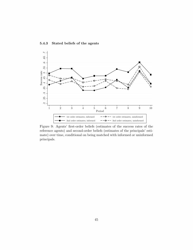
5.4.3 Stated beliefs of the agents.2

.25

.3.3

5.4

.45

.5.5

5.6

.65

.7Succ

ess

rate

1 2 3 4 5 6 7 8 9 10Period

1st order estimates, informed 1st order estimates, uninformed

2nd order estimates, informed 2nd order estimates, uninformed

Figure 9: Agents’ first-order beliefs (estimates of the success rates of thereference agents) and second-order beliefs (estimates of the principals’ esti-mate) over time, conditional on being matched with informed or uninformedprincipals.

45

0.0

0.1

0.2

0.3

0.4

0.5

0.6

0.7

0.8

0.9

1.0

Cum

ula

tive

dis

trib

uti

on funct

ion

-0.1 0.0 0.1 0.2 0.3

Average difference between second-order and first-order belief per agent

Agents matched touninformed principals

Agents matched toinformed principals

Figure 10: Empirical cumulative distribution functions of each agent’s av-erage difference between her second-order belief (estimate of the principal’sestimate of the success rate) and her first-order belief (own estimate of thesuccess rates), conditional on being matched with informed or uninformedprincipals.

Table 5 reports the results of regressions of average individual differencesbetween the agents’ second- and first-order beliefs on a constant, a treatmentdummy, a gender dummy, and individual risk attitudes as measured byDOSE. The treatment effect remains significant and becomes—if anything—somewhat larger when we add these controls. There is virtually no effect ofrisk attitude on the difference between agents’ first- and second-order beliefs(columns 4 and 5), and female agents in the uninformed treatment show asomewhat (but not significantly) larger gap between their own estimates ofthe success rate and their belief about the corresponding estimates of theprincipals (columns 3 and 5).

46

Table 5: Mean individual differences in second-order beliefs (estimate of the prin-cipal’s estimate) and first-order beliefs bA1,i (estimate of success rate) by treatmentand further controls.

Dependent variable (bA2,i − bA1,i) = T−1∑

t(bA2,i,t − bA1,i,t)

(OLS) (1) (2) (3) (4) (5)

Treatment 0.068∗∗∗ 0.067∗∗∗ 0.089∗∗∗ 0.073∗∗∗ 0.090∗∗∗

(1-informed) (0.019) (0.019) (0.024) (0.020) (0.024)

Gender 0.013 0.047 0.045(1-female) (0.020) (0.029) (0.030)

Treatment×Gender −0.062 −0.056(0.040) (0.041)

Coef. risk aversion −0.006 −0.004(DOSE) (0.006) (0.006)

Constant 0.044∗∗∗ 0.040∗∗ 0.030∗ 0.048∗∗∗ 0.034∗

(0.014) (0.015) (0.016) (0.014) (0.017)

N 47 47 47 47 47R2 0.220 0.228 0.270 0.236 0.278F 12.720 6.490 5.289 6.787 4.035

Note: Values in parentheses represent standard errors. Asterisk represent p-values: ∗p < 0.1,∗∗p < 0.05, ∗∗∗p < 0.01.

47

Table 6: Individual differences between second-orderbeliefs and first-order beliefs conditional on treatmentand successful task completion.

Dependent variable (bA2,t,i − bA1,t,i)

(OLS) (1) (2) (3)

Treatment 0.068∗∗∗ 0.068∗∗∗ 0.067∗∗∗

(1-informed) (0.019) (0.019) (0.024)

Success −0.039∗∗∗ −0.041∗∗

(1-task solved) (0.011) (0.017)

Treatment×Success 0.003(0.022)

Constant 0.044∗∗∗ 0.058∗∗∗ 0.058∗∗∗

(0.015) (0.017) (0.019)

N 470 470 470R2 0.090 0.117 0.117F 12.828 17.767 13.296

Note: Values in parentheses represent standard errors correctedfor clusters on the individual level. Asterisks represent p-values:∗p < 0.1, ∗∗p < 0.05, ∗∗∗p < 0.01.

48

5.5 Instructions

5.5.1 Instructions for principals (translated from German)

Welcome to the experiment!

The experiment that you will be participating in is part of a project fundedby the German Research Foundation (DFG). It aims to analyze economicdecision-making.

You are not allowed to use any electronic devices or to communicate withother participants during the experiment. You may only use programs andfeatures that are allocated to the experiment. Do not talk to any otherparticipant. Please raise your hand if you have any questions. We will thenapproach you and answer your question in private. Please do not under anycircumstances raise your voice while asking a question. Should the questionbe relevant for everyone, we will repeat it aloud and answer it. If you breakthese rules, we may have to exclude you from the experiment and fromreceiving payment.

You will receive a show-up fee of 5 Euros for your attendance. You can earnadditional money through the experiment. The level of your earnings de-pends on your decisions, the decisions of participants in former experiments,and on chance. The instructions are the same for everyone. A detailed planof procedures and the conditions of payment will be explained below.

Tasks

You will face 20 tasks in the course of the experiment. For each task, youwill be shown a short video. Each video consists of two images that areshown alternately. Your task is to spot the difference between the images.

The duration of each video is 14 seconds. After each video, you will have40 seconds to submit an answer. The interface will show a numbered gridtogether with the image containing the difference. To solve the task, enterone of the numbers corresponding to a field containing the difference. Ifthe difference is covered by more than one field, each field containing thedifference will be evaluated as a correct answer.

You will receive [Informed treatment: 0.30 Euros] [Uninformedtreatment: 0.50 Euros] for each task you solve correctly.

Estimates

49

Other participants in previous experiments performed all tasks you will facein this experiment. Like you, these previous performers also had to spot thedifference between the two images of each video.

After performing each task, you will have the opportunity to estimate thepercentage of previous performers that spotted the difference. Therefore,you will watch exactly the same videos as the previous performers. Theprevious performers also had 40 seconds to submit an answer, just like you,and were also paid according to their performance. [Informed treatmentonly: Before each video, you will receive a guide to the solution of the task.Please note that the previous performers did not receive solution guides.]

At the end of the experiment, the computer will randomly select two videos.Your estimates for these videos will be relevant for your payoff. For eachof the payoff-relevant videos, the following holds: If your estimate is withinthe interval +/– 5 percentage points around the true percentage of previousperformers that correctly identified the difference, you receive 12 Euros.

Consider the following example. Assume that for one of the two payoff-relevant videos, 50% of the previous performers correctly identified the dif-ference in this video. If you estimated that 53% of the previous performersspotted the difference, then you will receive 12 Euros. However, if you esti-mated that 57% of the previous performers spotted the difference, then youwill receive 0 Euros.

You will start with three practice videos to familiarize yourself with theprocedure. The practice rounds are not payoff relevant. Afterward, the 20payoff-relevant videos will follow.

Further procedure

After you submit your estimates for the 20 videos, you can earn money withadditional decision-making problems. Further details will be given duringthe experiment.

At the end of the experiment, we will ask you to fill in a questionnaire. Eventhough your answers will not affect your payoff, we kindly ask you to answerthe questions carefully.

After you completed the questionnaire, you will be informed about yourpayoff from performing the tasks, your payoff from your estimates, yourpayoff from the additional decision making problems, as well as your total

50

payoff in this experiment. Please remain seated until the experimenter letsyou know that you may collect your payment.

Do you have questions? If yes, please raise your hand. We will answer yourquestions in private.

Thank you for participating in this experiment!

51

Comprehension questions

1. How many (potentially payoff-relevant) videos will you evaluate intotal?

—————–

2. How many of these videos will be selected for payment regarding yourestimate of the previous performers?

—————–

3. What are the components of your total payoff?

—————–

4. Assume the computer randomly selected the following exemplaryvideos for payment regarding your estimates

Video a): 62% of the previous performers found the solution.

Video b): 35% of the previous performers found the solution.

What is your payoff from your estimates if you estimated that in videoa) 57% and in video b) 36% of the previous performers spotted thedifference?

—————–

5. What is your payoff from your estimates if you estimated that in videoa) 87% and in video b) 29% of the previous performers spotted thedifference?

—————–

52

5.5.2 Instructions for agents (translated from German)

Welcome to the experiment!

The experiment that you will be participating in is part of a project fundedby the German Research Foundation (DFG). It aims to analyze economicdecision-making.

You are not allowed to use any electronic devices or to communicate withother participants during the experiment. You may only use programs andfeatures that are allocated to the experiment. Do not talk to any otherparticipant. Please raise your hand if you have any questions. We will thenapproach you and answer your question in private. Please do not under anycircumstances raise your voice while asking a question. Should the questionbe relevant for everyone, we will repeat it aloud and answer it. If you breakthese rules, we may have to exclude you from the experiment and fromreceiving payment.

You will receive a show-up fee of 8 Euros for your attendance. You can earnadditional money through the experiment. The level of your earnings de-pends on your decisions, the decisions of participants in former experiments,and on chance. The instructions are the same for everyone. A detailed planof procedures and the conditions of payment will be explained below.

Tasks

You will face 20 tasks in the course of the experiment. For each task, youwill be shown a short video. Each video consists of two images that areshown alternately. Your task is to spot the difference between the images.

Figure 1 shows an example. Image A of the example shows a kayaker on theleft side. In image B, the kayaker is not present.

The duration of each video is 14 seconds. After each video, you will have40 seconds to submit an answer. The interface will show a numbered gridtogether with the image containing the difference (see Figure 2).

In each video, the difference between the images covers at least two fields.To solve the task, enter one of the grid numbers corresponding to a fieldcontaining the difference. That is, the number of any field containing thedifference will be evaluated as a correct answer.

53

Image A Image B

Figure 1: Example of an image pair. Image sequence in the experiment: A,B, A, B, . . . .

Figure 2: Response grid.

The experiment consists of 20 such tasks. The order of the tasks was ran-domly determined by the computer and is the same for all participants. Youwill receive 0.50 Euros for each task you solve correctly.

Previous participants

Performers

Participants in previous experiments performed all tasks you will face in thisexperiment. Like you, these previous performers had to spot the differencebetween the two images in each video. They were also paid according totheir performance.

Evaluators

54

The degree of difficulty of the tasks that have been performed by the previousperformers (and will be performed by you in this experiment) has beenevaluated by further participants of previous experiments.

These evaluators were shown the tasks in the same way as the previousperformers (and you), including the 40-seconds response time. After watch-ing a video, the evaluators estimated the fraction of previous performersthat solved this task correctly. The evaluators were paid according to theaccuracy of their estimates.

[Informed treatment only: In contrast to the previous performers (andyou), the evaluators received guides to the solution before each task. Theevaluators were informed that the previous performers did not receive solu-tion guides.]

At the beginning of the experiment, one of the evaluators will be randomlymatched to you.

Insurance decision

During the experiment, you can earn additional money through insurancedecisions. You will make one insurance decision after each task. At the endof the experiment, one of your insurance decisions will be randomly selectedfor payment.

Your endowment for each insurance decision is 10 Euros.

Not buying insurance

If you do not buy the insurance, your payoff depends on the following factors:

(1) the number of previous performers (percent) who solved the currenttask + 10 (percent),

(2) the number of previous performers (percent) who solved the currenttask in the evaluator’s estimation.

If (1) is at least as high as (2), you will keep your endowment of 10 Euros.

If (1) is smaller than (2), you will lose your endowment; that is, you willreceive 0 Euros.

55

In other words, if you do not buy the insurance, your payoff will be deter-mined as follows: You will keep your endowment of 10 Euros if the eval-uator’s estimate of the performance of the previous performers is correct,an underestimation, or an overestimation by not more than 10 percentagepoints. Otherwise, you will lose your endowment.

Buying insurance

You have the opportunity to insure against this risk. The insurance costs6 Euros. If you buy the insurance, you will receive your endowment minusthe cost of insurance, that is, 4 Euros.

Example 1

Assume that 50% of the previous performers actually solved the task. Inthe evaluator’s estimation, 60% of the previous performers solved the task.Of course, you will not learn these values during the experiment.

If you did not buy the insurance, you will keep your endowment, because50% + 10% ≥ 60% The payoff from your insurance decision will thereforebe 10 Euros.

If you bought the insurance, you will receive your endowment minus the costof insurance, that is, 4 Euros.

Example 2

Assume again that 50% of the previous performers actually solved the task.In the evaluator’s estimation, 20% of the previous performers solved thetask. As in the previous example, you will receive 10 Euros if you did notbuy the insurance and 4 Euros if you bought the insurance.

Example 3

Assume again that 50% of the previous performers actually solved the task.In the evaluator’s estimation, 70% of the previous performers solved the task.In this example, you will receive 0 Euros if you did not buy the insuranceand 4 Euros if, you bought the insurance.

Summary and further procedure

The experiment consists of 20 rounds in total. At the beginning of eachround, you will work on the task; that is, you will receive 0.50 Euros if youspot the difference between the two images in the video.

56

After each task, you can earn additional money through an insurance deci-sion. At the end of the experiment, one of your insurance decisions will berandomly selected for payment. Because you do not know which insurancedecision is selected for payment, you should treat each insurance decision asif it were payoff relevant.

After you make your insurance decision, you will receive feedback with aguide regarding the solution to the current task. [Informed treatment:The evaluators received the same guide before watching the task.] [Unin-formed treatment: The evaluators did not receive solution guides.]

You will start with five practice rounds to familiarize yourself with the pro-cedure. The practice rounds are not payoff relevant. Afterward, the 20payoff-relevant rounds will follow.

After the 20 rounds, you can earn money through additional decision-makingproblems. Further details will be given during the experiment.

At the end of the experiment, we will ask you to fill in a questionnaire. Eventhough your answers in this part will not affect your payoff, we kindly askyou to answer the questions carefully.

Do you have questions? If yes, please raise your hand. We will answer yourquestions in private.

Thank you for participating in this experiment!

Comprehension questions

1. When do you make your insurance decision—before or after youwatched the task?

2. Are the following statements true or false?

(a) The evaluators received a guide to the solution to each task.

(b) The evaluators did not receive guides to the solution to the tasks.

(c) The evaluators received a guide to the solution before watchingand evaluating the task.

(d) At the end of the experiment, one of my insurance decisions willbe randomly selected by the computer for payment.

57

(e) My payment at the end of the experiment consists of the show-upfee (8 Euros), the payoff from performing the tasks (0.50 Eurosper task solved), the payoff from one insurance decision, and thepayoff from further decision-making problems.

3. Assume the computer randomly selected videos for payment with thefollowing exemplary characteristics. Provide the payoff from your in-surance decision for each example.

Example a)

• 62% of the previous performers found the solution.

• The evaluator randomly matched to you estimated that 72%of the previous performers spotted the difference.

• You did not buy the insurance.

Example b)

• 62% of the previous performers found the solution.

• The evaluator randomly matched to you estimated that 75%of the previous performers spotted the difference.

• You did not buy the insurance.

Example c)

• 34% of the previous performers found the solution.

• The evaluator randomly matched to you estimated that 41%of the previous performers spotted the difference.

• You did not buy the insurance.

Example d)

• 34% of the previous performers found the solution.

• The evaluator randomly matched to you estimated that 30%of the previous performers spotted the difference.

• You did not buy the insurance.

4. Consider again the examples in 3. For each example, assume youdid not buy the insurance. What is your payoff from your insurancedecisions in each of the examples?

58