THE BERNOULLI OPERATOR - Linas · 2014-12-03 · This document explores the Bernoulli operator, ......
66
THE BERNOULLI OPERATOR LINAS VEPŠTAS <[email protected]> ABSTRACT. This document explores the Bernoulli operator, giving it a variety of different definitions. In one definition, it is the shift operator acting on infinite strings of binary digits. In another definition, it is the transfer operator (the Frobenius-Perron operator) of the Bernoulli map, also variously known as the doubling map or the sawtooth map. The map is interesting for multiple reasons. One is that the set of infinite binary strings is the Cantor set; this implies that the Bernoulli operator has a set of fractal eigenfunctions. These are given by the Takagi (or Blancmange) curve. The set of all infinite binary strings can also be understood as the infinite binary tree. This binary tree has a large number of self-similarities, given by the dyadic monoid. The dyadic monoid has an extension to the modular group PSL(2, Z), which plays an important role in analytic number theory; and so there are many connections between the Bernoulli map and various number-theoretic functions, including the Moebius function and the Riemann zeta function. The Bernoulli map has been studied as a shift operator, in the context of functional analysis [24]. More recently, it has been studied in the physics community as an exactly solvable model for chaotic dynamics and the entropy-increaing thermodynamic arrow of time[26, 14, 6]. Some of what is presented here is review material. New content includes a full devel- opment of the continuous spectrum of this operator, including a presentation of the fractal eigenfunctions, and how these span the same space as the the Hurwitz-zeta function eigen- functions. That is, both provide a basis for the operator, and the fractal basis is a linear combination of the smooth basis, and v.v. The connection to both classic and analytic number theory is also underscored. A simple proof that any totally multiplicative function is associated with a function obeying the multiplication theorem is provided. This document is meant to be read along with multiple companion papers which further expand the ties into number theory, and into fractal symmetries[30]. Most notable of these is that the shift operator acting on continued fractions gives the Gauss-Kuzmin-Wirising (GKW) operator[28]; the (iso-)morphism between the continued fractions and the real numbers given by the Minkowski Question Mark function[33, 29]. This, in turn, allows a novel reformulation of the Riemann Hypothesis as a bound on a rapdily-converging series representation for the Riemann zeta function[11, 31]. An effort is made to keep the presentation as simple as possible, making this document accesible to the general mathematical audience. This document is perennially in draft form, having multiple unfinished sections. It is occasionally updated with new results or clarifications. 1. THE BERNOULLI OPERATOR THIS IS A SET OF WORKING NOTES. It’s somewhat loosely structured, and some- times messy. The presentation alternates between easy, and advanced: many parts of this paper are readable by students with modest mathematical knowledge, while other sections presume and require expert familiarity. In general, the harder topics appear later in the text. The intro hasn’t been written yet; but if it was, it would explain why this is an interesting topic. In short, having a clear understanding of transfer operators is vital to the branches of physics concerned with dynamical systems and the arrow of time. The Bernoulli operator Date: 2 January 2004 (revised 2008, 2010, 30 November 2014). 1
Transcript of THE BERNOULLI OPERATOR - Linas · 2014-12-03 · This document explores the Bernoulli operator, ......

THE BERNOULLI OPERATOR
LINAS VEPŠTAS <[email protected]>
ABSTRACT. This document explores the Bernoulli operator, giving it a variety of differentdefinitions. In one definition, it is the shift operator acting on infinite strings of binarydigits. In another definition, it is the transfer operator (the Frobenius-Perron operator) ofthe Bernoulli map, also variously known as the doubling map or the sawtooth map.
The map is interesting for multiple reasons. One is that the set of infinite binary stringsis the Cantor set; this implies that the Bernoulli operator has a set of fractal eigenfunctions.These are given by the Takagi (or Blancmange) curve. The set of all infinite binary stringscan also be understood as the infinite binary tree. This binary tree has a large number ofself-similarities, given by the dyadic monoid. The dyadic monoid has an extension to themodular group PSL(2,Z), which plays an important role in analytic number theory; andso there are many connections between the Bernoulli map and various number-theoreticfunctions, including the Moebius function and the Riemann zeta function.
The Bernoulli map has been studied as a shift operator, in the context of functionalanalysis [24]. More recently, it has been studied in the physics community as an exactlysolvable model for chaotic dynamics and the entropy-increaing thermodynamic arrow oftime[26, 14, 6].
Some of what is presented here is review material. New content includes a full devel-opment of the continuous spectrum of this operator, including a presentation of the fractaleigenfunctions, and how these span the same space as the the Hurwitz-zeta function eigen-functions. That is, both provide a basis for the operator, and the fractal basis is a linearcombination of the smooth basis, and v.v. The connection to both classic and analyticnumber theory is also underscored. A simple proof that any totally multiplicative functionis associated with a function obeying the multiplication theorem is provided.
This document is meant to be read along with multiple companion papers which furtherexpand the ties into number theory, and into fractal symmetries[30]. Most notable of theseis that the shift operator acting on continued fractions gives the Gauss-Kuzmin-Wirising(GKW) operator[28]; the (iso-)morphism between the continued fractions and the realnumbers given by the Minkowski Question Mark function[33, 29]. This, in turn, allows anovel reformulation of the Riemann Hypothesis as a bound on a rapdily-converging seriesrepresentation for the Riemann zeta function[11, 31].
An effort is made to keep the presentation as simple as possible, making this documentaccesible to the general mathematical audience. This document is perennially in draftform, having multiple unfinished sections. It is occasionally updated with new results orclarifications.
1. THE BERNOULLI OPERATOR
THIS IS A SET OF WORKING NOTES. It’s somewhat loosely structured, and some-times messy. The presentation alternates between easy, and advanced: many parts of thispaper are readable by students with modest mathematical knowledge, while other sectionspresume and require expert familiarity. In general, the harder topics appear later in the text.
The intro hasn’t been written yet; but if it was, it would explain why this is an interestingtopic. In short, having a clear understanding of transfer operators is vital to the branches ofphysics concerned with dynamical systems and the arrow of time. The Bernoulli operator
Date: 2 January 2004 (revised 2008, 2010, 30 November 2014).1

THE BERNOULLI OPERATOR 2
just happens to be a particularly simple, exactly-solvable case. What is more, Hamltoniansystems very frequently have a repeller with a stucture that is the product of a Cantor setand a smooth manifold; the dynamics on the Cantor set part of the repeller is then isomor-phic to the Bernoulli shift. For example, Sinai’s billiards are isomorphic to a Bernoullishift [xxx need ref]. Geodesic flows on manifolds of negative curvature (Anosov flows)are also isomorphic to the Bernoulli shift [xxx need ref]. This wide applicability justifiesan exhaustive review of the topic.
General background material, laying a modern foundation for the study of chaotic dy-namical systems and statistical mechanics, can be found in Mackey[21] and Gaspard[15].Some recent general results for Frobenius-Perron and Koopman operators are given byDing[5]; see also references therein [xxx todo]. There are many earlier results on theBernoulli operator, which is known by many names; besides being called a “Bernoullishift” or “Bernoulli scheme”, it is sometimes more prosaically refered to as a “expandingmap of the circle”. Kolmogorov and Sinai introduced entropy as a means for determin-ing isomorphic shifts[1958, need ref]. Rochberg studies it as a shift operator[24]. Orn-stein[need ref, in V.I. Arnold, A. Avez, "Ergodic problems of classical mechanics" , Ben-jamin (1968)] provides an isomorphism proof, showing when two different Bernoulli shiftsare isomorphic to one-another. Ruelle studies it as a prototype for Axiom A systems[26].Gaspard provides the Bernoulli polynomial solutions[14]. Driebe shows how it is conju-gate to a broad class of maps, and pursues generalizations[6].
The layout is roughly as following (xxx this summary needs work)
• Define the Bernoulli operator, demonstrate some of its eigenfunctions and eigen-values. The presentation is a simplified variant of the material in [6], generalizedto p-adic definitions.
• Present the Hurwitz Zeta and fractal eigenfunctions; show that these are just linearcombinations of one-another, and span the same space. Notable is the fact that thefractal eigenfunctions are not differentiable on the rational numbers, whereas theHurwitz Zeta eigenvalues are classically differentiable almost everywhere.
• Present a more abstract, but more firm/well-founded foundation for the earlier re-sults. The more abstract formulation is in terms of the Cantor set. Here, we takethe Cantor set to be the Cartesian product 2ω = 2× 2× ·· · of a countably infi-nite number ω of copies of the set 2 = 0,1. That is, we take the Cantor setto be the set of all infinitely long strings of binary digits, taken with the prod-uct topology. Of course, strings of binary digits can represent the real numbers;but the Cantor set differs from the real numbers in that, unlike the reals, one has0.111 · · · 6= 1.000 · · · . This foundation can then lead to deeper results, as well asshed light on some of the more confusing/paradoxical results that arise in the in-formal treatment.
• Show that the Perron-Frobenius operator is the measure-theoretic pullback. Thisis a nice, formal, category-theoretic way of defining the FP transfer operator.
Some of the sections, including the sections on orthogonality and completeness, are insuf-ficiently rigorous, and could be tightened up a good bit.
Some new results that are general (and not related to Bernoulli) are presented here:
• The paragraph following 8.6 which generalizes the Wold decomposition 7.2, andshows how to build eigenfunctions, in general, for any transfer operator on anyCartesian product space. (It would be nice to reconcile this with the results ofDing[5] as to the domain of the spectrum (a disk, for L1spaces, which are the most

THE BERNOULLI OPERATOR 3
frequently studied). Now, one of the recurring themes in this set of papers is self-similarity and scaling behavior; such self-similarity will always hold, in general,on uniform Cartesian products; and so many new, general facts could be easilystated here as well.
• The results of section 10 are entirely new, as far as I know, and provide a muchclearer vocabulary (to me, at least) with which to talk about transfer operators.
Some new results that are specific to the Bernoulli operator:
• The presentation of the Hurwitz zeta eigenfunctions, of section 7.3, I believe arenew and have never been reported before. Notable is that these are well-definedfor eigenvalues lying outside of the unit disk |λ | ≤ 1; in fact, these are well-definedfor any complex λ . This in no way contradicts general results that the spectrum ofFrobenius-Perron operators lies in the unit disk when one considers eigenfunctionsthat lie in L1. These eigenfunctions are analytic; they are just not integrable overthe entire unit interval. This simply shows: there is more to life than just thespectrum inside the unit disk.
• The presentation of the fractal eigenfunctions, of section 8.1, are new; the obser-vation that these are self-similar and have a scaling behavior is new.
2. INTRODUCTION
The method of the transfer operator was introduced by David Ruelle[26][verify ref] asa powerful mechanism for studying the nature of iterated maps. Before this, iterated func-tions were typically studied by looking at the trajectories of sets of points. This approach,though obvious, has disadvantages for both the disciplines of physics (e.g. loss of differ-entiability) and mathematics (e.g. non-measurable sets, axiom of choice). The transferoperator, sometimes called the Perron-Frobenius operator, or the Ruelle-Frobenius-Perronoperator, provides a different, stronger setting, by making incorporating the topology ofthe space that the map acts on. This section provides a gentle introduction to the concept.
In general, an iterated function g : X → X maps a space X to itself. When studying aniterated function, one often asks about the orbits of points: Are there fixed points, attractorsor repellors, or saddle points? Is the action of g may be ergodic or chaotic? Endowing theset X with a topology (for the unit interval, the natural topology on the reals), one typicallyasks if g is strong or weak mixing, or merely topologically mixing. The above questionsmay all be grouped under a heading: ’the study of iterated operators by means of point settopology’. A change in perspective is gained by introducing a measure on the space X .This radically alters how g can be discussed.
Consider how g acts on distributions, rather than points. Suppose the space X is theunit interval [0,1]. Intuitively, consider a dusting of points on the unit interval, with a localdensity given by ρ(x) at point x ∈ [0,1], and then consider how this dusting or densityevolves upon iteration by g. This verbal description may be given form as
(2.1) ρ′(y) =
∫ 1
0δ (y−g(x))ρ(x) dx
where ρ ′(y) is the new density at point y = g(x) and δ is the Dirac delta function. In thisviewpoint, g becomes an operator that maps densities ρ to other densities ρ ′, or notation-ally,
Lgρ = ρ′

THE BERNOULLI OPERATOR 4
The operator Lg is called the transfer operator or the Ruelle-Frobenius-Perron operator. Itis a linear operator, for clearly
Lg(aρ1 +bρ2) = aLgρ1 +bLgρ2
for constants a,b and densities ρ1,ρ2.Although the word “density” implies that ρ is a smooth map from the unit interval to
the non-negative reals, there is no particular need to enforce this. The function ρ may be amap from the unit interval to any ring R, and it need not be smooth, differentiable or evencontinuous. Usually, we’ll take the ring R to the reals R, but in fact, it could be any ring orfield. Thus, Lg is an operator that maps functions on the unit interval to other functions onthe unit interval:
Lg : F [0,1]→F [0,1]with ρ ∈F [0,1]. The precise properties of Lg depend strongly on what, exactly, is takento be “the set of functions F [0,1] on the unit interval”. An exploration of the differentspaces makes up much of the content of this paper. There are many spaces to choosefrom: the space of polynomials, the space of square-integrable functions, or possibly yetother spaces. In general, the properties of Lg depend on the topology given to F . Mostgenerally, Lg is an operator acting on a topological space endowed with multiplication andaddition, that is, a topological vector space.
The definition of eqn 2.1, for a general space X , requires the definition of an integral onX , and the definition of the Dirac delta function. This is in general possible only when Xis endowed with a measure and the associated Borel sigma algebra. The space F [X ] thenmust be a space of of measurable, sigma-additive functions, if eqn 2.1 is to be meaningful.Given this setting, the transfer operator turns out to be one and the same as the push-forward of g on the set of measurable, sigma-additive functions. A formalization and proofof this is given in a much later section. For most of what follows, though, these formalitiescan be avoided.
When the function g is differentiable, and doesn’t have a vanishing derivative, the trans-fer operator can be defined as
(2.2) [Lgρ] (y) = ∑x:y=g(x)
ρ(x)|dg(x)/dx|
where the sum is presumed to extend over at most a countable number of points. It is notat all hard to show that, for a “reasonable” class of differentiable functions, that 2.1 and2.2 are equivalent definitions.
Because Lg is a linear operator, all of the usual language of operator theory may bebrought to bear on its study. As a start, one looks for its representations and the eigenvec-tors and eigenspaces associated with each representation. It is typically pertinent to discussany symmetries and isomorphisms these spaces might have. Thus, for example, if Lg isa compact operator, then it’s spectrum is constrained by well-known theorems[need ref]:the spectrum is discrete, countable, bounded, and, if infinite, has an accumulation pointat zero. It is from here whence the transfer operator gets the name ’Perron-Frobenius’:insofar as compact operators are ’a lot like’ finite matrices, the Perron-Frobenius theoremapplies. So, for example, if one chooses the space F [X ] to be the space of polynomialson X , then, for many ’reasonable’ g, the operator Lg is compact. After we narrow the dis-cussion to the Bernoulli operator, we will find that this is exactly the case. Alternately, onemay choose F [X ] to be a Banach space, or possibly a Hilbert space of square-integrablefunctions on X . In this case, it turns out that, for many ’reasonable’ g, that the conjugate ofLg is and isometry and specifically, a shift operator. In this case, it is well-known from the

THE BERNOULLI OPERATOR 5
Wold-von Neumann decomposition that the spectrum of Lg fills the entire unit disk on thecomplex plane. We’ll provide several constructions for the Bernoulli operator that exhibitthis (and more; a spectrum that fills the entire complex plane!).
The composition operator Cg : F [X ]→F [X ] acts on functions and is defined as Cg f =f g. It is the right-inverse to Lg but usually not the left inverse: LgCg is the identity, butCgLg is not, in general. In physics, the composition operator is known as the Koopmanoperator[19]. In mathematics, the AMS category 47B33 is used to classify articles pertain-ing to the study of composition operators.
Both operators have physical significance, and occur frequently in the study of dynam-ical systems and statistical mechanics. For example, Ruelle has shown that the Fourriertransform of the correlation function for Axiom A dynamical systems is meromorphic ona strip[27]; the poles of the correlation function are now called Ruelle reosnances, and canbe shown to correspond to the logarithm of the eigenvalues of the transfer operator. Inparticular, this is where the term “transfer operator” comes from: in spin-lattice systems,the transfer matrix simply describes how nearest-neighbor states are connected. When theinteraction is long-range, the matrix becomes infinite-dimensional, and thus an operator.That it also typically happens to satisfy the provisions of the Frobenius-Perron theoremis where the name ’Frobenius-Perron operator comes from. Other physically significantconstructions follow, including the resolvant, the Fredholm determinant and the dynamicalzeta function.
The Cantor set, and more generally, the product topology on infinite Cartesian products,plays a special role in what follows. This is in part due to the nature of shift operators andthe Wold decomposition, but can be considered a generalization. To keep things simple,consider the unit interval. For any x ∈ [0,1], one may write the decimal expansion for x:
x = 0.d1d2d3 · · ·=∞
∑n=1
dn10−n
where dn is the n’th decimal digit of x. The space of all such decimal expansions is theCartesian product D×D×D×·· · where D is the finite set D= 0,1,2,3, · · · ,9. Althoughthis is ’obvious’, it is not commonly appreciated that this infinite Cartesian product is theCantor set. This has practical implications for the study of transfer operators: one maychoose to work with not only the ’natural’ topology on the unit interval, but also withthe Cantor set topology (aka the product topology or ’cylinder set’ topology). This canhave a subtle effect on the space of measurable functions F [X ], and can, as well, openup new ways of thinking about the problem, thus offering additional tools, techniques andtheorems.
To be more precise, one considers the unit interval [0,1] to consist of the set of strings
Ω =
σ = (σ0,σ1,σ2, . . .) : σk ∈ 0,1, . . . , p−1 , x =
∞
∑k=0
σk p−(k+1) , x ∈ [0,1]
Intuitively, this set is simply the set of all the digits of a base-p expansion of the real num-bers x ∈ [0,1]. That one may consider a shift operator on this space is now intuitivelyobvious; that this shift operator has anything at all to do with that of the Wold decompo-sition is less so. This connection will be explored in greater detail in this text. This spaceis equivalent to the collection of all field configurations of a one-dimensional, one-sidedlattice, where each lattice location can take on one of p values. In physics, such lattices arecalled ’spin lattices’ or ’spin networks’; this cross-over of concepts provides another wayof gaining insight.

THE BERNOULLI OPERATOR 6
A few more remarks remain in order. The space Ω may be endowed with one of twodifferent metrics: the natural metric, the closure of which leads to the natural topology onthe real numbers, and the p-adic metric, whose closure gives the p-adic numbers. Theseare important to the study of finite function fields and p-adic analysis in general. Althoughthis can be quite interesting, this text does not currently deal any further with the p-adicmetric or the resulting closure.
The real numbers also have yet another product representation. By considering Ω =N×N×·· · , one has sequences of positive integers that may be interpreted as a continuedfraction:
x = [0;σ1,σ2,σ3, . . .] =1
σ1 +1
σ2+1
σ3+...
The measure on this product space is radically different than the usual measure, and isconsiderably harder to study; it is the Minkowski measure, the derivative of the Minkowskiquestion-mark function. An introduction to lattice models, the product topology, and theirapplications to the study of transfer operators for continued fractions may be found in[23]. Another exploration with certain specific results can be found in [33]. The continuedfraction will not be further addressed in this text; see instead [28] for a detailed treatment.
XXX ToDo: in order for the Perron-Frobenius thm to apply, we must show that Lg isnon-negative; we have not done so yet.
3. TRANSFER OPERATOR OF THE BERNOULLI MAP
The Bernoulli map is important in physics as an exactly solvable example of determin-istic chaos, and, in particular, as a model of symbolic dynamics on Axiom A dynamicalsystems[26, 14, 6]. A purely mathematical treatment of the operator, considered as a shiftoperator on Hilbert space, is given in [24]. This and the next section recaps those resultsusing a simplified development and simpler tools. The simplified development enables thediscussion of more complex scenarios, given in later sections.
The Bernoulli map is given by
(3.1) b(x) = 2x−b2xc
where bxc denotes the integer part of x. The map can be thought of as popping the leadingdigit off of the binary or 2-adic expansion of x. This map has a positive Lyapunov exponentand is highly chaotic, as, in a certain sense, one can say that the digits of the binary ex-pansion of some ’arbitrary’ number are ’unpredictable’, and that the orbits of two close-bynumbers will eventually become ’uncorrelated’ (after suitably defining what we mean by’arbitrary’ and ’unpredictable’). Closely related is the p-adic map, given by
a(x) = px−bpxc
for p an integer. As above, this map has the effect of popping off the leading digit of thebase-p expansion of x. In a similar vein, one may also consider the Gauss map
g(x) =1x−⌊
1x
⌋which has the effect of lopping of the leading digit of the continued fraction expansionof x. What these three maps have in common is that they deal with different (and, in acertain sense, inequivalent) representations of the continuum of real numbers. Each map ischaotic, but in a different way.

THE BERNOULLI OPERATOR 7
The Ruelle-Frobenius-Perron operator or transfer operator of the Bernoulli map is givenby
(3.2) [LB f ] (x) =12
[f( x
2
)+ f
(x+1
2
)]which follows directly from equation 2.2. Similarly, the transfer operator for the generalp-adic map is
(3.3) [Lp f ] (x) =1p
p−1
∑k=0
f(
x+ kp
)while that for the Gauss map is
[LG f ] (x) =∞
∑k=1
1(x+ k)2 f
(1
1+ x
)This last is known as the Gauss-Kuzmin-Wirsing operator[28, 23, 12, 10]. It is not studiedfurther here, although it has bearing on some results, due to its relationship to the repre-sentation of the real numbers.
One suggestive aspect of eqn Transfer Operator of the Bernoulli Map is that it takes thesuggestive form of the ’multiplication theorem’ (see wikipedia).
The Bernoulli operators commute: LpLq = LqLp and are multiplicative: LpLq =Lpq. The last property suggests that it is “sufficient” to work with prime p.
As noted above, the properties of the operator LB depend on the function space onwhich it acts, and the topology to be used on the unit interval. In particular, the spectrumof eigenvalues and eigenvectors for LB can vary from being discrete, to being continuous,depending on the the function space and topology. The simplest case assumes the naturaltopology of the reals on the unit interval, and takes as the function space the set of orthog-onal polynomials on the unit interval. In this case, the eigenfunctions may be shown to bethe Bernoulli polynomials Bn(x), associated with the eigenvalues 2−n. That is, one findsthat
[LBBn] (x) =12n Bn(x)
where the first few Bn(x) are
B0(x) =1
B1(x) =x− 12
B2(x) =x2− x+16
B3(x) =x3− 3x2
2+
x2
and so on. Perhaps the easiest proof that these are the eigenfunctions may be obtained byconsidering the generating function for the Bernoulli polynomials:
G(x, t) =text
et −1=
∞
∑n=0
Bn(x)tn
n!
It is then straight-forward to verify that
[LBG] (x, t) =12
[G( x
2, t)+G
(x+1
2, t)]
= G(
x,t2
)

THE BERNOULLI OPERATOR 8
or equivalently, by applying the linearity of LB, that
[LBG] (x, t) =∞
∑n=0
tn
n![LBBn] (x) =
∞
∑n=0
( t2
)n Bn(x)n!
and then equating the coefficients of the powers of t. This derivation follows for the generalp-adic case[14]:
Theorem. The eigenvalues of the p-adic transfer operator are the Bernoulli polynomials,and are associated with the eigenvalues p−n. That is, one has
[LpBn] (x) =1pn Bn(x)
Proof. The proof proceeds as in the above 2-adic case, and hinges on the factorization
wp−1 = (w−1)(wp−1 +wp−2 + · · ·+1
)Here, take wp−1 = et −1, so that
[LpG] (x, t) =1p
p−1
∑k=0
G(
x+ kp
, t)
=1p
tet −1
p−1
∑k=0
exp((x+ k)t
p
)
=tp
(1+ et/p + e2t/p + · · ·+ e(p−1)t/p
)et −1
= G(
x,tp
)Then, equating coefficients of powers of t of the generating function, one obtains the de-sired result.
The above theorem is a fancy restatement of an old and well-known result on theBernoulli polynomials, namely, the so-called “multiplication theorem” given by JosephLudwig Raabe in 1851[need ref] (see wikipedia). This is usually given in the more prosaicform of
Bn(px) = pn−1p−1
∑k=0
Bn
(x+
kp
)but amounts to the same thing. Curiously, multiplication theorems exist not only for theBernoulli polynomials, but more broadly, including the Gamma function and the Hurwitzzeta function. A later section will give a more general set of eigenfunctions in terms ofthe Hurwitz zeta. Several other connections to number theory are worth pointing out.Sums of the above kind are not atypical in the study of automorphic and modular forms;indeed, the Hecke operator[2] of number theory is essentially the sum of the Bernoullioperator and its transpose. This is perhaps not accidental: later sections will constructfractal eigenfunctions of Lp that have self-similarity under the dyadic monoid, which isa certain subset of the modular group. The mathematician’s word “automorphic” is asynonym for the physicist’s “self-similar”.
The following sections provide a more abstract and belabored derivation of the above re-sult. The goal of the abstraction is to develop the machinery needed to explore the Bernoullioperator in more general topological settings. Rather than starting with the Hilbert spaceof orthogonal polynomials on the unit interval, the next section defines a Banach space on

THE BERNOULLI OPERATOR 9
monomials, and its dual. The subsequent section then exposes the matrix elements of theBernoulli operator in this space.
4. THE POLYNOMIAL REPRESENTATION
The reason for working with polynomials is that they provide a convenient way of work-ing with infinitely-differentiable functions. A polynomial, with a finite number of terms, isinherently bounded on the unit interval. This is not generally the case when working witha square-integrable Hilbert space; square-integrable functions can be badly discontinuous,nor are they, in general, bounded. The hand-waving physics behind this is that “nature issmooth”, and so, insofar as the operator is a model for some natural physical process, onewants to stick to smooth functions. As will be seen, this has a tremendous effect on thespectrum of the operator.
The polynomial eigenvectors of the Bernoulli operator can be derived in several ways.One seemingly reasonable initial approach is to start with a Hilbert space of orthogonalpolynomials on the unit interval. This approach is taken by Driebe[6], who starts withthe Legendre polynomials, rescaled to the unit interval, and obtains the resulting Bernoullieigenvectors. This allows for a derivation of the right eigenvectors, but is then discoveredto generate difficulties when considering the left eigenvectors. This arises because thethe Bernoulli operator is not invertible in this Hilbert space: it is quite singular, in that[LB f ] = 0 whenever f is skew about 1/2, that is, whenever f (y) =− f (1/2+ y). A set ofleft eigenvectors can be found, but these are not polynomials or even ordinary real-valuedfunctions; rather, they are generalized functions, expressed as derivatives of the Dirac deltafunction. In essence, a “singular value decomposition” is thus performed on the Bernoullioperator, but, as the operator is not ’nice’ or ’symmetric’ in any common sense, the leftand right factors don’t have any particular structure or relation to one-another. From thisexercise, one concludes that starting with a Hilbert space of orthogonal polynomials offersno particular benefit.
Generalized functions are linear functionals from a space of functions to the reals. Thatis, generalized functions belong to the dual space of a function space. Given that theleft eigenvectors of the Bernoulli operator are “naturally” found to belong to such a dualspace (but only after laborious calculation, as in [6]), it then makes sense to work withthese, from the start. Thus, for the following, an infinite-dimensional vector space willbe constructed, with the basis elements being the monomials. The generalized functionsappear naturally as elements of the dual space. The transfer operator then has a clear andsimple representation in this space. In principle, this infinite-dimensional vector spacemay be taken to be a Banach space; however, the development below does not make anyparticular use of the norm that Banach spaces are equipped with.
Consider an infinite-dimensional vector space V with a countable ordered set of linearlyindependent basis vectors ek labelled by the natural numbers k. A general element v ∈ Vmay be written as v = ∑
∞k=0 akek. The dual space V ∗ is the set of all linear functionals
L : V → R. General elements of the dual space may be written as linear combinations ofthe basis elements e∗k , which are the maps such that e∗j(ek) = δ jk.
For the space P of real-analytic functions on the unit interval, there are many choicesone could make for the basis vectors. Most obviously, basis elements may be taken to bethe monomials ek = xk, so that a general real-analytic function f ∈P is written as
(4.1) f (x) =∞
∑n=0
anxn

THE BERNOULLI OPERATOR 10
This may be trivially interpreted as nothing more than the Taylor’s series for a real-valuedfunction expanded at x = 0. Other possibilities for basis vectors will be considered later.
The correct formalism for discussing the dual space is a bit trickier. Formally, elementsof the dual space are called 1-forms or differentials. Following historical convention, thelinear functionals of the dual space may be represented as integrals. That is, the linearfunctional L : P → R may be written as the integral
∫ 1
0l(x) f (x)dx
where f ∈P and l is some “generalized function” or “Schwarz function”, such as theDirac delta function. The difficulty with this is, of course, that “generalized functions”are not, in general, differentiable and can have other surprising properties. However, withcare, these can be handled in a consistent manner; a quick review follows, as such use isnot uncommon. The dual vectors may be written as
e∗k =(−1)k
k!δ(k)(x)
where δ (x) is the Dirac delta function. Thus, one has as the duality relation
(4.2) e∗j (ek) =∫ 1
0xk (−1) j
j!δ( j)(x)dx =
∫ 1
0δ (x)
d jxk
dx j dx = δ jk
after integration by parts. The relation 4.2 above demonstrates orthogonality; one may alsoshow completeness:
(4.3)∞
∑n=0
en⊗ e∗n =∞
∑n=0
xn (−1)n
n!δ(n)(y) = δ (x− y)
in that f (x) =∫
δ (x− y) f (y)dy whenever f is expressible as an analytic function.Another common notation is that of quantum mechanical bra-ket or Dirac notation.
Here, we write |n〉 = en and 〈n| = e∗n. The orthogonality condition becomes 〈n| m〉 = δnmwhile for completeness one writes
(4.4) I=∞
∑n=0
en⊗ e∗n =∞
∑n=0|n〉〈n|
The re-introduction of the coordinate x is done by writing 〈x| m〉= xm, while for the trans-pose one writes 〈n| x〉 = (−1)nδ (n)(x)/n!. The advantage of the bra-ket notation over theuse of the ek is that it can be used to make clear when one is discussing the coordinaterepresentation, involving x or δ (x), and when one is discussing the vector space elementsin the abstract, without reference to the coordinate representation. To fully articulate this

THE BERNOULLI OPERATOR 11
notation, one may write the Taylor’s series as
f (x) = 〈x| f 〉
=∞
∑n=0〈x|n〉〈n| f 〉
=∞
∑n=0
xn 〈n| f 〉
=∞
∑n=0
xn∫
dy〈n|y〉〈y| f 〉
=∞
∑n=0
xn∫
dy(−)n δ (n)(y)n!
f (y)
=∞
∑n=0
xn f (n)(0)n!
(4.5)
This notation allows the matrix elements Umn = 〈m |L |n〉 of the transfer operator to bearticulated as well. Starting with the matrix notation of equation 4.1, one has
[L f ] (x) =∞
∑m=0
bmxm =∞
∑m=0
xm∞
∑n=0
Umnan
or, equivalently
[L f ] (x) = 〈x |L f 〉=∞
∑m=0〈x |m 〉〈m |L f 〉=
∞
∑m=0
∞
∑n=0〈x |m 〉〈m |L |n〉〈n| f 〉
where 〈n| f 〉 = an and 〈n |L f 〉 = bn. Equating each power of xm one finds, in the matrixnotation, that
1m!
dm [L f ] (x)dxm
∣∣∣∣x=0
=∞
∑n=0
Umn1n!
dn f (x)dxn
∣∣∣∣x=0
where
〈n| f 〉= an =1n!
dn f (x)dxn
∣∣∣∣x=0
and so on. The formulation of the transfer operator given in equation 2.1 fits in this frame-work as well; it is merely the spatial representation of the matrix elements:
δ (x−g(y)) = L (x,y)
= 〈x |L |y〉=∞
∑m=0
∞
∑n=0〈x|m〉〈m |L |n〉〈n|y〉
So far, we’ve avoided discussions of convergence and completeness; these will be re-turned to shortly. Armed with these three different styles of notation, we can explore thematrix elements of the Bernoulli operator in this polynomial basis.
5. THE BERNOULLI OPERATOR IN THE POLYNOMIAL BASIS
This section reviews the structure of the Bernoulli operator LB in the polynomial basisdeveloped above. The matrix elements in the monomial basis are given by
(5.1) [LB]mk ≡Umk ≡ 〈m|U |k〉=δmk
2m +
(km
)Θmk
2k+1

THE BERNOULLI OPERATOR 12
where(
mk
)= m!
k!(m−k)! is the binomial coefficient, and
Θmk =
0 if k ≤ m1 if k > m
is a traceless, pure upper-triangular matrix. These matrix elements are easily obtained bydirect substitution, that is, by contemplating the coefficient to the xm term in the expansionof [
LBxk]=
12
[( x2
)k+
(1+ x
2
)k]
Both the diagonal elements, and the reason for the appearance of the binomial coefficientsshould be immediately clear. Note that the evaluation of these matrix elements does notrequire the evaluation of any sums with an infinite number of non-zero terms; the sums areall finite.
The eigenvalues may be promptly read off the diagonal; these eigenvalues are λn =2−n. Because the matrix is upper-triangular, it is easily solvable for both the left and righteigenvectors, which agree perfectly with those given by Driebe[6]. Visually, the upper-leftof this matrix looks like
Umk =
1 14
18
116
132 ...
0 12
14
316
18
0 0 14
316
316
0 0 0 18
18
0 0 0 0 116
... ...
The right and left eigenvectors are developed in the following sections. Note that Umk isvery well-behaved: all entries remain small. For large k, each column resembles a Gaussian(this follows from Stirling’s approximation for the factorial), and specifically, this Gaussianhas a peak at k = 2m. That is, one has Umk ≤Um,2m ≈ 1/2
√πm for large m.
5.1. Right eigenvectors. The right eigenvectors are denoted by |Bn〉 and have the vectorcomponents
(5.2) 〈k |Bn 〉=(
nk
)(1−Θn,k
)Bn−k =
(
nk
)Bn−k for k ≤ n
0 for k > n
where Bk are the Bernoulli numbers. Note that only a finite number of these vector com-ponents are non-vanishing.
Theorem. The |Bn〉 are eigenvectors of Umk, associated with eigenvalues 2−n. That is,
LB |Bn〉=12n |Bn〉

THE BERNOULLI OPERATOR 13
Proof. This may be verified in the monomial basis through brute-force multiplication ofthe vector into the matrix:
∞
∑k=0〈m|U |k〉〈k |Bn 〉 =
n
∑k=m
[δmk
2m +
(km
)Θmk
2k+1
](nk
)Bn−k
=1
2m
(nm
)Bn−m + ...non− trivial− taylor− expn
=12n 〈m |Bn 〉
XXX To-do: fill in details. Note that this proof does not require the evaluation of any sumswith an infinite number of non-zero elements; all sums are finite.
The right eigenvectors can be given a representation in coordinate space, and these arefound to be the Bernoulli polynomials discussed previously:
∞
∑k=0〈x|k〉〈k |Bn 〉=
n
∑k=0
(nk
)Bn−kxk = Bn(x)
These were previously shown to be eigenvectors, and so this is consistent with the above.One may conclude that the coordinate representation and the matrix representation for thistransfer operator are consistent.
5.2. Left Eigenvectors. This matrix expression for Umn also admits left eigenvectors whichcan be given an explicit representation. Letting the left eigenvectors be denoted by
⟨Bn∣∣,
they have, for n > 0, the components
(5.3)⟨
Bn∣∣k⟩= ( k
n−1
)1n(δnk +Θnk)
The zeroth left eigenvector is a special-case; it has components⟨
B0∣∣k⟩ = 1/(k+1). Un-
like the right eigenvectors, the left eigenvectors all have an infinite number of non-zerocomponents. They share the same eigenvalue spectrum with the right eigenvectors, so that
∞
∑k=0
⟨Bn∣∣m⟩Umk =
12n
⟨Bn∣∣k⟩
This may again be demonstrated by a brute-force evaluation of the sum. Despite the factthat an infinite number of the left eigenvector components are non-vanishing, this sum willonly contain a finite number of non-zero terms, and thus its finiteness is guaranteed onalgebraic grounds.
One may write down a coordinate-space representation for the left eigenvectors, bycontracting them against the dual-space basis elements 〈k|x〉. This leads directly to thegeneralized functions:⟨
Bn|x⟩
=∞
∑k=0
⟨Bn∣∣k⟩〈k|x〉
=∞
∑k=0
⟨Bn∣∣k⟩(−)k δ (k)(x)
k!
=1n
∞
∑k=n
(k
n−1
)(−)k δ (k)(x)
k!
=(−1)n+1
n!
[δ(n−1)(1− x)−δ
(n−1)(x)]
(5.4)

THE BERNOULLI OPERATOR 14
for the n > 0 case. The n = 0 left eigenvector is best understood by integrating it over somearbitrary function f (x):
∫ 1
0dx⟨
B0∣∣x⟩ f (x) =
∫ 1
0dx f (x)
∞
∑k=0
(−)k δ (k)(x)(k+1)!
=∞
∑k=0
f (k)(0)(k+1)!
=∞
∑k=0
f (k)(0)k!
∫ 1
0xkdx
=∫ 1
0f (x)dx
=⟨
B0∣∣ f⟩
The other left eigenvectors can also be made more concrete by looking at how they act onsome function f (x); this may be written as
(5.5)⟨
Bn∣∣ f⟩=
1n!
[f (n−1)(1)− f (n−1)(0)
]
5.3. Duality. That the left eigenvectors are dual to the Bernoulli polynomials, which canbe verified in either the matrix-element basis, or the coordinate-space representation.
Theorem. The left and right eigenvectors are dual, in that
⟨Bn∣∣Bm
⟩=
∞
∑k=0
⟨Bn∣∣k⟩〈k |Bm 〉= δnm
and furthermore, the duality is algebraic, in that no infinite sums need be performed todemonstrate duality.
Proof. Consider first the n = 0 case. One has
⟨B0∣∣Bm
⟩=
∞
∑k=0
⟨B0∣∣k⟩〈k |Bm 〉
=m
∑k=0
1k+1
(mk
)Bm−k
=1
m+1
m
∑j=0
(m+1
j
)B j
= δm0
where the substitution j = m− k was made to obtain the last sum. The vanishing of thelast sum is a well-known identity on the Bernoulli numbers. The n 6= 0 case requires more

THE BERNOULLI OPERATOR 15
work, but ends similarly:⟨Bn∣∣Bm
⟩=
∞
∑k=0
⟨Bn∣∣k⟩〈k |Bm 〉
=m
∑k=0
(k
n−1
)1n(δnk +Θnk)
(mk
)Bm−k
=1n
(n
n−1
)(mn
)Bm−n +
m
∑k=n+1
(k
n−1
)1n
(mk
)Bm−k
=
0 for n > mB0 for n = m(
mn
)Bm−n +
m!n!(m−n+1)! ∑
mk=n+1
(m−n+1
m− k
)Bm−k for n < m
The last case can be shown to vanish, by again making the substitution j = m− k, to get(mn
)Bm−n +
m!n!(m−n+1)!
m−n−1
∑j=0
(m−n+1
j
)B j
=m!
n!(m−n+1)!
m−n
∑j=0
(m−n+1
j
)B j = 0
thus concluding the proof. Notice that this proof does not require the evaluation of anyinfinite sums: all sums are performed over a finite number of terms.
This proof of duality may also be conducted in coordinate space, where it takes the form⟨Bn∣∣Bm
⟩=
∫ 1
0
⟨Bn∣∣x⟩〈x |Bm 〉 dx
=∫ 1
0
(−1)n+1
n!
[δ(n−1)(1− x)−δ
(n−1)(x)]
Bm(x)dx
=
0 for m < n−1
m!n!(m−n+1)! [Bm−n+1(1)−Bm−n+1(0)] for m≥ n−1
= δmn(5.6)
and so, as with most of the previous results, one may be lulled into a sense of complacencyabout the equivalence of the coordinate-space and monomial-vector-space representations.This complacency is ill-founded, as demonstrated below.
5.4. Completeness. Given this duality, the operator
(5.7) IB =∞
∑n=0|Bn〉
⟨Bn∣∣
can then be recognized as a projection operator. In fact, it is algebraically complete in themonomial basis, in that
(5.8) 〈 j |IB|k〉= 〈 j|∞
∑n=0|Bn〉
⟨Bn∣∣ |k〉= δ jk
holds. This can be shown using essentially the same operations as in the proof above.Also, as before, this demonstration involves sums with only a finite number of terms, and

THE BERNOULLI OPERATOR 16
so completeness may be taken as an algebraic property. That is, IB may be taken to be theidentity operator on the vector space of polynomials.
Curiously, this identity operator IB expanded in the Bernoulli basis as in formula 5.7 isthe Euler-Maclaurin summation formula in disguise[14, 6]. This may be seen by expanding
f (x) = 〈x| f 〉
=∞
∑m=0
Bm(x)⟨
Bm∣∣ f⟩
(5.9)
=∫ 1
0f (y)dy+
∞
∑m=0
Bm(x)m!
[f (m−1)(1)− f (m−1)(0)
]This may be compared to the n = 1 case of the traditional Euler-Maclaurin summationformula,
1n
n−1
∑k=0
f(
k+ xn
)=∫ 1
0f (y)dy+
∞
∑m=0
Bm(x)nmm!
[f (m−1)(1)− f (m−1)(0)
]By combining equations 5.75.8 and 5.9 one is sorely tempted to deduce orthogonality overcoordinate space. That is, one wants to deduce that
(5.10)∞
∑n=0〈x |Bn 〉
⟨Bn∣∣y⟩= δ (x− y)
which superficially seems to be entirely reasonable. Written this way, however, the equa-tion 5.10 is misleading; it is only valid for functions that are of exponetial type less than2π; the polynomials belong to this class, and many meromorphic functions, but not, forexample, sin2πx. The same holds for the Euler-Maclaurin formula 5.9.
An entire holomorphic function f on the complex plane is said to be of exponential typeτ when there exist constants M and τ such that
| f (z)| ≤Meτ|z|
as |z| → ∞[3]. Thus, for example, sin2πx is of exponential type 2π , since it blows upexponentialy along the complex imaginary axis. Any polynomial is of exponential typeε for any ε > 0; thus, again the expansion 5.10 can be safely applied to polynomials.Likewise, IB is the identity operator on the space of polynomials, and, more generally onfunctions of exponential type less than 2π: there are no polynomials (other than f (x) = 0)that are in the kernel of IB.
However, as a space, the space of polynomials is not itself complete: the space does notcontain all of its limit points. That is, there are sequences of polynomials that convergeto infinite series; these infinite series are, by definition, not polynomials, and so are nota part of the space. So, for example, consider the series expansion for the sine wave.Truncated at any finite number of terms, the result is a polynomial. This sequence ofever-higher degree polynomials can be understood to converge to the sine wave (once anappropriate definition of “convergence” is given). However, the sine wave belongs to thekernel of LB: taking f (x) = sin2πx in 3.2, one finds that LB sin2πx = 0. In fact, one hasLB sin2πnx = 0 for any odd integer n; and so, in this completed space, LB has a ratherlarge kernel. Its just that no polynomial belongs to that kernel; one requires the completionof the space of polynomials by infinite series to find the non-trivial kernel of LB. SinceIB is just a projection, the kernel of IB and LB are identical. Put another way: IB has alarge, non-trivial kernel on the completed space, while, by contrast, the Dirac delta function

THE BERNOULLI OPERATOR 17
δ (x− y) only has a trivial kernel. Thus, on the completion of the space, IB 6= δ (x− y), incontradiction to 5.10.
XXX ToDo: tighten up; per Gaspard[14], one completion is the Frechet space of an-alytic functions of exponential type τ . A Frechet space is a generalization of a Banachspace, having a translation-invariant metric.
5.5. The Bernoulli operator in diagonal form; the Koopman operator. From the abovemanipulations, one may deduce that, in the polynomial representation, the Frobenius-Perron operator of the Bernoulli map is
LB =∞
∑n=0|Bn〉λn
⟨Bn∣∣
We can make use of this diagonal form to easily compute formal expressions involvingLB. Thus, for a function f (x) that is expressible as a polynomial series in x, one may writethe operator
f (LB) =∞
∑n=0|Bn〉 f (λn)
⟨Bn∣∣
whose matrix elements can be explicitly demonstrated in the monomial basis:
〈 j | f (LB)|k〉= ∑j≤n≤k
(nj
)(k
n−1
)Bn− j
nf(2−n)
As in previous cases, note that the summation involves only a finite number of terms, andis thus manifestly finite (provided that f is finite). As curious example, one may write,LB = exp(−HB) so that HB =− logLB has matrix elements
〈 j |HB|k〉=log(2)k+1
(k+1
j
) k− j
∑m=0
(k− j+1
m
)( j+m)Bm
None of the eigenvalues λn are zero. In the previous section, it was shown that the kernelof IB is trivial. Thus, LB is invertible. This inverse is known as the Koopman operator[19],and is denoted by KB:
KB =∞
∑n=0|Bn〉
1λn
⟨Bn∣∣
By duality and algebraic completeness, one has that the Koopman operator is both a leftand a right inverse,
LBKB = KBLB = IB
in the polynomial representation. In this representation, one may honestly write KB =L −1
B . This will not at all be the case when one considers the Bernoulli operator LB actingon the appropriately-defined completions of the space of polynomials, or on other functionspaces: it will be seen to have a large and non-trivial kernel, and so it will not be invertible.
5.6. Change of Basis Recap. This section simply recaps the previous results. It was seenabove that the monomials form a complete set of basis states that can be used to representpolynomials. The operator IM = ∑
∞n=0 |n〉〈n| can be called the identity operator over the
space of polynomials; it has no non-trivial kernel in that space. Here, the subscript M isused to indicate that the identity operator is built from the monomial states. Thus, for theBernoulli operator LB, one may confidently write LB = IMLBIM which expands to
LB = L MonomialB =
∞
∑m=0
∞
∑n=0|m〉〈m |LB|n〉〈n|

THE BERNOULLI OPERATOR 18
The superscript “Monomial” is a formal label, used only to emphasize the basis in whichthe operator was expanded in. As seen above, the matrix elements Umn ≡ 〈m |LB|n〉 areupper-triangular.
The operator IB = ∑∞n=0 |Bn〉
⟨Bn∣∣ is also the identity operator on the space of polyno-
mials. Using the same trick to write
LB = L BernoulliB = IBLBIB =
∞
∑m=0
∞
∑n=0|Bm〉
⟨Bm |LB|Bn
⟩⟨Bn∣∣
one finds that L BernoulliB is an operator which has matrix elements that are non-zero only
on the diagonal:⟨Bm |UB| Bn
⟩= δmnλn.
Consider now the change of basis from the monomial basis to the Bernoulli basis. Ex-plicitly, this change of basis is
L BernoulliB =
∞
∑j,k=0
∣∣B j⟩
δ jkλk⟨Bk∣∣
=∞
∑j,k,m,n=0
∣∣B j⟩⟨
B j∣∣m⟩⟨m
∣∣∣L MonomialB
∣∣∣n⟩〈n |Bk 〉⟨Bk∣∣
= BL MonomialB B(5.11)
where the operators B and B show the change of basis:
B =∞
∑j,m=0
∣∣B j⟩⟨
B j∣∣m⟩〈m|
and
B =∞
∑k,n=0|n〉〈n |Bk 〉
⟨Bk∣∣
It is not hard to work out that BB = IB and that BB = IM so B is both a left- and right-inverse of B; one may confidently write B−1 = B as a two-sided inverse. Although B andB are inverses of one-another, they are in no way orthogonal. The matrix elements of thetranspose of an orthogonal operator are equal to those of the inverse; a quick review ofequations 5.2 and 5.3 makes it clear that
⟨Bk∣∣n⟩ 6= 〈n |Bk 〉, and so B is not an orthogonal
operator. This is not a surprise: orthogonal operators cannot take a diagonal operator andmake it triangular.
5.7. Operator recap. XXX To-do: Talk about the operator
∑n
λnen⊗ e∗n
in terms of being a compact operator, a nuclear operator, etc. Talk about the order of the op-erator, Talk about the projective topological tensor product, in the language of Grothendieck.The primary goal here is to justify the matrix-style notations of the previous section. i.e.the matrix operations given above are valid because LB is compact. Its even trace-class:one has that ∑n |λn| < ∞. See also, notes about Frechet space, maybe that should be here...

THE BERNOULLI OPERATOR 19
6. TOPOLOGY, COMPLETENESS AND ORTHOGONALITY
The notions of completeness and orthogonality are treated above without any appeal totopology. That is, they are handled with what is essentially an algebraic approach, whereall sums are finite and well defined because all sums involve only a finite number of non-zero terms. This was possible in part by construction, and in part by luck: the Bernoullioperator was a solvable, upper-triangular matrix in the infinite vector space whose basiselements are the monomials. A sum over monomials, where only a finite number of termsare non-zero, is a polynomial. To go beyond this, to get to more general functions, suchas, for example, a sum over monomials with an infinite number of non-zero elements,requires the introduction of a topology on the infinite vector space, so that limits of Cauchysequences can be defined and discussed. There are several ways to provide a topology; thestraightforward way is to provide the space with a metric topology. A metric topologyendows the infinite vector space with a norm, so that the length of a vector can be given,and the distance between vectors defined as the length of the vector difference. Metrics ornorms provide a particularly easy way of discussing the convergence of limits.
With this in mind, the question then turns to “what are the interesting topologies?”. Be-fore this question is asked in earnest, it is worth illustrating why, exactly, it is an importantquestion, and why the role of topologies needs to be addressed. Some of the difficulties ofsticking to a purely algebraic approach are illustrated in this section.
The operator IB = ∑∞n=0 |Bn〉
⟨Bn∣∣ was shown to be algebraically complete on the space
of polynomials. By this, it is meant that there is no polynomial that lies in the kernelof IB, other than the trivial polynomial p(x) = 0. Equivalently, there does not exist anypolynomial for which the identity p(x) = −p(x+ 1/2) holds: more broadly, there is nosuch thing as a periodic polynomial. A function which obeys f (x) = − f (x+ 1/2) is ofnecessity periodic, of which f (x) = sin(2πx) is a canonical example. More generally, sineand cosine waves which have an odd number of periods in the unit interval are all in thekernel of the Bernoulli operator, when that operator is taken in the coordinate-space. Thismay be seen very easily simply by direct substitution into equation 3.2, which promptlyyields
(6.1) L CoordinateB sin2π(2k+1)x =
12[sinπ(2k+1)x+ sinπ(2k+1)(x+1)] = 0
for integers k; likewise for the cosine. Not so for waves with an even number of periods:
L CoordinateB sin4πkx =
12[sin2πkx+ sin2πk(x+1)] = sin2πkx
Here, the superscript “Coordinate” is introduced to distinguish the operator in the coordi-nate basis, as given in equation 3.2, from the same operator in the monomial basis.
In a previous section, it was established that L BernoulliB = L Monomial
B , when theseare considered as operators acting on the space of polynomials. However, these are not atall equivalent if one considers them as operators acting on sines and cosines. In particular,

THE BERNOULLI OPERATOR 20
consider IB acting on f (x) = exp2πikx:
[IB f ] (x) =〈x |IB| f 〉
=∞
∑n=0〈x |Bn 〉
⟨Bn∣∣ f⟩
=∞
∑n=1〈x |Bn 〉
1n!
[f (n−1)(1)− f (n−1)(0)
]+∫ 1
0f (x)dx
=∞
∑n=1〈x |Bn 〉
1n!
[(2πik)n−1e2πik− (2πik)n−1
]=0
where the second step makes use of equation 5.5. This is remarkable, as any periodic waveconstructed from sines and cosines seems to be in the kernel. By contrast, IM does notbehave this way:
[IM f ] (x) =〈x |IM| f 〉
=∞
∑n=0〈x |n 〉〈n| f 〉
=∞
∑n=0〈x |n 〉 1
n!f (n)(0)
=∞
∑n=0〈x |n 〉 1
n!(2πik)n
=∞
∑n=0
xn 1n!(2πik)n
=exp2πikx
which is just a re-derivation of equation 4.5. Thus, IB and IM are inequivalent when actingon sine functions; so L Monomial
B and L BernoulliB are inequivalent as well.
Since the sine function is the limit of a polynomial sequence, it seems strange or some-how contradictory that L Bernoulli
B has only a trivial kernel on the space of polynomials,while killing odd-period sine and cosine functions. In order to define limits, or more pre-cisely, in order to define sin2πx as the limit of a sequence of polynomials, one must definethe manner in which a polynomial sequence can converge to a function, and, for that, onemust have a topology. This conundrum is revisited, and solved, in section 7.1.
Can this conundrum be escaped without appealing to topology? Since IB seems to besomehow incomplete when considering sine functions, perhaps, one might think, this lackof completeness is due to the form of the left eigenstates given in equation 5.4. One mightmake a guess that perhaps a more truly complete set of states can be found by considering
Sn(x) =(−)n+1
n!
[δ(n−1)(1− x)+δ
(n−1)(x)]
so that sums and differences of the duals Bm(x) and Sn(x) can be used to regain the dualsto the monomials 〈n|y〉= (−)nδ (n)(y)/n!.
Theorem. The duals to Sn(x) are given by Sn(x) = nEn(x)/2 where the En(x) are the Eulerpolynomials.
THE BERNOULLI OPERATOR 21
Proof. Consider the generating function for the Euler polynomials
GE(x, t) =2ext
1+ et =∞
∑n=0
En(x)tn
n!
Then one has, by taking the left hand side,∫ 1
0Sn(x)
2ext
1+ et dx =2n
tn−1
(n−1)!
and, performing the same operation on the right hand side,∫ 1
0Sn(x)
∞
∑k=0
Ek(x)tk
k!dx =
∞
∑k=0
tk
k!
∫ 1
0Sn(x)Ek(x)dx
Then, equating the two sides, one has demonstrated duality of these states:∫ 1
0Sn(x)Ek(x)dx =
2δk,n−1
nwhich completes the proof.
As with the Bernoulli polynomials, one can, to a limit extent, make a restricted com-pleteness statement in coordinate space. That is, if one decomposes a function f (y) =∑
∞k=1 akSk(y) then one easily finds∫ 1
0
∞
∑n=1
Sn(x)Sn(y) f (y)dy = f (x)
from which one wants to conclude, once again incorrectly, or at least misleadingly, that∞
∑n=1
Sn(x)Sn(y) = δ (x− y)
by repeating the same concerns and issues that lead to equation 5.10. The fault is theassumption that arbitrary, non-polynomial f (y) can be decomposed in the fashion given. Infact, the operator IS =∑
∞n=0 |Sn〉
⟨Sn∣∣ also has a large kernel: this time, all functions that are
evenly periodic are in the kernel. That is, any function for which one has f (y) = f (y+1/2)lies in the kernel of IS.
One might hope that one can remedy the above situation by taking the sum IC = IB + ISwith one operator projecting out the even periodic functions, and the other the odd periodicfunctions, and that somehow, between the two of them, making a whole. However, oneimmediately runs into a problem with the basis functions. The Sn(x) are not orthogonal tothe Bn(x), and vice-versa. This is easily seen by considering the the generating functionfor the Bernoulli polynomials:
GB(x, t) =text
et −1=
∞
∑n=0
Bn(x)tn
n!
Integrating, one gets∫ 1
0Sn(x)GB(x, t)dx =
tn
n!et +1et −1
=∞
∑k=0
tk
k!
∫ 1
0Sn(x)Bk(x)dx
However, one finds that∫ 1
0 Sn(x)Bk(x)dx= 0 only for k< n−1, and similarly for∫ 1
0 Bn(x)Sk(x)dx.More generally, any such attempt to patch up the situation is doomed to fail. In essence,
we are looking for a basis such that every point in the space is a linear combination of afinite number of basis vectors. Such a basis is called an algebraic or Hamel basis. But

THE BERNOULLI OPERATOR 22
the number of limit points in the space are uncountable, and so the Hamel basis cannot becountable[4]. In such a situation, the basis vectors can’t be bi-orthogonal.
7. THE FOURIER REPRESENTATION
As explored above, the Bernoulli operator is clearly quite different on the completionof the space of polynomials than it is on the space of polynomials itself. At this point,it would be nice to have a discussion how one might create completions of the space ofpolynomials, how many of these are distinct, and what their different properties mightbe. [XXX ToDo, do the above, at least in some appendix or something]. However, atthis point, we make an ansatz, and jump to one reasonable space that can fill the bill: theHilbert space of square-integrable functions on the unit interval. This is a well-known,familiar space widely studied in textbooks, and so is a suitable setting for further analysisof the Bernoulli operator.
In what follows, many of the properties of this space will not be required or appealedto. The only important ingredient we’ll make use of is that this space has a basis spannedby the functions sin2πnx and cos2πnx for positive integers n. Also, keep in mind that,in general, an element of this space is not differentiable or even continuous (the squarewave is a textbook example, although, below, we’ll construct the Cantor curve, which isan element of this space, but is discontinuous at all dyadic rationals). Elements of thisspace are also not bounded, but may diverge to infinity. From the physics viewpoint,this means that this space contains many “non-physical” functions. So, for example, inphysical systems, the kinetic energy commonly appears as the square of the derivative;when a function is discontinuous, the kinetic energy is effectively infinite. So, in order tostick to “physical” systems. one should properly have defined some sort of metric on thepolynomials that somehow took into account their “kinetic energy”, and then used this todefine the completion of the space. We save this task for some rainy day.
The general element of the space of square-integrable functions on the unit interval isgiven by
(7.1) f (x) = a0 +∞
∑n=1
an cos2πnx +bn sin2πnx
Applying LB as defined in eqn 3.2 to this, one immediately finds that
[LB f ] (x) = a0+ ∑n even
an cosπnx +bn sinπnx
=a0 +∞
∑n=1
a2n cos2πnx +b2n sin2πnx
The doubling of the Bernoulli map 3.1 manifests itself as a doubling of the coefficientindexes. In bra-ket notation, one has 〈em |LB|en〉 = δm,2n, where we use the abbreviatednotation |en〉 to stand for cos2πnx or sin2πnx, as appropriate. Writing this out in matrixform, the Bernoulli operator has the distinctive form
(7.2) LB =
1 0 0 0 0 ...0 0 1 0 00 0 0 0 10 0 0 0 00 0 0 0 ......

THE BERNOULLI OPERATOR 23
with every other column consisting entirely of zeros. Clearly, this operator is quite singular,and has a large kernel.
The Koopman operator of the Bernoulli Map has the property of taking a function andmaking two copies of it. Working from it’s definition, the Koopman operator is given by
[KB f ] (y) =∫ 1
0δ (x−b(y)) f (x)dx
= ∑∀x:x=b(y)
f (x)
= f (2y)θ(1−2y)+ f (2y−1)θ(2y−1)
Here, θ(x) is the step function, identically zero for x < 0 and identically one for x > 0. Ofcourse, b(x) is the map 3.1. Acting on the Fourier series 7.1, one has that
[KB f ] (x) = a0 +∞
∑n=1
an cos4πnx +bn sin4πnx
or, in Dirac notation, 〈em |KB|en〉= δ2m,n. In matrix form, it has the visual appearance of
KB =
1 0 0 0 0 ...0 0 0 0 ...0 1 0 00 0 0 00 0 1 0 ......
where every other row consists of zeros. It is obvious that LB is literally the transpose:KB =L T
B in this basis. Also quite evident is that, just as in the coordinate-space represen-tation, one has that LBKB = 1 but KBLB 6= 1. The Koopman operator is the right-inversefor the Bernoulli operator, but it is not the left-inverse. In fact,
Theorem. There does not exist a left inverse for LB.
Proof. Assume that there exists an operator M such that ML B = 1. Then, by associativ-ity of operator multiplication, one has
M = M ·1 = M · (LBKB) = (ML B) ·KB = 1 ·KB = KB
which is clearly false. Thus, such an M does not exist.
But, of course, LB is singular, so such an inverse cannot exist.The p-adic variants proceed in a similar fashion: acting on the basis 7.1, one has
[Lp f ] (x) = a0 +∞
∑n=1
apn cos2πnx +bpn sin2πnx
and
[Kp f ] (x) = a0 +∞
∑n=1
an cos2pπnx +bn sin2pπnx
Again, one has LpKp = 1 but KpLp 6= 1. The Koopman operators are also commutativeand multiplicative: KpKq = KqKp = Kpq.
It is instructive to verify that the Bernoulli polynomials are still eigenfunctions in thisrepresentation. For n 6= 0, one has∫ 1
0B1(x) sin(2πnx)dx =
−1πn

THE BERNOULLI OPERATOR 24
and it is straightforward to “visually verify” that LBB1 = 12 B1, i.e. to take the above
coefficients, and multiply them into the matrix 7.2. By working with the generator for theBernoulli polynomials,
text
et −1=
∞
∑n=0
Bn(x)tn
n!
one can immediately find, for m 6= 0, the Fourier components
(7.3)∫ 1
0Bn(x) cos(2πmx)dx =
0 for n odd
(−)1+n/2 n!/(2πm)n for n even
and
(7.4)∫ 1
0Bn(x) sin(2πmx)dx =
0 for n even
(−)(n+1)/2 n!/(2πm)n for n odd
Applying the Fourier-representation LB to these to these vector components makes it im-mediately clear how the eigenvalue of 1/2n is associated with the eigenvector Bn.
7.1. The Kernel. As noted earlier, the kernel of LB consists of all the odd periodic func-tions f (x) =− f
(x+ 1
2
)A basis for the kernel is given by cos2π(2n+1)x and sin2π(2n+
1)x for positive integers n. The operator P = I−KBLB acts as a projection operator ontothe kernel; we may easily verify that P2 = P. Writing L2 for the Hilbert space of square-integrable functions, the projection operator P splits this space into a direct sum L2 =B⊕Kwith K the kernel. That is, every vector v∈ L2 may be written uniquely as the sum v= b+kwith b = (I−P)v ∈ B and k = Pv ∈ K. The subspaces B and K are both closed.
Although the space of polynomials embeds into L2 and is likewise split, none of theelements of either B or K are polynomials. In particular, none of the Bernoulli polynomialsBn live entirely within B. This is perhaps surprising, given previous developments, butfollows directly from eqns 7.3 and 7.4. Put in other words, PBn 6= 0 and (I−P)Bn 6=Bn. This seems surprising, because the Bn are eigenvectors LBBn = λnBn and it is notuncommon that eigenvectors are orthogonal to the kernel. However, this need not be thecase. Defining kn = PBn and bn = (I−P)Bn so that Bn = bn+kn, one then has that LBkn =0 while LBbn = λn (bn + vn). The Bernoulli operator acts in a skew fashion, twisting aportion of each vector bn into the kernel K.
What’s more, this skewness now ’explains’ an earlier mystery. It was noted earlierthat no polynomial lies in the kernel; this leads all too easily to the false assumption thatevery polynomial lies entirely within B. This mistaken assumption then leads to counter-intuitive results, such has how the sequence of the Bernoulli polynomials Bn can convergeto something that is non-zero, yet also within the kernel. This in turn confuses the questionof what the completion of the polynomials must be like. This can now be resolved.
So, for example, one has the Cauchy sequence Bn (x)→ cos2πx (when the Bn are prop-erly normalized). Both B and K are closed; that is, the limit of a Cauchy sequence in B (orK) is contained in B (respectively, K). Insofar as the sequence Bn seems to be in B, whileclearly cos ∈ K, the Cauchy sequence Bn→ cos appears to contradict the closure. But thisis only appearance; the faulty assumption was that the Bn lie entirely within B. So, letQ = I−P. Both Q and P are bounded operators, and thus continuous. Since Q is continu-ous, it follows that QBn→Qcos, likewise PBn→ Pcos. But Qcos = 0, since cos ∈ K, andPcos = cos. So one has, at last, that QBn→ 0 while PBn→ cos. There is not one Cauchysequence, but two, and both now converge as expected. The space of polynomials overlapsboth B and K, as does it’s completion.

THE BERNOULLI OPERATOR 25
The kernel for the p-adic operator Lp is spanned by cos2π(pn+m)x and sin2π(pn+m)x for positive integers n and 0 < m < p. That these lie in the kernel follows from thegeometric sum ∑
p−1k=0 exp2πikn/p which vanishes whenever p does not divide n.
7.2. The Wold decomposition. The Koopman operator can be understood to be a shiftoperator[24], while the general theory of shift operators allows the Hilbert space on whicha shift operator acts to be split into pieces, the Wold decomposition[25]. We review thedecomposition here, as it applies in the present case.
Let H be a Hilbert space, and B (H ) be the set of bounded linear operators on H .An operator S in B (H ) is a shift operator if S is an isometry, and if ‖S∗n f‖ → 0 for allf ∈H . The Koopman operator fills the bill: clearly it leaves the length of vectors alone,as here, the norm ‖·‖ is just the usual norm on L2. As we’ve seen, the Hermitian conjugateS∗ is just the transpose, in this case, i.e. it is LB . We’ve yet to show that the spectrum ofLB is less-than or equal to one; this is done in the coming sections. However, LB doeshave one (unique) eigenvector associated with eigenvalue 1; if we exclude this from theHilbert space H , then, indeed, ‖L n
B f‖ → 0 for all f ∈H . That is, we take H to be thesubspace of L2 with the constant term removed: i.e. all functions f with a0 = 0 in equation7.1.
The Wold decomposition may be given as follows:
Theorem. (Wold decomposition) Given a shift operator S ∈B (H ) and K = kerS∗, thenH =
⊕∞n=0 SnK. Each f ∈H may be written uniquely as
f =∞
∑n=0
Snkn
where kn ∈ K is given bykn = PS∗n f
and P = I−SS∗ is the projection of H onto K. Furthermore, one has ‖ f‖2 = ∑∞n=0 ‖kn‖2.
Proof. See [25, Chapter 1].
The above theorem holds in general for shift operators on Hilbert spaces. In our case, itis instructive to see how it plays out. We have, of course, S = KB and S∗ = K T
B = LB andP = I−KBLB as before. The projection operator P projects a function f onto the kernel Kspanned by cos2π (2 j+1)x and sin2π (2 j+1)x for positive integer j. The operator PLBprojects onto the space spanned by cos4π (2 j+1)x and sin4π (2 j+1)x, and, in general,PL n
B projects onto the space spanned by cos2n+1π (2 j+1)x and sin2n+1π (2 j+1)x. Thatthis is the entire space, and that the decomposition is unique, follows from the fact that anyinteger N can be written uniquely as N = 2n (2 j+1) for some integers n and j.
For the p-adic operator, similar remarks hold; defining Pp = I−KpLp, one finds thatPpL n
p projects onto the space spanned by cosπ pn+1 (p j+m)x and sinπ pn+1 (p j+m)xfor positive integers j and 0 < m < p. Again, any integer N can be decomposed uniquelyas N = pn (p j+m) for some integers n, j and 0 < m < p.
This same decomposition, but viewed from a different angle, recurs again, in a latersection, in the construction and analysis of the ’fractal’ spectrum of the Bernoulli operator.This time, the powers of 2 will be understood to be moves on the dyadic tree, with theCantor set appearing as the limit of the dyadic tree, and the fractal self-symmetry followingthere-from. The take-away lesson here is, perhaps, that any system with a shift operatorand/or an infinite Cartesian product of spaces will exhibit eigenfunctions with fractal-typesymmetry. The self-symmetry arises purely from the interplay between the shift and thekernel.

THE BERNOULLI OPERATOR 26
7.3. The Hurwitz zeta eigenfunctions. The Bernoulli operator has a continuous spec-trum, when considered in the space of square-integrable functions. The eigenvectors arequite degenerate, in that there is a countable infinity of eigenvectors associated with oneeigenvalue. The degeneracy allows the eigenvectors to be combined in any of a variety ofways; different linear combinations have different properties, each interesting in its ownway. In what follows, we will first present the Hurwitz zeta eigenfunctions. These gen-eralize the Bernoulli polynomials, and, like the polynomials, are more or less “nice” anddifferentiable, at least away from the endpoints. An alternate linear combination will bepresented in a later section: The Hurwitz zeta eigenfunctions can be re-summed to yieldfractal curves, which are differentiable nowhere (well, strictly speaking, non-differentiableon the dyadic rationals). Each basis offers it’s own insights.
Referring to the representation in eqn 7.2, it becomes visually clear that any vector withvector components an = 1/ns or bn = 1/ns will be an eigenvector of LB associated withthe eigenvalue λ = 1/2s. In coordinate space, one may write these eigenfunctions as
(7.5) β (x;s) = 2Γ(s+1)∞
∑n=1
exp(2πinx)(2πn)s
which transform as LBβ (x;s) = 2−sβ (x;s). This is not the only function associated withthis eigenvalue: the eigenspace is infinite-dimensional. The Euler identity 1 = e2πim im-plies that 2−s = 2−(s+2πim/ ln2) and so
βm(x;s) = β
(x;s+
2πiln2
)is also an eigenvector: LBβm(x;s) = 2−sβm(x;s). Next, there is no reason to stick toonly positive values of n in the summation. The space-reflected beta function is also aneigenvalue: that is, LBβm(1− x;s) = 2−sβm(1− x;s).
Up to the overall normalization, the function 7.5 is sometimes called the “periodic zetafunction”[1, Sect. 12.7]. Although it superficially appears to be periodic in x, it is notactually so[32]: the value of x = 1 corresponds the branch point of the polylogarithm. Theclassical polylogarithm is defined as
Lis(z) =∞
∑n=1
zn
ns
and so
β (x;s) =2Γ(s+1)(2π)s Lis
(e2πix)
Although the polylogarithm can be analytically continued to all values of s and z, it hasbranch points at z = 0 and z = 1, and a non-trivial monodromy group[32].
This series recreates the Bernoulli polynomials for integer values of n, so for example,ℜβ (x;2) = B2(x) and ℑβ (x;3) = B3(x) and generally ℜ [(−i)n
β (x;n)] =−Bn(x). Equiv-alently, the Fourier series for the Bernoulli polynomials can be written as
Bn(x) =−Γ(n+1)∞
∑k=1
exp(2πikx)+(−1)n exp(2πik(1− x))(2πik)n
=−(−i)n
2(β (x;n)+(−1)n
β (1− x;n))
See, for example [1, Thm. 12.19].

THE BERNOULLI OPERATOR 27
The periodic zeta function β (x;s) is also an eigenfunction of the general p-adic operator,given in equation 3.3. That is, one has
(7.6) Lpβ (x;s) =1ps β (x;s)
which may be demonstrated easily enough. As before, β (1−x;s) is also an eignefunction;however, this time, the spanned space is different: additional eigenvectors are given byβ (x;s+2πim/ ln p): notice the ln p appearing in this expression, instead of the previousln2.
These eigenfunctions are just linear combinations of the Hurwitz zeta function
(7.7) ζ (s,x) =∞
∑n=0
1(n+ x)s
and, in fact, the Hurwitz zeta itself is an eigenfunction of Lp, with eigenvalue ps−1. TheHurwitz zeta is related to β as
β (x;s) =is
sinπs
[e−iπs/2
ζ (1− s,x)− eiπs/2ζ (1− s,1− x)
]This relationship is known as Jonquière’s identity[20, Section 7.12.2][17] when expressedin terms of polylogarithms; its derivation is reviewed in Appendix E. It is straightforwardto invert the above and solve for ζ ; one gets
ζ (1− s,x) =12s
[e−iπs/2
β (x;s)+ eiπs/2β (1− x;s)
]thus proving the assertion that the Hurwitz zeta is an eigenfunction of Lp, with eigenvalueps−1. A much easier proof is obtained by directly inserting eqn 7.7 into 3.3.
The beta functions are smooth (infinitely differentiable) for the open interval 0 < x < 1,but posses an essential singularity at x = 0, and more precisely, depending on s, for allinteger values of x. The singularity is of the form xs−1 as x→ 0. The eigenfunctionsare square-integrable when ℜs > 1, although, depending on the value of s, the higherderivatives in general are not. The zeta functions have a simple pole at s = 1. The analyticproperties are reviewed in Appendix F; a deeper, more complete picture of the analyticproperties can be obtained by studying the polylogarithm[32]. The analytic properties ofβ (x;s) for ℜs ≤ 1 are non-trivial, due to the branch-point of the polylogarithm, and sonaive manipulations can be dangerous to carry out. For practical work, the Hurwitz zetafunction is better suited and easier to understand.
An important concluding remark is in order: these eigenfunctions are defined on theentire complex s-plane. The spectrum lying inside the unit disk |λ |< 1 corresponds to theright side of the complex plane: ℜs > 0 (for the Hurwitz zeta, ℜs < 1). Now, becausethese functions are well-defined, and even analytic, for the entire plane, we effectivelyhave a family of eigenfunctions for all |λ | > 1, although these will not be integrable, dueto singularities at x = 0,1. This is notable because most general treatments of transferoperators, e.g. [5, 21] limit themselves to the space L1 of integrable functions, and thusdiscover a spectrum on the unit disk |λ | ≤ 1. The point here is that the spectrum neednot stop at the unit disk; it can be larger, provided one expands the space of allowablefunctions.
These eigenfunctions are countably infinite degenerate at a given eigenvalue. Writings = σ + iτ in terms of its real and imaginary components, any given eigenvalue takesthe form λ = p−s = p−σ exp(−iτ ln p). Each such eigenvalue corresponds to a familyof eigenvectors with τ ′ = τ + 2πn/ ln p for n ∈ Z. One may take linear combinations of

THE BERNOULLI OPERATOR 28
eigenvectors in this family. Clearly, any linear combination of only a finite number of sucheigenvectors will also be smooth, and have the same general analytic properties; this is notthe case for certain infinite combinations.
In later sections, it will be seen the Bernoulli operator also has fractal eigenvectors.Some of these may be written as linear combinations of of the zeta eigenvectors, althoughclearly these require the linear combination of an infinite number of the zetas. This begsseveral questions: are all linear combinations of the zetas that require an infinite seriesfractal? Or are there infinite linear combinations that are smooth? Is the set of smoothsolutions connected or disconnected? Are the connected components simply connected ornot? Answers to these questions are not immediately apparent.
7.4. Synthetic operators. Starting from the definition 3.3, it is straight-forward to de-duce that the p-adic operators commute: LpLq = LqLp and that they are multiplicative:LpLq = Lpq. This is re-expressed in equation 7.6, which just re-emphasizes these allposses the same eigenfunctions. Since they are commuting, one is free to take arbitrarysums; since they are multiplicative, an arbitrary product will always simplify. Thus, onemay entertain the thought of various artificially-constructed or “synthetic” operators whichshare eigenfunctions but have novel eigenvalues. A few examples follow below.
Any Dirichlet series is straightforward: so, an operator with polylogarithm eigenvalues:
(7.8)
[∞
∑p=1
zpLp
]β (x;s) =
∞
∑p=1
zp
ps β (x;s) = Lis(z)β (x;s)
There is a curious squaring:[∞
∑p=1
e2πiypLp
]β (x;s) =
∞
∑p=1
e2πiyp
ps β (x;s) =(2π)s
2Γ(s+1)β (y;s)β (x;s)
An operator built from the Mobius function µ:
(7.9) MD =∞
∑p=1
µ(p)Lp
with an eigenvalue equation
MDβ (x;s) =∞
∑p=1
µ(p)ps β (x;s) =
1ζ (s)
β (x;s)
This “Mobius operator” MD is explored further, below.Because the operators are multiplicative, Euler products[1] may be taken. Thus, for
example, setting z = 1 in eqn 7.8 gives Lis(1) = ζ (s), while factoring the summation intoprimes yields
(7.10) LD =∞
∑p=1
Lp = ∏p prime
11−Lp
The product is taken only over prime numbers p. The eigen-equation is
LDβ (x;s) = ζ (s)β (x;s)
which illustrates the curious situation that the vectors in the kernel of LD are in correspon-dence with the zeroes of the Riemann zeta function. In what follows, we give this operatorthe name “divisor operator”, as will be made clear in the next section.

THE BERNOULLI OPERATOR 29
The Koopman operator corresponding to LD is
KD = ∏p prime
Kp−1Kp
and again, LDKD = 1 but KDLD 6= 1. The projection onto the kernel is PD = 1−KDLD.One may likewise consider any of the other typical Euler products encountered in num-
ber theory. For example, the operators∞
∑p=1
f (p)Lp
for f (p) the (totally) mutiplicative totient function or the Liouville function, or for theincompletely multiplicative divisor functions.
With considerably more difficulty, one might envision operators constructed after a se-quence of differential and integral moves; for example, something involving the Mellintransform. In principle, any such operator may be constructed. Denote β (x;s) by the vec-tor space basis vector es, and let e∗s be its dual, so that e∗s (et) = δ (s− t). Then given anarbitrary function f (s), one may consider the operator constructed with the topologicaltensor product:
O =∫C
ds f (s)es⊗ e∗s
The operator O has, by construction, eigenvectors β (x;s) corresponding to eigenvaluesf (s). What makes the above different is that there is a certain air of concreteness to thep-adic transfer operators.
7.5. The Divisor Operator. The synthetic operator given by equation 7.10 is curiousenough that it deserves explicit exploration. We give it the name “divisor operator”, whichcan be understood by considering the operators Lp in the Fourier basis. In this basis,L1 = I is the identity operator, while L2 = LB was previously shown in equation 7.2. Tocontinue in this vein, L3 is explicitly given by
L3 =
1 0 0 0 · · ·0 0 0 1 0 0 · · ·0 0 0 0 0 0 1 0 0 0 · · ·0 0 0 0 0 0 0 0 0 1 0 · · ·· · ·
so that it has non-zero entries only along the elongated diagonal. If we number the rowsand columns starting at zero, rather than one, it is easy to see that the only non-zero entriesof Lp are [Lp]m,pm. That is, the general for for the matrix elements is given by
[Lp]mk = δpm,k
Consider now the operator LD = ∑∞p=1 Lp written in this basis. It has the following form:
LD =
∞ 0 0 0 0 · · ·0 1 1 1 1 1 1 · · ·0 0 1 0 1 0 1 0 1 0 · · ·0 0 0 1 0 0 1 0 0 1 0 · · ·0 0 0 0 1 0 0 0 1 0 0 · · ·· · · · · · 0 0 1 0 0 0 1 0 · · ·· · · 1

THE BERNOULLI OPERATOR 30
The zeroth column correspond to the coefficient a0 for the Fourier representation 7.1; thuswe conclude that a0 = 0.
Ignoring the zeorth row and column, we see a clear pattern: the first row has all-ones inevery position right of the diagonal. The second row has ones in every other column rightof the diagonal. The third row has ones in every third column. That is, the rows indicate thedivisibility of the column number: the matrix elements (ignoring row/column zero, again)are given by:
(7.11) [LD]mk =
1 if m|k0 otherwise
where the notation m|k means “m divides k”. The reason for the name “divisor operator”is now clear: it comes from the divisor function of number theory, which is defined as[1]
d(k) = ∑m|k
1
Indeed, summing over rows for a fixed column, we have that
d(n) =∞
∑k=1
[LD]kn
The spectrum and eigenvectors of the divisor operator become clear when written in thematrix form: Clearly, one has
[LD]
1−s
2−s
3−s
4−s
...
=
1 1 1 1 1 1 · · ·0 1 0 1 0 1 0 1 0 · · ·0 0 1 0 0 1 0 0 1 0 · · ·0 0 0 1 0 0 0 1 0 0 · · ·· · · 0 0 1 0 0 0 1 0 · · ·
.... . .
1−s
2−s
3−s
4−s
...
= ζ (s)
1−s
2−s
3−s
4−s
...
or, in index-free notation:
(7.12) LDv(s) = ζ (s)v(s)
where v(s) is the vector whose n’th component is [v(s)]n = an = n−s. Summing over theindexes of this vector simply generates a well-known Dirichlet series identity for the divisorfunction:
∞
∑k=1
[LDv(s)]k =∞
∑n=1
∞
∑k=1
[LD]kn [v(s)]n =∞
∑n=1
d(n) [v(s)]n =∞
∑n=1
d(n)ns = ζ (s)
∞
∑k=1
[v(s)]k = ζ2(s)
Thus, equation 7.12 can be thought of as a minor generalization of the above Dirichletseries.
How should the the kernel of the divisor operator be understood? Because we have thatLDβ (x;s) = ζ (s)β (x;s) and likewise for β (1− x;s), we have that the kernel correspondsto the zeros of the Riemann zeta. For the regular zeros... finish me. The zeros on thecritical strip are quite another matter.
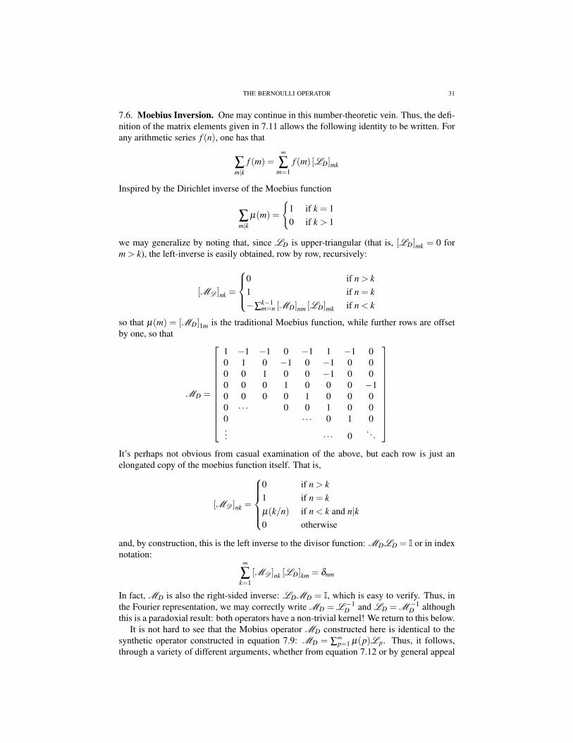
THE BERNOULLI OPERATOR 31
7.6. Moebius Inversion. One may continue in this number-theoretic vein. Thus, the defi-nition of the matrix elements given in 7.11 allows the following identity to be written. Forany arithmetic series f (n), one has that
∑m|k
f (m) =∞
∑m=1
f (m) [LD]mk
Inspired by the Dirichlet inverse of the Moebius function
∑m|k
µ(m) =
1 if k = 10 if k > 1
we may generalize by noting that, since LD is upper-triangular (that is, [LD]mk = 0 form > k), the left-inverse is easily obtained, row by row, recursively:
[MD ]nk =
0 if n > k1 if n = k−∑
k−1m=n [MD]nm [LD]mk if n < k
so that µ(m) = [MD]1m is the traditional Moebius function, while further rows are offsetby one, so that
MD =
1 −1 −1 0 −1 1 −1 00 1 0 −1 0 −1 0 00 0 1 0 0 −1 0 00 0 0 1 0 0 0 −10 0 0 0 1 0 0 00 · · · 0 0 1 0 00 · · · 0 1 0... · · · 0
. . .
It’s perhaps not obvious from casual examination of the above, but each row is just anelongated copy of the moebius function itself. That is,
[MD ]nk =
0 if n > k1 if n = kµ(k/n) if n < k and n|k0 otherwise
and, by construction, this is the left inverse to the divisor function: MDLD = I or in indexnotation:
∞
∑k=1
[MD ]nk [LD]km = δnm
In fact, MD is also the right-sided inverse: LDMD = I, which is easy to verify. Thus, inthe Fourier representation, we may correctly write MD = L −1
D and LD = M−1D although
this is a paradoxial result: both operators have a non-trivial kernel! We return to this below.It is not hard to see that the Mobius operator MD constructed here is identical to the
synthetic operator constructed in equation 7.9: MD = ∑∞p=1 µ(p)Lp. Thus, it follows,
through a variety of different arguments, whether from equation 7.12 or by general appeal

THE BERNOULLI OPERATOR 32
to operator theory, that the eigenvalues of MD are 1/ζ (s) and the eiegenvectors are v(s)with [v(s)]n = an = n−s are before:
MDv(s) =1
ζ (s)v(s)
The first row of the above operator equation is none other than the well-known Dirichletseries identity
∞
∑n=1
µ(n)ns =
1ζ (s)
and in fact, every row of the operator equation simply repeats this form. Going over to theFourier decomposition 7.1, the position-space eigenvectors are again given by equation 7.5(keeping in mind, as before, that we are ignoring the zero’th column/row, or, equivalently,that a0 = 0), and so one has that
[MDβ (s)] (x) =β (x;s)ζ (s)
with the same identity holding for β (1−x;s). Because the zeta function has only one pole,at s = 1, this implies that the Moebius operator has a two-dimensional kernel. It is spannedby the generator
β (x;1) =∞
∑n=1
e2πinx
πn
and by β (1− x;1). Unfortunately, these sums do a dis-service: really, the difference justgives the Bernoulli polynomial. That is, i
2 (β (x;1)−β (1− x;1)) = B1(x) = x− 12 , while
the sum 12 (β (x;1)+β (1− x;1)) = 1
πCl1(2πx) where Cl1(θ) is the Clausen function of
order 1. It is purely real, very smooth, having a U-shape, with singularities at x = 0 and 1.
7.6.1. Invertability and the Riemann Hypothesis. What is the correct way of understand-ing the operator equations MD = L −1
D and LD = M−1D given that both of these oper-
ators appear to have a non-trivial kernel? The resolution of the paradox requires pay-ing careful attention to the spaces on which they act. From the point of view of clas-sical number theory, the operators are restricted to act only on the Banach space l1 =(a1,a2,a3, · · ·) : ∑
∞n=1 |an|< ∞ of absolutely summable series. None of the singular so-
lutions belong to this space. Thus, the vector an = 1/n lies in the kernel of MD but it isclearly not l1-summable. That’s OK, because Fourier analysis asks for l2-summability, andthis vector is clearly summable with the l2 norm.
The situation for the divisor operator LD is a bit more confusing. Its kernel correspondsto the zeros of the Riemann zeta function. The vector an = n−s is again not summable in thel1-norm when ℜs≤ 1
2 , which is the region where all of the Riemann zeros are conjecturedto lie.
In that sense, we have a simple statement that is equivalent to the Riemann hypothesis.Assume that the Riemann zeta had a zero in the critical strip that did not lie on the criticalline. By symmetry, this zero is doubled. That is, write s = 1
2 +η + iτ for η ,τ real. If thereis a zero with η > 0, then there is a second zero at 1
2 −η + iτ . The zero with the positive
η corresponds to a series that is l2-summable. That is, we have that ∑∞n=1
∣∣∣n 12+η+iτ
∣∣∣2 < ∞
whenever η > 0. If the Riemann hypothesis holds, then we may conclude that the divisoroperator LD is not singular, and thus is invertible, on the space of Fourier series (i.e. seriesthat are l2-summable). We have already proven that LD is invertible on the Banach space

THE BERNOULLI OPERATOR 33
l1. If we could prove that it was invertible on the Banach space l2, then we would have aproof of the Riemann hypothesis.
Assuming RH, then we see that the operator LD is singular only when the space offunctions on which it acts can be properly analytically continued into the regions whereℜs≤ 1
2 .
7.7. More Number Theory. Further well-known identities from Dirichlet convolutionfollow in a similar fashion. Let 1 = (1,1,1, · · ·) be the row vector of all-ones; let ε =(1,0,0, · · ·) be the row vector with one in the first position, and then all zeros. Thenclearly, 1MD = ε is the operator equation analog of the Dirichlet convolution 1 ∗ µ = ε .The Moebius inversion formula, with states that g = f ∗ 1 if and only if f = g ∗ µ has aclear operator analog: G = FLD if and only if F = G MD which follows trivially fromthe identity LDMD = I which was obtained above. As before, this Dirichlet convolu-tion identity holds only on the space of l1-summable series, and it holds on the space ofl2-summable series, if RH holds. Clearly, the identities cannot hold when the space offunctions is expanded by analytic continuation, as the kernels of F and G would be, byconstruction, become tainted by the zeros of MD and LD.
By analogy, the generalized divisor operator corresponding to the sigma function is then
LΣ(z) =
1 1 1 1 1 1 · · ·0 2z 0 2z 0 2z 0 2z 0 · · ·0 0 3z 0 0 3z 0 0 3z 0 · · ·0 0 0 4z 0 0 0 4z 0 0 · · ·· · · 0 0 5z 0 0 0 5z 0 · · ·
6z . . .
where one has, as before, the sum-of-divisors function:
σz(n) = ∑m|n
mz =∞
∑k=1
[LΣ(z)]kn
Writing the diagonal operator [Z (z)]mk = mzδmk as
Z (z) =
1 0 0 0 00 2z 0 0 00 0 3z 0 0 · · ·0 0 0 4z 0 · · ·...
. . .
one obviously has, in this basis, that LΣ(z) = Z (z)LD. This is the operator analog of theDirichlet convolution σz = Idz ∗1. From the previous secion, we can deduce that Z (z) =LΣ(z)MD with is the operator analog of the convolution Idz = σz ∗µ .
The Euler totient function ϕ is given by the convolution ϕ = Id∗µ which suggests thatthe correct operator analog is P = Z (1)MD which has the following form:

THE BERNOULLI OPERATOR 34
P =
1 −1 −1 0 −1 1 −1 00 2 0 −2 0 −2 0 00 0 3 0 0 −3 0 00 0 0 4 0 0 0 −40 0 0 0 5 0 0 00 · · · 0 0 6 0 00 · · · 0 7 0... · · · 0
. . .
It is straight-forward to verify that the column sums give the Euler totient function: viz:
ϕ(n) =∞
∑k=1
[P]kn
Likewise, Jordan’s totient function, given by the convolution Jz = Idz ∗ µ has an operatoranalog that is given by J (z) = Z (z)MD. The Jordan totient function itself arises as thecolumn sums, as before:
Jz(n) =∞
∑k=1
[P(z)]kn
One may continue in a similar vein, and define the operator analogs for the Liouville func-tion, the von Mangoldt function, and so on. By means of the Fourier basis 7.1 and theBernoulli operator in this basis 7.2, each of these operator analogs are “synthetic” opera-tors that can be constructed from the (p-adic) Bernoulli operators.
There are multiple tasks which lie ahead:
• Explore the spectrum of the various operators defined above. As should be clearfrom the matrix form of LΣ(z) above, the diagonal values, and thus the spectrum,is well-behaved only when z < 0. Some form of analytic continuation is needed tomove to the region z > 0. Similar remarks apply for the totient function.
• Explore the analog to the Lambert series. This should be concistent with the otherdevelopments: its well-known that the Lambert series plays a role in the Eisensteinseries and in the Jacobi theta functions. It is also well-known that the modulargroup PSL(2,Z) describes the symmetries seen in these series. What is not well-known is the explicit relationship to the dyadic monoid and the Cantor set (each ofthese are effectively “half” of the modular group, so the traces of that relationshipshould survive.)
7.8. Multiplication theorem. The well-known multiplication theorem[35] of the specialfunctions follows from the general case for multiplicative functions, given below. A hintof the multiplication theorem is already visible in equation 3.3. Here, we give it full ex-pression.
Given some series fn, consider the synthetic operator
(7.13) F =∞
∑n=1
fnLn
Working in the Fourier representation, the operators Ln have the matrix elements
[Ln]mk = δmn,k

THE BERNOULLI OPERATOR 35
Acting on vector c = cn, the operator F gives
[F c]m =∞
∑k=1
∞
∑n=1
fnδmn,kck =∞
∑n=1
fncmn
If the series c = cn is totally multiplicative, then, by definition of multiplicativity, onehas that cmn = cmcn for all m,n, and so
[F c]m = cm
∞
∑n=1
fncn
Writing this as an operator equation, we have
F c = ( f · c)c
where the eigenvalue is the dot product f · c and c is the eigenvector. What have we donehere? For any series fn, we have constructed an operator F that has, as eigenvectors,any totally multiplicative series!
As one special case, we immeditately have that
Fβ (x;s) = λβ (x;s)
with the eigenvalue being the Dirichlet series λ = ∑∞n=1 fnn−s. But of course: the synthetic
operators 7.13 are just linear combinations, and so the eigenvectors are unchanged.
7.8.1. The Multiplication theorem. As another a special case, any totally multiplicativeseries is an eigenvector of the Bernoulli operator. That is:
Lpc = cpc
By analogy to the beta functions defined in7.5, the explicit functional form may be given:
γ(x) =∞
∑n=1
cn exp(2πinx)
Then γ(x) together with γ(1− x) satisfy the Ruelle-Frobenius-Perron operator or transferoperator of the Bernoulli map, as given in equation 3.3. That is, we have, by construction,that
(7.14) [Lpγ] (x) =1p
p−1
∑k=0
γ
(x+ k
p
)= cpγ(x)
This last is recognizable as the “multiplication theorem” of the special functions[35], thusgiving a general way of constructing functions that obey this theorem. By letting cn = n−s,and applying various limits, one obtains each of the well-known multiplication theoremsfor the special functions. The periodic zeta function, the Hurwitz zeta function, and theBernoulli polynomials were previously covered above. The polylogarithm follows easily,with little effort. The polygamma function presents a different and more interesting case.
For those multiplicative series that are not summable, some form of analytic continua-tion must be found, in order to give meaningful results.

THE BERNOULLI OPERATOR 36
7.8.2. Summability. The intersting question, from the point of view of having a functionalanalysis, is to answer the question “which totally multiplicative series belong to l1 or l2”?Of course, the series n−s for ℜs > 1 (or ℜs > 1
2 for l2) satisfy this requirement. Are thereother series? The usual suspects: the totient function, the divisor function, the Liouvillefunction, the von Mangoldt function are not actually totally multiplicative; they are multi-plicative only when thier arguments are coprime. The only well-known completely multi-plicative functions are the Liouville function, and the Dirichlet characters. The Liouvillefunction λ (n) is not l1-summable, but the function λ (n)n−s, for suitable s, is (the prod-uct of any two multiplicative functions is multiplicative). Likewise, the Dirichlet charatersχ(n) themselves are not summable, but the functions χ(n)n−s are.
There is another noteworthy possibility. If a(n) is a totally additive function, so thata(mn) = a(m)+ a(n), then cn = za(n) is totally mutiplicative, and is obviously summablefor |z|< 1. There are two well-known totally additive functions: Ω(n), the total number ofprime factors of n counted with multiplicity, and νp(n), the number of times that the primefactor p occurs in the factorization of n.
Since the product of any two multiplicative functions is multiplicative, we can createarbitrary chimeras, such as cn = za(n)n−s. Each of these gives a distinct set of eigenvectorequations. What is not clear is if, or how, any of these might be linear combinations of eachother. That is, fix a constant λ , so that Lpc = λc. What is the space spanned by all suchc’s? Can an orthogonal basis be given? What are the smallest sets of totally mutiplicativefunctions that span this space? None of these answers seem obvious. There is a veryrich collection of eigenfunctions of the Bernoulli operator, with no straightforward way ofcharacterizing them.
7.9. Hardy Classes. The p-adic Bernoulli operator is a (conjugate of a) shift operator.Given that equation 7.6 indicated that these all commute, one has a family of commutingshift operators. An operator that commutes with a shift operator may be called “analytic”,in a certain precise sense, and, given appropriate properties, can often be further factoredinto Hardy classes[25], in analogy to the factorization into inner and outer functions ofordinary Hardy space.
XXX Do this.
8. LATTICE MODEL TOPOLOGY
It is well-known that one-dimensional lattice models, and more generally, subshifts offinite type, can provide useful tools and insights for the study of one-dimensional iteratedmaps[23]. This section recaps the use of a one-dimensional spin lattice for the constructionof a class of Bernoulli operator eigenfunctions. In essence, the lattice models recapture theWold decomposition of section 7.2, but using a more articulated, richer vocabulary. Inparticular, the shift operator gets a more concrete interpretation as a translation on a lattice.
Consider a one-sided lattice of points, labeled by the positive integers, that is, by n ∈N.At each lattice location, a variable σn, called the “spin” (a name deriving from physics),can take one of p values, so that σn ∈ 0,1,2, · · · , p−1. The space of states of the latticeis then Ω = p× p×·· · = pω where we write p ≡ 0,1,2, · · · , p−1, letting the numberstand for the set. A given lattice configuration σ = (σ1,σ2, · · ·) ∈ Ω can be taken to beeither a p-adic number, or as a real number x, with the Cantor mapping x : Ω→ [0,1] fromthe set of all lattice configurations Ω to the unit interval [0,1] given by
(8.1) x(σ) =∞
∑n=1
σn p−n

THE BERNOULLI OPERATOR 37
This mapping allows every possible spin lattice configuration to be mapped into the unitinterval [0,1], although not vice-versa: the natural topology on the spin lattice is finer thanthe natural topology on the reals, in that, for example, σ = (0,1,1, · · ·) and (1,0,0, · · ·) areinequivalent lattice configurations, whereas the binary numbers 0.0111 . . . and 0.1000 . . .both represent the rational 1/2. Only certain rationals are double-pointed like this, whereasall irrationals correspond to a unique lattice configuration. For p = 2, the Stone represen-tation theorem applies.
Any Cartesian product of spaces has a natural topology, called the “product topol-ogy”; the basis of the topology are referred to as “cylinder sets”[18, 23]. Since the one-dimensional lattice is the Cartesian product of an infinite number of finite sets, the producttopology applies. In fact, the product topology will prove very nice to work with; it is a rea-sonably coarse topology, yet, it is compatible with the natural topology on the reals. Oneparticularly strong utility of the product topology is that it enables the definition and dis-cussion of measurable (integrable) functions that are discontinuous at all rational numbers;by contrast, such constructions are extremely awkward when using Fourier series, and, ofcourse, impossible in the language of analysis. We’ll construct many such functions here;in what follows, the product topology will be made great use of.
The product topology allows a set of fractal eigenfunctions to be constructed for theBernoulli operator. One begins by noting that the left-shift operator τ on the lattice, definedby
τ(σ) = τ((σ1,σ2, · · ·)) = (σ2,σ3, · · ·)corresponds exactly to the Bernoulli map:
x(τ(σ)) = 2x(σ)−b2x(σ)cwhere we’ve written x(σ) instead of x to help remind that x should be thought of as amap, not a real number. For the remainder of this section, this distinction will rarely bemade again, although every occurrence of x should be implicitly understood to be the mapx : Ω→ [0,1].
Consider now some arbitrary function V : Ω→ F , where F may be taken to be the fieldR, or C, or some arbitrary general field. Then, given some λ ∈ F , one may construct thesum
(8.2) H(σ) =∞
∑n=1
λnV (τn
σ)
where τnσ = (τ τ · · · τ)(σ) is simply the n-fold iteration of the shift operator. Inphysics, the function H is usually called the translation-invariant Hamiltonian for the sys-tem, while V is the interaction potential. For a one-sided lattice, H is not strictly translationinvariant, as
(8.3) H(τ(σ)) =∞
∑n=1
λnV (τn+1
σ) =H(σ)−V (σ)
λ
so that H is “almost” an eigenvector of τ , with eigenvalue 1/λ . Almost, because the one-sided lattice introduces a correction V/λ . For the bi-infinite, two-sided lattice, a trulytranslation-invariant Hamiltonian can be defined. The two-sided lattice model correspondsto the Bakers map, and is treated in greater detail in section 9.
If τ is the left-shift operator, then the analog of the transfer operator can be roughlytaken to be the right-shift operator. Since the lattice is one-sided, there exist p inequivalentright-shift operators Sk:
(8.4) Sk(σ1,σ2, · · ·) = (k,σ1,σ2, · · ·)

THE BERNOULLI OPERATOR 38
These right-shift operators are inverses to the left shift operator τ only on one side, in thatτ Sk is the identity, but Sk τ is not. Clearly, τ has no left-inverse, as τ throws away datain its action. For the p = 2 case, the shift operators act on the Cantor mapping as
x(S0(σ)) =x(σ)
2
x(S1(σ)) =1+ x(σ)
2
and so one may immediately recognize how to pose the Bernoulli operator on the latticemodel. For some arbitrary f : Ω→ F one defines
[LB f ] (σ) =12[ f (S0(σ))+ f (S1(σ))]
For the general p-adic case, this generalizes trivially:
Definition. The p-adic Bernoulli operator acting on the space of functionals of latticeconfigurations is given by
(8.5) [Lp f ] (σ) =1p
p−1
∑k=0
f (Sk(σ))
where Sk is the k’th right-shift operator.
The action of Lp on the Hamiltonian H is takes the form
(8.6) LpH = LpV +λH
This is easily shown by direct substitution.The critical result here is that H is an eigenvector provided that LpV = 0. Curiously,
this implies that functions in the kernel of LB can be used to construct eigenfunctionsof LB. The above construction is not limited the the Bernoulli operator, but clearly is ageneral result: it is essentially the Wold decomposition of section 7.2, but restated in a amore general form: rather than requiring a Hilbert space, it holds for arbitrary Cartesianproducts over arbitrary spaces, provided only that the summation in eqn 8.2 is convergent(and/or meets any other criteria for the space being worked).
One may construct a large number of general eigenfunctions, provided that on can findnon-trivial objects in the kernel, and provided that one is working in a topology where thesum of equation 8.2 converges.
8.1. Fractal eigenfunctions. The above derivation of the eigenfunctions assumed a latticemodel (Cartesian product) topology for the unit interval. Using equation 8.1 to regain thenatural topology on the real numbers, one may use the construction to rediscover the fullset of eigenfunctions of the Bernoulli operator. This is done explicitly in this section.
From equation 6.1, it was seen that the kernel of the Bernoulli operator consists of theodd harmonics of sine and cosine:
LB sin2π(2k+1)x = 0
LB cos2π(2k+1)x = 0
Here, k is a non-negative integer parametrizing the kernel; however, it will be more conve-nient to write exp2πi(2k+1)x and let k rang e over all integers, positive and negative. A

THE BERNOULLI OPERATOR 39
simple linear combination over positive and negative k will regain the real form. Insertingthese into equation 8.2, one has
H(x) =∞
∑n=0
λn exp(2π (2k+1)τ
nx)
which is an eigenfunction: LBH = λH. Because exp is periodic, we may replace τn(x) by2nx. Switching notation, one has a collection of eigenfunctions
(8.7) φBλ ,k(x) =
∞
∑n=0
λn exp(2πi 2n (2k+1)x)
for any k ∈ Z. This derivation allows λ ∈ F for any field F ; taking F to be the complexnumbers, the sum converges absolutely for the disk |λ |< 1 and conditionally for |λ |= 1,depending on whether λ is a root of unity or not.
The superscript B denotes that these are eigenfunctions for the p= 2 case of the Bernoullioperator. For the general case, one builds the eigenfunctions out of the shift states
v(p)n,k,r(x) = exp2πix(pk+ r) pn
for n ∈ N0, k ∈ Z and r the “remainder”, 0 < r < p.
Theorem 1. The functions v(p)n,k,r(x) are shift states of Lp, that is,
(8.8)[Lpv(p)
n,k,r
](x) = v(p)
n−1,k,r(x)
for n 6= 0 and[Lpv(p)
0,k,r
](x) = 0 for the n = 0 case.
Proof. This is obtained by simple substitution:[Lpv(p)
n,k,r
](x) =
1p
p−1
∑m=0
v(p)n,k,r
(x+m
p
)
=1p
exp[2πix(pk+ r) pn−1] p−1
∑m=0
exp[
2πimp(pk+ r)pn
]= v(p)
n−1,k,r(x)
The sum in the middle line above is a Gauss sum[1], and may be shown to equal p whenn 6= 0 and equal to zero otherwise.
The above relationship is reminiscent of of the creation and annihilation ladder operatorsof quantum mechanics. This correspondence can be made stronger, and is explored in alater section. The p-adic shift states of equation 8.8 can be trivially used to construct theeigenstates of the p-adic Bernoulli operator. These are given by
φ(p)λ ,k,r(x) =
∞
∑n=0
λn exp(2πix (pk+ r) pn)
which clearly obeyLpφ
(p)λ ,k,r = λφ
(p)λ ,k,r
These eigenfunctions are highly degenerate, and span an infinite-dimensional space la-beled by k and r. Any linear combination of these is also an eigenvector with the sameeigenvalue. These clearly form a continuous spectrum for the Bernoulli operator, although,strictly speaking, this spectrum is defined only on the unit disk |λ |< 1. This is in contrast to

THE BERNOULLI OPERATOR 40
FIGURE 8.1. Fractal Eigenfunction
-2
-1.5
-1
-0.5
0
0.5
1
1.5
2
0 0.1 0.2 0.3 0.4 0.5 0.6 0.7 0.8 0.9 1
phi(x)
x
Bernoulli eigenfunction, p=5, k=0, r=2
real partimaginary part
This figure shows the real and imaginary parts of the eigenfunction φ(p)λ ,k,r(x) = φ
(5)0.45,0,2(x).
The non-differentiability is clear visible. This function would be differentiable only forλ < 0.2; in that case, visually, the spikes would be completely smoothed away. The
twice-repeated sine-wave nature is entirely due to k = 2.
the zeta eigenfunctions, which are defined for the entire complex λ -plane (although theseare not integrable when |λ | > 1). This implies that the construction of eigenfunctions bymeans of lattice shifts is somehow innately limited: it allows some, but not all possibleeigenfunctions to be found. The true nature of this obstruction is unclear. The proximalcause of the obstruction is that ∑n λ n = 1/(1−λ ) has a pole at λ = 1, thus preventing theconvergence of the analytic series beyond that point. However, in the more global view,one has an operator acting on an infinite-dimensional topological vector space; whether theobstruction is due to the operator or the structure of the space itself is unclear.
8.2. Analytic properties. Unlike the zeta function eigenvectors, these eigenvectors arenot infinitely differentiable. Taking the first derivative, one has
ddx
φ(p)λ ,k,r(x) = 2πi(pk+ r)
∞
∑n=0
pnλ
n exp(2πix (pk+ r) pn)
and so the right hand side converges absolutely only if |λ | < 1/p. For |λ | > 1/p, theeigenfunction is continuous but not differentiable. This is visualized in figure 8.1. Secondderivatives may be taken only if |λ |< 1/p2; more generally, n’th derivatives may be takenonly when |λ |< 1/pn.
Clearly, any linear combination of only a finite number of these fractal eigenfunctionswill posses similar analytic properties. However, there is an infinite series combination

THE BERNOULLI OPERATOR 41
of these that does reproduce the zeta function eigenfunctions. An explicit relationshipbetween these two is developed in the next section.
8.3. The Fractal Spectrum. The fractal spectrum can be re-expressed in terms of the zetaeigenfunctions, and vice-versa. That is, the one set of eigenfunctions can be expressed aslinear combinations of the other. This section gives the explicit linear relations connectingthe one to the other.
The establishment of this result is the observation that every integer has a unique factor-ization in the form of (pk+r)pn, with k,r and n uniquely determined when p is fixed. Thisleads to a summation identity: for a fixed integer p, and some arbitrary summable functionf (n), one has
∞
∑n=0
f (n) =∞
∑k=0
p−1
∑r=1
∞
∑m=0
f ((pk+ r)pm)
The summand of the triple sum on the right is precisely of the form appearing in the fractaleigenfunctions, whereas the left-hand side is of the simpler form of the zeta eigenfunctions.The desired linear relationship is obtained merely by matching terms in the series. That is,one sets f (n) = 2Γ(s+1)(2πn)−s exp(2πixn) to immediately obtain
β (x;s) =2Γ(s+1)(2π)s
∞
∑k=0
p−1
∑r=1
1(pk+ r)s
∞
∑m=0
exp2πix(pk+ r)pm
pms
=2Γ(s+1)(2π)s
∞
∑k=0
p−1
∑r=1
1(pk+ r)s φ
(p)λ ,k,r(x)
where one identifies λ = p−s.The full set of zeta eigenfunctions, accounting for degeneracy, is given by
βn(x;s)≡ β (x;s+2πni/ ln2)
with n ∈ Z. These share the same eigenvalue: Lpβn = p−sβn. The relevant values ofs should be restricted to a principal domain −π < ℑs ln2 = arg z < π . Repeating theabove manipulations, the goal is to write the zetas as a linear combination of the fractaleigenfunctions, so:
βn(x;s) =∞
∑k=0
p−1
∑r=1
Fnkr φ(p)λ ,k,r(x)
These matrix elements are
Fnkr = 2Γ
(s+1+
2πniln2
)(2π(pk+ r))−s exp
[−2nπi
lnπ(pk+ r)ln2
]Presumably F is invertible; the φ
(p)λ ,k,r should be expressible in terms of the βn(x;s).
The analytic situation is curious: the zeta eigenfunctions are well-defined for |λ | > 1,even as the fractal eigenfunctions are not. The change-of-basis summations clearly appearto be divergent as |λ | approaches 1. It would appear that the zeta eigenfunctions span alarger space than the fractal eigenfunctions.
8.4. Discontinuous eigenfunctions. Some of the eigenfunctions are not continuous inthe natural topology of the reals. Thus, for example, given the expansion in binary digitsbn ∈ 0,1 of a real number 0≤ x≤ 1,
x =∞
∑n=0
bn
2n+1

THE BERNOULLI OPERATOR 42
FIGURE 8.2. Devil’s staircase
-1
-0.8
-0.6
-0.4
-0.2
0
0.2
0.4
0.6
0.8
1
0 0.2 0.4 0.6 0.8 1
c(x
)
x
Devil’s Staircase
This figure shows a graph of the eigenfunction cλ (x) for λ = 0.4. As can be clearly seen,it takes on values in the Cantor set.
Then the Cantor or “Devil’s staircase” function
cλ (x) = λ (λ −1)∞
∑n=0
(−1)bn λn
is easily shown to be an eigenfunction of LB with eigenvalue λ . This function is clearlydiscontinuous for all λ except λ = 1/2, where cλ (x) = B1 (x) = x− 1/2. The Devil’sstaircase function is shown in 8.4.
This eigenfunction is not ’new’, but is rather a linear combination of those alreadypresented. To see this, generalize the construction. The φ
(p)λ ,k,r(x) were built up explicitly
from sine waves, but there is no particular reason to start with a sine-wave basis for thekernel. Consider, for example, the square wave or Haar wavelet
h(x) =
+1 for 0≤ x < 1/2−1 for 1/2≤ x < 1
extended to the entire real-number line as a periodic function h(x+n) = h(x) for integer n.The Haar wavelet is in the kernel of the Bernoulli operator: LBh(x) = 0, and thus can beused to create a fractal eigenfunction by means of the lattice shift equation 8.6:
(8.9) ψk(x) =∞
∑n=0
λnh((2k+1)2nx)

THE BERNOULLI OPERATOR 43
so that LBψk = λψk for any |λ | < 1 in the unit disk. Of course, cλ is a special case:cλ (x) = λ (λ −1)ψ0 (x), and so we see that cλ is a linear combination of the functions 8.7.By the Fourier decomposition theorem, any periodic function odd about 1/2 will consistentirely of odd harmonics, and can thus be used to define an eigenfunction in the mannerof eqn8.9. That it is a linear combination of the basis vectors 8.7 follows trivially.
There are a few practical reasons for choosing a basis other than the sine-wave ba-sis. Most notably, convergence properties are altered: the Haar wavelet can avoid theGibbs phenomenon of “ringing” that makes absolute bounds difficult to establish. TheHaar wavelet also seems more compatible with the product topology of the lattice; it has aparticularly simple form when considered as a function on the lattice.
Note, incidentally, that even more ’horrible’ eigenfunctions can be constructed in thisfashion. Consider, for example, δ
(x− 1
4
)−δ
(x− 3
4
), extended to be periodic on the real
line. It may be expressed as a Fourier series; it lies in the kernel of LB. It may be usedto create a fractal eigenfunction: integrable but not square-integrable and certainly notbounded, thus showing that there are eigenfunctions of LB that are in L1 but not in L2or L∞. This foreshadows some of the more challenging functions one encounters whenanalyzing other transfer operators, such as the GKW operator[28]. It also vindicates thefocus on measurable functions on the product topology: the Dirac delta function is fareasier to ’understand’ as a measure on a topology than as a Fourier series.
8.5. Fractal Symmetry and the Dyadic Monoid. ————xxxxxxxxxxxx————xxxxxxxxThe fractal eigenfunctions are self-similar. This self-similarity follows directly from the
shift invariance of the lattice construction, that is, of the translation invariance of the latticeHamiltonian embodied in equation 8.3. Loosely speaking, one might say that translation-invariant Hamiltonians must necessarily have fractal eigenfunctions. The self-similaritieshave a non-trivial structure, which is exposed in this section.
For concreteness, consider first the action of the right-sift operators S0 and S1, definedby equation 8.4, acting on the k = 0 dyadic eigenfunction 8.9 built from the Haar wavelet.One has (dropping the subscript k fromψ):
[S0 ·ψ] (x) = ψ
( x2
)=
∞
∑n=0
λnh(2n−1x
)= h
( x2
)+λ
∞
∑n=1
λn−1h
(2n−1x
)= h
( x2
)+λψ(x)
= −1+λψ(x)
with the last step following because the Haar wavelet is identically -1 on the interval 0 ≤x < 1/2. To emphasize this, write it more simply as
ψ
( x2
)=−1+λψ(x)
That is, one very explicitly has that the eigenfunction on the whole unit interval looksexactly like the eigenfunction on the half-interval, except that its scaled and offset: this isclassic fractal self-similarity.

THE BERNOULLI OPERATOR 44
For the other shift operator S1, one readily obtains that S1ψ = 1+ λψ . The actionof these two shift operators has a representation in terms of 2x2 matrices acting on two-dimensional vectors. The basis vectors e0 and e1 for this vector space are
1 7→ e0 =
[10
]and ψ 7→ e1 =
[01
]one has
(8.10) S0 =
[1 −10 λ
]and S1 =
[1 10 λ
]so that one has, for example S0e1 =−e0 +λe1 as the action of the right shift on this vectorspace. The two matrices S0 and S1 generate a monoid, the dyadic monoid. A generalelement γ of the monoid is then
γ = Sn00 Sn1
1 Sn20 Sn3
1 · · ·
for non-negative integers n0,n1,n2, · · · . The monoid is free, in that there are no relationsbetween S0 and S1, and each unique string of integers n0,n1,n2, · · · results in a uniqueelement of the monoid. For the purpose of this text, a monoid is defined much as a group,except that inverses are not considered. This is for two reasons: first, the inverses of S0and S1 are not uniquely defined: the left and right inverse differ. Secondly, γ is to beunderstood to be the action of a monoid element acting on the unit interval. As long asthe action maps the whole interval into a sub-interval, the action is well-defined; however,there are technical difficulties with going in the reverse direction.
The dyadic monoid has many interesting properties; these are discussed in greater detailin [30]. Among the notable properties is that the dyadic monoid is isomorphic to a certainsubset of the Modular Group; this connection alone being important as the modular groupplays an important role in number theory, specifically in the area of modular forms andautomorphic forms. Not inconsequential is that the theory of modular forms again borderson the theory of the Riemann zeta. In a similar vein, one notes that the string of integers[n0,n1,n2, · · · ] is isomorphic to a continued fraction. Continued fractions are importantboth to the theory of Diophantine equations (Pellian equations), and in turn are seen to tieback into general phenomena seen in ergodic dynamics.
The integral of the Haar wavelet or square wave is the tent map or triangle wave
t(x) =∫ x
0h(y)dy =
12 −2x when 0≤ x≤ 1/2− 3
2 +2x when 1/2≤ x≤ 1
This is extended to the entire real line by defining t(x+n) = t(x) for integer n. The trianglewave has the curious property of period-doubling upon iteration: that is, tk(x) =−t(2k−1x)for k > 1. The iterated tent map behaves as a shift state, in that the Bernoulli operator actsas an annihilation operator: [
LBtk](x) = tk−1(x)
with the shift terminating at k = 1:
[LBt] (x) = 0
The fractal eigenfunction constructed from the triangle wave is the Takagi or blancmangecurve:
bλ (x) =∞
∑n=0
λnt(2nx)

THE BERNOULLI OPERATOR 45
and so of course, LBbλ = λbλ . There is a curious special case: the Takagi curve b1/4(x) isa parabola, corresponding to the Bernoulli polynomial B2(x). Apparently, the constructionof the parabola by self-similar subdivision was known to Archimedes[22].
The blancmange curve transforms under a three-dimensional representation as the Haar-wavelet curve, in that
S0bλ =−(
x− 12
)+λbλ and S1bλ =
(x− 1
2
)+λbλ
Taking as the basis vectors
1 7→ e0 =
100
x 7→ e1 =
010
bλ 7→ e2 =
001
the two generators may be written as
S0 =
1 0 12
0 12 − 1
20 0 λ
and S1 =
1 12 − 1
20 1
212
0 0 λ
This process can be extended arbitrarily. One may choose to integrate the triangle wave,
or to make a more general ansatz. Given some arbitrary polynomial p(x), one may fashiona piece-wise polynomial periodic wave
q(x) =−p(x) when 0≤ x < 1/2
p(x− 1
2
)when 1/2≤ x < 1
so that q(x+ 1/2) = −q(x) or equivalently, [LBq] (x) = 0. From this, one constructs thefractal wave
fλ (x) =∞
∑n=0
λnq(2nx)
which transforms as
S0 fλ =−p( x
2
)+λ fλ and S1 fλ = p
( x2
)+λ fλ
If the degree of the polynomial is m, then the associated linear representation is m+ 2dimensional. One may choose as the basis vectors ek = xk for k ≤ m and em+1 = fλ . Thematrix forms of S0 and S1 are obtained by expanding the polynomial p(x/2) in terms ofthe chosen basis. There is nothing special about the monomial basis; one might considerany basis where ek represents a polynomial of degree k.
As should be clear from the above construction, when q(x) is not a polynomial, the rep-resentation cannot be finite-dimensional. In particular, the sine-wave based dyadic fractal8.7 constructed from q(x) = exp2πix does not transform under a finite-dimensional repre-sentation.
The general dyadic case k 6= 0, given by
fλ ,k(x) =∞
∑n=0
λnq(2n (2k+1)x)

THE BERNOULLI OPERATOR 46
does not change the situation. Since [LBq] (x) = 0, one has q(x+ 1/2) = −q(x), and soagain, the action of S0 and S1 is given by
S0 fλ ,k = q((2k+1)
x2
)+λ fλ ,k and S1 fλ ,k =−q
((2k+1)
x2
)+λ fλ ,k
As before, if q(x) is made from a polynomial of degree m, the resulting fractal functiontransforms under an m+2 dimensional linear representation.
The general p-adic case proceeds in a similar manner. Polynomials of degree m trans-form as an m + 2 dimensional representation, just as before. There are no longer twogenerators, but p generators S0,S1, · · · ,Sp−1.
XXXX Would deeper properties of the dyadic monoid be worth reviewing here???XXXX – When are the inf-dimensional reps conjugate? What are conjugacy classes?
etc.XXXX more info on the p-adic free monoids, please.
8.6. Number theoretic connections. For prime number p, the number theoretic Heckeoperator[2] may be written as
[Tp f ] (τ) = pm−1 f (pτ)+1p
p−1
∑k=0
f(
τ + kp
)In number theory, the Hecke operator is used in the classification of modular forms of orderm. Now, in number theory, the above is intended to act only on functions meromorphic inthe upper-half complex plane; i.e. for which τ lies in the upper half of the complex plane.However, we can immediately recognize the Hecke operator as the sum of the Bernoullioperator and its transpose:
Tp = pm−1Kp +Lp
and so a certain form of the Hecke operator may be defined as acting on the unit intervaland/or the Cantor set with the product topology. XXX expand, clarify.
Another curious operator is the Gauss-sum-like extension[L
(m)p f
](σ) =
1p
p−1
∑k=0
e2πikm/p f (Sk(σ))
regaining Lp = L(0)p .
9. TWO-SIDED LATTICE
The two-sided lattice is the lattice that stretches off to both the left and the right. Thestate of the two-sided lattice may be represented by two numbers 0≤ x,y≤ 1 with x givenby equation ??, and y likewise, but instead being a sum over the negative indexes, startingat k = −1. The energy is a simple sum of the energy of the half-lattices to the left and tothe right, plus an interaction term involving spins on both the left and right. The proba-bility density is a product of the probability densities on the left and right, adjusted by theinteraction between the left and right sides.
The shift operator τ can be understood to be an operator that pops a bit off the right-hand half lattice, and pushes it onto the left half-lattice. In the dyadic notation, it can berecognized as the so-called Baker’s map, a map from the unit square onto itself that cutsthe square into two pieces, and stacks and squashes them. That is, given a pair of numbers(x,y) in the unit square, one has
τ(x,y) =(
x+ b2yc2
, 2y−b2yc)

THE BERNOULLI OPERATOR 47
FIGURE 9.1. Ising Tartan
This tartan-like graph shows the Ising model probability density P(σ) for the two-sidedlattice using the dyadic mapping. That is, the lattice configuration
σ = (σ−N−1, · · · ,σ−2,σ−1,σ0,σ1,σ2, · · · ,σN) is represented by two numbers 0≤ x,y≤ 1with
x(σ) =N
∑k=0
(σk +1
2
)2−(k+1)
and
y(σ) =N
∑k=0
(σ−k−1 +1
2
)2−(k+1)
The energy of a given configuration σ is computed using ??, with the sum running from−N to +N, of course. The probability density P(σ) is given by equation ??.
The graph here assumes the Ising potential, with J = 0.3 and M = 0 for a finite sizedlattice with N = 10. The color choices here are such that black represents values whereP(σ) = P(x,y) are zero, blue are small values, with yellow and red being progressively
larger values. This fractal tartan is invariant under the Baker’s map.

THE BERNOULLI OPERATOR 48
The Baker’s map can be studied in its own right as a discrete-time dynamical system, inthat τ can be taken to define the time evolution of a unit square over a single time-step.The time evolution is invertible, in that the inverse map τ−1 is uniquely defined, being
τ−1(x,y) =
(2x−b2xc , y+ b2xc
2
)The inverse map can be seen to be identical to the forward map with x and y interchanged:that is, translation to the left on the lattice is identical to translation to the right, with leftand right exchanged. One may say the map is PT -symmetric, with P standing for the“parity exchange” operation x↔ y and T being the “time inversion” operator τ ↔ τ−1.
The two-sided lattice may be studied either as a lattice model, or as a dynamical systemwith time evolution given by τ . It is interesting to juxtapose these two viewpoints. Asa lattice model, one is typically only interested in lattices for which the energy and theprobability density are invariant under the action of the translation operator. That is, one isinterested only in the classical Hamiltonians of eqn ?? which are translation-invariant:
H (τnσ) = H (σ)
for all n ∈ Z.Considered as a dynamical system, one is typically interested in the time evolution of
densities on the unit square, that is, of real-valued maps ρ : [0,1]× [0,1]→ R. The timeevolution of a density can be simply understood as a physical model, where the density isa local density of some “dust” of points (x,y), with the time evolution of each point givenby τ . Thus, the time evolution of this “dust” or density is given by the transfer operatorLT as
[LT ρ] (x,y) =(ρ τ
−1)(x,y) = ρ
(2x−b2xc , y+ b2xc
2
)The transfer operator is thus a map LT : F → F where F is the set of functions onthe unit square. Clearly LT is a linear operator. Here, the subscript T on LT is used toremind us that this is now the transfer operator on the two-sided lattice; it can be writtenas a combination of LB and the Koopman operator KB for the single-sided lattice. One isinterested in characterizing the eigenfunctions and eigenvalues of LT .
The general idea behind equation ?? can be immediately appealed to, to construct someof the eigenstates of LT . That is, on considers functions f (x,y) of the form
(9.1) f =∞
∑n=−∞
λng τ
n
given some function g(x,y) and number λ . Formally, such an f is an eigenstate of LT witheigenvalue λ : that is, LT f = λ f . In practical terms, it is evident that not all possible λ canmake the sum convergent, although one might expect that λ on the unit circle |λ |= 1 of thecomplex plane might lead to a convergent sum. Thus immediately, one deduces that LTmust surely be a unitary operator. The unitarity of LT makes intuitive sense in a certainway: the map τ is invertible, and one expects time-reversible evolution to be described byunitary operators. The figure 9.1 shows a tartan-like distribution corresponding to λ = 1and g(x,y) =VIsing(x) the Ising model potential. Some additional tartans, for other valuesof λ , are shown in figure xx.
The proper analysis of the transfer operator LT requires that the function space Fbe pinned down more precisely. Classic results on time-symmetry breaking [16, 13, 6]indicate that whether or not LT is unitary depends on the function space F .

THE BERNOULLI OPERATOR 49
9.1. Ladder operators. Simple Harmonic Oscillator review.There are several related, intertwined confusions, here. There lattice allows two differ-
ent interpretations of what it means to be a ladder operator. XXX finish me.
10. MEASURE-THEORETIC DESCRIPTION
In this section, it will be shown that the transfer operator is the push-forward of the shiftoperator; a theorem and a sequence of lemmas will be posed, that hold in general form.The point of this theorem is to disentangle the role of topology, and specifically, the role ofmeasure theory, from the use of the shift operator. We begin with a general setting.
Consider a topological space X , and a field F over the reals R. Here, F may be taken tobe R itself, or C or some more general field over R. The restriction of F to being a fieldover the reals is is required, so that it can be used in conjunction with a measure; measuresare always real-valued.
One may then define the algebra of functions F (X) on X as the set of functionsf ∈ F (X) such that f : X → F . An algebra is a vector space endowed with multipli-cation between vectors. The space F (X) is a vector space, in that given two functionsf1, f2 ∈ F (X), their linear combination a f1 + b f2 is also an element of F (X); thus f1and f2 may be interpreted to be the vectors of a vector space. Multiplication is the point-wise multiplication of function values; that is, the product f1 f2 is defined as the function( f1 f2)(x) = f1(x) · f2(x), and so f1 f2 is again an element of F (X). Since one clearly hasf1 f2 = f2 f1, multiplication is commutative, and so F (X) is also a commutative ring.
The space F (X) may be endowed with a topology. The coarsest topology on F (X) isthe weak topology, which is obtained by taking F (X) to be the space that is topologicaldual to X . As a vector space, F (X) may be endowed with a norm ‖ f‖. For example, onemay take the norm to be the Lp-norm
‖ f‖p =
(∫| f (x)|p dx
)1/p
For p = 2, this norm converts the space F (X) into the Hilbert space of square-integrablefunctions on X . Other norms are possible, in which case F (X) has the structure of aBanach space rather than a Hilbert space.
Consider now a homomorphism of topological spaces g : X → Y . This homomorphisminduces the pullback g∗ : F (Y )→ F (X) on the algebra of functions, by mapping f 7→g∗( f ) = f g so that f g : Y → F . The pullback is a linear operator, in that
g∗(a f1 +b f2) = ag∗( f1)+bg∗( f2)
That the pullback is linear is easily demonstrated by considering how g∗ f acts at a point:(g∗ f )(x) = ( f g)(x) = f (g(x)) and so the linearity of g∗ on a f1 +b f2 follows trivially.
One may construct an analogous mapping, but going in the opposite direction, calledthe push-forward: g∗ : F (X)→F (Y ). There are two ways of defining a push-forward.One way is to define it in terms of the sheaves of functions on subsets of X and Y . Thesheaf-theoretic description is more or less insensitive to the ideas of measurability, whereasthis is important to the definition of the transfer operator, as witnessed by the appearance ofthe Jacobian determinant in equation 2.2. By contrast, the measure-theoretic push-forwardcaptures this desirable aspect. It may be defined as follows.
One endows the spaces X and Y with sigma-algebras (X ,A ) and (Y,B), so that Ais the set of subsets of X obeying the axioms of a sigma-algebra, and similarly for B.A mapping g : X → Y is called “measurable” if, for all Borel sets B ∈ B, one has thepre-image g−1(B) ∈A being a Borel set as well. Thus, a measurable mapping induces a

THE BERNOULLI OPERATOR 50
push-forward on the sigma-algebras: that is, one has a push-forward g∗ : F (A )→F (B)given by f 7→ g∗( f ) = f g−1, which is defined by virtue of the measurability of g. Thepush-forward is a linear operator, in that
g∗(a f1 +b f2) = ag∗( f1)+bg∗( f2)
One regains the transfer operator as defined in equation 2.2 by considering the limitingbehavior of the push-forward on progressively smaller sets. That is, one has
Theorem 2. The transfer operator is the point-set topology limit of the measure-theoreticpush-forward.
Proof. The proof that follows is informal, so as to keep it simple. It is aimed mostly atarticulating the language and terminology of measure theory. The result is none-the-lessrigorous, if taken within the confines of the definitions presented.
Introduce a measure µ : A → R+ and analogously ν : B → R+. The mapping g ismeasure-preserving if ν is a push-forward of µ , that is, if ν = g∗µ = µ g−1. The measureis used to rigorously define integration on X and Y . Elements of F (A ) can be informallyunderstood to be integrals, in that f (A) for A ∈A may be understood as
f (A) =∫
Af (z)dµ(z) =
∫A
f (z)∣∣µ ′(z)∣∣dz
where |µ ′(x)| is to be understood as the Jacobean determinant at a point x ∈ X . Here, fcan be understood to be a function that is being integrated over the set A, whose integral isdenoted by f (A). The value of f at a point x ∈ X can be obtained by means of a limit. Oneconsiders a sequence of A ∈ A , each successively smaller than the last, each containingthe point x. One then has
lim−−→A3x
f (A)µ(A)
= f (x)
which can be intuitively proved by considering A so small that f is approximately constantover A:
f (A) =∫
Af (z)dµ(z)≈ f (x)
∫A
dµ = f (x)µ(A)
To perform the analogous limit for the push-forward, one must consider a point y ∈ Yand sets B ∈ B containing y. In what follows, it is now assumed that g : X → Y is amulti-sheeted countable covering of Y by X . By this it is meant that for any y that is nota branch-point, there is a nice neighborhood of y such that its pre-image consists of theunion of an at most countable number of pair-wise disjoint sets. That is, for y not a branchpoint, and for B 3 y sufficiently small, one may write
g−1(B) = A1∪A2∪·· ·=k⋃
j=1
A j
where k is either finite or stands for ∞, and where Ai∩A j =∅ for all i 6= j. At branch points,such a decomposition may not be possible. The axiom of sigma-additivity guarantees thatsuch multi-sheeted covers behave just the way one expects integrals to behave: in otherwords, one has
µ(g−1(B)
)= µ
(k⋃
j=1
A j
)=
k
∑j=1
µ (A j)

THE BERNOULLI OPERATOR 51
whenever the collection of A j are pair-wise disjoint. Similarly, in order to have the elementsf ∈F (A ) behave as one expects integrals to behave, one must restrict F (A ) to containonly sigma-additive functions as well, so that
f(g−1(B)
)= f
(k⋃
j=1
A j
)=
k
∑j=1
f (A j)
As the set B is taken to be smaller and smaller, the sets A j will become smaller as well.Denote by x j the corresponding limit point of each A j, so that g(x j) = y and the pre-imageof y consists of these points: g−1(y) =
x1,x2, · · ·
∣∣g(x j) = y
. One now combines theseprovisions to write [
g∗ f](y) = lim−−→
B3y
[(g∗ f )(B)
ν(B)
]
= lim−−→B3y
[(f g−1
)(B)
ν(B)
]
= lim−−−−−−−→A j3g−1(y)
f (A1∪A2∪·· ·)ν(B)
= lim−−−−−−−→A j3g−1(y)
∑kj=1 f (A j)
ν(B)
=k
∑j=1
f (x j) lim−−−→A j3x j
µ (A j)
ν(B)(10.1)
The limit in the last line of this sequence of manipulations may be interpreted in two ways,depending on whether one wants to define the measure ν on Y to be the push-forward ofµ , or not. If one does take it to be the push-forward, so that ν = g∗µ , then one has
lim−−−→A j3x j
µ (A j)
g∗µ(B)=
1∣∣g′ (x j)∣∣
where∣∣g′ (x j)
∣∣ is the Jacobian determinant of g at x j. This last is a standard result ofmeasure theory, and can be intuitively proved by noting that g(A j) = B, so that
ν (B) =∫
A j
g′(z)dµ(z)≈ g′ (x j)µ (A j)
for “small enough” B. Assembling this with the previous result, one has
(10.2)[g∗ f](y) = ∑
x j∈g−1(y)
f (x j)∣∣g′ (x j)∣∣
which may be easily recognized as equation 2.2. This concludes the proof of the theorem,that the transfer operator is just the point-set topology limit of the push-forward.
In simplistic terms, the push-forward can be thought of as a kind of change-of-variable.Thus, one should not be surprised by the following lemma, which should be recognizableas the Jacobian, from basic calculus.
Lemma 3. (Jacobian) One has
∑x j∈g−1(y)
1∣∣g′ (x j)∣∣ = 1

THE BERNOULLI OPERATOR 52
Proof. This follows by taking the limit−−−−→A j 3 x j of
µ (A j)
g∗µ(B)=
µ (A j)
∑ki=1 µ (Ai)
and then summing over j.
Corollary 4. The uniform distribution (i.e. the measure) is an eigenvector of the transferoperator, associated with the eigenvalue one.
Proof. This may be proved in two ways. From the viewpoint of point-sets, one simplytakes f = const. in equation 10.2, and applies the lemma above. From the viewpoint of thesigma-algebra, this is nothing more than a rephrasing of the starting point, that ν = g∗µ ,and then taking the space Y = X , so that the push-forward induced by g : X → X is ameasure-preserving map: g∗µ = µ .
The last corollary is more enlightening when it is turned on its side; it implies twowell-known theorems, which follow easily in this framework.
Corollary 5. (Ruelle-Perron-Frobenius theorem). All transfer operators are continuous,compact, bounded operators; furthermore, they are isometries of Banach spaces.
Proof. This theorem is of course just the Frobenius-Perron theorem, recast in the contextof measure theory. By definition, the measures have unit norm: that is, ‖µ‖1 = 1 and‖ν‖1 = 1. This is nothing more than the statement that the spaces X and Y are measurable:the total volume of X and Y is, by definition, one. Since ν = g∗µ , we have ‖g∗µ‖1 = 1,and this holds for all possible measures µ ∈F (X).
Recall the definition of a bounded operator. Given a linear map T : U → V betweenBanach spaces Uand V , then T is bounded if there exists a constant C < ∞ such that‖Tu‖V ≤ C‖u‖U for all u ∈U . But this is exactly the case above, with T = g∗, and U =F (X), V = F (Y ), and C = 1. The norm of a bounded operator is conventionally definedas
‖T‖= supu 6=0
‖Tu‖V‖u‖U
= sup‖u‖U≤1
‖Tu‖V
and so we have the norm of g∗ being ‖g∗‖ = 1. That g∗ is an isometry follows triviallyfrom ‖g∗µ‖1 = ‖ν‖1 and that g∗ is linear.
The corollary 4 can also be treated as a corollary to the Perron-Frobenius theorem:namely, that there is at least one vector that corresponds to the maximum eigenvalue of g∗.This eigenvector is in fact the Haar measure, as the next theorem shows.
Theorem 6. (Haar measure) For any homomorphism g : X → X, one may find a measureµ such that g∗µ = µ; that is, every homomorphism g of X induces a measure µ on X suchthat g is a measure-preserving map. If g is ergodic, then the measure is unique.
Proof. By definition, µ is a fixed point of g∗. The fixed point exists because g∗is a boundedoperator, and the space of measures is compact, and so a bounded operator on a compactspace will have a fixed point. The existence of the fixed point is given by the Markov-Kakutani theorem[7, p 456]. The Markov-Kakutani theorem also provides the uniquenesscondition: if there are other push-forwards h∗ that commute with g∗, then each such push-forward will also have a fixed point. The goal is then to show that when g is ergodic,there are no other functions h that commute with g. But this follows from the definitionof ergodicity: when g is ergodic, there are no invariant subspaces, and the orbit of g is

THE BERNOULLI OPERATOR 53
the whole space. As there are no invariant subspaces, there are no operators that can mapbetween these subspaces, i.e. there are no other commuting operators.
A peculiar special case is worth mentioning: if g is not ergodic on the whole space,then typically one has that the orbit of g splits or foliates the measure space into a bunch ofpairwise disjoint leaves, with g being ergodic on each leaf. The Markov-Kakutani theoremthen implies that there is a distinct fixed point µ in each leaf, and that there is a mappingthat takes µ in one leaf to that in another.
In the language of dynamical systems, the push-forward g∗ is commonly written as Lg,so that one has
g∗ = Lg : F (X)→F (X)
now being called the transfer operator or the Ruelle-Frobenius-Perron operator.In the language of physics, the fixed point µ is called the “ground state” of a system.
When it is unique, then the ground state is not degenerate; when it is not unique, then theground state is said to be degenerate. The operator g∗ is the time-evolution operator of thesystem; it shows how physical fields f ∈F (X) over a space X evolve over time. When Fis the complex numbers C, the fact that ‖g∗‖= 1 is essentially a way of stating that time-evolution is unitary; the Frobenius-Perron operator is the unitary time-evolution operatorof the system. What is called “second quantization” in physics should be interpreted as thefitting of the space F (X) with a set of basis vectors, together with a formulation of g∗ interms of that basis.
XXX ToDo: This means the Koopman operator is the pullback. Since pullback andpush-forward are category-theoretic adjoints, nail down more of the category theory bits &pieces. Make it tight. Probably split this off into its own paper ...
11. THE TOPOLOGICAL ZETA
XXX ToDo: explain topo zeta gets this has this name, and why this concept is important.XXX
The topological zeta of the Bernoulli operator can be computed very easily in the poly-nomial basis because we know the eigenvalues and these form a simple series. We’ll definethe Bernoulli topological zeta as
ζB(t)≡1
det [I− tLB]
We start by noting its inverse:
det [I− tLB] =∞
∏n=0
(1− t 2−n)
= 1− t∞
∑j=0
2− j + t2∞
∑j=0
2− j∞
∑k = 0k 6= j
2−k− t3...
= 1−2t +83
t2− 167
t3 +128105
t4− ...(11.1)

THE BERNOULLI OPERATOR 54
Successive terms of this series are hard to compute, and it would be interesting to knowwhat the generating function for this series is. The series appears to have a circle of con-vergence of radius one. The zeta can be computed directly by working with its logarithm:
logζB(t) = log∞
∏n=0
(1− t 2−n)−1
= −∞
∑n=0
log(1− t 2−n)
=∞
∑k=1
tk
k2k
2k−1
= − log(1− t)+∞
∑k=1
tk
k1
2k−1(11.2)
Thus we have TrL kB = 2k/(2k − 1). Of some curiosity is the proximity of the Erdos-
Borwein constant:
1.6066... =∞
∑n=1
12n−1
=∞
∑n=1
d(n)2n(11.3)
which marks the first appearance of a classical number-theoretic function in the proceed-ings so far: d(n) is the number of divisors of n. This arises from the Lambert series
∞
∑n=1
d(n)xn =∞
∑n=1
xn
1− xn
The sum
E(t) =∞
∑k=1
tk
1−2−k
can be re-summed as a Lambert series, namely,
E(t) =∞
∑k=1
bk2−k
where
bk = ∑n|k(2t)n
The analytic/meromorphic structure of this zeta is not clear; its dull within the unit disk,and its not quite obvious what the continuation is outside of the disk. XXX ToDo: get thefull analytic structure.
12. CURIOSITIES
We list here some intriguing forms that suggest further relationships.The Pochhammer symbol (a)n = Γ(a+ n)/Γ(n) obeys a dimidiation formula that is
reminiscent of the Bernoulli map:

THE BERNOULLI OPERATOR 55
(a)2n = 22n(a
2
)n
(a+1
2
)n
(a)2n+1 = 22n+1(a
2
)n
(a+1
2
)n
13. CONCLUSIONS
Apologies for the format of this paper.
APPENDIX A. REVIEW OF DIRAC NOTATION
This appendix reviews the Dirac or bra-ket notation on the polynomial and square-integrable spaces, and illustrates this by performing a calculation that mixes the two.
In section 4, we constructed the polynomial space, and its dual. In Dirac notation, thebasis vectors are the monomials:
〈x|n〉= xn
while the dual vectors are the linear functionals
〈n|x〉= (−1)n
n!δ(n)(x)
That these are truly dual is expressed by equations 4.2 and 4.3; namely, that 〈n|m〉 = δmnand that IA =∑
∞n=0 |n〉〈n|. The later may be understood as the identity operator on the space
of polynomials, or, more broadly, on the space of analytic functions. This interpretation isjustified by realizing that it is just a formalized notation for the Taylor’s series in eqn 4.5.The monomials, and their duals, truly provide a basis for the space of analytic functions.
Let us now review the analogous situation, this time for the Hilbert space L2 of square-integrable functions. The review is remedial but is needed to present the surprising results.One writes, for some (periodic) function f (x), the Fourier Series as
f (x) = a0 +∞
∑n=1
an cos2πnx +bn sin2πnx
where the conjugates of f are given by
an = 2∫ 1
0f (x) cos(2πnx)dx
and
bn = 2∫ 1
0f (x) sin(2πnx)dx
The sine and cosine notation is somewhat awkward, and it will be easier to use the complexexponential exp(i2πmx) = cos(i2πmx) + isin(i2πmx). At the same time, let us moveover to bra-ket notation. The |em〉 will denote the basis vectors for L2. These may bedefined in terms of their components in coordinate space, namely 〈x|em〉 = exp(i2πmx).The conjugate vectors 〈en| have an equally simple representation: 〈en|x〉= exp(−i2πnx).These are orthogonal over coordinate space in the usual sense:
〈em|en〉=∫ 1
0dx 〈em|x〉〈x|en〉=
∫ 1
0dx exp(2πi(n−m)x) = δnm

THE BERNOULLI OPERATOR 56
These are also complete over coordinate space, in that, for any arbitrary square-integrablecoordinate-space function f (x) = 〈x| f 〉 , one has
f (x) =∫ 1
0dyδ (x− y) f (y)
=∞
∑n=−∞
exp(i2πnx)∫ 1
0dy exp(−i2πny) f (y)
=∞
∑n=−∞
exp(i2πnx)∫ 1
0dy 〈en|y〉〈y| f 〉
=∞
∑n=−∞
〈x|en〉〈en| f 〉
=〈x|∞
∑n=−∞
|en〉〈en| | f 〉
=〈x|1F | f 〉=〈x| f 〉
The above made use of the usual expansion of the Dirac delta as a Fourier series:
δ (x− y) =∞
∑n=−∞
exp(i2πn(x− y))
The completeness of the basis over L2 may be expressed as a decomposition of the identityoperator on L2, namely 1F = ∑
∞m=−∞ |em〉〈em|. Here, the subscript F reminds us of the
Fourier-series nature of this identity operator. The identity operator has the matrix elementsthat one expects in both the Fourier space and in coordinate space: that is, 〈em|1F |en〉 =δnm and 〈x|1F |y〉= δ (x− y) .
So far, all of the above definitions and developments are standard textbook fare. Wenow embark on a slightly more challenging calculation: to show that 〈m|1F |n〉 = δnm. Inthe process, one encounters some divergent sums; these can, however, be rescued by meansof analytic continuation.
Begin by writing the components of the vector |em〉 in the polynomial-space represen-tation. For m 6= 0, one has
〈n|em〉=∫ 1
0dx〈n|x〉〈x|em〉
=∫ 1
0dx
(−1)n
n!δ(n)(x)ei2πmx
=∫ 1
0dx
δ (x)n!
dn
dxn ei2πmx
=(i2πm)n
n!
while 〈n|e0〉= δn0. Essentially, this is nothing more than a plain-old Taylor’s series expan-sion of the exponential function; reasonable, insofar as the exponential function is an entirefunction on the complex plane. The first step in the above was to insert the coordinate-spaceidentity operator:
1C =∫ 1
0dx |x〉〈x|

THE BERNOULLI OPERATOR 57
That 1C deserves the status of an identity operator may be seen by noting that, for anyfunction f , one has f (y) = 〈y| f 〉=
∫ 10 dx〈y|x〉〈x| f 〉=
∫ 10 dxδ (y− x) f (y), where we made
use of 〈y|x〉= δ (y− x).The conjugate vectors have a slightly trickier form. They are the Fourier components of
monomials. For m 6= 0, n 6= 0 one has
〈em|n〉=∫ 1
0dy〈em|y〉〈y|n〉
=∫ 1
0exp(−2πimy)yn dy
=−1
2πim+
n2πim
∫ 1
0exp(−2πimy)yn−1 dy
=− 12πim
n−1
∑k=0
n!(n− k)!
(1
2πim
)k
while, for m = 0, one simply has 〈e0|n〉= 1/(n+1), and, for n = 0, one has 〈em|0〉= δm0.Let us now try to explicitly evaluate the matrix elements of the Fourier identity operator1F in the polynomial representation. That is, we attempt to write the matrix elements of1F = ∑
∞m=−∞ |em〉〈em|. So, by direct substitution,
〈p|1F |n〉=∞
∑m=−∞
〈p|em〉〈em|n〉
=∞
∑m=−∞
[δp0 +(1−δp0)
(2πim)p
p!
][δm0
n+1− (1−δm0)
2πim
n−1
∑k=0
n!(n− k)!
(1
2πim
)k]
Consider first the matrix element n = 1, p 6= 0, to see the misery of this expression:
〈p 6= 0|1F |n = 1〉=− (2πi)p−1
p!
∞
∑m=1
[mp−1− (−m)p−1
]For p even, the sum on the right vanishes. For p even, the sum on the right is formallydivergent. One may rescue the situation by making the Ansatz that the summation shouldhave been replaced by ζ (1− p), i.e. that the summation should be replaced by it’s analyticcontinuation, which is the Riemann zeta function. So:
〈p 6= 0|1F |n = 1〉=−2(2πi)p−1
p!ζ (1− p)
For p = 1,we have ζ (0) = −1/2 and so 〈p = 1|1F |n = 1〉 = 1 as expected. For p odd,one has that ζ (−2k) = 0 for all positive integers k > 0, and so one has exactly what wasexpected: 〈p 6= 0|1F |n = 1〉= δp1. Calculations for other values of n are somewhat moredifficult, but ultimately provide the expected answer: 〈p|1F |n〉 = 〈p|n〉 = δpn. There is,however, a cautionary tale that becomes clear as one tries to carry out this calculation: themanipulations can become painful, and formally divergent sums are best avoided before-hand, by re-arranging terms before they become a problem.
APPENDIX B. THE KOOPMAN OPERATOR
The Koopman operator is in a certain sense conjugate to the Frobenius-Perron operator,and defines how observables evolve. Given a density ρ(x) we say that the observation of a

THE BERNOULLI OPERATOR 58
function f (x) by ρ is
〈 f 〉ρ=∫ 1
0f (x)ρ(x)dx
The term “observable” comes from usage in quantum mechanics, where f (x) is associatedwith the eigenvalues of an operator. We do not need to appeal to these operator equationsfor the following development. The Koopman operator K gives the change in f when Uacts on ρ , thus:
Kg : 〈 f 〉ρ→⟨Kg f
⟩ρ=∫ 1
0[Kg f ](x)ρ(x)dx =
∫ 1
0f (x)[Ugρ](x)dx
In Dirac bra-ket notation, we have∫ 1
0f (x)[Ugρ](x)dx =
∫ 1
0
⟨x|Ug|ρ
⟩〈x| f 〉 dx
=∫ 1
0dx∫ 1
0dy⟨x|Ug|y
⟩〈y|ρ〉〈x| f 〉 dx
and so we have
[Kg f ] (y) =∫ 1
0
⟨x|Ug|y
⟩〈x| f 〉 dx =
∫ 1
0Ug(x,y) f (x)dx =
∫ 1
0δ (x−g(y)) f (x)dx
This gives the action of the Koopman operator in a coordinate-space representation. As isthe recurring theme, different representations can lead to different results. In the coordinate-space representation, the Koopman operator appears to be the transpose of the Frobenius-Perron operator, in that K(x,y) = U(y,x). However, in a general representation, whetherthe Koopman operator is the transpose or the complex conjugate or something else needsto be determined on a case-by-case basis, with an appeal to the particular operator g(x) andthe representations on which it works.
APPENDIX C. TOPOLOGICALLY CONJUGATE MAPS
Conjugation of the function that generates the map will provide, in general, another mapthat behaves exactly the same as the first, as long as the conjugating function is a 1-1 andonto diffeomorphism. That is, if φ is invertible, so that
γ = φ gφ−1
then γ will iterate the same way that g does: γn = φ gn φ−1. The orbit of any point xunder the map g is completely isomorphic to the orbit of a point y = φ(x) under the mapγ . Because the (chaotic) point dynamics of these two maps are isomorphic, we expect justabout any related construction and analysis to show evidence of this isomorphism.
In particular, we expect that the Koopman and Frobenius-Perron operators for γ areconjugate to those for g:
Uγ =U−1φ
UgUφ
XXX ToDo derive the above. Show that eigenvalues are preserved. XXX A goodderivation is given in the GKW paper. The most trivial way to see that the eigenvaluesare unchanged is through the formal definition of the characteristic polynomial for thisoperator, which is
pU (λ ) = det [Ug−λ I]Just as in the finite-dimensional case, a similarity transform commutes inside the deter-minant, leaving the characteristic polynomial unchanged. XXX ToDo a more correct,non-formal proof that the eigenvalues are preserved. Note, as the GKW paper notes, that

THE BERNOULLI OPERATOR 59
although one can still have similarity xforms when fun is not diffeomorphic, that, in sucha case, the eigenvalues are not preserved.
Note that in the construction of this proof, we invoke the Jacobian |dφ(y)/dy|y=φ−1(x)and thus, in order to preserve the polynomial-rep eigenvalues, the conjugating functionmust be a diffeomorphism; a homeomorphism does not suffice. One can have conjugatemaps with completely isomorphic point dynamics, but the eigenvalue spectra associatedwith these maps will not be identical. Am explicit example is the GKW operator, which isisomorphic to the dyadic sawtooth operator, but is not diffeomorphic. The two operatorshave distinct spectra.
APPENDIX D. THE TOPOLOGICAL ZETA
Another interesting quantity is the topological zeta function associated with the transferoperator. It is formally defined by
ζUg(t) =1
det [I− tUg]
and embeds number-theoretic information about the map. Using standard formal manipu-lations on operators, one can re-write the above as the operator equation
ζUg(t) = exp∞
∑k=1
tk
kTrUk
g
Of associated interest is the Maclaurin Series
tddt
logζUg(t) =∞
∑k=1
nktk
where we can read off nk = TrUkg . From graph theory and the theory of dynamical systems,
it is known that the nk correspond to the number of periodic orbits of length k. In the contextof dynamical systems, this zeta is often referred to as the Artin-Mazur Zeta function. Inthe context of graph theory, it is referred to as the Ihara Zeta. Both are connected to theSelberg Zeta.
The standard definition of the Ihara Zeta applies only to the adjacency matrix of finite-sized graphs. Adjacency matrices only have (non-negative) integer entries as matrix el-ements. Thus, we ask: given an appropriate basis, can an infinite-dimensional transferoperator be written so as to have integer entries as matrix elements?
The standard definition of the Artin-Mazur Zeta function requires that the number offixed points (periodic orbits) be a finite number. For the operators that we are studying,there will in general be (countably) infinite number of periodic orbits. Yet the zeta will stillbe well defined, although the coefficients of the Maclaurin expansion will not be integers.Can these be reinterpreted as a density or measure?
APPENDIX E. JONQUIÈRE’S IDENTITY
This appendix establishes the relationship between the functions β (x,s) and the Hurwitzzeta function
ζ (s,x) =∞
∑n=0
1(n+ x)s
This relationship is well-known; for example, it is reviewed in the Bateman manuscripts inthe guise of an identity on the Lerch transcendental[9]; see also Wikipedia on Polylogarithms[34].As a relation on polylogarithms, it is known as Jonquière’s identity[20, Section 7.12.2][17].

THE BERNOULLI OPERATOR 60
One may confirm this by following a very old-fashioned recipe for obtaining the func-tional relation for a zeta-like sum. Start by expressing the gamma function as∫
∞
0dye−2πnyys−1 =
Γ(s)(2πn)s
Substituting into the expression for β and performing the sum, one may write
β (x;s) = 2s∫
∞
0dy
ys−1
exp(−2πi(x+ iy))−1
Then, following a traditional trick [8, pp 13 ff], re-write this as a contour integral
β (x;s) =−is
sinπs
∮(−y)s
exp(−2πi(x+ iy))−1dyy
where the contour is taken to extend from +∞+ iε , running just above the positive realaxis, to the origin, circling the origin in a clockwise fashion, and returning to +∞− iεjust under the real axis. The contour essentially encloses the cut of the logarithm in theexpression (−y)s = exps log(−y). The old fashioned recipe calls for closing the contourat infinity (in a counter-clockwise direction) and then taking the dubious step of assertingCauchy’s Theorem to equate the integral around the cut to the sum of the poles, where wenote that we have a pole whenever x+ iy = n for some integer n. By doing this we get theformal summation
isinπss
β (x;s) = exp(
iπs2
)∞
∑n=−∞
(n− x)s−1
This is a “formal sum”, since the preceding steps required taking ℜs > 1 whereas nowone needs to take ℜs < 0. This is a bit of jiggery-pokery that is common for this type ofpresentation; a different set of tools is required to do better. So we proceed, ignoring thesedifficulties. Re-write this sum as
isinπss
β (x;s) = exp(
iπs2
)[∞
∑n=0
(n+(1− x))s−1 + e−iπ(s−1)∞
∑n=0
(n+ x)s−1
]where we were mindful to rotate counter-clockwise for n< 0 when replacing (−)n by e−iπn
instead of the sloppy and incorrect eiπn. Recognizing the sums as the Hurwitz Zeta, thisthen gives the desired result:
β (x;s) =is
sinπs
[e−iπs/2
ζ (1− s,x)− eiπs/2ζ (1− s,1− x)
]It is straightforward to invert this and solve for ζ ; one gets
ζ (1− s,x) =12s
[e−iπs/2
β (x;s)+ eiπs/2β (1− x;s)
]thus proving the assertion that the Hurwitz zeta is an eigenfunction of the Bernoulli op-erator, with eigenvalue 2s−1. To verify the correctness of the above steps, expand theexponentials in terms of their real and imaginary parts, to find that
ζ (z,x) =2Γ(1− z)
(2π)1−z
[sin(
πz2
) ∞
∑n=1
cos(2πnx)n1−z + cos
(πz2
) ∞
∑n=1
sin(2πnx)n1−z
]which agrees with standard textbook presentations of the Hurwitz zeta; see for example [1,Thm 12.6, Ex 12.2].

THE BERNOULLI OPERATOR 61
APPENDIX F. VISUALIZING THE ZETA FUNCTION
This section provides a visualization and a simple discussion of the analytic propertiesof the zeta eigenfunctions. The main point made is that the eigenfunctions are smooth,that is, infinitely differentiable (C∞) in x for all x except at the endpoints x = 0,1, wherethere is an essential singularity. There are eigenfunctions that have eigenvalues greater thanone; these, while quite smooth, are not square-integrable: they are divergent at x = 0,1.However, in all other respects, the eigenfunctions are analytically well-behaved, even if abit “lumpy” and uneven, as the following graphs show.
There are eigenfunctions with eigenvalues greater than one, essentially because the Hur-witz zeta can be analytically continued to everywhere on the complex plane except for asimple pole at s = 1. Examining these eigenfunctions, one quickly discovers that these arenot square-integrable: they have singularities located at x = 0,1. That is, for for ℜs > 0,the Hurwitz zeta ζ (s,x) has a clear singularity x−s at x = 0. Separating this out explicitly,one has
sinπsis
β (x;s) =e−iπs/2
x1−s −eiπs/2
(1− x)1−s+
e−iπs/2 (ζ (1− s,1+ x))− eiπs/2 (ζ (1− s,2− x))
The first part of the equation above encapsulates the singularities at x = 0,1 that occurwhen working with eigenvalues |λ |= |2−s|> 1, that is, with ℜs < 0. The remaining termis well-behaved and is shown in figure F.3.
When |λ |= |2−s|< 1/2, that is, when ℜs> 1, there is no singularity, and β (x;s) is finiteon the entire interval x ∈ [0,1], including the endpoints. For 1/2 < ℜs≤ 1 there is a bit offunny-business at the endpoints; that is, there is a weak divergence there, but the functionoverall remains square-integrable. Things break loose after that, with the exception ofs = 0, where we have β (x;0) = −1, a constant independent of x. This essentially followsfrom the nature of differentiation on the Bernoulli polynomials, which we’ll see below. Fors near zero, the function β (x;s) has severe ringing artifacts in x, suffering from a variationof the Gibbs phenomenon.
The function β (x;s) is C∞ for x ∈ (0,1) but not at the endpoints x = 0,1. This can beeasily seen by writing the derivative
ddx
β (x;s) = 2πiβ (x;s−1)
and so even if one starts with ℜs > 1, each derivative moves one step closer to the dangerzone.
APPENDIX G. APPENDIX: TO-DO LIST
In order to give a proper and complete treatment of the subject, the topics listed belowshould be presented/reviewed/understood.
• Closure of polynomials – closure suggested by Gaspard[14] is to use the Frechetspace of entire holomorphic functions of expoential type less than 2π . The expo-nential type rules out the sine in the kernel. Claim: the monomials are a basis forthis space. Claim: the space is complete. Claim: Bernoulli oper is compact on thisspace. None of this is totally obvious.
• General question: what is the “largest” space in which Bernoulli oper is compact?• LB is nuclear (Grothendieck) and trace-class thus compact for the polynomials.
More generally, under what circumstances is it compact?

THE BERNOULLI OPERATOR 62
FIGURE F.1. Real part of Beta
-0.02
-0.015
-0.01
-0.005
0
0.005
0.01
0.015
0.02
0 0.1 0.2 0.3 0.4 0.5 0.6 0.7 0.8 0.9 1
Re (
beta
(x; 2.3
45+
it)/
2 G
am
ma(1
+s))
t=0t=2pi/ln2t=4pi/ln2t=6pi/ln2t=8pi/ln2
This figure illustrates a family of eigenvectors β (x;s) of LB having the same eigenvalue2−s. To be precise, the illustration shows
ℜ
(β (x;s)
2Γ(1+ s)
)= ℜ
((2π)−s Lis
(e2πix))
for values of s = σ +2πin/ ln2 for σ = 2.345 and n = 0,1,2,3,4. Note that Γ(1+ s) getsvery small as n gets large, and so the normalization brings them to visually comparableranges. Although these curves clearly look very lumpy, they are C∞ for all x ∈ (0,1] butnot at the endpoint x = 0. At the endpoint, the derivative becomes divergent after just a
few derivatives, where the curves are behaving essentially as xs−1. This pendingdivergence and the true nature of the lumpiness is made clear in the next graphic.
Although these curves appear to be sine-wave-like, it is perhaps more correct to think ofthem as being Bernoulli-polynomial-like. That is, the general case will look similar to the
polynomial Bbℜsc(x). Of course, Bk(x) for k ≥ 3 is very sine-wave like, so the generalwave-like nature holds for most values of s. The first curve shown above, for n = 0,
generally resembles B2(x), which is a parabola.
• Do we ever have a nuclear space? yes or no?• Do the general/generic bernoulli shift (defining entorpy Ornstein isomorphism
thm.) Do it properly as measure space. define measure preserving dynamicalsystem
• The Bernoulli process in probability theory is one of the simplest Markov pro-cesses. Understood as a Markov process, it has a number of generalizations.
• Discuss entropy.• Discuss the Riesz representation theorem.

THE BERNOULLI OPERATOR 63
FIGURE F.2. Real part of Beta
-0.15
-0.1
-0.05
0
0.05
0.1
0.15
0.2
0.25
0 0.1 0.2 0.3 0.4 0.5 0.6 0.7 0.8 0.9 1
Re (
beta
(x; 1.3
45+
it)/
2 G
am
ma(1
+s))
t=0t=2pi/ln2t=4pi/ln2t=6pi/ln2t=8pi/ln2
This figure illustrates a family of eigenvectors β (x;s) of LB having the same eigenvalue2−s. To be precise, the illustration shows
ℜ
(β (x;s)
2Γ(1+ s)
)= ℜ
((2π)−s Lis
(e2πix))
for values of s = σ +2πin/ ln2 for σ = 1.345 and n = 0,1,2,3,4. The contribution ofℜxs−1 = cos((σ −1) lnx) is more clearly visible in this image; at smaller amplitudes, thisringing makes the curves look lumpy. The impending non-differentiability at x = 0 is also
manifest.
• Reference the background on symmetry crapola in [29].• Discuss ergodicity, the ergodic theorem, and how its related to this. Discuss how
the Bernoulli map is a “bad” example of ergodicity. Hypothesis: are all transferoperators that are triangular (have a polynomial basis) equivalent to “bad” ergodicsequences? Or are there good (uniformly converging) ergodic sequences that canresult from triangular transfer operators?
• Describe C*-algebra of LB. Explain Toeplitz operator, Toeplitz algebra ... err. butwhy is this interesting?
REFERENCES
[1] Tom M. Apostol. Introduction to Analytic Number Theory. Springer; New York, 1976.[2] Tom M. Apostol. Modular Functions and Dirichlet Series in Number Theory. Springer, 2nd ed. edition,
1990.[3] Ralph P. Boas and R. Creighton Buck. Polynomial Expansions of Analytic Functions. Academic Press Inc.,
1964.

THE BERNOULLI OPERATOR 64
FIGURE F.3. The Non-Singular Part of the Divergent Eigenfunctions
This figure shows
ηeven(x;σ) =cosπσ/2
σ[β (x;σ)+β (1− x;σ)]− xσ−1− (1− x)σ−1
and
ηodd(x;σ) =sinπσ/2
σ[β (x;σ)−β (1− x;σ)]− xσ−1 +(1− x)σ−1
for a value of σ =−3.3, corresponding to an eigenvalue of 9.85 = 23.3. Except for thesingularity, we see that the finite part of these eigenfunctions is very well behaved.
[4] N.L. Carothers. A Short Course on Banach Space Theory, volume 64 of Student Texts. London MathematicalSociety, 2005. ISBN 0-521-60372-2.
[5] J. Ding. The point spectrum of frobenius-perron and koopman operators. Pproceedings of the AmericanMathematical Society, 126(5):1355–1361, 1998.
[6] Dean J. Driebe. Fully Chaotic Maps and Broken Time Symmetry. Kluwer Academic Publishers, 1999.[7] Nelson Dunford and Jacob T. Schwartz. Linear Operators, Part I: General Theory. John Wiley & Sons,
1957. ISBN 0-471-60848-3.[8] H.M. Edwards. Riemann’s Zeta Function. Dover Publications, 1972.[9] Arthur Erdélyi et al. Bateman Manuscript Project; Higher Transcendental Functions, volume 1. McGraw
Hill, New York, 1953.[10] Philippe Flajolet and Brigitte Vallée. Continued fractions, comparisons algorithms and fine structure con-
stants. In Michel Théra, editor, Constructive, Experimental and Nonlinear Analysis, volume 27 of CanadianMathematical Society Conference Proceedings, pages 53–82. American Mathematical Society, 2000.
[11] Philippe Flajolet and Linas Vepstas. On differences of zeta values. Journal of Computational and AppliedMathematics, 220:58–73, November 2007. arxiv:math.CA/0611332v2.

THE BERNOULLI OPERATOR 65
FIGURE F.4. Ringing
This figure shows ringing/Gibbs phenomenon as s approaches zero. In the limit of s = 0,we expect the real part of β to approach the trivial eigenfunction
lims→0+ ℜβ (x;s) =−B0(x) =−1. As this graph shows, the function is indeed trying verydesperately to get flat, with not much success. The ringing occurs only at s = 0; there is
no problem with convergence near larger integers, where lims→n ℜ(−i)sβ (x;s) =−Bn(x)converges very smoothly and cleanly.
[12] Phillipe Flajolet and Brigitte Vallée. On the gauss-kuzmin-wirsing constant.http://algo.inria.fr/flajolet/Publications/gauss-kuzmin.ps, Oct 1995.
[13] Ronald F. Fox. Construction of the jordan basis for the baker map. Chaos, 7(2):254–269, 1996.[14] Pierre Gaspard. r-adic one-dimensional maps and the euler summation formula. Journal of Physics A,
25:L483–L485 (Letters), 1992.[15] Pierre Gaspard. Chaos, scattering and statistical mechanics. Cambridge University Press, 1998.[16] Hiroshi H. Hasegawa and William C.Saphir. Unitarity and irreversibility in chaotic systems. Physical Review
A, 46(12):7401–7423, 1992.[17] A. Jonquière. Notes sur la série (polylogarithm). Bull. Soc. Math. France, 17:142–152, 1889.[18] Achim Klenke. Probability Theory. Springer, 2008. ISBN 978-1-84800-047-6.[19] B.O. Koopman. Hamiltonian systems and transformations in hilbert space. Proceedings of the National
Academy of Sciences of the USA, 17:315–318, 1931.[20] Leonard Lewin. Polylogarithms and Associated Functions. North Holland, 1981.[21] Michael C. Mackey. Time’s Arrow, The Origins of Thermodynamic Behavior. Springer-Verlag, 1992.[22] Benoit Mandelbrot. Fractal landscapes without creases and with rivers. In Dietmar Saupe Heinz-Otto Peit-
gen, editor, The Science of Fractal Images, page 246. Springer-Verlag, 1988.[23] Dieter H. Mayer. Continued fractions and related transformations. In C. Series T. Bedford, M. Keane, editor,
Ergodic Theory, Symbolic Dynamics and Hyperbolic Spaces, chapter 7, pages 175–222. Oxford UniversityPress, 1991.

THE BERNOULLI OPERATOR 66
[24] R. Rochberg. The equation (i-s)g=f for shift operators in hilbert space. Proc. Amer. Math. Soc, 19:123–129,1968.
[25] Marvin Rosenblum and James Rovnyak. Hardy Classes and Operator Theory. Oxford University Press,1985.
[26] David Ruelle. Locating resonances for axiom a dynamical systems. Journal of Statistical Physics, 44:281–292, 1986.
[27] David Ruelle. Resonances of chaotic dynamical systems. Physical Review Letters, 56(5):405–407, Feb.1986.
[28] Linas Vepstas. The gauss-kuzmin-wirsing operator. http://www.linas.org/math/gkw.pdf, 2004.[29] Linas Vepstas. The minkowski question mark, psl(2,z) and the modular group.
http://www.linas.org/math/chap-minkowski.pdf, 2004.[30] Linas Vepstas. Symmetries of period-doubling maps. http://www.linas.org/math/chap-takagi.pdf, 2004.[31] Linas Vepstas. Notes relating to newton series for the riemann zeta function. http://linas.org/math/norlund-
l-func.pdf, Nov 2006.[32] Linas Vepstas. An efficient algorithm for accelerating the convergence of oscillatory series, useful for com-
puting the polylogarithm and hurwitz zeta functions. Numerical Algorithms, 47(3):211–252, 2008. preprint:arXiv:math.CA/0702243 (February 2007).
[33] Linas Vepstas. On the minkowski measure. ArXiv, arXiv:0810.1265, 2008.[34] Wikipedia. Polylogarithm, 2006. http://en.wikipedia.org/wiki/Polylogarithm.[35] Wikipedia. Multiplication theorm, 2009. http://en.wikipedia.org/wiki/Multiplication_theorm.