The Behavioral Effects of Unconditional Cash Transfers ...

c

The Behavioral Effects of Unconditional Cash

Transfers: Evidence from Indonesia

Ridho Al Izzati

Daniel Suryadarma

Asep Suryahadi

SMERU Working Paper

SMERU WORKING PAPER

The Behavioral Effects of Unconditional Cash

Transfers: Evidence from Indonesia

Ridho Al Izzati

Daniel Suryadarma

Asep Suryahadi

Editor

Budhi Adrianto

The SMERU Research Institute

December 2020

The Behavioral Effects of Unconditional Cash Transfers: Evidence from Indonesia

Authors: Ridho Al Izzati, Daniel Suryadarma, and Asep Suryahadi Editor: Budhi Adrianto Cover photo: SMERU Doc. The SMERU Research Institute Cataloging-in-Publication Data Ridho Al Izzati The Behavioral Effects of Unconditional Cash Transfers: Evidence from Indonesia / Ridho Al Izzati; et al.

Editor Budhi Adrianto --Jakarta: Smeru Research Institute, 2020 --v; 24 p; 29 cm. ISBN 978-623-7492-49-8 ISBN 978-623-7492-50-4 [PDF]

1. Cash Transfer 2. Labor Market Outcomes 3. Poverty I. Title

331.12 –ddc 23 Published by: The SMERU Research Institute Jl. Cikini Raya No. 10A Jakarta 10330 Indonesia First published in December 2020

This work is licensed under a Creative Commons Attribution-NonCommercial 4.0 International License. SMERU's content may be copied or distributed for noncommercial use provided that it is appropriately attributed to The SMERU Research Institute. In the absence of institutional arrangements, PDF formats of SMERU’s publications may not be uploaded online and online content may only be published via a link to SMERU’s website. The findings, views, and interpretations published in this report are those of the authors and should not be attributed to any of the agencies providing financial support to The SMERU Research Institute. For further information on SMERU’s publications, please contact us on 62-21-31936336 (phone), 62-21-31930850 (fax), or [email protected] (e-mail); or visit www.smeru.or.id.

i The SMERU Research Institute

ACKNOWLEDGEMENTS

The authors would like to thank Samuel Bazzi for his helpful comments and suggestions.

ii The SMERU Research Institute

ABSTRACT

The Behavioral Effects of Unconditional Cash Transfers: Evidence from Indonesia

Ridho Al Izzati, Daniel Suryadarma, and Asep Suryahadi

Dependence on cash transfer programs, either universal basic income, targeted conditional, or unconditional programs, could produce an undesirable behavioral response among the beneficiaries. Potential adverse outcomes include reduced labor market participation, reduced economic activity, lack of insurance or savings, or increased risky health behavior, such as smoking. We estimate the effects of receiving unconditional cash transfers on individual behavior. The unconditional cash transfer program targeting poor households in Indonesia began in 2005. With 15.5 million beneficiary households, the program remains one of the largest cash transfer programs in the world. We utilize three waves of the Indonesian Family Life Survey (IFLS), a household-level longitudinal dataset. To identify causal relationship, we implement coarsened exact matching to achieve balance in the characteristics of beneficiaries and nonbeneficiaries in the baseline year before the cash transfer program was implemented. We then estimate a difference-in-differences specification to remove time-invariant unobserved heterogeneity. We find no evidence that receiving the unconditional cash transfer program altered employment status or working hours. We also find no significant effects on risky behavior, such as smoking behavior, insurance purchasing, risk or time preferences, or health-related behaviors. Overall, we do not find any evidence that the cash transfer program produced undesirable or risky behaviors. Keywords: cash transfer, behavioral effects, labor market outcomes, poverty, Indonesia JEL Codes: D10, I12, I31, I38

iii The SMERU Research Institute

TABLE OF CONTENTS

ACKNOWLEDGEMENTS i

ABSTRACT ii

TABLE OF CONTENTS iii

LIST OF TABLES iv

LIST OF FIGURES iv

LIST OF APPENDICES iv

LIST OF ABBREVIATIONS vi

I. INTRODUCTION 1

II. INDONESIA’S UNCONDITIONAL CASH TRANSFERS 2

III. EMPIRICAL ESTIMATION STRATEGY 3 3.1 Data 3 3.2 Matching Process 5 3.3 Difference-in-Differences (DiD) Estimation 7 3.4 Behavioral Indicators 8

IV. ESTIMATION RESULTS 10 4.1 Behavioral Effects of Receiving the Unconditional Cash Transfers 10 4.2 Heterogeneity Analysis 11

V. ROBUSTNESS CHECK 15

VI. CONCLUSION 16

LIST OF REFERENCES 17

APPENDICES 19

iv The SMERU Research Institute

LIST OF TABLES Table 1. Prematching Characteristics in the Initial Year Based on UCTs Beneficiary Status 6

Table 2. Coarsened Exact Matching Summary 7

Table 3. Behavioral Indicators 9

Table 4. Estimation Results of the Effects of the UCTs on Behavior 10

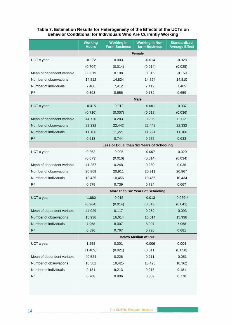
Table 5. Estimation Results of the Effects of the UCTs on Behavior Conditional for Individuals Who Are Currently Working 11

Table 6. Estimation Results for Heterogeneity of the Effects of the UCTs on Behavior 12

Table 7. Estimation Results for Heterogeneity of the Effects of the UCTs on Behavior Conditional for Individuals Who Are Currently Working 14

LIST OF FIGURES Figure 1. The numbers of target beneficiaries and budget allocations for Indonesia’s

unconditional cash transfers over the years 3

Figure 2. Time horizon of IFLS data and cash transfer disbursements 4

LIST OF APPENDICES Appendix 1. Table A1. Estimation Results of the Effects of the UCTs on Behavior Separated for

Datasets 1 and 2 20

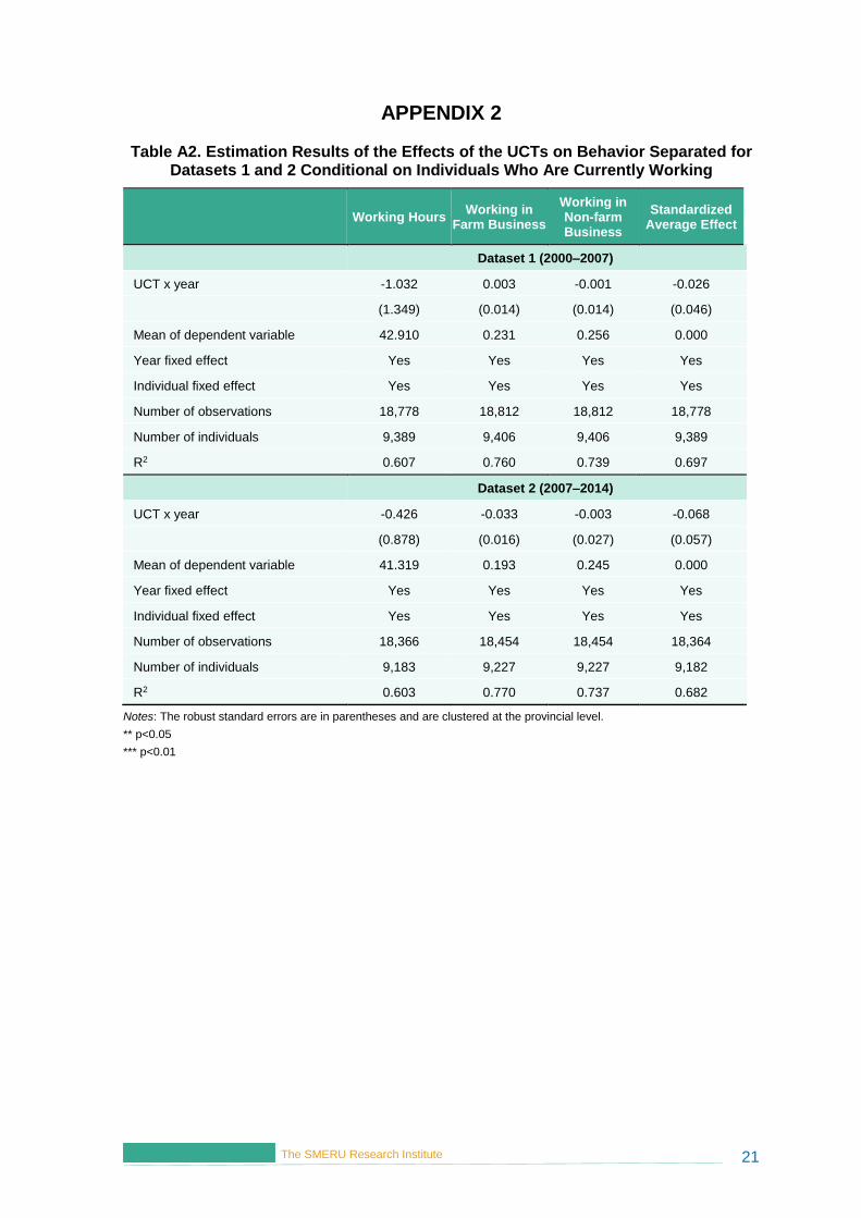
Appendix 2. Table A2. Estimation Results of the Effects of the UCTs on Behavior Separated for Datasets 1 and 2 Conditional on Individuals Who Are Currently Working 21

Appendix 3. Table A3. Additional Results of the Effects of the UCT on Behavior for Dataset 2 22

Appendix 4. Table A4. Estimation Results of the Effects of the UCTs on Behavior Using Share of Transfer as Explanatory Variable 23

Appendix 5. Table A5. Parallel Assumption Test 24

Appendix 6. Figure A1. Changes in the Main Outcomes between Baseline and Endline 25

Appendix 7. Figure A2. Changes in the Main Outcomes between Baseline and Endline for Individuals Who Are Currently Working 26

Appendix 8. Table A6. The Estimation Results of the Effects of the UCTs on Behavior Using District-Level Matching 27

Appendix 9. Table A7. The Estimation Results of the Effects of the UCTs on Behavior Using District-Level Matching Conditional for Individuals Who Are Currently Working 28

Appendix 10. Table A8. The Estimation Results of the Effects of the UCTs on Behavior Using Subdistrict-Level Matching 29

v The SMERU Research Institute

Appendix 11. Table A9. The Estimation Results of the Effects of the UCTs on Behavior Using Subdistrict-Level Matching Conditional for Individuals Who Are Currently Working 30

Appendix 12. Table A10. Estimation Results of the Effects of the UCTs on Behavior for Individuals in the Bottom 40% of Per Capita Expenditure 31

Appendix 13. Table A11. Estimation Results of the Effects of the UCTs on Behavior for Individuals in the Bottom 40% of Per Capita Expenditure (Conditional for Individuals Who Are Currently Working) 32

Appendix 14. Table A12. Estimation Results of the Effects of the UCTs on Behavior for Individuals in the Top 40% of Per Capita Expenditure 33

Appendix 15. Table A13. Estimation Results of the Effects of the UCTs on Behavior for Individuals in the Top 40% of Per Capita Expenditure 34

Appendix 16. Table A14. Statistical Summary of the Combined Sample 35

vi The SMERU Research Institute

LIST OF ABBREVIATIONS

Abbreviations Indonesian English

ARA absolute risk aversion

BDT Basis Data Terpadu Unified Database

BKKBN Badan Kependudukan dan Keluarga Berencana Nasional

National Population and Family Planning Agency

BLSM Bantuan Langsung Sementara Masyarakat

Temporary Direct Cash Transfer

BLT Bantuan Langsung Tunai Direct Cash Transfer

BPS Badan Pusat Statistik Indonesia Statistics

CEM Coarsened Exact Matching

CGE Computable General Equilibrium

DID difference-in-differences

IFLS Survei Aspek Kehidupan Rumah Tangga Indonesia (Sakerti)

Indonesian Family Life Survey

JKN Jaminan Kesehatan Nasional Indonesian National Health Insurance

PDM-DKE Pemberdayaan Daerah dalam Mengatasi Dampak Krisis Ekonomi

Regional Empowerment to Overcome the Impact of the Economic Crisis

PIP Program Indonesia Pintar Scholarship for Students from Poor Households

PKH Program Keluarga Harapan Household Conditional Cash Transfer

PMT proxy means test

PPLS Pendataan Program Perlindungan Sosial

Data Collection for Social Protection Programs

PSE Pendataan Sosial-Ekonomi Socioeconomic Data Collection

PSM Propensity Score Matching

Rastra Beras Sejahtera Rice for the Poor

RCT randomized controlled trial

SKTM surat keterangan tidak mampu financial eligibility statement

Susenas Survei Sosial-Ekonomi Nasional National Socioeconomic Survey

TNP2K Tim Nasional Percepatan Penanggulangan Kemiskinan

National Team for the Acceleration of Poverty Reduction

UCT unconditional cash transfer

1 The SMERU Research Institute

I. INTRODUCTION Governments provide social protection to mitigate adverse impacts of shocks, especially to those who are at risk or have fallen into poverty. Social protection programs are designed such that once a shock is over and the beneficiaries recover, the assistance would cease. An exception to this is the permanent assistance provided to chronically poor individuals, for example, the disabled or elderly. However, receiving government cash transfers could alter the behavior of beneficiaries. Specifically, they could expose themselves to unnecessary risks and do not sufficiently insure themselves. Furthermore, they may participate less in the labor market because they assume that the government would provide cash transfers indefinitely. Evidence from the United States shows that farmers reduce insurance purchases as expectations of government disaster payments increase (Deryugina and Kirwan, 2016). Ashenfelter and Plant (1990) found that households reduce labor supply as subsidies get higher. Kousky, Kerjan, and Raschky (2014) used a panel dataset from Florida and showed that increases in federal post-disaster assistance grants significantly decrease individual insurance coverage. Raschky and Schwindt (2009) estimated the impact of foreign aid on the beneficiary country's preparedness against natural disasters and found that increases in the level of past foreign aid imply higher death tolls resulting from natural disasters. This result implies that foreign aid in previous periods provided perverse incentives in terms of a country’s effort to provide protective actions for their citizens. In contrast to these findings, Banerjee et al. (2017) found no statistically significant effects of receiving cash transfers on employment. They summarized RCT studies conducted in six countries, including those on Indonesia’s conditional cash transfer program, and used working status and working hours as outcome variables. Also related to labor market outcome, Bosch and Schady (2019) used regression discontinuity design and found that Ecuador welfare payments did not reduce labor supply over a five-year period. Marinescu (2018) also found no statistically significant effects of receiving cash transfers on employment. Furthermore, this study finds positive effects of cash transfers on health and education outcomes, while decreasing criminality as well as drug and alcohol use. Looking specifically at Native American children, Akee et al. (2018) found positive effects of unconditional cash transfers on behavioral and personality traits. Meanwhile, Handa et al. (2018) evaluated a large-scale government unconditional cash transfer in Sub-Saharan Africa. Findings from their investigation reject the perception regarding negative effects of the cash transfer that (i) it induces higher spending on alcohol or tobacco; (ii) it is fully consumed rather than invested; (iii) it creates dependency, for example, by reducing participation in productive work; (iv) it increases fertility; (v) it leads to negative community-level economic impacts (including price distortion and inflation); and (vi) it is fiscally unsustainable. Similarly, Evans and Popova (2017) reviewed 19 studies on the effects of cash transfers on expenditure on temptation goods. Overall, they found a negative and significant effect. In summary, the literature provides mixed results on the behavioral effects of government cash transfer programs. In Indonesia, after a shock due to fuel subsidy reduction in late 2005, the government implemented a large unconditional cash transfer (UCT) program called BLT (Bantuan Langsung Tunai, or Direct Cash Transfer) to mitigate the impacts. Yusuf and Resosudarmo (2008) used Computable General Equilibrium (CGE) modelling and found all households to be affected by the fuel subsidy reform,


although the richer households are more impacted. They found that BLT could compensate the poor from higher prices induced by the fuel subsidy reduction, especially in rural areas. While some of the poorest urban poor gain positive (nominal) income because of the transfer, the net real expenditure effect is still negative. On the other hand, a study by Bazzi, Sumarto, and Suryahadi (2015) evaluates the implementation of BLT and shows that a timely receipt of a cash transfer is important for consumption smoothing. They found that there is no difference on per-capita expenditure growth between beneficiaries and nonbeneficiaries if a cash transfer is received timely. However, a delayed receipt reduces expenditures of beneficiaries by 7.5 percentage points. In this paper, we estimate the behavioral effects of BLT and its successor, BLSM (Bantuan Langsung Sementara Masyarakat, or Temporary Direct Cash Transfer), which was implemented in 2013. BLT and BLSM had about 15.5 million beneficiary households each. The program1 remains one of the largest cash transfer programs in the world. We use a wide range of outcomes, from smoking to insurance purchase and labor market participation. We also test the effects of the cash transfers to risk aversion and time preferences. We find no evidence that receiving the unconditional cash transfer program changes the behavior of the beneficiaries. We also find no evidence of effect heterogeneity by sex, education level, and level of welfare. Therefore, our results add to the literature that finds no evidence of unintended behavioral effects of cash transfers. We organize the rest of the paper as follows. The next section provides further information on the unconditional cash transfers in Indonesia. Section 3 presents the estimation strategy. Section 4 discusses the findings. Section 5 concludes.

II. INDONESIA’S UNCONDITIONAL CASH TRANSFERS

Introduced in the last quarter of 2005, Indonesia’s first unconditional cash transfer was intended to reduce the impact of a fuel subsidy reduction—hence an increase in domestic fuel prices—by reallocating the budgetary savings as direct benefit given to poor and vulnerable households which were most at risk from induced general price increases (World Bank, 2017). The fuel subsidy reduction was necessitated by a steep increase in international oil prices that, given the fixed domestic fuel prices, caused ballooning fuel subsidy in the government budget. At the beginning, the program, which was called BLT, was targeted at the poorest 30% of households. The initial program ran for one year, until September 2006. It was later re-implemented several times intermittently whenever the government reduced fuel subsidies and consequently increased domestic fuel prices. Figure 1 shows the years the unconditional cash transfers were implemented as well as the number of beneficiaries and the amount of budget allocated for each year. In 2005/2006 (BLT I), there were initially 15.4 million beneficiary households before an increase to 18 million households. They received a transfer of Rp1.2 million for one year, provided on a quarterly basis (Rp300,000 per three month). That benefit is around 15% of the quarterly expenditures for the average beneficiary (Bazzi, Sumarto, and Suryahadi, 2015). In 2008/2009 (BLT II), another cash transfer was made by the government to respond to the global financial crisis. This time, the cash transfer targeted 19 million

1The program refers to both BLT and BLSM, two similar unconditional cash transfers that were implemented in different years and with different targeting schemes (see Section II).


households. The amount of benefit was the same at Rp100,000 per month, but only provided to cover nine months (Rp900,000 in total per household). The cash transfer was again made in 2013 under a different name (BLSM) for a few months. In 2014/2015, the government eliminated the fuel subsidy to relieve the national budget and as the consequence, another transfer of Rp150,000 per month was made to 15.5 million people for several months. However, the BLSM in 2014/2015 had a lower total benefit compared to BLT in 2005/2006.

Figure 1. The numbers of target beneficiaries and budget allocations for Indonesia’s unconditional cash transfers over the years Source: World Bank, 2017.

III. EMPIRICAL ESTIMATION STRATEGY

3.1 Data We use four rounds of the Indonesian Family Life Survey (IFLS)2: 1997, 2000, 2007, and 2014. IFLS is a large ongoing longitudinal household survey in Indonesia, representative of 83% of the Indonesian population (Strauss, Witoelar, and Sikoki, 2016). The first wave, conducted in 1993, consisted of over 30,000 individuals in about 7,000 households in 13 of 27 provinces. The second and third waves were conducted in 1997 and 2000, respectively. The same household respondents were re-interviewed in late 2007 as part of IFLS wave 4 and in late 2014 as IFLS wave 5. The IFLS has a low attrition rate. Strauss, Witoelar, and Sikoki (2016) claimed that 92% of households that were interviewed in 1993 were successfully re-interviewed in all subsequent rounds. The IFLS has a specific module related to social assistance programs in Indonesia (KSR Section of Book 1). The module has similar questions in the last three rounds that we analyze. We use the

2IFLS is publicly available at https://www.rand.org/labor/FLS/IFLS.html.

4,487

18,619

13,966

3,733

9,300

6,200

9,470

15.4

1819 19

15.5 15.5 16

0

2

4

6

8

10

12

14

16

18

20

0

2,000

4,000

6,000

8,000

10,000

12,000

14,000

16,000

18,000

20,000

2005 2006 2008 2009 2013 2014 2015

(mill

ion

ho

use

ho

lds)

(bill

ion

ru

pia

h)

Government budget (LHS) The number of target beneficiaries (RHS)


questions on the unconditional cash transfers from the government. Figure 2 shows the time horizon of IFLS data and cash transfers in Indonesia. IFLS wave 3 was conducted in late 2000. From the dataset, only about 27 households (or 0.3% out of the total households) indicated that they have ever received an unconditional cash transfer.3 Coincidentally, the last two survey rounds (2007 and 2014) coincided with the years the largest unconditional cash transfer program was being implemented. The IFLS wave 4, conducted between late 2007 and early 2008, recorded the beneficiaries of BLT. There were 2,771 households (or 22% out of the total households) that received BLT I in IFLS wave 4 and only 2% of those households that received BLT 2008 (BLT II) because IFLS wave 4 was being enumerated until mid-2008. Meanwhile, IFLS wave 5, conducted between late 2014 and early 2015, recorded the beneficiaries of BLSM. There were 1,800 households (12% out of the total households) that received BLSM in IFLS wave 5. There were 60% of households that received BLSM and ever received BLT II in 2008.

Figure 2. Time horizon of IFLS data and cash transfer disbursements

Regarding the targeting of the unconditional cash transfer program, BLT 2005 used PSE (Pendataan Sosial-Ekonomi, or Socioeconomic Data Collection) 2005 database as the targeting tool. PSE 2005 is a survey that was conducted by Statistics Indonesia (Badan Pusat Statistik or BPS). BPS collected data on the socioeconomic characteristics of poor households listed through interviews with village heads and community leaders. The household list was crosschecked with other poverty information sources, such as BKKBN4 data and poverty surveys conducted by the provinces. The PSE 2005 survey collected 14 nonmonetary variables to use in measuring the welfare of the households. BPS then used a proxy means test (PMT) to determine the eligibility of beneficiaries. Based on the PMT result, 19.1 million households were recorded in the PSE 2005 as extreme poor, poor, or near poor. A similar survey was also conducted in 2008 for targeting households for the disbursement of BLT 2008 program (BLT II). The survey was called PPLS (Pendataan Program Perlindungan Sosial, or Data Collection for Social Protection Programs) 2008. The survey’s process and method were similar to those of PSE 2005. The PPLS then expanded to PPLS 2011 or BDT (Basis Data Terpadu, or Unified Database) 2011, but with some improvements in its method and sampling frame (TNP2K, 2015). BDT 2011 was also conducted by BPS. BDT 2011 used Population Census 2010 as the baseline data. BDT 2011 collected more variables than PSE 2005. In total, BDT 2011 surveyed 45% of households in Indonesia compared to only 29% in PSE 2005. It means that BDT 2011 also covered nonpoor but

3This is likely from PDM-DKE (Pemberdayaan Daerah dalam Mengatasi Dampak Krisis Ekonomi, or Regional Empowerment to Overcome the Impact of the Economic Crisis), a social safety net program during the Asian Financial Crisis which provided block grants to communities. Some communities had used the grants to provide cash transfers to poor households.

4BKKBN or Badan Kependudukan dan Keluarga Berencana Nasional is the National Population and Family Planning Agency.

1998–1999 2000 2005–2006 2007–2008 2013–2014 2014–2015

Asian Financial Crisis

IFLS wave 3

IFLS wave 4

IFLS wave 5

BLSM disbursement

BLT disbursement


considered vulnerable households. The BDT database is the embryo of the unified database used by many social protection programs in Indonesia in the last decade.

3.2 Matching Process We aim to estimate the effect of receiving BLT and BLSM on individual attitude and behavior. The identification challenge pertains to the fact that BLT and BLSM were not randomly assigned. It targeted the poorest households. Hence, we need to circumvent the selection bias. To identify the effects of BLT, we use the nonbeneficiary households that have observably similar preprogram characteristics as a control group. Practically, these households were the ones that suffer from undercoverage; they should have received the program but for some reason did not. Like many targeted social assistance programs in other countries, the unconditional cash transfer program in Indonesia also contains targeting error5, which includes undercoverage (or exclusion error) and leakage (or inclusion error). Using Susenas (Survei Sosial-Ekonomi Nasional, or National Socioeconomic Survey; the official annual household socioeconomic survey) data, we calculate the exclusion and inclusion errors for BLT I, BLT II, and BLSM. The exclusion errors for BLT I, BLT II, and BLSM are 47%, 54%, 66%, respectively. Meanwhile, their inclusion errors are 21%, 18%, and 12%, respectively. The exclusion and inclusion errors for BLT and BLSM are relatively comparable with similar programs in other developing countries (Sumarto and Bazzi, 2011). To estimate the effects of the unconditional cash transfers on behavior, we prepare our data in the following manner. The first dataset is an individual-level longitudinal dataset from IFLS 2000 and 2007. The former covers pre-BLT I, while the latter post-BLT I. The second dataset is also an individual-level longitudinal dataset, created from IFLS 2007 and 2014. It covers the pre- and post-BLT II and BLSM. We show the comparative statistics on a set of household and individual characteristics between cash transfer beneficiaries (treatment group) and nonbeneficiaries (control group) for these two datasets separately in Table 1. The comparison shows that the beneficiaries have lower education, are poorer, reside mainly in rural areas, and have lower access to safe drinking water and proper sanitation compared to nonbeneficiaries in the initial year. In addition, they have a higher proportion of both receiving a cash transfer and having a surat miskin6 in the initial year. Almost all covariates that we test are significantly different. Note that the nonbeneficiaries in this table covers both the poor who were supposed to receive the program but did not, and the nonpoor who were not supposed to receive the program. On the other hand, the beneficiaries also comprised the poor who were supposed to receive the program and the nonpoor who were not supposed to receive the program but did. In order to balance the characteristics of the treatment and control groups, we then match the pre-BLT characteristics between the beneficiaries and nonbeneficiaries based on the BLT beneficiary status in 2007 using Coarsened Exact Matching (CEM). We prefer to use CEM because the method requires fewer assumptions, is more easily automated, and possesses more attractive statistical properties for many applications than Propensity Score Matching (PSM) or any other matching

5Undercoverage or exclusion error in this paper is defined as the proportion of households that were eligible but did not receive the program. Meanwhile, leakage or inclusion error is defined as the proportion of households that were not eligible but received the program. The targeting figure we get for BLT and BLSM has a similar pattern with other programs, such as Rastra (Rice for the Poor), PKH (Household Conditional Cash Transfer), and PIP (Scholarship for Students from Poor Households). See Rahayu et al. (2018) for further review.

6Surat miskin or surat keterangan tidak mampu (SKTM) is a financial eligibility statement issued by the village office.


method (Blackwell et al., 2009). The matching aims to improve the estimation of causal effects by removing the imbalance in pretreatment covariates between the treatment and control groups (Iacus, King, and Porro, 2012). Finally, CEM calculates sample weights, which we use in the regressions.

Table 1. Prematching Characteristics in the Initial Year Based on UCTs

Beneficiary Status

Variables

Characteristics in 2000 for Treatment in 2007

(Dataset 1)

Characteristics in 2007 for Treatment in 2014

(Dataset 2)

Mean of Control Group

Difference to Treatment

Group p-value

Mean of Control Group

Difference to Treatment

Group p-value

Poor status (yes=1) 0.11 0.16 0.00 0.04 0.08 0.00

Ever received cash transfer (yes=1) 0.01 0.01 0.00 0.19 0.29 0.00

Having card for the poor (yes=1) 0.05 0.04 0.00 0.10 0.10 0.00

Female (yes=1) 0.53 0.02 0.00 0.53 0.01 0.18

No schooling (yes=1) 0.08 0.12 0.00 0.07 0.03 0.00

Primary schools (yes=1) 0.37 0.18 0.00 0.34 0.20 0.00

Junior secondary schools (yes=1) 0.17 -0.02 0.00 0.18 0.03 0.00

Senior secondary schools (yes=1) 0.28 -0.18 0.00 0.30 -0.15 0.00

University (yes=1) 0.09 -0.09 0.00 0.11 -0.10 0.00

Other schools (yes=1) 0.01 0.00 0.12 0.01 0.00 0.96

House ownership (yes=1) 0.80 0.04 0.00 0.77 0.02 0.00

Safe drinking water (yes=1) 0.88 -0.05 0.00 0.76 0.03 0.00

Own toilet with septic tank (yes=1) 0.56 -0.30 0.00 0.68 -0.22 0.00

Having land for farming (yes=1) 0.37 0.00 0.93 0.33 -0.06 0.00

Urban residence (yes=1) 0.52 -0.18 0.00 0.52 -0.07 0.00

Note: The number of observations in 2000 is 16,587 for the control group and 5,117 for the treatment group. Meanwhile, the number of observations in 2007 is 22,076 for the control group and 3,443 for the treatment group. The mean difference estimation is conducted by using simple regression that estimates the characteristics in the initial year as listed above to the unconditional cash transfer status in the treatment year.

We match between cash transfer beneficiary households and nonbeneficiary households with similar characteristics. As a rich dataset, IFLS allows us to control for a set of socio-demographic characteristics in the baseline. Specifically, for Dataset 1, we match individual characteristics in 2000 using the unconditional cash transfer status in 2007. Similarly, for Dataset 2, we match individual characteristics in 2007 using the unconditional cash transfer status in 2014. We use the variables from Bazzi, Sumarto, and Suryahadi (2015) for the matching. These variables significantly affect the likelihood of households to receive the unconditional cash transfers. The main characteristics that we match are the poverty status, ever received social assistance in cash, and having surat miskin in the baseline year. We also match on more individual and household characteristics: sex, education level, housing status, drinking water sources, sanitation, land ownership, and urban status in the baseline year. Those variables capture the aspects of poverty. More deprived individuals in all those aspects have a higher probability to receive the cash transfers


in the treatment years. We also control for regional heterogeneity by including province fixed effects in the matching equation. Note that since behavioral variables are measured at the individual level, while cash transfer receipt is measured at the household level, we include all adults in the households. As such, we assume that all household members benefit from the unconditional cash transfers. Table 2 shows the CEM summary. Our matched dataset contains 13,155 nonbeneficiary individuals and 4,631 beneficiary individuals for Dataset 1, a total of 17,786 individuals out of the initial total sample of 21,704 individuals. Meanwhile, for Dataset 2, we match 13,985 nonbeneficiary individuals and 2,920 beneficiary individuals with a total of 16,905 individuals. We use these observations in our estimations. From the final sample, as many as 26% and 17% of individuals were exposed to the unconditional cash transfers in both datasets, respectively.

Table 2. Coarsened Exact Matching Summary

Dataset 1 (2000–2007) Dataset 2 (2007–2014)

Nonbeneficiaries Beneficiaries Total

Nonbeneficiaries Beneficiaries Total

(UCT=0) (UCT=1) (UCT=0) (UCT=1)

All 16,587 5,117 21,704 22,076 3,443 25,519

Matched 13,155 4,631 17,786 13,985 2,920 16,905

Unmatched 3,432 486 3,918 8,091 523 8,614

In Table 1, before matching, the multivariate imbalance (L1) 7 is 0.56. After matching, the multivariate imbalance decreases considerably to 0.15 for both datasets. Similarly, the imbalance of each covariate also decreases significantly. Since CEM ensures baseline balance between the treatment and control groups, we do not show the postmatching balance.

3.3 Difference-in-Differences (DiD) Estimation After matching, we estimate a difference-in-differences model as follows: 𝑏𝑒ℎ𝑎𝑣𝑖𝑜𝑟𝑖𝑡 = 𝛼 + 𝛽𝑈𝐶𝑇𝑖𝑡 × 𝑡𝑖𝑡 + 𝜃𝑡𝑖𝑡+ 𝛿𝑖 + 휀𝑖𝑡 (1)

where 𝑏𝑒ℎ𝑎𝑣𝑖𝑜𝑟𝑖𝑡 is the behavior of individual i in year t; 𝑈𝐶𝑇𝑖𝑡 is the unconditional transfer beneficiary status of the household; 𝑡𝑖𝑡 is the year dummy (treatment year = 1); 𝜃 is the time effect that captures the outcome differences across time; 𝛿𝑖 is the individual fixed effect to control time-invariant unobserved heterogeneity of individuals; and 휀𝑖𝑡 is the error term. The interaction variable 𝑈𝐶𝑇𝑖𝑡 × 𝑡𝑖𝑡 is the variable of interest which captures the effect of the program, while 𝛽 is the magnitude of the effect. Meanwhile, 𝛼 is the constant term which shows the mean of the outcome of the control group in the initial period. By combining matching and difference-in-differences using fixed-effect estimation, our identifying assumption is that once observable differences and time-invariant unobserved heterogeneity are considered, no more sources of bias are present.

7L1 is an indicator in CEM that shows the multivariate imbalance test result with a value ranging from 0 (balance) to 1 (imbalance).


We estimate Datasets 1 and 2 together as a combined dataset. To control the outcome difference across datasets, we add a dummy which indicates the dataset. 8 We also estimate model (1) separately for Datasets 1 and 2. To further test the common trends assumption, we conduct placebo estimations. We estimate model (1) using the previous period. For Dataset 1, we use IFLS 1997 and 2000. For Dataset 2, we use 2000 and 2007 data.

3.4 Behavioral Indicators The outcome variables come from the individual-related questionnaires contained in Books 3A and 3B of IFLS. Those modules were answered by household members who were 15 years old and older. Table 3 shows the behavioral indicators that we include as outcome variables. The more risky behavior is indicated by the negative direction of the indicators. Risk aversion is indicated in the opposite direction. We include arisan membership as a behavioral indicator. Arisan is a rotating savings group (also known as RoSCA), an informal community gathering that involves a money saving activity across members. Value of 1 means that the individual has joined an arisan in the past year and 0 means otherwise. Following Brunette et al. (2013), we use this variable to examine whether receiving a government cash transfer reduces membership in informal insurance. We define smoking behavior as an individual who (i) is currently not smoking or has totally stopped chewing tobacco, (ii) is not smoking a pipe or self-rolled cigarettes, or (iii) is not smoking cigarettes/cigars (1=yes, 0=otherwise). We construct the variable this way to ensure that in all our dependent variables, a positive answer is a good outcome. The medical checkup variable means that an individual has ever checked his/her health at a medical facility in the last five years. Ownership of a private insurance is defined as an individual who holds a private insurance or savings-related insurance. We exclude the ownership of social insurance, such as the Indonesian National Health Insurance (Jaminan Kesehatan Nasional or JKN), which is fully subsidized by the government. Working status is positive for individuals who worked at least one hour in the previous week, or the individual has a job but is temporarily not working in the past week. We define the working hour variable as the total number of hours worked in the last week. Since workers in Indonesia (especially the poor) mostly work in the agricultural or informal sector, and have a high likelihood of having multiple jobs, we sum all the working hours of the workers for both the main job and additional jobs. Meanwhile, the variable working in a farm business is defined as a dummy variable taking the value of 1 if the individual is working in a farm business and 0 if otherwise. Similarly, the variable working in a nonfarm business is also a dummy variable that is equal to 1 for an individual who is working in a nonfarm business. We define the farm and nonfarm business activities when an individual is working in the agricultural and nonagricultural sectors, respectively, but with the type of job either self-employed, self-employed with unpaid family workers/temporary workers, or self-employed with permanent workers. For the indicators related to labor market (working hours, and farm and

8Technically, we modify model (1) and estimate: 𝑏𝑒ℎ𝑎𝑣𝑖𝑜𝑟𝑖𝑡 = 𝛼 + 𝛽𝑈𝐶𝑇𝑖𝑡 × 𝑡𝑖𝑡 + 𝜃𝑡𝑖𝑡+ 𝛿𝑖 + 𝜕𝑑 + 휀𝑖𝑡. Variable 𝜕𝑑 is a dummy that has the value of 1 for Dataset 2 and 0 for Dataset 1.


nonfarm business activities), we estimate the effect exclusively for individuals who are currently working only during the survey round.

Table 3. Behavioral Indicators

Variable Description

Main Outcome

Participate in an arisan group (rotating savings group)

Have you participated in arisan in the last 12 months? (Yes=1, 0=otherwise)

Currently not smoking (quit smoking or never smoke)

Are you currently not smoking or have you totally quit smoking? (Yes=1, 0=otherwise)

Having medical check Have you had a general checkup performed in the last 5 years? (Yes=1, 0=otherwise)

Having private insurance Private insurance or benefits ownership (Yes=1, 0=otherwise)

Currently working During the past week, did you work to get paid? (Yes=1, 0=otherwise)

Working hours in the past week

What was the total number of hours you worked during the past week (on your job)? (in hours)

Working in farm business Working in farm business (Yes=1, 0=otherwise)

Working in nonfarm business Working in nonfarm business (Yes=1, 0=otherwise)

Outcomes Only Available in IFLS 2007 and 2014

Hypothetical risk aversion Absolute risk aversion (ARA) index, higher index means more risk averse (value 0.005 to 0.250)

Hypothetical time preference Time preference index, higher index means more patience (value 1 to 5)

Additionally, we also use risk and time preferences as outcome variables. We use the preferable index of measuring hypothetical risk question, which is the Arrow-Pratt index, as a measure of absolute risk aversion (ARA) (Sanjaya, 2013). A higher ARA index means higher risk aversion. Meanwhile, the time preference variable is constructed with values ranging from 1 to 5. A larger value of time preference means that an individual is more patient. In total, we have eight different main outcome variables divided into two groups. The first group contains variables that apply to all individuals. The second group contains variables that apply only to working individuals. To avoid overemphasizing and cherry-picking the result, we follow Kling, Liebman, and Katz (2007) to estimate the average effect of treatment to outcomes. For this purpose, we create an index of risk behavior called summary index that averages together the five measures of risky behavior for all sample and three measures for working individuals. The summary index is defined such that more beneficial outcomes have higher scores. It is defined as z-scores that are calculated by subtracting each outcome with control group mean and then dividing the result with the control group standard deviation. After that, we average all the normalized z-scores of the variables and then standardize the average relative to the control group. Therefore, the value of index has an average of 0 with a standard deviation of 1 for the control group. We present findings from this summary index which aggregate information over all treatment effects to draw a general conclusion. Because it is in z-score, the summary index is known as standardized average effect.


IV. ESTIMATION RESULTS

4.1 Behavioral Effects of Receiving the Unconditional Cash Transfers

Table 4 and Table 5 show the main results9 on the effects of receiving the unconditional cash transfers on individual behavior. We find no evidence that an unconditional cash transfer receipt affects behavior. We can also rule out large effects. The coefficients of participation in arisan, smoking behavior, medical checkup, ownership of a private insurance, and working status are all statistically insignificant and almost zero. Similarly, among those who are working, receiving the unconditional cash transfers has no statistically significant effects on working hours in the past

week and activities in a farm or nonfarm business. The last columns of Table 4 and Table 5 show the standardized average effects of receiving the unconditional cash transfers that confirm our findings, both of which are not statistically significant.

Table 4. Estimation Results of the Effects of the UCTs on Behavior

Participate in Arisan

Quit Smoking

/Never Smoke

Having Medical

Checkup

Having Private

Insurance

Currently Working

Standardized Average

Effect

UCT x year -0.006 -0.001 -0.003 -0.002 0.007 -0.008

(0.008) (0.005) (0.006) (0.001) (0.009) (0.018)

Mean of dependent variable

0.260 0.661 0.092 0.004 0.744 0.000

Year fixed effect Yes Yes Yes Yes Yes Yes

Individual fixed effect

Yes Yes Yes Yes Yes Yes

Dataset fixed effect Yes Yes Yes Yes Yes Yes

Number of observations

61,540 61,588 59,500 69,382 61,714 59,494

Number of individuals

30,770 30,794 29,750 34,691 30,857 29,747

R2 0.645 0.889 0.501 0.463 0.627 0.620

Notes: Estimation results from this table include two datasets that combined Dataset 1 (matching 2000–2007) and Dataset 2 (matching 2007–2014). The robust standard errors are in parentheses and are clustered at the provincial level.

** p<0.05

*** p<0.01

APPENDIX 1 and APPENDIX 2 show the main estimation results separated for Datasets 1 and 2. The results are similar. APPENDIX 3 shows the additional estimation results for Dataset 2 that estimate the effects of the unconditional cash transfer on risk aversion index and time preference index. The results are also similar with our main findings. The coefficient is almost zero and insignificant for the three indicators.

9The estimation results that are shown in the tables are estimated from model (1). For convenience, we only show coefficient β from the interaction of the unconditional cash transfer status and year dummy in the first row. Meanwhile, the mean of dependent variable is calculated using the mean of the outcome of the control group (see APPENDIX 16).


One possible reason for these findings is that the amount of the cash transfers received by the households is too small, around 15% of the total expenditure (Bazzi, Sumarto, and Suryahadi, 2015). To test this possibility, instead of using the beneficiary status dummy of the cash transfer, we estimate model (1) using the cash transfers received as a proportion of the annual household expenditure. The IFLS questionnaire also includes the amount of benefit received by the beneficiary households. The results are shown in APPENDIX 4. We find similarly statistically insignificant estimates, except for two outcomes: participation in arisan and ownership of a private insurance. However, the average effects of the treatment in the last column still show insignificant results.

Table 5. Estimation Results of the Effects of the UCTs on Behavior Conditional for

Individuals Who Are Currently Working

Working

Hours Working in Farm

Business Working in Non-farm Business

Standardized Average Effect

UCT x year -0.260 -0.006 -0.006 -0.033

(0.513) (0.007) (0.011) (0.027)


42.081 0.211 0.250 0.000

Year fixed effect Yes Yes Yes Yes

Individual fixed effect Yes Yes Yes Yes

Dataset fixed effect Yes Yes Yes Yes

Number of observations 37,144 37,266 37,266 37,142

Number of individuals 18,572 18,633 18,633 18,571

R2 0.555 0.735 0.705 0.652


** p<0.05

*** p<0.01

Our main findings are in line with the findings of Banerjee et al. (2017) in six developing countries, including Indonesia, in that unconditional cash transfers have a limited effect on behavior. It is also similar to the findings of Marinescu (2018) in the context of a developed country.

4.2 Heterogeneity Analysis Table 6 and Table 7 show the results of effect heterogeneity analyses based on sex, education level, and median consumption expenditure. Table 6 shows that among females and males, the unconditional cash transfers have no significant effects on risky behavior. To avoid endogeneity concerns, we use the initial year level of per-capita household expenditure to separate individuals into below and above the median. Among individuals living in households with per-capita expenditures below the median, we find no effect of the cash transfers on behavior. This is also the case among individuals living in households above the median except for participating in arisan. Individuals who are exposed to the unconditional cash transfers and living in households above the median are 3.3 percentage points less likely to participate in arisan compared to nonbeneficiary individuals. However, the average effect is not significant.


Examining the effect heterogeneity based on education level, we find that the cash transfers decrease probability to not smoke by 1.7 percentage points for individuals with a high education level. However, this is a small effect compared to the mean being that 65% of the individuals from this group are currently not smoking. Despite that, the average effects of the treatment for the high-education group are not significant. Similar to the overall findings, the effects of the unconditional cash transfers on behavior for the group with low levels of education are almost zero and not statistically significant.

Table 6. Estimation Results for Heterogeneity of the Effects of the UCTs on

Behavior


Quit Smoking/

Never Smoke

Having Medical Check

Having Private

Insurance

Currently Working


Effect

Female

UCT x year -0.015 0.005 -0.003 -0.001 0.016 0.003

(0.012) (0.005) (0.007) (0.001) (0.012) (0.021)

Mean of dependent variable 0.346 0.959 0.088 0.003 0.622 0.229

Number of observations 33,869 33,897 32,925 37,534 33,973 32,923

Number of individuals 16,935 16,949 16,463 18,767 16,987 16,462

R2 0.634 0.749 0.493 0.459 0.596 0.588

Male

UCT x Year 0.007 -0.009 -0.004 -0.003 -0.004 -0.023

(0.007) (0.008) (0.008) (0.002) (0.012) (0.022)

Mean of dependent variable 0.150 0.280 0.097 0.005 0.900 -0.295



R2 0.611 0.776 0.511 0.466 0.554 0.591

Less or Equal than Six Years of Schooling

UCT x year -0.006 0.003 -0.002 -0.000 0.006 0.001

(0.009) (0.007) (0.005) (0.000) (0.012) (0.021)




R2 0.670 0.899 0.514 0.462 0.644 0.656

More than Six Years of Schooling

UCT x year -0.010 -0.017*** -0.004 -0.005 0.009 -0.036

(0.015) (0.005) (0.012) (0.003) (0.017) (0.045)




R2 0.648 0.889 0.550 0.492 0.663 0.628



Quit Smoking/

Never Smoke

Having Medical Check

Having Private

Insurance

Currently Working


Effect

Below Median of PCE

UCT x year 0.002 0.001 -0.007 -0.001 0.009 -0.005

(0.009) (0.006) (0.008) (0.001) (0.011) (0.023)




R2 0.656 0.893 0.501 0.527 0.631 0.639

Above Median of PCE

UCT x year -0.033** -0.002 0.004 -0.003 -0.011 -0.037

(0.015) (0.007) (0.013) (0.002) (0.014) (0.021)




R2 0.663 0.896 0.526 0.462 0.659 0.618


Individual fixed effect Yes Yes Yes Yes Yes Yes

Dataset fixed effect Yes Yes Yes Yes Yes Yes


** p<0.05

*** p<0.01

Meanwhile, Table 7 shows the estimation results conditional for only individuals who are currently working. We find no significant effects of the unconditional cash transfers on behavior almost for all subsample categories. There is a statistically significant effect for the variable ‘standardized average effects’ for individuals with more than six years of schooling related to working behavior. This effect is contributed by the negative effect for the variable ‘working status in nonfarm business’; however, it is only weakly significant. Meanwhile, the other two variables in the same row are not statistically significant.


Table 7. Estimation Results for Heterogeneity of the Effects of the UCTs on Behavior Conditional for Individuals Who Are Currently Working

Working

Hours Working in

Farm Business Working in Non-farm Business


Female

UCT x year -0.172 0.003 -0.014 -0.028

(0.704) (0.014) (0.014) (0.025)

Mean of dependent variable 38.319 0.108 0.315 -0.159



R2 0.593 0.656 0.732 0.659

Male

UCT x year -0.315 -0.012 -0.001 -0.037

(0.710) (0.007) (0.013) (0.036)

Mean of dependent variable 44.720 0.283 0.205 0.112



R2 0.513 0.744 0.672 0.633

Less or Equal than Six Years of Schooling

UCT x year 0.262 -0.005 -0.007 -0.020

(0.673) (0.010) (0.014) (0.034)




R2 0.578 0.739 0.724 0.667

More than Six Years of Schooling

UCT x year -1.880 -0.015 -0.013 -0.089**

(0.964) (0.014) (0.013) (0.041)




R2 0.596 0.767 0.726 0.681

Below Median of PCE

UCT x year 1.258 0.001 -0.006 0.004

(1.409) (0.021) (0.011) (0.058)




R2 0.708 0.806 0.809 0.770


Working

Hours Working in

Farm Business Working in Non-farm Business


Above Median of PCE

UCT x year -1.003 -0.016 -0.020 -0.083

(1.532) (0.019) (0.028) (0.059)




R2 0.784 0.878 0.846 0.827



Dataset fixed effect Yes Yes Yes Yes


** p<0.05

*** p<0.01

APPENDIX 5 shows the estimation results for the placebo test. All the coefficients are almost zero and not significant, which indicates that there is no significant difference of the outcome before the treatment period.

V. ROBUSTNESS CHECK Some studies show that cash transfers have a spillover on the behavior of nonbeneficiaries. Angelucci and De Giorgi (2009) found a positive spillover. Not only that, a Mexican welfare program, Progresa, has a positive impact on consumption of the beneficiaries, but also a positive impact on the consumption of the ineligible households in the same treated villages. They showed that a cash injection into a group of households affects all families living in the same village. The mechanism behind the indirect effects of Progresa is that the ineligible households living in the treated villages receive more informal loans, receive more transfers from family and friends, and reduce their livestock and grains. Meanwhile, Baird, de Hoop, and Özler (2013) found a negative spillover of cash transfers. They found that while cash transfers strongly reduced psychological distress among schoolgirls, there was also strong evidence of increased psychological distress among untreated schoolgirls in the treatment areas. The effects dissipated soon after the program ended. Considering this, we need to examine whether our findings emerge due to a spillover. Consider a person who is supposed to receive BLT/BLSM but did not. The person then sees that her/his neighbor receives it. That event could change his/her behavior, for example, by stopping working due to disappointment, or taking up more smoking. Since the treatment effects are all zero, the only way a spillover could cause this is when the risky behavior of the control group changes in the same direction as that of the treatment group. We check whether this is the case. APPENDIX 6 and APPENDIX 7 show the changes in our main


outcomes and confirm that there is no significant change between baseline and endline in the control group. Second, spillovers are more likely to happen between neighbors, whereas our matching takes place at the provincial level. However, we check whether our results are different when we match treatment and control groups in a smaller area (such as the district or subdistrict level). The estimation results are shown in APPENDIX 8 to APPENDIX 11. Except the variable ‘having private insurance’ in the subdistrict-level matching, all the effects for the other variables are not statistically significant. The standardized average effects confirm our estimation that the effects are practically close to zero. Third, the spillover could be a function of baseline expenditure levels. When richer people see that their equally rich neighbors get BLT/BLSM, the spillover would likely be smaller compared to when poor people see that their equally poor neighbors get BLT. So, the next robustness check is that we test the impact heterogeneity for the bottom 40% and top 40% of expenditures at baseline. The estimation results are shown in APPENDIX 12 to APPENDIX 15. We find no effect of the unconditional cash transfer on almost all outcomes for both expenditure groups. There is one significant result, that is, the effect for the variable ‘standardized average effects’ for the sample in top 40% related to working behavior, similar to the estimation result for individuals with more than six years of schooling. This effect is also contributed by the negative effect for the variable ‘working status in nonfarm business’; however, it is only weakly significant. In conclusion, our estimates are unlikely to contain spillover bias.

VI. CONCLUSION Cash transfers are currently a widely used tool in the portfolio of social protection programs in many developing countries. This was spurred by evidence which shows that cash transfers are effective in reducing poverty, increasing educational attainment, and improving health status of the poor. However, due to behavioral effects among the beneficiaries, cash transfers can have potential adverse outcomes, such as reduced labor market participation, reduced economic activity, lack of insurance or savings, or increased risky health behaviors, such as smoking. In this paper, we empirically examine the behavioral effects of a large-scale unconditional cash transfer program in Indonesia. The unconditional cash transfer program targeting poor households in Indonesia began in 2005 to mitigate the impact of increasing fuel prices. Over the course of a decade, the program had been implemented intermittently whenever the government raised fuel prices. Covering between 15 up to 19 million households, Indonesia’s unconditional cash transfer program is one of the largest of such programs in the world. To examine the behavioral effects of this program, we use a wide range of outcomes of risk indicators, from smoking habit to insurance purchase and labor market participation. Our estimation results show no evidence that receiving the unconditional cash transfer program changes the behavior of the beneficiaries. We also find no effect heterogeneity either by sex, education level, and initial household welfare. Therefore, the experience in Indonesia shows that unconditional cash transfers have brought about positive effects with no evidence of negative unintended consequences on the behavior of their beneficiaries.


LIST OF REFERENCES Akee, Randall, William Copeland, E. Jane Costello, and Emilia Simeonova (2018) ‘How Does

Household Income Affect Child Personality Traits and Behaviors?’ American Economic Review 108 (3): 775–827. DOI: 10.1257/aer.20160133.

Angelucci, Manuela and Giacomo De Giorgi (2009) ‘Indirect Effects of an Aid Program: How Do Cash Transfers Affect Ineligibles' Consumption?’ American Economic Review 99 (1): 486–508. DOI: 10.1257/aer.99.1.486.

Ashenfelter, Orley and Mark W. Plant (1990) ‘Nonparametric Estimates of the Labor-Supply Effects of Negative Income Tax Programs.’ Journal of Labor Economics 8 (1): S396–S415. DOI: https://doi.org/10.1086/298255.

Baird, Sarah, Jacobus de Hoop, and Berk Özler (2013) ‘Income Shocks and Adolescent Mental Health.’ The Journal of Human Resources 48 (2): 370–403. DOI: 10.3368/jhr.48.2.370.

Banerjee, Abhijit V., Rema Hanna, Gabriel E. Kreindler, and Benjamin A. Olken (2017) ‘Debunking the Stereotype of the Lazy Welfare Recipient: Evidence from Cash Transfer Programs.’ The World Bank Research Observer 32 (2): 155–184. DOI: https://doi.org/10.1093/wbro/ lkx002.

Bazzi, Samuel, Sudarno Sumarto, and Asep Suryahadi (2015) ‘It’s All in the Timing: Cash Transfers and Consumption Smoothing in a Developing Country.’ Journal of Economic Behavior and Organization 119: 267–288. DOI: https://doi.org/10.1016/j.jebo.2015.08.010.

Blackwell, Matthew, Stefano Iacus, Gary King, and Giuseppe Porro (2009) ‘cem: Coarsened Exact Matching in Stata.’ The Stata Journal 9 (4): 524–546.

Bosch, Mariano and Norbert Schady (2019) ‘The Effect of Welfare Payments on Work: Regression Discontinuity Evidence from Ecuador.’ Journal of Development Economics 139: 17–27. DOI: https://doi.org/10.1016/j.jdeveco.2019.01.008.

Brunette, Marielle, Laure Cabantous, Stéfane Couture, and Anne Stenger (2013) ‘The Impact of Governmental Assistance on Insurance Demand under Ambiguity: A Theoretical Model and

an Experimental Test.’ Theory and Decision 75 (2): 153–174. https://doi.org/10.1007/ s11238-012-9321-8.

Deryugina, Tatyana and Barrett Kirwan (2016) ‘Does the Samaritan's Dilemma Matter? Evidence from U.S. Agriculture.’ NBER Working Paper No. 22845. Cambridge, MA: National Bureau of Economic Research. DOI: https://doi.org/10.1111/ecin.12527.

Evans, David K. and Anna Popova (2017) ‘Cash Transfers and Temptation Goods.’ Economic Development and Cultural Change 65 (2): 189–221. DOI: https://doi.org/10.1086/689575.

Handa, Sudhanshu, Silvio Daidone, Amber Peterman, Benjamin Davis, Audrey Pereira, Tia Palermo, and Jennifer Yablonski (2018) ‘Myth-Busting? Confronting Six Common Perceptions about Unconditional Cash Transfers as a Poverty Reduction Strategy in Africa.’ TheWorld Bank Research Observer 33 (2): 259–298. DOI: https://doi.org/ 10.1093/wbro/lky003.


Iacus, Stefano, Gary King, and Giuseppe Porro (2012) ‘Causal Inference without Balance Checking:

Coarsened Exact Matching.’ Political Analysis 20 (1): 1–24. DOI: https://doi.org/10.1093/ pan/mpr013.

Kousky, Carolyn, Erwann O. Michel-Kerjan, and Paul A. Raschky (2014) ‘Does Federal Disaster Assistance Crowd Out Private Insurance?’ Working Paper # 2014-04. Pennsylvania: The Wharton Risk Management and Decision Process Center, University of Pennsylvania.

Kling, Jeffrey R., Jeffrey B. Liebman, and Lawrence F. Katz (2007) ‘Experimental Analysis of Neighborhood Effects.’ Econometrica 75 (1): 83–119. DOI: https://doi.org/10.1111/ j.1468-0262.2007.00733.x.

Marinescu, Ioana (2018) ‘No Strings Attached: The Behavioral Effects of U.S. Unconditional Cash Transfer Programs.’ NBER Working Paper No. 24337. Cambridge, MA: National Bureau of Economic Research.

Raschky, Paul A. and Manijeh Schwindt (2009) ‘Aid, Natural Disasters, and the Samaritan’s Dilemma.’ World Bank Policy Research Working Paper No. 4952. Washington, DC: World Bank.

Sanjaya, Muhammad Ryan (2013) ‘On the Source of Risk Aversion in Indonesia Using Micro Data 2007.’ Economics Discussion Papers No. 2013-33. Kiel: Kiel Institute for the World Economy [online] <http://www.economics-ejournal.org/economics/discussionpapers/ 2013-33> [29 November 2018].

Strauss, John, Firman Witoelar, and Bondan Sikoki (2016) ‘The Fifth Wave of the Indonesia Family Life Survey (IFLS5): Overview and Field Report.’ Rand Labor and Population Working Paper No. WR-1143/1-NIA/NICHD. California: Rand Labor and Population.

Sumarto, Sudarno and Samuel Bazzi (2011) ‘Social Protection in Indonesia: Past Experiences and Lessons for the Future.’ SMERU Working Paper. Jakarta: The SMERU Research Institute.

TNP2K (2015) ‘Indonesia’s Unified Database for Social Protection Programmes: Management Standards.’ Jakarta: National Team for the Acceleration of Poverty Reduction (TNP2K).

Rahayu, Sri Kusumastuti, Dyah Larasati, Martin Daniel Siyaranamual, Karishma Alize Huda, Stephen Kidd, and Bjorn Gelders (2018) The Future of the Social Protection System In Indonesia: Social Protection for All. Jakarta: National Team for the Acceleration of Poverty Reduction (TNP2K).

World Bank (2017) ‘Indonesia Social Assistance Public Expenditure Review Update: Towards a Comprehensive, Integrated, and Effective Social Assistance System in Indonesia.’ Washington, D.C.: World Bank.

Yusuf, Arief Anshory and Budy Resosudarmo (2008) ‘Mitigating Distributional Impact of Fuel Pricing Reform: The Indonesian Experience.’ Journal of Southeast Asian Economies 25 (1): 32–47. DOI: 10.1353/ase.0.0002.


APPENDICES


APPENDIX 1

Table A1. Estimation Results of the Effects of the UCTs on Behavior Separated for Datasets 1 and 2


Quit Smoking/

Never Smoke

Having Medical

Checkup

Having Private

Insurance

Currently Working


Dataset 1 (2000–2007)

UCT x year 0.011 0.003 -0.010 -0.002** 0.012 0.002

(0.015) (0.010) (0.010) (0.001) (0.012) (0.026)






R2 0.692 0.895 0.542 0.522 0.665 0.657

Dataset 2 (2007–2014)

UCT x year -0.001 -0.003 -0.021 -0.003 0.001 -0.056

(0.020) (0.007) (0.017) (0.001) (0.016) (0.038)






R2 0.698 0.911 0.545 0.525 0.680 0.661

Notes: The robust standard errors are in parentheses and are clustered at the provincial level.

** p<0.05

*** p<0.01


APPENDIX 2

Table A2. Estimation Results of the Effects of the UCTs on Behavior Separated for Datasets 1 and 2 Conditional on Individuals Who Are Currently Working

Working Hours Working in

Farm Business

Working in Non-farm Business


Dataset 1 (2000–2007)

UCT x year -1.032 0.003 -0.001 -0.026

(1.349) (0.014) (0.014) (0.046)






R2 0.607 0.760 0.739 0.697

Dataset 2 (2007–2014)

UCT x year -0.426 -0.033 -0.003 -0.068

(0.878) (0.016) (0.027) (0.057)






R2 0.603 0.770 0.737 0.682


** p<0.05

*** p<0.01


APPENDIX 3

Table A3. Additional Results of the Effects of the UCT on Behavior for Dataset 2

More Risk Averse More Patient

UCT x year -0.003 0.052

(0.004) (0.053)

Mean of dependent variable 0.150 1.610

Year fixed effect Yes Yes

Individual fixed effect Yes Yes

Number of observations 27,842 27,842

Number of individuals 13,921 13,921

R2 0.531 0.542


** p<0.05

*** p<0.01


APPENDIX 4

Table A4. Estimation Results of the Effects of the UCTs on Behavior Using Share of Transfer as Explanatory Variable

Participate in

Arisan

Quit Smoking/

Never Smoke

Having Medical Checkup

Having Private Insurance

Currently Working


Effect

Share of UCT benefit x year

-0.276*** 0.089 0.089 -0.014*** -0.111 -0.104

(0.033) (0.067) (0.067) (0.004) (0.114) (0.208)


0.260 0.661 0.092 0.004 0.744 0.000

Year fixed effect




Dataset fixed effect



61,540 61,588 59,500 69,382 61,714 59,494


30,770 30,794 29,750 34,691 30,857 29,747

R2 0.645 0.889 0.501 0.463 0.627 0.620

Notes: Estimation results in this table include two datasets that combined Dataset 1 (matching 2000–2007) and Dataset 2 (matching 2007–2014). The variable shares of the unconditional cash transfers are calculated by dividing the benefit received by the households with the total household expenditure. The robust standard errors are in parentheses and are clustered at the provincial level.

** p<0.05

*** p<0.01


APPENDIX 5

Table A5. Parallel Assumption Test


Quit Smoking

/Never Smoke

Having Medical

Checkup

Having Private

Insurance

Currently Working

Working Hours

Working in Farm

Business

Working in Non-

farm Business

UCT x year 0.013 -0.003 0.001 -0.001 0.006 0.203 0.021 -0.014

(0.009) (0.004) (0.021) (0.001) (0.012) (0.869) (0.016) (0.029)


0.351 0.685 0.107 0.005 0.713 42.770 0.191 0.262

Year fixed effect

Yes Yes Yes Yes Yes Yes Yes Yes


Yes Yes Yes Yes Yes Yes Yes Yes

Dataset fixed effect

Yes Yes No Yes Yes Yes No No


45,722 45,726 21,848 48,188 45,746 27,070 13,594 13,594


22,861 22,863 10,924 24,094 22,873 13,535 6,797 6,797

R2 0.681 0.896 0.542 0.445 0.658 0.582 0.753 0.740

Notes: Estimation results in this table include two datasets that combined dataset 1997–2000 for Dataset 1 (matching 2000–2006) and dataset 2000–2007 for Dataset 2 (matching 2007–2014). Meanwhile, the variables having medical checkup, working in farm business, and working in nonfarm business are only estimated using dataset 2000–2007 for Dataset 2. The robust standard errors are in parentheses and are clustered at the provincial level.

** p<0.05

*** p<0.01


APPENDIX 6

Figure A1. Changes in the Main Outcomes between Baseline and Endline

Note: The figures above show the 𝜷 coefficient from the simplest fixed-effect model: 𝒃𝒆𝒉𝒂𝒗𝒊𝒐𝒓𝒊𝒕 = 𝜶 + 𝜷𝑬𝒏𝒅𝒍𝒊𝒏𝒆𝒊𝒕+ 𝜹𝒊 + 𝝏𝒅 + 𝜺𝒊𝒕, where 𝑬𝒏𝒅𝒍𝒊𝒏𝒆𝒊𝒕 is the dummy variable with value 1 indicating

endline or treatment year and value 0 indicating baseline, while 𝜹𝒊 is the individual fixed-effect, 𝝏𝒅 is the dummy indicating the dataset, and 𝜺𝒊𝒕 is the error term. The vertical axis label “pp” indicates the percentage point.

Participate in Arisan Having Private Insurance Having Medical Checkup

Currently Working Quit Smoking/Never Smoke

Nonbeneficiaries

Nonbeneficiaries Nonbeneficiaries

Nonbeneficiaries

Nonbeneficiaries Beneficiaries

Beneficiaries

Beneficiaries

Beneficiaries

Beneficiaries


APPENDIX 7

Figure A2. Changes in the Main Outcomes between Baseline and Endline for Individuals Who Are Currently Working

Note: The figures above show the 𝛽 coefficient from the simplest fixed-effect model: 𝒃𝒆𝒉𝒂𝒗𝒊𝒐𝒓𝒊𝒕 = 𝜶 + 𝜷𝑬𝒏𝒅𝒍𝒊𝒏𝒆𝒊𝒕+ 𝜹𝒊 + 𝝏𝒅 + 𝜺𝒊𝒕, where 𝑬𝒏𝒅𝒍𝒊𝒏𝒆𝒊𝒕 is the dummy variable with value 1 indicating endline or treatment year and value 0 indicating baseline, while 𝜹𝒊 is the individual fixed-effect, 𝝏𝒅 is the dummy indicating the dataset, and 𝜺𝒊𝒕 is the error term. The vertical axis label “pp” indicates the percentage point.

Working Hours Working in Farm Business Working in Nonfarm Business

Nonbeneficiaries Nonbeneficiaries Nonbeneficiaries Beneficiaries Beneficiaries Beneficiaries


APPENDIX 8

Table A6. The Estimation Results of the Effects of the UCTs on Behavior Using District-Level Matching


Quit Smoking/

Never Smoke

Having Medical

Checkup

Having Private

Insurance

Currently Working


Effect

UCT x Year -0.006 -0.002 -0.004 -0.002 0.007 -0.010

(0.009) (0.005) (0.008) (0.001) (0.008) (0.022)


0.258 0.663 0.092 0.004 0.743 0.000



R2 0.646 0.888 0.501 0.464 0.627 0.620

Notes: Estimation results in this table include two datasets that combined Dataset 1 (matching 2000–2007) and Dataset 2 (matching 2007–2014). The robust standard errors are in parentheses and are clustered at the district level. For convenience, the year, dataset, and individual fixed effects are not shown but included in the estimation.

** p<0.05

*** p<0.01.


APPENDIX 9

Table A7. The Estimation Results of the Effects of the UCTs on Behavior Using District-Level Matching Conditional for Individuals Who Are Currently Working

Working

Hours

Working in Farm

Business

Working in Nonfarm Business


Effect

UCT x Year -0.290 -0.005 -0.008 -0.035

(0.700) (0.008) (0.009) (0.026)




R2 0.559 0.736 0.708 0.653

Notes: Estimation results in this table include two datasets that combined Dataset 1 (matching 2000–2007) and Dataset 2 (matching 2007–2014). The robust standard errors are in parenthesis and are clustered at the district level. For convenience, the year, dataset, and individual fixed effects are not shown but included in the estimation.

** p<0.05

*** p<0.01


APPENDIX 10

Table A8. The Estimation Results of the Effects of the UCTs on Behavior Using Subdistrict-Level Matching


Quit Smoking/

Never Smoke

Having Medical

Checkup

Having Private

Insurance

Currently Working


Effect

UCT x Year -0.007 -0.001 -0.004 -0.002** 0.007 -0.011

(0.009) (0.005) (0.007) (0.001) (0.008) (0.019)


0.259 0.662 0.092 0.004 0.744 0.000


60,230 60,278 58,262 67,924 60,398 58,256


30,115 30,139 29,131 33,962 30,199 29,128

R2 0.647 0.889 0.501 0.465 0.628 0.620

Notes: Estimation results in this table include two datasets that combined Dataset 1 (matching 2000–2007) and Dataset 2 (matching 2007–2014). The robust standard errors are in parenthesis and are clustered at the subdistrict level. For convenience, the year, dataset, and individual fixed effects are not shown but included in the estimation.

** p<0.05

*** p<0.01


APPENDIX 11

Table A9. The Estimation Results of the Effects of the UCTs on Behavior Using Subdistrict-Level Matching Conditional for Individuals Who Are Currently Working

Working

Hours

Working in Farm

Business



UCT x Year -0.323 -0.004 -0.007 -0.034

(0.703) (0.009) (0.009) (0.025)




R2 0.560 0.737 0.709 0.654

Notes: Estimation results in this table include two datasets that combined Dataset 1 (matching 2000–2007) and Dataset 2 (matching 2007–2014). The robust standard errors are in parenthesis and are clustered at the subdistrict level. For convenience, the year, dataset, and individual fixed effects are not shown but included in the estimation.

** p<0.05

*** p<0.01


APPENDIX 12

Table A10. Estimation Results of the Effects of the UCTs on Behavior for Individuals in the Bottom 40% of Per Capita Expenditure


Quit Smoking/

Never Smoke


Having Private

Insurance

Currently Working


Effect

UCT x Year -0.002 0.002 -0.010 -0.001 0.007 -0.017

(0.011) (0.006) (0.011) (0.001) (0.012) (0.031)


0.217 0.653 0.081 0.001 0.754 -0.077



R2 0.660 0.895 0.506 0.557 0.630 0.648

Notes: Estimation results in this table include two datasets that combined Dataset 1 (matching 2000–2007) and Dataset 2 (matching 2007–2014). The robust standard errors are in parenthesis and are clustered at the provincial level. For convenience, the year, dataset, and individual fixed effects are not shown but included in the estimation.

** p<0.05

*** p<0.01


APPENDIX 13

Table A11. Estimation Results of the Effects of the UCTs on Behavior for Individuals in the Bottom 40% of Per Capita Expenditure (Conditional for Individuals Who Are Currently Working)

Working

Hours

Working in Farm

Business



UCT x Year 0.781 -0.002 0.010 0.020

(1.299) (0.009) (0.014) (0.038)




R2 0.551 0.739 0.688 0.655


** p<0.05

*** p<0.01


APPENDIX 14

Table A12. Estimation Results of the Effects of the UCTs on Behavior for Individuals in the Top 40% of Per Capita Expenditure


Quit Smoking/

Never Smoke


Having Private

Insurance

Currently Working


Effect

UCT x Year -0.039 -0.002 0.011 -0.003 -0.004 -0.022

(0.025) (0.009) (0.019) (0.002) (0.012) (0.028)


0.316 0.668 0.115 0.008 0.731 0.115


24,328 24,356 23,584 27,462 24,402 23,578


R2 0.665 0.894 0.530 0.467 0.665 0.617


** p<0.05

*** p<0.01


APPENDIX 15

Table A13. Estimation Results of the Effects of the UCTs on Behavior for Individuals in the Top 40% of Per Capita Expenditure (Conditional for Individuals

Who Are Currently Working)

Working

Hours

Working in Farm

Business



Effect

UCT x Year -2.769 -0.008 -0.030 -0.126**

(1.898) (0.013) (0.017) (0.046)




R2 0.591 0.756 0.734 0.677

Notes: Estimation results in this table include two datasets that combined Dataset 1 (matching 2000–2007) and Dataset 2 (matching 2007–2014). The robust standard errors are in parenthesis and are clustered at provincial level. For convenience, the year, dataset, and individual fixed effects are not shown but included in the estimation.

** p<0.05

*** p<0.01


APPENDIX 16

Table A14. Statistical Summary of the Combined Sample

Variables Nonbeneficiaries Beneficiaries

Obs. Mean Std.dev Min Max Obs. Mean Std.dev Min Max

All Sample

Participate in arisan 48,138 0.260 0.439 0 1 13,402 0.244 0.429 0 1

Quit smoking/ never smoke

48,176 0.661 0.473 0 1 13,412 0.633 0.482 0 1

Having medical checkup

46,454 0.092 0.289 0 1 13,046 0.079 0.269 0 1

Having private insurance

54,280 0.004 0.063 0 1 15,102 0.001 0.034 0 1

Currently working 48,284 0.744 0.437 0 1 13,430 0.749 0.434 0 1

Standardized average effect

46,448 0.000 1.000 -1.854 18.032 13,046 -0.084 0.889 -1.854 14.357

Individuals Who Are Currently Working

Working hours 28,846 42.081 26.033 0 168 8,298 40.258 24.740 0 168

Working in farm business

28,942 0.211 0.408 0 1 8,324 0.225 0.418 0 1

Working in nonfarm business

28,942 0.250 0.433 0 1 8,324 0.213 0.409 0 1

Standardized average effect

28,844 0.000 1.000 -1.795 4.145 8,298 -0.090 0.974 -1.795 3.726

All Sample for Dataset 2 Only

More risk averse 22,942 0.150 0.088 0.005 0.250 4,900 0.150 0.088 0.005 0.250

More patient 22,942 1.610 1.082 1 5 4,900 1.617 1.087 1 5

The SMERU Research Institute

Telephone : +62 21 3193 6336

Fax : +62 21 3193 0850

E-mail : [email protected]

Website : www.smeru.or.id

Facebook : @SMERUInstitute

Twitter : @SMERUInstitute

YouTube : The SMERU Research Institute

The Behavioral Effects of Unconditional Cash Transfers ...

Documents

Transcript of The Behavioral Effects of Unconditional Cash Transfers ...