The BASIE (BAyeSian Interpretation of Estimates) Framework ... · BASIE provides an answer to...
16
Moving Beyond Statistical Significance: The BASIE (BAyeSian Interpretation of Estimates) Framework for Interpreting Findings from Impact Evaluations OPRE REPORT #2019-35 J. DEKE, M. FINUCANE JANUARY 2019 R esearchers and decision-makers know that some evaluation findings are more credible than others, but sorting out which findings deserve special attention can be challenging. For nearly 100 years, the null hypothesis significance testing (NHST) framework has been used to determine which findings deserve attention (Fisher, 1925; Neyman & Pearson, 1933). Under this framework, findings determined to be statistically significant are deemed worthy of attention. But the meaning of statistical significance is often misinterpreted, sometimes at great social cost (McCloskey & Ziliak, 2008)—for example, when negative side effects of a drug are ignored because their p-value is a little larger than 0.05, which just misses statistical significance. In short, we want statistical significance to tell us that there is a high probability that an intervention improved outcomes—yet it does not actually tell us that. John Deke is a senior researcher at Mathematica Policy Research. Mariel Finucane is a senior statistician at Mathematica Policy Research. When an evaluation reports a statistically significant impact estimate, it is often misinterpreted to mean that there is a very high probability (for example, 95 percent) that the intervention works. When a finding is not statistically significant, it is often misinterpreted to mean that there is a high probability that the intervention is a failure. In truth, we should often be less confident in study findings (both the successes and failures) than what misinterpreted statistical significance implies. The overconfidence inspired by these misinterpretations has contributed in two ways to the reproducibility crisis in science (Peng, 2015), in which many statistically significant findings cannot be reproduced by other researchers. First, misinterpreting statistical significance can lead to an overestimate of the probability that an intervention “works” in an initial study. Second, misinterpreting statistical insignificance in a subsequent replication study can lead to an overestimate that an intervention is a failure. In many cases, the truth more likely lies in between. These misinterpretations are so widespread that, in 2016, the American Statistical Association issued a statement on the subject (Wasserstein & Lazar, 2016; Greenland et al., 2016). Learn more about OPRE Methods Inquiries on Bayesian analysis in the 2019 brief Bayesian Inference for Social Policy Research.
Transcript of The BASIE (BAyeSian Interpretation of Estimates) Framework ... · BASIE provides an answer to...

Moving Beyond Statistical Significance The BASIE (BAyeSian Interpretation of Estimates) Framework for Interpreting Findings from Impact Evaluations
OPRE REPORT 2019-35 J DEKE M FINUCANEJANUARY 2019
Researchers and decision-makers knowthat some evaluation findings are more
credible than others but sorting out which findings deserve special attention can be challenging For nearly 100 years the null hypothesis significance testing (NHST) framework has been used to determine which findings deserve attention (Fisher 1925 Neyman amp Pearson 1933) Under this framework findings determined to be statistically significant are deemed worthy of attention But the meaning of statistical significance is often misinterpreted sometimes at great social cost (McCloskey amp Ziliak 2008)mdashfor example when negative side effects of a drug are ignored because their p-value is a little larger than 005 which just misses statistical significance In short we want statistical significance to tell us that there is a high probability that an intervention improved outcomesmdashyet it does not actually tell us that
John Deke is a senior researcher at Mathematica Policy Research
Mariel Finucane is a senior statistician at Mathematica Policy Research
When an evaluation reports a statistically significant impact estimate it is often misinterpreted to mean that there is a very high probability (for example 95 percent) that the intervention works When a finding is not statistically significant it is often misinterpreted to mean that there is a high probability that the intervention is a failure In truth we should often be less confident in study findings (both the successes and failures) than what misinterpreted statistical significance implies The overconfidence inspired by these misinterpretations has contributed in two ways to the reproducibility crisis in science (Peng 2015) in which many statistically significant findings cannot be reproduced by other researchers First misinterpreting statistical significance can lead to an overestimate of the probability that an intervention ldquoworksrdquo in an initial study Second misinterpreting statistical insignificance in a subsequent replication study can lead to an overestimate that an intervention is a failure In many cases the truth more likely lies in between These misinterpretations are so widespread that in 2016 the American Statistical Association issued a statement on the subject (Wasserstein amp Lazar 2016 Greenland et al 2016)
Learn more about OPRE Methods Inquiries on Bayesian analysis in the 2019 brief Bayesian Inference for Social Policy Research
Moving Beyond Statistical Significance 2
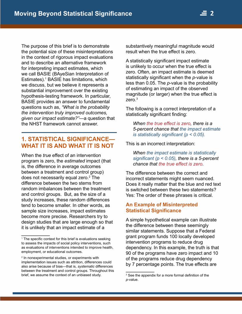
The purpose of this brief is to demonstrate the potential size of these misinterpretations in the context of rigorous impact evaluations and to describe an alternative framework for interpreting impact estimates which we call BASIE (BAyeSian Interpretation of Estimates)1 BASIE has limitations which we discuss but we believe it represents a substantial improvement over the existing hypothesis-testing framework In particular BASIE provides an answer to fundamental questions such as ldquoWhat is the probability the intervention truly improved outcomes given our impact estimaterdquomdasha question that the NHST framework cannot answer
1 STATISTICAL SIGNIFICANCEmdash WHAT IT IS AND WHAT IT IS NOT When the true effect of an intervention program is zero the estimated impact (that is the difference in average outcomes between a treatment and control group) does not necessarily equal zero2 The difference between the two stems from random imbalances between the treatment and control groups But as the size of a study increases these random differences tend to become smaller In other words as sample size increases impact estimates become more precise Researchers try to design studies that are large enough so that it is unlikely that an impact estimate of a
1 The specific context for this brief is evaluations seeking to assess the impacts of social policy interventions such as evaluations of interventions intended to improve health employment or educational outcomes 2 In nonexperimental studies or experiments with implementation issues such as attrition differences could also arise because of biasmdashthat is systematic differences between the treatment and control groups Throughout this brief we assume the context of an unbiased study
substantively meaningful magnitude would result when the true effect is zero
A statistically significant impact estimate is unlikely to occur when the true effect is zero Often an impact estimate is deemed statistically significant when the p-value is less than 005 The p-value is the probability of estimating an impact of the observed magnitude (or larger) when the true effect is zero3
The following is a correct interpretation of a statistically significant finding
When the true effect is zero there is a 5-percent chance that the impact estimate is statistically significant (p lt 005)
This is an incorrect interpretation
When the impact estimate is statistically significant (p lt 005) there is a 5-percent chance that the true effect is zero
The difference between the correct and incorrect statements might seem nuanced Does it really matter that the blue and red text is switched between these two statements Yes The order of these phrases is critical
An Example of Misinterpreted Statistical Significance
A simple hypothetical example can illustrate the difference between these seemingly similar statements Suppose that a Federal grant program funds 100 locally developed intervention programs to reduce drug dependency In this example the truth is that 90 of the programs have zero impact and 10 of the programs reduce drug dependency by 7 percentage points The true effects are
3 See the appendix for a more formal definition of the p-value
Moving Beyond Statistical Significance 3
unknown to policymakers or researchers Suppose we select one of these programs at random and evaluate it using a study that is big enough to have an 80-percent probability of detecting an impact of 7 percentage points (a fairly standard way to design a study) In this study we would declare an impact estimate statistically significant if the p-value was less than 005
This barrel contains four types of marbles
In this example we can calculate the probability that the true effect is zero when the impact estimate is statistically significant through a simple counting exercise that uses the information presented in the previous paragraph Figure 1 illustrates all the information presented in the previous paragraph represented as a barrel full of marbles In this barrel each marble represents the results from studying one program When the researcher randomly selects a program to study they are essentially reaching into this barrel and pulling out one of these marbles
Figure 1 A Barrel Full of Marbles Representing Potential Impact Studies
` Eight orange marbles represent studies in which the program is truly effective and the impact estimate is statistically significant The number of orange marbles is eight because we have 80 percent power to detect a true effect and there are 10 programs with true effects 08 times 10 = 8
` Two black marbles represent studies in which the program is truly effective but the impact estimate is not statistically significant If we expect to detect 80 percent of true effects that means we expect not to detect 20 percent of true effects 02 times 10 = 2
` Five purple marbles represent studies in which the program is not truly effective but the impact estimate is statistically significant The number of purple marbles is five because the probability of an impact estimate being statistically significant when the true effect is zero is 5 percent 005 times 90 = 45 (which we rounded up to 5)
` Eighty-five grey marbles represent studies in which the program is not truly effective and the impact estimate is not statistically significant If we expect 5 percent of ineffective interventions to have statistically significant impact estimates that means we expect 95 percent of ineffective interventions not to have statistically significant impact estimates 095 times 90 = 855 (which we round down to 85 so that all the marbles sum to 100)
The probability that the true effect is zero when the impact estimate is statistically significant can be calculated by counting
Moving Beyond Statistical Significance 4
marbles 5 purple marbles (5 purple marbles + 8 orange marbles) = about 38 percent
This example clearly illustrates that misinterpreting statistical significance is not a small mistake Although the probability that the impact estimate is statistically significant when the true effect is zero is just 5 percent (a probability that is typically calculated under the NHST framework) the probability that the true effect is zero when the impact estimate is statistically significant is approximately 38 percent (a probability that typically is not calculated under the NHST framework)
The Missing Link External Evidence
To assess the probability that an intervention is truly effective we must know what proportion of interventions are effective In the real world we do not know that with certainty In the example above we had that evidencemdashwe knew that only 10 percent of programs were effective With that evidence we could calculate the probability that the true effect was zero given our impact estimate (it was 38 percent) This calculation depended on a relationship involving conditional probabilities that was first described by an English minister named Thomas Bayes This relationship is called Bayesrsquo Rule4 The calculation 5 purple marbles (5 purple marbles + 8 orange marbles) is an example of the application of Bayesrsquo Rule
4 See the appendix for more detail on Bayesrsquo Rule including the equation
2 BASIE A HARD-HEADED INFERENTIAL FRAMEWORK FOR INTERPRETING FINDINGS FROM IMPACT EVALUATIONS In the world of high-stakes impact evaluations it is the job of policy makers to ask questions and the job of researchers to provide the most accurate answers possible These answers should be based on quantifiable verifiable evidence The answers should not be based on anyonersquos (not policymakersrsquo nor researchersrsquo) personal beliefs about the intervention being evaluated Although the NHST meets this criterion it does not answer the question policymakers most likely want to know
Hard-head-ed Adjective Practical and realistic not sentimental
Source Oxford English Dictionary
What is the probability that an intervention was effective given an observed impact Bayesian methods can answer this question but they often do so by drawing on prior beliefs regarding the effectiveness of the intervention being studied The advantage of BASIE is that it answers the question of interest to policymakers using quantifiable verifiable evidence BASIE is heavily influenced by researchers who have sought to use Bayesian methods for scientific purposes (Gelman 2011 Gelman amp Shalizi 2013 Gelman 2016) The components of BASIE are summarized in table 1 and discussed below
Probability With BASIE probability is based on things we can count Following the example of Gigerenzer and Hoffrage (1995) we think of probability in terms of relative
Moving Beyond Statistical Significance 5
frequencymdashthat is probability is defined in terms of tangible things that we can empirically count and model For example the probability of rolling an odd number on a six-sided die is 050 because there are three odd numbers six total numbers and 36 = 050 By way of comparison some Bayesian statisticians define probability in terms of the intensity of onersquos personal belief regarding the truth of a proposition (de Finetti 1974) We reject that subjective definition for this hard-headed framework
Priors Following Gelman (2015a) we draw on prior evidence (not prior belief) to develop an understanding of the probability that interventions have effects of various magnitudes For example we might look to an evidence review (such as the What Works Clearinghouse [WWC] or the Home Visiting Evidence of Effectiveness [HomVEE] reviews) for prior evidence on the distribution of intervention effects5 Combining our definition of probability as a relative frequency with our definition of priors as evidence based enables us to express prior probability using statements such as ldquoThe WWC reports impacts of 30 interventions designed to improve reading test scores for elementary school students Twenty-one of those 30 interventions had impacts of 015 standard deviations or higherrdquo In subsequent sections we discuss in more detail the selection of prior evidence the extent to which imperfect prior evidence can lead us astray and cases in which it might be appropriate to use modeling to combine or refine prior evidence When seeking to assess the probability that an intervention was effective we will see
5 For more information visit the WWC website (http iesedgovnceewwc) and the HomVEE website (http homveeacfhhsgov)
that it is generally better to use imperfect but thoughtfully selected prior evidence than to misinterpret a p-value and that increasing the sample size of a study will reduce sensitivity to prior evidence
Point estimates We recommend reporting both the traditional impact estimate based only on study data and an estimate incorporating prior evidence This second estimate is sometimes called a shrunken estimate because it essentially shrinks the traditional estimate toward the mean of the prior evidence Which estimate receives more emphasis will depend on how similar the new study is to the base of prior evidence and whether it is possible to make credible statistical adjustment for any important differences
Interpretation Although we recommend reporting point estimates that are not informed by prior evidence as well as point estimates that are we recommend always using prior evidence to interpret the impact estimate Using prior evidence is the only way to assess the probability that the intervention truly has a positive effect even if that prior evidence is substantively different from the new study (for example the new study might be focused on an outcome domain intervention model or implementation context that is not represented in the prior evidence)
Sensitivity analysis At multiple steps throughout a study researchers must choose from among different methodological approaches and it is important to assess the extent to which results vary across credible alternative approaches In the BASIE framework it is especially important to assess sensitivity to the choice of prior evidence We discuss sensitivity to priors in detail later in this brief
Moving Beyond Statistical Significance 6
Table 1 Components of the hard-headed BASIE framework for impact evaluation
Component Yes No Notes
Probability
A relative frequency (for example ldquo21 out of 30 relevant studies in HomVEErdquo)
Personal belief (for example ldquoI am 70 percent sure thathelliprdquo)
In this framework we can generally think of a probability as a number based on things that can be counted When communicating probabilities it is important to make sure we are clear about what is being counted
Prior Evidence Personal belief
We could combine or refine the prior evidence using a model but the fundamental basis of the prior is evidence not belief
Reported impact estimate
Both the impact estimated using only study data and the shrunken impact estimate incorporating prior evidence
Just the impact estimated using only study data or the shrunken impact estimate
The relevance of the prior evidence base to the current study will dictate which estimate we should highlight
Interpretation Bayesian posterior probabilities Bayesian credible intervals
Statistical significance p-values
As discussed in the text p-values and statistical significance are too easily misinterpreted and do not tell us what we really want to know the probability that the intervention truly improved outcomes We can appreciate that it might be necessary to report p-values and statistical significance because some stakeholders will continue to demand them but p-values and statistical significance are not a part of this framework
Sensitivity analysis
Reporting sensitivity of impact estimates and posterior probabilities to the selection and modeling of prior evidence
Reporting a single answer with no assessment of its robustness
Increasing the sample size of a study will reduce sensitivity to prior evidence
Source This framework is influenced by many sources including Gigerenzer and Hoffrage (1995) Gelman (2011) Gelman and Shalizi (2013) and the presentations and discussions at the Office of Planning Research and Evaluationrsquos 2017 Bayesian Methods for Social Policy Research and Evaluation meeting HomVEE = Home Visiting Evidence of Effectiveness
3 PLAUSIBLE PRIORS PRECEDE PERSUASIVE POSTERIORS As described previously estimating the probability that an intervention has a truly positive effect requires outside evidence about the proportion of interventions that have positive effects If similar interventions have rarely made large impacts on similar outcomes then we would infer that a very large impact of the current intervention is less likely By contrast the more common
Moving Beyond Statistical Significance 7
large effects have been in the past the more probable it is that a sizeable impact estimated using data from the current study is the result of a true effect rather than random chance This use of external information is what distinguishes Bayesian statistics from classical statistics
No to the flat prior At one time something called the flat prior was very popular The flat prior is centered at zero with infinite variance It was seen as objective because it assigns equal prior probability to all possible values of the impact impacts of 0 01 1 10 and 100 standard deviations are all treated as equally plausible The flat prior might seem reasonable when defining probability in terms of belief rather than evidencemdashone might imagine that the flat prior reflects the most impartial belief possible (Gelman et al 2013) As such this prior was de rigueur for decades falling out only recently But when we base probability on evidence the absurdity of the flat prior becomes apparent What evidence exists to support the notion that impacts of 0 01 1 10 and 100 standard deviations are all equally probable No such evidence exists and in fact quite a bit of evidence is completely inconsistent with this prior (for example the distribution of impact estimates in the WWC or the HomVEE review)6 Following Gelman and Weakliem (2009) we reject the flat prior because it has no basis in evidence
The flat prior and misinterpretation of p-values Bayesian flat-prior analysis is equivalent to misinterpreting the p-value because a Bayesian posterior probability derived under a flat prior is identical (at least for simple models) to a one-sided
6 For more information visit the HomVEE website (http homveeacfhhsgov) and the WWC website (httpies edgovnceewwc)
p-value Each time someone misinterprets a significant p-value as implying a high probability that the intervention truly works they are assuming a flat prior Therefore although Bayesian methods are often discussed as a possible solution to the reproducibility crisis in science Bayesian analyses that use a flat prior are no solution whatsoever If researchers switch to Bayesian methods but use a flat prior they will continue to exaggerate the probability of large program effects and continue to contribute to the reproducibility crisis
Yes to the evidence-based prior The evidence-based prior summarizes the impacts of a broader population of similar interventions In choosing the population we are deciding what prior evidence is relevant for the current evaluation For example the WWC is a rich source of prior evidence for education studies and the HomVEE review is a rich source of prior evidence for home visiting studies After we have chosen a relevant source of prior evidence we can calculate the prior probability of a meaningful impact by counting the relative frequency of meaningful impacts in the population such as ldquoThe WWC reports impacts of 30 interventions designed to improve reading test scores for elementary school students Twenty-one of those 30 interventions had impacts of 015 standard deviations or higherrdquo7
Challenges of specifying an evidence-based prior Choosing a population of relevant interventions is the key to specifying an evidence-based prior but determining how narrow or broad that
7 By meaningful impact we mean an impact of a magnitude deemed substantively important by relevant stakeholders or decision makers We are not referring to statistical significance
Moving Beyond Statistical Significance 8
population should be is often challenging In the previous example the prior comprised interventions that targeted elementary school students and focused on reading skills Would it have been better to make the population broader by including additional interventions focused on math skills or to make the population narrower by limiting the interventions to those that targeted only students in a specific grade Often a broad population might seem less relevant but it might be all that is available Furthermore narrower prior populations are at higher risk for cherry picking whereby researchers include favorable past studies in the prior with the goal of increasing the posterior probability that their current study produces meaningful impacts Lastly it is important not to completely rule out less likely but still plausible potential intervention effects For these three reasons the prior studies used to calculate probabilities should represent a wide but realistic range of possible intervention effects Sensitivity analyses can include narrower and broader priors
Two other challenges of specifying an evidence-based prior are that (a) evidence bases include impact estimates rather than true impacts and those estimates can be noisy and (b) prior evidence could be affected by publication bias or p-hacking (Gelman amp Loken 2014) In these cases it is appropriate to use modeling to combine or refine prior evidence For example noisy estimates can be down-weighted relative to more precise estimates and adjustments can be made for suspected biases
Given these challengesmdashas we will describe in more detail belowmdashit is crucial that evaluators (1) check how sensitive their inferences are to changing the prior and (2)
make it clear what information their prior is based on when they state their posterior
Consequences of using an imperfect evidence-based prior If we correctly specify the prior (and do everything else right) then our posterior probability statements will be correct too8 Specifically the posterior probability statements will be well calibrated meaning that if we made a number of probability statements at the 80-percent level (for example ldquoThere is an 80-percent chance that the intervention improves outcomesrdquo) and then went back after the fact and counted how many times the proposition in each statement turned out to be true the relative frequency of true statements would be 80 percent Unfortunately we can never perform this calibration in practice because we never ultimately observe the true impact of an intervention The best we can do is to use a simulation in which we do know the hypothetical truth to (1) verify that our methods produce well-calibrated probabilities when we correctly specify the prior and (2) assess the consequences of using imperfect prior evidence Such a simulation is described in the appendix The following are the key results
` Using a flat prior (or equivalently misinterpreting a p-value) leads us to overstate the probability of big effects (Gelman 2015b) This is because under the flat prior very large impacts are deemed just as likely as small impacts even when there is no evidence to support this For example under the flat prior the probabilities that an impact is greater than 005 and 5 standard
8 For the purpose of the discussion in this section we as-sume that there are no other problems with a studyrsquos design or data
Moving Beyond Statistical Significance 9
deviations are both about 50 percent9
By overstating the prior probability of big effects we also overstate the posterior probability of big effects
` Increasing the sample size of a study will reduce sensitivity to prior evidence
` An imperfect but thoughtfully selected evidence-based prior will generally lead to better posterior probabilities than the flat prior
4 SENSITIVITY ANALYSIS Given the challenges of specifying an evidence-based prior no single prior in and of itself might seem entirely credible Nonetheless evidence-based priors still boast important advantages over the flat prior which produces inferences that are equivalent to misinterpreting p-values as described previously We therefore recommend sensitivity analysis to determine how posterior probabilities vary across a plausible range of priors Findings that are robust across this range can be used with increased confidence to guide decision making For example the following candidate priors could be included in a sensitivity analysis
1 Take the literature at face value assuming no p-hacking or other selection biases
2 Assume that estimates in the literature are exaggerated by a factor of two on average
9 The probability that the impact is greater than 005 is infinitesimally larger than the probability that the true impact is greater than 5 standard deviations but both are about 50 percent This is attributable to the infinite variance of the flat prior
3 Account for possible overestimation of estimates in the literature more stringently by assuming that on average past impacts in this set of interventions equal zero
4 Include a broader or narrower population of prior studies
The results of such a sensitivity analysis provide bounds around posterior probability statements such as ldquoThe probability that the intervention improved outcomes by at least 02 standard deviations could be as low as 64 percent or as high as 91 percentrdquo
5 REPORTING IMPACT ESTIMATES When estimating the impact of a program under BASIE there are two point estimates that could be reported The first estimate is based on only study data not prior evidence This estimate is the traditional point estimate familiar to most researchers representing for example the difference in outcomes between the treatment and control groups The second estimate incorporates prior evidence into the estimate for the new study This shrunken estimate is a weighted average of the impact estimate using study data and the prior evidence The advantage of the shrunken estimator is that it is less susceptible to errors that arise from random baseline mismatches between a treatment and control group We recommend reporting both the traditional and shrunken estimates of a programrsquos impact
Exactly where each estimate is reported will depend on the situation Some studies might warrant a focus on the traditional estimates and other studies might best focus on the
Moving Beyond Statistical Significance 10
shrunken estimate The emphasis will depend on how similar the new study is to the base of prior evidence and whether it is possible to make credible statistical adjustment for any important differences In cases when a well-founded a priori expectation exists that the new intervention will have smaller or larger impacts than the interventions in the evidence base we recommend emphasizing the traditional estimate based on only study data (not the shrunken estimate) In cases in which the impacts from the evidence base are representative of what we expect from the new intervention we recommend emphasizing the shrunken impact estimate
For example consider an evaluation of a new program using a home visiting model that is much more resource intensive than anything previously evaluated We contend that it would be inappropriate to highlight the impact estimate informed by prior evidence in this case because we could reasonably expect the new high-intensity model to have larger impacts than the interventions in the evidence base In technical terms the impact estimate from the new study is not exchangeable with prior impact estimates in the evidence base By contrast in a replication study evaluating an intervention that already has a large evidence base the existing evidence base might be exchangeable with the impact estimate from the new study In this case it would be appropriate to highlight the estimate that incorporates external evidence to reduce the influence of random error in the impact estimate
Assessing the appropriateness of the exchangeability assumption is not always as easy as in the two extreme examples described previously In many cases reasonable arguments can be made in favor
of and against exchangeability For this reason we recommend reporting both even if one receives more emphasis
6 INTERPRETING POSTERIOR PROBABILITY STATEMENTS Although Bayesian posterior probabilities are easier to interpret than p-values and can more accurately assess the probability that an intervention works than can a misinterpreted p-value we do not mean to suggest that posterior probabilities are immune to misinterpretation These probabilities have a specific meaning and one can misinterpret posterior probabilities if they are not explained correctly and presented carefully In this section we discuss how to avoid these misinterpretations and we provide an example of how to correctly describe the posterior probability
Specifically there are three possible misinterpretations of Bayesian posterior probabilities that we think it important to guard against
1 Researchers might want to make a probability statement without doing the hard work of specifying an evidence-based prior ` Beware of glib probability statements
Recall that making a probability statement under a flat prior is equivalent to misinterpreting a p-value10
10 Another alternative is to use a prior that is not evidence based but is also not the flat prior Such a priormdashfor example the standard normal distributionmdashcan be appropriate for parameters that are not of substantive interest such as a residual variance parameter
Moving Beyond Statistical Significance 11
2 Readers of an impact study might want to know the probability that an intervention will work for them ` A Bayesian posterior probability
statement is relevant only to the population specified in the prior Therefore given that priors are typically broad posteriors must be as well
3 Readers might also want to make a predictive statement about the effect of an intervention in future contexts ` A posterior probability is a
retrospective statement regarding the impact of the evaluated intervention in the context it was evaluated For example the findings from a study conducted in the context of Chicago in 2010 might not apply in the context of Chicago in 2020 (Making predictive statements is possible but requires more modeling and assumptionsmdashit does not happen automatically)
The correct interpretation of a posterior probability cannot provide any of these things but it does still provide useful guidance as to which impact estimates deserve special attention Specifically a correctly interpreted posterior probability is an assessment of the probability that our intervention (the one we are studying) is truly effective given the findings of our study and the distribution of intervention effects (the prior distribution) in the population that we are assuming to be relevant It is crucial to be clear about what the population is when stating the posterior For example ldquoGiven the chances of having an impact greater than 015 standard deviations that we see
from past studies of reading programs for elementary school students combined with the impact estimate that we calculated in this study we estimate that there is a 75-percent probability that our intervention increased reading test scores by at least 015 standard deviations for the students included in this studyrdquo
7 PROBLEMS WITH IMPACT EVALUATIONS THAT BASIE CANNOT FIX BASIE addresses the problem of misinterpreting statistical significance but it does not address all the other reasons that evaluation findings can be inaccurate or misleading Evaluation findings can be inaccurate because of problems with an evaluationrsquos design analysis or data Evaluation findings can also be inaccurate or misleading for reasons that are more human than statistical Although the replication crisis in science might be attributable partly to an honest misinterpretation of statistical significance it might also be attributable to the bad incentives that arise when researchersrsquo professional success depends on the findings from a study rather than its quality For example the tendency for journal editors to publish only statistically significant results (publication bias) created the bad incentive for researchers to manipulate p-values (known as p-hacking) If journal editors continue to create bad incentives then researchers might find other ways to manipulate findings even under the BASIE framework BASIE represents an important improvement over the NHST framework but does not solve these other problems
Moving Beyond Statistical Significance 12
-
8 IN CONCLUSION A FRESH START We cannot continue to misinterpret p-values and statistical significance yet we also must provide decision makers with a credible assessment of the probability that an intervention actually worked In this brief we illustrated the potential magnitude of p-value misinterpretation and presented a framework that can serve to answer the important question What is the probability that an intervention worked
With BASIE evaluators will continue to provide answers to important policy questions based on evidencemdashnot anyonersquos personal beliefs But now we can provide those answers in a way that is more intuitive better aligned to questions of interest to decision makers and less susceptible to misinterpretation Although BASIE is not a panaceamdashthe answers it provides are not perfect and misinterpretations are still possiblemdashwe believe it represents a significant improvement over the hypothesis testing framework
This brief was prepared for the Office of Planning Research and Evaluation (OPRE) part of the US Department of Health and Human Servicesrsquo (HHS) Administration for Children and Families (ACF) It was developed under Contract Number HHSP233201500109I Insight Policy Research (Insight) located at 1901 North Moore Street Suite 1100 in Arlington Virginia assisted with preparing and formatting the brief The ACF project officer is Emily Ball Jabbour and the ACF project specialist is Kriti Jain The Insight project director is Rachel Holzwart and the Insight deputy project director is Hilary Wagner This brief is in the public domain Permission to reproduce is not necessary Suggested citation Deke J amp Finucane M (2019) Moving beyond statistical significance the BASIE (BAyeSian Interpretation of Estimates) Framework for interpreting findings from impact evaluations (OPRE Report 2019 35) Washington DC Office of Planning Research and Evaluation Administration for Children and Families US Department of Health and Human Services This brief and other reports sponsored by OPRE are available at wwwacfhhsgovopre Disclaimer The views expressed in this publication do not necessarily reflect the views or policies of OPRE ACF or HHS
Moving Beyond Statistical Significance 13
REFERENCES de Finetti B (1974) Theory of probability A critical introductory treatment New York NY
Wiley
Fisher R A (1925) Statistical methods for research workers Edinburgh Oliver and Boyd
Gelman A (2011) Induction and deduction in Bayesian data analysis Rationality Markets and Morals 2 67ndash78
Gelman A (2015a) Prior information not prior belief [Blog post] Retrieved from http andrewgelmancom20150715prior-information-not-prior-belief
Gelman A (2015b) The general problem I have with noninformatively-derived Bayesian probabilities is that they tend to be too strong [Blog post] Retrieved from http andrewgelmancom20150501general-problem-noninformatively-derived-bayesian-probabilities-tend-strong
Gelman A (2016) What is the lsquotrue prior distributionrsquo A hard-nosed answer [Blog post] Retrieved from httpandrewgelmancom20160423what-is-the-true-prior-distribution-a-hard-nosed-answer
Gelman A Carlin J B Stern H S Dunson D B Vehtari A amp Rubin D B (2013) Bayesian data analysis (3rd ed) Boca Raton FL CRC Press
Gelman A amp Loken E (2014) The statistical crisis in science American Scientist 102(6) 460
Gelman A amp Shalizi C (2013) Philosophy and the practice of Bayesian statistics British Journal of Mathematical and Statistical Psychology 66 8ndash38
Gelman A amp Weakliem D (2009) Of beauty sex and power American Scientist 97(4) 310ndash316
Gigerenzer G amp Hoffrage U (1995) How to improve Bayesian reasoning without instruction frequency formats Psychological Review 102 684ndash704
Greenland S Senn S J Rothman K J Carlin J B Poole C Goodman S N amp Altman D G (2016) Statistical tests p-values confidence intervals and power A guide to misinterpretations European Journal of Epidemiology 31(4) 337ndash350
McCloskey D N amp Ziliak S T (2008) The cult of statistical significance How the standard error costs us jobs justice and lives Ann Arbor MI University of Michigan Press
Neyman J amp Pearson E S (1933) On the problem of the most efficient tests of statistical hypotheses Philosophical Transactions of the Royal Society 231 289ndash337
Peng R (2015) The reproducibility crisis in science A statistical counterattack Significance 12(3) 30ndash32
Wasserstein R L amp Lazar N A (2016) The ASArsquos statement on p-values Context process and purpose The American Statistician 70(2) 129ndash133
Moving Beyond Statistical Significance 14
APPENDIX In this appendix we include equations and technical details of the simulation study We present these details in the same order as the topics appear in the brief
1 DEFINITION OF THE P-VALUE
(my_estimate)
The p-value is the probability of estimating an impact of the observed magnitude (or larger) conditional on the true effect being zero For a one-tailed test this probability is presented in equation 1 where p is the p-value is the impact estimator is the observed impact estimate and θ represents the true effect
[1] p = P( gt | θ = 0)(my_estimate)
2 CALCULATING BAYESIAN POSTERIOR PROBABILITIES Using Bayesrsquo Rule the posterior density function of a true parameter θ conditional on the data y is given by equation 2 where P is a probability density function In this equation the prior is P(θ) the likelihood is P(y|θ) and P(y) is a normalizing constant (which does not depend on θ) In the context of an experimental impact study the parameter of interest is the true effect and the data are summarized by the impact estimate and its standard error
[2]
3 SIMULATION STUDY OF THE CONSEQUENCES OF USING AN IMPERFECT PRIOR Given the challenges of specifying an evidence-based prior no single prior in and of itself might seem entirely credible This naturally raises the question What are the consequences of using an imperfect prior Because we never ultimately observe the true impact of an intervention it is not possible to answer this question using study data The best we can do is to use a simulation where we do know truth
In this simulation study we will assume that we know the true prior that is the true distribution of impacts in a population of similar interventions In each iteration of the simulation we will draw a true impact from that distribution simulate data given the drawn impact and then perform Bayesian inference assuming the wrong prior Summarizing across iterations of the simulation we will assess how our inferences are affected by using an imperfect prior
Methods
1 Assume that the true prior is N(01042 ) This distribution was chosen to correspond roughly with the empirical distribution of impact estimates in the WWC Under this prior the true proportion of interventions with an impact of 02 standard deviations or greater is about 40 percent
Moving Beyond Statistical Significance 15
bull bull bull
bull bull
bull 08 bull
bull
bull
bull
bull
2 For each iteration i of the simulation a Draw a true impact θi from the true prior distribution P(θ)equivN(01042 )
θi ~ P(θ)
b Simulate data yi from the likelihood P(yθ) given the drawn impact θi
yi ~ P(yθi)
c Perform Bayesian inference assuming the wrong normal prior P(θ)
P(θyi) prop P(yiθ) P(θ)
3 Averaging across iterations of the simulation calculate the average stated probability that the impact of the intervention is 02 standard deviations or greater For well-calibrated inferences this should be equal to the true value of 40 percent
Settings
We will consider all possible combinations of the following assumed prior parameters and sample sizes
` Assumed prior mean 0 01 (the truth) 02
` Assumed prior standard deviation 02 04 (the truth)
Infinity (This corresponds to a flat prior)
` Sample size assuming no clustering 10 100 1000 10000
Results
The results of the simulation are given in figure 2 The following are the key findings
` When our assumed prior is correct our posterior probability statements are well calibrated meaning that on average we report the correct probability (40 percent) that an
Moving Beyond Statistical Significance 16
interventionrsquos impact is 02 standard deviations or greater This result which is depicted as a green line in the middle panel of the figure holds for all sample sizes
` The adverse consequences of using any imperfect prior diminish as sample size increases Specifically when n = 10000 (see the right side of each panel of the figure) on average we report approximately the correct probability that an interventionrsquos impact is 02 standard deviations or greater (40 percent) regardless of which prior we assume
` Using a flat prior (or equivalently misinterpreting a p-value) leads us to overstate the probability that an interventionrsquos impact is 02 standard deviations or greater This anticonservative bias which is depicted as a purple line in each panel of the figure diminishes as sample size increases
` It is generally better to use imperfect but thoughtfully selected prior evidence than a flat prior (or equivalently to misinterpret a p-value) See for example the blue lines in each of the first two panelsmdashthey show that as long as you do not overestimate the prior mean nor underestimate the prior standard deviation your posterior probability statements will be more accurate than those derived under a flat prior
Figure 2 Simulation Results on the Consequences of Using an Imperfect Prior
Note The true prior is N(01 042) SD = standard deviation
Sign-up for the ACF Like OPRE on Facebook Follow OPRE on Twitter OPRE News E-Newsletter FacebookcomOPREACF OPRE_ACF
Moving Beyond Statistical Significance 2
The purpose of this brief is to demonstrate the potential size of these misinterpretations in the context of rigorous impact evaluations and to describe an alternative framework for interpreting impact estimates which we call BASIE (BAyeSian Interpretation of Estimates)1 BASIE has limitations which we discuss but we believe it represents a substantial improvement over the existing hypothesis-testing framework In particular BASIE provides an answer to fundamental questions such as ldquoWhat is the probability the intervention truly improved outcomes given our impact estimaterdquomdasha question that the NHST framework cannot answer
1 STATISTICAL SIGNIFICANCEmdash WHAT IT IS AND WHAT IT IS NOT When the true effect of an intervention program is zero the estimated impact (that is the difference in average outcomes between a treatment and control group) does not necessarily equal zero2 The difference between the two stems from random imbalances between the treatment and control groups But as the size of a study increases these random differences tend to become smaller In other words as sample size increases impact estimates become more precise Researchers try to design studies that are large enough so that it is unlikely that an impact estimate of a
1 The specific context for this brief is evaluations seeking to assess the impacts of social policy interventions such as evaluations of interventions intended to improve health employment or educational outcomes 2 In nonexperimental studies or experiments with implementation issues such as attrition differences could also arise because of biasmdashthat is systematic differences between the treatment and control groups Throughout this brief we assume the context of an unbiased study
substantively meaningful magnitude would result when the true effect is zero
A statistically significant impact estimate is unlikely to occur when the true effect is zero Often an impact estimate is deemed statistically significant when the p-value is less than 005 The p-value is the probability of estimating an impact of the observed magnitude (or larger) when the true effect is zero3
The following is a correct interpretation of a statistically significant finding
When the true effect is zero there is a 5-percent chance that the impact estimate is statistically significant (p lt 005)
This is an incorrect interpretation
When the impact estimate is statistically significant (p lt 005) there is a 5-percent chance that the true effect is zero
The difference between the correct and incorrect statements might seem nuanced Does it really matter that the blue and red text is switched between these two statements Yes The order of these phrases is critical
An Example of Misinterpreted Statistical Significance
A simple hypothetical example can illustrate the difference between these seemingly similar statements Suppose that a Federal grant program funds 100 locally developed intervention programs to reduce drug dependency In this example the truth is that 90 of the programs have zero impact and 10 of the programs reduce drug dependency by 7 percentage points The true effects are
3 See the appendix for a more formal definition of the p-value
Moving Beyond Statistical Significance 3
unknown to policymakers or researchers Suppose we select one of these programs at random and evaluate it using a study that is big enough to have an 80-percent probability of detecting an impact of 7 percentage points (a fairly standard way to design a study) In this study we would declare an impact estimate statistically significant if the p-value was less than 005
This barrel contains four types of marbles
In this example we can calculate the probability that the true effect is zero when the impact estimate is statistically significant through a simple counting exercise that uses the information presented in the previous paragraph Figure 1 illustrates all the information presented in the previous paragraph represented as a barrel full of marbles In this barrel each marble represents the results from studying one program When the researcher randomly selects a program to study they are essentially reaching into this barrel and pulling out one of these marbles
Figure 1 A Barrel Full of Marbles Representing Potential Impact Studies
` Eight orange marbles represent studies in which the program is truly effective and the impact estimate is statistically significant The number of orange marbles is eight because we have 80 percent power to detect a true effect and there are 10 programs with true effects 08 times 10 = 8
` Two black marbles represent studies in which the program is truly effective but the impact estimate is not statistically significant If we expect to detect 80 percent of true effects that means we expect not to detect 20 percent of true effects 02 times 10 = 2
` Five purple marbles represent studies in which the program is not truly effective but the impact estimate is statistically significant The number of purple marbles is five because the probability of an impact estimate being statistically significant when the true effect is zero is 5 percent 005 times 90 = 45 (which we rounded up to 5)
` Eighty-five grey marbles represent studies in which the program is not truly effective and the impact estimate is not statistically significant If we expect 5 percent of ineffective interventions to have statistically significant impact estimates that means we expect 95 percent of ineffective interventions not to have statistically significant impact estimates 095 times 90 = 855 (which we round down to 85 so that all the marbles sum to 100)
The probability that the true effect is zero when the impact estimate is statistically significant can be calculated by counting
Moving Beyond Statistical Significance 4
marbles 5 purple marbles (5 purple marbles + 8 orange marbles) = about 38 percent
This example clearly illustrates that misinterpreting statistical significance is not a small mistake Although the probability that the impact estimate is statistically significant when the true effect is zero is just 5 percent (a probability that is typically calculated under the NHST framework) the probability that the true effect is zero when the impact estimate is statistically significant is approximately 38 percent (a probability that typically is not calculated under the NHST framework)
The Missing Link External Evidence
To assess the probability that an intervention is truly effective we must know what proportion of interventions are effective In the real world we do not know that with certainty In the example above we had that evidencemdashwe knew that only 10 percent of programs were effective With that evidence we could calculate the probability that the true effect was zero given our impact estimate (it was 38 percent) This calculation depended on a relationship involving conditional probabilities that was first described by an English minister named Thomas Bayes This relationship is called Bayesrsquo Rule4 The calculation 5 purple marbles (5 purple marbles + 8 orange marbles) is an example of the application of Bayesrsquo Rule
4 See the appendix for more detail on Bayesrsquo Rule including the equation
2 BASIE A HARD-HEADED INFERENTIAL FRAMEWORK FOR INTERPRETING FINDINGS FROM IMPACT EVALUATIONS In the world of high-stakes impact evaluations it is the job of policy makers to ask questions and the job of researchers to provide the most accurate answers possible These answers should be based on quantifiable verifiable evidence The answers should not be based on anyonersquos (not policymakersrsquo nor researchersrsquo) personal beliefs about the intervention being evaluated Although the NHST meets this criterion it does not answer the question policymakers most likely want to know
Hard-head-ed Adjective Practical and realistic not sentimental
Source Oxford English Dictionary
What is the probability that an intervention was effective given an observed impact Bayesian methods can answer this question but they often do so by drawing on prior beliefs regarding the effectiveness of the intervention being studied The advantage of BASIE is that it answers the question of interest to policymakers using quantifiable verifiable evidence BASIE is heavily influenced by researchers who have sought to use Bayesian methods for scientific purposes (Gelman 2011 Gelman amp Shalizi 2013 Gelman 2016) The components of BASIE are summarized in table 1 and discussed below
Probability With BASIE probability is based on things we can count Following the example of Gigerenzer and Hoffrage (1995) we think of probability in terms of relative
Moving Beyond Statistical Significance 5
frequencymdashthat is probability is defined in terms of tangible things that we can empirically count and model For example the probability of rolling an odd number on a six-sided die is 050 because there are three odd numbers six total numbers and 36 = 050 By way of comparison some Bayesian statisticians define probability in terms of the intensity of onersquos personal belief regarding the truth of a proposition (de Finetti 1974) We reject that subjective definition for this hard-headed framework
Priors Following Gelman (2015a) we draw on prior evidence (not prior belief) to develop an understanding of the probability that interventions have effects of various magnitudes For example we might look to an evidence review (such as the What Works Clearinghouse [WWC] or the Home Visiting Evidence of Effectiveness [HomVEE] reviews) for prior evidence on the distribution of intervention effects5 Combining our definition of probability as a relative frequency with our definition of priors as evidence based enables us to express prior probability using statements such as ldquoThe WWC reports impacts of 30 interventions designed to improve reading test scores for elementary school students Twenty-one of those 30 interventions had impacts of 015 standard deviations or higherrdquo In subsequent sections we discuss in more detail the selection of prior evidence the extent to which imperfect prior evidence can lead us astray and cases in which it might be appropriate to use modeling to combine or refine prior evidence When seeking to assess the probability that an intervention was effective we will see
5 For more information visit the WWC website (http iesedgovnceewwc) and the HomVEE website (http homveeacfhhsgov)
that it is generally better to use imperfect but thoughtfully selected prior evidence than to misinterpret a p-value and that increasing the sample size of a study will reduce sensitivity to prior evidence
Point estimates We recommend reporting both the traditional impact estimate based only on study data and an estimate incorporating prior evidence This second estimate is sometimes called a shrunken estimate because it essentially shrinks the traditional estimate toward the mean of the prior evidence Which estimate receives more emphasis will depend on how similar the new study is to the base of prior evidence and whether it is possible to make credible statistical adjustment for any important differences
Interpretation Although we recommend reporting point estimates that are not informed by prior evidence as well as point estimates that are we recommend always using prior evidence to interpret the impact estimate Using prior evidence is the only way to assess the probability that the intervention truly has a positive effect even if that prior evidence is substantively different from the new study (for example the new study might be focused on an outcome domain intervention model or implementation context that is not represented in the prior evidence)
Sensitivity analysis At multiple steps throughout a study researchers must choose from among different methodological approaches and it is important to assess the extent to which results vary across credible alternative approaches In the BASIE framework it is especially important to assess sensitivity to the choice of prior evidence We discuss sensitivity to priors in detail later in this brief
Moving Beyond Statistical Significance 6
Table 1 Components of the hard-headed BASIE framework for impact evaluation
Component Yes No Notes
Probability
A relative frequency (for example ldquo21 out of 30 relevant studies in HomVEErdquo)
Personal belief (for example ldquoI am 70 percent sure thathelliprdquo)
In this framework we can generally think of a probability as a number based on things that can be counted When communicating probabilities it is important to make sure we are clear about what is being counted
Prior Evidence Personal belief
We could combine or refine the prior evidence using a model but the fundamental basis of the prior is evidence not belief
Reported impact estimate
Both the impact estimated using only study data and the shrunken impact estimate incorporating prior evidence
Just the impact estimated using only study data or the shrunken impact estimate
The relevance of the prior evidence base to the current study will dictate which estimate we should highlight
Interpretation Bayesian posterior probabilities Bayesian credible intervals
Statistical significance p-values
As discussed in the text p-values and statistical significance are too easily misinterpreted and do not tell us what we really want to know the probability that the intervention truly improved outcomes We can appreciate that it might be necessary to report p-values and statistical significance because some stakeholders will continue to demand them but p-values and statistical significance are not a part of this framework
Sensitivity analysis
Reporting sensitivity of impact estimates and posterior probabilities to the selection and modeling of prior evidence
Reporting a single answer with no assessment of its robustness
Increasing the sample size of a study will reduce sensitivity to prior evidence
Source This framework is influenced by many sources including Gigerenzer and Hoffrage (1995) Gelman (2011) Gelman and Shalizi (2013) and the presentations and discussions at the Office of Planning Research and Evaluationrsquos 2017 Bayesian Methods for Social Policy Research and Evaluation meeting HomVEE = Home Visiting Evidence of Effectiveness
3 PLAUSIBLE PRIORS PRECEDE PERSUASIVE POSTERIORS As described previously estimating the probability that an intervention has a truly positive effect requires outside evidence about the proportion of interventions that have positive effects If similar interventions have rarely made large impacts on similar outcomes then we would infer that a very large impact of the current intervention is less likely By contrast the more common
Moving Beyond Statistical Significance 7
large effects have been in the past the more probable it is that a sizeable impact estimated using data from the current study is the result of a true effect rather than random chance This use of external information is what distinguishes Bayesian statistics from classical statistics
No to the flat prior At one time something called the flat prior was very popular The flat prior is centered at zero with infinite variance It was seen as objective because it assigns equal prior probability to all possible values of the impact impacts of 0 01 1 10 and 100 standard deviations are all treated as equally plausible The flat prior might seem reasonable when defining probability in terms of belief rather than evidencemdashone might imagine that the flat prior reflects the most impartial belief possible (Gelman et al 2013) As such this prior was de rigueur for decades falling out only recently But when we base probability on evidence the absurdity of the flat prior becomes apparent What evidence exists to support the notion that impacts of 0 01 1 10 and 100 standard deviations are all equally probable No such evidence exists and in fact quite a bit of evidence is completely inconsistent with this prior (for example the distribution of impact estimates in the WWC or the HomVEE review)6 Following Gelman and Weakliem (2009) we reject the flat prior because it has no basis in evidence
The flat prior and misinterpretation of p-values Bayesian flat-prior analysis is equivalent to misinterpreting the p-value because a Bayesian posterior probability derived under a flat prior is identical (at least for simple models) to a one-sided
6 For more information visit the HomVEE website (http homveeacfhhsgov) and the WWC website (httpies edgovnceewwc)
p-value Each time someone misinterprets a significant p-value as implying a high probability that the intervention truly works they are assuming a flat prior Therefore although Bayesian methods are often discussed as a possible solution to the reproducibility crisis in science Bayesian analyses that use a flat prior are no solution whatsoever If researchers switch to Bayesian methods but use a flat prior they will continue to exaggerate the probability of large program effects and continue to contribute to the reproducibility crisis
Yes to the evidence-based prior The evidence-based prior summarizes the impacts of a broader population of similar interventions In choosing the population we are deciding what prior evidence is relevant for the current evaluation For example the WWC is a rich source of prior evidence for education studies and the HomVEE review is a rich source of prior evidence for home visiting studies After we have chosen a relevant source of prior evidence we can calculate the prior probability of a meaningful impact by counting the relative frequency of meaningful impacts in the population such as ldquoThe WWC reports impacts of 30 interventions designed to improve reading test scores for elementary school students Twenty-one of those 30 interventions had impacts of 015 standard deviations or higherrdquo7
Challenges of specifying an evidence-based prior Choosing a population of relevant interventions is the key to specifying an evidence-based prior but determining how narrow or broad that
7 By meaningful impact we mean an impact of a magnitude deemed substantively important by relevant stakeholders or decision makers We are not referring to statistical significance
Moving Beyond Statistical Significance 8
population should be is often challenging In the previous example the prior comprised interventions that targeted elementary school students and focused on reading skills Would it have been better to make the population broader by including additional interventions focused on math skills or to make the population narrower by limiting the interventions to those that targeted only students in a specific grade Often a broad population might seem less relevant but it might be all that is available Furthermore narrower prior populations are at higher risk for cherry picking whereby researchers include favorable past studies in the prior with the goal of increasing the posterior probability that their current study produces meaningful impacts Lastly it is important not to completely rule out less likely but still plausible potential intervention effects For these three reasons the prior studies used to calculate probabilities should represent a wide but realistic range of possible intervention effects Sensitivity analyses can include narrower and broader priors
Two other challenges of specifying an evidence-based prior are that (a) evidence bases include impact estimates rather than true impacts and those estimates can be noisy and (b) prior evidence could be affected by publication bias or p-hacking (Gelman amp Loken 2014) In these cases it is appropriate to use modeling to combine or refine prior evidence For example noisy estimates can be down-weighted relative to more precise estimates and adjustments can be made for suspected biases
Given these challengesmdashas we will describe in more detail belowmdashit is crucial that evaluators (1) check how sensitive their inferences are to changing the prior and (2)
make it clear what information their prior is based on when they state their posterior
Consequences of using an imperfect evidence-based prior If we correctly specify the prior (and do everything else right) then our posterior probability statements will be correct too8 Specifically the posterior probability statements will be well calibrated meaning that if we made a number of probability statements at the 80-percent level (for example ldquoThere is an 80-percent chance that the intervention improves outcomesrdquo) and then went back after the fact and counted how many times the proposition in each statement turned out to be true the relative frequency of true statements would be 80 percent Unfortunately we can never perform this calibration in practice because we never ultimately observe the true impact of an intervention The best we can do is to use a simulation in which we do know the hypothetical truth to (1) verify that our methods produce well-calibrated probabilities when we correctly specify the prior and (2) assess the consequences of using imperfect prior evidence Such a simulation is described in the appendix The following are the key results
` Using a flat prior (or equivalently misinterpreting a p-value) leads us to overstate the probability of big effects (Gelman 2015b) This is because under the flat prior very large impacts are deemed just as likely as small impacts even when there is no evidence to support this For example under the flat prior the probabilities that an impact is greater than 005 and 5 standard
8 For the purpose of the discussion in this section we as-sume that there are no other problems with a studyrsquos design or data
Moving Beyond Statistical Significance 9
deviations are both about 50 percent9
By overstating the prior probability of big effects we also overstate the posterior probability of big effects
` Increasing the sample size of a study will reduce sensitivity to prior evidence
` An imperfect but thoughtfully selected evidence-based prior will generally lead to better posterior probabilities than the flat prior
4 SENSITIVITY ANALYSIS Given the challenges of specifying an evidence-based prior no single prior in and of itself might seem entirely credible Nonetheless evidence-based priors still boast important advantages over the flat prior which produces inferences that are equivalent to misinterpreting p-values as described previously We therefore recommend sensitivity analysis to determine how posterior probabilities vary across a plausible range of priors Findings that are robust across this range can be used with increased confidence to guide decision making For example the following candidate priors could be included in a sensitivity analysis
1 Take the literature at face value assuming no p-hacking or other selection biases
2 Assume that estimates in the literature are exaggerated by a factor of two on average
9 The probability that the impact is greater than 005 is infinitesimally larger than the probability that the true impact is greater than 5 standard deviations but both are about 50 percent This is attributable to the infinite variance of the flat prior
3 Account for possible overestimation of estimates in the literature more stringently by assuming that on average past impacts in this set of interventions equal zero
4 Include a broader or narrower population of prior studies
The results of such a sensitivity analysis provide bounds around posterior probability statements such as ldquoThe probability that the intervention improved outcomes by at least 02 standard deviations could be as low as 64 percent or as high as 91 percentrdquo
5 REPORTING IMPACT ESTIMATES When estimating the impact of a program under BASIE there are two point estimates that could be reported The first estimate is based on only study data not prior evidence This estimate is the traditional point estimate familiar to most researchers representing for example the difference in outcomes between the treatment and control groups The second estimate incorporates prior evidence into the estimate for the new study This shrunken estimate is a weighted average of the impact estimate using study data and the prior evidence The advantage of the shrunken estimator is that it is less susceptible to errors that arise from random baseline mismatches between a treatment and control group We recommend reporting both the traditional and shrunken estimates of a programrsquos impact
Exactly where each estimate is reported will depend on the situation Some studies might warrant a focus on the traditional estimates and other studies might best focus on the
Moving Beyond Statistical Significance 10
shrunken estimate The emphasis will depend on how similar the new study is to the base of prior evidence and whether it is possible to make credible statistical adjustment for any important differences In cases when a well-founded a priori expectation exists that the new intervention will have smaller or larger impacts than the interventions in the evidence base we recommend emphasizing the traditional estimate based on only study data (not the shrunken estimate) In cases in which the impacts from the evidence base are representative of what we expect from the new intervention we recommend emphasizing the shrunken impact estimate
For example consider an evaluation of a new program using a home visiting model that is much more resource intensive than anything previously evaluated We contend that it would be inappropriate to highlight the impact estimate informed by prior evidence in this case because we could reasonably expect the new high-intensity model to have larger impacts than the interventions in the evidence base In technical terms the impact estimate from the new study is not exchangeable with prior impact estimates in the evidence base By contrast in a replication study evaluating an intervention that already has a large evidence base the existing evidence base might be exchangeable with the impact estimate from the new study In this case it would be appropriate to highlight the estimate that incorporates external evidence to reduce the influence of random error in the impact estimate
Assessing the appropriateness of the exchangeability assumption is not always as easy as in the two extreme examples described previously In many cases reasonable arguments can be made in favor
of and against exchangeability For this reason we recommend reporting both even if one receives more emphasis
6 INTERPRETING POSTERIOR PROBABILITY STATEMENTS Although Bayesian posterior probabilities are easier to interpret than p-values and can more accurately assess the probability that an intervention works than can a misinterpreted p-value we do not mean to suggest that posterior probabilities are immune to misinterpretation These probabilities have a specific meaning and one can misinterpret posterior probabilities if they are not explained correctly and presented carefully In this section we discuss how to avoid these misinterpretations and we provide an example of how to correctly describe the posterior probability
Specifically there are three possible misinterpretations of Bayesian posterior probabilities that we think it important to guard against
1 Researchers might want to make a probability statement without doing the hard work of specifying an evidence-based prior ` Beware of glib probability statements
Recall that making a probability statement under a flat prior is equivalent to misinterpreting a p-value10
10 Another alternative is to use a prior that is not evidence based but is also not the flat prior Such a priormdashfor example the standard normal distributionmdashcan be appropriate for parameters that are not of substantive interest such as a residual variance parameter
Moving Beyond Statistical Significance 11
2 Readers of an impact study might want to know the probability that an intervention will work for them ` A Bayesian posterior probability
statement is relevant only to the population specified in the prior Therefore given that priors are typically broad posteriors must be as well
3 Readers might also want to make a predictive statement about the effect of an intervention in future contexts ` A posterior probability is a
retrospective statement regarding the impact of the evaluated intervention in the context it was evaluated For example the findings from a study conducted in the context of Chicago in 2010 might not apply in the context of Chicago in 2020 (Making predictive statements is possible but requires more modeling and assumptionsmdashit does not happen automatically)
The correct interpretation of a posterior probability cannot provide any of these things but it does still provide useful guidance as to which impact estimates deserve special attention Specifically a correctly interpreted posterior probability is an assessment of the probability that our intervention (the one we are studying) is truly effective given the findings of our study and the distribution of intervention effects (the prior distribution) in the population that we are assuming to be relevant It is crucial to be clear about what the population is when stating the posterior For example ldquoGiven the chances of having an impact greater than 015 standard deviations that we see
from past studies of reading programs for elementary school students combined with the impact estimate that we calculated in this study we estimate that there is a 75-percent probability that our intervention increased reading test scores by at least 015 standard deviations for the students included in this studyrdquo
7 PROBLEMS WITH IMPACT EVALUATIONS THAT BASIE CANNOT FIX BASIE addresses the problem of misinterpreting statistical significance but it does not address all the other reasons that evaluation findings can be inaccurate or misleading Evaluation findings can be inaccurate because of problems with an evaluationrsquos design analysis or data Evaluation findings can also be inaccurate or misleading for reasons that are more human than statistical Although the replication crisis in science might be attributable partly to an honest misinterpretation of statistical significance it might also be attributable to the bad incentives that arise when researchersrsquo professional success depends on the findings from a study rather than its quality For example the tendency for journal editors to publish only statistically significant results (publication bias) created the bad incentive for researchers to manipulate p-values (known as p-hacking) If journal editors continue to create bad incentives then researchers might find other ways to manipulate findings even under the BASIE framework BASIE represents an important improvement over the NHST framework but does not solve these other problems
Moving Beyond Statistical Significance 12
-
8 IN CONCLUSION A FRESH START We cannot continue to misinterpret p-values and statistical significance yet we also must provide decision makers with a credible assessment of the probability that an intervention actually worked In this brief we illustrated the potential magnitude of p-value misinterpretation and presented a framework that can serve to answer the important question What is the probability that an intervention worked
With BASIE evaluators will continue to provide answers to important policy questions based on evidencemdashnot anyonersquos personal beliefs But now we can provide those answers in a way that is more intuitive better aligned to questions of interest to decision makers and less susceptible to misinterpretation Although BASIE is not a panaceamdashthe answers it provides are not perfect and misinterpretations are still possiblemdashwe believe it represents a significant improvement over the hypothesis testing framework
This brief was prepared for the Office of Planning Research and Evaluation (OPRE) part of the US Department of Health and Human Servicesrsquo (HHS) Administration for Children and Families (ACF) It was developed under Contract Number HHSP233201500109I Insight Policy Research (Insight) located at 1901 North Moore Street Suite 1100 in Arlington Virginia assisted with preparing and formatting the brief The ACF project officer is Emily Ball Jabbour and the ACF project specialist is Kriti Jain The Insight project director is Rachel Holzwart and the Insight deputy project director is Hilary Wagner This brief is in the public domain Permission to reproduce is not necessary Suggested citation Deke J amp Finucane M (2019) Moving beyond statistical significance the BASIE (BAyeSian Interpretation of Estimates) Framework for interpreting findings from impact evaluations (OPRE Report 2019 35) Washington DC Office of Planning Research and Evaluation Administration for Children and Families US Department of Health and Human Services This brief and other reports sponsored by OPRE are available at wwwacfhhsgovopre Disclaimer The views expressed in this publication do not necessarily reflect the views or policies of OPRE ACF or HHS
Moving Beyond Statistical Significance 13
REFERENCES de Finetti B (1974) Theory of probability A critical introductory treatment New York NY
Wiley
Fisher R A (1925) Statistical methods for research workers Edinburgh Oliver and Boyd
Gelman A (2011) Induction and deduction in Bayesian data analysis Rationality Markets and Morals 2 67ndash78
Gelman A (2015a) Prior information not prior belief [Blog post] Retrieved from http andrewgelmancom20150715prior-information-not-prior-belief
Gelman A (2015b) The general problem I have with noninformatively-derived Bayesian probabilities is that they tend to be too strong [Blog post] Retrieved from http andrewgelmancom20150501general-problem-noninformatively-derived-bayesian-probabilities-tend-strong
Gelman A (2016) What is the lsquotrue prior distributionrsquo A hard-nosed answer [Blog post] Retrieved from httpandrewgelmancom20160423what-is-the-true-prior-distribution-a-hard-nosed-answer
Gelman A Carlin J B Stern H S Dunson D B Vehtari A amp Rubin D B (2013) Bayesian data analysis (3rd ed) Boca Raton FL CRC Press
Gelman A amp Loken E (2014) The statistical crisis in science American Scientist 102(6) 460
Gelman A amp Shalizi C (2013) Philosophy and the practice of Bayesian statistics British Journal of Mathematical and Statistical Psychology 66 8ndash38
Gelman A amp Weakliem D (2009) Of beauty sex and power American Scientist 97(4) 310ndash316
Gigerenzer G amp Hoffrage U (1995) How to improve Bayesian reasoning without instruction frequency formats Psychological Review 102 684ndash704
Greenland S Senn S J Rothman K J Carlin J B Poole C Goodman S N amp Altman D G (2016) Statistical tests p-values confidence intervals and power A guide to misinterpretations European Journal of Epidemiology 31(4) 337ndash350
McCloskey D N amp Ziliak S T (2008) The cult of statistical significance How the standard error costs us jobs justice and lives Ann Arbor MI University of Michigan Press
Neyman J amp Pearson E S (1933) On the problem of the most efficient tests of statistical hypotheses Philosophical Transactions of the Royal Society 231 289ndash337
Peng R (2015) The reproducibility crisis in science A statistical counterattack Significance 12(3) 30ndash32
Wasserstein R L amp Lazar N A (2016) The ASArsquos statement on p-values Context process and purpose The American Statistician 70(2) 129ndash133
Moving Beyond Statistical Significance 14
APPENDIX In this appendix we include equations and technical details of the simulation study We present these details in the same order as the topics appear in the brief
1 DEFINITION OF THE P-VALUE
(my_estimate)
The p-value is the probability of estimating an impact of the observed magnitude (or larger) conditional on the true effect being zero For a one-tailed test this probability is presented in equation 1 where p is the p-value is the impact estimator is the observed impact estimate and θ represents the true effect
[1] p = P( gt | θ = 0)(my_estimate)
2 CALCULATING BAYESIAN POSTERIOR PROBABILITIES Using Bayesrsquo Rule the posterior density function of a true parameter θ conditional on the data y is given by equation 2 where P is a probability density function In this equation the prior is P(θ) the likelihood is P(y|θ) and P(y) is a normalizing constant (which does not depend on θ) In the context of an experimental impact study the parameter of interest is the true effect and the data are summarized by the impact estimate and its standard error
[2]
3 SIMULATION STUDY OF THE CONSEQUENCES OF USING AN IMPERFECT PRIOR Given the challenges of specifying an evidence-based prior no single prior in and of itself might seem entirely credible This naturally raises the question What are the consequences of using an imperfect prior Because we never ultimately observe the true impact of an intervention it is not possible to answer this question using study data The best we can do is to use a simulation where we do know truth
In this simulation study we will assume that we know the true prior that is the true distribution of impacts in a population of similar interventions In each iteration of the simulation we will draw a true impact from that distribution simulate data given the drawn impact and then perform Bayesian inference assuming the wrong prior Summarizing across iterations of the simulation we will assess how our inferences are affected by using an imperfect prior
Methods
1 Assume that the true prior is N(01042 ) This distribution was chosen to correspond roughly with the empirical distribution of impact estimates in the WWC Under this prior the true proportion of interventions with an impact of 02 standard deviations or greater is about 40 percent
Moving Beyond Statistical Significance 15
bull bull bull
bull bull
bull 08 bull
bull
bull
bull
bull
2 For each iteration i of the simulation a Draw a true impact θi from the true prior distribution P(θ)equivN(01042 )
θi ~ P(θ)
b Simulate data yi from the likelihood P(yθ) given the drawn impact θi
yi ~ P(yθi)
c Perform Bayesian inference assuming the wrong normal prior P(θ)
P(θyi) prop P(yiθ) P(θ)
3 Averaging across iterations of the simulation calculate the average stated probability that the impact of the intervention is 02 standard deviations or greater For well-calibrated inferences this should be equal to the true value of 40 percent
Settings
We will consider all possible combinations of the following assumed prior parameters and sample sizes
` Assumed prior mean 0 01 (the truth) 02
` Assumed prior standard deviation 02 04 (the truth)
Infinity (This corresponds to a flat prior)
` Sample size assuming no clustering 10 100 1000 10000
Results
The results of the simulation are given in figure 2 The following are the key findings
` When our assumed prior is correct our posterior probability statements are well calibrated meaning that on average we report the correct probability (40 percent) that an
Moving Beyond Statistical Significance 16
interventionrsquos impact is 02 standard deviations or greater This result which is depicted as a green line in the middle panel of the figure holds for all sample sizes
` The adverse consequences of using any imperfect prior diminish as sample size increases Specifically when n = 10000 (see the right side of each panel of the figure) on average we report approximately the correct probability that an interventionrsquos impact is 02 standard deviations or greater (40 percent) regardless of which prior we assume
` Using a flat prior (or equivalently misinterpreting a p-value) leads us to overstate the probability that an interventionrsquos impact is 02 standard deviations or greater This anticonservative bias which is depicted as a purple line in each panel of the figure diminishes as sample size increases
` It is generally better to use imperfect but thoughtfully selected prior evidence than a flat prior (or equivalently to misinterpret a p-value) See for example the blue lines in each of the first two panelsmdashthey show that as long as you do not overestimate the prior mean nor underestimate the prior standard deviation your posterior probability statements will be more accurate than those derived under a flat prior
Figure 2 Simulation Results on the Consequences of Using an Imperfect Prior
Note The true prior is N(01 042) SD = standard deviation
Sign-up for the ACF Like OPRE on Facebook Follow OPRE on Twitter OPRE News E-Newsletter FacebookcomOPREACF OPRE_ACF
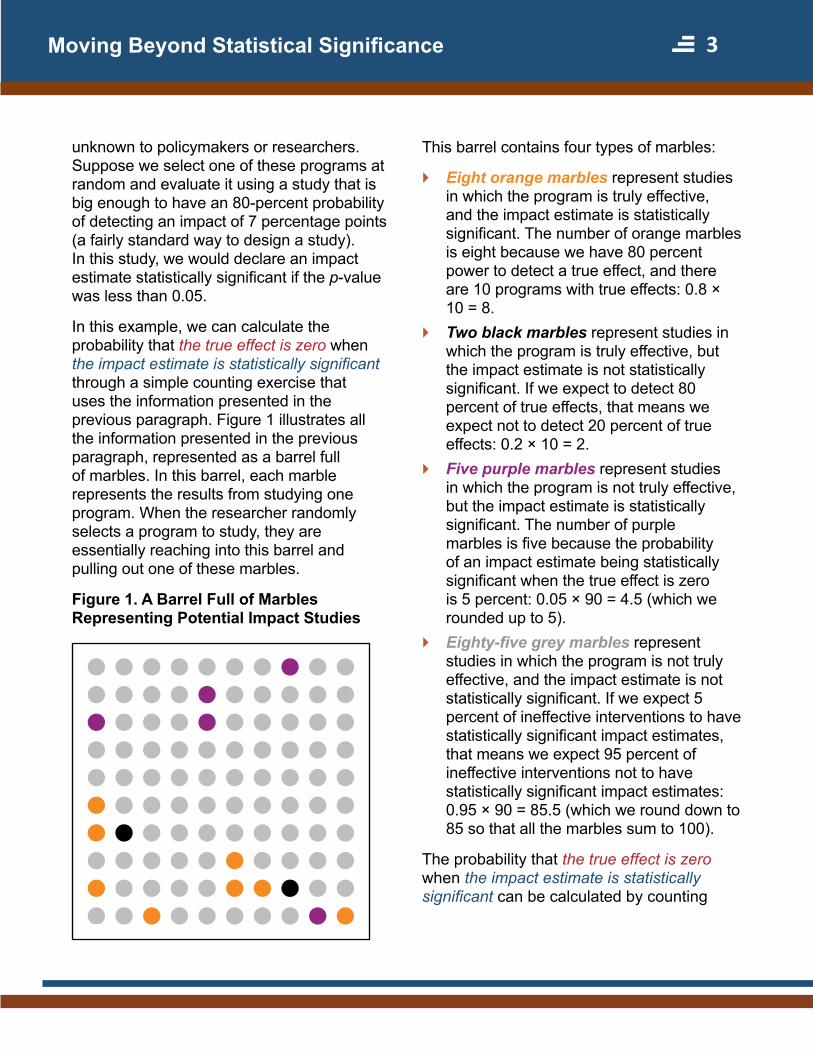
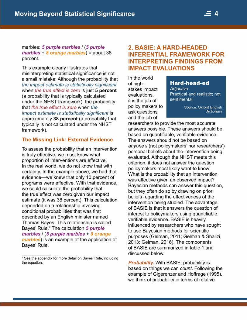
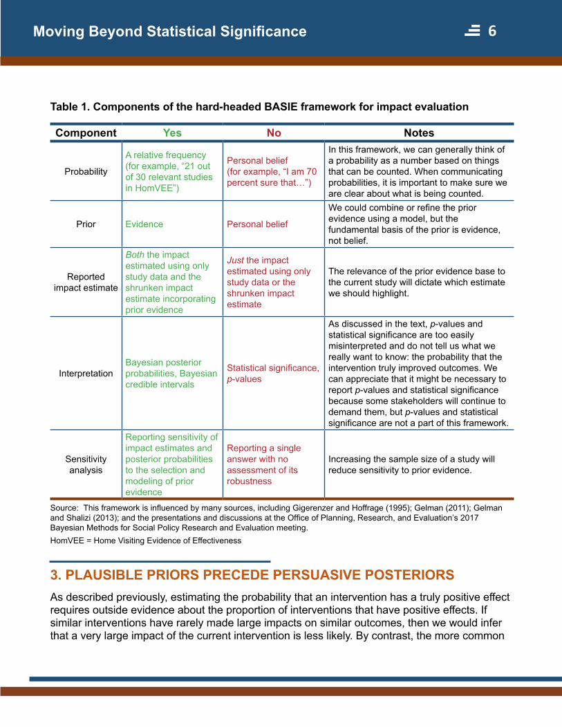
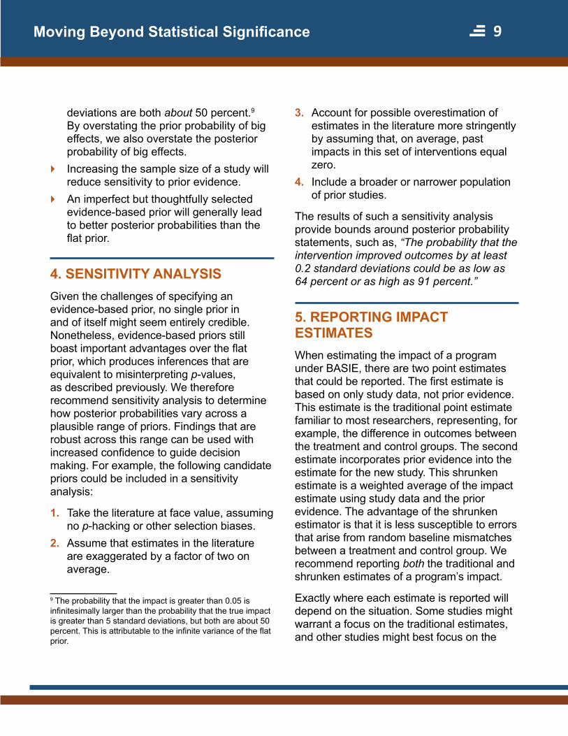
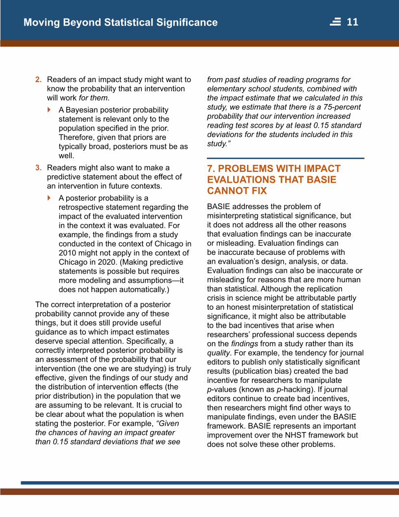
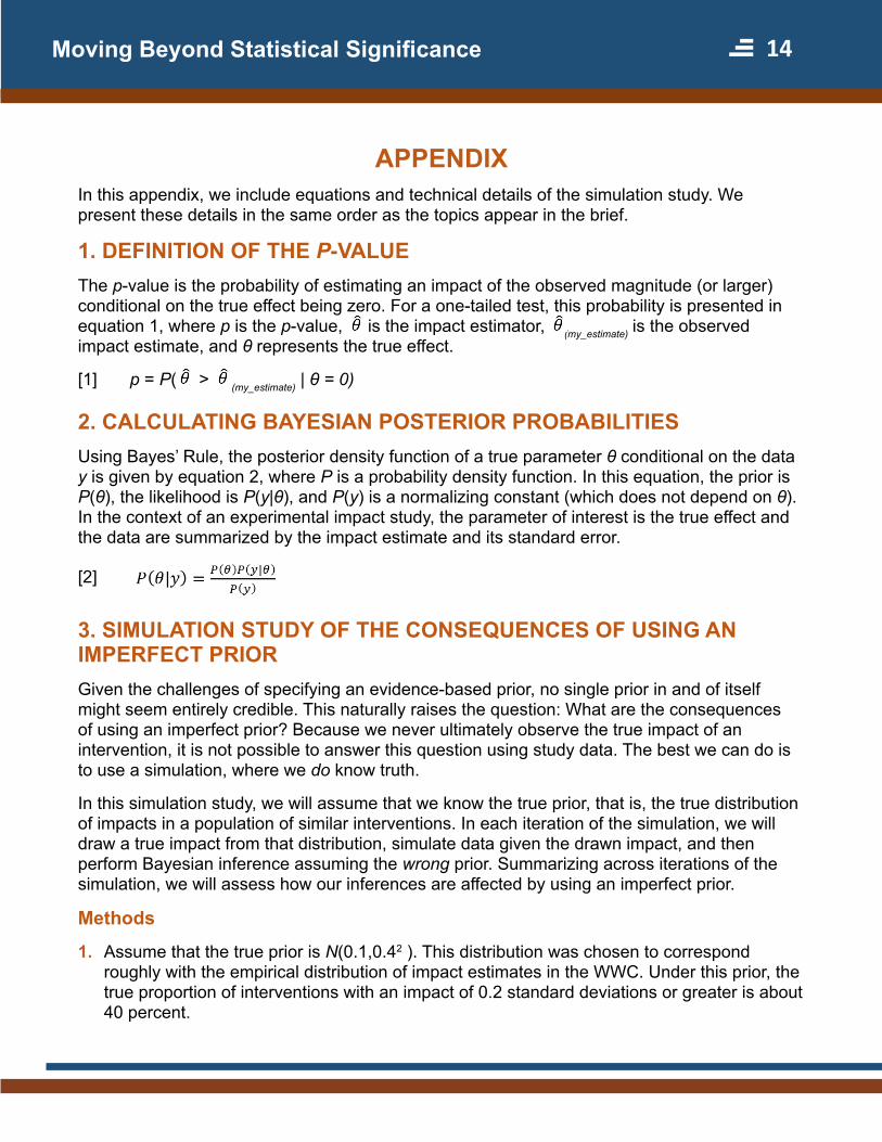
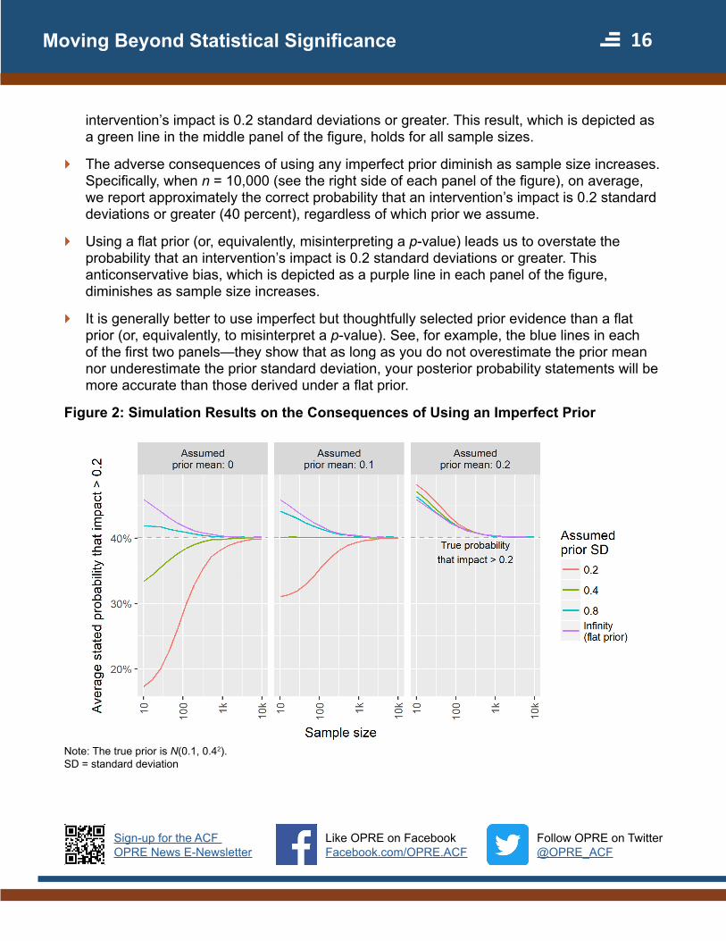