The Basics of Efficient SQL - Oracle · 121 6 The Basics of Efficient SQL In the previous chapter...
98
121 6 The Basics of Efficient SQL In the previous chapter we examined the basic syntax of SQL in Oracle Database. This chapter will attempt to detail the most simplistic aspects of SQL code tuning. In other words, we are going to discuss what in SQL statements is good for performance and what is not. The approach to performance in this chapter will be based on a purely SQL basis. We want to avoid the nitty-gritty and internal processing occurring in Oracle Database at this stage. It is essential to understand the basic facts about how to write well-performing SQL code first, without considering specific details of Oracle software. The most important rule of thumb with SQL statements, and particularly SELECT statements, those most subject to tuning, is what is commonly known as the “KISS” rule “Keep It Simple Stupid!” The simpler your SQL statements are the faster they will be. There are two reasons for this. Firstly, simple SQL statements are much more easily tuned and secondly, the Optimizer will function a lot bet- ter when assessing less complex SQL code. The negative effect of this is granularity but this negative effect depends on how the application is coded. For instance, connecting to and disconnecting from the database for every SQL code statement is extremely inefficient. Part of the approach in this chapter is to present SQL perform- ance examples without bombarding the reader with the details of too much theory and reference material. Any reference items such as explanations of producing query plans will be covered later on in this book. So what this chapter will cover is mostly a general type of SQL code tuning. Thus the title of this chapter: “The Basics of Efficient SQL.” Let’s start with a brief look at the SELECT statement.
Transcript of The Basics of Efficient SQL - Oracle · 121 6 The Basics of Efficient SQL In the previous chapter...

121
6The Basics of Efficient SQL
In the previous chapter we examined the basic syntax of SQL inOracle Database. This chapter will attempt to detail the mostsimplistic aspects of SQL code tuning. In other words, we are goingto discuss what in SQL statements is good for performance and whatis not. The approach to performance in this chapter will be based ona purely SQL basis. We want to avoid the nitty-gritty and internalprocessing occurring in Oracle Database at this stage. It is essentialto understand the basic facts about how to write well-performingSQL code first, without considering specific details of Oraclesoftware.
The most important rule of thumb with SQL statements, andparticularly SELECT statements, those most subject to tuning, iswhat is commonly known as the “KISS” rule “Keep It Simple Stupid!”The simpler your SQL statements are the faster they will be. Thereare two reasons for this. Firstly, simple SQL statements are muchmore easily tuned and secondly, the Optimizer will function a lot bet-ter when assessing less complex SQL code. The negative effect of thisis granularity but this negative effect depends on how the applicationis coded. For instance, connecting to and disconnecting from thedatabase for every SQL code statement is extremely inefficient.
Part of the approach in this chapter is to present SQL perform-ance examples without bombarding the reader with the details of toomuch theory and reference material. Any reference items such asexplanations of producing query plans will be covered later on in thisbook.
So what this chapter will cover is mostly a general type of SQLcode tuning. Thus the title of this chapter: “The Basics of EfficientSQL.” Let’s start with a brief look at the SELECT statement.

6.1 The SELECT Statement
It is always faster to SELECT exact column names. Thus using theEmployees schema
SELECT division_id, name, city, state, country FROM division;
is faster than
SELECT * FROM division;
Also since there is a primary key index on the Division table
SELECT division_id FROM division;
will only read the index file and should completely ignore the tableitself. Since the index contains only a single column and the tablecontains five columns, reading the index is faster because there is lessphysical space to traverse.
In order to prove these points we need to use the EXPLAIN PLANcommand. Oracle Database’s EXPLAIN PLAN command allows aquick peek into how the Oracle Database Optimizer will execute anSQL statement, displaying a query plan devised by the Optimizer.
The EXPLAIN PLAN command creates entries in the PLAN_TABLEfor a SELECT statement. The resulting query plan for the SELECTstatement following is shown after it. Various versions of the queryused to retrieve rows from the PLAN_TABLE, a hierarchical query,can be found in Appendix B. In order to use the EXPLAIN PLANcommand statistics must be generated. Both the EXPLAIN PLANcommand and statistics will be covered in detail in Chapter 9.
EXPLAIN PLAN SET statement_id='TEST' FOR SELECT * FROMdivision;
Query Cost Rows Bytes
SELECT STATEMENT on 1 10 460TABLE ACCESS FULL on DIVISION 1 10 460
One thing important to remember about the EXPLAIN PLANcommand is it produces a listed sequence of events, a query plan.Examine the following query and its query plan. The “Pos” or positionalcolumn gives a rough guide to the sequence of events that the Optimizerwill follow. In general, events will occur listed in the query plan frombottom to top, where additional indenting denotes containment.
6.1 The SELECT Statement 122

EXPLAIN PLAN SET statement_id='TEST' FORSELECT di.name, de.name, prj.name,SUM(prj.budget-prj.cost)
FROM division di JOIN department de USING(division_id)JOIN project prj USING(department_id)
GROUP BY di.name, de.name, prj.nameHAVING SUM(prj.budget-prj.cost) > 0;
Query Pos Cost Rows Bytes
SELECT STATEMENT on 97 97 250 17500FILTER on 1SORT GROUP BY on 1 97 250 17500HASH JOIN on 1 24 10000 700000TABLE ACCESS FULL on DIVISION 1 1 10 170HASH JOIN on 2 3 100 3600TABLE ACCESS FULL on DEPARTMENT 1 1 100 1900TABLE ACCESS FULL on PROJECT 2 13 10000 340000
Now let’s use the Accounts schema. The Accounts schema hassome very large tables. Large tables show differences between thecosts of data retrievals more easily. The GeneralLedger table con-tains over 700,000 rows at this point in time.
In the next example, we explicitly retrieve all columns from thetable using column names, similar to using SELECT * FROMGeneralLedger. Using the asterisk probably involves a small over-head in re-interpretation into a list of all column names, but this isinternal to Oracle Database and unless there are a huge number ofthese types of queries this is probably negligible.
EXPLAIN PLAN SET statement_id='TEST' FORSELECT generalledger_id,coa#,dr,cr,dte FROMgeneralledger;
The cost of retrieving 752,740 rows is 493 and the GeneralLedgertable is read in its entirety indicated by “TABLE ACCESS FULL”.
Query Cost Rows Bytes
SELECT STATEMENT on 493 752740 19571240TABLE ACCESS FULL on GENERALLEDGER 493 752740 19571240
Now we will retrieve only the primary key column from theGeneralLedger table.
EXPLAIN PLAN SET statement_id='TEST' FORSELECT generalledger_id FROM generalledger;
123 6.1 The SELECT Statement
Chapter 6

For the same number of rows the cost is reduced to 217 since thebyte value is reduced by reading the index only, using a form of a fullindex scan. This means that only the primary key index is being read,not the table.
Query Cost Rows Bytes
SELECT STATEMENT on 217 752740 4516440INDEX FAST FULL SCAN on XPKGENERALLEDGER 217 752740 4516440
Here is another example using an explicit column name but thisone has a greater difference in cost from that of the full table scan.This is because the column retrieved uses an index, which is physi-cally smaller than the index for the primary key. The index on theCOA# column is consistently 5 bytes in length for all rows. For theprimary key index only the first 9,999 rows have an index value ofless than 5 bytes in length.
EXPLAIN PLAN SET statement_id='TEST' FOR SELECT coa# FROM generalledger;
Query Cost Rows Bytes
SELECT STATEMENT on 5 752740 4516440INDEX FAST FULL SCAN on XFK_GL_COA# 5 752740 4516440
Following are two interesting examples utilizing a composite index.The structure of the index is built as the SEQ# column containedwithin the CHEQUE_ID column (CHEQUE_ID + SEQ#) and not theother way around. In older versions of Oracle Database this probablywould have been a problem. The Oracle9i Database Optimizer is nowmuch improved when matching poorly ordered SQL statementcolumns to existing indexes. Both examples use the same index. Theorder of columns is not necessarily a problem in Oracle9i Database.
Oracle Database 10g has Optimizer improvements such as lessof a need for SQL code statements to be case sensitive.
EXPLAIN PLAN SET statement_id='TEST' FORSELECT cheque_id, seq# FROM cashbookline;
Query Cost Rows Bytes
SELECT STATEMENT on 65 188185 1505480INDEX FAST FULL SCAN on XPKCASHBOOKLINE 65 188185 1505480
6.1 The SELECT Statement 124
10g

It can be seen that even with the columns selected in the reverseorder of the index, the index is still used.
EXPLAIN PLAN SET statement_id='TEST' FORSELECT seq#,cheque_id FROM cashbookline;
Query Cost Rows Bytes
SELECT STATEMENT on 65 188185 1505480INDEX FAST FULL SCAN on XPKCASHBOOKLINE 65 188185 1505480
The GeneralLedger table has a large number of rows. Now let’sexamine the idiosyncrasies of very small tables. There are some dif-ferences between the behavior of SQL when dealing with large andsmall tables.
In the next example, the Stock table is small and thus the costs ofreading the table or the index are the same. The first query, doing thefull table scan, reads around 20 times more physical space but thecost is the same. When tables are small the processing speed may notbe better when using indexes. Additionally when joining tablesthe Optimizer may very well choose to full scan a small static tablerather than read both index and table. The Optimizer may select thefull table scan as being quicker. This is often the case with genericstatic tables containing multiple types since they are typically readmore often.
EXPLAIN PLAN SET statement_id='TEST' FOR SELECT * FROMstock;
Query Cost Rows Bytes
SELECT STATEMENT on 1 118 9322TABLE ACCESS FULL on STOCK 1 118 9322
EXPLAIN PLAN SET statement_id='TEST' FOR SELECT stock_idFROM stock;
Query Cost Rows Bytes
SELECT STATEMENT on 1 118 472INDEX FULL SCAN on XPKSTOCK 1 118 472
So that is a brief look into how to tune simple SELECT state-ments. Try to use explicit columns and try to read columns in indexorders if possible, even to the point of reading indexes and nottables.
125 6.1 The SELECT Statement
Chapter 6

6.1.1 A Count of Rows in the Accounts Schema
I want to show a row count of all tables in the Accounts schema Ihave in my database. If you remember we have already statedthat larger tables are more likely to require use of indexes andsmaller tables are not. Since the Accounts schema has both largeand small tables, SELECT statements and various clauses executedagainst different tables will very much affect how those differenttables should be accessed in the interest of good performance.Current row counts for all tables in the Accounts schema are shownin Figure 6.1.
� Accounts schema row counts vary throughout this book since thedatabase is continually actively adding rows and occasionallyrecovered to the initial state shown in Figure 6.1. Relative rowcounts between tables remain constant.
6.1 The SELECT Statement 126
Figure 6.1Row Countsof Accounts
Schema Tables
6.1.2 Filtering with the WHERE Clause
Filtering the results of a SELECT statement with a WHERE clauseimplies retrieving only a subset of rows from a larger set of rows.The WHERE clause can be used to either include wanted rows,exclude unwanted rows or both.

Once again using the Employees schema, in the following SQLstatement we filter rows to include only those rows we want,retrieving only those rows with PROJECTTYPE values starting withthe letter “R”.
SELECT * FROM projecttype WHERE name LIKE 'R%';
Now we do the opposite and filter out rows we do not want. Weget everything with values not starting with the letter “R”.
SELECT * FROM projecttype WHERE name NOT LIKE 'R%';
How does the WHERE clause affect the performance of a SELECTstatement? If the sequence of expression comparisons in a WHEREclause can match an index it should. The WHERE clause in theSELECT statement above does not match an index and thus thewhole table will be read. Since the Employees schema ProjectTypetable is small, having only 11 rows, this is unimportant. However, inthe case of the Accounts schema, where many of the tables have largenumbers of rows, avoiding full table scans, and forcing index read-ing is important. Following is a single WHERE clause comparisoncondition example SELECT statement. We will once again show thecost of the query using the EXPLAIN PLAN command. This querydoes an exact match on a very large table by applying an exact valueto find a single row. Note the unique index scan and the low cost ofthe query.
EXPLAIN PLAN SET statement_id='TEST' FORSELECT * FROM stockmovement WHERE stockmovement_id =5000;
Query Cost Rows Bytes
SELECT STATEMENT on 3 1 24TABLE ACCESS BY INDEX ROWID on STOCKMOVEMENT 3 1 24INDEX UNIQUE SCAN on XPKSTOCKMOVEMENT 2 1
Now let’s compare the query above with an example which usesanother single column index but searches for many more rows thana single row. This example consists of two queries. The first querygives us the WHERE clause literal value for the second query. Theresult of the first query is displayed here.
127 6.1 The SELECT Statement
Chapter 6

SQL> SELECT coa#, COUNT(coa#) “Rows” FROM generalledgerGROUP BY coa#;
COA# Rows
30001 31008640003 6628441000 17351150001 16971760001 33142
Now let’s look at a query plan for the second query with theWHERE clause filter applied. The second query shown next finds allthe rows in one of the groups listed in the result shown above.
EXPLAIN PLAN SET statement_id='TEST' FORSELECT * FROM generalledger WHERE coa# = 40003;
Query Cost Rows Bytes
SELECT STATEMENT on 493 150548 3914248TABLE ACCESS FULL on GENERALLEDGER 493 150548 3914248
The query above has an interesting result because the table is fullyscanned. This is because the Optimizer considers it more efficient toread the entire table rather than use the index on the COA# columnto find specific columns in the table. This is because the WHEREclause will retrieve over 60,000 rows, just shy of 10% of the entireGeneralLedger table. Over 10% is enough to trigger the Optimizerto execute a full table scan.
In comparison to the above query the following two queries reada very small table, the first with a unique index hit, and the secondwith a full table scan as a result of the range comparison condition (<).In the second query, if the table were much larger possibly theOptimizer would have executed an index range scan and read theindex file. However, since the table is small the Optimizer considersreading the entire table as being faster than reading the index to findwhat could be more than a single row.
EXPLAIN PLAN SET statement_id='TEST' FORSELECT * FROM category WHERE category_id = 1;
Query Cost Rows Bytes
SELECT STATEMENT on 1 1 12TABLE ACCESS BY INDEX ROWID on CATEGORY 1 1 12INDEX UNIQUE SCAN on XPKCATEGORY 1
6.1 The SELECT Statement 128

EXPLAIN PLAN SET statement_id='TEST' FORSELECT * FROM category WHERE category_id < 2;
The costs of both index use and the full table scan are the samebecause the table is small.
Query Cost Rows Bytes
SELECT STATEMENT on 1 1 12TABLE ACCESS FULL on CATEGORY 1 1 12
So far we have looked at WHERE clauses containing single com-parison conditions. In tables where multiple column indexes existthere are other factors to consider. The following two queriesproduce exactly the same result. Note the unique index scan on theprimary key for both queries. As with the ordering of index columnsin the SELECT statement, in previous versions of Oracle it is possi-ble that the same result would not have occurred for the secondquery. This is because in the past the order of table column compar-ison conditions absolutely had to match the order of columns in anindex. In the past the second query shown would probably haveresulted in a full table scan. The Optimizer is now more intelligent inOracle9i Database.
Oracle Database 10g has Optimizer improvements such as lessof a need for SQL code statements to be case sensitive.
We had a similar result previously in this chapter using theCHEQUE_ID and SEQ# columns on the CashbookLine table. Thesame applies to the WHERE clause.
EXPLAIN PLAN SET statement_id='TEST' FORSELECT * FROM ordersline WHERE order_id = 3137 ANDseq# = 1;
Query Cost Rows Bytes
SELECT STATEMENT on 3 1 17TABLE ACCESS BY INDEX ROWID on ORDERSLINE 3 1 17INDEX UNIQUE SCAN on XPKORDERSLINE 2 1
EXPLAIN PLAN SET statement_id='TEST' FORSELECT * FROM ordersline WHERE seq# = 1 AND order_id= 3137;
129 6.1 The SELECT Statement
Chapter 6
10g
Query Cost Rows Bytes
SELECT STATEMENT on 3 1 17TABLE ACCESS BY INDEX ROWID on ORDERSLINE 3 1 17INDEX UNIQUE SCAN on XPKORDERSLINE 2 1
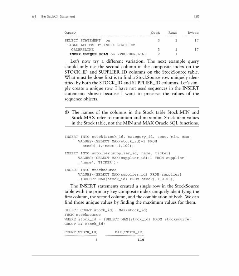
Let’s now try a different variation. The next example queryshould only use the second column in the composite index on theSTOCK_ID and SUPPLIER_ID columns on the StockSource table.What must be done first is to find a StockSource row uniquely iden-tified by both the STOCK_ID and SUPPLIER_ID columns. Let’s sim-ply create a unique row. I have not used sequences in the INSERTstatements shown because I want to preserve the values of thesequence objects.
� The names of the columns in the Stock table Stock.MIN andStock.MAX refer to minimum and maximum Stock item valuesin the Stock table, not the MIN and MAX Oracle SQL functions.
INSERT INTO stock(stock_id, category_id, text, min, max)VALUES((SELECT MAX(stock_id)+1 FROMstock),1,'text',1,100);
INSERT INTO supplier(supplier_id, name, ticker)VALUES((SELECT MAX(supplier_id)+1 FROM supplier),'name','TICKER');
INSERT INTO stocksourceVALUES((SELECT MAX(supplier_id) FROM supplier),(SELECT MAX(stock_id) FROM stock),100.00);
The INSERT statements created a single row in the StockSourcetable with the primary key composite index uniquely identifying thefirst column, the second column, and the combination of both. We canfind those unique values by finding the maximum values for them.
SELECT COUNT(stock_id), MAX(stock_id)FROM stocksourceWHERE stock_id = (SELECT MAX(stock_id) FROM stocksource)GROUP BY stock_id;
COUNT(STOCK_ID) MAX(STOCK_ID)
1 119
6.1 The SELECT Statement 130

SELECT COUNT(supplier_id), MAX(supplier_id)FROM stocksourceWHERE supplier_id = (SELECT MAX(supplier_id) FROM supplier)GROUP BY supplier_id;
COUNT(SUPPLIER_ID) MAX(SUPPLIER_ID)
1 3875
Now let’s attempt that unique index hit on the second column ofthe composite index in the StockSource table, amongst other combi-nations.
EXPLAIN PLAN SET statement_id='TEST' FORSELECT * FROM stocksource WHERE supplier_id = 3875;
Something very interesting happens. The foreign key index on theSUPPLIER_ID column is range scanned because the WHERE clauseis matched. The composite index is ignored.
Query Cost Rows Bytes
1. SELECT STATEMENT on 2 3 302. TABLE ACCESS BY INDEX ROWID on
STOCKSOURCE 2 3 303. INDEX RANGE SCAN on XFK_SS_SUPPLIER 1 3
The following query uses the STOCK_ID column, the first columnin the composite index. Once again, even though the STOCK_IDcolumn is the first column in the composite index the Optimizermatches the WHERE clause against the nonunique foreign key indexon the STOCK_ID column. Again the result is a range scan.
EXPLAIN PLAN SET statement_id='TEST' FORSELECT * FROM stocksource WHERE stock_id = 119;
Query Cost Rows Bytes
1. SELECT STATEMENT on 8 102 10202. TABLE ACCESS BY INDEX ROWID on
STOCKSOURCE 8 102 10203. INDEX RANGE SCAN on XFK_SS_STOCK 1 102
The next query executes a unique index hit on the compositeindex because the WHERE clause exactly matches the index.
EXPLAIN PLAN SET statement_id='TEST' FORSELECT * FROM stocksourceWHERE stock_id = 119 AND supplier_id = 3875;
131 6.1 The SELECT Statement
Chapter 6

Query Cost Rows Bytes
1. SELECT STATEMENT on 2 1 102. TABLE ACCESS BY INDEX ROWID on
STOCKSOURCE 2 1 103. INDEX UNIQUE SCAN on XPK_STOCKSOURCE 1 12084
Let’s clean up and delete the unique rows we created with theINSERT statements above. My script executing queries (seeAppendix B) on the PLAN_TABLE contains a COMMIT commandand thus ROLLBACK will not work.
DELETE FROM StockSource WHERE supplier_id = 3875 andstock_id = 119;
DELETE FROM supplier WHERE supplier_id = 3875;DELETE FROM stock WHERE stock_id = 119;COMMIT;
Now let’s do something slightly different. The purpose of creatingunique stock and supplier items in the StockSource table was to getthe best possibility of producing a unique index hit. If we were toselect from the StockSource table where more than a single rowexisted we would once again not get unique index hits. Dependingon the number of rows found we could get index range scans or evenfull table scans.
Firstly, find maximum and minimum counts for stocks duplicatedon the StockSource table.
SELECT * FROM(SELECT supplier_id, COUNT(supplier_id) AS suppliersFROM stocksource GROUP BY supplier_id ORDER BYsuppliers DESC)
WHERE ROWNUM = 1UNIONSELECT * FROM(
SELECT supplier_id, COUNT(supplier_id) AS suppliersFROM stocksource GROUP BY supplier_id ORDER BYsuppliers)
WHERE ROWNUM = 1;
There are nine suppliers with a SUPPLIER_ID column value of2711 and one with SUPPLIER_ID column value 2.
SUPPLIER_ID SUPPLIERS
2 12711 9
6.1 The SELECT Statement 132

Both the next two queries perform index range scans. If one of thequeries retrieved enough rows, as in the COA# = '40003' previouslyshown in this chapter, the Optimizer would force a read of the entiretable.
EXPLAIN PLAN SET statement_id='TEST' FORSELECT * FROM stocksource WHERE supplier_id = 2;
Query Cost Rows Bytes
1. SELECT STATEMENT on 2 3 302. TABLE ACCESS BY INDEX ROWID on
STOCKSOURCE 2 3 303. INDEX RANGE SCAN on XFK_SS_SUPPLIER 1 3
EXPLAIN PLAN SET statement_id='TEST' FORSELECT * FROM stocksource WHERE supplier_id = 2711;
Query Cost Rows Bytes
1. SELECT STATEMENT on 2 3 302. TABLE ACCESS BY INDEX ROWID on
STOCKSOURCE 2 3 303. INDEX RANGE SCAN on XFK_SS_SUPPLIER 1 3
So try to always do two things with WHERE clauses. Firstly, tryto match comparison condition column sequences with existing indexcolumn sequences, although it is not strictly necessary. Secondly,always try to use unique, single-column indexes wherever possible.A single-column unique index is much more likely to produce exacthits. An exact hit is the fastest access method.
6.1.3 Sorting with the ORDER BY Clause
The ORDER BY clause sorts the results of a query. The ORDER BYclause is always applied after all other clauses are applied, such asthe WHERE and GROUP BY clauses. Without an ORDER BYclause in an SQL statement, rows will often be retrieved in the physi-cal order in which they were added to the table. Rows are not alwaysappended to the end of a table as space can be reused. Therefore,physical row order is often useless. Additionally the sequence andcontent of columns in the SELECT statement, WHERE and GROUP BYclauses can also somewhat determine returned sort order to a certainextent.
133 6.1 The SELECT Statement
Chapter 6

In the following example we are sorting on the basis of the con-tent of the primary key index. Since the entire table is being readthere is no use of the index. Note the sorting applied to rowsretrieved from the table as a result of re-sorting applied by theORDER BY clause.
EXPLAIN PLAN SET statement_id='TEST' FORSELECT customer_id, name FROM customer ORDER BYcustomer_id;
Query Cost Rows Bytes Sort
SELECT STATEMENT on 25 2694 67350SORT ORDER BY on 25 2694 67350 205000TABLE ACCESS FULL on CUSTOMER 9 2694 67350
In the next example the name column is removed from the SELECTstatement and thus the primary key index is used. Specifying theCUSTOMER_ID column only in the SELECT statement forces useof the index, not the ORDER BY clause. Additionally there is nosorting because the index is already sorted in the required order.In this case the ORDER BY clause is unnecessary since an identicalresult would be obtained without it.
EXPLAIN PLAN SET statement_id='TEST' FORSELECT customer_id FROM customer ORDER BYcustomer_id;
Query Cost Rows Bytes Sort
SELECT STATEMENT on 6 2694 10776INDEX FULL SCAN on XPKCUSTOMER 6 2694 10776
The next example re-sorts the result by name. Again the wholetable is read so no index is used. The results are the same as for thequery before the previous one. Again there is physical sorting of therows retrieved from the table.
EXPLAIN PLAN SET statement_id='TEST' FORSELECT customer_id, name FROM customer ORDER BY name;
Query Cost Rows Bytes Sort
SELECT STATEMENT on 25 2694 67350SORT ORDER BY on 25 2694 67350 205000TABLE ACCESS FULL on CUSTOMER 9 2694 67350
6.1 The SELECT Statement 134

The ORDER BY clause will re-sort results.
Queries and sorts are now less case sensitive than in previousversions of Oracle Database.
Overriding WHERE with ORDER BY
The following example is interesting because the primary keycomposite index is used. Note that there is no sorting in the queryplan. It is unnecessary to sort since the index scanned is being readin the order required by the ORDER BY clause. In this case theOptimizer ignores the ORDER BY clause. The WHERE clause spec-ifies ORDER_ID only, for which there is a nonunique foreign keyindex. A nonunique index is appropriate to a range scan using the< range operator as shown in the example. However, the primary keycomposite index is used to search with, as specified in the ORDERBY clause. Thus the ORDER BY clause effectively overrides thespecification of the WHERE clause. The ORDER BY clause is oftenused to override any existing sorting parameters.
EXPLAIN PLAN SET statement_id='TEST' FORSELECT * FROM ordersline WHERE order_id < 10 ORDER BY order_id, seq#;
Query Cost Rows Bytes
SELECT STATEMENT on 4 3 51TABLE ACCESS BY INDEX ROWID on ORDERSLINE 4 3 51INDEX RANGE SCAN on XPKORDERSLINE 3 3
The second example excludes the overriding ORDER BY clause.Note how the index specified in the WHERE clause is utilized for anindex range scan. Thus in the absence of the ORDER BY clause inthe previous example the Optimizer resorts to the index specified inthe WHERE clause.
EXPLAIN PLAN SET statement_id='TEST' FORSELECT * FROM ordersline WHERE order_id < 10;
135 6.1 The SELECT Statement
Chapter 6
10g
Query Cost Rows Bytes
SELECT STATEMENT on 3 3 51TABLE ACCESS BY INDEX ROWID onORDERSLINE 3 3 51INDEX RANGE SCAN on XFK_ORDERLINE_ORDER 2 3
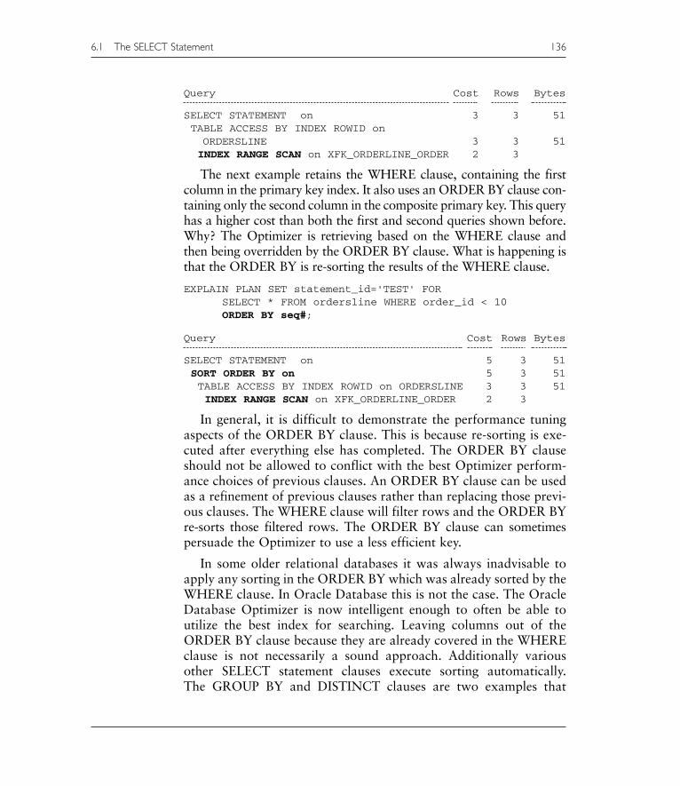
The next example retains the WHERE clause, containing the firstcolumn in the primary key index. It also uses an ORDER BY clause con-taining only the second column in the composite primary key. This queryhas a higher cost than both the first and second queries shown before.Why? The Optimizer is retrieving based on the WHERE clause andthen being overridden by the ORDER BY clause. What is happening isthat the ORDER BY is re-sorting the results of the WHERE clause.
EXPLAIN PLAN SET statement_id='TEST' FORSELECT * FROM ordersline WHERE order_id < 10ORDER BY seq#;
Query Cost Rows Bytes
SELECT STATEMENT on 5 3 51SORT ORDER BY on 5 3 51TABLE ACCESS BY INDEX ROWID on ORDERSLINE 3 3 51INDEX RANGE SCAN on XFK_ORDERLINE_ORDER 2 3
In general, it is difficult to demonstrate the performance tuningaspects of the ORDER BY clause. This is because re-sorting is exe-cuted after everything else has completed. The ORDER BY clauseshould not be allowed to conflict with the best Optimizer perform-ance choices of previous clauses. An ORDER BY clause can be usedas a refinement of previous clauses rather than replacing those previ-ous clauses. The WHERE clause will filter rows and the ORDER BYre-sorts those filtered rows. The ORDER BY clause can sometimespersuade the Optimizer to use a less efficient key.
In some older relational databases it was always inadvisable toapply any sorting in the ORDER BY which was already sorted by theWHERE clause. In Oracle Database this is not the case. The OracleDatabase Optimizer is now intelligent enough to often be able toutilize the best index for searching. Leaving columns out of theORDER BY clause because they are already covered in the WHEREclause is not necessarily a sound approach. Additionally variousother SELECT statement clauses execute sorting automatically.The GROUP BY and DISTINCT clauses are two examples that
6.1 The SELECT Statement 136

do inherent sorting. Use inherent sorting if possible rather thandoubling up with an ORDER BY clause.
So the ORDER BY clause is always executed after the WHEREclause. This does not mean that the Optimizer will choose either theWHERE clause or the ORDER BY clause as the best performingfactor. Try not to override the WHERE clause with the ORDER BYclause because the Optimizer may choose a less efficient method ofexecution based on the ORDER BY clause.
6.1.4 Grouping Result Sets
The GROUP BY clause can perform some inherent sorting. As withthe SELECT statement, WHERE clause and ORDER BY clause,matching of GROUP BY clause column sequences with index col-umn sequences is relevant to SQL code performance.
The first example aggregates based on the non-unique foreign keyon the ORDER_ID column. The aggregate is executed on theORDER_ID column into unique values for that ORDER_ID. Theforeign key index is the best performing option.
EXPLAIN PLAN SET statement_id='TEST' FORSELECT order_id, COUNT(order_id) FROM orderslineGROUP BY order_id;
The foreign key index is already sorted in the required order. TheNOSORT content in the SORT GROUP BY NOSORT on clauseimplies no sorting is required using the GROUP BY clause.
Query Cost Rows Bytes
SELECT STATEMENT on 26 172304 861520SORT GROUP BY NOSORT on 26 172304 861520INDEX FULL SCAN on XFK_ORDERLINE_ORDER 26 540827 2704135
The next example uses both columns in the primary key indexand thus the composite index is a better option. However, since thecomposite index is much larger in both size and rows the cost ismuch higher.
EXPLAIN PLAN SET statement_id='TEST' FORSELECT order_id, seq#, COUNT(order_id) FROM orderslineGROUP BY order_id, seq#;
137 6.1 The SELECT Statement
Chapter 6

Query Cost Rows Bytes
SELECT STATEMENT on 1217 540827 4326616SORT GROUP BY NOSORT on 1217 540827 4326616INDEX FULL SCAN on XPKORDERSLINE 1217 540827 4326616
In the next case we reverse the order of the columns in theGROUP BY sequence. As you can see there is no effect on cost since theOptimizer manages to match against the primary key composite index.
EXPLAIN PLAN SET statement_id='TEST' FORSELECT order_id, seq#, COUNT(order_id) FROM orderslineGROUP BY seq#, order_id;
Query Cost Rows Bytes
SELECT STATEMENT on 1217 540827 4326616SORT GROUP BY NOSORT on 1217 540827 4326616INDEX FULL SCAN on XPKORDERSLINE 1217 540827 4326616
Sorting with the GROUP BY Clause
This example uses a non-indexed column to aggregate. Thus thewhole table is accessed. Note that NOSORT is no longer included inthe SORT GROUP BY clause in the query plan. The GROUP BYclause is now performing sorting on the AMOUNT column.
EXPLAIN PLAN SET statement_id='TEST' FORSELECT amount, COUNT(amount) FROM orderslineGROUP BY amount;
Query Cost Rows Bytes Sort
SELECT STATEMENT on 4832 62371 374226SORT GROUP BY on 4832 62371 374226 7283000TABLE ACCESS FULL on ORDERSLINE 261 540827 3244962
Let’s examine GROUP BY clause sorting a little further.Sometimes it is possible to avoid sorting forced by the ORDER BYclause by ordering column names in the GROUP BY clause. Rowswill be sorted based on the contents of the GROUP BY clause.
EXPLAIN PLAN SET statement_id='TEST' FORSELECT amount, COUNT(amount) FROM orderslineGROUP BY amount ORDER BY amount;
In this case the ORDER BY clause is ignored.
6.1 The SELECT Statement 138

Query Cost Rows Bytes
1. SELECT STATEMENT on 6722 62371 3742262. SORT GROUP BY on 6722 62371 3742263. TABLE ACCESS FULL on ORDERSLINE 1023 540827 3244962
Inherent sorting in the GROUP BY clause can sometimes be usedto avoid extra sorting using an ORDER BY clause.
Using DISTINCT
DISTINCT retrieves the first value from a repeating group. Whenthere are multiple repeating groups DISTINCT will retrieve the firstrow from each group. Therefore, DISTINCT will always require asort. DISTINCT can operate on a single or multiple columns. Thefirst example executes the sort in order to find the first value in eachgroup. The second example has the DISTINCT clause removed anddoes not execute a sort. As a result the second example has a muchlower cost. DISTINCT will sort regardless.
EXPLAIN PLAN SET statement_id='TEST' FORSELECT DISTINCT(stock_id) FROM stockmovement;
Query Cost Rows Bytes
SELECT STATEMENT on 704 118 472SORT UNIQUE on 704 118 472INDEX FAST FULL SCAN on XFK_SM_STOCK 4 570175 2280700
EXPLAIN PLAN SET statement_id='TEST' FORSELECT stock_id FROM stockmovement;
Query Cost Rows Bytes
SELECT STATEMENT on 4 570175 2280700INDEX FAST FULL SCAN on XFK_SM_STOCK 4 570175 2280700
As far as performance tuning is concerned DISTINCT will alwaysrequire a sort. Sorting slows performance.
The HAVING Clause
Using the COUNT function as shown in the first two examples thereis little difference in performance. The slight difference is due to the
139 6.1 The SELECT Statement
Chapter 6
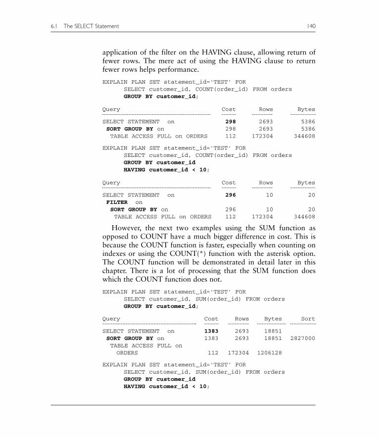
application of the filter on the HAVING clause, allowing return offewer rows. The mere act of using the HAVING clause to returnfewer rows helps performance.
EXPLAIN PLAN SET statement_id='TEST' FORSELECT customer_id, COUNT(order_id) FROM ordersGROUP BY customer_id;
Query Cost Rows Bytes
SELECT STATEMENT on 298 2693 5386SORT GROUP BY on 298 2693 5386TABLE ACCESS FULL on ORDERS 112 172304 344608
EXPLAIN PLAN SET statement_id='TEST' FORSELECT customer_id, COUNT(order_id) FROM ordersGROUP BY customer_idHAVING customer_id < 10;
Query Cost Rows Bytes
SELECT STATEMENT on 296 10 20FILTER onSORT GROUP BY on 296 10 20TABLE ACCESS FULL on ORDERS 112 172304 344608
However, the next two examples using the SUM function asopposed to COUNT have a much bigger difference in cost. This isbecause the COUNT function is faster, especially when counting onindexes or using the COUNT(*) function with the asterisk option.The COUNT function will be demonstrated in detail later in thischapter. There is a lot of processing that the SUM function doeswhich the COUNT function does not.
EXPLAIN PLAN SET statement_id='TEST' FORSELECT customer_id, SUM(order_id) FROM ordersGROUP BY customer_id;
Query Cost Rows Bytes Sort
SELECT STATEMENT on 1383 2693 18851SORT GROUP BY on 1383 2693 18851 2827000TABLE ACCESS FULL on ORDERS 112 172304 1206128
EXPLAIN PLAN SET statement_id='TEST' FORSELECT customer_id, SUM(order_id) FROM ordersGROUP BY customer_idHAVING customer_id < 10;
6.1 The SELECT Statement 140
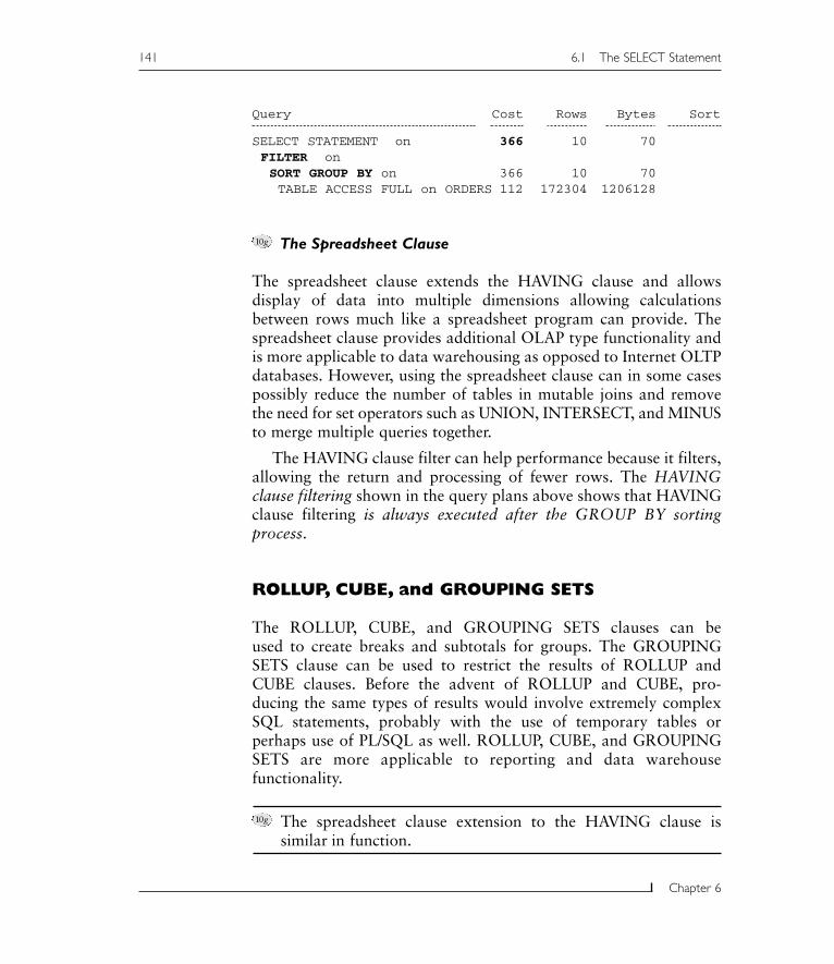
Query Cost Rows Bytes Sort
SELECT STATEMENT on 366 10 70FILTER onSORT GROUP BY on 366 10 70TABLE ACCESS FULL on ORDERS 112 172304 1206128
The Spreadsheet Clause
The spreadsheet clause extends the HAVING clause and allowsdisplay of data into multiple dimensions allowing calculationsbetween rows much like a spreadsheet program can provide. Thespreadsheet clause provides additional OLAP type functionality andis more applicable to data warehousing as opposed to Internet OLTPdatabases. However, using the spreadsheet clause can in some casespossibly reduce the number of tables in mutable joins and removethe need for set operators such as UNION, INTERSECT, and MINUSto merge multiple queries together.
The HAVING clause filter can help performance because it filters,allowing the return and processing of fewer rows. The HAVINGclause filtering shown in the query plans above shows that HAVINGclause filtering is always executed after the GROUP BY sortingprocess.
ROLLUP, CUBE, and GROUPING SETS
The ROLLUP, CUBE, and GROUPING SETS clauses can beused to create breaks and subtotals for groups. The GROUPINGSETS clause can be used to restrict the results of ROLLUP andCUBE clauses. Before the advent of ROLLUP and CUBE, pro-ducing the same types of results would involve extremely complexSQL statements, probably with the use of temporary tables orperhaps use of PL/SQL as well. ROLLUP, CUBE, and GROUPINGSETS are more applicable to reporting and data warehousefunctionality.
The spreadsheet clause extension to the HAVING clause issimilar in function.
141 6.1 The SELECT Statement
Chapter 6
10g
10g

The following examples simply show the use of the ROLLUP,CUBE, and GROUPING SETS clauses.
SELECT type, subtype, SUM(balance+ytd)FROM coaGROUP BY type, subtype;
SELECT type, subtype, SUM(balance+ytd)FROM coaGROUP BY ROLLUP (type, subtype);
SELECT type, subtype, SUM(balance+ytd)FROM coaGROUP BY CUBE (type, subtype);
SELECT type, subtype, SUM(balance+ytd)FROM coaGROUP BY GROUPING SETS ((type, subtype), (type),(subtype));
In general, the GROUP BY clause can perform some sorting if itmatches indexing. Filtering aggregate results with the HAVINGclause can help to increase performance by filtering aggregatedresults of the GROUP BY clause.
6.1.5 The FOR UPDATE Clause
The FOR UPDATE clause is a nice feature of SQL since it allowslocking of selected rows during a transaction. There are rare circum-stances where rows selected should be locked since there are depend-ent following changes in a single transaction, requiring selected datato remain the same during the course of that transaction.
SELECT …FOR UPDATE OF [ [schema.]table.]column [, … ] ][ NOWAIT | WAIT n ]
Note the two WAIT and NOWAIT options in the precedingsyntax. When a lock is encountered NOWAIT forces an abort. TheWAIT option will force a wait for a number of seconds. The defaultsimply waits until a row is available.
It should be obvious that with respect to tuning and concurrentmultiuser capability of applications the FOR UPDATE clause shouldbe avoided if possible. Perhaps the data model could be too granularthus necessitating the need to lock rows in various tables during thecourse of a transaction across multiple tables. Using the FORUPDATE clause is not good for the efficiency of SQL code in generaldue to potential locks and possible resulting waits for and by otherconcurrently executing transactions.
6.1 The SELECT Statement 142

6.2 Using Functions
The most relevant thing to say about functions is that they shouldnot be used where you expect an SQL statement to use an index.There are function-based indexes of course. A function-based indexcontains the resulting value of an expression. An index searchagainst that function-based index will search the index for the valueof the expression.
Let’s take a quick look at a few specific functions.
6.2.1 The COUNT Function
For older versions of Oracle Database the COUNT function hasbeen recommended as performing better when used in differentways. Prior to Oracle9i Database the COUNT(*) function using theasterisk was the fastest form because the asterisk option was specif-ically tuned to avoid any sorting. Let’s take a look at each of fourdifferent methods and show that they are all the same using both theEXPLAIN PLAN command and time testing. We will use theGeneralLedger table in the Accounts schema since it has the largestnumber of rows.
Notice how all the query plans for all the four following COUNTfunction options are identical. Additionally there is no sorting onanything but the resulting single row produced by the COUNTfunction, the sort on the aggregate.
Using the asterisk:
EXPLAIN PLAN SET statement_id='TEST' FORSELECT COUNT(*) FROM generalledger;
Query Cost Rows
1. SELECT STATEMENT on 382 12. SORT AGGREGATE on 13. INDEX FAST FULL SCAN on
XPK_GENERALLEDGER 382 752825
Forcing the use of a unique index:
EXPLAIN PLAN SET statement_id='TEST' FORSELECT COUNT(generalledger_id) FROMgeneralledger;
143 6.2 Using Functions
Chapter 6
Query Cost Rows
1. SELECT STATEMENT on 382 12. SORT AGGREGATE on 13. INDEX FAST FULL SCAN on XPK_GENERALLEDGER 382 752825
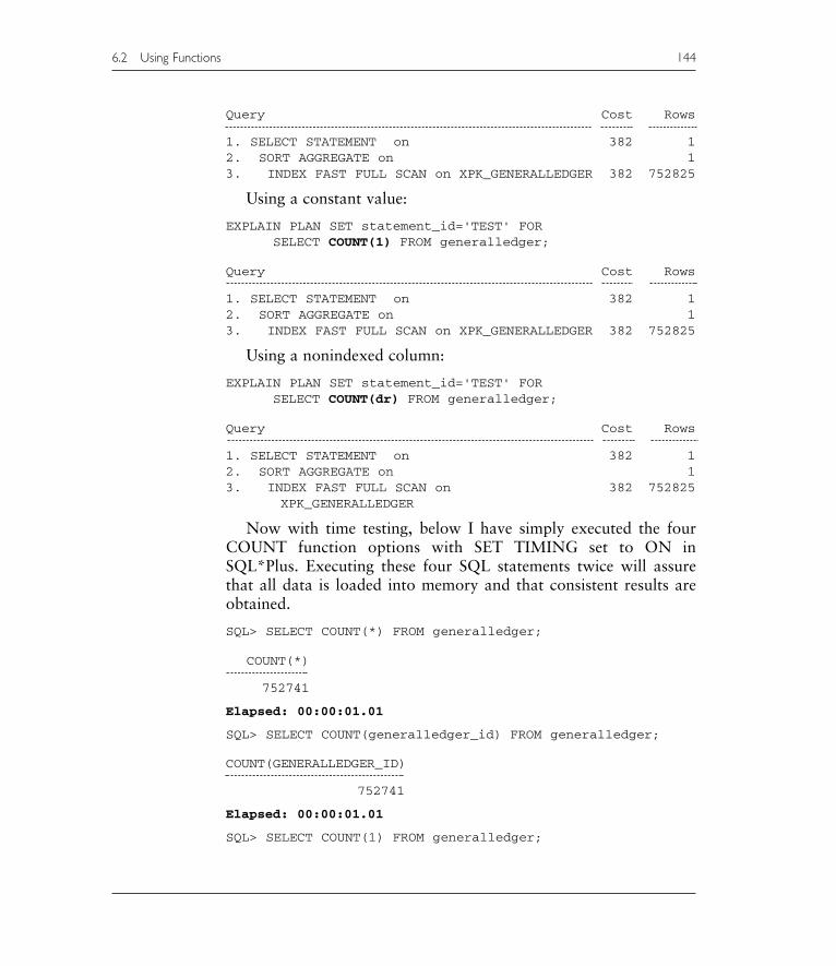
Using a constant value:
EXPLAIN PLAN SET statement_id='TEST' FORSELECT COUNT(1) FROM generalledger;
Query Cost Rows
1. SELECT STATEMENT on 382 12. SORT AGGREGATE on 13. INDEX FAST FULL SCAN on XPK_GENERALLEDGER 382 752825
Using a nonindexed column:
EXPLAIN PLAN SET statement_id='TEST' FORSELECT COUNT(dr) FROM generalledger;
Query Cost Rows
1. SELECT STATEMENT on 382 12. SORT AGGREGATE on 13. INDEX FAST FULL SCAN on 382 752825
XPK_GENERALLEDGER
Now with time testing, below I have simply executed the fourCOUNT function options with SET TIMING set to ON inSQL*Plus. Executing these four SQL statements twice will assurethat all data is loaded into memory and that consistent results areobtained.
SQL> SELECT COUNT(*) FROM generalledger;
COUNT(*)
752741
Elapsed: 00:00:01.01
SQL> SELECT COUNT(generalledger_id) FROM generalledger;
COUNT(GENERALLEDGER_ID)
752741
Elapsed: 00:00:01.01
SQL> SELECT COUNT(1) FROM generalledger;
6.2 Using Functions 144

COUNT(1)
752741
Elapsed: 00:00:01.01
SQL> SELECT COUNT(dr) FROM generalledger;
COUNT(DR)
752741
Elapsed: 00:00:01.01
As you can see from the time tests above, the COUNT functionwill perform the same no matter which method is used. In the latestversion of Oracle Database different forms of the COUNT functionwill perform identically. No form of the COUNT function is bettertuned than any other. All forms of the COUNT function perform thesame; using an asterisk, a constant or a column, regardless of columnindexing, the primary key index is always used.
6.2.2 The DECODE Function
DECODE can be used to replace composite SQL statements usinga set operator such as UNION. The Accounts Stock table has aQTYONHAND column. This column denotes how many items of aparticular stock item are currently in stock. Negative QTYONHANDvalues indicate that items have been ordered by customers but notyet received from suppliers.
The first example below uses four full reads of the Stock table andconcatenates the results together using UNION set operators.
EXPLAIN PLAN SET statement_id='TEST' FORSELECT stock_id||' Out of Stock' FROM stock WHEREqtyonhand <=0
UNIONSELECT stock_id||' Under Stocked' FROM stock
WHERE qtyonhand BETWEEN 1 AND min-1UNIONSELECT stock_id||' Stocked' FROM stock
WHERE qtyonhand BETWEEN min AND maxUNIONSELECT stock_id||' Over Stocked' FROM stock
WHERE qtyonhand > max;
145 6.2 Using Functions
Chapter 6

Query Pos Cost Rows Bytes
SELECT STATEMENT on 12 12 123 1543SORT UNIQUE on 1 12 123 1543UNION-ALL on 1TABLE ACCESS FULL on STOCK 1 1 4 32TABLE ACCESS FULL on STOCK 2 1 1 11TABLE ACCESS FULL on STOCK 3 1 28 420TABLE ACCESS FULL on STOCK 4 1 90 1080
This second example replaces the UNION set operators and thefour full table scan reads with a single full table scan using nestedDECODE functions. DECODE can be used to improve performance.
EXPLAIN PLAN SET statement_id='TEST' FORSELECT stock_id||' '||DECODE(SIGN(qtyonhand)
,-1,'Out of Stock',0,'Out of Stock',1,DECODE(SIGN(qtyonhand-min)
,-1,'Under Stocked',0,'Stocked',1,DECODE(sign(qtyonhand-max)
,-1,'Stocked',0,'Stocked',1,'Over Stocked'
))
) FROM stock;
Query Pos Cost Rows Bytes
SELECT STATEMENT on 1 1 118 1770TABLE ACCESS FULL on STOCK 1 1 118 1770
Using the DECODE function as a replacement for multiple queryset operators is good for performance but should only be used inextreme cases such as the UNION clause joined SQL statementsshown previously.
6.2.3 Datatype Conversions
Datatype conversions are a problem and will conflict with existingindexes unless function-based indexes are available and can becreated. Generally, if a function is executed in a WHERE clause, oranywhere else that can utilize an index, a full table scan is likely. Thisleads to inefficiency. There is some capability in Oracle SQL forimplicit datatype conversion but often use of functions in SQL
6.2 Using Functions 146

statements will cause the Optimizer to miss the use of indexes andperform poorly.
The most obvious datatype conversion concerns dates. Date fieldsin all the databases I have used are stored internally as a Julian number.A Julian number or date is an integer value from a database-specificdate measured in seconds. When retrieving a date value in a toolsuch as SQL*Plus there is usually a default date format. The internaldate value is converted to that default format. The conversion isimplicit, automatic, and transparent.
SELECT SYSDATE, TO_CHAR(SYSDATE,'J') “Julian” FROM DUAL;
SYSDATE Julian
03-MAR-03 2452702
Now for the sake of demonstration I will create an index on theGeneralLedger DTE column.
CREATE INDEX ak_gl_dte ON GENERALLEDGER(DTE);
Now obviously it is difficult to demonstrate an index hit with a keysuch as this because the date is a datestamp as well as a simple date.A simple date format such as MM/DD/YYYY excludes a timestamp.Simple dates and datestamps (timestamps) are almost impossible tomatch. Thus I will use SYSDATE in order to avoid a check against asimple formatted date. Both the GeneralLedger DTE column andSYSDATE are timestamps since the date column in the table wascreated using SYSDATE-generated values. We are only trying to showOptimizer query plans without finding rows.
The first example hits the new index I created and has a verylow cost.
EXPLAIN PLAN SET statement_id='TEST' FORSELECT * FROM generalledger WHERE dte = SYSDATE;
Query Cost Rows Bytes
SELECT STATEMENT on 2 593 15418TABLE ACCESS BY INDEX ROWID on GENERALLEDGER 2 593 15418INDEX RANGE SCAN on AK_GL_DTE 1 593
EXPLAIN PLAN SET statement_id='TEST' FORSELECT * FROM generalledgerWHERE TO_CHAR(dte, 'YYYY/MM/DD') = '2002/08/21';
147 6.2 Using Functions
Chapter 6

This second example does not hit the index because theTO_CHAR datatype conversion is completely inconsistent with thedatatype of the index. As a result the cost is much higher.
Query Cost Rows Bytes
SELECT STATEMENT on 493 7527 195702TABLE ACCESS FULL on GENERALLEDGER 493 7527 195702
Another factor to consider with datatype conversions is makingsure that datatype conversions are not placed onto columns. Convertliteral values not part of the database if possible. In order to demon-strate this I am going to add a zip code column to my Supplier table,create an index on that zip code column and regenerate statistics forthe Supplier table. I do not need to add values to the zip code col-umn to prove my point.
ALTER TABLE supplier ADD(zip NUMBER(5));CREATE INDEX ak_sp_zip ON supplier(zip);ANALYZE TABLE supplier COMPUTE STATISTICS;
Now we can show two examples. The first uses an index becausethere is no datatype conversion on the column in the table and the sec-ond reads the entire table because the conversion is on the column.
EXPLAIN PLAN SET statement_id='TEST' FORSELECT * FROM supplier WHERE zip = TO_NUMBER('94002');
Query Cost Rows Bytes
SELECT STATEMENT on 1 1 142TABLE ACCESS BY INDEX ROWID on SUPPLIER 1 1 142INDEX RANGE SCAN on AK_SP_ZIP 1 1
EXPLAIN PLAN SET statement_id='TEST' FORSELECT * FROM supplier WHERE TO_CHAR(zip) = '94002';
Query Cost Rows Bytes
SELECT STATEMENT on 13 1 142TABLE ACCESS FULL on SUPPLIER 13 1 142
Oracle SQL does not generally allow implicit type conversions butthere is some capacity for automatic conversion of strings to integers,if a string contains an integer value. Using implicit type conversionsis a very bad programming practice and is not recommended. A pro-grammer should never rely on another tool to do their job for them.Explicit coding is less likely to meet with potential errors in the future.
6.2 Using Functions 148

It is better to be precise since the computer will always be precise anddo exactly as you tell it to do. Implicit type conversion is included inOracle SQL for ease of programming. Ease of program coding is atop-down application to database design approach, totally contra-dictory to database tuning. Using a database from the point of viewof how the application can most easily be coded is not favorable toeventual production performance. Do not use implicit type conversions.As can be seen in the following examples implicit type conversionsdo not appear to make any difference to Optimizer costs.
EXPLAIN PLAN SET statement_id='TEST' FORSELECT * FROM supplier WHERE supplier_id = 3801;
Query Cost Rows Bytes
1. SELECT STATEMENT on 2 1 1422. TABLE ACCESS BY INDEX ROWID on SUPPLIER 2 1 1423. INDEX UNIQUE SCAN on XPK_SUPPLIER 1 3874
EXPLAIN PLAN SET statement_id='TEST' FORSELECT * FROM supplier WHERE supplier_id = '3801';
Query Cost Rows Bytes
1. SELECT STATEMENT on 2 1 1422. TABLE ACCESS BY INDEX ROWID on SUPPLIER 2 1 1423. INDEX UNIQUE SCAN on XPK_SUPPLIER 1 3874
In short, try to avoid using any type of data conversion functionin any part of an SQL statement which could potentially match anindex, especially if you are trying to assist performance by matchingappropriate indexes.
6.2.4 Using Functions in Queries
Now let’s expand on the use of functions by examining their use inall of the clauses of a SELECT statement.
Functions in the SELECT Statement
Firstly, let’s put a datatype conversion into a SELECT statement,which uses an index. As we can see in the two examples below, useof the index is not affected by the datatype conversion placed intothe SELECT statement.
149 6.2 Using Functions
Chapter 6

EXPLAIN PLAN SET statement_id='TEST' FORSELECT customer_id FROM customer;
Query Cost Rows Bytes
SELECT STATEMENT on 1 2694 10776INDEX FAST FULL SCAN on XPKCUSTOMER 1 2694 10776
EXPLAIN PLAN SET statement_id='TEST' FORSELECT TO_CHAR(customer_id) FROM customer;
Query Cost Rows Bytes
SELECT STATEMENT on 1 2694 10776INDEX FAST FULL SCAN on XPKCUSTOMER 1 2694 10776
Functions in the WHERE Clause
Now let’s examine the WHERE clause. In the two examples belowthe only difference is in the type of index scan utilized. Traditionallythe unique index hit produces an exact match and it should be faster.A later chapter will examine the difference between these two typesof index reads.
EXPLAIN PLAN SET statement_id='TEST' FORSELECT customer_id FROM customer WHEREcustomer_id = 100;
Query Cost Rows Bytes
SELECT STATEMENT on 1 1 4INDEX UNIQUE SCAN on XPKCUSTOMER 1 1 4
EXPLAIN PLAN SET statement_id='TEST' FORSELECT customer_id FROM customerWHERE TO_CHAR(customer_id) = '100';
Query Cost Rows Bytes
SELECT STATEMENT on 1 1 4INDEX FAST FULL SCAN on XPKCUSTOMER 1 1 4
Functions in the ORDER BY Clause
The ORDER BY clause can utilize indexing well, as already seen in thischapter, as long as WHERE clause index matching is not compromised.Let’s keep it simple. Looking at the following two examples it should
6.2 Using Functions 150

suffice to say that it might be a bad idea to include functions inORDER BY clauses. An index is not used in the second query andconsequently the cost is much higher.
EXPLAIN PLAN SET statement_id='TEST' FORSELECT * FROM generalledger ORDER BY coa#;
Query Cost Rows Bytes Sort
SELECT STATEMENT on 826 752740 19571240TABLE ACCESS BY INDEX ROWID on GL 826 752740 19571240INDEX FULL SCAN on XFK_GL_COA# 26 752740
EXPLAIN PLAN SET statement_id='TEST' FORSELECT * FROM generalledger ORDER BY TO_CHAR(coa#);
Query Cost Rows Bytes Sort
SELECT STATEMENT on 19070 752740 19571240SORT ORDER BY on 19070 752740 19571240 60474000TABLE ACCESS FULL onGENERALLEDGER 493 752740 19571240
Here is an interesting twist to using the same datatype conversionin the above two examples but with the conversion in the SELECTstatement and setting the ORDER BY clause to sort by positionrather than using the TO_CHAR(COA#) datatype conversion. Thereason why this example is lower in cost than the second example isbecause the conversion is done on selection and ORDER BY re-sorting is executed after data retrieval. In other words, in this exam-ple the ORDER BY clause does not affect the data access method.
EXPLAIN PLAN SET statement_id='TEST' FORSELECT TO_CHAR(coa#), dte, dr cr FROM generalledgerORDER BY 1;
Query Cost Rows Bytes Sort
SELECT STATEMENT on 12937 752740 13549320SORT ORDER BY on 12937 752740 13549320 42394000TABLE ACCESS FULL onGENERALLEDGER 493 752740 13549320
Functions in the GROUP BY Clause
Using functions in GROUP BY clauses will slow performance asshown in the following two examples.
151 6.2 Using Functions
Chapter 6

EXPLAIN PLAN SET statement_id='TEST' FORSELECT order_id, COUNT(order_id) FROM orderslineGROUP BY order_id;
Query Cost Rows Bytes
SELECT STATEMENT on 26 172304 861520SORT GROUP BY NOSORT on 26 172304 861520INDEX FULL SCAN onXFK_ORDERLINE_ORDER 26 540827 2704135
EXPLAIN PLAN SET statement_id='TEST' FORSELECT TO_CHAR(order_id), COUNT(order_id) FROMordersline
GROUP BY TO_CHAR(order_id);
Query Cost Rows Bytes Sort
SELECT STATEMENT on 3708 172304 861520SORT GROUP BY on 3708 172304 861520 8610000INDEX FAST FULL SCAN on XFK_ORDERLINE_ORDER 4 540827 2704135
When using functions in SQL statements it is best to keep thefunctions away from any columns involving index matching.
6.3 Pseudocolumns
There are some ways in which pseudocolumns can be used toincrease performance.
6.3.1 Sequences
A sequence is often used to create unique integer identifiers as pri-mary keys for tables. A sequence is a distinct database object and isaccessed as sequence.NEXTVAL and sequence.CURRVAL. Using theAccounts schema Supplier table we can show how a sequence is anefficient method in this case.
EXPLAIN PLAN SET statement_id='TEST' FORINSERT INTO supplier (supplier_id, name, ticker)VALUES(supplier_seq.NEXTVAL,'A new supplier', 'TICK');
Query Cost Rows Bytes
INSERT STATEMENT on 1 11 176SEQUENCE on SUPPLIER_SEQ
6.3 Pseudocolumns 152

EXPLAIN PLAN SET statement_id='TEST' FORINSERT INTO supplier (supplier_id, name, ticker)VALUES((SELECT MAX(supplier_id)+1FROM supplier), 'A new supplier', 'TICK');
Query Cost Rows Bytes
INSERT STATEMENT on 1 11 176
The query plan above is the same. There is a problem with it.Notice that a subquery is used to find the next SUPPLIER_ID value.This subquery is not evident in the query plan. Let’s do a query planfor the subquery as well.
EXPLAIN PLAN SET statement_id='TEST' FORSELECT MAX(supplier_id)+1 FROM supplier;
Query Cost Rows Bytes
1. SELECT STATEMENT on 2 1 32. SORT AGGREGATE on 1 33. INDEX FULL SCAN (MIN/MAX)
on XPK_SUPPLIER 2 3874 11622
We can see that the subquery will cause extra work. Since thequery plan seems to have difficulty with subqueries it is difficult totell the exact cost of using the subquery. Use sequences for uniqueinteger identifiers; they are centralized, more controllable, more eas-ily maintained, and perform better than other methods of counting.
6.3.2 ROWID Pointers
A ROWID is a logically unique database pointer to a row in a table.When a row is found using an index the index is searched. After therow is found in the index the ROWID is extracted from the indexand used to find the exact logical location of the row in its respectivetable. Accessing rows using the ROWID pseudocolumn is probablythe fastest row access method in Oracle Database since it is a directpointer to a unique address. The downside about ROWID pointers isthat they do not necessarily point at the same rows in perpetuity becausethey are relative to datafile, tablespace, block, and row. These valuescan change. Never store a ROWID in a table column as a pointer toother tables or rows if data or structure will be changing in the data-base. If ROWID pointers can be used for data access they can beblindingly fast but are not recommended by Oracle Corporation.
153 6.3 Pseudocolumns
Chapter 6

6.3.3 ROWNUM
A ROWNUM is a row number or a sequential counter representingthe order in which a row is returned from a query. ROWNUM canbe used to restrict the number of rows returned. There are numerousinteresting ways in which ROWNUM can be used. For instance, thefollowing example allows creation of a table from another, includingall constraints but excluding any rows. This is a useful and fastmethod of making an empty copy of a very large table.
CREATE TABLE tmp AS SELECT * FROM generalledger WHEREROWNUM < 1;
One point to note is as in the following example. A ROWNUMrestriction is applied in the WHERE clause. Since the ORDER BYclause occurs after the WHERE clause the ROWNUM restriction isnot applied to the sorted output. The solution to this problem is thesecond example.
SELECT * FROM customer WHERE ROWNUM < 25 ORDER BYname;
SELECT * FROM (SELECT * FROM customer ORDER BY name) WHEREROWNUM < 25;
6.4 Comparison Conditions
Different comparison conditions can have sometimes vastly differenteffects on the performance of SQL statements. Let’s examine eachin turn with various options and recommendations for potentialimprovement. The comparison conditions are listed here.
• Equi, anti, and range
• expr { [!]= | > | < | <= | >= } expr• expr [ NOT ] BETWEEN expr AND expr
• LIKE pattern matching
• expr [ NOT ] LIKE expr
• Set membership
• expr [ NOT ] IN expr• expr [ NOT ] EXISTS expr
6.4 Comparison Conditions 154

IN is now called an IN rather than a set membership conditionin order to limit confusion with object collection MEMBERconditions.
• Groups
• expr [ = | != | > | < | >= | <= ] [ ANY | SOME | ALL ] expr
6.4.1 Equi, Anti, and Range
Using an equals sign (equi) is the fastest comparison conditionif a unique index exists. Any type of anti comparison such as!= or NOT is looking for what is not in a table and thus mustread the entire table; sometimes full index scans can be used. Rangecomparisons scan indexes for ranges of rows. Let’s look at someexamples.
This example does a unique index hit; using the equals sign anexact hit single row is found.
EXPLAIN PLAN SET statement_id='TEST' FORSELECT * FROM generalledger WHERE generalledger_id =100;
Query Cost Rows Bytes
SELECT STATEMENT on 3 1 26TABLE ACCESS BY INDEX ROWID on GENERALLEDGER 3 1 26INDEX UNIQUE SCAN on XPKGENERALLEDGER 2 1
The anti (!=) comparison finds everything but the single rowspecified and thus must read the entire table.
EXPLAIN PLAN SET statement_id='TEST' FORSELECT * FROM generalledger WHERE generalledger_id !=100;
Query Pos Cost Rows Bytes
SELECT STATEMENT on 493 493 752739 19571214TABLE ACCESS FULL on GENERAL 1 493 752739 19571214
In the next case using the range (<) comparison searches a rangeof index values rather than a single unique index value.
155 6.4 Comparison Conditions
Chapter 6
10g

EXPLAIN PLAN SET statement_id='TEST' FORSELECT * FROM generalledger WHERE generalledger_id < 10;
Query Cost Rows Bytes
SELECT STATEMENT on 4 1 26TABLE ACCESS BY INDEX ROWID on GENERALLEDGE 4 1 26INDEX RANGE SCAN on XPKGENERALLEDGER 3 1
In the next example the whole table is read rather than using anindex range scan because most of the table will be read and thus theOptimizer considers reading the table as being faster.
EXPLAIN PLAN SET statement_id='TEST' FORSELECT * FROM generalledger WHERE generalledger_id >=100;
Query Pos Cost Rows Bytes
SELECT STATEMENT on 493 493 752740 19571240TABLE ACCESS FULL on GENERAL 1 493 752740 19571240
Here the BETWEEN comparison causes a range scan on an indexbecause the range of rows is small enough to not warrant a fulltable scan.
EXPLAIN PLAN SET statement_id='TEST' FORSELECT * FROM generalledgerWHERE generalledger_id BETWEEN 100 AND 200;
Query Cost Rows Bytes
SELECT STATEMENT on 4 1 26TABLE ACCESS BY INDEX ROWID on GENERALLEDGE 4 1 26INDEX RANGE SCAN on XPKGENERALLEDGER 3 1
6.4.2 LIKE Pattern Matching
The approach in the query plan used by the Optimizer will dependon how many rows are retrieved and how the pattern match isconstructed.
This query finds one row.
EXPLAIN PLAN SET statement_id='TEST' FORSELECT * FROM supplier WHERE name like '24/7 RealMedia, Inc.';
6.4 Comparison Conditions 156

Query Cost Rows Bytes
SELECT STATEMENT on 2 1 142TABLE ACCESS BY INDEX ROWID on SUPPLIER 2 1 142INDEX UNIQUE SCAN on AK_SUPPLIER_NAME 1 1
This query also retrieves a single row but there is a wildcardpattern match and thus a full table scan is the result.
EXPLAIN PLAN SET statement_id='TEST' FORSELECT * FROM supplier WHERE name LIKE '21st%';
Query Cost Rows Bytes
SELECT STATEMENT on 13 491 69722TABLE ACCESS FULL on SUPPLIER 13 491 69722
The next query finds almost 3,000 rows and thus a full scan ofthe table results regardless of the exactness of the pattern match.
� A pattern match using a % full wildcard pattern matchingcharacter anywhere in the pattern matching string will usuallyproduce a full table scan.
SQL> SELECT COUNT(*) FROM supplier WHERE name LIKE '%a%';
COUNT(*)
2926
EXPLAIN PLAN SET statement_id='TEST' FORSELECT * FROM supplier WHERE name LIKE '%a%';
Query Cost Rows Bytes
SELECT STATEMENT on 13 194 27548TABLE ACCESS FULL on SUPPLIER 13 194 27548
In general, since LIKE will match patterns which are in no wayrelated to indexes, LIKE will usually read an entire table.
6.4.3 Set Membership
IN should be used to test against literal values and EXISTS is oftenused to create a correlation between a calling query and a subquery.IN is best used as a pre-constructed set of literal values. IN willcause a subquery to be executed in its entirety before passing the
157 6.4 Comparison Conditions
Chapter 6
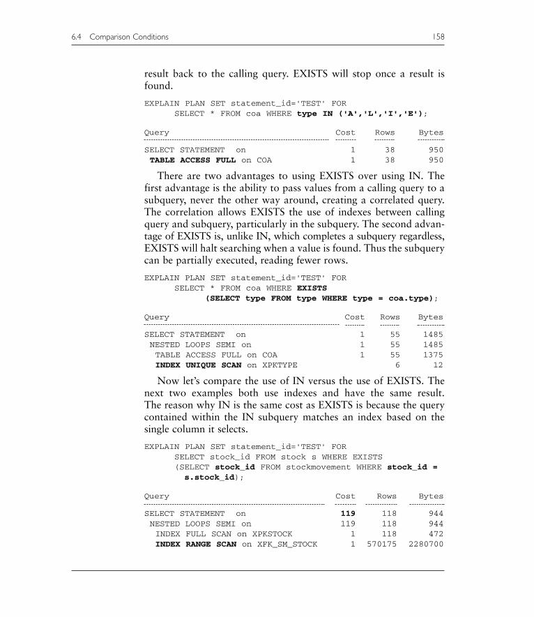
result back to the calling query. EXISTS will stop once a result isfound.
EXPLAIN PLAN SET statement_id='TEST' FORSELECT * FROM coa WHERE type IN ('A','L','I','E');
Query Cost Rows Bytes
SELECT STATEMENT on 1 38 950TABLE ACCESS FULL on COA 1 38 950
There are two advantages to using EXISTS over using IN. Thefirst advantage is the ability to pass values from a calling query to asubquery, never the other way around, creating a correlated query.The correlation allows EXISTS the use of indexes between callingquery and subquery, particularly in the subquery. The second advan-tage of EXISTS is, unlike IN, which completes a subquery regardless,EXISTS will halt searching when a value is found. Thus the subquerycan be partially executed, reading fewer rows.
EXPLAIN PLAN SET statement_id='TEST' FORSELECT * FROM coa WHERE EXISTS
(SELECT type FROM type WHERE type = coa.type);
Query Cost Rows Bytes
SELECT STATEMENT on 1 55 1485NESTED LOOPS SEMI on 1 55 1485TABLE ACCESS FULL on COA 1 55 1375INDEX UNIQUE SCAN on XPKTYPE 6 12
Now let’s compare the use of IN versus the use of EXISTS. Thenext two examples both use indexes and have the same result.The reason why IN is the same cost as EXISTS is because the querycontained within the IN subquery matches an index based on thesingle column it selects.
EXPLAIN PLAN SET statement_id='TEST' FORSELECT stock_id FROM stock s WHERE EXISTS(SELECT stock_id FROM stockmovement WHERE stock_id =s.stock_id);
Query Cost Rows Bytes
SELECT STATEMENT on 119 118 944NESTED LOOPS SEMI on 119 118 944INDEX FULL SCAN on XPKSTOCK 1 118 472INDEX RANGE SCAN on XFK_SM_STOCK 1 570175 2280700
6.4 Comparison Conditions 158

EXPLAIN PLAN SET statement_id='TEST' FORSELECT stock_id FROM stock WHERE stock_id IN(SELECT stock_id FROM stockmovement);
Query Cost Rows Bytes
SELECT STATEMENT on 119 118 944NESTED LOOPS SEMI on 119 118 944INDEX FULL SCAN on XPKSTOCK 1 118 472INDEX RANGE SCAN on XFK_SM_STOCK 1 570175 2280700
Now let’s do some different queries to show a very distinct dif-ference between IN and EXISTS. Note how the first example is muchlower in cost than the second. This is because the second optioncannot match indexes and executes two full table scans.
EXPLAIN PLAN SET statement_id='TEST' FORSELECT * FROM stockmovement sm WHERE EXISTS(SELECT * FROM stockmovement
WHERE stockmovement_id = sm.stockmovement_id);
Query Cost Rows Bytes Sort
SELECT STATEMENT on 8593 570175 16535075MERGE JOIN SEMI on 8593 570175 16535075TABLE ACCESS BY INDEXROWID on SM 3401 570175 13684200INDEX FULL SCAN onXPKSTOCKMOVEMENT 1071 570175
SORT UNIQUE on 5192 570175 2850875 13755000INDEX FAST FULL SCAN onXPKSTMOVE 163 570175 2850875
EXPLAIN PLAN SET statement_id='TEST' FORSELECT * FROM stockmovement sm WHERE qty IN
(SELECT qty FROM stockmovement);
Query Cost Rows Bytes Sort
SELECT STATEMENT on 16353 570175 15964900MERGE JOIN SEMI on 16353 570175 15964900SORT JOIN on 11979 570175 13684200 45802000TABLE ACCESS FULL onSTOCKMOVEMENT 355 570175 13684200
SORT UNIQUE on 4374 570175 2280700 13755000TABLE ACCESS FULL onSTOCKMOVEMENT 355 570175 2280700
Now let’s go yet another step further and restrict the calling queryto a single row result. What this will do is ensure that EXISTS
159 6.4 Comparison Conditions
Chapter 6

has the best possible chance of passing a single row identifier intothe subquery, thus ensuring a unique index hit in the subquery. TheStockMovement table has been joined to itself to facilitate thedemonstration of the difference between using EXISTS and IN. Notehow the IN subquery executes a full table scan and the EXISTSsubquery does not.
EXPLAIN PLAN SET statement_id='TEST' FORSELECT * FROM stockmovement smWHERE EXISTS(
SELECT qty FROM stockmovementWHERE stockmovement_id = sm.stockmovement_id)
AND stockmovement_id = 10;
Query Cost Rows Bytes
1. SELECT STATEMENT on 2 1 292. NESTED LOOPS SEMI on 2 1 293. TABLE ACCESS BY INDEX ROWID on
STOCKMOVEMENT 2 1 244. INDEX UNIQUE SCAN on
XPK_STOCKMOVEMENT 1 5701753. INDEX UNIQUE SCAN on
XPK_STOCKMOVEMENT 1 5
EXPLAIN PLAN SET statement_id='TEST' FORSELECT * FROM stockmovement smWHERE qty IN (SELECT qty FROMstockmovement)
AND stockmovement_id = 10;
Query Cost Rows Bytes
1. SELECT STATEMENT on 563 1 282. NESTED LOOPS SEMI on 563 1 283. TABLE ACCESS BY INDEX ROWID on
STOCKMOVEMENT 2 1 244. INDEX UNIQUE SCAN on
XPK_STOCKMOVEMENT 1 5701753. TABLE ACCESS FULL on
STOCKMOVEMENT 561 570175 2280700
The benefit of using EXISTS rather than IN for a subquerycomparison is that EXISTS can potentially find much fewer rowsthan IN. IN is best used with literal values and EXISTS is bestused as applying a fast access correlation between a calling and asubquery.
6.4 Comparison Conditions 160

6.4.4 Groups
ANY, SOME, and ALL comparisons are generally not very conduciveto SQL tuning. In some respects they are best not used.
6.5 Joins
A join is a combination of rows extracted from two or more tables.Joins can be very specific, for instance an intersection between twotables, or they can be less specific such as an outer join. An outer joinis a join returning an intersection plus rows from either or bothtables, not in the other table.
This discussion on tuning joins is divided into three sections: joinsyntax formats, efficient joins, and inefficient joins. Since this bookis about tuning it seems sensible to divide joins between efficientjoins and inefficient joins.
Firstly, let’s take a look at the two different available join syntaxformats in Oracle SQL.
6.5.1 Join Formats
There are two different syntax formats available for SQL joinqueries. The first is Oracle Corporation’s proprietary format and thesecond is the ANSI standard format. Let’s test the two formats to seeif either format can be tuned to the best performance.
The Oracle SQL proprietary format places join specifications intothe WHERE clause of an SQL query. The only syntactical additionto the standard SELECT statement syntax is the use of the (+) orouter join operator. We will deal with tuning outer joins later in thischapter. Following is an example of an Oracle SQL proprietary joinformatted query with its query plan, using the Employees schema.All tables are fully scanned because there is joining but no filtering.The Optimizer forces full table reads on all tables because it is thefastest access method to read all the data.
EXPLAIN PLAN SET statement_id='TEST' FORSELECT di.name, de.name, prj.nameFROM division di, department de, project prj
161 6.5 Joins
Chapter 6

WHERE di.division_id = de.division_idAND de.department_id = prj.department_id;
Query Cost Rows Bytes
SELECT STATEMENT on 23 10000 640000HASH JOIN on 23 10000 640000HASH JOIN on 3 100 3600TABLE ACCESS FULL on DIVISION 1 10 170TABLE ACCESS FULL on DEPARTMENT 1 100 1900
TABLE ACCESS FULL on PROJECT 13 10000 280000
The next example shows the same query except using the ANSIstandard join format. Notice how the query plan is identical.
EXPLAIN PLAN SET statement_id='TEST' FORSELECT di.name, de.name, prj.nameFROM division di JOIN department deUSING(division_id)
JOIN project prj USING (department_id);
Query Cost Rows Bytes
SELECT STATEMENT on 23 10000 640000HASH JOIN on 23 10000 640000HASH JOIN on 3 100 3600TABLE ACCESS FULL on DIVISION 1 10 170TABLE ACCESS FULL on DEPARTMENT 1 100 1900
TABLE ACCESS FULL on PROJECT 13 10000 280000
What is the objective of showing the two queries above, includingtheir query plan details? The task of this book is performance tuning.Is either of the two of Oracle SQL proprietary or ANSI join formatsinherently faster? Let’s try to prove it either way. Once again theOracle SQL proprietary format is shown below but with a filter added,finding only a single row in the join.
EXPLAIN PLAN SET statement_id='TEST' FORSELECT di.name, de.name, prj.nameFROM division di, department de, project prjWHERE di.division_id = 5AND di.division_id = de.division_idAND de.department_id = prj.department_id;
Query Cost Rows Bytes
SELECT STATEMENT on 4 143 9152TABLE ACCESS BY INDEX ROWID on PROJECT 2 10000 280000NESTED LOOPS on 4 143 9152
6.5 Joins 162
NESTED LOOPS on 2 1 36TABLE ACCESS BY INDEX ROWID on DIVISION 1 1 17INDEX UNIQUE SCAN on XPKDIVISION 1
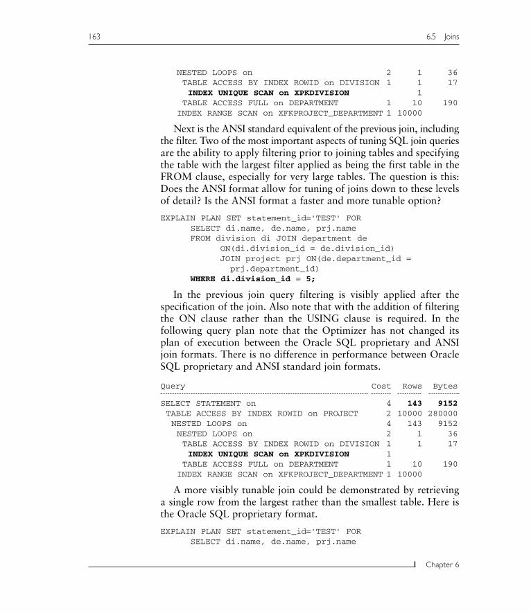
TABLE ACCESS FULL on DEPARTMENT 1 10 190INDEX RANGE SCAN on XFKPROJECT_DEPARTMENT 1 10000
Next is the ANSI standard equivalent of the previous join, includingthe filter. Two of the most important aspects of tuning SQL join queriesare the ability to apply filtering prior to joining tables and specifyingthe table with the largest filter applied as being the first table in theFROM clause, especially for very large tables. The question is this:Does the ANSI format allow for tuning of joins down to these levelsof detail? Is the ANSI format a faster and more tunable option?
EXPLAIN PLAN SET statement_id='TEST' FORSELECT di.name, de.name, prj.nameFROM division di JOIN department de
ON(di.division_id = de.division_id)JOIN project prj ON(de.department_id =prj.department_id)
WHERE di.division_id = 5;
In the previous join query filtering is visibly applied after thespecification of the join. Also note that with the addition of filteringthe ON clause rather than the USING clause is required. In thefollowing query plan note that the Optimizer has not changed itsplan of execution between the Oracle SQL proprietary and ANSIjoin formats. There is no difference in performance between OracleSQL proprietary and ANSI standard join formats.
Query Cost Rows Bytes
SELECT STATEMENT on 4 143 9152TABLE ACCESS BY INDEX ROWID on PROJECT 2 10000 280000NESTED LOOPS on 4 143 9152NESTED LOOPS on 2 1 36TABLE ACCESS BY INDEX ROWID on DIVISION 1 1 17INDEX UNIQUE SCAN on XPKDIVISION 1
TABLE ACCESS FULL on DEPARTMENT 1 10 190INDEX RANGE SCAN on XFKPROJECT_DEPARTMENT 1 10000
A more visibly tunable join could be demonstrated by retrievinga single row from the largest rather than the smallest table. Here isthe Oracle SQL proprietary format.
EXPLAIN PLAN SET statement_id='TEST' FORSELECT di.name, de.name, prj.name
163 6.5 Joins
Chapter 6

FROM project prj, department de, division diWHERE prj.project_id = 50AND de.department_id = prj.department_idAND di.division_id = de.division_id;
Notice in the following query plan that the cost is the same butthe number of rows and bytes read are substantially reduced; only asingle row is retrieved. Since the Project table is being reduced in sizemore than any other table it appears first in the FROM clause. Thesame applies to the Department table being larger than the Divisiontable.
Query Cost Rows Bytes
SELECT STATEMENT on 4 1 67NESTED LOOPS on 4 1 67NESTED LOOPS on 3 1 50TABLE ACCESS BY INDEX ROWID on PROJECT 2 1 31INDEX UNIQUE SCAN on XPKPROJECT 1 1
TABLE ACCESS BY INDEX ROWID onDEPARTMENT 1 100 1900INDEX UNIQUE SCAN on XPKDEPARTMENT 100
TABLE ACCESS BY INDEX ROWID on DIVISION 1 10 170INDEX UNIQUE SCAN on XPKDIVISION 10
Now let’s do the same query but with the ANSI join format. Fromthe following query plan we can once again see that use of either theOracle SQL proprietary or ANSI join format does not appear tomake any difference to performance and capacity for tuning.
EXPLAIN PLAN SET statement_id='TEST' FORSELECT di.name, de.name, prj.nameFROM project prj JOIN department de
ON(prj.department_id = de.department_id)JOIN division di ON(de.division_id =di.division_id)
WHERE prj.project_id = 50;
Query Cost Rows Bytes
SELECT STATEMENT on 4 1 67NESTED LOOPS on 4 1 67NESTED LOOPS on 3 1 50TABLE ACCESS BY INDEX ROWID on PROJECT 2 1 31INDEX UNIQUE SCAN on XPKPROJECT 1 1
TABLE ACCESS BY INDEX ROWID onDEPARTMENT 1 100 1900
6.5 Joins 164
INDEX UNIQUE SCAN on XPKDEPARTMENT 100TABLE ACCESS BY INDEX ROWID on DIVISION 1 10 170INDEX UNIQUE SCAN on XPKDIVISION 10
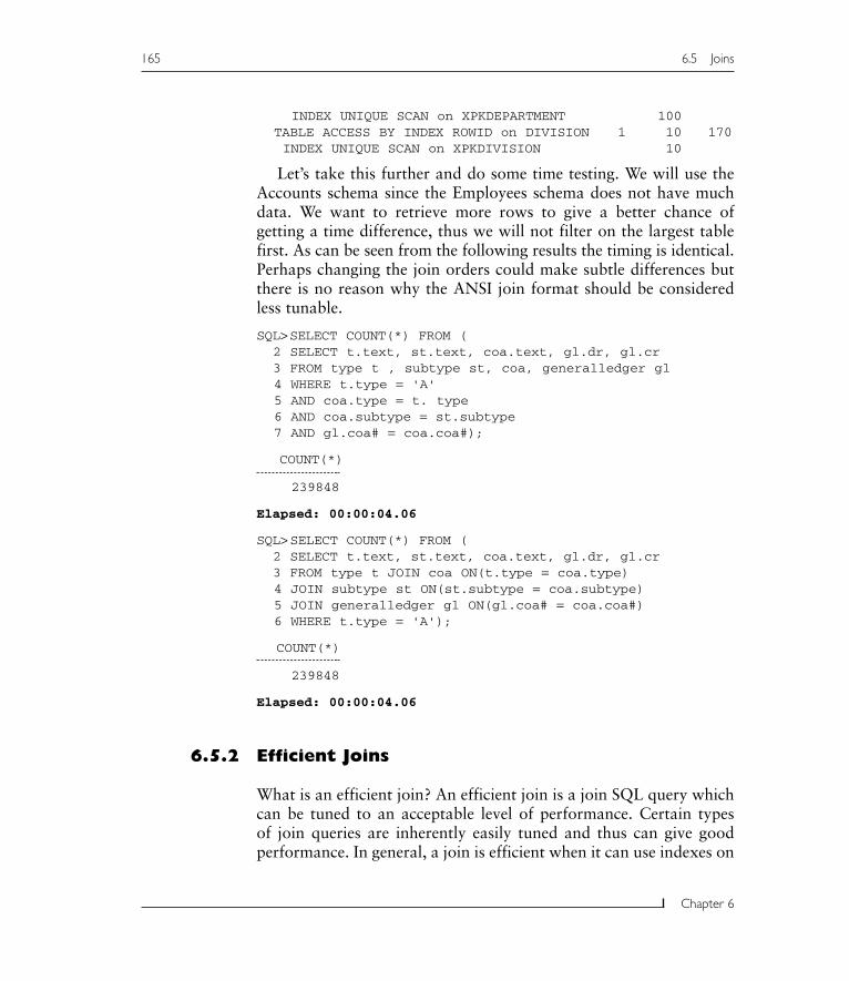
Let’s take this further and do some time testing. We will use theAccounts schema since the Employees schema does not have muchdata. We want to retrieve more rows to give a better chance ofgetting a time difference, thus we will not filter on the largest tablefirst. As can be seen from the following results the timing is identical.Perhaps changing the join orders could make subtle differences butthere is no reason why the ANSI join format should be consideredless tunable.
SQL>SELECT COUNT(*) FROM (2 SELECT t.text, st.text, coa.text, gl.dr, gl.cr3 FROM type t , subtype st, coa, generalledger gl4 WHERE t.type = 'A'5 AND coa.type = t. type6 AND coa.subtype = st.subtype7 AND gl.coa# = coa.coa#);
COUNT(*)
239848
Elapsed: 00:00:04.06
SQL>SELECT COUNT(*) FROM (2 SELECT t.text, st.text, coa.text, gl.dr, gl.cr3 FROM type t JOIN coa ON(t.type = coa.type)4 JOIN subtype st ON(st.subtype = coa.subtype)5 JOIN generalledger gl ON(gl.coa# = coa.coa#)6 WHERE t.type = 'A');
COUNT(*)
239848
Elapsed: 00:00:04.06
6.5.2 Efficient Joins
What is an efficient join? An efficient join is a join SQL query whichcan be tuned to an acceptable level of performance. Certain typesof join queries are inherently easily tuned and thus can give goodperformance. In general, a join is efficient when it can use indexes on
165 6.5 Joins
Chapter 6

large tables or is reading only very small tables. Moreover, any typeof join will be inefficient if coded improperly.
Intersections
An inner or natural join is an intersection between two tables. In Setparlance an intersection contains all elements occurring in both of thesets, or common to both sets. An intersection is efficient when indexcolumns are matched together in join clauses. Obviously intersectionmatching not using indexed columns will be inefficient. In that caseyou may want to create alternate indexes. On the other hand, whena table is very small the Optimizer may conclude that reading thewhole table is faster than reading an associated index plus the table.How the Optimizer makes a decision such as this will be discussedin later chapters since this subject matter delves into indexing andphysical file block structure in Oracle Database datafiles.
In the example below both of the Type and COA tables are sosmall that the Optimizer does not bother with the indexes and sim-ply reads both of the tables fully.
EXPLAIN PLAN SET statement_id='TEST' FORSELECT t.text, coa.text FROM type t JOIN coaUSING(type);
Query Cost Rows Bytes
SELECT STATEMENT on 3 55 1430HASH JOIN on 3 55 1430TABLE ACCESS FULL on TYPE 1 6 54TABLE ACCESS FULL on COA 1 55 935
With the next example the Optimizer has done something a littleodd by using a unique index on the Subtype table. The Subtype tablehas only four rows and is extremely small.
EXPLAIN PLAN SET statement_id='TEST' FORSELECT t.text, coa.text FROM type t JOIN coaUSING(type)
JOIN subtype st USING(subtype);
Query Cost Rows Bytes
SELECT STATEMENT on 3 55 1650NESTED LOOPS on 3 55 1650
6.5 Joins 166

HASH JOIN on 3 55 1540TABLE ACCESS FULL on TYPE 1 6 54
TABLE ACCESS FULL on COA 1 55 1045INDEX UNIQUE SCAN on XPKSUBTYPE 4 8
Once again in the following example the Optimizer has chosento read the index for the very small Subtype table. However, theGeneralLedger table has its index read because it is very large andthe Optimizer considers that more efficient. The reason for this isthat the GeneralLedger table does have an index on the COA#column and thus the index is range scanned.
EXPLAIN PLAN SET statement_id='TEST' FORSELECT t.text, coa.textFROM type t JOIN coa USING(type)
JOIN subtype st USING(subtype)JOIN generalledger gl ON(gl.coa# =coa.coa#);
Query Cost Rows Bytes
SELECT STATEMENT on 58 752740 31615080NESTED LOOPS on 58 752740 31615080NESTED LOOPS on 3 55 1980HASH JOIN on 3 55 1870TABLE ACCESS FULL on TYPE 1 6 54TABLE ACCESS FULL on COA 1 55 1375
INDEX UNIQUE SCAN on XPKSUBTYPE 4 8INDEX RANGE SCAN on XFK_GL_COA# 1 752740 4516440
The most efficient type of inner join will generally be one retriev-ing very specific rows such as that in the next example. Most SQL ismore efficient when retrieving very specific, small numbers of rows.
EXPLAIN PLAN SET statement_id='TEST' FORSELECT t.text, st.text, coa.text, gl.dr, gl.crFROM generalledger gl JOIN coa ON(gl.coa# = coa.coa#)
JOIN type t ON(t.type = coa.type)JOIN subtype st ON(st.subtype =coa.subtype)
WHERE gl.generalledger_id = 100;
Note how all tables in the query plan are accessed using uniqueindex hits.
Query Pos Cost Rows Bytes
SELECT STATEMENT on 6 6 1 64NESTED LOOPS on 1 6 1 64
167 6.5 Joins
Chapter 6

NESTED LOOPS on 1 5 1 55NESTED LOOPS on 1 4 1 45TABLE ACCESS BY INDEX ROWID on GENE 1 3 1 20INDEX UNIQUE SCAN on XPKGENERALLED 1 2 1
TABLE ACCESS BY INDEX ROWID on COA 2 1 55 1375INDEX UNIQUE SCAN on XPKCOA 1 55
TABLE ACCESS BY INDEX ROWID on SUBTY 2 1 4 40INDEX UNIQUE SCAN on XPKSUBTYPE 1 4
TABLE ACCESS BY INDEX ROWID on TYPE 2 1 6 54INDEX UNIQUE SCAN on XPKTYPE 1 6
Self Joins
A self join joins a table to itself. Sometimes self-joining tables can behandled with hierarchical queries. Otherwise a self join is applied toa table containing columns within each row which link to each other.The Employee table in the Employees schema is such a table. Sinceboth the MANAGER_ID and EMPLOYEE_ID columns are indexedit would be fairly efficient to join the tables using those two columns.
EXPLAIN PLAN SET statement_id='TEST' FORSELECT manager.name, employee.nameFROM employee manager, employee employeeWHERE employee.manager_id = manager.employee_id;
In the query plan the Employee table is fully scanned twicebecause all the data is read and the Optimizer considers this fasterbecause the Employee table is small.
Query Cost Rows Bytes
SELECT STATEMENT on 3 110 2970HASH JOIN on 3 110 2970TABLE ACCESS FULL on EMPLOYEE 1 111 1554TABLE ACCESS FULL on EMPLOYEE 1 111 1443
Equi-Joins and Range Joins
An equi-join uses the equals sign (=) and a range join uses rangeoperators (<, >, <=, >=) and the BETWEEN operator. In general, the= operator will execute an exact row hit on an index and thus useunique index hits. The range operators will usually require theOptimizer to execute index range scans. BTree (binary tree) indexes,
6.5 Joins 168

the most commonly used indexes in Oracle Database, are highlyamenable to range scans. A BTree index is little like a limited depthtree and is optimized for both unique hits and range scans.
Going back into the Accounts schema, this first query uses twounique index hits. The filter helps that happen.
EXPLAIN PLAN SET statement_id='TEST' FORSELECT coa.*, gl.*FROM generalledger gl JOIN coa ON(gl.coa# = coa.coa#)WHERE generalledger_id = 10;
Query Cost Rows Bytes
SELECT STATEMENT on 4 1 51NESTED LOOPS on 4 1 51TABLE ACCESS BY INDEX ROWID onGENERALLEDG 3 1 26INDEX UNIQUE SCAN on XPKGENERALLEDGER 2 1
TABLE ACCESS BY INDEX ROWID on COA 1 55 1375INDEX UNIQUE SCAN on XPKCOA 55
This second query uses a range index scan on the GeneralLedgertable as a result of the range operator in the filter. Do you notice thatthe join clause inside the ON clause is where the range join operatoris placed? Well there isn’t really much point in joining ON (gl.coa#>= coa.coa#). I do not think I have ever seen an SQL join joiningusing a range operator. The result would be a very unusual type ofouter join perhaps. Thus there is no need for a query plan.
EXPLAIN PLAN SET statement_id='TEST' FORSELECT coa.*, gl.*FROM generalledger gl JOIN coa ON(gl.coa# >= coa.coa#)WHERE generalledger_id = 10;
� A Cartesian product is generally useless in a relational database,so is a range join.
6.5.3 Inefficient Joins
What is an inefficient join? An inefficient join is an SQL query joiningtables which is difficult to tune or cannot be tuned to an acceptablelevel of performance. Certain types of join queries are inherently
169 6.5 Joins
Chapter 6

both poor performers and difficult if not impossible to tune.Inefficient joins are best avoided.
Cartesian Products
The ANSI join format calls a Cartesian product a Cross Join.A Cross Join is only tunable as far as columns selected match indexessuch that rows are retrieved from indexes and not tables.
The following second query has a lower cost than the first becausethe selected columns match indexes on both tables. I have left theRows and Bytes columns in the query plans as overflowed numbersreplaced with a string of # characters. This is done to stress thepointlessness of using a Cartesian product in a relational database.
EXPLAIN PLAN SET statement_id='TEST' FORSELECT * FROM coa, generalledger;
Query Cost Rows Bytes
SELECT STATEMENT on 27116 ####### #########MERGE JOIN CARTESIAN on 27116 ####### #########TABLE ACCESS FULL on COA 1 55 1375BUFFER SORT on 27115 752740 19571240TABLE ACCESS FULL onGENERALLEDGER 493 752740 19571240
EXPLAIN PLAN SET statement_id='TEST' FORSELECT coa.coa#, gl.generalledger_id FROM coa,generalledger gl;
Query Cost Rows Bytes
SELECT STATEMENT on 11936 ####### #########MERGE JOIN CARTESIAN on 11936 ####### #########INDEX FULL SCAN on XPKCOA 1 55 330BUFFER SORT on 11935 752740 4516440INDEX FAST FULL SCAN onXPKGENERALLEDGER 217 752740 4516440
Outer Joins
Tuning an outer join requires the same approach to tuning as withan inner join. The only point to note is that if applications require a
6.5 Joins 170

large quantity of outer joins there is probably potential for datamodel tuning. The data model could be too granular. Outer joins areprobably more applicable to reporting and data warehouse typeapplications.
An outer join is not always inefficient. The performance and to acertain extent the indication of a need for data model tuning dependson the ratio of rows retrieved from the intersection to rows retrievedoutside the intersection. The more rows retrieved from the intersec-tion the better.
My question is this: Why are outer joins needed? Examine thedata model first.
Anti-Joins
An anti-join is always a problem. An anti-join simply does the oppositeof a requirement. The result is that the Optimizer must search foreverything not meeting a condition. An anti-join will generallyalways produce a full table scan as seen in the first example following.The second example uses one index because indexed columns arebeing retrieved from one of the tables. Again the Rows and Bytescolumns are left as overflowing showing the possibly folly of usinganti-joins.
EXPLAIN PLAN SET statement_id='TEST' FORSELECT t.text, coa# FROM type t, coa WHEREt.type != coa.type;
Query Cost Rows Bytes
SELECT STATEMENT on 7 275 4675NESTED LOOPS on 7 275 4675TABLE ACCESS FULL on TYPE 1 6 54TABLE ACCESS FULL on COA 1 55 440
EXPLAIN PLAN SET statement_id='TEST' FORSELECT coa.coa#, gl.generalledger_id FROM coa,generalledger gl
WHERE coa.coa# != gl.coa#;
Query Pos Cost Rows Bytes
SELECT STATEMENT on 27116 27116 ####### #########NESTED LOOPS on 1 27116 ####### #########
171 6.5 Joins
Chapter 6

INDEX FULL SCAN on XPKCOA 1 1 55 330TABLE ACCESS FULL onGENERALLEDGER 2 493 752740 9032880
Mutable and Complex Joins
A mutable join is a join of more than two tables. A complex join isa mutable join with added filtering. We have already examined acomplex mutable join in the section on intersection joins and variousother parts of this chapter.
6.5.4 How to Tune a Join
So how can a join be tuned? There are a number of factors toconsider.
• Use equality first.
• Use range operators only where equality does not apply.
• Avoid use of negatives in the form of != or NOT.
• Avoid LIKE pattern matching.
• Try to retrieve specific rows and in small numbers.
• Filter from large tables first to reduce rows joined. Retrieve tablesin order from the most highly filtered table downwards; prefer-ably the largest table has the most filtering applied.
� The most highly filtered table is the table having the smallestpercentage of its rows retrieved, preferably the largest table.
• Use indexes wherever possible except for very small tables.
• Let the Optimizer do its job.
6.6 Using Subqueries for Efficiency
Tuning subqueries is a highly complex topic. Quite often subqueriescan be used to partially replace subset parts of very large mutablejoins, with possible enormous performance improvements.
6.6 Using Subqueries for Efficiency 172
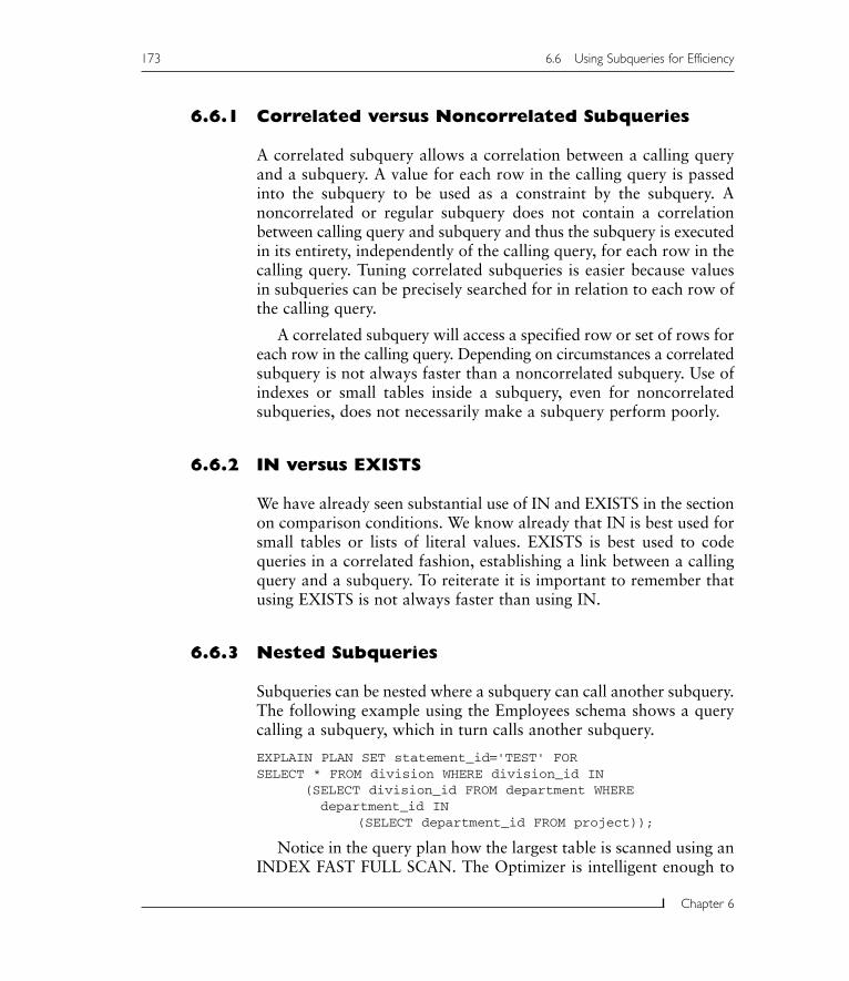
6.6.1 Correlated versus Noncorrelated Subqueries
A correlated subquery allows a correlation between a calling queryand a subquery. A value for each row in the calling query is passedinto the subquery to be used as a constraint by the subquery. Anoncorrelated or regular subquery does not contain a correlationbetween calling query and subquery and thus the subquery is executedin its entirety, independently of the calling query, for each row in thecalling query. Tuning correlated subqueries is easier because valuesin subqueries can be precisely searched for in relation to each row ofthe calling query.
A correlated subquery will access a specified row or set of rows foreach row in the calling query. Depending on circumstances a correlatedsubquery is not always faster than a noncorrelated subquery. Use ofindexes or small tables inside a subquery, even for noncorrelatedsubqueries, does not necessarily make a subquery perform poorly.
6.6.2 IN versus EXISTS
We have already seen substantial use of IN and EXISTS in the sectionon comparison conditions. We know already that IN is best used forsmall tables or lists of literal values. EXISTS is best used to codequeries in a correlated fashion, establishing a link between a callingquery and a subquery. To reiterate it is important to remember thatusing EXISTS is not always faster than using IN.
6.6.3 Nested Subqueries
Subqueries can be nested where a subquery can call another subquery.The following example using the Employees schema shows a querycalling a subquery, which in turn calls another subquery.
EXPLAIN PLAN SET statement_id='TEST' FORSELECT * FROM division WHERE division_id IN
(SELECT division_id FROM department WHEREdepartment_id IN
(SELECT department_id FROM project));
Notice in the query plan how the largest table is scanned using anINDEX FAST FULL SCAN. The Optimizer is intelligent enough to
173 6.6 Using Subqueries for Efficiency
Chapter 6
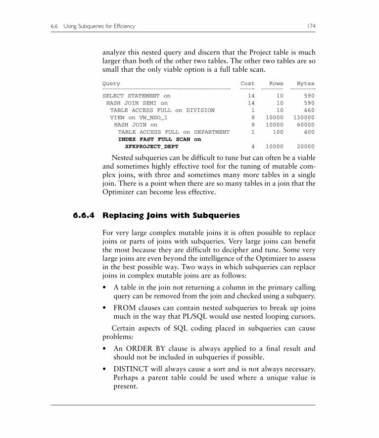
analyze this nested query and discern that the Project table is muchlarger than both of the other two tables. The other two tables are sosmall that the only viable option is a full table scan.
Query Cost Rows Bytes
SELECT STATEMENT on 14 10 590HASH JOIN SEMI on 14 10 590TABLE ACCESS FULL on DIVISION 1 10 460VIEW on VW_NSO_1 8 10000 130000HASH JOIN on 8 10000 60000TABLE ACCESS FULL on DEPARTMENT 1 100 400INDEX FAST FULL SCAN onXFKPROJECT_DEPT 4 10000 20000
Nested subqueries can be difficult to tune but can often be a viableand sometimes highly effective tool for the tuning of mutable com-plex joins, with three and sometimes many more tables in a singlejoin. There is a point when there are so many tables in a join that theOptimizer can become less effective.
6.6.4 Replacing Joins with Subqueries
For very large complex mutable joins it is often possible to replacejoins or parts of joins with subqueries. Very large joins can benefitthe most because they are difficult to decipher and tune. Some verylarge joins are even beyond the intelligence of the Optimizer to assessin the best possible way. Two ways in which subqueries can replacejoins in complex mutable joins are as follows:
• A table in the join not returning a column in the primary callingquery can be removed from the join and checked using a subquery.
• FROM clauses can contain nested subqueries to break up joinsmuch in the way that PL/SQL would use nested looping cursors.
Certain aspects of SQL coding placed in subqueries can causeproblems:
• An ORDER BY clause is always applied to a final result andshould not be included in subqueries if possible.
• DISTINCT will always cause a sort and is not always necessary.Perhaps a parent table could be used where a unique value ispresent.
6.6 Using Subqueries for Efficiency 174

• When testing against subqueries retrieve, filter, and aggregate onindexes not tables. Indexes usually offer better performance.
• Do not be too concerned about full table scans on very smallstatic tables.
� Instances where joins can be replaced with subqueries often involvedatabases with heavy outer join requirements. Excessive use ofSQL outer joins is possibly indicative of an over-granular datamodel structure. However, it could also indicate orphaned childtable rows or the opposite: redundant static data. Cleaning outredundant or orphaned rows can sometimes help performanceimmensely by negating the need for outer joins.
Remove Tables Without Returned ColumnsUsing EXISTS
Going back to the Accounts schema once again look at the followingcomplex mutable join. We are joining four tables and selecting a col-umn from only one of the tables. EXISTS comparisons can be placedinto the WHERE clause to force index access, removing three tablesfrom the join.
EXPLAIN PLAN SET statement_id='TEST' FORSELECT c.nameFROM customer c JOIN orders o USING(customer_id)
JOIN ordersline ol USING(order_id)JOIN transactions t USING(customer_id)
JOIN transactionsline tlUSING(transaction_id)
WHERE c.balance > 0;
Its query plan is a little scary. There are three full table scans andtwo full index scans. The objective is to remove full table scans andchange as many index scans as possible into unique index scans.
Query Cost Rows Bytes
SELECT STATEMENT on ###### ####### #########MERGE JOIN on ###### ####### #########SORT JOIN on ###### ####### #########MERGE JOIN on 4988 ####### #########
175 6.6 Using Subqueries for Efficiency
Chapter 6

SORT JOIN on 3209 100136 3805168HASH JOIN on 762 100136 3805168TABLE ACCESS FULL onCUSTOMER 9 2690 69940
MERGE JOIN on 316 100237 1202844INDEX FULL SCAN onXFK_ORDERLINE_ORDER 26 540827 2704135
SORT JOIN on 290 31935 223545TABLE ACCESS FULL onORDERS 112 31935 223545
SORT JOIN on 1780 188185 1317295TABLE ACCESS FULL onTRANSACTIONS 187 188185 1317295
SORT JOIN on 5033 570175 2850875INDEX FAST FULL SCAN onXFK_TRANSLINE_TRANS 4 570175 2850875
Only the Customer.NAME column is selected. This query is anextreme case but we can actually remove every table from the joinexcept the Customer table. Let’s show this in two stages. Firstly,I will remove the transaction tables from the join.
EXPLAIN PLAN SET statement_id='TEST' FORSELECT c.nameFROM customer c JOIN orders o ON(c.customer_id =o.customer_id)
JOIN ordersline ol USING(order_id)WHERE c.balance > 0AND EXISTS(
SELECT t.transaction_id FROM transactions tWHERE t.customer_id = c.customer_idAND EXISTS(
SELECT transaction_id FROMtransactionsline
WHERE transaction_id = t.transaction_id)
);
We have now reduced the full table scans to two, have a single fullindex scan and most importantly index range scans on both of thetransaction tables.
Query Cost Rows Bytes
SELECT STATEMENT on 359 5007 190266FILTER onHASH JOIN on 359 5007 190266TABLE ACCESS FULL on CUSTOMER 9 135 3510
6.6 Using Subqueries for Efficiency 176

MERGE JOIN on 316 100237 1202844INDEX FULL SCAN onXFK_ORDERLINE_ORDER 26 540827 2704135
SORT JOIN on 290 31935 223545TABLE ACCESS FULL on ORDERS 112 31935 223545
NESTED LOOPS on 72 212 2544TABLE ACCESS BY INDEX ROWID onTRANSACTIONS 2 70 490INDEX RANGE SCAN onXFX_TRANS_CUSTOMER 1 70
INDEX RANGE SCAN onXFK_TRANSLINE_TRANS 1 570175 2850875
Now let’s get completely ridiculous and remove every table fromthe join but the Customer table.
EXPLAIN PLAN SET statement_id='TEST' FORSELECT c.name FROM customer cWHERE c.balance > 0AND EXISTS(
SELECT o.order_id FROM orders oWHERE o.customer_id = c.customer_idAND EXISTS(
SELECT order_id FROM orderslineWHERE order_id = o.order_id
))AND EXISTS(
SELECT t.transaction_id FROM transactions tWHERE t.customer_id = c.customer_idAND EXISTS(
SELECT transaction_id FROMtransactionsline
WHERE transaction_id = t.transaction_id)
);
This is about the best that can be done with this query, now nolonger a join. This final result has full table access on the Customertable only, along with four index range scans. We could possiblyimprove the query further by decreasing the number of Customerrows retrieved using filtering.
Query Cost Rows Bytes
SELECT STATEMENT on 9 7 182FILTER onTABLE ACCESS FULL on CUSTOMER 9 7 182
177 6.6 Using Subqueries for Efficiency
Chapter 6
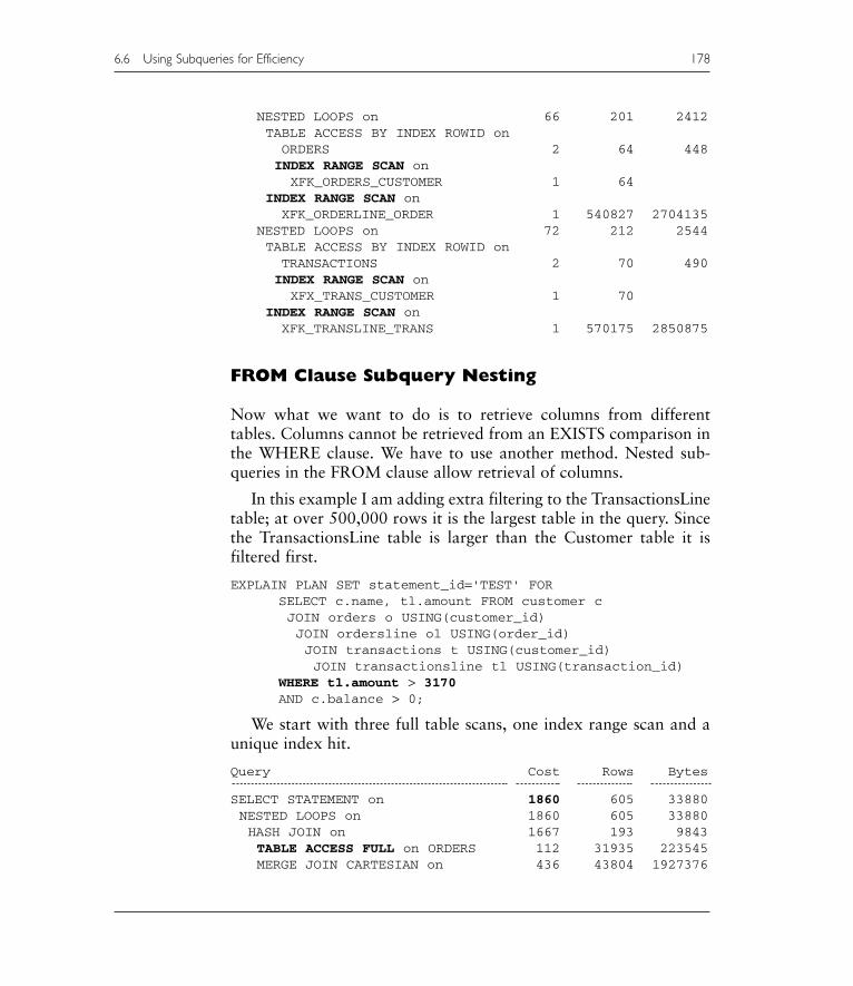
NESTED LOOPS on 66 201 2412TABLE ACCESS BY INDEX ROWID onORDERS 2 64 448INDEX RANGE SCAN onXFK_ORDERS_CUSTOMER 1 64
INDEX RANGE SCAN onXFK_ORDERLINE_ORDER 1 540827 2704135
NESTED LOOPS on 72 212 2544TABLE ACCESS BY INDEX ROWID onTRANSACTIONS 2 70 490INDEX RANGE SCAN onXFX_TRANS_CUSTOMER 1 70
INDEX RANGE SCAN onXFK_TRANSLINE_TRANS 1 570175 2850875
FROM Clause Subquery Nesting
Now what we want to do is to retrieve columns from differenttables. Columns cannot be retrieved from an EXISTS comparison inthe WHERE clause. We have to use another method. Nested sub-queries in the FROM clause allow retrieval of columns.
In this example I am adding extra filtering to the TransactionsLinetable; at over 500,000 rows it is the largest table in the query. Sincethe TransactionsLine table is larger than the Customer table it isfiltered first.
EXPLAIN PLAN SET statement_id='TEST' FORSELECT c.name, tl.amount FROM customer cJOIN orders o USING(customer_id)JOIN ordersline ol USING(order_id)JOIN transactions t USING(customer_id)JOIN transactionsline tl USING(transaction_id)
WHERE tl.amount > 3170AND c.balance > 0;
We start with three full table scans, one index range scan and aunique index hit.
Query Cost Rows Bytes
SELECT STATEMENT on 1860 605 33880NESTED LOOPS on 1860 605 33880HASH JOIN on 1667 193 9843TABLE ACCESS FULL on ORDERS 112 31935 223545MERGE JOIN CARTESIAN on 436 43804 1927376
6.6 Using Subqueries for Efficiency 178

NESTED LOOPS on 292 16 288TABLE ACCESS FULL onTRANSACTIONSLINE 276 16 176
TABLE ACCESS BY INDEX ROWID onTRANSACTIO 1 188185 1317295INDEX UNIQUE SCAN onXPKTRANSACTIONS 188185
BUFFER SORT on 435 2690 69940TABLE ACCESS FULL on CUSTOMER 9 2690 69940
INDEX RANGE SCAN onXFK_ORDERLINE_ORDER 1 540827 2704135
Firstly, some appropriate simple tuning can be done. Since theTransactionsLine table is the largest table with the smallest relativefiltered result, it should be selected from first.
� The first table to be processed should be the largest table with thelargest relative row reduction filter. In other words, the biggesttable with the lowest number of rows retrieved from it. This appliesto both the FROM clause and the WHERE clause. Always reducerows to be joined first.
EXPLAIN PLAN SET statement_id='TEST' FORSELECT c.name, tl.amount FROM transactionsline tlJOIN transactions t USING(transaction_id)JOIN customer c USING(customer_id)JOIN orders o USING(customer_id)JOIN ordersline ol ON(ol.order_id = o.order_id)
WHERE tl.amount > 3170AND c.balance > 0;
Appropriate simple tuning yields one full table scan, two indexrange scans, and two unique index hits.
Query Cost Rows Bytes
SELECT STATEMENT on 1381 3267 182952NESTED LOOPS on 1381 3267 182952NESTED LOOPS on 340 1041 53091NESTED LOOPS on 308 16 704NESTED LOOPS on 292 16 288TABLE ACCESS FULL onTRANSACTIONSLINE 276 16 176
TABLE ACCESS BY INDEX ROWIDon TRANSACTIO 1 33142 231994
179 6.6 Using Subqueries for Efficiency
Chapter 6

INDEX UNIQUE SCAN onXPKTRANSACTIONS 33142
TABLE ACCESS BY INDEX ROWID onCUSTOMER 1 2690 69940INDEX UNIQUE SCAN onXPKCUSTOMER 2690
TABLE ACCESS BY INDEX ROWID onORDERS 2 172304 1206128INDEX RANGE SCAN onXFK_ORDERS_CUSTOMER 1 172304
INDEX RANGE SCAN onXFK_ORDERLINE_ORDER 1 540827 2704135
Now let’s use the FROM clause to create nested subqueries.The trick is to put the largest table with the most severe filter at thedeepest nested level, forcing it to execute first. Thus we start with theTransactionsLine table.
EXPLAIN PLAN SET statement_id='TEST' FORSELECT c.name, b.amountFROM customer c,(
SELECT t.customer_id, a.amountFROM transactions t,(
SELECT transaction_id, amount FROMtransactionsline
WHERE amount > 3170) aWHERE t.transaction_id = a.transaction_id
) b, orders o, ordersline olWHERE c.balance > 0AND c.customer_id = b.customer_idAND o.customer_id = c.customer_idAND ol.order_id = o.order_id;
The cost is reduced further with the same combination of scansbecause fewer rows are being joined.
Query Cost Rows Bytes
SELECT STATEMENT on 533 605 33880NESTED LOOPS on 533 605 33880NESTED LOOPS on 340 193 9843NESTED LOOPS on 308 16 704NESTED LOOPS on 292 16 288TABLE ACCESS FULL onTRANSACTIONSLINE 276 16 176
6.6 Using Subqueries for Efficiency 180

TABLE ACCESS BY INDEX ROWID on TRANSACTIO 1 33142 231994INDEX UNIQUE SCAN onXPKTRANSACTIONS 33142
TABLE ACCESS BY INDEX ROWID on CUSTOMER 1 2690 69940INDEX UNIQUE SCAN onXPKCUSTOMER 2690
TABLE ACCESS BY INDEX ROWID onORDERS 2 31935 223545INDEX RANGE SCAN onXFK_ORDERS_CUSTOMER 1 31935
INDEX RANGE SCAN onXFK_ORDERLINE_ORDER 1 540827 2704135
Now let’s combine WHERE clause comparison subqueries andFROM clause embedded subqueries.
EXPLAIN PLAN SET statement_id='TEST' FORSELECT c.name, b.amountFROM customer c,(
SELECT t.customer_id, a.amountFROM transactions t,(
SELECT transaction_id, amount FROMtransactionsline
WHERE amount > 3170) aWHERE t.transaction_id = a.transaction_id
) bWHERE c.balance > 0AND EXISTS(
SELECT o.order_id FROM orders oWHERE o.customer_id = c.customer_idAND EXISTS(
SELECT order_id FROM orderslineWHERE order_id = o.order_id
));
Using EXISTS makes the query just that little bit faster with lowercost since the number of tables joined is reduced.
Query Cost Rows Bytes
SELECT STATEMENT on 420 2190 91980FILTER onNESTED LOOPS on 420 2190 91980
181 6.6 Using Subqueries for Efficiency
Chapter 6

MERGE JOIN CARTESIAN on 420 2190 81030TABLE ACCESS FULL onTRANSACTIONSLINE 276 16 176
BUFFER SORT on 144 135 3510TABLE ACCESS FULL on CUSTOMER 9 135 3510
INDEX UNIQUE SCAN onXPKTRANSACTIONS 188185 940925
NESTED LOOPS on 66 201 2412TABLE ACCESS BY INDEX ROWID onORDERS 2 64 448INDEX RANGE SCAN onXFK_ORDERS_CUSTOMER 1 64
INDEX RANGE SCAN onXFK_ORDERLINE_ORDER 1 540827 2704135
6.7 Using Synonyms
A synonym is, as its name implies, another name for a known object.Synonyms are typically used to reference tables between schemas.Public synonyms make tables contained within schemas available toall schemas. Apart from the obvious security issues there can bepotential performance problems when over-using synonyms in highlyconcurrent environments. It may not necessarily be effective to dividefunctionality between different schemas only to allow users global orsemi-global access to all of the underlying schemas. Simplicity indevelopment using objects like synonyms often leads to complexityand performance problems in production. Additionally too manymetadata objects can cause problems with the shared pool.
6.8 Using Views
Views are application- and security-friendly. Views can also be usedto reduce complexity, particularly in development. In general, viewsare not conducive to good performance. A view is a logical overlay ontop of one or more tables. A view is created using an SQL statement.A view does not contain data itself. The biggest problem with a view isthat whenever it is queried its defining SQL statement is re-executed.It is common in applications for a developer to query a view and addadditional filtering. The potential results are views containing largequeries where programmers will then execute small row number
6.8 Using Views 182

retrievals from the view. Thus two queries are executed, commonlywith the view query selecting all the rows in the underlying tableor join.
Let’s try to prove that views are inherently slower than directtable queries. Firstly, I create a view on my largest Accounts schematable.
CREATE VIEW glv AS SELECT * FROM generalledger;
Now let’s do some query plans. I have four queries and query planslisted. The first two retrieve a large number of rows from the view andthen the table. It is apparent that the query plans are identical in cost.
Selecting from the view:
EXPLAIN PLAN SET statement_id='TEST' FORSELECT * FROM glv WHERE coa# = '40003';
Query Cost Rows Bytes
SELECT STATEMENT on 165 150548 3914248TABLE ACCESS BY INDEX ROWID onGENERALLEDGE 165 150548 3914248INDEX RANGE SCAN on XFK_GL_COA# 5 150548
Selecting from the table:
EXPLAIN PLAN SET statement_id='TEST' FORSELECT * FROM generalledger WHERE coa# = '40003';
Query Cost Rows Bytes
SELECT STATEMENT on 165 150548 3914248TABLE ACCESS BY INDEX ROWID onGENERALLEDGE 165 150548 3914248INDEX RANGE SCAN on XFK_GL_COA# 5 150548
Now let’s filter and return much fewer rows. Once again thequery plans are the same.
Selecting from the view:
EXPLAIN PLAN SET statement_id='TEST' FORSELECT * FROM glv WHERE generalledger_id = 500000;
Query Cost Rows Bytes
SELECT STATEMENT on 3 1 26TABLE ACCESS BY INDEX ROWID onGENERALLEDGE 3 1 26INDEX UNIQUE SCAN on XPKGENERALLEDGER 2 1
183 6.8 Using Views
Chapter 6

Selecting from the table:
EXPLAIN PLAN SET statement_id='TEST' FORSELECT * FROM generalledger WHERE generalledger_id =500000;
Query Cost Rows Bytes
SELECT STATEMENT on 3 1 26TABLE ACCESS BY INDEX ROWID onGENERALLEDGE 3 1 26INDEX UNIQUE SCAN on XPKGENERALLEDGER 2 1
So let’s now try some time tests. The COUNT function is used asa wrapper and each query is executed twice to ensure there is no con-flict between reading from disk and memory.
SELECT COUNT(*) FROM(SELECT * FROM glv WHERE coa# = '40003');SELECT COUNT(*) FROM(SELECT * FROM generalledger WHEREcoa# = '40003');
SELECT COUNT(*) FROM(SELECT * FROM glvWHERE generalledger_id = 500000);
SELECT COUNT(*) FROM(SELECT * FROM generalledgerWHERE generalledger_id = 500000);
In the first two instances retrieving from the view is faster thanreading from the table.
SQL> SELECT COUNT(*) FROM(SELECT * FROM glv WHEREcoa# = '40003');
COUNT(*)
66287
Elapsed: 00:00:04.04
SQL> SELECT COUNT(*) FROM(SELECT * FROM generalledger WHEREcoa# = '40003');
COUNT(*)
66287
Elapsed: 00:00:04.09
SQL> SELECT COUNT(*) FROM(SELECT * FROM glv WHEREgeneralledger_id = 500000);
COUNT(*)
1
6.8 Using Views 184

Elapsed: 00:00:00.00
SQL> SELECT COUNT(*) FROM(SELECT * FROM generalledger WHEREgeneralledger_id = 500000);
COUNT(*)
1
Elapsed: 00:00:00.00
For a single table and a view on that table there is no differencein query plan or execution time.
Now let’s go and re-create our view and re-create it with a joinrather than just a single table. This code drops and re-creates theview I created previously.
DROP VIEW glv;CREATE VIEW glv AS
SELECT gl.generalledger_id, coa.coa#, t.text AS type,st.text AS subtype, coa.text as coa, gl.dr,gl.cr, gl.dte
FROM type t JOIN coa USING(type)JOIN subtype st USING(subtype)
JOIN generalledger gl ON(gl.coa# =coa.coa#);
When retrieving a large percentage of rows in the following twoqueries the cost in the query plan is much better when retrievingusing the tables join rather than the view.
Selecting from the view:
EXPLAIN PLAN SET statement_id='TEST' FORSELECT * FROM glv WHERE coa# = '40003';
Query Cost Rows Bytes
SELECT STATEMENT on 168 30110 2107700NESTED LOOPS on 168 30110 2107700NESTED LOOPS on 3 1 44NESTED LOOPS on 2 1 34TABLE ACCESS BY INDEX ROWID on COA 1 1 25INDEX UNIQUE SCAN on XPKCOA 1
TABLE ACCESS BY INDEX ROWID onTYPE 1 6 54INDEX UNIQUE SCAN on XPKTYPE 6
TABLE ACCESS BY INDEX ROWID onSUBTYPE 1 4 40
185 6.8 Using Views
Chapter 6

INDEX UNIQUE SCAN on XPKSUBTYPE 4TABLE ACCESS BY INDEX ROWID onGENERALLEDG 165 150548 3914248INDEX RANGE SCAN on XFK_GL_COA# 5 150548
Selecting from the table join:
EXPLAIN PLAN SET statement_id='TEST' FORSELECT gl.generalledger_id, coa.coa#, t.text AS type,
st.text AS subtype, coa.text as coa, gl.dr,gl.cr, gl.dte
FROM type t JOIN coa USING(type)JOIN subtype st USING(subtype)
JOIN generalledger gl ON(gl.coa# =coa.coa#)
WHERE gl.coa# = '40003';
Query Cost Rows Bytes
SELECT STATEMENT on 5 30110 2107700NESTED LOOPS on 5 30110 2107700NESTED LOOPS on 3 1 44NESTED LOOPS on 2 1 34TABLE ACCESS BY INDEX ROWID on COA 1 1 25INDEX UNIQUE SCAN on XPKCOA 1
TABLE ACCESS BY INDEX ROWID on TYPE 1 6 54INDEX UNIQUE SCAN on XPKTYPE 6
TABLE ACCESS BY INDEX ROWID on SUBTYPE 1 4 40INDEX UNIQUE SCAN on XPKSUBTYPE 4
TABLE ACCESS BY INDEX ROWID onGENERALLEDG 2 150548 3914248INDEX RANGE SCAN on XFK_GL_COA# 1 150548
Let’s try some timing tests. The first timing test retrieves a largeset of rows from the view.
SQL> SELECT COUNT(*) FROM(SELECT * FROM glv WHERE coa# ='40003');
COUNT(*)
66287
Elapsed: 00:00:04.02
The second timing test retrieves the same large set of rows fromthe table join and is obviously much faster.
6.8 Using Views 186

SQL> SELECT COUNT(*) FROM(2 SELECT gl.generalledger_id, coa.coa#, t.text AS type,
st.text AS subtype, coa.text as coa, gl.dr, gl.cr,gl.dte
3 FROM type t JOIN coa USING(type)4 JOIN subtype st USING(subtype)5 JOIN generalledger gl ON(gl.coa# = coa.coa#)6 WHERE gl.coa# = '40003');
COUNT(*)
66287
Elapsed: 00:00:00.07
Comparing times to retrieve a single row, there is no differencebetween the view and the retrieval from the join. In a highly activeconcurrent environment this would probably not be the case.
SQL> SELECT COUNT(*) FROM(SELECT * FROM glv WHEREgeneralledger_id = 500000);
COUNT(*)
1
Elapsed: 00:00:00.00
SQL> SELECT COUNT(*) FROM (SELECT gl.generalledger_id,coa.coa#, t.text
AS type, st.text AS subtype, coa.text as coa, gl.dr, gl.cr,gl.dte
2 FROM generalledger gl JOIN coa ON(gl.coa# = coa.coa#)3 JOIN type t USING(type)4 JOIN subtype st USING(subtype)5 WHERE generalledger_id = 500000);
COUNT(*)
1
Elapsed: 00:00:00.00
Views can now have constraints, including primary and foreignkey constraints. These may help performance of data retrieval fromviews. However, assuming that views are created for coding devel-opment simplicity and not security, adding complexity to a viewwould negate the simplification issue.
The exception to views re-executing every time they are queriedis a Materialized View. A Materialized View is a separate database
187 6.8 Using Views
Chapter 6

object in Oracle Database and stores the results of a query. Thuswhen a Materialized View is queried, data is extracted from the viewand not the underlying objects in the query. Materialized Views areread only and intended for use in data warehousing and replication.
Views are not performance friendly! For the sake of performancedo not use views. Some applications are built with multiple layers ofviews. This type of application design is often application convenientand can produce disappointing results with respect to databaseperformance. There is simply too much metadata in the shared pool.A brute force method of resolving selection of rows from multiplelayered sets of views is to use a form of the FROM clause in theSELECT statement with the ONLY clause included as shown in thefollowing syntax. The ONLY clause will not retrieve rows fromsubset views.
SELECT … FROM ONLY (query) …
6.9 Temporary Tables
In years past in traditional relational databases temporary tableswere created as shell structures to contain temporarily generateddata, usually for the purposes of reporting. Oracle Database has theability to create tables containing temporary rows. Rows created intemporary table objects are created locally to a session, somewhatmanaged by the database. It is more efficient to use Oracle Databasetemporary table objects in some circumstances. Creating traditionaltemporary tables, filling them, emptying them, and storing or delet-ing their rows is unlikely to perform better than Oracle Databasetemporary table objects.
6.10 Resorting to PL/SQL
PL/SQL is an acronym for Programming Language for SQL. From apurely programming perspective PL/SQL is really SQL with program-ming logic wrapper controls, amongst numerous other bells andwhistles. PL/SQL is a very primitive programming language at best.Beware of writing entire applications using PL/SQL. SQL is designedto retrieve sets of data from larger sets and is not procedural, sequential,
6.10 Resorting to PL/SQL 188
or object-like in nature. Programming languages are required to beone of those or a combination thereof. PL/SQL has its place as a rela-tional database access language and not as a programming language.Additionally PL/SQL is interpretive which means it is slow!
PL/SQL objects are now stored in compiled form in binaryobject variables or BLOB objects. This helps PL/SQL procedureexecution performance.
Does PL/SQL allow for faster performance? The short answer is no.The long answer is as follows. PL/SQL allows much greater controlover SQL coding than simple SQL does. However, modern OracleSQL is much more sophisticated than it was years ago and some ofthe aspects of PL/SQL used in the past allowing better performancein PL/SQL than SQL are effectively redundant, particularly withretrieval of data.
There are a number of reasons for resorting to PL/SQL:
• PL/SQL will not provide better performance but will allow a break-down of complexity. Breaking down complexity can allow easiertuning of SQL statements through better control of cursors.
• An obvious benefit of PL/SQL is the ability to build stored proce-dures and triggers. Triggers should be used sparingly and avoidedfor implementation of Referential Integrity; constraints are muchfaster. In the case of stored procedures the obvious benefits arecentralized control and potential performance increases becausestored procedure code is executed on the server. Execution on adatabase server reduces network traffic.
• There are some situations where it is impossible to code SQL codeusing SQL alone and thus PL/SQL has to be resorted to. As OracleCorporation has developed SQL this has become less frequent.
• Some exceedingly complex SQL code can benefit from the use ofPL/SQL instead of SQL. Some SQL code can become so complexthat it is impossible to tune or even code in SQL and hencePL/SQL becomes the faster option. Using the DECODE functionis similar to control structures such as IF and CASE statements.PL/SQL allows all the appropriate control structures.
• PL/SQL packages can be cached into memory to avoid re-parsing.
189 6.10 Resorting to PL/SQL
Chapter 6
10g

PL/SQL can provide better program coding control of cursorsplus execution and maintenance from a central, single point. Perhapsthe most significant benefit of resorting to PL/SQL is a potentialreduction in complexity. Once again, as with views, reducing com-plexity is not necessarily conducive to performance tuning. In factsimplicity, as with over-Normalization can often hurt performance ina relational database. Thus further discussion of tuning SQLretrieval code using PL/SQL is largely irrelevant.
Tuning PL/SQL is a programming task and has little to do withcoding well-performing SQL code. The obvious programming pointsto note are as follows:
• Do not process more in a loop or a cursor than is necessary.Break out of loops when no more processing is required.
• Large IF statements should be replaced with CASE statements orappropriate breaks should be used. Traditionally CASE state-ments are faster than IF statements.
• Recursion using embedded procedures creates very elegant codebut in PL/SQL can cause performance problems, especially wheretransactions are not completed. PL/SQL is not executed as com-piled code in the sense that compiled C code is. PL/SQL compi-lation involves syntax parsing and interpretation; no binary copyis created. When PL/SQL code is executed it is interpreted andnot executed from a compiled binary form.
PL/SQL objects are now stored in compiled form in binaryobject variables or BLOB objects. This helps PL/SQL procedureexecution performance.
• The WHERE CURRENT OF clause can refer to a cursor ROWID,giving direct pointer access to a cursor row in memory. TheRETURNING INTO clause can help with reducing the need forsubsequent SELECT statements further on in a procedure byreturning values into variables.
• Explicit cursors can be faster than implicit cursors but are moredifficult to code.
• PL/SQL has three parameter formats for passing variables inand out of procedures. IN and OUT pass values in and out of
6.10 Resorting to PL/SQL 190
10g

procedures, respectively. IN OUT passes a pointer both in andout of a procedure. Use only what is needed.
• As with SQL code embedded in applications, PL/SQL proceduresof any kind can use bind variables. Using bind variables can havea profound effect on increasing performance by lowering parsingrequirements in the library cache.
6.10.1 Tuning DML in PL/SQL
There are two interesting points to note in relation to performanceof DML statements in PL/SQL. Other than what has already beencovered in this chapter there is little else which can be done to tuneDML (INSERT, UPDATE, DELETE, MERGE) or SELECT statementsin PL/SQL.
The RETURNING INTO Clause
In the following example the RETURNING clause prevents the coderhaving to code an extra SELECT statement to find the identifier valuerequired for the second INSERT statement. The same applies simi-larly to the second INSERT statement returning a second value forthe DBMS_OUTPUT.PUT_LINE procedure.
DECLAREdivision_id division.division_id%TYPE;division_name division.name%TYPE;department_name department.name%TYPE;
BEGININSERT INTO division(division_id, name)VALUES(division_seq.NEXTVAL, 'A New Division')RETURNING division_id, name INTO division_id,division_name;
INSERT INTO department(department_id, division_id, name)VALUES(department_seq.NEXTVAL, division_id, 'A NewDepartment')
RETURNING name INTO department_name;
DBMS_OUTPUT.PUT_LINE('Added : '||division_name||', '||department_name);
END;/
191 6.10 Resorting to PL/SQL
Chapter 6

The RETURNING clause can be used to return collections.
6.10.2 When to Resort to PL/SQL and Cursors
In general, SQL in Oracle Database is now powerful enough to dealwith almost any requirement. Some occasions do call for substitutingSQL code nested loop type queries with PL/SQL. PL/SQL providesbetter programming control and allows much easier managementof highly complex SQL code. It is sometimes the case that betterperformance will be gained using PL/SQL to control nested SQLstatements.
PL/SQL can sometimes be faster when compiled, pinned, andexecuted on the database server, depending on the application. Thegoal of stored procedures is to minimize on network traffic. With thespeed of modern network connections available this is not necessar-ily an issue anymore.
So what do I mean by resorting to PL/SQL and cursors? After allI did not just state “Resorting to PL/SQL”. So what am I talkingabout? Look at this example.
EXPLAIN PLAN SET statement_id='TEST' FORSELECT * FROM coa NATURAL JOIN generalledger;
This query plan shows the COA table in the outer loop and theGeneralLedger table in the inner loop.
Query Cost Rows Bytes
1. SELECT STATEMENT on 1642 1068929 502396632. HASH JOIN on 1642 1068929 502396633. TABLE ACCESS FULL on COA 2 55 13203. TABLE ACCESS FULL on
GENERALLEDGER 1128 1068929 24585367
To convert the SQL statement shown previously to PL/SQLI would need PL/SQL code something similar to that shown here.
DECLARECURSOR cCOA IS SELECT * FROM coa;TYPE tGL IS REF CURSOR RETURN generalledger%ROWTYPE;cGLs tGL;rGL generalledger%ROWTYPE;
6.10 Resorting to PL/SQL 192
10g
BEGINFOR rCOA IN cCOA LOOP
OPEN cGLs FOR SELECT * FROM generalledger WHEREcoa# = rCOA.coa#;
LOOPFETCH cGLs INTO rGL;EXIT WHEN cGLs%NOTFOUND;DBMS_OUTPUT.PUT_LINE(
rCOA.coa#||' '||TO_CHAR(rGL.dte)||' '||TO_CHAR(rGL.dr)||' '||TO_CHAR(rGL.cr));
END LOOP;CLOSE cGLs;
END LOOP;EXCEPTION WHEN OTHERS THEN CLOSE cGLs;END;/
In general, PL/SQL should only replace SQL when coding simplycannot be achieved in SQL, it is too complex and convoluted forSQL, or centralization on the database server is required.
6.10.3 Java or PL/SQL?
Java can be used to construct stored procedures in much the sameway that PL/SQL can. When to use Java? That is a question with avery simple answer. Use Java when not accessing the database andwriting code which is computationally heavy. What does this mean?When answering a question such as this I always prefer to go backinto the roots of a programming language or a database. In otherwords, what were PL/SQL and Java originally built for? What istheir purpose? Let’s start by looking at PL/SQL.
PL/SQL is effectively a primitive programming language and ispurely an extension of SQL. SQL was originally built purely for thepurpose of accessing data in a relational database. Therefore, it fol-lows that PL/SQL is of the same ilk as SQL. PL/SQL was originallydevised to create stored procedures in Oracle Database. Stored pro-cedures were devised for relational databases in general, not justOracle Database, to allow for coding of self-contained blocks oftransaction-based SQL code. Those blocks of code are executed onthe database server thus minimizing on network traffic. PL/SQL is
193 6.10 Resorting to PL/SQL
Chapter 6

much richer than stored procedure languages used in other relationaldatabases. PL/SQL can be used to code complexity. This takes usto Java.
Why use Java? Java is an object-oriented programming languagebuilt for coding of highly complex front-end and back-end applica-tions. If you know anything about objects at all you will understandthat objects in programming are superb at handling complexity.It is in the very nature of objects to handle complexity by breakingeverything down into its most simplistic parts. Java can be used tohandle highly complex coding sequences and can be used to createOracle Database stored procedures, much in the same way thatPL/SQL can. Java is much more powerful than PL/SQL in doinglots of computations. Java is better than PL/SQL at anything thatdoes not involve accessing the database, especially complex code.Coding requirements when accessing a database are trivial in rela-tion to the complex routines and functions required by applications-level coding.
There is one small but fairly common problem with using Java.Java is object oriented. Oracle Database is relational. Object andrelational methodologies do not mix well. Many Java applications, dueto their object nature, break things into very small, easily manageablepieces. Object-oriented design is all about easy management of com-plexity. In relational terms management of complexity by severebreak-down and object “black boxing” is an incredible level ofNormalization. Too much Normalization leads to too much granu-larity and usually very slow performance. What commonly happenswith Java applications is one or all of a number of things. These aresome of the possibilities.
• Pre-loading of large data sets.
• Separation of parts of SQL statements into separate commandssent to the database. For instance, a SELECT statement could besubmitted and then filtering would be performed in the Javaapplication itself. This leads to lots of full table scans and aplethora of other performance problems.
• Sometimes object design is imposed onto the database to suchan extent as to continually connect to and disconnect from thedatabase for every SQL code execution. This is very heavy ondatabase resource consumption.
6.10 Resorting to PL/SQL 194

So what’s the answer to the nagging question of using Java orPL/SQL? The answer is to use both, if your skills set permits it. Javacan be used to handle any kind of complex code not accessing thedatabase. PL/SQL should be used to access the database. If you can-not or do not wish to use a mix and prefer Java then be aware thata relational database is not able to manage the complete and total“black box” breakdown into easily definable and understandableindividual objects. Do not attempt to impose an object structure ona relational or furthermore even an object-relational database: theyare not designed for that level of granularity.
6.11 Replacing DELETE with TRUNCATE
The DDL TRUNCATE command is faster than using the DELETEcommand when deleting all the rows from a table. The TRUNCATEcommand automatically commits and does not create any log entriesor rollback. The obvious problem with TRUNCATE is that an errorcannot be undone.
6.12 Object and Relational Conflicts
Relational and object data model structures are completely differentto each other. There is great potential for conflict when combiningthese two methodologies into what is called an object-relationaldatabase. These conflicts can hamper performance in a relationaldatabase such as Oracle Database.
6.12.1 Large Binary Objects in a Relational Database
The biggest benefit to the combination of objects and relations isthat of including large binary objects into a relational structure, suchas multimedia objects. However, there is a twist. In both relationaland object databases the most efficient storage method for multime-dia objects is to use a BFILENAME pointer. A BFILENAME pointerdoes not store the object itself in the database but contains a path andfile name for the object. The object is stored externally to the data-base in the file system. Storing large binary objects in any database
195 6.12 Object and Relational Conflicts
Chapter 6

is inefficient because those binary objects can span multiple blocks,both Oracle Database blocks and operating system blocks. Even withOracle9i Database multiple block sizes and specific storage structuresfor LOB datatypes large multimedia objects will span more than oneblock. Storing data into a database which spans more than a single blockis effectively row chaining where a row is “chained” from one block toanother. Chaining is not really an issue if the blocks are physically nextto each other. Also the DB_FILE_MULTIBLOCK_READ_COUNTparameter can help to counteract this. The fact is contiguous, defrag-mented block storage is extremely unlikely in any database environment.It is usually best to store large singular binary objects in the file system.
BIGFILE tablespaces can possibly help to alleviate these issuessomewhat.
6.12.2 Object-Relational Collections
Including TABLE and VARRAY collections inside relational tablesand within PL/SQL is generally a very bad idea. Collections are anobject methodological approach to object data abstraction andencapsulation. Object methodologies are completely opposed tothose of relational databases. An object structure is spherical allow-ing access from any point to any point within an entire database. Arelational database is more two-dimensional in nature and requiresthat access to data be passed through or down semi-hierarchicalstructures or into subset parts of a data model. Since PL/SQL ismerely an extension of SQL, and SQL is a purely relational databaseaccess language, any type of object coding is best avoided usingPL/SQL. If you want to write object code use Java. Java is built forobject structures.
The same approach applies to including object structures in tables.There are various instances in which collection substructures can beutilized in relational database tables. 1st Normal Form master detailand 2nd Normal Form foreign key static table inclusion relation-ships are possibilities. However, storage structures remain applicableto a relational methodology and are still ultimately stored in rows(tuples). Tables and rows are two-dimensional. Object structures are
6.12 Object and Relational Conflicts 196
10g

multi-dimensional. The two do not fit together. If you must containcollections in tables in Oracle Database there are various objectcollection types that could be used. Associative arrays are the mostefficient.
• Nested Table. A nested table is a dynamic array. A dynamic arrayis a pointer. A pointer does not require a specific size limit andthus the use of the term dynamic. Dynamic implies that it canhave any number of rows or entries in its array.
• VARRAY. A VARRAY is a fixed-length array. A fixed-lengtharray is a reserved chunk of memory saved for multiple arrayrows. Unlike a dynamic array a fixed-length array has space inmemory reserved for the whole array structure.
• Associative Array. An associative array is an indexed dynamicarray and can potentially be accessed faster than a nested tablebecause it can be accessed using an index.
Problems with objects in relational models are more often thannot a misunderstanding of object-modeling techniques. It is commonknowledge that the approach required for object data modeling iscompletely different to that of relational modeling. The same is verylikely to apply to object-relational modeling using object types suchas nested table, VARRAY or associative array collections in OracleDatabase tables. Using these collection data types requires object andrelational modeling skills, not only relational modeling skills.
That ends this chapter on examining the basics of how to createefficient SQL. In the next chapter we will look at indexing and startto delve a little deeper into Oracle Database specifics.
197 6.12 Object and Relational Conflicts
Chapter 6

625
21Tools and Utilities
There are a multitude of tools available to both monitor and tuneOracle installations. This chapter will simply introduce some ofthose tools and categorize what each can do. It is best to explainsome of the various tools graphically. Let’s begin with OracleEnterprise Manager. In Chapter 10 of Part II we looked at the SQLcode tuning aspects of Oracle Enterprise Manager; this chapterattempts to focus on the physical tuning aspects.
21.1 Oracle Enterprise Manager
Oracle Enterprise Manager in relation to physical tuning can bedivided into two parts. These two parts contain diagnostic and tun-ing tools. Diagnosis usually implies monitoring for potential prob-lems and sometimes repairing them; tuning and analysis can evenautomatically repair possible performance problems.
21.1.1 Diagnostics Pack
With respect to physical tuning the interesting parts of the diagnos-tics pack are as follows:
• Event Monitoring. Allows definition, automated detection ofand potential automated “FixIt” jobs, which can automaticallycorrect problems.
• Lock Monitoring. Allows monitoring and resolution of locksin a database.

• TopSessions. Detects and displays the top best- or worst-performingsessions ordered by a large number of different possible sortingparameters.
• TopSQL. Detects and displays the top best- and worst-performingSQL statements, again ordered by a large number of differentpossible sorting parameters.
• Performance Manager. Performance Manager wraps everythingtogether such as details contained in the TopSessions andTopSQL tools, with extra functionality and GUI usability.
� The ultimate of Oracle Enterprise Manager is a GUI windowinterface into the Oracle Database Wait Event Interface.
Event Monitoring
Event monitoring covers areas such as performance, resource usage,how space is used, amongst many other areas. There are an absoluteof plethora of events which can be included for automated detectionand potential “FixIt” action to resolve problems. Figure 21.1 showsa very small subsection of the fully user definable event detectiontool. The event detection construction tool is accessible from theEvent menu in the Oracle Enterprise Manager Console.
Oracle Enterprise Manager repository, events and jobs are auto-matically configured.
Lock Monitoring
Figure 21.2 shows lists of locks on a very busy database. Note thedrilldown menu with various options including the option to kill offa session. Sometimes it is necessary to kill a session causing poten-tially damaging problems.
TopSessions
The TopSessions tool allows ordered visualization of statisticalperformance information where the best or worst sessions can be
21.1 Oracle Enterprise Manager 626
10g

displayed first. Figure 21.3 shows the first 10 sessions executing themost physical reads.
TopSQL
TopSQL is similar to the TopSessions tool where the TopSQL tooldetects and displays the best- or worst-performing SQL statements ina large number of different possible orders. An example of TopSQLis shown in Figure 21.4.
TopSQL is much improved in relation to more usable reportingcapabilities.
627 21.1 Oracle Enterprise Manager
Chapter 21
Figure 21.1 Defining Events for Detection and Resolution
10g

Performance Manager
The Performance Manager is a very comprehensive tool. It allowsan intensive GUI picture of an environment with every possiblemonitoring and performance metric imaginable. The PerformanceManager appears complex but it is comprehensive and very easilyusable.
Figure 21.5 shows the Performance Overview screen. This screenis accessible from the Oracle Enterprise Manager Console on theTools menu. Select the Diagnostic Pack submenu. The PerformanceOverview interface gives an overall picture of database performance
21.1 Oracle Enterprise Manager 628
Figure 21.2 Monitoring and Managing Locking

and is highly adaptable depending on requirements and what youwant to monitor.
Performance Overview charts are much improved allowingmonitoring and diagnostics checking from a central point usingan HTML interface.
The Performance Manager allows simple drill-down furtherinto the separate subset areas of those shown in PerformanceOverview interface, to the point and beyond of drilling down
629 21.1 Oracle Enterprise Manager
Chapter 21
Figure 21.3 TopSessions Monitoring in a Specified Order
10g
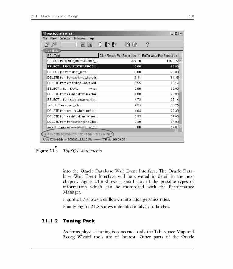
into the Oracle Database Wait Event Interface. The Oracle Data-base Wait Event Interface will be covered in detail in the nextchapter. Figure 21.6 shows a small part of the possible types ofinformation which can be monitored with the PerformanceManager.
Figure 21.7 shows a drilldown into latch get/miss rates.
Finally Figure 21.8 shows a detailed analysis of latches.
21.1.2 Tuning Pack
As far as physical tuning is concerned only the Tablespace Map andReorg Wizard tools are of interest. Other parts of the Oracle
21.1 Oracle Enterprise Manager 630
Figure 21.4 TopSQL Statements

Enterprise Manager tuning pack were covered in Chapter 10 of Part IIof this book.
Tablespace Map and the Reorg Wizard
The tablespace map presents a graphical representation of physicaldata distribution within tablespaces. After executing a tablespaceanalysis in the INDX tablespace of my database, two indexes arerecommended for reorganization, as shown in Figure 21.9.
As can be seen in the drop-down menu in Figure 21.9 variousoptions are available:
• Tablespace Analysis. Analyze a tablespace for problems such asfragmentation.
• Reorganize Tablespace. Execute the Reorg Wizard.
631 21.1 Oracle Enterprise Manager
Chapter 21
Figure 21.5 The Performance Overview Tool

21.1 Oracle Enterprise Manager 632
Figure 21.6 The Performance Manager Main Screen
Figure 21.7Latch
Get/MissRates
Drilldown

• Reorganize Selected Segments. Execute reorganization onselected indexes (segments) only.
• Coalesce Free Extents. Coalescence attempts to merge emptyadjacent physical areas into single reusable chunks of diskstorage space. In the past, I have not found coalescence to beparticularly useful.
Figure 21.10 simply shows the same screen as in Figure 21.9except with the Tablespace Analysis Report tab selected. The table-space analysis report describes exactly why the table analysis processconsiders these indexes the cause for reorganization, namely frag-mentation.
The result of execution of the Reorg Wizard and tablespace coa-lescence on the INDX tablespace is shown in Figure 21.11. Theactual reorganization process is created as an instantly executed or
633 21.1 Oracle Enterprise Manager
Chapter 21
Figure 21.8 Latch Analysis

future scheduled job, to be executed inside the job control schedul-ing system, visible in the Oracle Enterprise Manager Console jobscheduling screen.
That’s enough about Oracle Enterprise Manager. The best use ofOracle Enterprise Manager for physical and configuration tuning isdiagnosis and analysis of potential bottlenecks using the GUI drill-down access paths into the Oracle Database Wait Event Interface. TheOracle Database Wait Event Interface will be covered in detail in thenext chapter. There are many other non-Oracle Corporation tools formonitoring and tuning Oracle databases. Spotlight is one of these tools.
21.2 Spotlight
Spotlight on Oracle is an excellent tool for real-time monitoringand reactive, not predictive, tuning of busy production databases.
21.2 Spotlight 634
Figure 21.9 After Execution of Tablespace Analysis

With respect to physical tuning Spotlight can do much and its GUI isof excellent caliber. Spotlight can be used for SQL code tuning as well.However, it is best used as a monitoring and physical tuning advisorytool.
Figure 21.12 shows the primary screen in Spotlight on Oracle,used for monitoring a busy Oracle production database. Differentcolors represent different levels of alert: green being OK, red beingserious, or just panic!
There are an enormous number of subset screens in Spotlight onOracle, for every aspect of Oracle Database tuning imaginable.Figure 21.13 shows a screen displaying real time usage of the SharedGlobal Area (SGA) for a database.
Figure 21.14 shows a mixture of various views from Spotlightwith both textual and instantly recognizable graphical displays.
635 21.2 Spotlight
Chapter 21
Figure 21.10 What Should be Reorganized and Why

Spotlight is a very comprehensive tuning and monitoring tool forOracle Database, especially in the area of real time production data-base monitoring. As already stated many non-Oracle Corporationproduced Oracle database monitoring and tuning tools are available.Spotlight is one of the most comprehensive and useful of those toolsI have used in relation to its price.
21.3 Operating System Tools
21.3.1 Windows Performance Monitor
The Windows Performance Monitor is useful for monitoringoperating system-level performance. The GUI can be started upon a Windows 2K server in the Administrative Tools icon on the
21.3 Operating System Tools 636
Figure 21.11 After Reorganization and Coalescence on the INDX Tablespace

Control Panel. This tool allows graphical display of all aspects ofhardware and operating system-level activity. Figure 21.15 shows apicture of a dual-CPU server displaying both processors, memory,and network activity for a relatively idle database server.
Figure 21.16 on the other hand shows the Windows PerformanceMonitor GUI for a highly active single-CPU system. The WindowsTask Manager snapshot is added to show how busy this system waswhen these screenshots were taken.
There are a multitude of command line and GUI tools used foroperating system monitoring and tuning in other operating systemssuch as Unix or Linux.
637 21.3 Operating System Tools
Chapter 21
Figure 21.12 Spotlight on Oracle Main Monitoring Screen

21.3.2 Unix Utilities
There are a plethora of tools used in all flavors of Unix and Linuxoperating systems, both command line utilities and GUI-based mon-itoring tools. These tools are some of the command line monitoringtools used on Solaris.
• CPU Usage. sar, vmstat, mpstat, iostat.
• Disk I/O Activity. sar, iostat.
• Memory Usage. sar, vmstat.
• Network Usage. netstat.
Since I am not an experienced systems administrator I see no pointin attempting to explain the detailed syntax and use of these tools.
21.3 Operating System Tools 638
Figure 21.13 Spotlight SGA View

21.4 Other Utilities and Tools
21.4.1 Import, Export, and SQL*Loader
The Export and SQL*Loader utilities can be executed in DIRECTmode. DIRECT mode implies that the SQL engine, executingINSERT statements, is completely bypassed and data is appendeddirectly to datafiles on disk. DIRECT mode is much faster than pass-ing through the SQL engine. Import and Export have a parametercalled BUFFER. The BUFFER parameter limits chunks of rowsprocessed. In very busy environments using the BUFFER parametercan limit the impact on other database services.
639 21.4 Other Utilities and Tools
Chapter 21
Figure 21.14 Various Spotlight Views

� Do not use the Import and Export Utilities for Backup andRecovery. Generally only use Export to copy individual statictables you are absolutely sure will not change. Additionally usinga previously FULL Export backup file to Import and recreate alost database is incredibly inefficient. I have seen a 200 Gb data-base reconstruction using a FULL database Export take anentire weekend to complete. This particular database was appar-ently destroyed by a junior DBA executing a script to drop allusers in cascade mode, by mistake of course. Oops!
Data Pump Import and Data Pump Export have much betterperformance than the Import and Export utilities. Data Pumpallows parallel execution, is self-tuning, and does not requirecompression into a single extent.
SQL*Loader is an excellent tool for loading data into a database.SQL*Loader is very easy to use and can map data files in text
21.4 Other Utilities and Tools 640
Figure 21.15 The Windows Performance Monitor
10g

format directly into database tables. Use SQL*Loader as an alternativeoption to that of loading tables using large quantities of INSERTstatements, it can give performance increases in the thousands.Use SQL*Loader as it is very easy to learn to use.
SQL*Loader can now cache dates reducing conversions on dupli-cated date values.
21.4.2 Resource Management and Profiling
Resources can be managed and effectively shared in Oracle Data-base to create round-robin-type queues. Hardware resources suchas CPU time can be evenly distributed across multiple profiles.
641 21.4 Other Utilities and Tools
Chapter 21
Figure 21.16 This is a Very Busy Server
10g

Profiles contain groups of users or functionality sets. Different activ-ities can be given priority at different times of day. Perhaps OLTPactivity can be favored during the daytime and backup or batch pro-cessing activities favored after-hours. This of course assumes thatyou do not have to maintain a constant level of 24 × 7 database avail-ability. There is a small amount of resource overhead with respect toOracle Database internal implementation and execution of resourcemanagement.
21.4.3 Recovery Manager (RMAN)
RMAN or Recovery Manager is a slightly more power-user-orientedbackup utility when compared to using backup mode tablespacedatafile copies. However, RMAN simplifies backup and recoveryprocessing and DBA involvement. Additionally RMAN can be exe-cuted in parallel.
21.4.4 STATSPACK
People have written and published entire books about STATSPACK.STATSPACK is a comprehensive statistics monitoring and tuninganalysis tool, the next generation of the UTLBSTAT.sql andUTLESTAT.sql tuning scripts. In addition STATSPACK can be usedto store statistical information in the database in a special repositoryfor later comparison and analysis between different statistics set col-lections. Therefore, when a performance problem occurs a currentsnapshot can be compared against a previously obtained baselinesnapshot, allowing for easy comparison and thus rapid diagnosis ofthe problem.
� STATSPACK is useful for analysis and detection of bottlenecksbut using the Oracle Database Wait Event Interface and theCapacity Planner in Oracle Enterprise Manager is better. TheOracle Database Wait Event Interface will be covered in the nextchapter, along with some use of STATSPACK.
STATSPACK is very easy to install, configure, and to use. Theproblem with it is that it produces enormous quantities of what
21.4 Other Utilities and Tools 642

could amount to superfluous information. Wading through all themounds of information produced by STATSPACK could be some-what daunting to the tuning novice or someone who is trying tosolve a problem in a hurry. Large amounts of information can evensometimes hide small things from an expert. The expression “tryingto find a needle in a haystack” comes to mind.
STATSPACK is more useful for general performance tuningand analysis as opposed to attempting to find specific bottlenecks.The Oracle Database Wait Event Interface in Oracle EnterpriseManager is much more capable than STATSPACK in rapidly isolatingproblems.
To use STATSPACK a specific tablespace must be created:
CREATE TABLESPACE perfstat DATAFILE'ORACLE_HOME/<SID>/perfstat01.dbf'SIZE 25M AUTOEXTEND ON NEXT 1M MAXSIZE UNLIMITEDEXTENT MANAGEMENT LOCAL SEGMENT SPACE MANAGEMENTAUTO;
Do not create a user because the scripts will crash! Additionallyyou might want to set the ORACLE_SID variable if your databaseserver has multiple databases. The following script will createSTATSPACK goodies.
@ORACLE_HOME/rdbms/admin/spcreate.sql;
If the installation completely freaks out, the following script willdrop everything created by SPCREATE.SQL so that you can start allover again.
@ORACLE_HOME/rdbms/admin/spdrop.sql;
Once installed take a snapshot of the database by executing thesecommands in SQL*Plus.
CONNECT perfstat/perfstat[@tnsname];EXEC STATSPACK.SNAP;
The DBMS_JOBS package can be used to automate STATSPACKSNAP procedure executions on a periodical basis, as in the examplescript shown overleaf, which executes every 5 min. Different snap-shot levels can be used between 0 and 10. 0 is not enough, 10 far toomuch, 5 is the default and 6 provides query execution plans. Sincethe large majority of performance problems are caused by poorlywritten SQL code I would recommend starting at snapshot level 6.
643 21.4 Other Utilities and Tools
Chapter 21

Snapshot levels are as follows:
• 0: simple performance statistics.
• 5: include SQL statements, which is the default level.
• 6: include SQL plans.
• 7: include segment statistics.
• 10: include parent and child latches.
� Running STATSPACK will affect performance so do not leave itrunning constantly.
DECLAREjobno NUMBER;i INTEGER DEFAULT 1;
BEGINDBMS_JOB.SUBMIT(jobno,' STATSPACK.SNAP(I_SNAP_LEVEL=>6);'
,SYSDATE,'SYSDATE+1/288');COMMIT;END;/
Remove all jobs using an anonymous procedure such as this.
DECLARECURSOR cJobs IS SELECT job FROM user_jobs;
BEGINFOR rJob IN cJobs LOOP
DBMS_JOB.REMOVE(rJob.job);END LOOP;
END;/COMMIT;
Run a STATSPACK report using the following script. The scriptwill prompt for two snapshots to execute between, comparing sets ofstatistics with each other.
@ORACLE_HOME/rdbms/admin/spreport.sql;
An SQL report can be executed on one SQL statement, searchingfor a bottleneck, where the hash value for the SQL code statement isfound in the STATSPACK instance report.
@ORACLE_HOME/rdbms/admin/sprepsql.sql;
21.4 Other Utilities and Tools 644

There are a number of other “SP*.SQL” STATSPACK scripts usedfor various functions. Two of those scripts are SPPURGE.SQL andSPTRUNCATE.SQL. Purging allows removal of a range of snap-shots. If the database is bounced then snapshots cannot be takenacross the database restart. Truncate simply removes all STATSPACKdata.
STATSPACK can also have threshold value settings such thatcharacteristics below threshold values will be ignored. DefaultSTATSPACK parameter settings including threshold values arestored in the STATS$STATSPACK_PARAMETER table.
This is enough information about physical tuning tools and use ofutilities. The next chapter will look at physical and configurationtuning from the perspective of finding bottlenecks using the OracleDatabase Wait Event Interface.
645 21.4 Other Utilities and Tools
Chapter 21