THE BASICS OF DATA MANAGEMENT AND ANALYSIS A USER GUIDE … · 1.1 Purpose of the Basics of Data...

January 26, 2009 The Faculty Center for Teaching and Learning

THE BASICS OF DATA MANAGEMENT AND ANALYSIS

A USER GUIDE

SPSS User Guide– Easy as 123

User Guide –In Progress 01/26/09

-i

THE BASICS OF DATA MANAGEMENT AND ANALYSIS

Table of Contents Table of Contents ........................................................................................................................................... i 1.0 General Information ........................................................................................................................... 1

1.1 Purpose of the Basics of Data Management and Analysis Guide ............................................ 1 1.2 Before You Begin .................................................................................................................... 1

2.0 How to Set up Dataset ........................................................................................................................ 2 2.1 Organizing Data in a Spreadsheet ............................................................................................ 2 2.2 How to Import from MS Excel Files into SPSS ...................................................................... 3 2.3 Defining Variables ................................................................................................................... 6 2.4 Checking for Errors ................................................................................................................ 11 2.5 Recoding Data ........................................................................................................................ 14 2.5a Recoding Non-numeric Responses into Numerical Values ............................................... 14 2.5b Reverse Coding Scores ...................................................................................................... 15 2.5c Grouping or Polychotomizing Data ................................................................................... 17 2.6 Computing Data ..................................................................................................................... 19

3.0 How to Analyze Data in SPSS ......................................................................................................... 20 3.1 Independent-Samples T-test ..................................................................................................... 21 3.2 Paired-Samples T-test .............................................................................................................. 24 3.3 One-way ANOVA (with Post hoc Comparisons) .................................................................... 27 3.4 One-way ANOVA (with Planned Comparisons) ..................................................................... 32 3.5 Correlation ............................................................................................................................... 37

4.0 Creating a Codebook ............................................................................................................................ 42 Glossary ......................................................................................................................................................... 1



-1

1.0 General Information

1.1 Purpose of the Basics of Data Management and Analysis Guide The purpose of this user guide is to provide step-by-step instructions for those engaged in quantitative research on how to organize and prepare data for import into SPSS from MS Excel, and how to analyze data in SPSS. In the development of this user guide, a wide variety of references and lessons learned from practical experience were incorporated. This guide covers instructions only for the most commonly used statistical techniques in social science and the scholarship of teaching and learning (SoTL) research. For additional information on data analysis in SPSS and statistical techniques not included in this manual, it is recommend that you refer to the SPSS Survival Manual by Julie Pallant (2007), and/or the Multivariate Statistics book by Tabachnick and Fidell (2006).

1.2 Before You Begin Users of this manual need to have basic computer skills, a basic understanding of Excel, and access to the MS Excel and SPSS programs. The instructions inform users how to organize data and how to use the SPSS software to analyzed data. The user guide does not provide information on designing a research study. Please Note: The step-by-step instructions and images displayed are specific to SPSS for Windows version 11.5. Even though there are newer versions of SPSS software, up to version 17.0, the basics steps should remain the same though the displays may look a little different. Also, the data used in this user guide are not from actual studies. The contrived data were used for pedagogical purposes.



-2

2.0 How to Set up Dataset

This section describes how to organize data in an MS Excel spreadsheet, how to import data into SPSS from an MS Excel spreadsheet, how to define variables, and how to code and recode data in preparation for analysis.

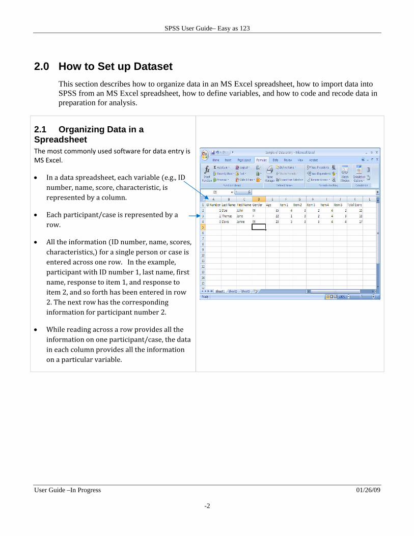
2.1 Organizing Data in a Spreadsheet The most commonly used software for data entry is MS Excel.

In a data spreadsheet, each variable e.g., ID

number, name, score, characteristic, is represented by a column.

Each participant/case is represented by a row.

All the information ID number, name, scores, characteristics, for a single person or case is entered across one row. In the example, participant with ID number 1, last name, first name, response to item 1, and response to item 2, and so forth has been entered in row 2. The next row has the corresponding information for participant number 2.

While reading across a row provides all the information on one participant/case, the data in each column provides all the information on a particular variable.



-3

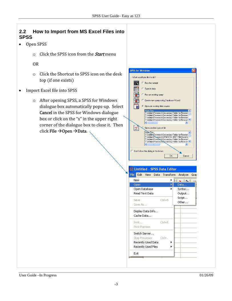
2.2 How to Import from MS Excel Files into SPSS Open SPSS

o Click the SPSS icon from the Start menu

OR

o Click the Shortcut to SPSS icon on the desk top if one exists

Import Excel file into SPSS

o After opening SPSS, a SPSS for Windows dialogue box automatically pops‐up. Select Cancel in the SPSS for Windows dialogue box or click on the “x” in the upper right corner of the dialogue box to close it. Then click File Open Data.



-4

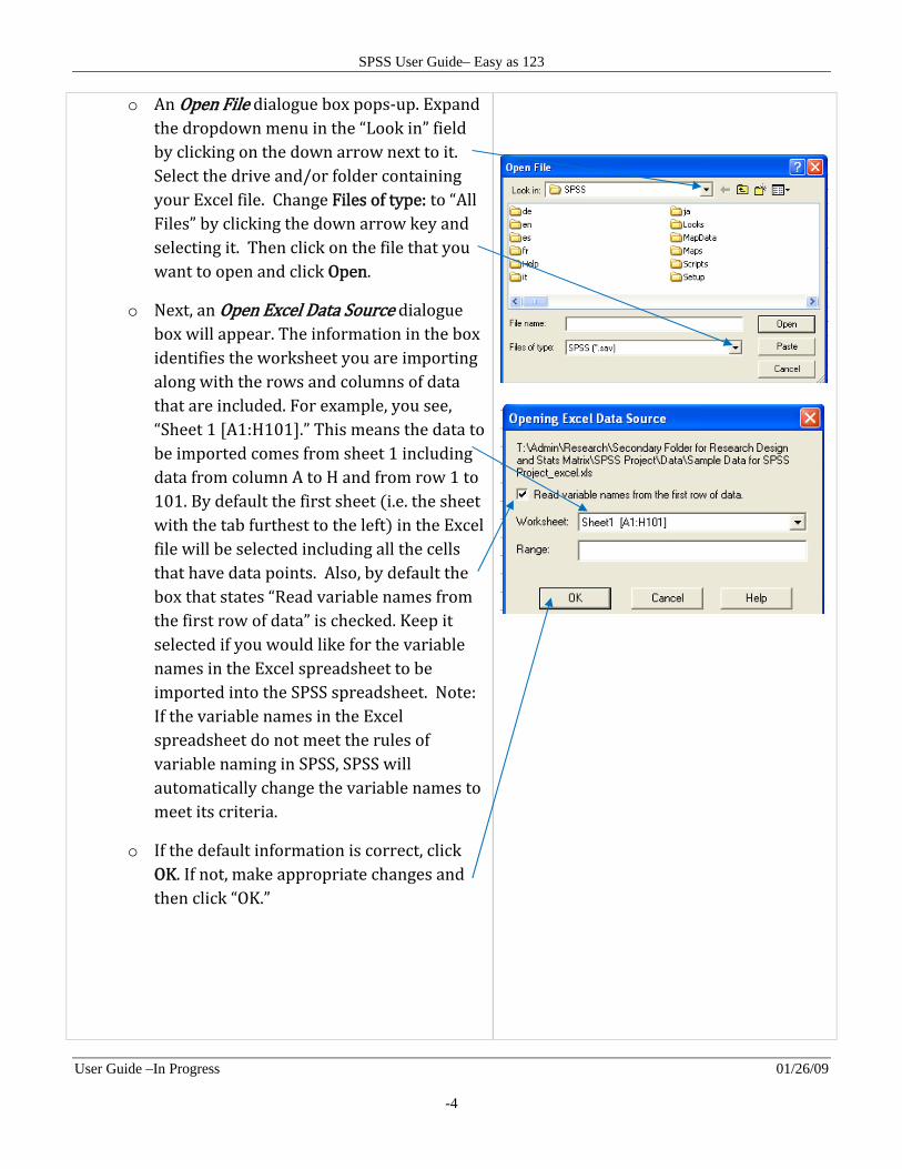
o An Open File dialogue box pops‐up. Expand the dropdown menu in the “Look in” field by clicking on the down arrow next to it. Select the drive and/or folder containing your Excel file. Change Files of type: to “All Files” by clicking the down arrow key and selecting it. Then click on the file that you want to open and click Open.

o Next, an Open Excel Data Source dialogue box will appear. The information in the box identifies the worksheet you are importing along with the rows and columns of data that are included. For example, you see, “Sheet 1 A1:H101 .” This means the data to be imported comes from sheet 1 including data from column A to H and from row 1 to 101. By default the first sheet i.e. the sheet with the tab furthest to the left in the Excel file will be selected including all the cells that have data points. Also, by default the box that states “Read variable names from the first row of data” is checked. Keep it selected if you would like for the variable names in the Excel spreadsheet to be imported into the SPSS spreadsheet. Note: If the variable names in the Excel spreadsheet do not meet the rules of variable naming in SPSS, SPSS will automatically change the variable names to meet its criteria.

o If the default information is correct, click OK. If not, make appropriate changes and then click “OK.”



-5

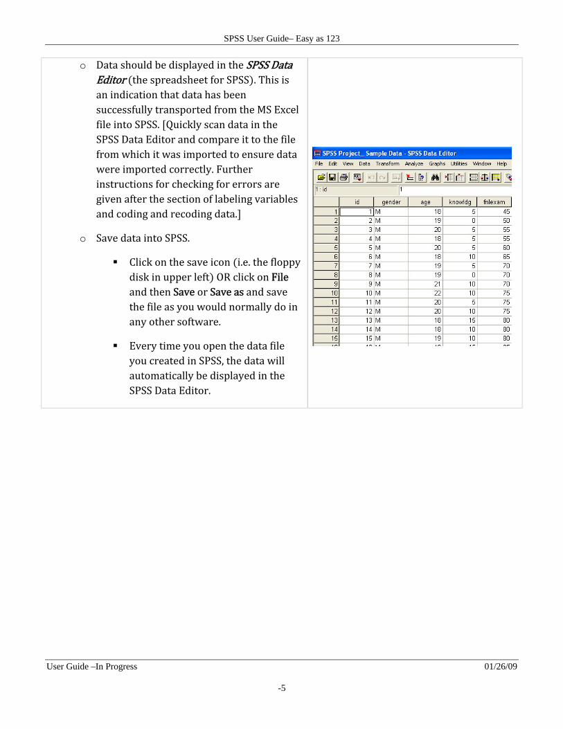
o Data should be displayed in the SPSS Data Editor the spreadsheet for SPSS . This is an indication that data has been successfully transported from the MS Excel file into SPSS. Quickly scan data in the SPSS Data Editor and compare it to the file from which it was imported to ensure data were imported correctly. Further instructions for checking for errors are given after the section of labeling variables and coding and recoding data.

o Save data into SPSS.

Click on the save icon i.e. the floppy disk in upper left OR click on File and then Save or Save as and save the file as you would normally do in any other software.

Every time you open the data file you created in SPSS, the data will automatically be displayed in the SPSS Data Editor.



-6

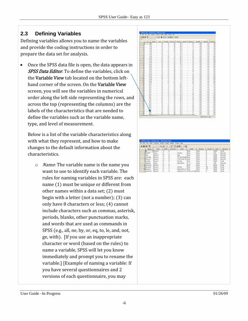
2.3 Defining Variables Defining variables allows you to name the variables and provide the coding instructions in order to prepare the data set for analysis.

Once the SPSS data file is open, the data appears in SPSS Data Editor. To define the variables, click on the Variable View tab located on the bottom left‐hand corner of the screen. On the Variable View screen, you will see the variables in numerical order along the left side representing the rows, and across the top representing the columns are the labels of the characteristics that are needed to define the variables such as the variable name, type, and level of measurement.

Below is a list of the variable characteristics along with what they represent, and how to make changes to the default information about the characteristics.

o Name: The variable name is the name you want to use to identify each variable. The rules for naming variables in SPSS are: each name 1 must be unique or different from other names within a data set; 2 must begin with a letter not a number ; 3 can only have 8 characters or less; 4 cannot include characters such as commas, asterisk, periods, blanks, other punctuation marks, and words that are used as commands in SPSS e.g., all, ne, by, or, eq, to, le, and, not, ge, with . If you use an inappropriate character or word based on the rules to name a variable, SPSS will let you know immediately and prompt you to rename the variable. Example of naming a variable: If you have several questionnaires and 2 versions of each questionnaire, you may



-7

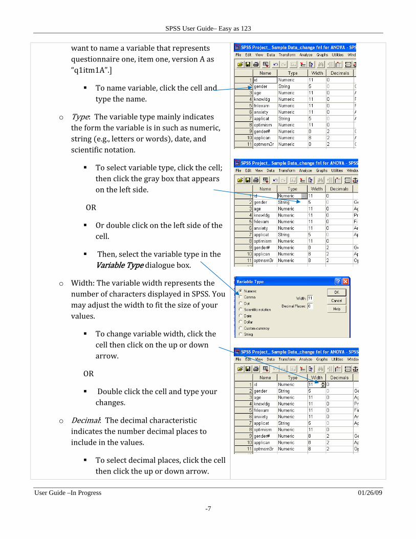
want to name a variable that represents questionnaire one, item one, version A as “q1itm1A”.

To name variable, click the cell and type the name.

o Type: The variable type mainly indicates the form the variable is in such as numeric, string e.g., letters or words , date, and scientific notation.

To select variable type, click the cell; then click the gray box that appears on the left side.

OR

Or double click on the left side of the cell.

Then, select the variable type in the Variable Type dialogue box.

o Width: The variable width represents the number of characters displayed in SPSS. You may adjust the width to fit the size of your values.

To change variable width, click the cell then click on the up or down arrow.

OR

Double click the cell and type your changes.

o Decimal: The decimal characteristic indicates the number decimal places to include in the values.

To select decimal places, click the cell then click the up or down arrow.



-8

OR

Double click the cell and type your changes.

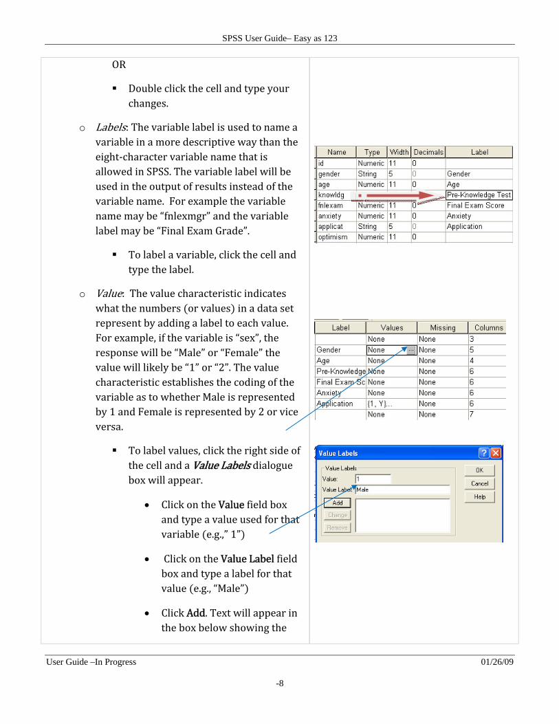
o Labels: The variable label is used to name a variable in a more descriptive way than the eight‐character variable name that is allowed in SPSS. The variable label will be used in the output of results instead of the variable name. For example the variable name may be “fnlexmgr” and the variable label may be “Final Exam Grade”.

To label a variable, click the cell and type the label.

o Value: The value characteristic indicates what the numbers or values in a data set represent by adding a label to each value. For example, if the variable is “sex”, the response will be “Male” or “Female” the value will likely be “1” or “2”. The value characteristic establishes the coding of the variable as to whether Male is represented by 1 and Female is represented by 2 or vice versa.

To label values, click the right side of the cell and a Value Labels dialogue box will appear.

Click on the Value field box and type a value used for that variable e.g.,” 1”

Click on the Value Label field box and type a label for that value e.g., “Male”

Click Add. Text will appear in the box below showing the



-9

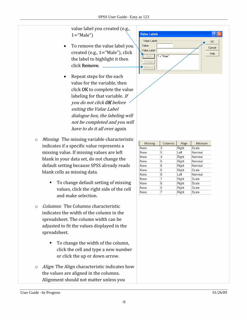
value label you created e.g., 1 ”Male”

To remove the value label you created e.g., 1 ”Male” , click the label to highlight it then click Remove.

Repeat steps for the each value for the variable, then click OK to complete the value labeling for that variable. If you do not click OK before exiting the Value Label dialogue box, the labeling will not be completed and you will have to do it all over again.

o Missing: The missing variable characteristic indicates if a specific value represents a missing value. If missing values are left blank in your data set, do not change the default setting because SPSS already reads blank cells as missing data.

To change default setting of missing values, click the right side of the cell and make selection.

o Columns: The Columns characteristic indicates the width of the column in the spreadsheet. The column width can be adjusted to fit the values displayed in the spreadsheet.

To change the width of the column, click the cell and type a new number or click the up or down arrow.

o Align: The Align characteristic indicates how the values are aligned in the columns. Alignment should not matter unless you



-10

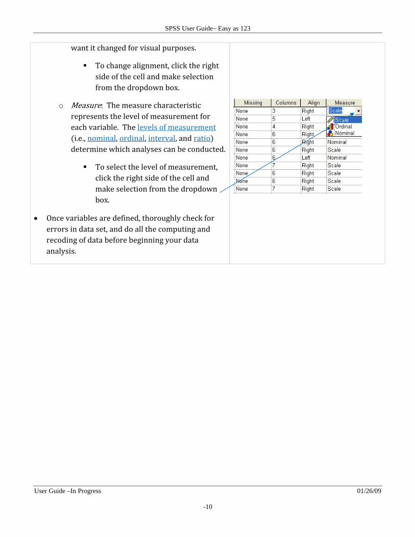
want it changed for visual purposes.

To change alignment, click the right side of the cell and make selection from the dropdown box.

o Measure: The measure characteristic represents the level of measurement for each variable. The levels of measurement i.e., nominal, ordinal, interval, and ratio determine which analyses can be conducted.

To select the level of measurement, click the right side of the cell and make selection from the dropdown box.

Once variables are defined, thoroughly check for errors in data set, and do all the computing and recoding of data before beginning your data analysis.



-11

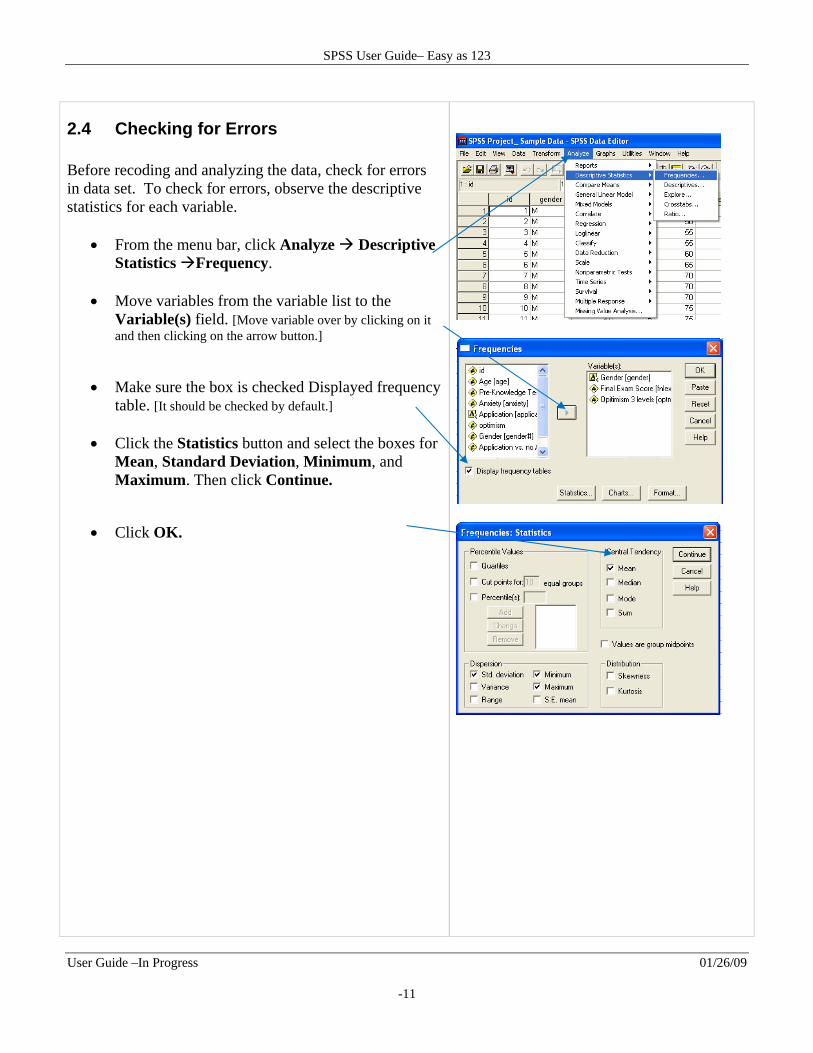
2.4 Checking for Errors Before recoding and analyzing the data, check for errors in data set. To check for errors, observe the descriptive statistics for each variable.

From the menu bar, click Analyze Descriptive Statistics Frequency.

Move variables from the variable list to the

Variable(s) field. [Move variable over by clicking on it and then clicking on the arrow button.]

Make sure the box is checked Displayed frequency table. [It should be checked by default.]

Click the Statistics button and select the boxes for

Mean, Standard Deviation, Minimum, and Maximum. Then click Continue.

Click OK.



-12

Output Generated

The first table, labeled Statistics, shows the descriptive statistics such as the overall sample size for the data set, and the Mean, Standard deviation, Minimum and Maximum scores for each variable.

The remaining tables in the output are Frequency Tables. Each table represents a variable. Each type of response/score is listed with the frequency/number of cases/participants with that response/score. For example if 50 out of 100 participants respond that they are female, the frequency for the response of female is 50 and the percentage is 50%.

For categorical variables such as gender, the frequency is the only meaningful statistic. Do not try to interpret the Mean and Standard Deviation. As can be seen in the first Table, SPSS did not provide any values for the statistics for the Gender variable. This is due to the variable not being coded yet with numerical values. [The coding and recoding process is explained in the next section.] The numerical values assigned to the categorical data are only used to differentiate the categories. The numbers have no meaning in regards to value or order. To check for errors for categorical variables:

Make sure only the categories that are supposed to be there are there. For, example if the variable is gender (Male or Female) and the frequency chart shows a third category, there is an error.

Make sure the frequencies for the categories look reasonable.

For continuous variables such as final exam score, all descriptive statistics can be interpreted.

To check for errors for continuous variables:

Observes the Minimum and Maximum scores and make sure the numbers do not fall outside the range of possible scores.

Observe the Mean and Standard deviation to make sure they look like what you expected.



-13

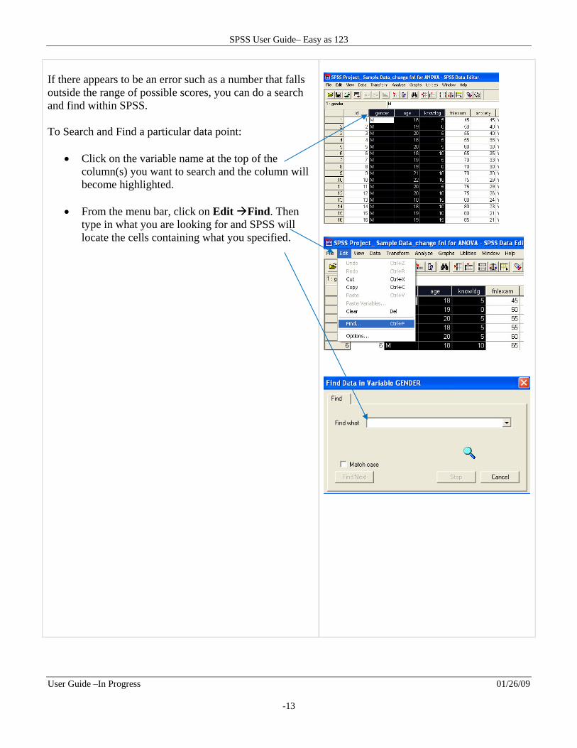
If there appears to be an error such as a number that falls outside the range of possible scores, you can do a search and find within SPSS. To Search and Find a particular data point:

Click on the variable name at the top of the column(s) you want to search and the column will become highlighted.

From the menu bar, click on Edit Find. Then type in what you are looking for and SPSS will locate the cells containing what you specified.



-14

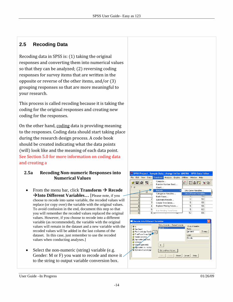
2.5 Recoding Data Recoding data in SPSS is: 1 taking the original responses and converting them into numerical values so that they can be analyzed; 2 reversing coding responses for survey items that are written in the opposite or reverse of the other items, and/or 3 grouping responses so that are more meaningful to your research.

This process is called recoding because it is taking the coding for the original responses and creating new coding for the responses.

On the other hand, coding data is providing meaning to the responses. Coding data should start taking place during the research design process. A code book should be created indicating what the data points will look like and the meaning of each data point. See Section 5.0 for more information on coding data and creating a

2.5a Recoding Nonnumeric Responses into Numerical Values

From the menu bar, click Transform Recode Into Different Variables… [Please note, if you choose to recode into same variable, the recoded values will replace (or copy over) the variable with the original values. To avoid confusion in the end, document this step so that you will remember the recoded values replaced the original values. However, if you choose to recode into a different variable (as recommended), the variable with the original values will remain in the dataset and a new variable with the recoded values will be added in the last column of the dataset. In this case, just remember to use the recoded values when conducting analyses.]

Select the non-numeric (string) variable (e.g.

Gender: M or F) you want to recode and move it to the string to output variable conversion box.



-15

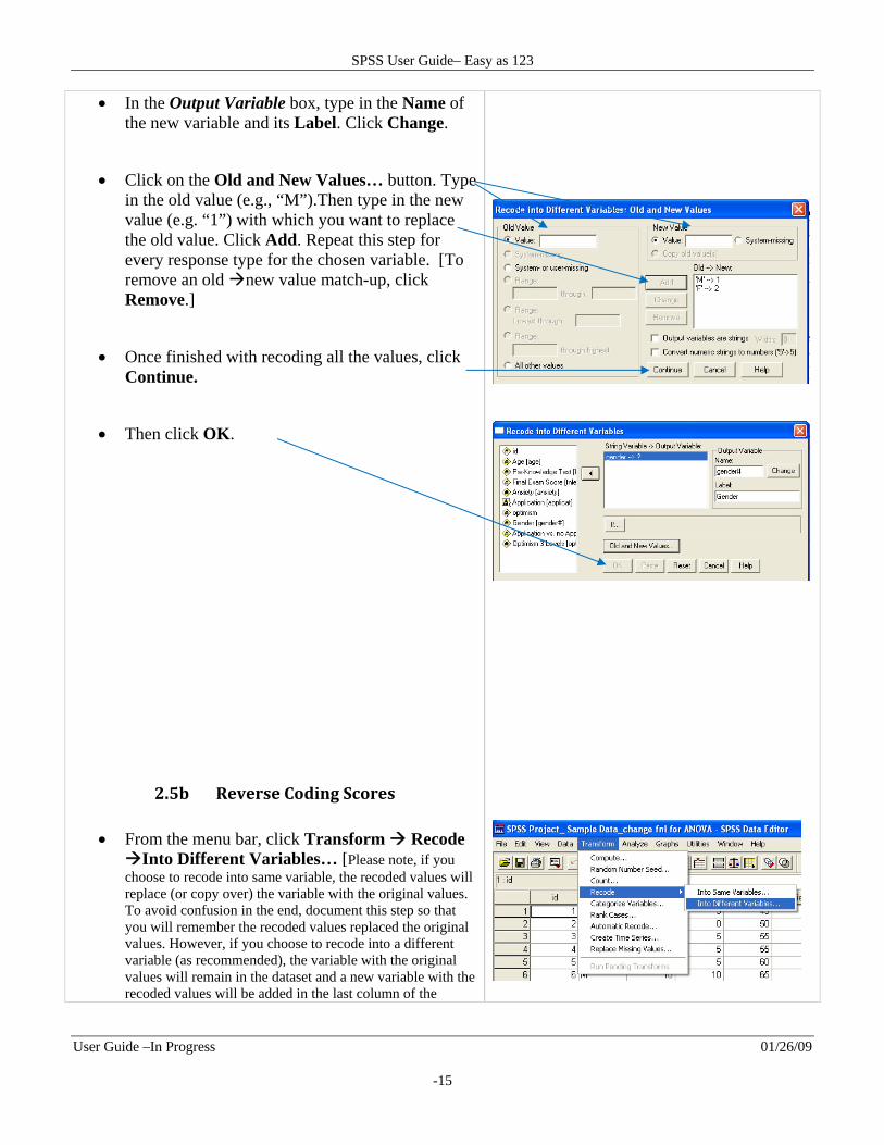
In the Output Variable box, type in the Name of the new variable and its Label. Click Change.

Click on the Old and New Values… button. Type in the old value (e.g., “M”).Then type in the new value (e.g. “1”) with which you want to replace the old value. Click Add. Repeat this step for every response type for the chosen variable. [To remove an old new value match-up, click Remove.]

Once finished with recoding all the values, click Continue.

Then click OK.

2.5b Reverse Coding Scores

From the menu bar, click Transform Recode Into Different Variables… [Please note, if you choose to recode into same variable, the recoded values will replace (or copy over) the variable with the original values. To avoid confusion in the end, document this step so that you will remember the recoded values replaced the original values. However, if you choose to recode into a different variable (as recommended), the variable with the original values will remain in the dataset and a new variable with the recoded values will be added in the last column of the



-16

dataset. In this case, just remember to use the recoded values when conducting analyses.]

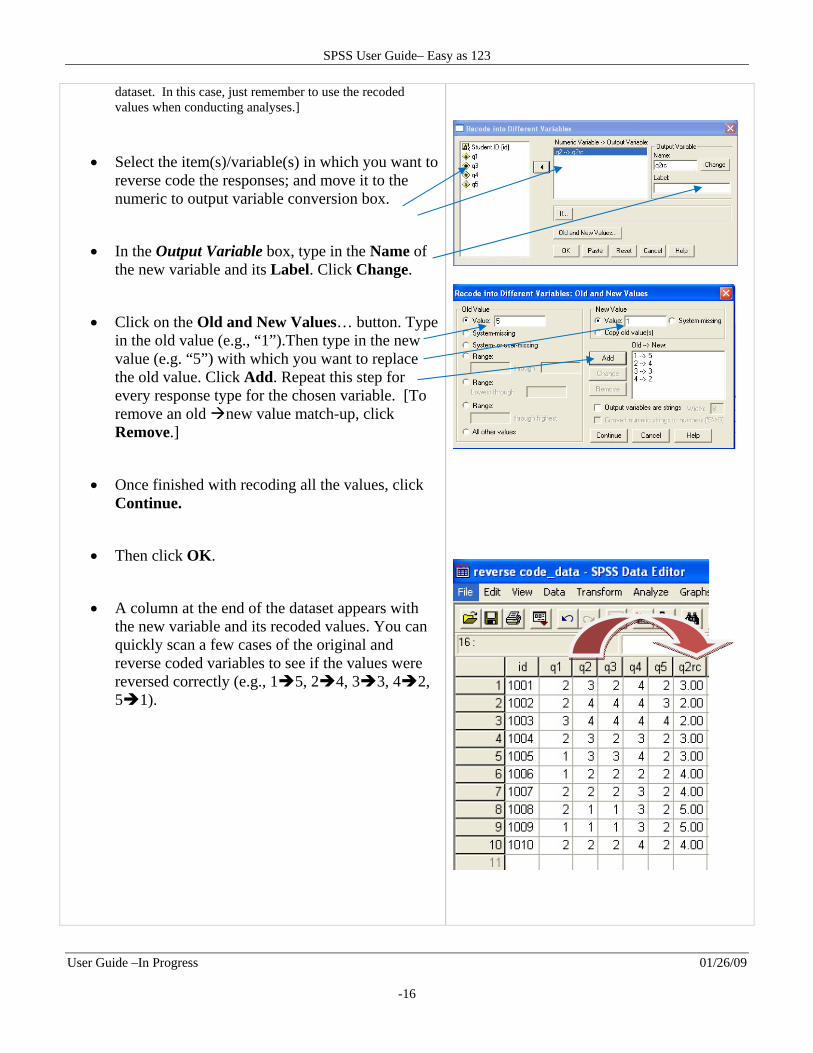
Select the item(s)/variable(s) in which you want to reverse code the responses; and move it to the numeric to output variable conversion box.


Click on the Old and New Values… button. Type in the old value (e.g., “1”).Then type in the new value (e.g. “5”) with which you want to replace the old value. Click Add. Repeat this step for every response type for the chosen variable. [To remove an old new value match-up, click Remove.]


Then click OK.

A column at the end of the dataset appears with the new variable and its recoded values. You can quickly scan a few cases of the original and reverse coded variables to see if the values were reversed correctly (e.g., 15, 24, 33, 42, 51).



-17

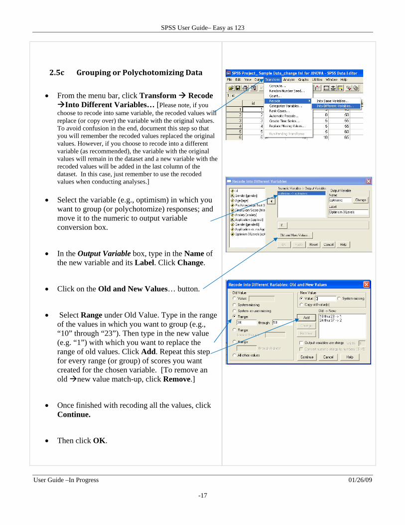
2.5c Grouping or Polychotomizing Data

From the menu bar, click Transform Recode Into Different Variables… [Please note, if you choose to recode into same variable, the recoded values will replace (or copy over) the variable with the original values. To avoid confusion in the end, document this step so that you will remember the recoded values replaced the original values. However, if you choose to recode into a different variable (as recommended), the variable with the original values will remain in the dataset and a new variable with the recoded values will be added in the last column of the dataset. In this case, just remember to use the recoded values when conducting analyses.]

Select the variable (e.g., optimism) in which you want to group (or polychotomize) responses; and move it to the numeric to output variable conversion box.


Click on the Old and New Values… button.

Select Range under Old Value. Type in the range of the values in which you want to group (e.g., “10” through “23”). Then type in the new value (e.g. “1”) with which you want to replace the range of old values. Click Add. Repeat this step for every range (or group) of scores you want created for the chosen variable. [To remove an old new value match-up, click Remove.]


Then click OK.



-18

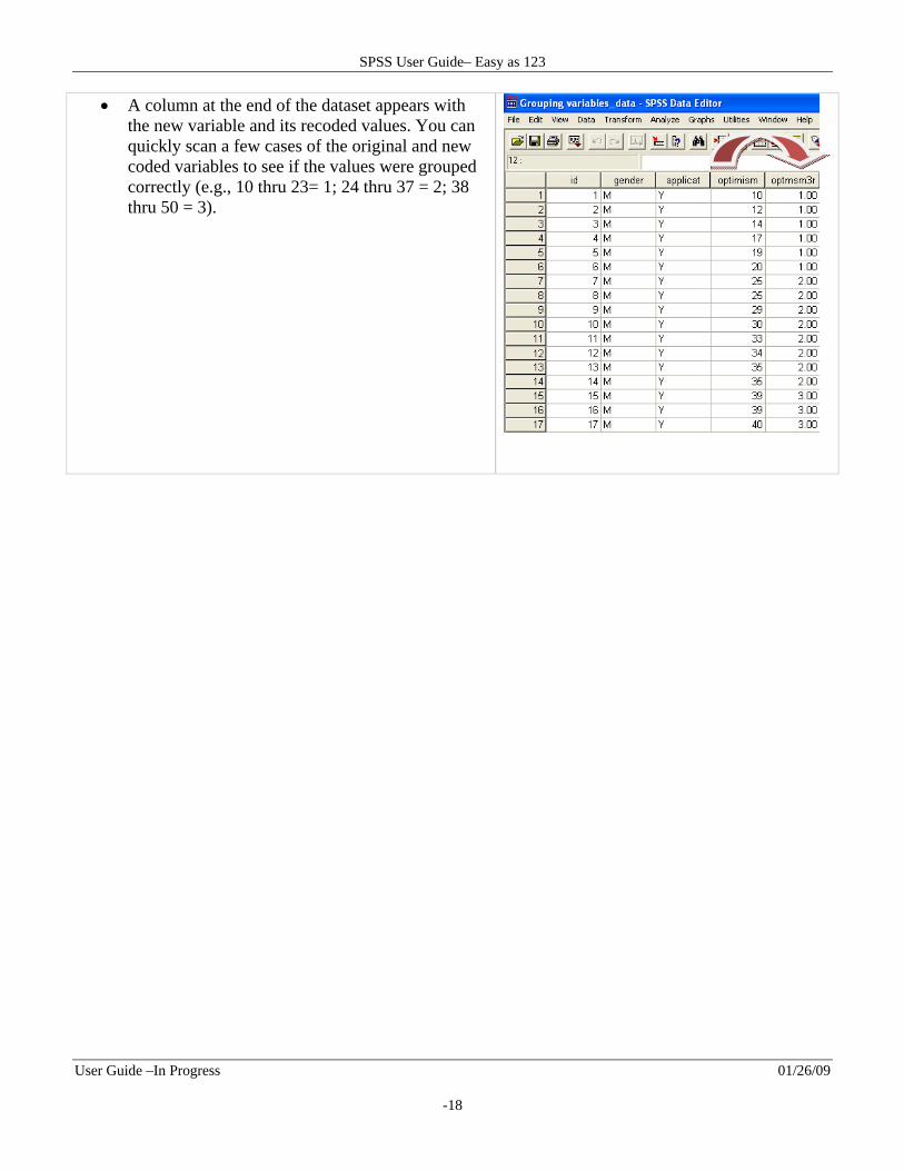
A column at the end of the dataset appears with the new variable and its recoded values. You can quickly scan a few cases of the original and new coded variables to see if the values were grouped correctly (e.g., 10 thru 23= 1; 24 thru 37 = 2; 38 thru 50 = 3).



-19

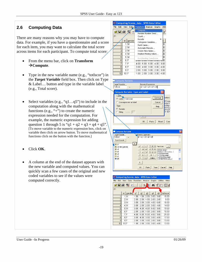
2.6 Computing Data There are many reasons why you may have to compute data. For example, if you have a questionnaire and a score for each item, you may want to calculate the total score across items for each participant. To compute total score:

From the menu bar, click on Transform Compute.

Type in the new variable name (e.g., “totlscor”) in the Target Variable field box. Then click on Type & Label… button and type in the variable label (e.g., Total score).

Select variables (e.g., “q1…q5”) to include in the computation along with the mathematical functions (e.g., “+”) to create the numeric expression needed for the computation. For example, the numeric expression for adding question 1 through 5 is “q1 + q2 + q3 + q4 + q5”. [To move variable to the numeric expression box, click on variable then click on arrow button. To move mathematical functions click on the button with the function.]

Click OK.

A column at the end of the dataset appears with the new variable and computed values. You can quickly scan a few cases of the original and new coded variables to see if the values were computed correctly.



-20

3.0 How to Analyze Data in SPSS

This section describes how to run different types of statistical analyses in SPSS (version 11.5) and interpret the output of results. Only the most common statistical methods used in the Scholarship of Teaching and Learning (SoTL) research are discussed in this section. [More statistical techniques will be added at a later date]

List of statistical methods that will be added:

Chi-square

Two-way ANOVA

ANCOVA

Multiple Regression



-21

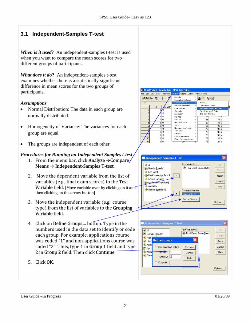
3.1 Independent-Samples T-test When is it used? An independent-samples t-test is used when you want to compare the mean scores for two different groups of participants. What does it do? An independent-samples t-test examines whether there is a statistically significant difference in mean scores for the two groups of participants. Assumptions Normal Distribution: The data in each group are

normally distributed.

Homogeneity of Variance: The variances for each group are equal.

The groups are independent of each other.

Procedures for Running an Independent Samples t-test 1. From the menu bar, click Analyze Compare

Means Independent‐Samples T‐test.

2. Move the dependent variable from the list of variables e.g., final exam scores to the Test Variable field. Move variable over by clicking on it and then clicking on the arrow button

3. Move the independent variable e.g., course type from the list of variables to the Grouping Variable field.

4. Click on Define Groups… button. Type in the numbers used in the data set to identify or code each group. For example, applications course was coded “1” and non‐applications course was coded “2”. Thus, type 1 in Group 1 field and type 2 in Group 2 field. Then click Continue.

5. Click OK.



-22

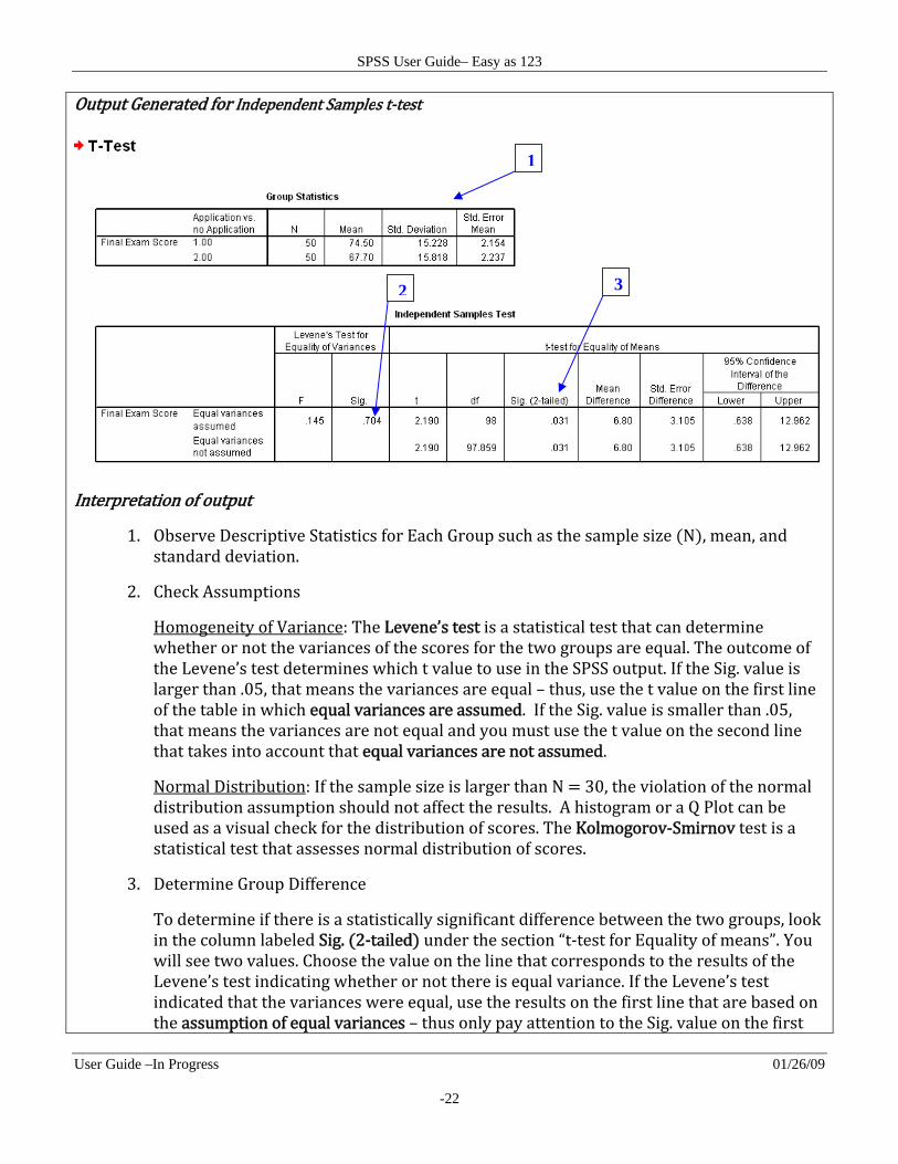
Output Generated for Independent Samples t‐test

Interpretation of output

1. Observe Descriptive Statistics for Each Group such as the sample size N , mean, and standard deviation.

2. Check Assumptions

Homogeneity of Variance: The Levene’s test is a statistical test that can determine whether or not the variances of the scores for the two groups are equal. The outcome of the Levene’s test determines which t value to use in the SPSS output. If the Sig. value is larger than .05, that means the variances are equal – thus, use the t value on the first line of the table in which equal variances are assumed. If the Sig. value is smaller than .05, that means the variances are not equal and you must use the t value on the second line that takes into account that equal variances are not assumed.

Normal Distribution: If the sample size is larger than N 30, the violation of the normal distribution assumption should not affect the results. A histogram or a Q Plot can be used as a visual check for the distribution of scores. The Kolmogorov‐Smirnov test is a statistical test that assesses normal distribution of scores.

3. Determine Group Difference

To determine if there is a statistically significant difference between the two groups, look in the column labeled Sig. 2‐tailed under the section “t‐test for Equality of means”. You will see two values. Choose the value on the line that corresponds to the results of the Levene’s test indicating whether or not there is equal variance. If the Levene’s test indicated that the variances were equal, use the results on the first line that are based on the assumption of equal variances – thus only pay attention to the Sig. value on the first

1

2 3



-23

line. If the equal variances assumption is violated, use the information on the second line.

If the Sig. 2‐tailed value of the t‐test is equal to or less than .05, there is a significant difference between the two groups. On the other hand, if Sig. 2‐tailed value of the t‐test is greater than .05, there is no statistically significant difference between the groups.

4. Determine the Effect Size

Even though we know whether or not there is a statistically significant difference between the scores, SPSS does not calculate the degree or magnitude of the difference i.e., the effect size . Thus, you have to calculate it on your own. The statistic used to determine the effect size is Eta squared. The formula for eta squared for an independent‐samples t‐test is t2 / t2 N1 N2 ‐2 .

For this example eta squared is 2.192 / 2.192 50 50 – 2 .0466

Guide for eta squared values: .01 small effect, .06 moderate effect, .14 large effect Cohen, 1988

Interpretation of eta squared: Multiply eta squared value e.g. .0466 by 100. That new value 4.66 becomes the percent of variance accounted for in the dependent variable e.g., exam score by the independent variable e.g. type of course .

Writing‐up Results

An independent‐samples t‐test was conducted to compare final exam scores for students in an applications course and students in a non‐applications course. There was a significant difference in final exam scores for students in an applications course M 74.50, SD 15.23 , and students in a non‐applications course M 67.70, SD 15.82 ; t 98 2.19, p .03. The magnitude of the difference was large eta squared .047 .



-24

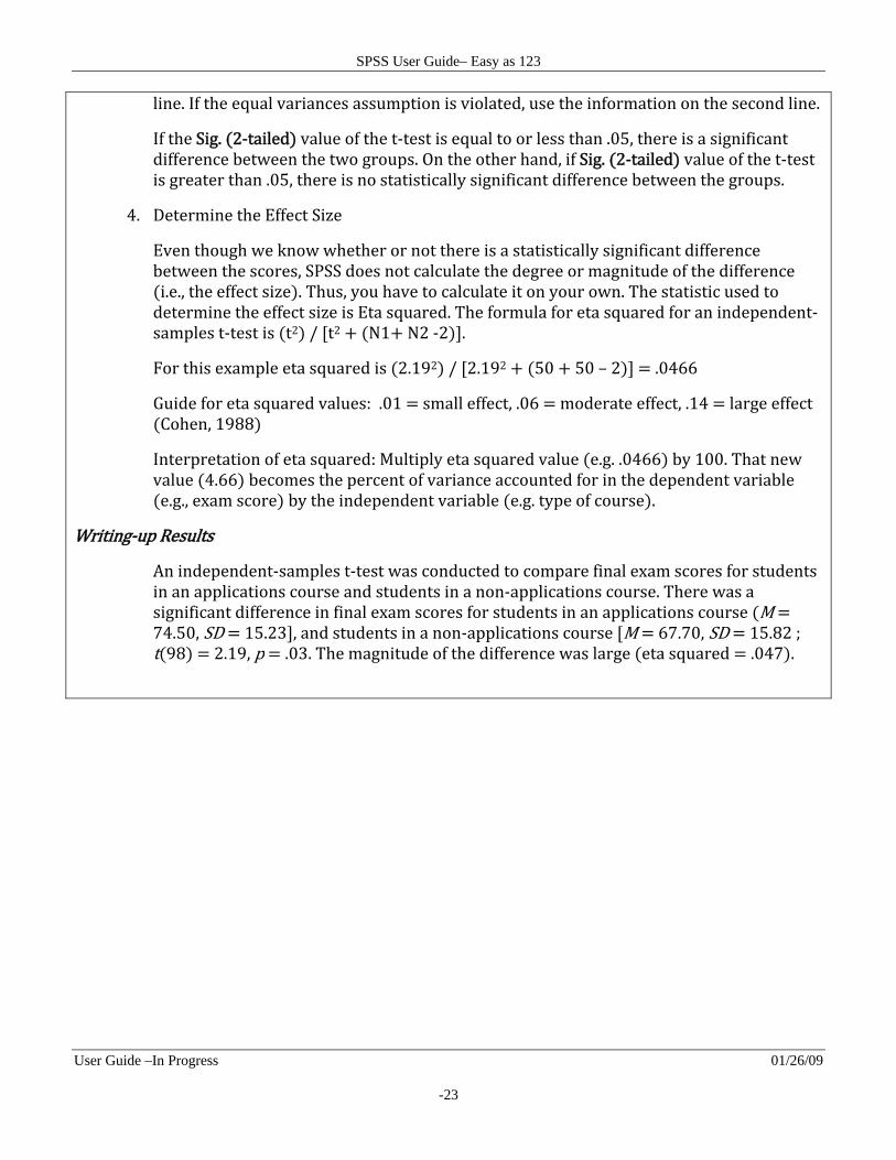
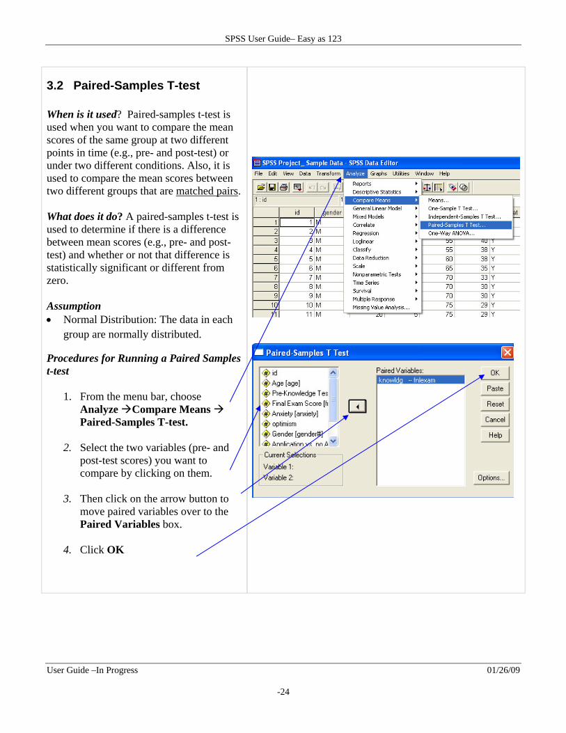
3.2 Paired-Samples T-test When is it used? Paired-samples t-test is used when you want to compare the mean scores of the same group at two different points in time (e.g., pre- and post-test) or under two different conditions. Also, it is used to compare the mean scores between two different groups that are matched pairs. What does it do? A paired-samples t-test is used to determine if there is a difference between mean scores (e.g., pre- and post-test) and whether or not that difference is statistically significant or different from zero. Assumption Normal Distribution: The data in each

group are normally distributed.

Procedures for Running a Paired Samples t-test

1. From the menu bar, choose Analyze Compare Means Paired-Samples T-test.

2. Select the two variables (pre- and

post-test scores) you want to compare by clicking on them.

3. Then click on the arrow button to

move paired variables over to the Paired Variables box.

4. Click OK



-25

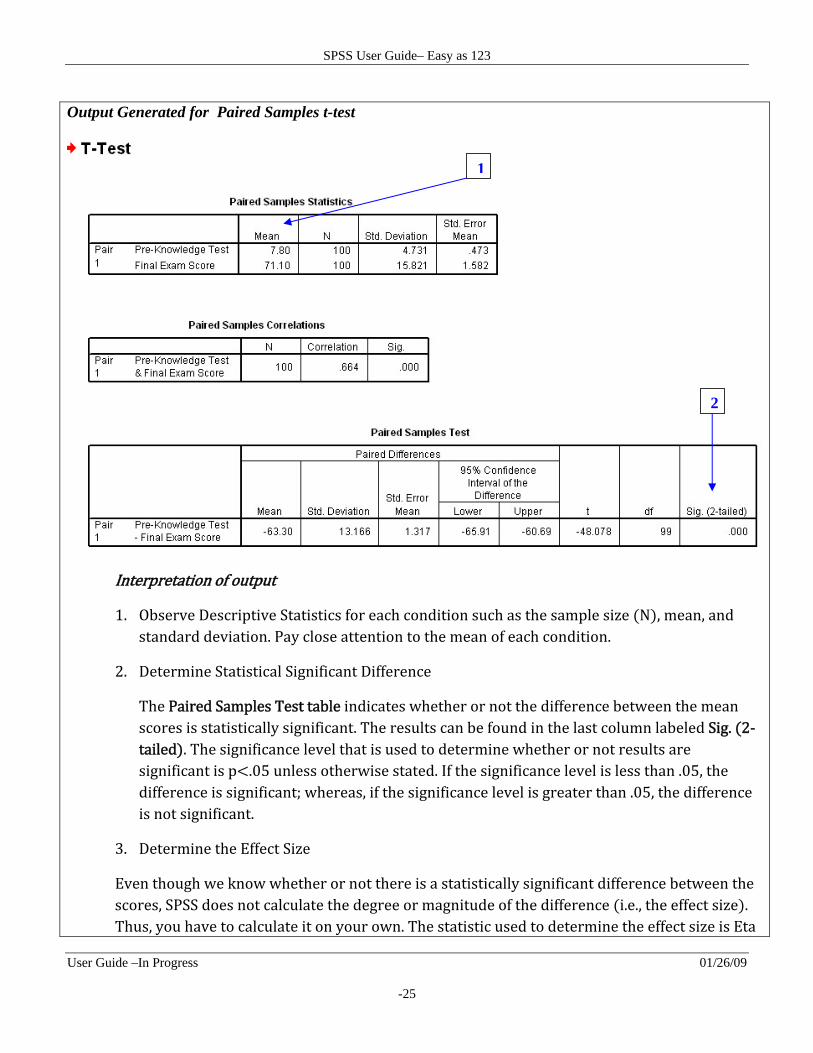
Output Generated for Paired Samples t-test


1. Observe Descriptive Statistics for each condition such as the sample size N , mean, and standard deviation. Pay close attention to the mean of each condition.

2. Determine Statistical Significant Difference

The Paired Samples Test table indicates whether or not the difference between the mean scores is statistically significant. The results can be found in the last column labeled Sig. 2‐tailed . The significance level that is used to determine whether or not results are significant is p .05 unless otherwise stated. If the significance level is less than .05, the difference is significant; whereas, if the significance level is greater than .05, the difference is not significant.


Even though we know whether or not there is a statistically significant difference between the scores, SPSS does not calculate the degree or magnitude of the difference i.e., the effect size .Thus, you have to calculate it on your own. The statistic used to determine the effect size is Eta

1

2



-26

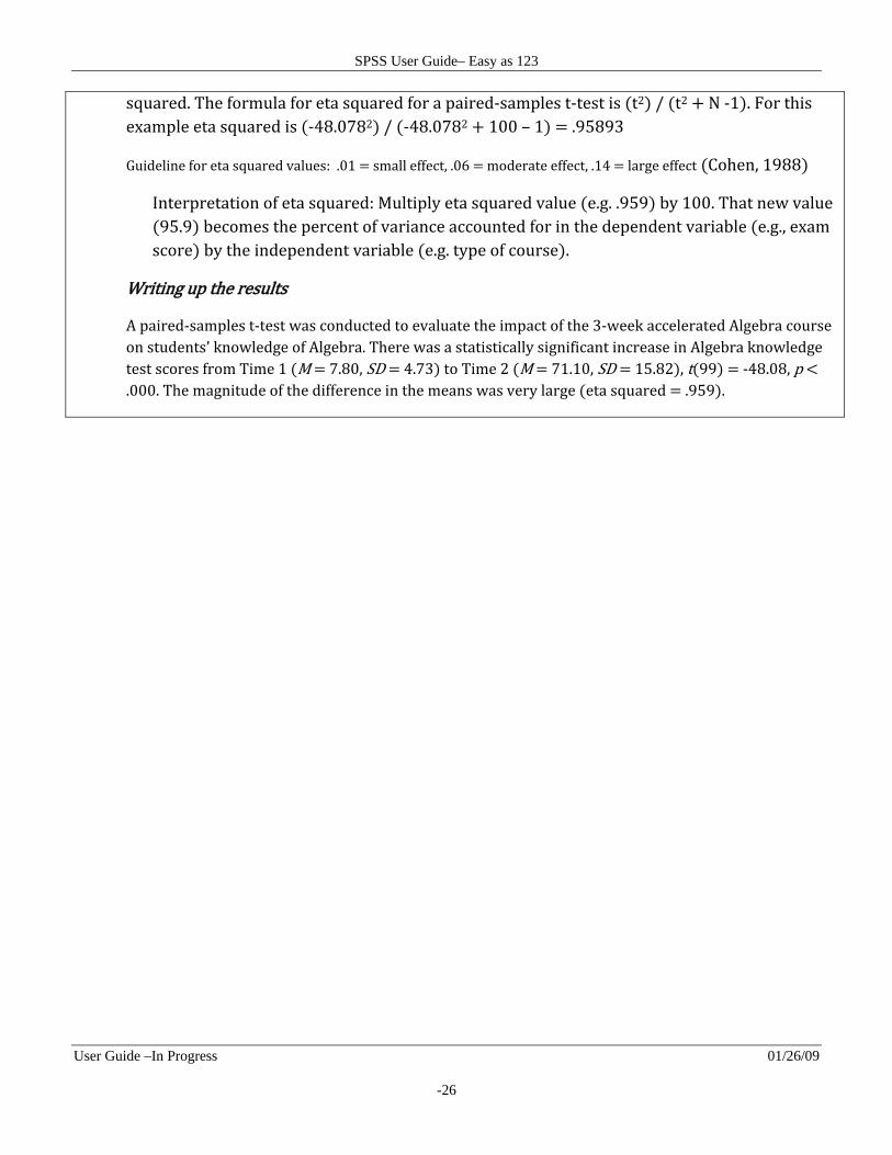
squared. The formula for eta squared for a paired‐samples t‐test is t2 / t2 N ‐1 . For this example eta squared is ‐48.0782 / ‐48.0782 100 – 1 .95893

Guideline for eta squared values: .01 small effect, .06 moderate effect, .14 large effect Cohen, 1988


Writing up the results

A paired‐samples t‐test was conducted to evaluate the impact of the 3‐week accelerated Algebra course on students’ knowledge of Algebra. There was a statistically significant increase in Algebra knowledge test scores from Time 1 M 7.80, SD 4.73 to Time 2 M 71.10, SD 15.82 , t 99 ‐48.08, p .000. The magnitude of the difference in the means was very large eta squared .959 .



-27

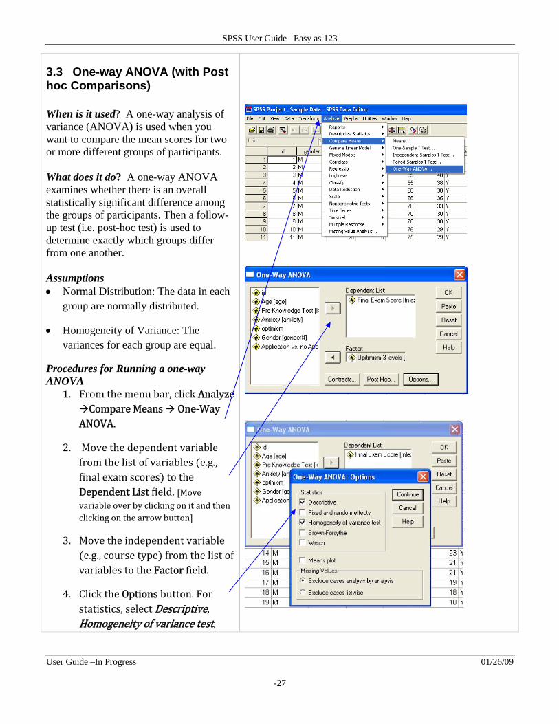
3.3 One-way ANOVA (with Post hoc Comparisons) When is it used? A one-way analysis of variance (ANOVA) is used when you want to compare the mean scores for two or more different groups of participants. What does it do? A one-way ANOVA examines whether there is an overall statistically significant difference among the groups of participants. Then a follow-up test (i.e. post-hoc test) is used to determine exactly which groups differ from one another. Assumptions Normal Distribution: The data in each



Procedures for Running a one-way ANOVA

1. From the menu bar, click Analyze Compare Means One‐Way ANOVA.

2. Move the dependent variable from the list of variables e.g., final exam scores to the Dependent List field. Move variable over by clicking on it and then clicking on the arrow button

3. Move the independent variable e.g., course type from the list of variables to the Factor field.

4. Click the Options button. For statistics, select Descriptive, Homogeneity of variance test,



-28

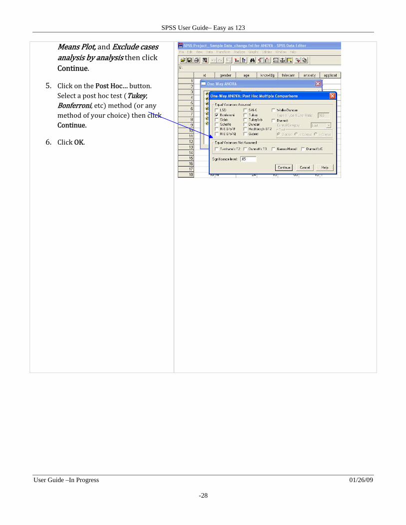
Means Plot, and Exclude cases analysis by analysis then click Continue.

5. Click on the Post Hoc… button. Select a post hoc test Tukey, Bonferroni, etc method or any method of your choice then click Continue.

6. Click OK.



-29

Output Generated for One-way ANOVA with Post-hoc Comparisons

1

2

3

4



-30


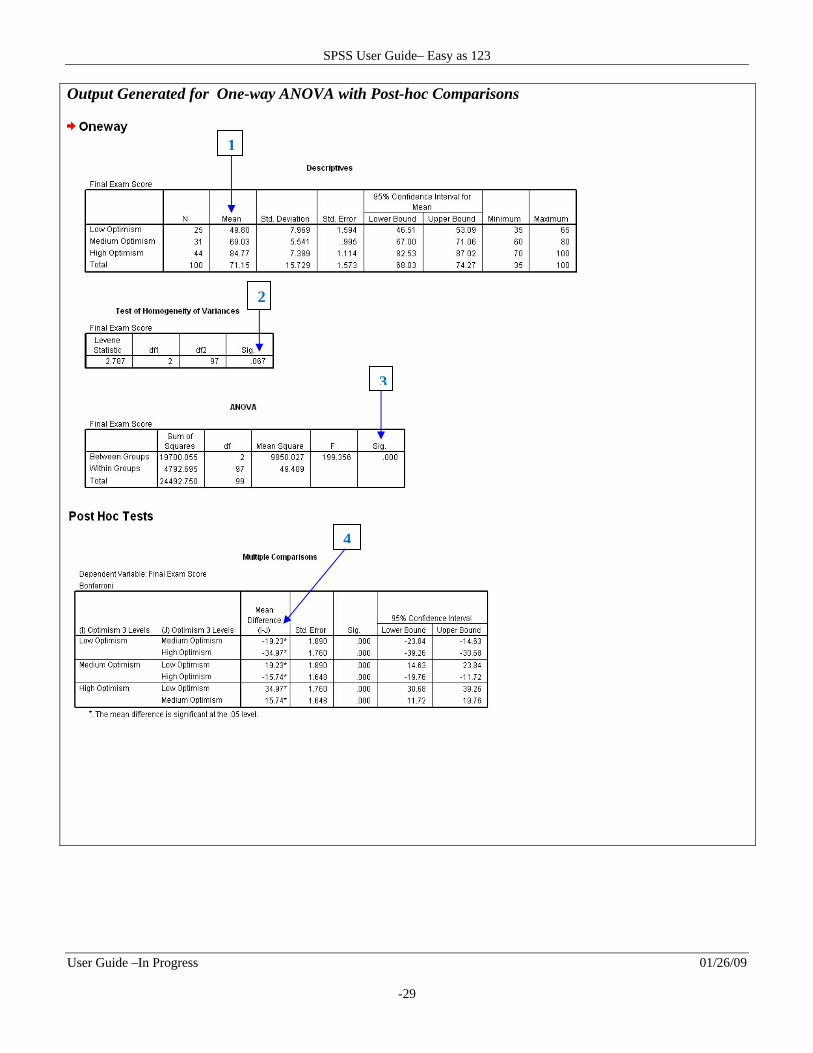
1. Observe Descriptive Statistics for each group/condition such as the sample size N , mean, and standard deviation.

2. Check the second table labeled Test of Homogeneity of Variance to determine if the groups have equal variance. If the significance level is greater than .05 the variances are equal; whereas, if the significance level is less than .05, the variances are not equal which means there is a violation of the assumption of homogeneity of variance.

3. Determine Overall Difference

The third table labeled ANOVA indicates whether or not there is a statistically significant overall difference in mean scores across the groups of participants. If the value in the last column labeled Sig is less than .05, there is a statistically significant difference; whereas, if the value is greater than .05, the difference is not statistically significant.

4. Determine Which Groups Are Different From Each Other

If the significance test for an ANOVA shows that there is an overall difference, the next step is to determine where the differences lie i.e. between which pair of groups . A post‐hoc test is a statistical test used to make comparisons between each pair of groups. The results of the post hoc tests can be found in the Multiple Comparison table. In this table, the mean difference is indicated for each pair of groups. If there is an asterisk next to the value of the group Mean Difference, it is statistically significant. In this example, the Bonferonni correction was used for the post‐hoc test. This method controls for Type I error.


Even though we know whether or not there is a statistically significant difference between the mean scores, SPSS does not calculate the degree or magnitude of the difference i.e., the effect size . Thus, you have to calculate it on your own. The statistic



-31

used to determine the effect size is Eta squared. The formula for eta squared for a one‐way ANOVA is Sum of squares between groups / Total sum of squares . From the results in the output, eta squared is 19700.005 / 24492.750 0.80432.




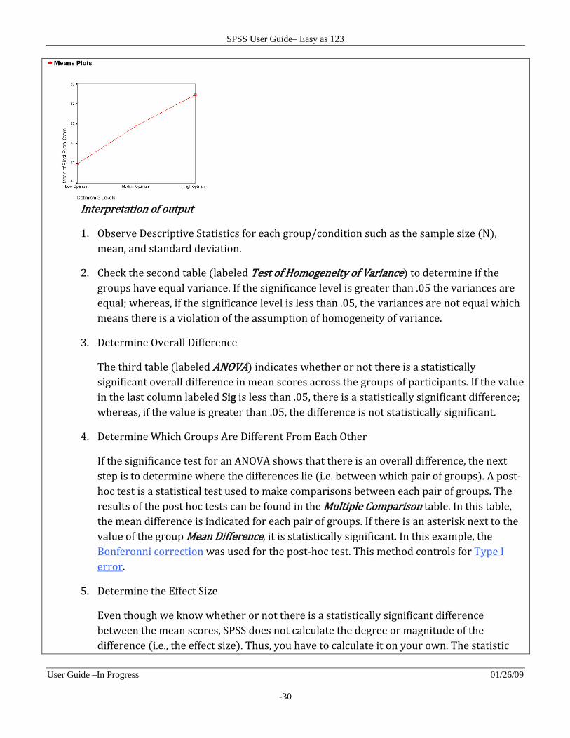
A one‐way ANOVA was conducted to evaluate the impact of optimism on test performance. Optimism was measured by the General Optimism test GOT and scores on a knowledge based test was used to represent test performance. Participants were divided into three groups based on their level of optimism. Group 1, 2 and 3, represented Low, Medium and High levels of optimism, respectively. Results showed that there was a statistically significant difference in knowledge test scores for the three levels of optimism groups F 2, 97 199.36, p .001 . The effect size was very large eta squared .80 . Post‐hoc comparisons using Bonferroni correction showed that the mean score for each group was statistically significant from each other. Group 1 M 49.80, SD 7.99 was statistically different from Group 2 M 69.03, SD 5.54 . Group 1 was statistically different from Group 3 M 84.77, SD 7.39 . Also, Group 2 was statistically significant different from Group 3. As indicated by the knowledge test mean scores and depicted in the graph, higher levels of optimism results in better test performance.



-32

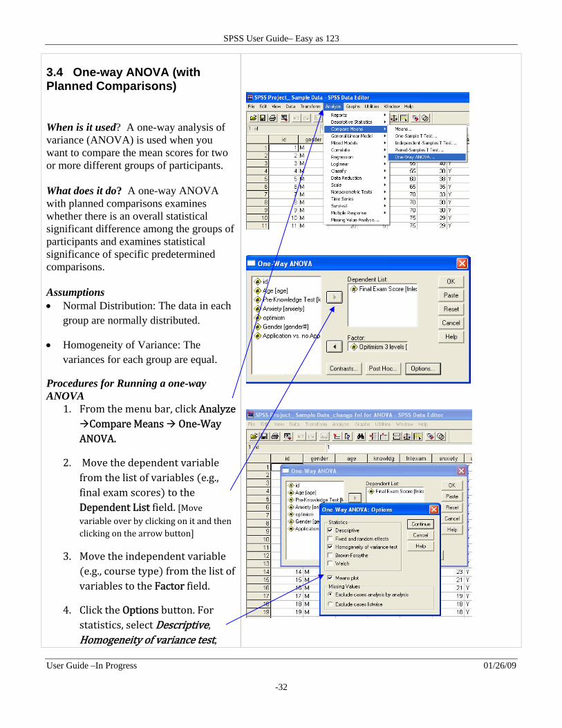
3.4 One-way ANOVA (with Planned Comparisons) When is it used? A one-way analysis of variance (ANOVA) is used when you want to compare the mean scores for two or more different groups of participants. What does it do? A one-way ANOVA with planned comparisons examines whether there is an overall statistical significant difference among the groups of participants and examines statistical significance of specific predetermined comparisons. Assumptions Normal Distribution: The data in each



Procedures for Running a one-way ANOVA

1. From the menu bar, click Analyze Compare Means One‐Way ANOVA.

2. Move the dependent variable from the list of variables e.g., final exam scores to the Dependent List field. Move variable over by clicking on it and then clicking on the arrow button

3. Move the independent variable e.g., course type from the list of variables to the Factor field.

4. Click the Options button. For statistics, select Descriptive, Homogeneity of variance test,



-33

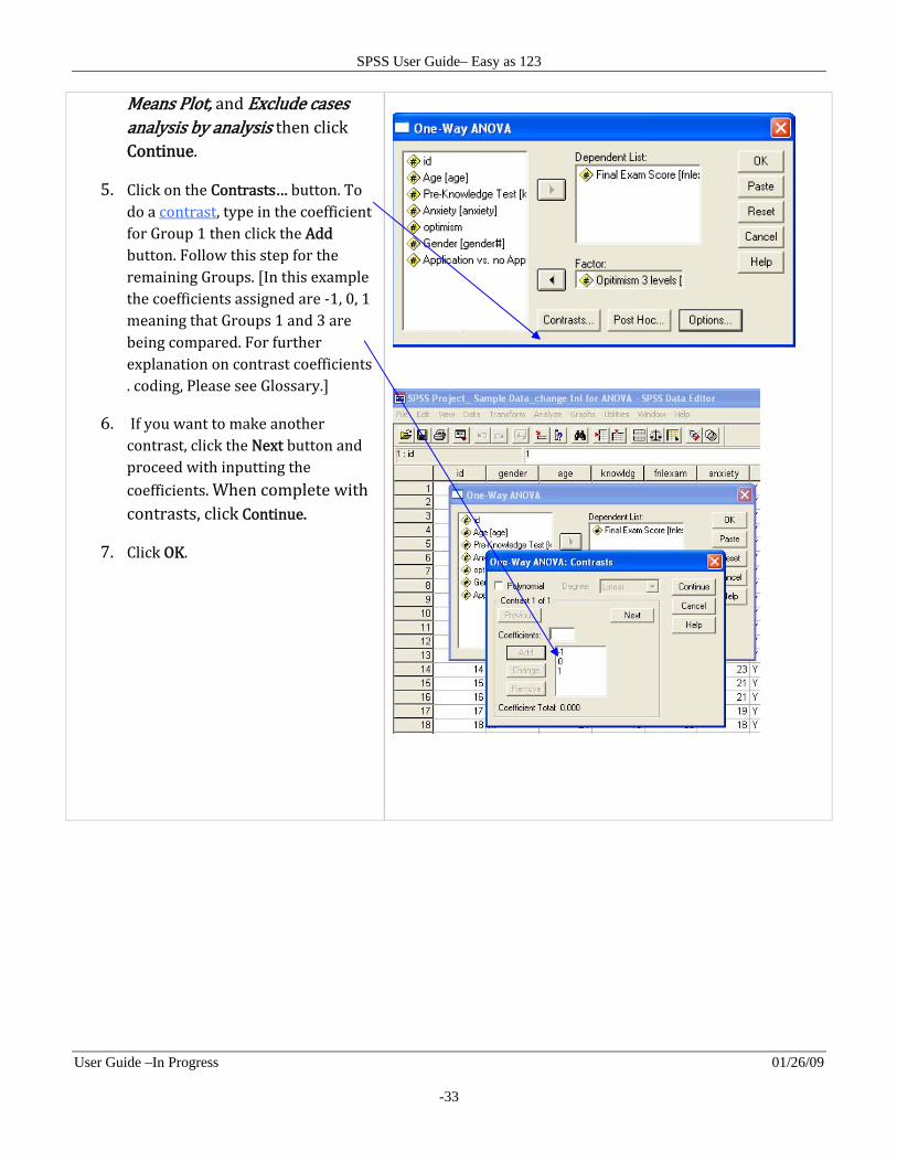
Means Plot, and Exclude cases analysis by analysis then click Continue.

5. Click on the Contrasts… button. To do a contrast, type in the coefficient for Group 1 then click the Add button. Follow this step for the remaining Groups. In this example the coefficients assigned are ‐1, 0, 1 meaning that Groups 1 and 3 are being compared. For further explanation on contrast coefficients . coding, Please see Glossary.

6. If you want to make another contrast, click the Next button and proceed with inputting the coefficients. When complete with contrasts, click Continue.

7. Click OK.



-34

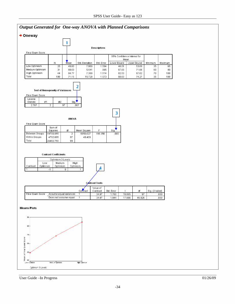
Output Generated for One-way ANOVA with Planned Comparisons

1

2

3

4



-35


1. Observe Descriptive Statistics for each group/condition such as the sample size N , mean, and standard deviation.

2. Check the second table labeled Test of Homogeneity of Variance to determine if the groups have equal variance. If the significance level is greater than .05 the variances are equal; whereas, if the significance level is less than .05, the variances are not equal which means there is a violation of the assumption of homogeneity of variance.

3. Determine Overall Difference

The third table labeled ANOVA indicates whether or not there is a statistically significant overall difference in mean scores across the groups of participants. If the value in the last column labeled Sig is less than .05, there is a statistically significant difference; whereas, if the value is greater than .05, the difference is not statistically significant.

4. Determine Difference for Pre‐specified/Planned Group Comparisons

For planned comparisons, check the Contrasts Coefficient table to make sure the coefficients match up your intended planned comparison s . The next table, labeled Contrast Tests, includes a statistical test for the pre‐specified comparison s . Due to the comparisons being broken down into pairs, a t‐statistic is given in analysis. To obtain an F value that represents the statistic for an ANOVA, the t value must be squared.


Even though we know whether or not there is a statistically significant difference between the mean scores, SPSS does not calculate the degree or magnitude of the difference i.e., the effect size . Thus, you have to calculate it on your own. The statistic used to determine the effect size is Eta squared. The formula for eta squared for a one‐way ANOVA is Sum of squares between groups / Total sum of squares . From the results in the output, eta squared is 19700.005 / 24492.750 0.80432.





-36


A one‐way ANOVA was conducted to evaluate the impact of optimism on test performance. Optimism was measured by the General Optimism test GOT and scores on a knowledge based test was used to represent test performance. Participants were divided into three groups based on their level of optimism. Group 1, 2 and 3, represented Low, Medium and High levels of optimism, respectively. Results showed that there was a statistically significant difference in knowledge test scores for the three levels of optimism groups F 2, 97 199.36, p .001 . The effect size was very large eta squared .80 . A planned comparison contrasting Group 1 and 3 was conducted. The difference between the mean scores of Group 1 M 49.80, SD 7.99 and Group 3 M 84.77, SD 7.39 was statistically significant. As indicated by the knowledge test mean scores and depicted in the graph, high levels of optimism results in better test performance than low levels of optimism.



-37

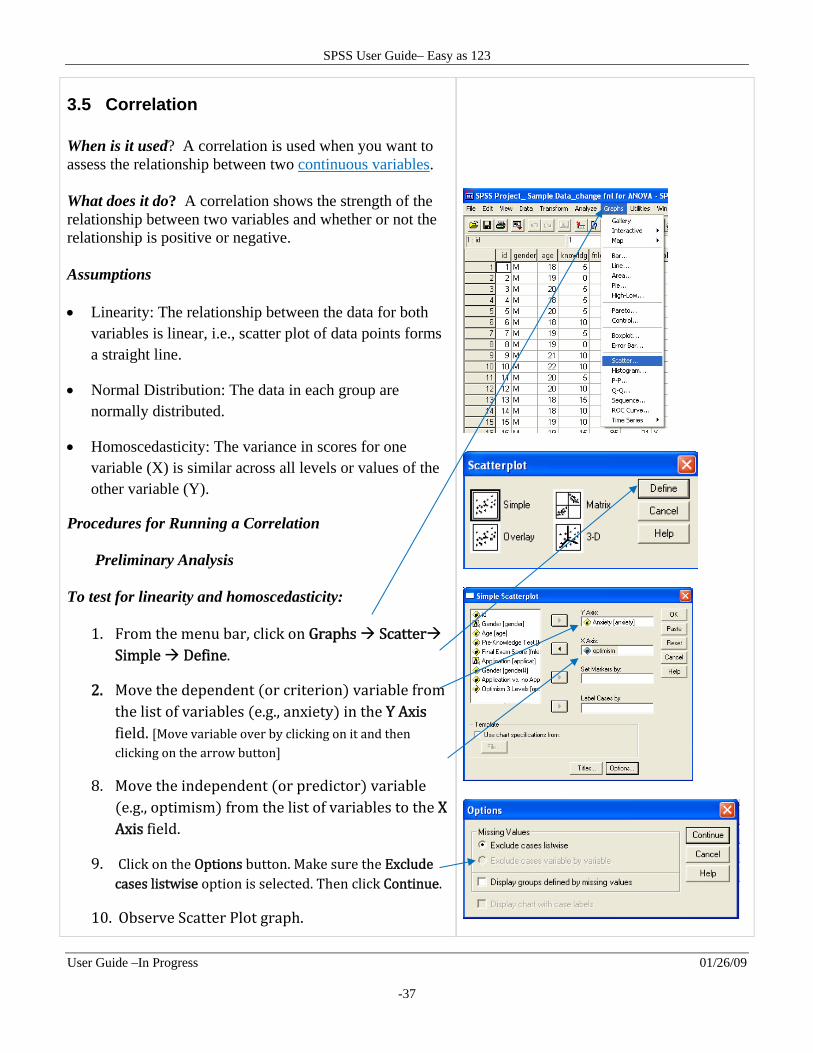
3.5 Correlation When is it used? A correlation is used when you want to assess the relationship between two continuous variables. What does it do? A correlation shows the strength of the relationship between two variables and whether or not the relationship is positive or negative. Assumptions Linearity: The relationship between the data for both

variables is linear, i.e., scatter plot of data points forms a straight line.

Normal Distribution: The data in each group are normally distributed.

Homoscedasticity: The variance in scores for one variable (X) is similar across all levels or values of the other variable (Y).

Procedures for Running a Correlation Preliminary Analysis To test for linearity and homoscedasticity:

1. From the menu bar, click on Graphs Scatter Simple Define.

2. Move the dependent or criterion variable from the list of variables e.g., anxiety in the Y Axis field. Move variable over by clicking on it and then clicking on the arrow button

8. Move the independent or predictor variable e.g., optimism from the list of variables to the X Axis field.

9. Click on the Options button. Make sure the Exclude cases listwise option is selected. Then click Continue.

10. Observe Scatter Plot graph.



-38

a. Check for Linearity

i. If a straight light can be drawn through the cluster of data point or the form of the scatter plot is similar to a straight line , there is linearity. Depicted in graph on right

ii. If the form of the data points in the scatter plot goes up and down i.e., curvilinear and a curved line would best fit the data points, the linearity assumption is violated.

b. Check for Homoscedasticity

i. If the cluster of data points is even from one end of line to the other, there is homoscedasticity. Depicted in the graph on right

ii. If the cluster of data points is not even and is narrow at one end and wide at the other, the assumption of homoscedasticity is violated.

To conduct Person product-moment correlation analysis:

1. From the menu bar, click on Analyze Correlate Bivariate.

2. Move the variables e.g., anxiety and optimism you want to correlate into the Variable field. Move variable over by clicking on it and then clicking on the arrow button

3. Make sure the “Pearson” method is selected for the correlation coefficient.

4. Keep “Two‐tailed” test of significance selected, if you are not certain about the direction of the relationship. If the direction of the relationship is hypothesized or predicted, select a one‐tailed



-39

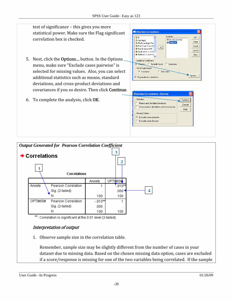
test of significance – this gives you more statistical power. Make sure the Flag significant correlation box is checked.

5. Next, click the Options… button. In the Options menu, make sure “Exclude cases pairwise” is selected for missing values. Also, you can select additional statistics such as means, standard deviations, and cross‐product deviations and covariances if you so desire. Then click Continue.

6. To complete the analysis, click OK.

Output Generated for Pearson Correlation Coefficient


1. Observe sample size in the correlation table.

Remember, sample size may be slightly different from the number of cases in your dataset due to missing data. Based on the chosen missing data option, cases are excluded if a score/response is missing for one of the two variables being correlated. If the sample

1

2

3

4



-40

size is not what you expected, check dataset for errors.

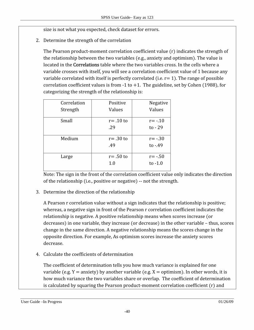
2. Determine the strength of the correlation

The Pearson product‐moment correlation coefficient value r indicates the strength of the relationship between the two variables e.g., anxiety and optimism . The value is located in the Correlations table where the two variables cross. In the cells where a variable crosses with itself, you will see a correlation coefficient value of 1 because any variable correlated with itself is perfectly correlated i.e. r 1 . The range of possible correlation coefficient values is from ‐1 to 1. The guideline, set by Cohen 1988 , for categorizing the strength of the relationship is:

Correlation Strength

Positive Values

Negative Values

Small r .10 to .29

r ‐.10 to ‐ 29

Medium r .30 to .49

r ‐.30 to ‐.49

Large r .50 to 1.0

r ‐.50 to ‐1.0

Note: The sign in the front of the correlation coefficient value only indicates the direction of the relationship i.e., positive or negative ‐‐ not the strength.

3. Determine the direction of the relationship

A Pearson r correlation value without a sign indicates that the relationship is positive; whereas, a negative sign in front of the Pearson r correlation coefficient indicates the relationship is negative. A positive relationship means when scores increase or decreases in one variable, they increase or decrease in the other variable – thus, scores change in the same direction. A negative relationship means the scores change in the opposite direction. For example, As optimism scores increase the anxiety scores decrease.

4. Calculate the coefficients of determination

The coefficient of determination tells you how much variance is explained for one variable e.g. Y anxiety by another variable e.g. X optimism . In other words, it is how much variance the two variables share or overlap. The coefficient of determinationis calculated by squaring the Pearson product‐moment correlation coefficient r and



-41

multiplying the product by 100. For example is the correlation is r ‐.81, the coefficient of determination is ‐.81 2 X 100 64.9 % or 65%. This indicates that optimism scores explain 65% of the variance in respondents’ anxiety scores.

5. Observe the level of significance

The level of significance is located directly under the correlation coefficient value in the Correlations table. If the value is less than .05, the correlation is statistically significant, whereas, if the value is greater than .05, the correlation is not statistically significant. Also, significant correlations are identified with asterisk s , and the notation at the bottom of the Correlation table indicates what the asterisk s means such as the level of significance and whether it was a one‐ or two‐tailed significance test. Please be aware that the significance level of a correlation can be influenced by the sample size – the larger the sample the more likely the correlation will be found significant. Thus, do not focus too much on the significance level – pay more attention to the size of the correlation.


A Pearson product‐moment correlation was conducted to evaluate the relationship between optimism measured by the General Optimism test GOT and perceived level of anxiety measured by the General Anxiety test GAT . Preliminary analyses showed that there were no violation of the assumptions of normality, linearity, and homoscedasticity. There was a strong, negative correlation between the two variables r ‐.81, N 100, p .01 indicating that high levels of optimism is associated with low levels of anxiety.



-42

4.0 Creating a Codebook A codebook includes information about what the data represent. The codebook should contain:

The full variable name for the abbreviated version of the variable name given in the spreadsheet with the data set.

o Example: “fnlexmgr”= final exam grade Coding for responses

o Labels for numerical responses. Example: Likert Scale Values 1, 2, 3, 4, 5 = Strongly Disagree, Somewhat Disagree,

Neutral, Somewhat Agree, Strongly Agree, respectively. o Numerical values for categorical or non-numeric responses.

Example: Male = 1 and Female = 2 Identification of reverse coded items.

o Reverse coded items are items on a survey that is written so that it represents the opposite of what is being measured. This is used to detect respondents who are not paying attention and are randomly answering questions. Example: You are measuring optimism. Item 1: “I usually think positively about what is going to happen in the future.” Item 10 “I usually think negatively about what is going to happen in the future.”

(reversed item) For item 1, on a Likert scale from 1-5 with 1 being Strongly Disagree and 5

being Strongly Agree, a higher score results in more optimism. For item 10, on a Likert scale from 1-5 with 1 being Strongly Disagree and 5

being Strongly Agree, a higher score results in less optimism. The item is reversed so the interpretation is reversed. To make the

interpretation of the items consistent, the reversed items have to be reversed coded such that 1=5, 2=4, 3=3, 4=2, 5=1. That way, higher scores represents more optimism.


User Guide – Draft Version 01/15/09

-A-1-

Glossary Bonferroni correction: Bonferroni correction is a method used to reduce Type 1 error rate (or Familywise error rate) when multiple significance tests are performed on the same data. The Bonferroni correction divides the significance level by the number of comparisons. If the significance level is set to .05 and there are six comparisons (or possible pairs of groups) in which a statistical test is conducted, the Bonferroni correction will divide the significance level (.05) by number of comparisons (6) resulting in a new significance level (.008); thus, resulting in a smaller significance level for each statistical test so that the chance of making a Type 1 error is reduced. If the correction is not applied the six comparisons would multiply the significance level by six resulting in a higher probability of Type 1 error (i.e., 6 x .05 = .300). Continuous Variable/Data A variable is continuous when the numeric data for that variable can take on infinite possible values or any value between two defined points. For example, if the variable is weight, the numeric data from the variable is continuous because it can take on any value (e.g., 55 lbs, 100.5 lbs, and 120.75 lbs.). [The total scores from responses on items using a Likert scale can be used as continuous data.] Contrasts: Contrasts are coefficients or coding used to designate which groups are being compared in an ANOVA with planned comparisons. The comparisons are pre-specified before the ANOVA is conducted by assigning contrasting coefficients to each group. The rule is that the coefficients assigned across the groups must equal zero. Thus, if you only want to compare two groups out of X amount of groups, you would assign a “1” to the first group of interest, a “-1” to the second group of interest, and a zero to the remaining groups. Here are examples of contrast coding.

Group 1 Group 2 Group 3 -1 0 1 -1 -1 2 2 -1 -1

In the first contrast (row 1), the coefficients are -1, 0, 1. This means that Group 1 is being compared to Group 3. The group(s) not included in the comparison can be assigned a zero as in this case. In the second contrast, the coefficients are -1, -1, 2. This indicates that Group 3 is being compared to Groups 1 and 2. In the third contrast, the coefficients are 2, -1, -1. This means that Group 1 is being compared to Groups 2 and 3. As mentioned earlier, the contrasting coefficients must add up to zero for each row (i.e., each contrast). Discrete Variable/Data A variable is discrete when the numeric data for that variable have a finite or limited number of possible values. All qualitative or categorical variables such as gender are discrete. For example gender or sex is a discrete variable. There is no natural sense of order for gender (i.e., male or female) and therefore is measured on nominal scale. Gender can be coded with any value such as Male = 1 and Female = 2 in order to appear numeric and allow quantitative analysis. However, the values or numbers used to represent gender type are meaningless. Some quantitative values are discrete such as a performance rated on a 1 – 4 scale.


User Guide – Draft Version 01/15/09

-A-2-

Interval measurement: The level of measurement is interval when the numerical values assigned have order and the distance between attributes is equal. For example interval between 50% and 60% score on a test is the same as the interval between 90% and 100% score on a test – there is a 10% difference. Test score would not be on the ratio level of measurement because there is no absolute zero (i.e., a 0% on a test does not necessarily mean a student has zero knowledge.) Levels of Measurement: The level of measurement describes the relationships among the values used to label attributes of a construct or variable. For example, if you have 5 numbers or values (1-5) that are used to represent responses to an item, the identified level of measurement will tell you whether the values are meaningful quantitatively, have order, have equal intervals, and/or have an absolute zero value. There are four levels of measurement: nominal, ordinal, interval and ratio. The level of measurement indicates which type of analyses can be used. Nominal measurement: For the nominal level of measurement, the numerical values only identify or name the attribute. The numbers assigned are not meaningful quantitatively. A categorical variable such as gender (with attributes: Male or Female) has a nominal level of measurement. Male can be labeled “1” and Female labeled “2” and vice versa. The numbers assigned have no meaning quantitatively – that is one is not higher than the other. Ordinal measurement: The level of measurement is ordinal when the numerical values assigned to the attributes indicate the rank-order of the attributes with the distance between the intervals being unknown. For example, if students were asked to indicate how often they visit the library: 1= daily, 2 = weekly, or 3 monthly; the types of responses or attributes is ordinal because we know that daily is more frequent then weekly and weekly if more frequent than monthly. However, the interval or time between the attributes is unknown. Ratio measurement: For the ratio of level of measurement, the numerical values assigned to the attributes have order, equal intervals, and an absolute zero that is meaningful. For example, the number of students attending class can be measured on a ratio level of measurement because zero number of students attending class actually means no presence of students. Type I error: A statistical probability of rejecting the null hypothesis (i.e., there is no difference between groups), when in fact the null is true. In other words the chances of concluding that there is a difference when in fact there is no difference. It is also known as a “false positive”.

THE BASICS OF DATA MANAGEMENT AND ANALYSIS A USER GUIDE … · 1.1 Purpose of the Basics of Data...

Documents

Transcript of THE BASICS OF DATA MANAGEMENT AND ANALYSIS A USER GUIDE … · 1.1 Purpose of the Basics of Data...