The Basel II IRB approach for credit portfolios: A survey · Figure 1 Credit Loss Distribution Loss...

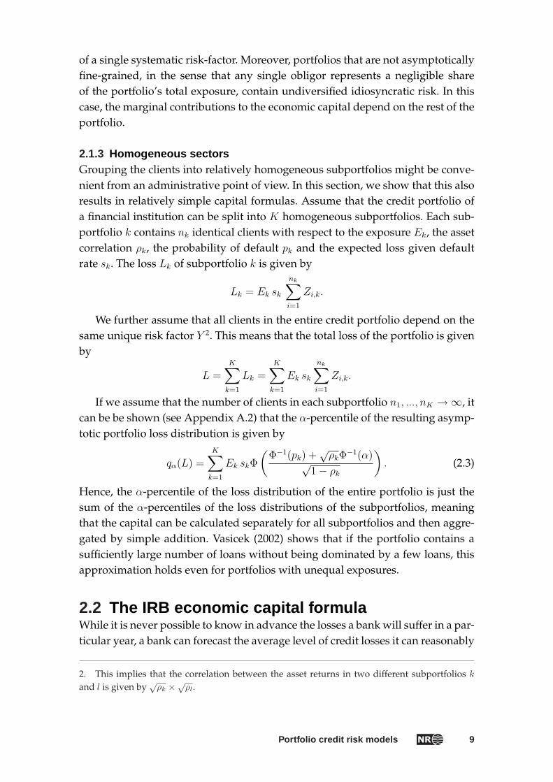
Figure 1Credit Loss Distribution

Loss

Pro

babi

lity

of L

oss

Note no SAMBA/33/05Author Kjersti Aas

Date October 2005

The Basel II IRBapproach for creditportfolios:A survey

Kjersti Aas

The authorAssistant research director Kjersti Aas

Norwegian Computing CenterNorsk Regnesentral (Norwegian Computing Center, NR) is a private, indepen-dent, non-profit foundation established in 1952. NR carries out contract researchand development projects in the areas of information and communication tech-nology and applied statistical modeling. The clients are a broad range of indus-trial, commercial and public service organizations in the national as well as theinternational market. Our scientific and technical capabilities are further devel-oped in co-operation with The Research Council of Norway and key customers.The results of our projects may take the form of reports, software, prototypes,and short courses. A proof of the confidence and appreciation our clients havefor us is given by the fact that most of our new contracts are signed with previouscustomers.

Title The Basel II IRB approach for creditportfolios:A survey

Author Kjersti Aas

Date October 2005

Publication number SAMBA/33/05

AbstractIn this report we review the Basel II IRB approach, including the theory used toderive its model foundation, and the interpretation of its parameters. The IRB ap-proach is a hybrid between a very simple statistical model of capital needs forcredit risk and a negotiated settlement. It is characterised by its computationalsimplicity; there is an analytical formula for the calculation of capital, and themodel is perfectly additive. However, this strength is also the cause of its weak-ness. The main assumptions have some negative consequences that are discussedin this report. Hence, the statistical model behind the Basel II IRB approach is notbest practice today, and certainly will not become so in the future. Even the BaselCommittee itself states that the IRB is work-in-progress, and will remain so longafter the implementation of Basel II (Basel Committee on Banking Supervision,2004b). We give some indications of how the IRB approach may be modified todeal with its weaknesses.

Keywords Basel II advanced IRB approach, credit portfolio risk,default probability, loss given default, assetcorrelations

Target group The Norwegian Finance Market Fund

Availability Closed

Project Finansmarked

Project number 220195

Research field Finance, insurance and power market

Number of pages 30

Copyright © 2005 Norwegian Computing Center

3

Contents

1 Introduction . . . . . . . . . . . . . . . . . . . . . . . . . 5

2 The advanced IRB approach . . . . . . . . . . . . . . . . . . 62.1 The Asymptotic Risk Factor approach. . . . . . . . . . . . 6

2.1.1 Default of one firm . . . . . . . . . . . . . . . . 62.1.2 Portfolio loss. . . . . . . . . . . . . . . . . . . 82.1.3 Homogeneous sectors . . . . . . . . . . . . . . 9

2.2 The IRB economic capital formula . . . . . . . . . . . . . 92.2.1 Maturity adjustments . . . . . . . . . . . . . . . 10

2.3 Parameters . . . . . . . . . . . . . . . . . . . . . . . 102.3.1 Probability of default . . . . . . . . . . . . . . . 112.3.2 Loss given default . . . . . . . . . . . . . . . . 112.3.3 Asset correlations . . . . . . . . . . . . . . . . 122.3.4 Exposure at default . . . . . . . . . . . . . . . . 13

3 The assumptions behind the IRB economic capital formula . . . 143.1 The two main assumptions . . . . . . . . . . . . . . . . 14

3.1.1 Assumption 1: Fine-grained portfolio . . . . . . . . 143.1.2 Assumption 2: Single systematic factor . . . . . . . 15

3.2 Other assumptions . . . . . . . . . . . . . . . . . . . . 163.2.1 Loss given default . . . . . . . . . . . . . . . . 163.2.2 Asset correlations . . . . . . . . . . . . . . . . 173.2.3 Asset distributions . . . . . . . . . . . . . . . . 17

4 Summary . . . . . . . . . . . . . . . . . . . . . . . . . . . 19

References . . . . . . . . . . . . . . . . . . . . . . . . . . . . 20

A Proofs of asymptotic capital rule . . . . . . . . . . . . . . . . 23A.1 Asymptotic loss for heterogeneous portfolio . . . . . . . . . 23A.2 Asymptotic loss for homogeneous portfolio . . . . . . . . . 25

B Portfolio variance and default correlation . . . . . . . . . . . . 28

C Asset correlations in the IRB approach . . . . . . . . . . . . . 29C.1 Corporate, sovereign, interbank . . . . . . . . . . . . . . 29C.2 Retail . . . . . . . . . . . . . . . . . . . . . . . . . . 29

Portfolio credit risk models 4

1 Introduction

In June 2004, the Basel Committee issued a revised framework on internationalconvergence of capital measurements and capital standards (Basel Committee onBanking Supervision, 2004b), which will serve as the basis for national rulemak-ing and implementation processes. The financial institutions may choose betweentwo approaches to calculate the capital requirement for credit risk; the standard-ised approach (essentially a slightly modified version of the current accord) andthe internal-ratings-based (IRB) approach. In the IRB approach, institutions areallowed to use their own measures for key drivers of credit risk as primary in-puts to the capital calculation. Hence, this approach is regarded as a first steptowards supervisory recognition of advanced credit risk models and economiccapital calculations.

In the IRB approach, regulatory minimum capital for a credit risk portfoliois calculated in a bottom-up approach, by determining capital requirements onthe asset level and adding them up. The capital requirements of assets are de-rived from risk weight formulas, which were developed considering a specialcredit portfolio model, the so-called Asymptotic Risk Factor (ASRF) model. Al-though there is no cited source or documentation behind this model, it is widelybelieved that the working paper version of Gordy (2003) was the precursor to theactual formulas. This model is characterised by its computational simplicity andthe property that the risk weights of single credit assets depend only on the char-acteristics of these assets, but not on the composition of the portfolio (portfolioinvariance).

In Chapter 2 we will give a description of the IRB approach, including thetheory used to derive the model, and the interpretation of its parameters. Themodel framework for the advanced IRB approach is based on two main assump-tions. These assumptions have some negative consequences that we will discussin Chapter 3. We will also indicate how the IRB approach may be modified todeal with them.


2 The advanced IRB approach

In the advanced IRB approach, regulatory capital requirements for unexpectedlosses are derived from risk weight formulas, which are based on the so-calledAsymptotic Risk Factor (ASRF) model. In this model, credit risk in a portfoliois divided into two categories, systematic and idiosyncratic risk. Systematic riskrepresents the effect of unexpected changes in macroeconomic and financial mar-ket conditions on the performance of borrowers. Idiosyncratic risk, on the otherhand, represents the effects of risk connected to individual firms. The idea behindthe ASRF model is that as the portfolio becomes more and more fine-grained, inthe sense that the largest individual exposures account for a smaller and smallershare of total portfolio exposure, idiosyncratic risk is diversified away on theportfolio level. The great advantage of the ASRF model is that the capital chargefor a lending exposure is based solely on loan-specific information. This allowsone to calculate capital charges on a decentralised loan-by-loan basis first, andthen aggregate these up to the portfolio-wide VaR afterwards. In Section 2.1 wereview this model. In Section 2.2 we give the actual formula used to computethe economic capital requirement in the advanced IRB framework, and finally inSection 2.3 we describe the interpretation of the parameters in this framework.

2.1 The Asymptotic Risk Factor approachThe ASRF approach assumes that the bank credit portfolio consists of a largenumber of relatively small exposures. If this is the case, idiosyncratic risk asso-ciated with individual exposures tends to be cancelled out, and only systematicrisks that affect many exposures have a material effect on portfolio losses. In theASRF approach, all systematic risk, like industry or regional risk, is modelledwith only one systematic risk factor. We first describe how default of a single firmis modelled in Section 2.1.1. Then, we outline how the single firm models can beused to derive a formula for the economic capital of the whole credit portfolio inSection 2.1.2. Finally, in Section 2.1.3 we give a slightly altered version of this for-mula, obtained when we group the clients into a set of relatively homogeneoussubportfolios.

2.1.1 Default of one firmThe ASRF approach is derived from an adaptation of the single asset model ofMerton (1974). In this approach, loans are modelled in a standard way as a claim


on the value of a firm. The value of the firm’s assets is measured by the priceat which the total of the firm’s liabilities can be purchased. Thus, the total valueof the firm’s assets is equal to the value of the stock plus the value of the debt.Loan default occurs if the market value of the firm’s assets falls below the amountdue to the loan. Thus the default distribution of a firm is a Bernoulli distribution,derived from the distribution of the value of the firm’s asset returns.

We start by assuming that the normalised asset return Ri of firm i in the creditportfolio is driven by a single common factor Y and an idiosyncratic noise com-ponent εi:

Ri =√

ρi Y +√

1− ρi εi, (2.1)

where Y and εi are i.i.d. N(0, 1), meaning that Ri is considered to have a stan-dardised Gaussian distribution. The component εi represents the risk specific toinstitution i and Y a common risk to all firms in the portfolio (representing thestate of the macro economy). It should be noted that the interpretation of the Ri’sas asset returns is merely intuitive, it is irrelevant to know the firms’ true assetreturns in this approach. It follows from Equation (2.1) that the assets of all firmsare multivariate Gaussian distributed and the assets of two firms i and j are cor-related with the linear correlation coefficient E[Ri, Rj] =

√ρi√

ρj1. Moreover, the

correlation between the asset return Ri and the common factor Y is√

ρi. Hence,√ρi is often interpreted as the sensitivity to systematic risk.

We define a binary random variable Zi for each firm, which takes on value1 (meaning that the ith obligor defaults) with probability pi and value 0 withprobability 1− pi. According to the theory of Merton (1974), we have

Zi,k = 1 if Ri,k ≤ Φ−1(pk) and Zi,k = 0 if Ri,k > Φ−1(pk),

where Φ(·) is the cumulative distribution function of the standard Gaussian dis-tribution.

The parameter pi is the unconditional default probability of obligor i. If theoutcome of the systematic risk factor was known, we could calculate the condi-tional probability of default by

P (Zi = 1|Y = y) = P (Ri ≤ Φ−1(pi)|Y = y)

= P (√

ρi Y +√

1− ρi εi ≤ Φ−1(pi)|Y = y)

= P (εi <Φ−1(pi)−√ρi Y√

1− ρi

|Y = y)

= Φ

(Φ−1(pi)−√ρi y√

1− ρi

).

1. It should be noted that asset return correlations and default correlations are not the same.Typically, the default correlation is much smaller than the asset correlation (Frey et al., 2001b), seeAppendix B for how they are related.


2.1.2 Portfolio lossVasicek (1977) showed that under certain conditions, Merton’s single asset

model can be extended to a model for the whole portfolio. The portfolio modelused in the advanced IRB approach (Gordy, 2003; Pykhtin and Dev, 2002) is verysimilar to Vasicek’s model. Inputs supplied by the bank include the exposure atdefault (EAD), the probability of default (PD), the loss given default (LGD) andthe effective remaining maturity (M). Given these inputs, the IRB capital chargeis computed by calculating capital charges on a decentralised loan-by-loan basis,and then aggregating these up to a portfolio-wide capital charge. In what follows,we describe the IRB approach in more detail.

Assume that we have a portfolio with N clients with different exposures Ei,asset correlations ρi, probabilities of default pi and loss given defaults si. Definethe exposure weight wi of client i by wi = Ei/

∑Ni=1 Ei, and let the portfolio loss

per dollar of exposure be given by

L =N∑

i=1

wi si Zi.

Provided that the clients depend on the same unique risk factor and no obligoraccounts for a significant fraction of the portfolio, it can be shown (see AppendixA.1) that as the number of clients in the portfolio N →∞, the α-percentile of theresulting portfolio loss distribution approaches the asymptotic value

qα(L) =N∑

i=1

wi siΦ

(Φ−1(pi) +

√ρiΦ

−1(α)√1− ρi

). (2.2)

Note that what is actually computed here is not the total capital charge, but thecapital charge per dollar of exposure.

Even though no bank can have an infinite number of loans, the asymptoticnature of the results does not diminish their practical usefulness. Gordy (2000)shows that the quantile is well-approximated by its asymptotic value for homo-geneous portfolios of reasonable size, and according to Schönbucher (2002a) theapproximation error becomes unacceptable only if very low asset return corre-lations (ρ < 1%), very few obligors (less than 500), or extremely heterogeneousexposure sizes (for instance one dominating obligor) are considered.

The remarkable property of Equation (2.2), apart from its simplicity is theasymptotic capital additivity; the total capital for a large portfolio of loans is theweighted sum of the marginal capitals for individual loans. In other words, thecapital required to add a loan to a large portfolio depends only on the propertiesof that loan/obligor and not on the portfolio it is added to. If this is the case, thecredit model is said to be portfolio invariant. Note that portfolio-invariance de-pends strongly on the asymptotic assumption, and especially on the assumption


of a single systematic risk-factor. Moreover, portfolios that are not asymptoticallyfine-grained, in the sense that any single obligor represents a negligible shareof the portfolio’s total exposure, contain undiversified idiosyncratic risk. In thiscase, the marginal contributions to the economic capital depend on the rest of theportfolio.

2.1.3 Homogeneous sectorsGrouping the clients into relatively homogeneous subportfolios might be conve-nient from an administrative point of view. In this section, we show that this alsoresults in relatively simple capital formulas. Assume that the credit portfolio ofa financial institution can be split into K homogeneous subportfolios. Each sub-portfolio k contains nk identical clients with respect to the exposure Ek, the assetcorrelation ρk, the probability of default pk and the expected loss given defaultrate sk. The loss Lk of subportfolio k is given by

Lk = Ek sk

nk∑i=1

Zi,k.

We further assume that all clients in the entire credit portfolio depend on thesame unique risk factor Y 2. This means that the total loss of the portfolio is givenby

L =K∑

k=1

Lk =K∑

k=1

Ek sk

nk∑i=1

Zi,k.

If we assume that the number of clients in each subportfolio n1, ..., nK →∞, itcan be be shown (see Appendix A.2) that the α-percentile of the resulting asymp-totic portfolio loss distribution is given by

qα(L) =K∑

k=1

Ek skΦ

(Φ−1(pk) +

√ρkΦ

−1(α)√1− ρk

). (2.3)

Hence, the α-percentile of the loss distribution of the entire portfolio is just thesum of the α-percentiles of the loss distributions of the subportfolios, meaningthat the capital can be calculated separately for all subportfolios and then aggre-gated by simple addition. Vasicek (2002) shows that if the portfolio contains asufficiently large number of loans without being dominated by a few loans, thisapproximation holds even for portfolios with unequal exposures.

2.2 The IRB economic capital formulaWhile it is never possible to know in advance the losses a bank will suffer in a par-ticular year, a bank can forecast the average level of credit losses it can reasonably

2. This implies that the correlation between the asset returns in two different subportfolios k

and l is given by√

ρk ×√ρl.


expect to experience. These losses are referred to as expected losses (EL). Lossesabove the expected levels are usually referred to as unexpected losses (UL). Insti-tutions know that these losses will occur now and then, but they cannot know inadvance the time of their arrival and their severity. Banks are in general expectedto cover their EL on an ongoing basis, e.g. by provisions and write-offs, because itrepresents just another cost component of the lending business. According to thisconcept, capital is only needed for covering unexpected losses. Hence, in Basel II,the banks are only required to hold capital against UL, meaning that the neededcapital per dollar of exposure is given by

Cα(L) = qα(L)− E(L) =N∑

i=1

wi si

[Φ

(Φ−1(pi) +

√ρiΦ

−1(α)√1− ρi

)− pi

], (2.4)

since the expected loss per dollar of exposure for the whole credit portfolio isgiven by

E(L) =N∑

i=1

wi si pi.

In Basel II, the confidence level α is set to 99.9%, i.e. an institution is expected tosuffer losses that exceed its economic capital once in a thousand years on average.

2.2.1 Maturity adjustmentsCredit portfolios consist of instruments with different maturities. Empirical evi-dence indicates that long-term credits are riskier than short-term credits. For in-stance, downgrades from one rating category to a lower one, are more likely forlong-term credits. Moreover, maturity effects are stronger for obligors with lowprobability of default. Consistent with these considerations, the Basel Commit-tee has proposed a maturity adjustment mi to be multiplied with each term ofthe economic capital computed from Equation (2.4). The maturity adjustment forclient i is given by (Basel Committee on Banking Supervision, 2004a)

mi =1 + (M − 2.5) b(pi)

1− 1.5 b(pi),

whereb(pi) = (0.11852− 0.05478× log(pi))

2,

and M is the maturity. In Basel II, M is set to 2.5 years for all rating grades. Thematurity adjustment is only done for the corporate borrower portfolio.

2.3 ParametersThe parameters to be determined for each client in the IRB approach are

· pi, the probability of default for client i.


· si, the loss given default for client i, which is the percentage of exposure thebank might loose in case client i defaults.

·√

ρi, the correlation between the asset return for client i and the commonfactor.

· Ei, the exposure at default for client i, which is an estimate of the amountoutstanding in case client i defaults.

The institutions may choose between two different versions of the IRB ap-proach; foundation IRB and advanced IRB. For any of the versions, the institu-tions are allowed to determine borrowers’ probabilities of default (PD) in theirown way. However, the institutions using the advanced IRB approach are alsopermitted to rely on their own estimates of loss given default (LGD) and ex-posure at default (EAD). In what follows, we describe the interpretation of theparameters in the Basel IRB framework.

2.3.1 Probability of defaultThe PDs are supposed to be obtained from the internal rating system of the bank.According to the Basel Accord, they should be average quantities, reflecting ex-pected default rates under normal business conditions.

Two kinds of models for determining probabilities of default are commonlyaddressed in the literature; accounting based models and market based models.Discriminant analysis and logistic regression models belong to the first class. Thepopular Z-score (Altman, 1968) is based on linear discriminant analysis, whileOhlsons O-Score (Ohlson, 1980) is based on generalised linear models (GLM)with the logit link function. Newer accounting based models are founded on neu-ral networks (Wilson and Sharda, 1994) and Generalised Additive Models (GAM)(Berg, 2004).

The market models are based on the value of a firm, set by the market. Onewell-known example is the Moody’s KMV model. Stock prices are commonlyused as proxies for the value of the firm. Hence, this kind of models require thatfirms are registered on a stock exchange, a circumstance which is not fulfilled formost small and medium sized borrowers.

2.3.2 Loss given defaultIn the capital formula in Equation (2.3) it is assumed that the loss given defaultrate (which is equal to one minus the recovery rate) is known and non-stochastic(Gordy, 2003). During an economic downturn, losses on defaulted loans are likelyto be higher than under normal business conditions, because for instance col-lateral values may decline. Average loss severity figures over long periods oftime can understate LGD rates during an economic downturn, and may therefore


need to be adjusted upward to appropriately reflect adverse economic conditions.Hence, one should choose conservative values in order not to underestimate therisk of the portfolio, and the Basel II capital formula requires that a “downturn”LGD is estimated for each client/risk segment. Due to the evolving nature ofbank practices in the area of loss given default quantification, the Basel Commit-tee has not proposed a specific rule for estimating the LGDs. Instead the banksare required to provide their own estimates.

Note that since one is supposed to use a “downturn” LGD, the EL in Equa-tion (2.4) is probably overestimated, since the “downturn” LGD will generallybe higher than the average one. Moreover, the capital requirement for defaultedassets will be 0. According to the Basel Committee, the latter is not desirable,since it does not cover systematic uncertainty in realised recovery rates for theseexposures. Hence, the committee has stated that an “average” LGD should beused for computing the EL for defaulted assets. For performing loans however,the “downturn” LGD should be used both to compute the loss percentile and theexpected loss.

2.3.3 Asset correlationsThe asset correlations needed as input in the ASRF model, determine in short,how the asset values of the borrowers depend on each other. It should be notedthat asset correlations and default correlations are not the same (see in AppendixB how they are related to each other). The input correlations also specify howthe asset values of the borrowers depend on the general state of the economy,represented by the systematic risk factor, Y .

In the IRB approach, the asset correlations are not to be estimated by thebanks. Instead they should be determined by formulas given by the Basel Com-mittee. These formulas are based on two empirical observations (Lopez, 2004);

· asset correlations decrease with increasing probability of default

· asset correlations increase with firm size.

This means that the higher the probability of default, the higher the idiosyncraticrisk components of an obligor. Moreover, conditional on a certain probability ofdefault, assets of small and medium sized enterprises are less correlated. Hence, iftwo companies of different size have the same PD, it follows that the larger one isassumed to have a higher exposure to the systematic risk factor. In other words,larger firms are more closely related to the general conditions in the economy,while smaller firms are more likely to default for idiosyncratic reasons. The BaselCommittee has provided different formulas for computing the asset correlationsfor different business segments. These are given in Appendix C.


2.3.4 Exposure at defaultUnder the advanced IRB approach, banks are allowed to use their own esti-mates of expected Exposure At Default (EAD) for each facility. Conceptually,EAD consists of two parts, the amount currently drawn, and an estimate of fu-ture draw downs of available, but untapped credit. Estimates of potential futuredraw downs (i.e. how the client may decide to draw unused commitments) areknown as credit conversion factors (CCFs). Since the CCF is the only random orunknown proportion of EAD, estimating EAD amounts to estimating this CCF.The CCF is generally believed to depend on both the type of loan and the type ofborrower. For example CCFs for credit cards are likely to be different from CCFsfor corporate credit. At present, literature on these issues as well as data sourcesare scarce, but some suggestions as to which characteristics of a credit shouldbe taken into account in EAD estimation is given Basel Committee on BankingSupervision (2005).


3 The assumptions behind the IRBeconomic capital formula

The IRB economic capital formula given in Equation (2.4) is characterised by itscomputational simplicity; there is an analytical formula for the calculation ofcapital, and the model is perfectly additive. However, these strengths are alsothe cause of its weaknesses. The main assumptions have some negative conse-quences. In this chapter we will discuss these consequences and indicate how theIRB approach may be modified to deal with them. First, Section 3.1 treats the twomost important underlying assumptions, and then Section 3.2 describes other re-quirements of the IRB approach.

3.1 The two main assumptionsThe development of the Basel II IRB approach was subject to some important re-strictions in order to fit supervisory needs. There should be an analytical formulafor the calculation of capital. Moreover, the model should be perfectly additive,or portfolio invariant, in the sense that the capital required for any given loanshould depend only on the risk of that loan and not on the portfolio it is addedto. These requirements impose strict assumptions on the diversification achievedwithin a bank portfolio:

· It must be assumed that the bank’s credit portfolio is infinitely fine-grained,in the sense that any single obligor represents a negligible share of the port-folio’s total exposure.

· It is assumed that a single, common systematic risk factor drives all de-pendence across credit losses in the portfolio, i.e. the bank must be well-diversified across all geographic and industrial sectors in a large economy.

Both of these assumptions are not always met by banks, especially by smallerinstitutions. If the first assumption is violated, IRB capital requirements may un-derstate the true capital requirements, while the second assumption could resultin a potential overestimation of portfolio risk.

3.1.1 Assumption 1: Fine-grained portfolioThe asymptotic capital formula given by Equation (2.4) is strictly valid only for aportfolio with infinitesimally small weights on its largest exposures. If a few large


companies constitute a relatively large part of the credit portfolio, there will bea residual of undiversified idiosyncratic (unsystematic) risk in the portfolio. Noreal-world portfolios are in fact fine-grained portfolio, and therefore, one mightquestion the relevance of the asymptotic formula. The asymptotic capital formulahave been derived under the assumption that all the idiosyncratic risk is com-pletely diversified away. Hence, it must underestimate the true capital, since anyfinite-size portfolio carries some undiversified idiosyncratic risk. Gordy (2003)shows that the remaining unsystematic risk is inversely proportional to the effec-tive number of loans. This form of credit concentration risk is sometimes knownas granularity, and may be addressed via granularity adjustment to the economiccapital. The Basel Committee recognised this initially and introduced a granu-larity adjustment in Basel Committee on Banking Supervision (2001). Since then,at least four different approaches to granularity adjustment have been proposedin the literature (Emmer and Tasche, 2005; Gordy, 2004; Martin and Wilde, 2002;Pykhtin and Dev, 2002).

As shown in Section 2.2, the economic capital formula doesn’t give extendedregulatory capital requirements for risk concentrations. However, according tothe Basel II Accord banks will have to demonstrate to the supervisors that theyhave established appropriate procedures to keep concentrations under control.Therefore, there is a need for quantitative tools with which to monitor risk con-centrations, as well as guidelines for capital buffers against such concentrations.In Sections 3.1.1 and 3.1.2, we have a closer look at the two assumptions.

3.1.2 Assumption 2: Single systematic factorThe problem associated with assuming a single systematic risk factor is perhapsmore difficult to address analytically than the granularity risk, but has greaterconsequences, especially for institutions with broad geographical and sectoraldiversification. A single-factor model cannot reflect segmentation effects, say byindustry branches. This failure to recognise the diversification effects of segmen-tation could result in an overestimation of portfolio risk. Diversification is oneof the key tools for managing credit risk, and it is of vital importance that thecredit portfolio framework used to calculate and allocate credit capital effectivelymodels portfolio diversification effects.

In reality, the global business cycle is composed of many small economic changes,which might be linked to geography (e.g. political shifts) or to prices of produc-tion inputs (e.g., oil). If different industries and geographic regions may experi-ence different cycles, they should be presented by distinct, though possibly corre-lated, systematic risk factors. Recently, several authors have proposed such multi-factor models, see e.g. Céspedes (2002); Céspedes et al. (2005); Chabaane et al.(2004); Hamerle et al. (2003); Pykhtin (2004); Schönbucher (2002a); Tasche (2005).


Moreover, commercial credit risk models like Creditrisk+ and the Portfolio Man-ager software of Moody’s KMV, typically use multiple factors for determiningportfolio risk. Hence, the theoretical justification for the single factor model isweak and does not correspond to best practice in banking.

3.2 Other assumptionsIn this section we describe other requirements on which the IRB approach isbased. First, the IRB approach assumes that the LGD rate is deterministic andindependent of the PD, while there is a reason to believe that the opposite isthe case. This issue will be treated in Section 3.2.1. Second, the asset correlationsare determined from the PDs, using a downward sloping relationship which hasbeen rejected by many recent studies. We will come back to this in Section 3.2.2.Finally, the IRB approach models the asset returns with a multivariate normaldistribution. However, many empirical investigations, see e.g. Frey et al. (2001a)reject the normal distribution because it is unable to model dependence betweenextreme events. In Section 3.2.3 we will have a closer look at this issue.

3.2.1 Loss given defaultThe IRB approach assumes that the LGDs are fixed deterministic quantities. Theargument for this is that the uncertainty of the LGD does not contribute signif-icantly to the risk of the client when compared with the PD volatility. In realityhowever, the LGD is not a fixed quantity and in the literature, it is quite commonto assume that the it is a random value between 0 and 1, see e.g. Altman et al.(2003); Frye (2000); Hu and Perraudin (2002); Pykhtin (2003). The beta distribu-tion is often considered appropriate for modelling the LGD, see e.g. Gupton andStein (2002), because it is bounded between two points and can assume a widerange of shapes.

Although the Basel II Accord emphasises the need to consider correlation ofPD and LGD, the capital formula in Equation (2.3) is linear in LGD and implicitlyassumes independence. This assumption is made to simplify the IRB approach,and has neither theoretical nor empirical support. Recently, several authors havestated that there is reason to believe that there is a dependence between defaultevents and losses given default. For example, a negative cyclical downturn islikely to produce an increase in the number of defaults, and at the same time adecrease in the number of recoveries. The dependence between default eventsand recovery rates may for instance be introduced through a factor that drivesboth default events and recovery rates (Frye, 2000; Pykhtin, 2003).


3.2.2 Asset correlationsAs can be seen from Equation (C.1), Basel II assumes a downward sloping re-lationship between the asset correlation and the probability of default, i.e. thecorrelation between the assets of low-risk firms is assumed to be higher than theones between high-risk firms. Several studies have produced results that contra-dict this relationship, see e.g. (Dietsch and Petey, 2004; Düllmann and Scheule,2003; Hamerle et al., 2003; Rösch, 2002). If in reality the two effects do not offseteach other, or worse if they reinforce each other, this could lead to a gross under-estimation of the size of extreme losses. While the negative relationship betweenthe asset correlation and the probability of default seems to be rejected by manyrecent studies, the decreasing relationship of the asset correlation with decreasingfirm size is generally supported, see e.g. Dietsch and Petey (2004); Düllmann andScheule (2003).

It should also be noted that the economic capital formula in Equation (2.4) isvery sensitive to the asset correlation parameters. In particular, if the asset corre-lations are a few percentage points higher than what Basel assumes for a high-riskclient (see Appendix B for how the asset correlation and probability of default arerelated to each other), the required capital may be significantly higher. Similarly,if it is lower that what Basel says for low-risk segments, their capital can be dras-tically reduced. Hence, the degree of dependence between firms, i.e. the size ofcorrelations in this model, very strongly influences portfolio risk, especially forhigh confidence levels α (Perli and Nayda, 2004; Wehrspohn, 2002).

An alternative to the formulas specified by the Basel Committee, is to estimatethe asset correlations from historical data. A direct estimation of these parame-ters, however, is not possible since the asset values are not observable. This prob-lem is sometimes bypassed by approximating asset returns by equity returns.However, this solution requires that firms are registered on a stock exchange, acircumstance which is not fulfilled for most small and medium sized borrowers.An alternative approach is to use observed data on default rates to estimate theasset correlations. Appendix C of Case (2003) presents a brief summary of empiri-cal methods to estimate asset correlations in practice, both from historical defaultrates and from historical economic-return-on-asset data.

3.2.3 Asset distributionsThe Basel credit risk portfolio model makes use of a multidimensional normaldistribution. Many empirical investigations, see e.g. Frey et al. (2001a), reject thenormal distribution because it is unable to model dependence between extremeevents. The assumption of a joint Gaussian distribution for the obligors’ asset re-turns has another weakness; it implies that it is very difficult to fit both the tailsand the main body of the portfolio credit loss distribution well (Schönbucher,


2002b). Hence, other multivariate distributions and copulas have been consid-ered, e.g. the multivariate Student’s t- and normal inverse Gaussian distribution(Wehrspohn, 2002), the Student’s t- and the grouped t-copula (Daul et al., 2003),other elliptical copulas (Frey et al., 2003; Schmidt, 2003) and Archimedean copu-las (Frey et al., 2003).


4 Summary

In this report we have reviewed the Basel II IRB approach, including the theoryused to derive its model, and the interpretation of its parameters. The IRB ap-proach is a hybrid between a very simple statistical model of capital needs forcredit risk and a negotiated settlement. It is characterised by its computationalsimplicity; there is an analytical formula for the calculation of capital, and themodel is perfectly additive. However, these strengths are, at the same time, thecause of its weaknesses. The main assumptions have some negative consequencesthat have been addressed in this report. Hence, the statistical model behind theBasel II IRB approach is not best practice today, and certainly will not becomeso in the future. Even the Basel Committee itself states that the IRB is work-in-progress, and will remain so long after the implementation of Basel II (Basel Com-mittee on Banking Supervision, 2004b). We have given some indications of howthe IRB approach may be modified to deal with its weaknesses.


References

E. I. Altman. Financial ratios, discriminant analysis and the prediction of corpo-rate bankruptcy. Journal of Finance, 23:589–609, 1968.

E. I. Altman, B. Brady, A. Resti, and A. Sironi. The link between default and re-covery rates: Theory, empirical evidence and implications. New York UniversityStern School of Business Department of Finance Working Paper Series, 2003.

Basel Committee on Banking Supervision. The new Basel Capital Accord. Con-sultative document, 2001.

Basel Committee on Banking Supervision. An Explanatory Note on the Basel IIIRB Risk Weight Functions. Consultative Document, 2004a.

Basel Committee on Banking Supervision. International Convergence of Capi-tal Measurement and Capital Standards. A Revised Framework. ConsultativeDocument, 2004b.

Basel Committee on Banking Supervision. Studies on the Validation of InternalRating Systems. Working Paper No. 14, May, 2005.

D. Berg. Bankruptcy prediction by generalized additive models. Submitted toEuropean Journal of Operational Research, 2004.

B. Case. Loss characteristics of commercial real estate loan portfolios, 2003. BaselII White Paper from Board of Governors of the Federal Reserve System (U.S.).

J. C. Garcia Céspedes. Credit Risk Modelling and Basel II. Algo Research Quar-terly, 5(1):57–66, 2002.

J. C. Garcia Céspedes, J. A. de Juan Herrero, A. Kreinin, and D. Rosen. A SimpleMulti-Factor "Factor Adjustment" for the Treatment of Diversification in CreditCapital Rules. Working paper, BBVA and Algorithmics Inc, 2005.

A. Chabaane, A. Chouillou, and J.-P. Laurent. Aggregation and credit risk mea-surement in retail banking. Banque & Marchés, 70:5–15, 2004.

S. Daul, E. De Giorgi, F. Lindskog, and A. McNeil. The grouped t-copula withan application to credit risk. RISK, 16:73–76, 2003.


M. Dietsch and J. Petey. Should SME exposures be treated as retail or corporateexposures? A comparative analysis of default probabilities and asset correlationsin French and German SMEs. Journal of Banking and Finance, 28:773–788, 2004.

K. Düllmann and H. Scheule. Determinants of the Asset Correlations of GermanCorporations and Implications for Regulatory Capital. University of Regens-burg Working Paper, 2003.

S. Emmer and D. Tasche. Calculating credit risk capital charges with the one-factor model. Journal of Risk, 7(2):85–101, 2005.

R. Frey, A. J. McNeil, and M. Nyfeler. Copulas and Credit Risk Models. RISK,pages 111–114, 2001a.

R. Frey, A. J. McNeil, and M. Nyfeler. Modelling Dependent Defaults: AssetCorrelations Are Not Enough! Working paper, University of Zurich, March,2001b.

R. Frey, A. J. McNeil, and M. Nyfeler. Dependent defaults in models of portfoliocredit risk. Journal of Risk, 6(1):59–92, 2003.

J. Frye. Depressing recoveries. RISK, 13:108–111, 2000.

M. Gordy. A comparative anatomy of credit risk models. Journal of Banking andFinance, 24:119–142, 2000.

M. Gordy. A risk-factor foundation for risk-based capital rules. Journal of Finan-cial Intermediation, 12:199–232, 2003.

M. Gordy. Granularity adjustment in portfolio credit risk measurement. InG. Szegö, editor, Risk Measures for the 21st Century. Wiley, 2004.

G. M. Gupton and R. M. Stein. LossCalc: Model for predicting Loss Given De-fault (LGD). Moody’s KMV, 2002.

A. Hamerle, T. Liebig, and D. Rösch. Credit Risk Factor Modeling and the BaselII IRB Approach. Discussion Paper Series 2: Banking and Financial Supervision, No02/2003, 2003.

Y. T. Hu and W. Perraudin. The dependence of recovery rates and defaults.Birbeck College Working paper, 2002.

A. Lopez. The empirical relationship between average asset correlation, firmprobability of default, and asset size. Journal of Financial Intermediation, 13(2):265–283, 2004.

R. Martin and T. Wilde. Unsystematic credit risk. RISK, 15(11), 2002.


R. C. Merton. On the pricing of corporate debt: The risk structure of interestrates. Journal of Finance, 29:449–470, 1974.

J. A. Ohlson. Financial ratios and the probabilistic prediction of bankruptcy.Journal of Accounting Research, 18:109–131, 1980.

R. Perli and W. I. Nayda. Economic and regulatory capital allocation for revolv-ing retail exposures. Journal of Banking and Finance, 28:789–809, 2004.

M. Pykhtin. Unexpected recovery risk. RISK, 16:74–78, 2003.

M. Pykhtin. Multi-factor adjustment. RISK, 17:85–90, 2004.

M. Pykhtin and A. Dev. Analytical approach to credit risk modelling. RISK, 15:26–32, 2002.

D. Rösch. Correlations and Business Cycles of Credit Risk: Evidence fromBankruptcies in Germany. University of Regensburg Working Paper, 2002.

R. Schmidt. Credit risk modelling and estimation via elliptical copulae. In CreditRisk: Measurement, Evaluation and Management, ed. G. Bohl, G. Nakhaeizadeh, S.T.Rachev, T. Ridder and K.H. Vollmer, Physica Verlag Heidelberg, pages 267–289, 2003.

P. J. Schönbucher. Factor Models for Portfolio Credit Risk. Working paper, Uni-versity of Bonn, 2002a.

P. J. Schönbucher. Taken to the limit: Simple and not-so-simple Loan Loss Dis-tributions. Working paper, University of Bonn, 2002b.

D. Tasche. Risk contributions in an asymptotic multi-factor framework. Workingpaper Technische Universität München, 2005.

O. Vasicek. An equilibrium characterization of the term structure. Journal ofFinancial Economics, 5:177–188, 1977.

O. A. Vasicek. The distribution of loan portfolio value. RISK, 15:160–162, 2002.

U. Wehrspohn. Credit Risk Evaluation: Modeling-Analysis-Management. PhDThesis, Faculty of Economics, University of Heidelberg, Germany, 2002.

R. Wilson and R. Sharda. Bankruptcy prediction using neural networks. DecisionSupport Systems, 11:545–557, 1994.


A Proofs of asymptotic capital rule

In Section 2.1, we presented two important results concerning the α-percentileof the asymptotic portfolio loss distribution. The first, given by Gordy (2003);Pykhtin and Dev (2002) and others, states that the asymptotic α-percentile ofthe loss per dollar exposure of a portfolio with N clients with different expo-sure weights wi, asset correlations ρi , probabilities of default pi and expected lossgiven default rates si, is given by

qα(L) =N∑

i=1

wi si Φ

(Φ−1(pi) +

√ρiΦ

−1(α)√1− ρi

)(A.1)

when N →∞, i.e. the number of clients in the portfolio becomes large, providedthe clients depend on the same unique risk factor and no obligor accounts for asignificant fraction of the portfolio. An outline of the proof of this result is givenin Appendix A.1.

The other, given by Schönbucher (2002a); Wehrspohn (2002) and others, statesthat the asymptotic α-percentile of the loss of a homogeneous portfolio with atotal exposure of E distributed on N identical clients with respect to asset cor-relations ρ, probabilities of default p, and expected loss given default rates s isgiven by

qα(L) = E s Φ

(Φ−1(p) +

√ρΦ−1(α)√

1− ρ

), (A.2)

when N →∞, provided the clients depend on the same unique risk factor and noobligor accounts for a significant fraction of the portfolio. The proof of this resultis given in Appendix A.2.

A.1 Asymptotic loss for heterogeneous portfolioIn this section, we outline the proof of the capital formula given in Equation (A.1).For the full proof, see Gordy (2003). Assume that we have a portfolio with N

clients with different exposures Ei, asset correlations ρi, probabilities of defaultpi and LGDs si. Assume further that they all depend on the same systematic riskfactor Y . Let the portfolio loss be given by

L =N∑

i=1

Ei si Zi,

where Zi = 1 if obligor i defaults. Further define Ui = si Zi and assume that theUis are bounded on the interval [−1, 1], and, conditionally on Y , are mutually


independent. Define the portfolio loss ratio LR as the ratio of the total losses tothe total portfolio exposure, i.e.,

LR =

∑Ni=1 Ei si Zi∑N

i=1 Ei

.

Assume now that the share of the largest exposure in the portfolio vanishes tozero as the number of exposures in the portfolio increases. It then might be shownthat

limn→∞

LR − E[LR|Y ] = 0, (A.3)

where the conditional expectation is given by

E[LR|Y ] =

∑Ni=1 Ei E[Ui|Y ]∑N

i=1 Ei

. (A.4)

Hence, in the limit, we need only know the distribution of E[LR|Y ] to answerquestions about the distribution of LR. The proof is given in Appendix A of Gordy(2003). It can also be shown that under the same assumptions

limn→∞

qα(LR)− qα (E[LR|Y ]) = 0. (A.5)

Strictly speaking, this result does not always hold, but it is approximately true forall practical purposes. The proof is given in Appendix B of Gordy (2003). Equation(A.5) allows substituting the quantiles of E[LR|Y ] (which may be relatively easilyto calculate) for the corresponding quantiles of the loss rato LR (which are hard tocalculate) as the portfolio becomes large. It should be emphasized that Equation(A.5) is obtained with minimal restrictions on the make-up of the portfolio. Theassets may have quite varied PD, LGD and exposure sizes. Moreover, there is norestriction on the relationship between Ei and the distribution of Ui. Hence if,for instance, high-quality loans tend also to be the largest loans, the result is stillvalid.

The final result is that

qα (E[LR|Y ]) = E[LR|qα(Y )]. (A.6)

To obtain this result, one must make some assumptions concerning the behaviourof E[LR|Y ], to make sure that there is no complex dependence between the tailquantiles of the loss distribution and the way the conditional expected loss foreach borrower varies with Y . The conditional expectation must for instance benon-decreasing in Y , see Gordy (2003) for the proof. The result in Equation (A.6)is important, because qα (E[LR|Y ]) in general may be quite complicated to com-pute, while Equation (A.4) states that E[LR|qα(Y )] is simply the exposure-weighedaverage of the individual assets’ conditional expected losses.


From Equations (A.4),(A.5) and (A.6) we have that

limn→∞

qα(LR) = qα (E[LR|Y ]) = E[LR|qα(Y )] =

∑Ni=1 Ei E [Ui|Y = Φ−1(α)]∑N

i=1 Ei

. (A.7)

Further, since the LGDs are assumed to be known and deterministic (see Section2.3.2)

E[Ui|Y = Φ−1(α)

]= si E

[Zi|Y = Φ−1(α)

]= si P

(Zi = 1|Y = Φ−1(α)

),

and from Section 2.1.1 we have

P(Zi = 1|Y = Φ−1(α)

)= si Φ

(Φ−1(pi)−√ρi Φ

−1(α)√1− ρi

).

Inserting the expression for E [Ui|Y = Φ−1(α)] into Equation (A.7) and the defini-tion of wi from Section 2.1.2, we get

limn→∞

qα(LR) =N∑

i=1

wi si Φ

(Φ−1(pi)−√ρi Φ

−1(α)√1− ρi

),

which is equal to the formula in Equation (A.1).

A.2 Asymptotic loss for homogeneous portfolioIn what follows, we assume that we have a homogeneous portfolio containing N

identical clients with respect to asset correlations ρ, probabilities of default p, andLGDs s. Moreover, the clients are assumed to depend on the same unique riskfactor. The aim of this section is give the proof the capital formula in Equation(A.2). The proof is taken from Schönbucher (2002a).

The portfolio loss for a certain year is

L = E s X,

i.e. the loss fraction X multiplied with the total exposure of the portfolio, E, andthe loss given default rate, s. Since the two latter are assumed to be deterministicquantities, it is sufficient to know the distribution of the loss fraction.

First, we are interested in determining the probability that exactly n out of theN clients will default. Define

p(y) = P (Zi = 1|Y = y) = Φ

(Φ−1(p)−√ρy√

1− ρ

), (A.8)

which is the probability of firm i defaulting, given that the systematic factor Y

takes the value y. Then conditional on Y = y, the probability of having n defaultsin the portfolio is binomially distributed:

P

(N∑

i=1

Zi = n|Y = y

)=

(N

n

)(p(y))n (1− p(y))N−n . (A.9)


Using the law of iterated expectations, the probability of n defaults is the expectedvalue of the conditional probability of n defaults, i.e.

P

(N∑

i=1

Zi = n

)= E

[P

(N∑

i=1

Zi = n|Y = y

)](A.10)

=

∫ ∞

−∞P

(N∑

i=1

Zi = n|Y = y

)φ(y) dy (A.11)

=

∫ ∞

−∞(p(y))n (1− p(y))N−n φ(y) dy. (A.12)

With the probability of n defaults given as shown above, the distribution of thenumber of defaults is

P

(N∑

i=1

Zi ≤ m

)=

m∑n=0

∫ ∞

−∞(p(y))n (1− p(y))N−n φ(y) dy. (A.13)

If N is very large, and the portfolio is infinitely granular (i.e. each exposureis set to be equal to 1/N , with large N , a simplification of the model is possi-ble (Schönbucher, 2002a). Conditional on a realisation y of the common factor Y ,obligor defaults are independent of each other. Therefore, in a very large portfo-lio, the law of large numbers ensures that the fraction of clients defaulting in theportfolio given Y = y is equal to the individual conditional default probability inEquation (A.8), i.e.

P

(1

N

N∑i=1

Zi = p(y)|Y = y

)= 1.

Hence, if we know Y , then we can predict the fraction of clients that will defaultwith certainty.

We want to determine the distribution function of the loss fraction X = 1N

∑Ni=1 Zi:

P (X ≤ x) = E [P (X ≤ x|Y = y)]

=

∫ ∞

−∞P (X ≤ x|Y = y) φ(y) dy

=

∫ ∞

−∞P (p(Y ) ≤ x|Y = y) φ(y) dy

=

∫ ∞

−∞I (p(y) ≤ x) φ(y) dy

=

∫ ∞

−y∗(x)

φ(y) dy

= Φ(y∗).

Here, y∗(x) must be chosen such that p(−y∗(x)) = x 1, i.e.

y∗(x) =

√1− ρΦ−1(x)− Φ−1(p)√

ρ.

1. We also have that p(y) from Equation (A.8) decreases in y, such that p(y) ≤ x for y > −y∗(x).


Hence,

P (X ≤ x) = Φ

(√1− ρΦ−1(x)− Φ−1(p)√

ρ

).

If the α-percentile of the loss fraction distribution is denoted xα, we have that

Φ

(√1− ρΦ−1(xα)− Φ−1(p)√

ρ

)= α,

meaning that

xα = Φ

(Φ−1(p) +

√ρΦ−1(α)√

1− ρ

).

Hence, the α-percentile of the loss distribution is obtained as

qα(L) = E s Φ

(Φ−1(p) +

√ρΦ−1(α)√

1− ρ

), (A.14)

which is equal to the formula in Equation (A.2).


B Portfolio variance and default cor-relation

In general, the portfolio variance is the sum of the variances and covariancesof the portfolio components. Assuming that the PDs, exposures, and LGDs areindependent, and that the two latter are non-stochastic, the portfolio variance isgiven by

σ2 =N∑

i=1

N∑j=1

κijσiσj

=N∑

i=1

N∑j=1

κij

√wi si pi (1− pi)

√wj sj pj (1− pj)

where N is the number of clients in the portfolio, and κij is the default correlationbetween client i and j. In the Basel II model, the default correlation κij can becomputed from the asset correlations ρi and ρj using

κij =Φ2

(Φ−1(pi), Φ

−1(pj),√

ρi√

ρj

)− pi pj√pi (1− pi) pj (1− pj)

. (B.1)

Here Φ2(·) is the bivariate normal cumulative distribution function.


C Asset correlations in the IRB ap-proach

The Basel Committee has provided different formulae for the asset correlationsfor different business segments. We give the formulae for bank, sovereign andcorporate borrowers in Section C.1, and for retail portfolios in Section C.2.

C.1 Corporate, sovereign, interbankThe asset correlation function used for bank and sovereign exposures is given by

ρi = 0.12× 1− e−50pi

1− e−50+ 0.24×

(1− 1− e−50pi

1− e−50

). (C.1)

According to the Basel Committee (Basel Committee on Banking Supervision,2004a), the proposed shape of the above exponentially decreasing functions arein line with the findings of empirical studies. For corporate borrowers, the corre-lations ρ are first computed by Equation (C.1) and then modified as follows

ρi − 0.04, Si ≤ 5 EUR

ρi − 0.04× (1− (Si − 5)/45), 5 EUR < S ≤ 50 EUR

ρ Si > 50 EUR.

Here, the Si is annual sales for firm i. Hence, for small firms the asset correlationsare lowered.

C.2 RetailThe Basel Committee has also provided specific mappings between probability ofdefault p and asset correlation ρ for the retail portfolios. The correlation formulae,which have an empirical basis (Basel Committee on Banking Supervision, 2004a),are as follows:

· Residental mortgagesρi = 0.15,

· Qualifying revolving retail exposures

ρi = 0.04,


· Other retail exposures

ρi = 0.03× 1− e−35p

1− e−35+ 0.16×

(1− 1− e−35p

1− e−35

).


The Basel II IRB approach for credit portfolios: A survey · Figure 1 Credit Loss Distribution Loss...

Documents

Transcript of The Basel II IRB approach for credit portfolios: A survey · Figure 1 Credit Loss Distribution Loss...